Unemployment in the Smets-Wouters Model:The GSW Model

Jordi Galí

April 2016

Jordi Galí () Unemployment in the Smets-Wouters Model: The GSW Model April 2016 1 / 11

Introduction

Medium-scale New Keynesian DSGE models (SW, CEE)

- good empirical fit- useful for forecasting and policy analysis- basis for in-house models at policy institutions

Shortcoming: no reference to unemployment

GSW: estimation of the "reformulated" Smets-Wouters model usingunemployment data

Issues:

- role of wage markup shocks in fluctuations- new measures of the output gap- sources of unemployment fluctuations

Jordi Galí () Unemployment in the Smets-Wouters Model: The GSW Model April 2016 2 / 11

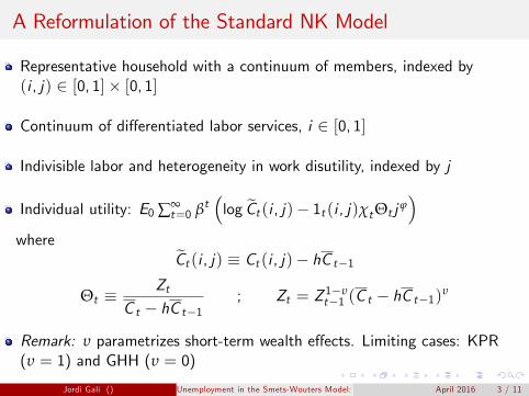
A Reformulation of the Standard NK Model

Representative household with a continuum of members, indexed by(i , j) ∈ [0, 1]× [0, 1]

Continuum of differentiated labor services, i ∈ [0, 1]

Indivisible labor and heterogeneity in work disutility, indexed by j

Individual utility: E0 ∑∞t=0 βt

(log C̃t (i , j)− 1t (i , j)χtΘt j ϕ

)where

C̃t (i , j) ≡ Ct (i , j)− hC t−1

Θt ≡Zt

C t − hC t−1; Zt = Z 1−υ

t−1 (C t − hC t−1)υ

Remark: υ parametrizes short-term wealth effects. Limiting cases: KPR(υ = 1) and GHH (υ = 0)

Jordi Galí () Unemployment in the Smets-Wouters Model: The GSW Model April 2016 3 / 11

A Reformulation of the Standard NK Model

Risk sharing withing the household: C̃t (i , j) = C̃t

Household utility:

E0∞

∑t=0

βtUt (Ct , {Nt (i)}) ≡ E0∞

∑t=0

βt(log C̃t − χtΘt

∫ 1

0

∫ Nt (i )

0j ϕdjdi

)= E0

∞

∑t=0

βt(log C̃t − χtΘt

∫ 1

0

Nt (i)1+ϕ

1+ ϕdi)

where Nt (i) : employment rate for type-i labor.

Jordi Galí () Unemployment in the Smets-Wouters Model: The GSW Model April 2016 4 / 11

A Reformulation of the Standard NK Model

Marginal rate of substitution for type-i labor:

−Un(i ),tUc ,t

= χtΘt C̃tNt (i)ϕ

= χtZtNt (i)ϕ

Average marginal rate of substitution (in logs)

mrst = zt + ϕnt + ξt

where ξt ≡ log χt .

Average wage markup

µw ,t ≡ (wt − pt )− (zt + ϕnt + ξt )

Jordi Galí () Unemployment in the Smets-Wouters Model: The GSW Model April 2016 5 / 11

Introducing Unemployment

Participation condition for individual (i , j):(1

C̃t

)(Wt (i)Pt

)≥ χtΘt j ϕ

Marginal participant in market for type-i labor, Lt (i):(1

C̃t

)(Wt (i)Pt

)= χtΘtLt (i)ϕ

Evaluating at a symmetric equilibrium (C̃tΘt = Zt), taking logs andintegrating over i ,

wt − pt = zt + ϕlt + ξt

where lt ≡∫ 10 lt (i) di is aggregate participation ("labor force").

Jordi Galí () Unemployment in the Smets-Wouters Model: The GSW Model April 2016 6 / 11

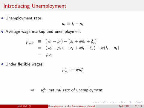
Introducing Unemployment

Unemployment rateut ≡ lt − nt

Average wage markup and unemployment

µw ,t ≡ (wt − pt )− (zt + ϕnt + ξt )

= (wt − pt )− (zt + ϕlt + ξt ) + ϕ(lt − nt )= ϕut

Under flexible wages:µnw ,t = ϕunt

⇒ unt : natural rate of unemployment

Jordi Galí () Unemployment in the Smets-Wouters Model: The GSW Model April 2016 7 / 11

The Identification Problem in Smets-Wouters

Calvo nominal wage setting (no indexation, standard preferences)

πwt = βEt{πwt+1} − λw (µw ,t − µnw ,t )

where µw ,t ≡ (wt − pt )− (ct + ϕnt + ξt )

The basic identification problem:

πwt = βEt{πwt+1} − λw [(wt − pt )− (ct + ϕnt )] + λw (ξt + µnw ,t )

Unemployment-based specification:

πwt = βEt{πwt+1} − λw ϕut + λwµnw ,t

Jordi Galí () Unemployment in the Smets-Wouters Model: The GSW Model April 2016 8 / 11

The Smets-Wouters Model: Remaining Ingredients

Capital accumulation, with investment adjustment costs

Calvo price and wage-setting, with partial indexation

Taylor-type interest rate rule

Multiple shocks:

- neutral and investment-specific technology- risk premium- government spending- monetary policy- price and wage markups- labor supply

Jordi Galí () Unemployment in the Smets-Wouters Model: The GSW Model April 2016 9 / 11

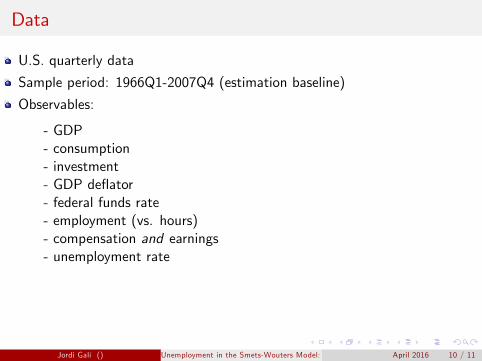
Data

U.S. quarterly data

Sample period: 1966Q1-2007Q4 (estimation baseline)

Observables:

- GDP- consumption- investment- GDP deflator- federal funds rate- employment (vs. hours)- compensation and earnings- unemployment rate

Jordi Galí () Unemployment in the Smets-Wouters Model: The GSW Model April 2016 10 / 11

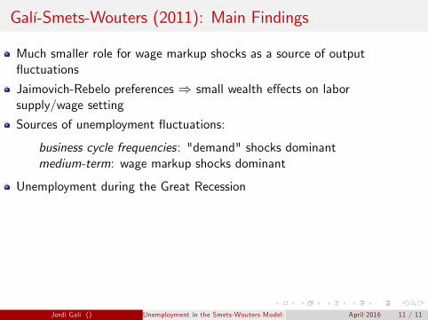
Galí-Smets-Wouters (2011): Main Findings

Much smaller role for wage markup shocks as a source of outputfluctuations

Jaimovich-Rebelo preferences ⇒ small wealth effects on laborsupply/wage setting

Sources of unemployment fluctuations:

business cycle frequencies: "demand" shocks dominantmedium-term: wage markup shocks dominant

Unemployment during the Great Recession

Jordi Galí () Unemployment in the Smets-Wouters Model: The GSW Model April 2016 11 / 11

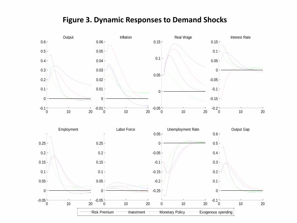
Figure 3. Dynamic Responses to Demand Shocks

0 10 20-0.1

0

0.1

0.2

0.3

0.4

0.5

0.6Output

Risk Premium Investment Monetary Policy Exogenous spending

0 10 20

-0.25

-0.2

-0.15

-0.1

-0.05

0

0.05Unemployment Rate

0 10 20-0.05

0

0.05

0.1

0.15

0.2

0.25

Employment

0 10 20-0.05

0

0.05

0.1

0.15

0.2

0.25

Labor Force

0 10 20-0.01

0

0.01

0.02

0.03

0.04

0.05

0.06Inflation

0 10 20-0.05

0

0.05

0.1

0.15Real Wage

0 10 20-0.1

0

0.1

0.2

0.3

0.4

0.5

0.6Output Gap

0 10 20-0.2

-0.15

-0.1

-0.05

0

0.05

0.1

0.15Interest Rate

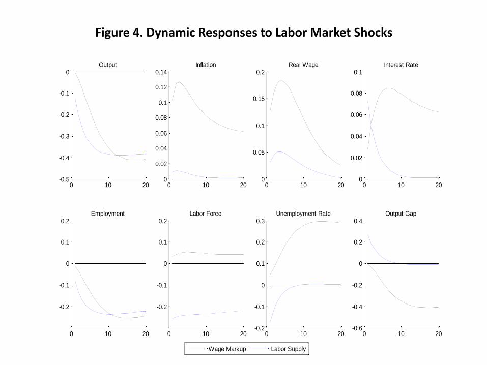
Figure 4. Dynamic Responses to Labor Market Shocks

0 10 20-0.5

-0.4

-0.3

-0.2

-0.1

0Output

Wage Markup Labor Supply

0 10 20-0.2

-0.1

0

0.1

0.2

0.3Unemployment Rate

0 10 20

-0.2

-0.1

0

0.1

0.2Employment

0 10 20

-0.2

-0.1

0

0.1

0.2Labor Force

0 10 200

0.02

0.04

0.06

0.08

0.1

0.12

0.14Inflation

0 10 200

0.05

0.1

0.15

0.2Real Wage

0 10 200

0.02

0.04

0.06

0.08

0.1Interest Rate

0 10 20-0.6

-0.4

-0.2

0

0.2

0.4Output Gap

0 10 200

0.2

0.4

0.6

0.8

1Output

Productivity Price Markup

0 10 20

-0.1

-0.05

0

0.05

0.1

0.15

Unemployment Rate

0 10 20-0.2

-0.15

-0.1

-0.05

0

0.05

0.1

Employment

0 10 20-0.2

-0.15

-0.1

-0.05

0

0.05

0.1

Labor Force

0 10 20-0.25

-0.2

-0.15

-0.1

-0.05

0

0.05

0.1Inflation

0 10 200

0.1

0.2

0.3

0.4Real Wage

0 10 20-0.5

-0.4

-0.3

-0.2

-0.1

0

0.1

0.2Output Gap

0 10 20-0.15

-0.1

-0.05

0

0.05Interest Rate

Figure 5. Dynamic Responses to Supply Shocks

0 5 10 15 20

-0.25

-0.2

-0.15

-0.1

-0.05

0

0.05

Unemployment Rate

0 5 10 15 20-0.1

-0.05

0

0.05

0.1

0.15

0.2

0.25

0.3Employment

0 5 10 15 20-0.2

-0.15

-0.1

-0.05

0

0.05

0.1

0.15

0.2Labor Force

Baseline model KPR-preferences

Figure 6. Monetary Policy Shocks and the Role of Wealth Effects

Figure 7. Two Measures of the Output Gap

1965 1970 1975 1980 1985 1990 1995 2000 2005 2010

-10

-8

-6

-4

-2

0

2

4

6

8

10

Outputgap with UR Outputgap without UR

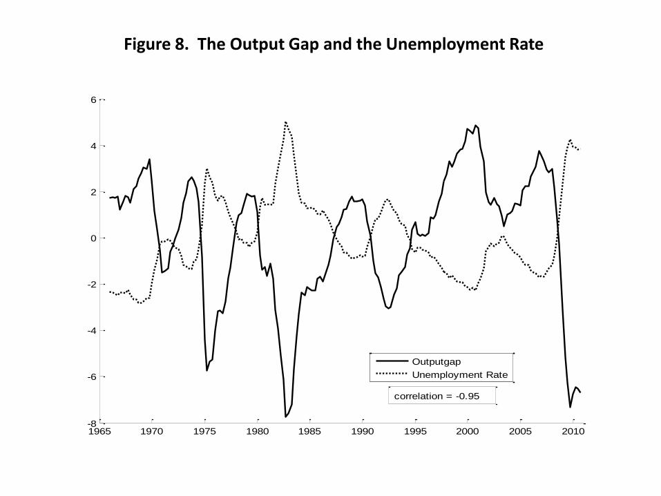
Figure 8. The Output Gap and the Unemployment Rate

1965 1970 1975 1980 1985 1990 1995 2000 2005 2010-8

-6

-4

-2

0

2

4

6

Outputgap

Unemployment Rate

correlation = -0.95

1965 1970 1975 1980 1985 1990 1995 2000 2005 2010-10

-8

-6

-4

-2

0

2

4

6

hp

bk

qt

cbo

model

Figure 9. The Output Gap vs. Detrended GDP

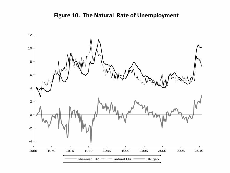
Figure 10. The Natural Rate of Unemployment

1965 1970 1975 1980 1985 1990 1995 2000 2005 2010

-4

-2

0

2

4

6

8

10

12

observed UR natural UR UR gap

Figure 11. Sources of Unemployment Rate Fluctuations

1965 1970 1975 1980 1985 1990 1995 2000 2005 20102

3

4

5

6

7

8

9

10

11Unemployment Rate decomposition

historical UR

supply shocks

demand shocks

1965 1970 1975 1980 1985 1990 1995 2000 2005 20102

3

4

5

6

7

8

9

10

11

historical UR

labor supply

wage mark-up

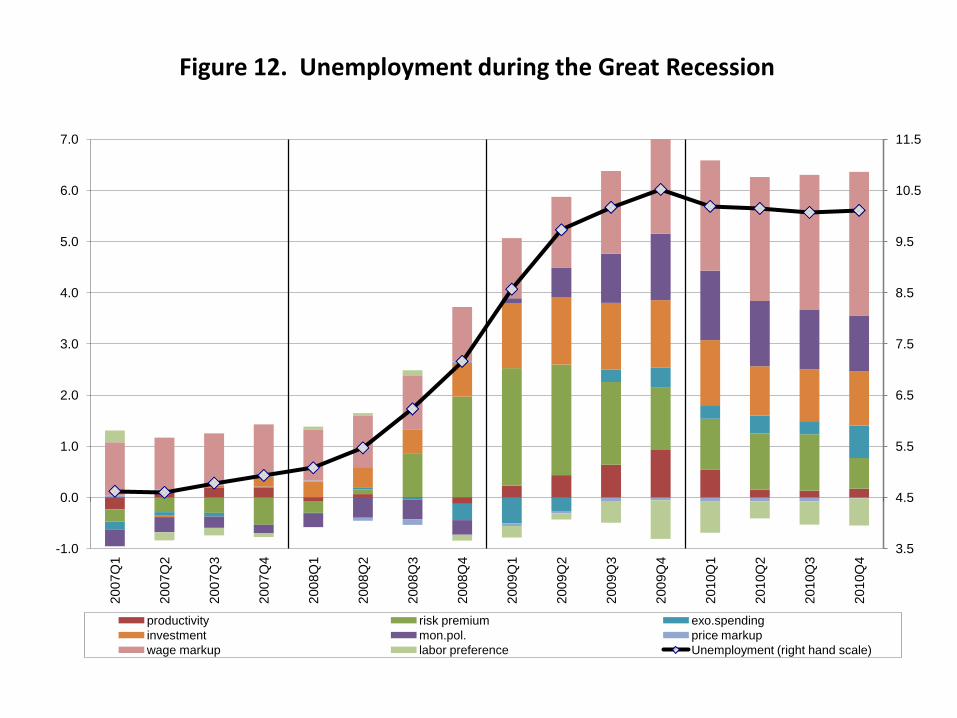
Figure 12. Unemployment during the Great Recession

3.5

4.5

5.5

6.5

7.5

8.5

9.5

10.5

11.5

-1.0

0.0

1.0

2.0

3.0

4.0

5.0

6.0

7.0

2007

Q1

2007

Q2

2007

Q3

2007

Q4

2008

Q1

2008

Q2

2008

Q3

2008

Q4

2009

Q1

2009

Q2

2009

Q3

2009

Q4

2010

Q1

2010

Q2

2010

Q3

2010

Q4

productivity risk premium exo.spendinginvestment mon.pol. price markupwage markup labor preference Unemployment (right hand scale)