Noname manuscript No.(will be inserted by the editor)

Hough Pyramid Matching: Speeded-up geometry re-ranking for largescale image retrieval

Yannis Avrithis and Giorgos ToliasNational Technical University of AthensIroon Polytexneiou 9 Zografou, Greece{iavr,gtolias}@image.ntua.gr

the date of receipt and acceptance should be inserted later

Abstract Exploiting local feature shape has made geom-etry indexing possible, but at a high cost of index space,while a sequential spatial verification and re-ranking stageis still indispensable for large scale image retrieval. In thiswork we investigate an accelerated approach for the latterproblem. We develop a simple spatial matching model in-spired by Hough voting in the transformation space, wherevotes arise from single feature correspondences. Using a his-togram pyramid, we effectively compute pair-wise affinitiesof correspondences without ever enumerating all pairs. OurHough pyramid matching algorithm is linear in the numberof correspondences and allows for multiple matching sur-faces or non-rigid objects under one-to-one mapping. Weachieve re-ranking one order of magnitude more images atthe same query time with superior performance comparedto state of the art methods, while requiring the same indexspace. We show that soft assignment is compatible with thismatching scheme, preserving one-to-one mapping and fur-ther increasing performance.

1 Introduction

Sub-linear indexing of appearance has been possible withthe introduction of discriminative local features and descrip-tor vocabularies [33]. Despite the success of the bag of wordsmodel, spatial matching is still needed to boost performance,especially at large scale. Geometry indexing is still in its in-fancy, either being limited to weak constraints [17], or hav-ing high index space requirements [2]. A second stage ofspatial verification and geometry re-ranking is the de factosolution of choice, where RANSAC approximations domi-nate. Re-ranking is linear in the number of images to match,hence its speed is crucial.

Address(es) of author(s) should be given

Exploiting local shape of features (e.g. local scale, ori-entation, or affine parameters) to extrapolate relative trans-formations, it is either possible to construct RANSAC hy-potheses by single correspondences [27], or to see corre-spondences as Hough votes in a transformation space [23].In the former case one still has to count inliers, so even withfine codebooks and almost one correspondence per feature,the process is quadratic in the number of (tentative) cor-respondences. In the latter, voting is linear in the numberof correspondences but further verification with inlier countappears unavoidable.

Flexible spatial models are more typical in recognition;these are either not invariant to geometric transformations,or use pairwise constraints to detect inliers without any rigidmotion model [21]. The latter are at least quadratic in thenumber of correspondences and their practical running timeis still prohibitive if our target for re-ranking is thousands ofmatches per second.

We develop a relaxed spatial matching model, which,similarly to popular pyramid match approaches [13], dis-tributes correspondences over a hierarchical partition of thetransformation space. Using local feature shape to generatevotes, it is invariant to similarity transformations, free ofinlier-count verification and linear in the number of corre-spondences. It imposes one-to-one mapping and is flexible,allowing non-rigid motion and multiple matching surfacesor objects. This model is compatible with soft assignment ofdescriptors to multiple visual words, preserving one-to-onemapping and further increasing performance.

Fig. 1 compares our Hough pyramid matching (HPM)to fast spatial matching (FSM) [27]. Both the foregroundobject and the background are matched by HPM, followingdifferent motion models; inliers from one surface are onlyfound by FSM. We show experimentally that flexible match-ing outperforms RANSAC-based approximations under anyfixed model in terms of precision. But our major achieve-

2 Y. Avrithis and G. Tolias

Fig. 1 Top: Inliers found by 4-dof FSM and affine-model LO-RANSAC for two images of Oxford dataset. Bottom: HPM matching,with all tentative correspondences shown. The ones in cyan have beenerased. The rest are colored according to strength, with red (yellow)being the strongest (weakest).

ment is speed: in a given query time, HPM can re-rank oneorder of magnitude more images than the state of the art ingeometry re-ranking. We give a more detailed account of ourcontribution in section 2 after discussing in some depth themost related prior work.

2 Related work

Given a number of correspondences between a pair of im-ages, RANSAC [12], along with various approximations,is still one of the most popular spatial verification meth-ods. It uses as evidence the count of inliers to a geomet-ric model (e.g. homography, affine, similarity). Hypothesesare generated on random sets of correspondences, depend-ing on model complexity. However, its performance is poorwhen the ratio of inliers is too low. Philbin et al. [27] gener-ate hypotheses from single correspondences exploiting localfeature shape. Matching then becomes deterministic by enu-

merating all hypotheses. Still, this process is quadratic in thenumber of correspondences.

Consistent groups of correspondences may first be foundin the transformation space using the generalized Houghtransform [3]. This is carried out by Lowe [23], but onlyas a prior step to verification. Tentative correspondences arefound via fast nearest neighbor search in the descriptor spaceand used to generate votes in the transformation space. Cor-respondences are single, exploiting local shape as in [27].Using a hash table, mapping to Hough bins is linear in thenumber of correspondences and performance depends on thenumber rather than the ratio of inliers. Still, multiple groupsneed to be verified for inliers and this may be quadratic inthe worst case.

Leibe et al. [20] propose a probabilistic extension of thegeneralized Hough transform for object detection. In theirvoting scheme, observed visual words vote for object hy-potheses based on their position relative to the object center.Votes in this case come from a number of training images,rather than a single matched image. Feature orientation isnot taken into account so the method is not rotation invari-ant, but the principle is the same.

Jegou et al. [17] use a weaker geometric model wherebygroups of correspondences only agree in their relative scaleand—independently—orientation. Feature correspondencesare found using a visual vocabulary. Scale and orientationof local features are quantized and stored in the inverted file.Hence, geometric constraints are integrated in the filteringstage of the search engine. However, because constraintsare weak, this model does not dispense with geometry re-ranking after all.

In an attempt to capture information on the neighbor-hood of local features, MSER regions are employed to groupfeatures into bundles in [37]. Consistency between orderingsof bundled features is used for geometric matching. How-ever, the reference frame of the MSER regions is not usedand features are projected on image axes instead, so rotationinvariance is lost. The same weakness applies to Zhou etal. [39], who binarize spatial relations between pairs of localfeatures. Similarly, Cao et al. [7] order features according tolinear and circular projections, but rely on a training phaseto learn the best spatial configurations.

Global feature geometry is integrated in the indexingprocess by Avrithis et al. [2]. A feature map is constructedfor each feature, encoding positions of all other features ina local reference frame, similarly to shape context [5]. Re-ranking is still used, though it is much faster in this case.The additional space requirements for each feature map arereduced by the use of hashing, but it is clear that this ap-proach does not scale well.

Closely related to our approach is the work of Zhanget al. [38], who set up a 2D Hough voting space based onrelative displacements of corresponding features. Fixed size

Hough Pyramid Matching 3

bins incur quantization loss, while the model supports trans-lation invariance only. Likewise, Shen et al. [32] apply sev-eral scale and rotation transformations to the query featuresand produce a 2D (translation) voting map for each databaseimage. Queries are costly, both in terms of time and spaceneeded for voting maps.

Whenever a single hypothesis may be generated by asingle correspondence, Hough-based approaches are prefer-able to RANSAC-based ones, because they are nearly in-dependent of the ratio of inliers and need to verify onlya subset of hypotheses. However, both share the use of afixed geometric model and need a parameter in verifying ahypothesis, e.g. bin size for Hough, or inlier threshold forRANSAC. Although there are attempts for parameter-freemethods [29], an entirely different approach is to use flexi-ble models, which is typical for recognition. In this case con-sensus is built among hypotheses only, operating on pairs ofcorrespondences.

For instance, multiple groups of consistent correspon-dences are identified with the flexible, semi-local model ofCarneiro and Jepson [8], employing pairwise relations be-tween correspondences and allowing non-rigid deformations.Similarly, Leordeanu and Hebert [21] build a sparse adja-cency (affinity) matrix of correspondences and greedily re-cover inliers based on its principal eigenvector. This spectralmodel can additionally incorporate different feature map-ping constraints like one-to-one.

One-to-one mapping is maybe reminiscent of early cor-respondence methods on non-discriminative features, but canbe very important when vocabularies are small, under thepresence of repeating structures, or e.g. with soft assignmentmodels [28]. Enqvist et al. [11] form a graph with corre-spondences as vertices and inconsistencies as edges. One-to-one mapping is easily incorporated by having multiplematches of a single feature form a clique on the graph. Incontrast, we form a graph with features as vertices and cor-respondences as edges. Multiple matches then form a con-nected component of the graph.

Other solutions include for instance the early spectralapproach by Scott and Longuet-Higgins [31], the quadraticprogramming approximation by Berg et al. [6], the contextdependent kernel by Sahbi et al. [30], and the linear pro-gramming formulation by Jiang and Yu [18]. Most flexiblemodels are iterative and at least quadratic in the number ofcorrespondences. They are invariant to geometric transfor-mations and resistant to ambiguous feature correspondencesbut not necessarily robust to outliers.

Relaxed matching processes like the one of Vedaldi andSoatto [36] offer an extremely attractive alternative in termsof complexity by employing distributions over hierarchicalpartitions instead of pairwise computations. The most pop-ular is by Grauman and Darell [13], who map features to ahistogram pyramid in the descriptor space, and then match

them in a bottom-up process. The benefit comes mainly fromapproximating similarities by bin size. Lazebnik et al. [19]apply the same idea to image space but in such a way thatgeometric invariance is lost. Attempts to handle partial sim-ilarity usually resort to optimization methods like [22].

It should be noted that although a pyramid is a way to in-crease robustness over flat histograms, it is still approximateas correspondences may be lost at quantization boundaries,even at coarse levels. The effect has been analyzed in [14],where it has been shown that empirical distortion is substan-tially lower than the theoretical upper bound.

3 Contribution

While the above relaxed methods apply to two sets of fea-tures, we rather apply the same idea to one set of corre-spondences (feature pairs) and aim at grouping accordingto proximity, or affinity. This problem resembles mode seek-ing [9][35], but our solution is a non-iterative, bottom-upgrouping process that is free of any scale parameter. We rep-resent correspondences in the transformation space exploit-ing local feature shape as in [23], but we form correspon-dences using a vocabulary as in [27][17] rather than nearestneighbors in descriptor space. Like pyramid match [13], weapproximate affinity by bin size, without actually enumerat-ing correspondence pairs.

We impose a one-to-one mapping constraint such thateach feature in one image is mapped to at most one fea-ture in the other. Indeed, this makes our problem similarto that of [21], in the sense that we greedily select a pair-wise compatible subset of correspondences that maximizea non-negative, symmetric affinity matrix. However we al-low multiple groups (clusters) of correspondences. Contraryto [11][21], our voting model is non-iterative and linear inthe number of correspondences.

To summarize our contribution, we derive a flexible spa-tial matching scheme whereby all tentative correspondencescontribute, appropriately weighted, to a similarity score be-tween two images. What is most remarkable is that no verifi-cation, model fitting or inlier count is needed as in [23], [27]or [8]. Besides significant performance gain, this yields adramatic speed-up. Our result is a very simple algorithmthat requires no learning and can be easily integrated intoany image retrieval process.

Our Hough pyramid matching has been introduced in [34].In this work, we extend our matching algorithm to accountfor soft assignment of visual words on the query side, pro-viding an alternative solution to enforce one-to-one map-ping. We further study the distribution of votes in the trans-formation space and derive a non-uniform space quantiza-tion scheme turning out to a considerable speed-up whileleaving performance almost unaffected. We give more de-

4 Y. Avrithis and G. Tolias

tails on the matching processing itself, more examples, anda number of additional experiments and comparisons.

4 Problem formulation

In a nutshell, we are looking for one or more transforma-tions that will make parts of one image align to parts of an-other. A number of transformation models is possible, butwe choose to develop our method for similarity, i.e. a fourparameter transformation consisting of translation, rotationand scale. Starting with our image representation, we for-malize our goal as an optimization problem below.

We assume an image is represented by a set P of localfeatures, and for each feature p ∈ P we are given its de-scriptor, position and local shape. We restrict discussion toscale and rotation covariant features, so that the local shapeand position of feature p are given by the 3× 3 matrix

F (p) =

[M(p) t(p)

0T 1

], (1)

where M(p) = σ(p)R(p) and σ(p), R(p), t(p) stand forisotropic scale, orientation and position, respectively. R(p)is an orthogonal 2×2 matrix with detR(p) = 1, representedby an angle θ(p). In effect, F (p) specifies a similarity trans-formation with respect to a normalized patch e.g. centeredat the origin with scale σ0 = 1 and orientation θ0 = 0.

Given two images P,Q, an assignment or correspon-dence c = (p, q) is a pair of features p ∈ P, q ∈ Q. Therelative transformation from p to q is again a similarity trans-formation given by

F (c) = F (q)F (p)−1 =

[M(c) t(c)

0T 1

], (2)

where M(c) = σ(c)R(c), t(c) = t(q) − M(c)t(p); andσ(c) = σ(q)/σ(p), R(c) = R(q)R(p)−1 are the relativescale and orientation respectively from p to q. This is a 4-dof transformation represented by a parameter vector

f(c) = (x(c), y(c), σ(c), θ(c)), (3)

where [x(c) y(c)]T = t(c) and θ(c) = θ(q) − θ(p). Henceassignments can be seen as points in a d-dimensional trans-formation spaceF ; d = 4 in our case, while affine-covariantfeatures would have d = 6.

An initial set C of candidate or tentative corresponden-ces is constructed according to proximity of features in thedescriptor space. There are different criteria, e.g. by nearestneighbor search given a suitable metric, or using a visualvocabulary (or codebook). Here we consider the simplestvocabulary approach where two features correspond whenassigned to the same visual word:

C = {(p, q) ∈ P ×Q : u(p) = u(q)}, (4)

where u(p) is the visual word (or codeword) of p. This is amany-to-many mapping; each feature in P may have multi-ple assignments to features in Q, and vice versa. Given as-signment c = (p, q), we define its visual word u(c) as thecommon visual word u(p) = u(q).

Each correspondence c = (p, q) ∈ C is given a weightw(c) measuring its relative importance; we typically use theinverse document frequency (idf) of its visual word. Givena pair of assignments c, c′ ∈ C, we assume an affinity scoreα(c, c′) measures their similarity as a non-increasing func-tion of their distance in the transformation space. Finally,we say that two assignments c = (p, q), c′ = (p′, q′) arecompatible if p 6= p′ and q 6= q′, and conflicting otherwise.For instance, c, c′ are conflicting if they are mapping twofeatures of P to the same feature of Q.

Our problem is then to identify a subset of pairwise com-patible assignments that maximizes the sum of the weighted,pairwise affinity over all assignment pairs. This subset ofC determines an one-to-one mapping between inlier fea-tures of P,Q, and the maximum value is the similarity scorebetween P,Q. It can be easily shown that this is a binaryquadratic programming problem [25] and we only target avery fast, approximate solution. In fact, we want to groupassignments according to their affinity without actually enu-merating pairs.

The spectral matching (SM) approach of [21] is an ap-proximate solution where the binary constraint is relaxedand optimization is reduced to eigenvector computation. Notethat being compatible does not exclude assignments fromhaving low affinity. This is a departure of our solution fromthat of [21], as it allows multiple groups of assignments,corresponding to high-density regions in the transformationspace. Spectral matching is a method we compare to in ourexperiments.

5 Hough Pyramid Matching

We assume that transformation parameters are normalizedor non-linearly mapped to [0, 1] (see section 7). Hence thetransformation space is F = [0, 1]d. While we formulatedour problem with d = 4, matching can apply to arbitrarytransformation spaces (motion models) of any dimension(degrees of freedom).

We construct a hierarchical partition

B = {B0, . . . , BL−1} (5)

of F into L levels. Each B` ∈ B is a partition of F into 2kd

bins (hypercubes), where k = L − 1 − `. The bins are ob-tained by uniformly quantizing each transformation param-eter, or partitioning each dimension into 2k equal intervalsof length 2−k. B0 is at the finest (bottom) level; BL−1 is atthe coarsest (top) level and has a single bin. Each partition

Hough Pyramid Matching 5

B` is a refinement of B`+1. Conversely, each bin of B` isthe union of 2d bins of B`−1.

Starting with the set C of tentative correspondences ofimages P,Q, we distribute correspondences into bins with ahistogram pyramid. Given a bin b, let

h(b) = {c ∈ C : f(c) ∈ b} (6)

be the set of correspondences with parameter vectors fallinginto b, and |h(b)| its count. We use this count to approxi-mate affinities over bins in the hierarchy, making greedy de-cisions upon conflicts to compute a similarity score of P,Q.This computation is linear-time in the number of tentativecorrespondences n = |C|.

5.1 Matching process

We recursively split correspondences into bins in a top-downfashion, and then group them again recursively in a bottom-up fashion. We expect to find most groups of consistent cor-respondences at the finest (bottom) levels, but we do go allthe way up the hierarchy to account for flexibility.

Large groups of correspondences formed at a fine levelare more likely to be true, or inliers. Conversely, isolatedcorrespondences or groups formed at a coarse level are ex-pected to be false, or outliers. It follows that each correspon-dence should contribute to the similarity score accordingto the size of the groups it participates in and the level atwhich these groups are formed. We use the count of a binto estimate a group size, and its level to estimate the pair-wise affinity of correspondences within the group: indeed,bin sizes (hence distances within a bin) are increasing withlevel, hence affinity is decreasing.

In order to impose a one-to-one mapping constraint, wedetect conflicting correspondences at each level and greedilychoose the best one to keep on our way up the hierarchy. Theremaining are marked as erased. Let X` denote the set of allerased correspondences up to level `. If b ∈ B` is a bin atlevel `, then the set of correspondences we have kept in b ish(b) = h(b) \X`. Clearly, a single correspondence in a bindoes not make a group, while each correspondence links tom − 1 other correspondences in a group of m for m > 1.Hence we define the group count of bin b as

g(b) = [|h(b)| − 1]+, (7)

where [x]+ = max{0, x}.Now, let b0 ⊆ . . . ⊆ b` be the sequence of bins contain-

ing a correspondence c at successive levels up to level ` suchthat bk ∈ Bk for k = 0, . . . , `. For each k, we approximatethe affinity α(c, c′) of c to any other correspondence c′ ∈ bkby a fixed quantity. This quantity is assumed a non-negative,

non-increasing level affinity function of k, say α(k). We fo-cus here on the decreasing exponential form

α(k) = 2−λk, (8)

where λ controls the relative importance between succes-sive levels, i.e. how relaxed the matching process is. Forλ = 1, affinity is inversely proportional to bin size, whichis in fact an upper bound on the actual distance between pa-rameter vectors. For λ > 1, lower levels of the pyramid be-come more significant and the matching process becomesless flexible.

Observe that there are g(bk) − g(bk−1) new correspon-dences joining c in a group at level k. Similarly to standardpyramid match [13], this gives rise to the following strengthof c up to level `:

s`(c) = g(b0) +∑k=1

α(k){g(bk)− g(bk−1)}. (9)

We are now in position to define the similarity scorebetween images P,Q. Indeed, the total strength of corre-spondence c is simply its strength at the top level, s(c) =

sL−1(c). Then, excluding all erased assignmentsX = XL−1and taking weights into account, we define the similarityscore by the weighted sum

s(C) =∑

c∈C\X

w(c)s(c). (10)

On the other hand, we are also in position to choose thebest correspondence in case of conflicts and impose one-to-one mapping. In particular, let c = (p, q), c′ = (p′, q′) betwo conflicting assignments. By definition (4), all four fea-tures p, p′, q, q′ share the same visual word, so c, c′ are ofequal weight: w(c) = w(c′). Now let b ∈ B` be the first(finest) bin in the hierarchy with c, c′ ∈ b. It then followsfrom (9) and (10) that their contribution to the similarityscore may only differ up to level `− 1. We therefore choosethe strongest one up to level ` − 1 according to (9). In caseof equal strength, or at level 0, we pick one at random.

5.2 Examples and discussion

A toy 2D example of the matching process is illustrated inFigures 2, 3, 4. We assume that assignments are conflictingwhen they share the same visual word, as denoted by color.As shown in Fig. 2, three groups of assignments are formedat level 0: {c1, c2, c3}, {c4, c5} and {c6, c9}. The first twoare then joined at level 1. Assignments c7, c8 are conflicting,and c7 is erased at random. Assignments c5, c6 are also con-flicting, but are only compared at level 2 where they sharethe same bin; according to (9), c5 is stronger because it par-ticipates in a group of 5. Hence group {c6, c9} is broken up,

6 Y. Avrithis and G. Tolias

c1

c2c3

c4c5

c6

c7

c8

c9

Level 0

c1

c2c3

c4c5

c6

c7

c8

c9

Level 1

c1

c2c3

c4c5

c6

c7

c8

c9

Level 2

Fig. 2 Matching of nine assignments on a 3-level pyramid in 2D space. Colors denote visual words, and edge strength denotes affinity. The dottedline between c6, c9 denotes a group that is formed at level 0 and then broken up at level 2, since c6 is erased.

p q similarity score

c1 (2 + 122 +

142)w(c1)

c2 (2 + 122 +

142)w(c2)

c3 (2 + 122 +

142)w(c3)

c4 (1 + 123 +

142)w(c4)

c5 (1 + 123 +

142)w(c5)

c6 0

c7 0

c8146w(c8)

c9146w(c9)

Fig. 3 Assignment labels, features and scores referring to Fig. 2. Herevertices and edges denote features (in images P,Q) and assignments,respectively. Assignments c5, c6 are conflicting, being of the form(p, q), (p, q′). Similarly for c7, c8. Assignments c1, . . . , c5 join groupsat level 0; c8, c9 at level 2; and c6, c7 are erased.

c6 is erased and finally c8, c9 join c1, . . . , c5 in a group of 7at level 2.

Apart from the feature/assignment configuration in im-ages P,Q, Fig. 3 also illustrates how the similarity scoreof (10) is formed from individual assignment strengths, wherewe have assumed that λ = 1, so that α(k) = 2−k. For in-stance, assignments c1, . . . , c5 have strength contributionsfrom all 3 levels, while c8, c9 only from level 2. Fig. 4 showshow these contributions are arranged in a (theoretical) n×naffinity matrix A. In fact, summing affinities over a row ofA and multiplying by the corresponding assignment weightyields the assignment strength, as illustrated in Fig. 3—notethough that the diagonal is excluded due to (7).

c1

c1

c2

c2

c3

c3

c4

c4

c5

c5

c8

c8

c9

c9

c6

c6

c7

c7

1

112

12

14

14

0

0

Fig. 4 Affinity matrix equivalent to the strengths of Fig. 3 accordingto (9). Assignments have been rearranged so that groups appear in con-tiguous blocks. Groups formed at levels 0, 1, 2 are assigned affinity1, 1

2, 14

respectively. Assignments are placed on the diagonal, which isexcluded from summation.

Finally, observe that the upper triangular part of A, re-sponsible for half the similarity score of (10), correspondsto the set of edges among assignments shown in Fig. 2, theedge strength being proportional to affinity. This reveals thepairwise nature of the approach [8][21], including the factthat one assignment cannot form a group alone.

Another example is that of Fig. 1, where we match tworeal images of the same scene from different viewpoints. Alltentative correspondences are shown, but colored accord-ing to the strength they have acquired through the matchingprocess. There are a few mistakes, which is expected sinceHPM is really a fast approximation. However, it is clear thatthe strongest correspondences, contributing most to the sim-ilarity score, are true inliers. There may be no non-rigid mo-

Hough Pyramid Matching 7

−1.5 −1 −0.5 0 0.5 1 1.5−1.5

−1

−0.5

0

0.5

1

1.5

horizontal translation, x

vert

ical

tran

slat

ion,y

assignmenterased

−1 −0.5 0 0.5 10

π/4

π/2

3π/4

π

5π/4

3π/2

7π/4

2π

log-scale, log σ

orie

ntat

ion,θ

assignmenterased

Fig. 5 Correspondences of the example in Fig. 1 as votes in 4Dtransformation space. Two 2D projections are depicted, separately fortranslation (x, y) (above) and log-scale / orientation (log σ, θ) (below).Translation is normalized by maximum image dimension. Orientationis shifted by 5π/16 (see section 7). There are L = 5 levels and we arezooming into the central 8 × 8 (16 × 16) bins above (below). Edgesrepresent links between assignments that are grouped in levels 0, 1, 2only. Level affinity α is represented by three tones of gray with blackcorresponding to α(0) = 1.

tion or relative motion of different objects like two cars, yetthe 3D scene geometry is such that not even a homographycan capture the motion of all visible surfaces. Indeed, theinliers to an affine model with RANSAC are only a smallpercentage of the ones shown here.

In analogy to the toy example of Fig. 2, Fig. 5 illustratesmatching of assignments in the Hough space. Observe howassignments get stronger and contribute more by groupingaccording to proximity, which is a form of consensus. HPMtakes no more than 0.6ms to match this particular pair ofimages, given the features, visual words, and tentative cor-respondences.

5.3 The algorithm

The matching process is outlined more formally in algo-rithm 1. It follows a recursive implementation: code beforethe recursive call of line 12 is associated to the top-downsplitting process, while after that to bottom-up grouping.For brevity, variables or functions that are used in someblock of code without definition or initialization are consid-ered global. For instance weights w(c) are global to HPM,strengths s(c) are global to HPM-REC and ERASE, and so one.g. for B, L, X . On the other hand, C is redefined locally.In fact, |C| is decreasing as we go down the hierarchy.

Algorithm 1 Hough Pyramid Matching1: procedure HPM(assignments C, levels L)2: X ← ∅; B ← PARTITION(L) . erased; partition3: for all c ∈ C do s(c)← 0 . strengths4: HPM-REC(C,L− 1) . recurse at top5: return score

∑c∈C\X w(c)s(c) . see (10)

6: end procedure7:8: procedure HPM-REC(assignments C, level `)9: if |C| < 2 ∨ ` < 0 return

10: for all b ∈ B` do h(b)← ∅ . histogram11: for all c ∈ C do h(β`(c))← h(β`(c)) ∪ c . quantize12: for all b ∈ B` do HPM-REC(h(b), `− 1) . recurse down13: for all b ∈ B` do14: X ← X∪ ERASE(h(b))15: h(b)← h(b) \X . exclude erased16: if |h(b)| < 2 continue . exclude isolated17: if ` = L− 1 then a← 1 else a← 1− 2−λ

18: for all c ∈ h(b) do s(c)← s(c) + a2−λ`g(b) . (9)19: end for20: end procedure

Assignment of correspondences to bins is linear-time in|C| in line 11, though equivalent to (6). B` partitions F foreach level `, so given a correspondence c there is a uniquebin b ∈ B` such that f(c) ∈ b. We then define a constant-time mapping β` : c 7→ b by uniformly quantizing parametervector f(c) at level `. Storage in bins is sparse and linear-space in |C|; complete partitions B` are never really con-structed.

Computation of strengths in lines 17-18 of algorithm 1 isequivalent to (9). In particular, substituting (8) into (9) andmanipulating similarly to [13] yields

s(c) = g(b0) +

L−1∑k=1

2−λk(g(bk)− g(bk−1)) (11)

= a

L−2∑k=0

2−λkg(bk) + 2−λ(L−1)g(bL−1), (12)

where a = 1− 2−λ.Given a set of assignments in a bin, optimal detection of

conflicts can be a hard problem. In function ERASE of al-gorithm 2, we follow a very simple approximation whereby

8 Y. Avrithis and G. Tolias

(u1, u2)

(u2, u3)

(u1)

(u2)

(u3)

(a)

(u1, u2)

(u2, u3)

(u1)

(u2)

(u3)

(b)

Fig. 6 Detection of conflicts based on (a) visual word classes and(b) component classes, under soft assignment. Vertices on the left(right) represent query (database) features. Labels denote assigned vi-sual words, which are multiple for the query features. Same color de-notes assignments in conflict.

two assignments are conflicting when they share the samevisual word. This avoids storing features; and makes sensebecause with a fine vocabulary, features are uniquely mappedto visual words, e.g. 92% in our test sets—see section 8 fordetails.

Algorithm 2 Erase using visual word classes1: procedure ERASE(assignments C)2: x← ∅; U ← ∅;3: for all c ∈ C do U ← U ∪ u(c) . common visual words4: for all u ∈ U do e(u)← ∅ . visual word classes5: for all c ∈ C do e(u(c))← e(u(c)) ∪ c6: for all u ∈ U do x← x ∪ e(u) \ argmaxc∈e(u) s(c)7: return erased assignments x . all but strongest8: end procedure

For all assignments h(b) of bin b we first construct theset U of common visual words. This is done in line 3, whereu(c) is the visual word assigned to c. Then, in lines 4-5, wedefine for each visual word u ∈ U the visual word classe(u), that is, the set of all assignments mapped to u. Ac-cording to our assumption, all assignments in a class are(pairwise) conflicting. Therefore, we keep the strongest as-signment in each class, erase the rest and update X .

It is clear that all operations in each recursive call on binb are linear in |h(b)|. SinceB` partitions F for all `, the totaloperations per level are linear in n = |C|. Hence the timecomplexity of HPM is O(nL).

Algorithm 3 Erase using connected component classes1: procedure ERASE-CC(connected components Z)2: x← ∅;3: for all z ∈ Z do e(z)← E(z) . component classes4: for all z ∈ Z do x← x ∪ e(z) \ argmaxc∈e(z) s(c)5: return erased assignments x . all but strongest6: end procedure

6 Matching under soft assignment

The use of a vocabulary always incurs quantization loss. Acommon strategy for partially recovering from this loss isto assign descriptors to multiple visual words, in practice asmall number of nearest neighbors in the vocabulary [28].This soft assignment is preferably applied on the query im-age only, since inverted file memory requirements are leftunaffected [17]. We explore here the use of soft assignmentwith HPM, following the latter choice both in the filteringand re-ranking phase.

In the case of hard assignment, the detection of conflict-ing assignments has been based on the observation that ahigh percentage of features are uniquely mapped to visualwords. Unfortunately, this is not the case with soft assign-ment: the percentage of uniquely mapped features drops sig-nificantly, e.g. 85% (80%) for 3 (5) nearest neighbors in ourtest sets—see section 8 for details.

Figure 6(a) illustrates the detection of conflicts using vi-sual word classes under soft assignment. The database im-age has three features in this example, assigned to three dif-ferent visual words u1, u2, u3 respectively, while the queryimage has two features soft-assigned to u1, u2 and u2, u3 re-spectively. There are three visual word classes in this case,and keeping one assignment from each class according to al-gorithm 2 leads to a one-to-many mapping, with one of thequery features mapping to two database features.

We therefore introduce an alternative solution which canalways preserve one-to-one mapping, without significant in-crease in complexity. Given two images P,Q, the union offeatures V = P ∪ Q and the set of assignments C can beseen as an undirected graph G = (V,C), where each fea-ture is a vertex and each assignment is an edge. In fact, thegraph is bipartite, as each edge always joins a vertex of P toa vertex of Q.

Under this representation, we compute the set Z of con-nected components (maximally connected subgraphs) of G.In practice, using the union find algorithm with a disjoint-set data structure, this task is quasi-linear in the number ofedges (assignments), hence in the number of vertices (fea-tures). The assignments of each component are used to de-fine a component class. Component classes replace the vi-sual word classes of algorithm 2. In particular, all assign-ments in the same component are considered pairwise con-flicting, and only one is kept. Observe that isolated verticesare features participating in no assignments, implying thattheir components have no edges and are ignored.

Figure 6(b) illustrates conflicts using this scheme for theexample of 6(a). There is only one connected component inthis case, only one assignment is kept, and one-to-one map-ping is preserved. This holds in general: all assignments ofone feature always belong to the same component, so keep-ing one assignment from each component yields at most one

Hough Pyramid Matching 9

Fig. 7 Examples of HPM matching. (Top) hard assignment, visual word classes. (Middle) Soft assignment with 3 nearest neighbors, componentclasses. (Bottom) direct descriptor matching with ratio test [23], component classes. The color scheme is the same as in Fig. 1.

assignment per feature. Of course, the scheme of Fig. 6(b) ismore strict than necessary; for instance, it misses one secondassignment that may be valid. On the other hand, this is ben-eficial in reducing additional votes of background featuresdue to soft assignment.

The modified function ERASE-CC is summarized in Al-gorithm 3, where visual word classes e(u) are replaced bycomponent classes e(z) and E(z) in line 3 stands for theset of edges of z (which is a graph itself). Both kinds ofclasses are treated as equivalence classes with one represen-

tative only selected from each. As in the example of 6, thisscheme can be too strict, especially when the vocabulary isnot fine enough. On the other hand, it is applicable even inthe absence of a vocabulary, for instance when feature cor-respondences are determined by direct computations in thedescriptor space.

Matching of two real images under different assignmentand ERASE schemes is shown in Fig. 7. It is clear that HPMcan work perfectly well when descriptors are not quantizedand visual words are not available. In fact, this yields the

10 Y. Avrithis and G. Tolias

best matching quality. Hence HPM is not limited to im-age retrieval and can be applied to different matching sce-naria, although finding correspondences from descriptors ismuch more expensive than matching itself. The use of a vo-cabulary with soft assignment yields fewer ‘inliers’ (assign-ments with significant strength contribution); hard assign-ment yields even less.

7 Implementation

7.1 Indexing and re-ranking

HPM turns out to be so fast in practice that we integrateit into a large scale image retrieval engine to perform geo-metric verification and re-ranking. We construct an invertedfile structure indexed by visual word and for each featurein the database we store quantized location, scale, orienta-tion and image id. Given a query, this information is suffi-cient to perform the initial, sub-linear filtering stage eitherby bag of words (BoW) [33] or weak geometric consistency(WGC) [17].

A number of top-ranking images are marked for re-rank-ing. For each query feature, we retrieve tentative assign-ments from the inverted file once more, but now only formarked images. For each assignment c found, we computethe parameter vector f(c) of the relative transformation andstore it in a collection indexed by marked image id. Given allassignments and parameter vectors, we match each markedimage to the query using HPM. Finally, we normalize scoresby marked image BoW `2 norm and re-rank.

7.2 Quantization

We treat each relative transformation parameter x, y, σ, θof (3) separately. Translation t(c) in (2) refers to the coor-dinate frame of the query image, Q. If r is the maximumdimension of Q in pixels, we only keep assignments withhorizontal and vertical translation x, y ∈ [−3r, 3r]. We alsofilter assignments such that σ ∈ [1/σm, σm], where σm =

10 is above the range of any feature detector, so anythingabove that may be considered noise. We compute logarith-mic scale, normalize all ranges to [0, 1] and quantize param-eters uniformly.

We also quantize local feature parameters of the databaseimages: with L = 5 levels, each parameter is quantized into16 bins. Our space requirements per feature, as summarizedin Table 1, are then exactly the same as in [17]. On the otherhand, query feature parameters are not quantized. It is there-fore possible to have more than 5 levels in our histogrampyramid.

image id x y log σ θ total16 4 4 4 4 32

Table 1 Inverted file memory usage per local feature, in bits. We usedelta encoding for image id, so 2 bytes are sufficient.

7.3 Orientation prior

Because most images on the web are either portrait or land-scape, previous methods use prior knowledge for relativeorientation in their model [27][17]. We use the prior of WGCin our model by incorporating the weighting function of [17]in the form of additional weights in the sum of (10). Be-fore quantizing, we also shift orientation by 5π/16 becausemost relative orientations are near zero and we need them togroup together early in the bottom-up process. In particular,this shift includes (a) π/4, so that the main mode of the dis-tribution in (−π/4, π/4] fits in one bin at pyramid level 2,plus (b) π/16, so that the peak around θ = 0 fits in one binat level 0.

8 Experiments

In this section we evaluate HPM against state of the art fastspatial matching (FSM) [27] in pairwise matching and in re-ranking in large scale search. In the latter case, we experi-ment on two filtering models, namely baseline bag-of-words(BoW) [33] and weak geometric consistency (WGC) [17].

8.1 Experimental setup

8.1.1 Datasets

We experiment on three publicly available datasets, namelyOxford Buildings [27] and Paris [28], Holidays [15] and onour own World Cities dataset1. Oxford buildings comprisesa test set of 5K images and a distractor set of 100K images;the former is referred to as Oxford 5K or just Oxford, whilethe use of the latter is referred to as Oxford 105K. WorldCities is downloaded from Flickr and consists of 927 an-notated photos taken in Barcelona city center and 2 millionimages from 38 cities used as a distractor set. The annotatedphotos, referred to as Barcelona dataset, are divided into 17

groups, each depicting the same building or scene. We haveselected 5 queries from each group, making a total of 85

queries for evaluation. We refer to Oxford 5K, Paris, Holi-days and Barcelona as test sets. In contrast to Oxford 105K,the World Cities distractors set mostly depicts urban scenesexactly like the test sets, but from different cities.

1 http://image.ntua.gr/iva/datasets/world cities

Hough Pyramid Matching 11

8.1.2 Features and vocabularies

We extract SURF features and descriptors [4] from each im-age, setting strength threshold to 2.0 for the detector. Webuild vocabularies with approximate k-means (AKM) [27].In most cases we use a generic vocabulary of size 100Kconstructed from a subset of the 2M distractors, which doesnot include the cities of the annotated test sets. This is closeto the situation in real retrieval system. The imbalance fac-tor [17] of this vocabulary is 1.22. However, for comparisonpurposes, we also employ specific vocabularies of differentsizes constructed from the test sets. Unless otherwise stated,we use the generic vocabulary below. Our measurementsof features uniquely mapped to visual words refer to theBarcelona dataset with the 100K generic vocabulary, wherethe average number of features per image is 594.

8.2 Matching experiment

Enumerating all possible image pairs of the Barcelona testset, there are 74, 075 pairs of images depicting the samebuilding or scene. The similarity score should be high forthose pairs and low for the remaining 785, 254; we thereforeapply different thresholds to classify pairs as matching ornon-matching, and compare to the ground truth. We matchall possible pairs with 6-dof RANSAC, 8-dof RANSAC, 4-dof FSM (translation, scale, rotation), SM [21] and HPM.

We use pairs of correspondences to estimate 4-dof (sim-ilarity) transformations in our implementation of FSM. Inthe cases of RANSAC and FSM we perform a final stage ofLO-RANSAC as in [27] to recover an affine (homography)transform, and use the sum of inlier idf values as a similarityscore. On the other hand, SM and HPM do not need modelfitting or inlier count. The similarity score of HPM is givenby (10), with parameter λ (8) and number of levels L set ac-cording to our experiments in section 8.3.1. We do not usesoft assignment in this experiment.

SM works on the affinity matrix A containing pairwiseaffinities between assignments. These are exactly the quanti-ties that we approximate in HPM without enumerating them.In our implementation of SM, pairwise affinity is determinedby proximity in the transformation space. In particular, pa-rameters of relative transformations are initially non-linearlymapped to [0, 1], as described in section 8.3. Then, giventwo assignments c and c′ with normalized parameter vectorsf(c), f(c′) respectively, their affinity is computed as

α(c, c′) =

{w(c)+w(c′)||f(c)−f(c′)||2 , if||f(c)− f(c

′)||2 < τ

0, otherwise,(13)

where parameter τ is set to 0.15 in practice. The similarityscore of SM is the sum over all affinities of the submatrix ofA chosen by the optimization process of [21].

0 0.2 0.4 0.6 0.8 10

0.2

0.4

0.6

0.8

1

recall

prec

isio

n

HPMFSMSMRANSAC-6DOFRANSAC-8DOF

Fig. 8 Precision-recall curves over all image pairs of Barcelona testset with no distractors.

101 102

10−1

100

101

102

103

number of correspondences

time

HPMFSMSMRANSAC-6DOFRANSAC-8DOF

Fig. 9 Matching time versus number of correspondences over all im-age pairs of Barcelona test set with no distractors.

Given the above settings, we rank pairs according toscore and construct the precision-recall curves of Fig. 8. Onthe other hand, Fig. 9 compares matching time versus num-ber of correspondences over all tested image pairs. We useour own C++ implementations for all algorithms. Times aremeasured on a 2 GHz QuadCore processor, but our imple-mentations are single-threaded.

HPM clearly outperforms all methods in terms of preci-sion-recall performance, at the same time being linear in thenumber of correspondences and faster than all other meth-ods. It is remarkable that this is achieved in a 4-dof trans-formation space only. This is attributed to the fact that itsrelaxed matching process does not assume any fixed model.

12 Y. Avrithis and G. Tolias

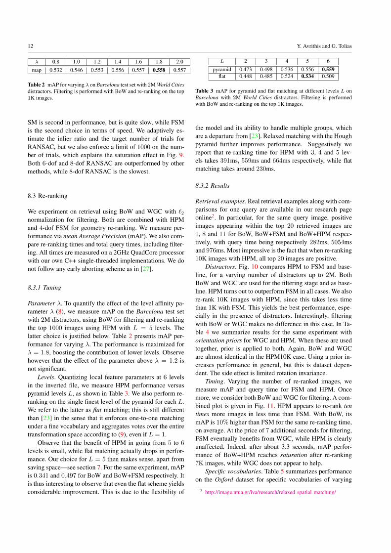
λ 0.8 1.0 1.2 1.4 1.6 1.8 2.0map 0.532 0.546 0.553 0.556 0.557 0.558 0.557

Table 2 mAP for varying λ on Barcelona test set with 2M World Citiesdistractors. Filtering is performed with BoW and re-ranking on the top1K images.

SM is second in performance, but is quite slow, while FSMis the second choice in terms of speed. We adaptively es-timate the inlier ratio and the target number of trials forRANSAC, but we also enforce a limit of 1000 on the num-ber of trials, which explains the saturation effect in Fig. 9.Both 6-dof and 8-dof RANSAC are outperformed by othermethods, while 8-dof RANSAC is the slowest.

8.3 Re-ranking

We experiment on retrieval using BoW and WGC with `2normalization for filtering. Both are combined with HPMand 4-dof FSM for geometry re-ranking. We measure per-formance via mean Average Precision (mAP). We also com-pare re-ranking times and total query times, including filter-ing. All times are measured on a 2GHz QuadCore processorwith our own C++ single-threaded implementations. We donot follow any early aborting scheme as in [27].

8.3.1 Tuning

Parameter λ. To quantify the effect of the level affinity pa-rameter λ (8), we measure mAP on the Barcelona test setwith 2M distractors, using BoW for filtering and re-rankingthe top 1000 images using HPM with L = 5 levels. Thelatter choice is justified below. Table 2 presents mAP per-formance for varying λ. The performance is maximized forλ = 1.8, boosting the contribution of lower levels. Observehowever that the effect of the parameter above λ = 1.2 isnot significant.

Levels. Quantizing local feature parameters at 6 levelsin the inverted file, we measure HPM performance versuspyramid levels L, as shown in Table 3. We also perform re-ranking on the single finest level of the pyramid for each L.We refer to the latter as flat matching; this is still differentthan [23] in the sense that it enforces one-to-one matchingunder a fine vocabulary and aggregates votes over the entiretransformation space according to (9), even if L = 1.

Observe that the benefit of HPM in going from 5 to 6

levels is small, while flat matching actually drops in perfor-mance. Our choice for L = 5 then makes sense, apart fromsaving space—see section 7. For the same experiment, mAPis 0.341 and 0.497 for BoW and BoW+FSM respectively. Itis thus interesting to observe that even the flat scheme yieldsconsiderable improvement. This is due to the flexibility of

L 2 3 4 5 6pyramid 0.473 0.498 0.536 0.556 0.559

flat 0.448 0.485 0.524 0.534 0.509

Table 3 mAP for pyramid and flat matching at different levels L onBarcelona with 2M World Cities distractors. Filtering is performedwith BoW and re-ranking on the top 1K images.

the model and its ability to handle multiple groups, whichare a departure from [23]. Relaxed matching with the Houghpyramid further improves performance. Suggestively wereport that re-ranking time for HPM with 3, 4 and 5 lev-els takes 391ms, 559ms and 664ms respectively, while flatmatching takes around 230ms.

8.3.2 Results

Retrieval examples. Real retrieval examples along with com-parisons for one query are available in our research pageonline2. In particular, for the same query image, positiveimages appearing within the top 20 retrieved images are1, 8 and 11 for BoW, BoW+FSM and BoW+HPM respec-tively, with query time being respectively 282ms, 5054msand 976ms. Most impressive is the fact that when re-ranking10K images with HPM, all top 20 images are positive.

Distractors. Fig. 10 compares HPM to FSM and base-line, for a varying number of distractors up to 2M. BothBoW and WGC are used for the filtering stage and as base-line. HPM turns out to outperform FSM in all cases. We alsore-rank 10K images with HPM, since this takes less timethan 1K with FSM. This yields the best performance, espe-cially in the presence of distractors. Interestingly, filteringwith BoW or WGC makes no difference in this case. In Ta-ble 4 we summarize results for the same experiment withorientation priors for WGC and HPM. When these are usedtogether, prior is applied to both. Again, BoW and WGCare almost identical in the HPM10K case. Using a prior in-creases performance in general, but this is dataset depen-dent. The side effect is limited rotation invariance.

Timing. Varying the number of re-ranked images, wemeasure mAP and query time for FSM and HPM. Oncemore, we consider both BoW and WGC for filtering. A com-bined plot is given in Fig. 11. HPM appears to re-rank tentimes more images in less time than FSM. With BoW, itsmAP is 10% higher than FSM for the same re-ranking time,on average. At the price of 7 additional seconds for filtering,FSM eventually benefits from WGC, while HPM is clearlyunaffected. Indeed, after about 3.3 seconds, mAP perfor-mance of BoW+HPM reaches saturation after re-ranking7K images, while WGC does not appear to help.

Specific vocabularies. Table 5 summarizes performanceon the Oxford dataset for specific vocabularies of varying

2 http://image.ntua.gr/iva/research/relaxed spatial matching/

Hough Pyramid Matching 13

103 104 105 1060.3

0.4

0.5

0.6

0.7

0.8

database size

mA

P HPM10KWGC + HPMBoW + HPMWGC + FSMBoW + FSMWGCBoW

Fig. 10 mAP comparison for varying database size on Barcelona withup to 2M World Cities distractors. Filtering is performed with BoW orWGC and re-ranking on the top 1K images with FSM or HPM, exceptfor HPM10K where BoW and WGC curves coincide.

method no distractors 2M distractorsno prior prior no prior prior

WGC+HPM10K – – 0.599 0.612BoW+HPM10K – – 0.601 0.613WGC+HPM 0.832 0.851 0.573 0.599BoW+HPM 0.832 0.837 0.558 0.565WGC+FSM 0.826 0.846 0.536 0.572BoW+FSM 0.827 – 0.497 –WGC 0.811 0.843 0.355 0.447BoW 0.808 – 0.341 –

Table 4 mAP comparison on Barcelona with and without 2M WorldCities distractors, with and without prior. Re-ranking on top 1K im-ages, except for HPM10K.

0 5 10 150.3

0.4

0.5

0.6

0

0.1

0.512 5 10 20

0

0.1

0.512 5 10 20

0

0.1

0.51

2 3

0

0.1

0.5 1 2 3

average time to filter and re-rank (s)

mA

P

WGC + HPMBoW + HPMWGC + FSMBoW + FSM

Fig. 11 mAP and total (filtering + re-ranking) query time for a varyingnumber of re-ranked images. The latter are shown with text labels nearmarkers, in thousands. Results on Barcelona with 2M World Cities dis-tractors.

method vocabulary size100K 200K 500K 700K

BoW+HPM+P 0.640 0.683 0.701 0.690BoW+HPM 0.622 0.669 0.692 0.686BoW+FSM 0.631 0.642 0.677 0.653BoW 0.545 0.575 0.619 0.614

Table 5 mAP comparison on Oxford dataset for specific vocabulariesof varying size, without distractors. Filtering with BoW and re-rankingtop 1K images with FSM and HPM. P = prior.

method Oxford Paris0 2M 0 2M

BoW+HPM10K+P – 0.418 – 0.419BoW+HPM10K – 0.403 – 0.418BoW+HPM+P 0.546 0.381 0.595 0.402BoW+HPM 0.522 0.372 0.581 0.397BoW+FSM 0.503 0.317 0.542 0.336BoW 0.430 0.201 0.539 0.282

Table 6 mAP comparison on Oxford and Paris datasets with 100Kgeneric vocabulary, with and without 2M distractors. Filtering per-formed with BoW only. Re-ranking 1K images with FSM and HPM,as well as 10K with HPM. P = prior.

size, created from all Oxford images. HPM again has supe-rior performance in all cases except for the 100K vocabulary.Our best score without prior (0.692) can also be comparedto the best score (0.664) achieved by 5-dof FSM and specificvocabulary in [27], though the latter uses a 1M vocabularyand different features. The higher scores achieved in Per-doch et al. [26] are also attributed to superior features ratherthan the matching process.

More datasets. Switching back to our generic vocab-ulary, we perform large scale experiments on Oxford andParis test sets and present results in Table 6. We considerboth good and ok images as positive examples. We haveshown the capacity of HPM to be one order of magnitudehigher than that of FSM, so it makes sense again to also re-rank up to 10K images with HPM. Furthermore, focusingon practical query times, we limit filtering to BoW. HPMclearly outperforms FSM, while re-ranking 10K images sig-nificantly increases the performance gap at large scale. Ourbest score without prior on Oxford (0.522) can be comparedto the best score (0.460) achieved by FSM in [28] with a 1Mgeneric vocabulary created on the Paris dataset.

Comparison to other models. In order to be more com-parable to previously published methods, we conduct an ex-periment using the modified version of Hessian-Affine de-tector of [26], where the gravity vector assumption is usedto estimate the dominant orientation of features for descrip-tor extraction. Similarly to [26] and [32], we switch off ro-tation for spatial matching and perform our voting schemein a pyramid of 3 dimensions. We use a 1M specific vocab-ulary trained on all images of Oxford 5K, when we test on

14 Y. Avrithis and G. Tolias

method Ox 5K Ox 105K Paris HolidaysHPM (this work) 0.789 0.730 0.725 0.790Shen et al. [32] 0.752 0.729 0.741 0.762Zhang et al. [38] 0.696 - - -[38]+RANSAC 0.713 - - -Cao et al. [7] 0.656 - 0.632 -[7]+RANSAC 0.661 - - -Perdoch et al. [26] 0.789 0.726 - 0.715FSM [27] 0.647 0.541 - -

Table 7 mAP comparison to other spatial models on Oxford 5K andOxford 105K test set. Both for our method and all other methods aspecific vobulary of size 1M is created from images of Oxford 5K.

Oxford 5K or Oxford 105K. Similarly, we use a 1M spe-cific vocabulary for Paris. We further conduct experimentson Holidays dataset. Since this includes rotated images, thegravity vector assumption does not hold and we switch backto the use of SURF features as in our previous experiments.A specific vocabulary of 200K visual words is used in thiscase as in [32].

Table 7 presents mAP performance for a number of spa-tial matching or indexing models on the Oxford 5K, Oxford105K, Paris and Holidays test sets. HPM achieves state ofthe art performance on all datasets, in fact outperforming allmethods except for Paris, where it is outperformed by Shenet al. [32], and Oxford 5K, where Perdoch et al. [26] achievethe same performance. Our query time for re-ranking 1000

images is 210ms on a single threaded implementation, whilethe one reported in [26] is 238ms on 4 cores. This time ofHPM is without the early aborting scheme of [27] or [26].The reported query time in [32] is 89ms on Oxford 5K. Bothtime and space per query are (in the worst case) linear in thedataset size for this method, as voting maps are allocated forall images having common visual words with the query.

Non-uniform quantization. Relative transformation vo-tes are not uniformly distributed in Hough space. Apart fromorientation where we use a prior, this is true also for transla-tion and scale. For instance, the distribution of relative log-scale and x parameter of translation appears experimentallyclose to the Laplacian distribution, as shown in Fig. 12 and13 respectively. If we quantize Hough space uniformly, binswill not be equally populated and votes in sparse areas willnot form groups as easily as in dense ones; and when theydo so, their affinity will be lower.

We therefore investigate normalizing distributions, i.e.,non-linear mapping of relative transformation parameters pri-or to quantization, so that vote distributions become uni-form. In particular, we model translation x, y and log-scalelog σ by Laplacian distributions, estimate their parametersvia maximum likelihood on experimental data and use thelearned CDFs to non-linearly map x, y and log σ to [0, 1].We discard assignments outside interval [0.05, 0.95], that isassignments exhibiting extreme displacement or scale change

method strength mAPBoW only - 0.341out-of-bounds removed 1.0 0.373one-to-one only 1.0 0.503HPM as in (9) 0.558

Table 8 mAP comparison on Barcelona with 2M World Cities dis-tractors, illustrating the incremental effect of enforcing voting spacebounds, enforcing one-to-one mapping, and using level-dependent cor-respondence strengths. The latter is exactly HPM.

compared to the population of our dataset. Finally, we uni-formly quantize each parameter, which is equivalent to non-uniform quantization in the original voting space.

We report results only for the combination of translationand scale normalization, since we have seen that there is noapparent benefit in other cases (e.g., when each parameteris alone. Rotation θ of the relative transformation followsa similar distribution to the one shown in [17], which wedo not normalize; we rather use the orientation prior in thiscase.

Fig. 14 shows mAP as measured on Barcelona test setfor uniform and non-uniform quantization. Quite unexpect-edly, non-uniform quantization slightly reduces performancebut it also accelerates matching considerably. Votes in sparseareas appear to increase for distractor images as well, andthis may explain why mAP is not improved. On the otherhand, matching is faster because there are more single votesin lower levels of the pyramid, and single votes do not formgroups. Non-uniform quantization is therefore a good choicefor further speed-up. However, we still use uniform quanti-zation in the remaining experiments, seeking maximum per-formance.

Effect of one-to-one-mapping. Our similarity score is aweighted sum over all correspondences between two im-ages. Correspondences with transformations falling out ofbounds (out of the HPM voting space) are discarded, as de-scribed in Section 7. Results of Table 8 show that, by just re-moving such correspondences, there is a small improvementin performance. In this case, set X of (10) includes onlyout-of-bounds correspondences, while strength w(c) is setequal to 1.0. We further enforce one-to-one mapping withour erase procedure, but still keep strengths equal to 1.0.One-to-one mapping appears to impressively improve per-formance since many false matching correspondences arenot accounted in the similarity score. Finally, using strengthsas provided by HPM (9) there is further significant improve-ment.

8.4 Re-ranking with soft assignment

We experiment on retrieval using soft assignment for visualwords [28] on the query side only [17]. We perform large

Hough Pyramid Matching 15

−2 −1 0 1 2

0

0.2

0.4

0.6

0.8

1

log σ

log σ distributionLaplacian PDFLaplacian CDF

0 0.2 0.4 0.6 0.8 1

1

1.5

2

2.5

3

·10−3

normalized log σ

normalized distribution

Fig. 12 (Left) Distribution of relative log-scale over all pairs of images of the Barcelona test set. Maximum likelihood estimation of Laplaciandistribution yields location parameter µ = 0.003 and scale parameter γ = 0.323. (Right) Normalized distribution after non-linearly mappinglog σ to [0, 1] via the Laplacian CDF.

−1,500−1,000 −500 0 500 1,000 1,500

0

0.2

0.4

0.6

0.8

1

x

x distributionLaplacian PDFLaplacian CDF

0 0.2 0.4 0.6 0.8 1500

1,000

1,500

normalized x

normalized distribution

Fig. 13 (Left) Distribution of relative x over all pairs of images of the Barcelona test set. Maximum likelihood estimation of Laplacian distributionyields location parameter µ = 139 and scale parameter γ = 251. (Right) Normalized distribution after non-linearly mapping x to [0, 1] via theLaplacian CDF.

scale experiments and compare HPM to FSM using soft as-signment with both. We use BoW for filtering in all remain-ing experiments.

Conflict detection. We compare the two methods of con-flict detection, namely based on visual word classes (ERASE)and component classes (ERASE-CC). The results are shownin Fig. 15 versus number of nearest neighbors used in softassignment. Component classes seem to outperform visualword classes in all cases, despite the fact that correct assign-ments may be discarded. In fact, the performance of the lat-ter drops eventually, which is attributed to one-to-one map-ping not being preserved. In the remaining soft assignment

experiments we only use component classes for conflict de-tection.

Nearest neighbors. We compare HPM to FSM in termsof mAP performance and re-ranking time per query ver-sus number of nearest neighbors, as shown in Fig. 16. Thetwo methods appear to converge to the same mAP as near-est neighbors increase when re-ranking 1K images. How-ever, HPM is clearly superior when re-ranking 10K images,even more so with orientation prior. HPM remains roughlyone order of magnitude faster and this is much more sig-nificant under of soft assignment than in the baseline, be-cause re-ranking time for FSM exceeds reasonable query

16 Y. Avrithis and G. Tolias

0 0.5 1 1.5 2

·104

0

2

4

6

0.460.57

0.6

0.6

0.6

0.6

0.450.56

0.59

0.6

0.6

0.6

number of re-ranked images

aver

age

time

tore

-ran

k(s

)

UniformNon-uniform

Fig. 14 Average re-ranking time versus number of re-ranked imagesfor uniform and non-uniform quantization. mAP is shown with text la-bels near markers. Results on Barcelona test set with 2M World Citiesdistractors. Filtering with BoW.

1 2 3 4 5 6 7

0.56

0.58

0.6

0.62

nearest neighbors

mA

P

EraseErase-CC

Fig. 15 Comparison of HPM conflicting assignment detection basedon visual word classes (ERASE) and component classes (ERASE-CC).mAP is given versus number of nearest neighbors in soft assignment,as measured on Barcelona test set with 2M World Cities distractors.Filtering with BoW and re-ranking top 1K images.

times above 3 nearest neighbors. The number of tentativecorrespondences is nearly linear in the number of nearestneighbors when soft assignment is performed on one sideonly [28], so it is confirmed once again that HPM is linearin the number of correspondences.

Distractors, timing. Similarly to the hard assignment case,we compare HPM and FSM for a varying number of distrac-tors up to 2M. mAP is shown in Fig. 17 where we apply softassignment with 3 nearest neighbors for all methods. Again,the benefit of HPM over FSM is higher when re-ranking 10Kimages especially with prior, in which case the gain is nearly

NN 500K 700KFSM HPM HPM+P FSM HPM HPM+P

1 0.677 0.692 0.701 0.653 0.686 0.6902 0.699 0.714 0.723 0.692 0.715 0.7193 0.707 0.716 0.724 0.701 0.721 0.7244 0.709 0.716 0.726 0.711 0.726 0.7305 0.716 0.719 0.724 0.716 0.726 0.7296 0.712 0.713 0.724 0.718 0.725 0.729

Table 9 mAP comparison on Oxford test set for specific vocabularies,without distractors. Filtering with BoW and re-ranking on the top 1Kimages with soft assignment using a varying number of nearest neigh-bors.

method Oxford Paris

BoW+HPM10K+SA+P 0.461 0.456BoW+HPM10K+SA 0.445 0.434BoW+HPM+SA+P 0.426 0.427BoW+HPM+SA 0.414 0.414BoW+FSM+SA 0.391 0.389BoW+SA 0.251 0.316

Table 10 mAP comparison on Oxford and Paris datasets with 100Kgeneric vocabulary, with 2M distractors. Filtering with BoW and re-ranking on the top 1K images with FSM and HPM, also 10K withHPM. Using soft assignment with 3 nearest neighbors.

10%. mAP versus re-ranking time for a varying number ofre-ranked images is shown in Fig. 18. Similarly to hard as-signment, HPM can re-rank one order of magnitude moreimages than FSM in the same amount of time with 10%

higher mAP. In general, all methods benefit by 7-13% bythe use of soft assignment compared to baseline BoW, butquery times become unrealistic for FSM.

Specific vocabularies. Table 9 summarizes mAP perfor-mance for specific vocabularies on Oxford test set. We usethe same vocabularies as in the hard assignment experiments.Our best score achieved on Oxford with hard assignment(0.701) now increases to 0.730. However, without distrac-tors, the gain of HPM over FSM is not as high as in the hardassignment case.

More datasets. Finally, large scale soft assignment ex-periments with a generic vocabulary and 2M distractors onOxford and Paris test sets are summarized in Table 10. Thistime the gain of HPM over FSM in mAP is roughly 5%,which becomes 7% with the prior.

9 Discussion

Clearly, apart from geometry, there are many other ways inwhich one may improve the performance of image retrieval.For instance, query expansion [10] increases recall of pop-ular content, though it takes more time to query. The lattercan be avoided by offline clustering and scene map construc-tion [1], also yielding space savings. Methods related to vi-sual word quantization like soft assignment [28] or hamming

Hough Pyramid Matching 17

1 2 3 4 5 6

0.5

0.55

0.6

0.65

0.7

nearest neighbors

mA

P

BoW+FSM+SABoW+HPM+SABoW+HPM10K+SABoW+HPM10K+SA+P

1 2 3 4 5 6

0

2

4

6

·104

nearest neighbors

aver

age

time

tore

-ran

k(m

s)

BoW+FSM+SABoW+HPM+SABoW+HPM10K+SA

Fig. 16 mAP (left) and average re-ranking time per query (right) versus number of nearest neighbors in soft assignment, measured on Barcelonatest set with 2M World Cities distractors. SA = soft assignment, P = prior.

104 105 106

0.4

0.6

0.8

database size

mA

P BoWBoW+FSMBoW+HPMBoW+SABoW+FSM+SABoW+HPM+SABoW+HPM10K+SABoW+HPM10K+SA+P

Fig. 17 mAP comparison versus database size on Barcelona with upto 2M World Cities distractors. SA = soft assignment, with 3 nearestneighbors for all methods.

embedding [17] also increase recall, at the expense of querytime and index space. Vocabulary learning [24] transfers thisproblem to the vocabulary itself, given large amounts of in-dexed images. Other priors like the gravity vector [26] alsohelp, usually at the cost of some invariance loss.

Experiments in the literature have shown that the ef-fect of such methods is additive. Comparing to our priorwork [34], we have investigated here the case of soft assign-ment and we have confirmed this finding. In fact, integratingsoft assignment has been maybe the most interesting amongother methods because it is a non-trivial problem and it hasa considerable impact on query times in general. Improvingor learning a vocabulary, query expansion or other priors are

0 10 20 30 40

0.5

0.55

0.6

0.65

0.1

1

510 15 20

0.1

1

510 15 20

0.1

0.5

1

2

0.1

0.5

11.5

2

average time to re-rank (s)

mA

P

BoW+HPM+SA3BoW+HPM+SA2BoW+FSM+SA3BoW+FSM+SA2

Fig. 18 mAP versus re-ranking time for a varying number of re-rankedimages. The latter are shown with text labels near markers, in thou-sands. Results on Barcelona with 2M World Cities distractors, usingsoft assignment with 2 and 3 nearest neighbors for both methods.

straightforward to integrate with HPM and expected to yieldfurther gain.

We have developed a very simple spatial matching al-gorithm that requires no learning and can be easily imple-mented and integrated in any image retrieval engine. It boostsperformance by allowing flexible matching and matching ofmultiple objects or surfaces. Matching is not as parameter-dependent as in other methods: λ is a relative quantity andthere is no such thing as absolute scale, fixed bin size, orthreshold parameter. Ranges and relative importance of trans-formation parameters are fixed so that they apply to mostpractical cases, while fitting the voting grid to true distribu-tions does not influence performance much.

18 Y. Avrithis and G. Tolias

By dispensing with the need to count inliers to geometricmodel hypotheses, HPM also yields a dramatic speed-up incomparison to RANSAC-based methods. It is arguably thefirst time a geometry re-ranking method is shown to reachsaturation in as few as three seconds, which is a practicalquery time. The practice so far has been to stop re-ranking ata point such that queries do not take too long, without study-ing further potential improvement using graphs like those inFigure 11.

One limitation of HPM that is shared with e.g. [23], [27],[26] is that matching depends on the precision of the lo-cal shape (e.g. scale, orientation) of the features used, apartfrom their position. On the other hand, without this informa-tion, matching is typically either not invariant (e.g. [38] isonly invariant to translation) or more costly (e.g. RANSACuses combinations of more than a single correspondence,and [32] resorts to searching for a number of scales/rotationson a discrete grid).

Another limitation may be that matching of small ob-jects is influenced by background features through the ag-gregation of votes in (9), which is exactly what gives HPMits flexibility. We expect this influence to be higher thanRANSAC-like methods that rather seek a single hypothe-sis that maximizes inliers. In fact, seeking for modes in thevoting space is still possible under our pyramid frameworkand, at an additional cost, may give precise object localiza-tion and support partial matching.

It is a very interesting question whether there is more togain from geometry indexing. Experiments on larger scaledatasets or new methods may provide clearer evidence. Ei-ther way, a final re-ranking stage always seems unavoidable,and HPM can provide a valuable tool. In fact, our first ob-jective with HPM has been for indexing and although this istoo expensive for an online query, HPM can indeed performan exhaustive re-ranking over our entire 2M distractor set ina few minutes. Further scaling up is a very challenging taskwe intend to investigate.

Another far-fetched prospect is to apply HPM to recog-nition problems. Our very assumption of inferring transfor-mations from local feature shape makes this prospect ratherlimited for object category recognition, but not necessarilyfor specific objects. Whenever feature matching becomesincreasingly ambiguous, e.g. with coarser vocabularies, re-peating or ‘bursty’ patterns [16], HPM clearly favors lowcomplexity over optimality. It would be interesting to ex-plore this trade-off. Affine covariant features and geometricmodels more complex than similarity can be another sub-ject of investigation, though flexibility of our model may notleave much space for improvement.

More can be found at our project page3, including theentire 2M World Cities dataset.

3 http://image.ntua.gr/iva/research/relaxed spatial matching

References

1. Avrithis, Y., Kalantidis, Y., Tolias, G., Spyrou, E.: Retrieving land-mark and non-landmark images from community photo collec-tions. In: ACM Multimedia. Firenze, Italy (2010) 16

2. Avrithis, Y., Tolias, G., Kalantidis, Y.: Feature map hashing: Sub-linear indexing of appearance and global geometry. In: ACM Mul-timedia. Firenze, Italy (2010) 1, 2

3. Ballard, D.: Generalizing the hough transform to detect arbitraryshapes. Pattern Recognition (1981) 2

4. Bay, H., Tuytelaars, T., Van Gool, L.: SURF: Speeded up robustfeatures. In: ECCV (2006) 10

5. Belongie, S., Malik, J., Puzicha, J.: Shape context: A new descrip-tor for shape matching and object recognition. In: NIPS, vol. 12,pp. 831–827 (2000) 2

6. Berg, A., Berg, T., Malik, J.: Shape matching and object recogni-tion using low distortion correspondences. In: CVPR (2005) 3

7. Cao, Y., Wang, C., Li, Z., Zhang, L., Zhang, L.: Spatial-bag-of-features. In: CVPR, pp. 3352–3359 (2010) 2, 14

8. Carneiro, G., Jepson, A.: Flexible spatial configuration of localimage features. PAMI pp. 2089–2104 (2007) 3, 6

9. Cheng, Y.: Mean shift, mode seeking, and clustering. PAMI 17(8),790–799 (1995) 3

10. Chum, O., Philbin, J., Sivic, J., Isard, M., Zisserman, A.: Totalrecall: Automatic query expansion with a generative feature modelfor object retrieval. In: ICCV (2007) 16

11. Enqvist, O., Josephson, K., Kahl, F.: Optimal correspondencesfrom pairwise constraints. In: ICCV (2009) 3

12. Fischler, M., Bolles, R.: Random sample consensus: A paradigmfor model fitting with applications to image analysis and auto-mated cartography. Communications of the ACM 24(6), 381–395(1981) 2

13. Grauman, K., Darrell, T.: The pyramid match kernel: Efficientlearning with sets of features. Journal of Machine Learning Re-search 8, 725–760 (2007) 1, 3, 5, 7

14. Indyk, P., Thaper, N.: Fast image retrieval via embeddings. In:Workshop on Statistical and Computational Theories of Vision(2003) 3

15. Jegou, H., Douze, M., Schmid, C.: Hamming embedding and weakgeometric consistency for large scale image search. In: ECCV(2008) 10

16. Jegou, H., Douze, M., Schmid, C.: On the burstiness of visual ele-ments. In: CVPR (2009) 18

17. Jegou, H., Douze, M., Schmid, C.: Improving bag-of-features forlarge scale image search. IJCV 87(3), 316–336 (2010) 1, 2, 3, 8,10, 11, 14, 16

18. Jiang, H., Yu, S.X.: Linear solution to scale and rotation invariantobject matching. In: CVPR (2009) 3

19. Lazebnik, S., Schmid, C., Ponce, J.: Beyond bags of features: Spa-tial pyramid matching for recognizing natural scene categories. In:CVPR, vol. 2, p. 1 (2006) 3

20. Leibe, B., Leonardis, A., Schiele, B.: Robust object detection withinterleaved categorization and segmentation. IJCV 77(1), 259–289 (2008) 2

21. Leordeanu, M., Hebert, M.: A spectral technique for correspon-dence problems using pairwise constraints. In: ICCV, vol. 2, pp.1482–1489 (2005) 1, 3, 4, 6, 11

22. Lin, Z., Brandt, J.: A local bag-of-features model for large-scaleobject retrieval. ECCV pp. 294–308 (2010) 3

23. Lowe, D.: Distinctive image features from scale-invariant key-points. IJCV 60(2), 91–110 (2004) 1, 2, 3, 9, 12, 18

24. Mikulik, A., Perdoch, M., Chum, O., Matas, J.: Learning a finevocabulary. In: ECCV (2010) 16

25. Olsson, C., Eriksson, A., Kahl, F.: Solving large scale binaryquadratic problems: Spectral methods vs. semidefinite program-ming. In: CVPR (2007) 4

Hough Pyramid Matching 19

26. Perdoch, M., Chum, O., Matas, J.: Efficient representation of localgeometry for large scale object retrieval. In: CVPR (2009) 13, 14,16, 18

27. Philbin, J., Chum, O., Isard, M., Sivic, J., Zisserman, A.: Objectretrieval with large vocabularies and fast spatial matching. In:CVPR (2007) 1, 2, 3, 10, 11, 12, 13, 14, 18

28. Philbin, J., Chum, O., Sivic, J., Isard, M., Zisserman, A.: Lost inquantization: Improving particular object retrieval in large scaleimage databases. In: CVPR (2008) 3, 8, 10, 13, 14, 15, 16

29. Raguram, R., Frahm, J.M.: Recon: Scale-adaptive robust estima-tion via residual consensus. In: ICCV (2011) 3

30. Sahbi, H., Audibert, J.Y., Rabarisoa, J., Keriven, R.: Context-dependent kernel design for object matching and recognition. In:CVPR (2008) 3

31. Scott, G., Longuet-Higgins, H.: An algorithm for associating thefeatures of two images. Proceedings of the Royal Society of Lon-don 244(1309), 21 (1991) 3

32. Shen, X., Lin, Z., Brandt, J., Avidan, S., Wu, Y.: Object retrievaland localization with spatially-constrained similarity measure andk-nn re-ranking. In: CVPR. IEEE (2012) 3, 13, 14, 18

33. Sivic, J., Zisserman, A.: Video Google: A text retrieval approachto object matching in videos. In: ICCV, pp. 1470–1477 (2003) 1,10

34. Tolias, G., Avrithis, Y.: Speeded-up, relaxed spatial matching. In:ICCV (2011) 3, 17

35. Vedaldi, A., Soatto, S.: Quick shift and kernel methods for modeseeking. In: ECCV (2008) 3

36. Vedaldi, A., Soatto, S.: Relaxed matching kernels for robust imagecomparison. In: CVPR (2008) 3

37. Wu, Z., Ke, Q., Isard, M., Sun, J.: Bundling features for large scalepartial-duplicate web image search. In: CVPR (2009) 2

38. Zhang, Y., Jia, Z., Chen, T.: Image retrieval with geometry-preserving visual phrases. In: CVPR, pp. 809–816. IEEE (2011)2, 14, 18

39. Zhou, W., Lu, Y., Li, H., Song, Y., Tian, Q.: Spatial coding forlarge scale partial-duplicate web image search. In: ACM Multi-media. Firenze, Italy (2010) 2