hotelling trace criterion as a figure of merit for the...

Research Article

Received: 7 July 2014, Revised: 6 December 2014, Accepted: 10 December 2014, Published online in Wiley Online Library: 25 February 2014

(wileyonlinelibrary.com) DOI: 10.1002/cem.2696

Hotelling trace criterion as a figure of merit forthe optimization of chromatogram alignment

Edward J. Soaresa*, Gopal R. Yallaa, John B. O’Connora,b, Kevin A. Walsha

and Amber M. Huppb

We present a methodology for optimization of chromatogram alignment using a class separability measure calledthe Hotelling trace criterion (HTC). This metric is a multi-class distance measure that accounts for within-classand between-class variation. We chose the correlation optimized warping algorithm as our alignment method andused the HTC to judge the effectiveness of the alignment based on algorithm parameters called segment lengthand max warp.Biodiesel feedstock samples representing classes of soy, canola, tallow, waste grease, and hybrid were used in ourexperiments. Fatty acid methyl esters in each biodiesel were separated using gas chromatography-mass spectroscopy.The entire data set was baseline corrected, aligned, normalized, and mean-centered prior to principal components(PCs) analysis. The aligned, baseline corrected data sets were used to compute a figure of merit called warping effect,while the PC-transformed data sets were used to evaluate the HTC. The segment length and max warp parametersthat maximized the warping effect and/or HTC were then determined. Scores plots of pairs of PCs, along with 95%confidence ellipses, were created and analyzed.The results demonstrated that the parameters derived from maximizing the HTC more effectively aligned the data,as evidenced by better clustering of the biodiesels in the scores plots. This behavior was robust to the number of PCsused in the computation of the HTC. We conclude that the HTC is an objective measure of alignment quality that allowsfor optimal class separability and can be applied to optimize other methods of chromatogram alignment. Copyright© 2015 John Wiley & Sons, Ltd.

Keywords: Hotelling trace criterion; correlation optimized warping; principal components analysis; gas chromatography;biodiesel

1. INTRODUCTION

Complex chromatographic data can be challenging to analyzebased on the sheer number of chemical components in a sam-ple. Chemometric methods such as principal component analysishave been widely used to determine interesting trends from com-plex data sets [1–13]. Researchers have used several methodsincluding extracting peak areas [1,4,5] as well as using the full,raw data set [8,14,15]. Extracting retention time peak areas canbe straightforward. However, typically, a judgment of the num-ber and type of chemical components must be made by the user.Using the raw data set does not require such a judgment, as everydata point in the sample is investigated. However, this methodrequires more sophisticated data processing as every sample inthe set must be aligned prior to any subsequent chemometricanalysis [16,17]. With gas chromatography (GC), normal fluctu-ations occur in both peak height (because of variation in themanually injected volume) and retention time (because of slightdifferences in oven temperature, analyte interaction on column,etc.). Thus, without retention time alignment, the trends that aredetermined using chemometric methods of analysis could beskewed or meaningless.

Several authors have proposed alignment algorithms for GCmeasurements that operate on the entire chromatogram. Wangand Isenhour [18] presented a dynamic programming approach

to time warp data derived from gas chromatography/Fouriertransform infrared/mass spectroscopy experiments using a dis-tance measure to produce an optimal match. This dynamic timewarping (DTW) algorithm requires setting a window constraintand local constraint on the number of one-direction consecu-tive moves that can be made. Vest Nielsen et al. [14] introduceda correlation optimized warping (COW) method that uses piece-wise stretching and compression of segments of the data, as wellas the linear correlation between matching segments, to opti-mally align two chromatographic profiles. This algorithm requiresthe setting of two parameters: segment length, which is thefixed length used to divide up each chromatogram and max-imum warp, which is the largest amount of stretching and/orcompression a particular segment may undergo. Pierce et al.

* Correspondence to: Edward J. Soares, Department of Mathematics and Com-puter Science, College of the Holy Cross, 1 College Street, Worcester, MA,01610, USA.E-mail: [email protected]

a E. J. Soares, G. R. Yalla, J. B. O’Connor, K. A. WalshDepartment of Mathematics and Computer Science, College of the Holy Cross,Worcester, MA 01610, USA

b J. B. O’Connor, A. M. HuppDepartment of Chemistry, College of the Holy Cross, Worcester, MA 01610, USA

20

0

J. Chemometrics 2015; 29: 200–212 Copyright © 2015 John Wiley & Sons, Ltd.

Optimizing chromatogram alignment using HTC

[19] presented a variant of local retention time alignment calledpiece-wise alignment. Like COW, piece-wise alignment uses asegment length parameter to divide up the chromatogram andthen shifts segments of the data to find the optimal correlationbetween the segments. However, it does not incorporate stretch-ing and/or compression thus saving computation time. Severalauthors [20–22] have tested and compared the effectiveness ofalignment algorithms including COW and DTW using experimen-tal data, although none have incorporated objective measures ofalignment quality assessment into their analysis.

Most algorithms that align the entire chromatogram requirethe selection of one or more input parameters and so a nat-ural question arises regarding the selection of a "best" set ofparameters that will produce an optimal alignment of the data.To perform such an optimization, one needs to define a per-formance metric that objectively quantifies the quality of thealignment. Pierce et al. [19] define a measure of alignment qualitycalled degree of class separation, which is the ratio of the Euclideandistance between two principal component (PC) class means withthe square root of their average variances. However, this quan-tity is only based on data from two of the classes, and it doesnot account for the linear correlation that may exist betweenthe PCs for a particular class. Sinkov and Harynuk [23] use clus-ter resolution as their criterion for class separability, which is themaximum confidence limit for which confidence ellipses fromtwo different classes do not overlap. For applications in whichmore than two classes are present, a value for cluster resolu-tion is obtained from each possible pair of classes, and then, theproduct of these is computed. While this measure may accountfor separation between all of the classes, it does not measuretheir separability simultaneously. Skov et al. [15] define a mea-sure called warping effect, which measures both the degree ofsimilarity in the aligned data set and the amount of distortionthe alignment has introduced. Because the data set may containdifferent types of samples, we may want to preserve these differ-ences post-alignment. But, the warping effect measure may notserve to value difference preservation.

In this work, we investigate the use of the Hotelling trace cri-terion (HTC) [24] as a metric to determine the parameters thatserve to optimally align GC data. The HTC is an omnibus mea-sure of class separability [25] that incorporates both within-classand between-class variations and is the multi-class extension ofthe Mahalanobis distance [26]. Researchers have previously usedthe HTC as a quality metric for feature enhancement in imageprocessing [27] and imaging system optimization [28].

We evaluated the suitability of the HTC using data from severalbiodiesels derived from various feedstocks (soybean oil, canolaoil, waste cooking grease, and animal tallow) and analyzed usinggas chromatography with mass spectrometry. The COW algo-rithm is employed as an alignment tool for the data; however, anymethod that requires input parameters may be employed. Wecompare the effectiveness of the HTC as a figure of merit to thewarping effect metric of Skov et al. [15].

2. THEORY

2.1. Nomenclature and terminology

A measurement vector is used to represent a sample chro-matogram. The time axis refers to the direction over which chem-ical components elute and along which warping and alignmentoccur. We use italics for scalars (i.e., a), lowercase bold for col-

umn vectors (i.e., a), uppercase bold for matrices (i.e., A), andsuperscript t to denote matrix/vector transpose. Data matrices arealso denoted by uppercase bold (i.e., X), where the row index ncorresponds to sample chromatogram, and the column index mcorresponds to retention time.

We assume a sample chromatogram has M elements (reten-tion times), and that there are a total of N sample chromatogramsin a data set. Furthermore, we assume that each sample chro-matogram belongs to one of K distinct classes, where there areNk sample chromatograms in the kth class, with N1 + N2 + � � � +NK = N. Thus, the quantity xknm represents the measurementof peak height at retention time index m in the nth samplechromatogram that belongs to the kth class, while the vectorxkn is vector of measurements of the nth chromatogram fromthe kth class.

Raw sample chromatograms that undergo some kind of pro-cessing or correction will have the processing method denotedby a superscript in parentheses. Thus, a chromatogram that has

processed with correction method Q will be denoted by x(Q)kn .

2.2. Baseline correction

Before a sample chromatogram can be aligned and transformedusing principal components, baseline correction (BC) should beperformed, as baseline shifts can introduce artificial variabilityin peak height. In our study, the baseline shape of each chro-matogram exhibited a non-linear increase as a function of reten-tion time. We employed a variation of the baseline correctionmethod of Eilers and Boelens [29] to correct for this curvature.

The method uses asymmetric least squares smoothing todetermine a baseline vector b0 that minimizes

f (b0) = kwt(b0 – xkn)k2 + �kDb0k2 (1)

where k � k is the Euclidean norm, w is a vector of weights, � is arelaxation parameter, and D is a second-difference matrix (i.e., atridiagonal matrix with value 2 on the main diagonal, value –1 onthe first sub-diagonals above and below the main diagonal, andthe rest of the elements zero). The first term of f ensures b0 is agood fit to xkn, while the second term ensures that b0 is smooth.The parameter � controls the relative importance of these twoproperties: larger � results in a smoother baseline and smaller �results in a better fit to xkn. The weights w are used to prioritizefitting certain points in xkn or to selectively ignore points in xkn.

Eilers and Boelens give an iterative algorithm for choosing suit-able weights. For our purposes, a non-iterative approach sufficed,as follows. Intuitively, we should assign zero weight to points inxkn near peaks in the chromatogram, because peaks have largedeviations from the baseline. To identify peaks, let us assume

xkn = s + b + � (2)

where s is the non-random true peak height, b is the true non-random baseline to be estimated, and � denotes the randomerror. Furthermore, we assume that s is sparse (i.e., usually 0) withnarrow, large deviation peaks of a fixed maximum width, b issmooth, and each component of � is normally distributed with asmall standard deviation �� .

Let mi be the median vector of elements in xkn over someappropriately-sized window of size T centered at time index i.Then, m � b, because the median is a robust measure of centraltendency and xkn � b + �, except for some outliers due to peaks

J. Chemometrics 2015; 29: 200–212 Copyright © 2015 John Wiley & Sons, Ltd. wileyonlinelibrary.com/journal/cem

20

1

E. J. Soares et al.

in s. Furthermore, the median absolute deviation is a consistentestimator of �� , with �� 1.4826 �median(jxkn – mj).

We consider each xkni that lies outside an envelope defined bymi ˙ 2�� as an outlier due to peaks in s. So, we choose weightwi = 0 if xkni falls outside this envelope and choose weightwi = 1 otherwise. An asymmetric least squares fitting using theseweights is then performed to obtain b0, an estimate for the truebaseline b. Subtracting the baseline yields a baseline-corrected

chromatogram x(BC)kn

x(BC)kn = xkn – b0 � s + � (3)

2.3. Correlation optimized warping

Prior to chemometric analysis, the full chromatograms need to bealigned, as small shifts in chromatographic profiles with respectto retention time can cause severe variations in chemometricanalyses [16]. The COW algorithm [14] was chosen to align ourdata. This method is based on aligning a sample chromatogramto a target chromatogram (i.e., a reference sample) by piece-wisestretching and/or compression of segments of the data, in com-bination with linear interpolation and optimization with regardto the linear correlation coefficients between corresponding seg-ments in the sample and target chromatograms. The detailsof the implementation of COW can be found in Vest Nielsenet al. [14]. Tomasi et al. [21] provide a conceptual example ofthe underlying algorithm. The COW algorithm uses two inputparameters that specify the fixed size of each segment, and themaximum amount of warping each segment may undergo. Wewill refer to them as segment length and max warp, respectively.The quality of the alignment depends heavily on the selection ofthese parameters.

The choice of the reference sample is important, as it serves asthe basis of alignment for all of the other samples. In their work,Skov et al. [15] discuss a number of approaches that can be takento choose this target chromatogram. In particular, they refer toa quantity called the similarity index (SI) as a figure of merit fordetermining the best reference sample. To compute SI for the

jth baseline-corrected chromatogram in the k0th class, x(BC)k0j , we

take the product of the absolute values of the sample correla-tion coefficients between this chromatogram and all of the otherchromatograms in all of the classes

SIj =NY

n = 1 , n¤j

|r�

x(BC)k0j , x(BC)

kn

�| (4)

The chromatogram that possesses the highest SI is regarded asbeing the most similar to all of the other chromatograms. Thus, itis chosen as the target for alignment. One then applies the COW

algorithm to each baseline-corrected chromatogram x(BC)kn using

this reference sample to produce an aligned, baseline-corrected

chromatogram x(BC, COW)kn .

2.4. Data transformation

After baseline correction and alignment, each chromatogram

x(BC, COW)kn should be normalized to account for variations in injec-

tion volume. To accomplish this, the intensity at each retentiontime was summed to define a total area under the nth chro-

matogram in the kth class

Akn =MX

m = 1

x(BC, COW)knm (5)

and the average total area of all of the chromatograms in the dataset was also computed

NA =1

N

KXk = 1

NkXn = 1

Akn (6)

Each component of a given chromatogram was subsequentlydivided by its total area Akn so that each normalized chro-matogram had a unit area. To return the data to the same order ofmagnitude before normalization, each chromatogram was scaledby the average total area previously computed. These steps canbe accomplished via

x(BC, COW, NORM)kn =

NA

Akn� x(BC, COW)

kn (7)

Mean-centering (MC) of each chromatogram is often doneprior to chemometric analysis in order to shift the relative locationof the data to the origin. Centering the data preserves the relativeinter-sample relationships and allows one to more easily considerrelationships between samples [30]. After area normalization andscaling, the sample grand mean chromatogram is computed

Nx(BC, COW, NORM) =1

N

KXk = 1

NkXn = 1

x(BC, COW, NORM)kn (8)

and then subtracted from each sample chromatogram to com-pute a mean-centered, aligned, and baseline-corrected chro-

matogram x(BC, COW, NORM, MC)kn

x(BC, COW, NORM, MC)kn = x(BC, COW, NORM)

kn – Nx(BC, COW, NORM) (9)

In order to more easily identify differences in the chromato-graphic profiles of the samples, the dimensionality of the chro-matograms must be reduced while not eliminating importantinformation contained in the data. The principal componentstransformation [26] is used for this purpose. It is a multivariatestatistical technique that reorders the large numbers of possiblycorrelated measurements into a smaller set of uncorrelated fea-tures, called PCs. More importantly, these PCs still retain mostof the variation in the original data set [30,31]. Ideally, only theimportant discriminating characteristics of the original data areretained within a small set of features, from which natural clustersof similar samples can be identified.

Let S represents the sample covariance matrix of the entire setof processed sample chromatograms with eigen decomposition[26,32,33] given by

S = UƒUt (10)

where U is the orthogonal matrix whose columns are theeigenvectors (loadings) of S, and ƒ is the diagonal matrix ofeigenvalues that represent the variances related to each PCvariable. Then, ykn, the vector of PCs for sample chromatogram

x(BC, COW, NORM, MC)kn is computed via the matrix transformation

20

2

wileyonlinelibrary.com/journal/cem Copyright © 2015 John Wiley & Sons, Ltd. J. Chemometrics 2015; 29: 200–212


ykn = Utx(BC, COW, NORM, MC)kn (11)

Each PC is a linear combination of the original measurements.Furthermore, only the first few elements of ykn will likely con-tain useful information for the purpose of discrimination betweensample classes.

2.5. Optimization criteria

As previously stated, the COW algorithm requires two user-defined input parameters: segment length and max warp. Theselection of these parameters affects how well the alignment isperformed. In order to identify the best parameter values, wehave to decide on a figure of merit for judging the effectiveness(or quality) of the alignment.

2.5.1. Warping effect

Some authors have conjectured that making the entire set ofchromatograms as similar as possible while retaining peak shapeand area should be the goal of alignment. Skov et al. [15] havedefined a figure of merit to quantify this similarity called warp-ing effect, which is the sum of two quantities: simplicity and peakfactor. Simplicity is related to the rank of the data matrix for thealigned, baseline-corrected chromatograms. A data matrix withrank 1 means that there is only one linearly independent sam-ple chromatogram, and that all of the other chromatograms arescalar multiples of the first. Thus, higher values for simplicitymeans that the chromatograms are more similar, thus reflectingthat they are better aligned.

If X is the data matrix for the aligned, baseline-corrected chro-matogram profiles, then simplicity is defined to be [15]

simplicity =RX

r = 1

0B@SVD

0B@X/

vuuutKX

k = 1

NkXn = 1

MXm = 1

x2knm

1CA

1CA

4

(12)

where r is the singular value index and division by the total sumof the elements in X scales the singular values so that they sum to1. Values of simplicity closer to 1 indicate that the chromatogramsare better aligned, while values closer to 0 correspond to devia-tions from ideal alignment.

The second quantity, peak factor, is intended to measure howmuch the shape and peak area of chromatograms have beenchanged by the warping. If we define

ckn = |k x(BC, COW)

kn k – k x(BC)kn k

k x(BC)kn k

(13)

as the relative error between a baseline-corrected chromatogrambefore alignment and after alignment, then peak factor can becomputed as [15]

peak factor =1

N

KXk = 1

NkXn = 1

�1 – min

�ckn, 1

�2�

(14)

When alignment distorts a sample, ckn will be large, and so itscontribution to peak factor will be zero. However, when the sam-ple stays relatively unchanged, ckn will be small and thus willcontribute a 1/N to the sum. Thus, better alignment corresponds

Figure 1. Representative total ion chromatograms from each fuel classshowing separation of FAME components for m/z = 20 to 400 for biodieselfuels produced from different feedstock types.

1 2 3 4 5 6 7 8 9 100

10

20

30

40

50

60

70

80

90

100

110

EIGENVALUE INDEX

CU

MU

LAT

IVE

% T

OT

AL

VA

RIA

NC

E

CUMULATIVE % TOTAL VARIANCE WITH 95% CI

Figure 2. A plot of median cumulative percent total variation versuseigenvalue index, along with 95% confidence bounds.

to larger values for simplicity and peak factor and consequentlyfor warping effect.

2.5.2. Hotelling trace criterion

For a set of chromatograms that contains samples from differentclasses, we would like to identify those differences. Therefore, it isdesirable to remove variation in peak location along the time axisbut retains variation in peak height. Simplicity is a global measureof similarity between all of the samples that does not quantifyclass separability, and so maximizing it might not serve to identifythe segment length and max warp parameters that best retainthese differences. Ideally, we would like to use a measure thatreflects our ability to discriminate between the different classesof biodiesels.

When there are two multivariate populations present, the sam-ple Mahalanobis distance [26] gives a numerical measure of thedistance between the distributions. However, we have K > 2multivariate populations to consider. In this scenario, the HTC


20

3

E. J. Soares et al.

[24,27,28], which is the multi-class extension of the Mahalanobisdistance, provides us with this same numerical measure of dis-tribution separability. Like the Mahalanobis distance, the HTCincorporates both within-class and between-class variations inthe data set. We evaluated the HTC based on the PCs of ourtransformed sample chromatograms.

Let zkn = (ykn1, ykn2, � � � , yknL)t denotes the L � 1 vector cor-responding to the first L PCs of ykn, where ykn is the nth PCvector belonging to the kth class. The sample mean vector Nzkand sample covariance matrix Sk for the kth class are givenrespectively by

Nzk =1

Nk

NkXn = 1

zkn (15)

and

Sk =1

Nk – 1

NkXn = 1

�zkn – Nzk

� �zkn – Nzk

�t (16)

Furthermore, we define the grand mean vector of all of theclasses as

NNz =KX

k = 1

Pk Nzk (17)

where Pk = Nk/N is the probability of occurrence for class k. Usingthese quantities, we define the within-class scatter matrix Swc as

Swc =KX

k = 1

PkSk (18)

and the between-class scatter matrix Sbc as

Sbc =KX

k = 1

Pk�Nzk – NNz

� �Nzk – NNz

�t(19)

The matrix Swc quantifies the average multi-dimensional disper-sion within each class about the class mean, while Sbc quantifiesthe average multi-dimensional dispersion between each classmean and the grand mean. The HTC is then defined to be

J = tr�

S–1wcSbc

�(20)

where tr(�) denotes the trace of the matrix argument. Largevalues of J correspond to better class separability. Smallerwithin-class variation increases the value of J, as does largerbetween-class variation.

Thus, we seek to use the HTC as our optimization metric, inorder to identify the values of segment length and max warp

needed for COW alignment that will maximize the separability ofthe different classes of biodiesels. It is important for the reader tonote that our computation of the HTC is dependent on the num-ber of PCs (L) that we include in zkn. In fact, as L increases, thevalue of the HTC will also increase.

3. EXPERIMENTAL METHODS

3.1. Chemicals

Biodiesel fuel samples were obtained from various manufactur-ers throughout the USA (Minnesota Soybean Processors (soybeanbiodiesel, Minn Soy 2010, 2011), Western Dubuque Biodiesel(soybean biodiesel, Iowa Soy 2010), Iowa Renewable Energy(soybean biodiesel, canola biodiesel, tallow biodiesel, IRE Soy,canola, Tallow 2012), National Institute of Standards and Tech-nology (Standard Reference Material (SRM) 2772, soy SRM, soy-bean biodiesel from Ag Processing Inc. and SRM 2773, animalSRM, tallow/soybean biodiesel mixture from Smithfield BioEn-ergy LLC), ADM Company (canola biodiesel, ADM Canola 2010,2011), TMT Biofuels (waste grease biodiesel, Waste Grease 2010,2011), Texas Green Manufacturing (beef tallow biodiesel, TexasTallow 2010, 2012), and Keystone Biofuels (unknown biodiesel,Keystone 2010)) and were stored in their original shipping con-tainer at 4 ıC. Prior to dilution, each biodiesel was graduallywarmed to room temperature and was inverted multiple times toensure homogeneity. An amount of 1 mL of each biodiesel sam-ple was diluted to 100 mL total volume with methylene chloride(BDH chemicals distributed by VWR, West Chester, PA, USA), and1 mL of 0.30 M tridecanoic acid methyl ester (Fluka) was addedto a 50-mL volumetric flask and was diluted to volume with the100:1 biodiesel. Tridecanoic acid methyl ester (C13) was cho-sen as an internal standard as it was not present in any of thebiodiesel samples originally. All diluted biodiesel solutions werestored in amber bottles at 4 ıC and were gradually warmed toroom temperature prior to analysis.

3.2. Instrumentation

Separations were performed using an Agilent 6890 gaschromatograph coupled with an Agilent 5937 mass spec-trometer (Agilent Technologies, Santa Clara, CA, USA) andhave been presented in detail previously [34]. The gas chro-matography with mass spectrometry was equipped with apolyethylene glycol fused-silica capillary column of dimensions30 m� 0.25 mm� 0.25�m (ZB-WAXplus, Phenomenex). Theoven temperature was optimized to ensure baseline resolution ofall Fatty acid methyl esters (FAME) in a 37-component FAME stan-dard (Supelco) and was as follows: 60 ıC (hold 2 min) to 150 ıCat 13 ıC/min to 230 ıC at 2 ıC/min. High purity helium was used

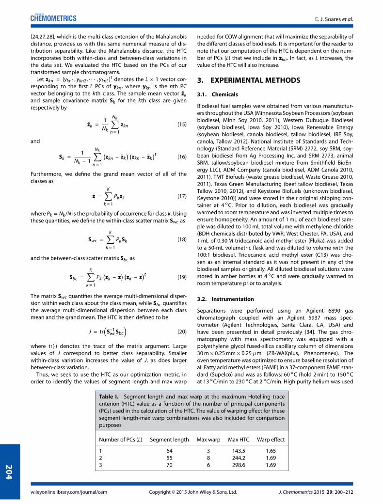
Table I. Segment length and max warp at the maximum Hotelling tracecriterion (HTC) value as a function of the number of principal components(PCs) used in the calculation of the HTC. The value of warping effect for thesesegment length-max warp combinations was also included for comparisonpurposes

Number of PCs (L) Segment length Max warp Max HTC Warp effect

1 64 3 143.5 1.652 55 8 244.2 1.693 70 6 298.6 1.692

04



Figure 3. Two-dimensional (2D) density plots of simplicity, peak factor, and warping effect. Maximum values for both simplicity and warping effectoccurred for segment length-max warp of (26,15).

as a carrier gas at a nominal flow rate of 1.5 mL/min. Each samplewas injected via syringe (1�L injected from 10�L syringe, Hamil-ton Company) with a split ratio of 50:1. The inlet and transfer linetemperatures were held at 250 ıC and 280 ıC, respectively. Anelectron-impact ionization source was utilized with a quadrupolemass analyzer operated in full-scan mode (m/z 20,300) with asampling rate of 4.94 scans/s. The mass spectrometer sourceand quadrupole were held at 230 ıC and 150 ıC, respectively.

FAME identification was performed using the mass spectralibrary (National Institute of Standards and Technology massspectral search program version 2.0a, Gaithersburg, MD, USA) aswell as retention time comparison to the FAME standard. Repre-sentative total ion chromatograms from each fuel class showingseparation of FAME components for m/z = 20 to 400 for biodieselfuels produced from different feedstock types are shownin Figure 1.


20

5

E. J. Soares et al.

Figure 4. Two-dimensional (2D) density plots of Hotelling trace criterion (HTC). Maximum values occurred for segment length-max warp combinationsof (64,3) using one principal component (PC), (top), (55,8) using two PCs (middle), and (70,6) using three PCs (bottom).

3.3. Data processing

Total ion chromatograms were extracted from Chemstation using

a macro developed by Infometrix (Bothell, WA, USA). All chro-matograms were first baseline corrected using a python imple-mentation of the method previously described with window sizeT = 1000, a maximum peak detection width of 20, and relaxationparameter � = 107. In addition, portions of the chromatogram

that did not contain chemical information (0–5 min and 40.37–48.92 min) were removed prior to further chemometric analysis,resulting in 10,500 sample values in each chromatogram.

Next, the chromatograms were aligned using a MATLAB imple-mentation of the COW algorithm (http://www.models.life.ku.dk/algorithms) under the same combinations of segment length-max warp as seen in Skov et al. [15]. Segment lengths rangedfrom 10 through 70. For segment lengths between 10 and 19

20

6


http://www.models.life.ku.dk/algorithms

http://www.models.life.ku.dk/algorithms


(inclusive), max warp was equal to segment length minus 4.For segment lengths greater than or equal to 20, max warp wasfixed at 15. This produced 870 total aligned, baseline-correcteddata sets. The reference sample, a waste grease, was determinedas the sample chromatogram that produced the largest SI.

The 870 aligned, baseline-corrected data sets were then nor-malized and scaled as previously described using MATLAB scriptswritten in-house. The PC transform was then computed for eachdata set and was applied to each chromatogram to gener-ate the corresponding PC scores using MATLAB’s statistics tool-box. Only PC information regarding the 10 largest eigenvalueswas retained.

After all of the data had been fully processed, the figuresof merit were tabulated. For each of the 870 aligned, baseline-corrected data sets, the value of warping effect was com-puted. Because each data file correspondeds to COW processingwith a particular combination of segment length-max warp, wearranged the values of warping effect into a two-dimensional(2D) density plot, with segment length along the horizontal axisand max warp along the vertical axis. Furthermore, for each of

the 870 PC-transformed data files, the HTC was computed asa function of the number of PCs L. There were five classes ofbiodiesels: soy (six different samples), canola (three different sam-ples), tallow (three different samples), waste grease (two differentsamples), and hybrid (one sample – 15% soy and 85% tallow) witheach sample measured in three different runs. The HTC valuesalso corresponded to COW processing with a particular segmentlength-max warp, so the HTC values were similarly arranged into2D density plots. MATLAB scripts to perform these computa-tions were written in-house and are available from the authorsupon request.

The maximum warping effect was found to be 1.74, obtainedusing a segment length-max warp pair of (26,15). The readershould also note that processing with this parameter combina-tion produced the following values for the HTC: 31.3 (L = 1), 55.9(L = 2), and 104.6 (L = 3). We chose L = 3 as the maximum num-ber of PCs to include in the calculation of HTC, as over 90% of thecumulative percent total variation is accounted for when L = 3, ascan be seen in Figure 2. We also found the maximum HTC valueas a function of L and determined the combinations of segment

Figure 5. Scatter plots of principal component (PC)2 versus PC1 for combinations of segment length-max warp (26,15) (top left), (64,3) (top right), (55,8)(bottom left), and (70,6) (bottom right). Classes displayed are as follows: soy (ı), canola (˘), tallow (�), waste grease (*), and hybrid (+).


20

7

E. J. Soares et al.

length-max warp that produced them. It should be noted thatthese combinations changed with L. These results can be seenin Table I.

Two-dimensional scores plots of combinations of the first,second, and third PCs of the data sets corresponding to seg-ment length-max warp combinations of (26,15), (64,3), (55,8),and (70,6), were then created. Confidence ellipses were alsodetermined using a method similar to that described in [35]and implemented by Schwarz [36]. These were included on thescores plots.

4. RESULTS AND DISCUSSION

The results of our investigation into the optimization of theCOW algorithm parameters can be seen in Figures 3–7 andTables II–III. Figure 3 displays 2D density plots of simplicity, peakfactor, and warping effect, as functions of segment length-maxwarp. The analogous 2D density plots of the HTC, using one, two,or three PCs in its computation are given in Figure 4. 2D scoresplots of pair-combinations of the PCs, along with corresponding95% confidence ellipses are displayed in Figure 5 (PC2 vs PC1), inFigure 6 (PC3 vs PC1), and in Figure 7 (PC3 vs PC2), for the four

groupings of segment length-max warp discussed in the Exper-imental Methods section. Table II lists the Euclidean distancesbetween each pair of class means, while Table III lists the ratiosof the standard deviations along the principal axes of each class,where the numerator is the class standard deviation of the dataderived from maximizing the HTC, while the denominator is theclass standard deviation of the data derived from maximizing thewarping effect.

Considering Figure 3, the density plot for peak factor (middle)is fairly uniform. In fact, peak factor values ranged from 0.9934to 1.0. Because of this narrow range, the density plot for warpingeffect was approximately the same as the density plot for sim-plicity plus a constant factor. We note that maximum values ofboth simplicity and warping effect occurred at segment length-max warp combination (26,15). However, the range of values ofboth of these figures of merit is small. Therefore, based only onthese density plots, it is difficult to determine if the segmentlength-max warp parameters corresponding to the maximum willresult in any meaningful differences in discriminability betweenthe classes.

This limited range in values is not seen for the HTC figureof merit. In Figure 4, the corresponding 2D density plots for

Figure 6. Scatter plots of principal component (PC)3 versus PC1 for combinations of segment length-max warp (26,15) (top left), (64,3) (top right), (55,8)(bottom left), and (70,6) (bottom right). Classes displayed are as follows: soy (ı), canola (˘), tallow (�), waste grease (*), and hybrid (+).

20

8



the HTC, as a function of the segment length-max warp com-bination, are given. The broader range in values can be seenvisually and by examining the color bars in each plot. As previ-ously noted, maximum values occurred for segment length-maxwarp combinations of (64,3) using one PC, (55,8) using two PCs,and (70,6) using three PCs. Two important observations can benoted. First, the HTC values exhibit greater variation in magni-tude as compared with the measures of simplicity and warpingeffect. Thus, there should be substantive differences in class sep-arability when using different combinations of segment length-max warp. Second, the magnitude of the HTC increases as thenumber of PCs used in the calculation increases. Thus, the usermust decide to either use a specific number of PCs in the cal-culation of the HTC or to evaluate the results for a variety ofnumbers of PCs.

We now turn our discussion to the PC scores plots. Recall-ing Figure 2, the first three PCs account for approximately 90%of the total variation, on average. Thus, scores plots of pair-combinations of the first three PCs should indicate optimal clus-tering of the different types of biodiesels.

Examining Figure 5 (top left), when the data are aligned usinga segment length-max warp combination of (26,15), parameters

found to maximize the warping effect; canola and tallow classesare well separated. However, the soy and waste grease classesoverlap. Moreover, the samples from the hybrid class lie outside ofthe 95% confidence ellipses of the other classes but are spatiallyclose to the tallow class. This makes sense because the hybridsamples contain 85% tallow. Selecting alignment parameters thatmaximize the HTC (top right and bottom left and right) figure ofmerit leads to stronger separation for all classes with no over-lapping. Again, the hybrid samples remain spatially close to thetallow class.

The reader will note that confidence ellipses were not calcu-lated for the hybrid class. This is because of the fact that therewere only three observations in this class. This sample size wasnot sufficient to derive an accurate estimate for the covariancematrix of that class [37]. The eigenvectors derived from the diag-onalization of this covariance matrix are used to determine aconfidence ellipse.

Considering the scores plots of PC3 versus PC1 in Figure 6, allof the combinations of segment length-max warp result in anoverlap of the canola and tallow classes. However, only thosecombinations that correspond to a maximized HTC kept the soyand waste grease classes separated. None of the combinations

Figure 7. Scatter plots of principal component (PC)3 versus PC2 for combinations of segment length-max warp (26,15) (top left), (64,3) and (55,8) (topright), (55,8) (bottom left), and (70,6) (bottom right). Classes displayed are as follows: soy (ı), canola (˘), tallow (�), waste grease (*), and hybrid (+).


20

9

E. J. Soares et al.

Table II. Euclidean distances between pairs of class meansfor data in scores plots comparing principal component(PC)2 versus PC1. All values should be scaled by 106

Segment length/max warp (26,15)

Class Soy Canola Tallow Waste grease

Soy 0 – – –Canola 9.49 0 – –Tallow 10.74 8.91 0 –Waste grease 2.76 6.88 8.64 0





Class Soy Canola Tallow Waste greaseSoy 0 – – –Canola 11.24 0 – –Tallow 12.11 9.69 0 –Waste grease 3.35 7.98 9.68 0




obscure the hybrid class; however, it appears less isolated fromthe other classes in the plot for the (26,15) combination.

For completeness, we also wanted to determine how well thesecond and third PCs together separate the classes. This can beseen in Figure 7. Examining this plot, all combinations separatethe canola class well. However, none of the combinations allowfor easy discrimination between the soy, tallow, waste grease, andhybrid classes. PC3 only accounts for about 5% of the total varia-tion in the data, while PC2 accounts for around 25% of the totalvariability. We conclude that these two PCs alone do not accountfor enough of the variation in the data to separate the classes.

At this point, it is clear that comparison of the first two PCsbest allows for discrimination between the classes. Between-classvariability seems larger for the combinations where the HTC ismaximized, as opposed to the combination where the warp-ing effect is maximized. Also, within-class variability seems to bereduced, at least for some of the classes.

To quantify these observations, we computed the Euclideandistances between each pair of class means, for each combinationof segment length-max warp that we analyzed. We also com-puted the ratios of the standard deviations between the classeswhere the HTC was maximized versus those where the warpingeffect was maximum. This was accomplished by finding the eigen

Table III. Ratios of standard deviations betweencorresponding principal axes for data derived frommaximizing Hotelling trace criterion (HTC) versusdata derived from maximizing warping effect

Ratios for segment length/max warp (64,3) to (26,15)

Class first major axis second major axis

Soy 1.36 1.02Canola 2.46 0.97Tallow 1.03 2.15Waste grease 0.74 0.47







decomposition of the covariance matrix for each class separatelyand by using the square root of each eigenvalue to measure thelength of each principal axis. The ratios of the standard devia-tions of the corresponding principal axes were then tabulated.A ratio of 1.0 would mean that the two methods produced thesame amount of within-class variability in that class for that prin-cipal direction of the distribution, while a ratio less than onemeans that the data derived from maximizing the HTC has lesswithin-class variation in that class for that principal direction ofthe distribution. The reader should note that the orientation ofthe axes are not incorporated into this quantity. The results canbe seen in Tables II and III.

Examining Table II, the Euclidean distance between each pairof class means is greater for the data produced from the seg-ment length-max warp combinations derived by maximizing theHTC, as compared to that combination derived by maximizingthe warping effect. This is expected because of the fact that theHTC does incorporate between-class variation into its estimate ofclass separability. Also, this result is consistent regardless of thenumber of PCs that are used in the calculation of the HTC.

Considering Table III, there is no discernible pattern to whetherone method consistently reduces within-class variability overanother method. For some classes, within-class variability issmaller using the segment length-max warp derived from maxi-mizing the HTC, while for others, it is smaller using the combina-tion derived from maximizing warping effect. However, it is worthnoting that when using two PCs to compute the HTC, within-classvariability is reduced in all of the classes with respect to both prin-cipal axes, except for canola along its first major axis and tallowalong its second major axis.

21

0



We remind the reader that within-class variation is not mini-mized, and between-class variation is not maximized simultane-ously when the HTC is maximized. The HTC is a summary measurethat incorporates estimates of both within-class and between-class variations. Thus, we would not expect within-class variationto be systematically smaller when the HTC is at a maximum.

5. CONCLUSIONS

We have presented a method for optimization of chromatogramalignment using a class separability criterion. The optimal seg-ment length and max warp for the COW algorithm were foundby evaluating a figure of merit called the HTC. In addition, wecompared our results with those derived from maximizing thewarping effect figure of merit of Skov et al. [15]. These met-rics were tested on data derived from biodiesel feedstock sam-ples representing classes of soy, canola, tallow, waste grease,and hybrid.

The results demonstrated that the combination of segmentlength and max warp derived from maximizing the HTC producedscores plots in which different classes of biodiesels were optimallyseparated, while the parameters derived from maximizing warp-ing effect did not separate the classes as well. This behavior wasrobust to the number of PCs used in the computation of the HTC.Thus, the HTC can be used to find the optimal parameter valuesfor the COW algorithm.

One limitation in using the HTC is that the classes to which eachbiodiesel belongs must be known. Thus, the HTC is appropriateto use to optimize a particular known multi-class data set or toaid in the construction of an optimal linear discriminant [25,38]for classification of unknown biodiesels, as long as the unknownsamples share similar chemical properties with the known train-ing set. We conclude that the HTC is an objective measure of thequality of chromatogram alignment that allows for optimal classseparability and which can be applied to optimize other methodsof chromatogram alignment.

Acknowledgements

The authors are greatly appreciative of financial support pro-vided by the University Syringe Program Grant from HamiltonCompany (AMH), Robert L. Ardizzone Fund for Junior FacultyExcellence (AMH), and College of the Holy Cross. In addition,the authors thank the National Institute of Standards and Tech-nology (NIST, Gaithersburg, MD, USA) for supplying the FAMEstandards and Minnesota Soybean Processors, Western DubuqueBiodiesel, ADM Company, Keystone Biofuels, TMT Biofuels, TexasGreen Manufacturing, and Iowa Renewable Energy for supplyingbiodiesel samples.

REFERENCES

1. Doble P, Sandercock M, Du Pasquier E, Petocz P, Roux C, Dawson M.Classification of premium and regular gasoline by gas chromatogra-phy/mass spectrometry, principal component analysis and artificialneural networks. Forensic Sci. Int. 2003; 132: 26–39.

2. Eide I, Zahlsen K. A novel method of chemical fingerprinting of oiland petroleum products based on electrospray mass spectrometryand chemometrics. Energ. Fuel. 2005; 19: 964–967.

3. Eide I, Zahlsen K. Standardizing the novel method for chemical fin-gerprinting of oil and petroleum products based on positive electro-spray mass spectrometry and chemometrics. Energ. Fuel. 2006; 20:265–270.

4. Sandercock PML, Du Pasquier E. Chemical fingerprinting of unevap-orated automotive gasoline samples. Forensic Sci. Int. 2003; 134:1–10.

5. Sandercock PML, Du Pasquier E. Chemical fingerprinting of gasolinepart 3. Comparison of unevaporated automotive gasoline samplesfrom Australia and New Zealand. Forensic Sci. Int. 2004; 140: 71–77.

6. Gaines RB, Hall GJ, Frysinger GS, Gronlund WR, Juaire JL. Chemomet-ric determination of target compounds used to fingerprint unweath-ered diesel fuels. Environ. Forensics 2006; 7: 77–87.

7. Johnson KJ, Rose-Pehrsson SL, Morris RE. Characterization of fuelblends by GC-MS and multi-way chemometric tools. Pet. Sci. Technol.2006; 24: 1175–1186.

8. Hupp AM, Marshall LJ, Campbell DI, Waddell Smith R, McGuffin VL.Chemometric analysis of diesel fuel for forensic and environmentalapplications. Anal. Chim. Acta 2008; 606: 159–171.

9. Marshall LJ, McIlroy JW, McGuffin VL, Waddell Smith R. Associationand discrimination of diesel fuels using chemometric procedures.Anal. Bioanal. Chem. 2009; 394: 2049–2059.

10. Flood MF, Goding JC, OConnor JB, Ragon DY, Hupp AM. Analysisof biodiesel feedstock using GCMS and unsupervised chemometricmethods. J. Am. Oil Chem. Soc. 2014; 91: 1443–1452.

11. Jalali-Heravi M, Moazeni RS, Sereshti H. Analysis of Iranian rosemaryessential oil: application of gas chromatography-mass spectrom-etry combined with chemometrics. J. Chromatogr. A 2011; 1218:2569–2576.

12. Pizarro C, Rodriquez-Tecedor S, Perez-del-Notario N, Gonzalez-SaizJM. Recognition of volatile compounds as markers in geographicaldiscrimination of Spanish extra virgin olive oils by chemometric anal-ysis of non-specific chromatography volatile profiles. J. Chromatogr.A 2011; 1218: 518–523.

13. Tistaert C, Dejaegher B, Vander Heyden Y. Chromatographic separa-tion techniques and data handling methods for herbal fingerprints: areview. Anal. Chim. Acta 2011; 690: 148–161.

14. Vest Nielsen NP, Carstensen JM, Smedsgaard J. Aligning of single andmultiple wavelength chromatographic profiles for chemometric dataanalysis using correlation optimised warping. J. Chromatogr. A 1998;805: 17–35.

15. Skov T, van den Berg F, Bro R. Automated alignment of chromato-graphic data. J. Chemometrics 2006; 20: 484–497.

16. Malmquist G, Danielsson R. Alignment of chromatographic profilesfor principal component analysis: a prerequisite for fingerprintingmethods. J. Chromatogr. A 1994; 687: 71–88.

17. Johnson KJ, Wright BW, Jarman KH, Synovec RE. High-speed peakmatching algorithm for retention time alignment of gas chromat-graphic data for chemometric analysis. J. Chromatogr. A 2003; 996:141–155.

18. Wang CP, Isenhour TL. Time-warping algorithm applied to chro-matographic peak matching gas-chromatography Fourier-transforminfrared mass-spectrometry. Anal. Chem. 1987; 59: 649–654.

19. Pierce KM, Hope JL, Johnson KJ, Wright BW, Synovec RE. Classificationof gasoline data obtained by gas chromatography using a piecewisealignment algorithm combined with feature selection and principalcomponent analysis. J. Chromatogr. A 2005; 1096: 101–110.

20. Pravdva V, Walczak B, Massart DL. A comparison of two algorithms forwarping of analytical signals. Anal. Chim. Acta 2002; 456: 77–92.

21. Tomasi G, van den Berg F, Andersson C. Correlation optimized warp-ing and dynamic time warping as pre-processing methods for chro-matographic data. J. Chemometrics 2004; 18: 231–241.

22. van Nederkassel AM, Daszykowski M, Eilers PHC, Vander Heyden Y.A comparison of three algorithms for chromatograms alignment. J.Chromatog. A 2006; 1118: 199–210.

23. Sinkov NA, Harynuk JJ. Cluster resolution: a metric for automated,objective and optimized feature selection in chemometric modeling.Talanta 2011; 83: 1079–1087.

24. Hotelling H. The generalization of student’s ratio. Ann. Math. Stat1931; 2: 360–378.

25. Fukunaga K. Introduction to Statistical Pattern Recognition (2nd edn).Academic Press: Boston, MA, 1990.


21

1

E. J. Soares et al.

26. Mardia KV, Kent JT, Bibby JM. Multivariate Analysis. Academic Press:New York, NY, 1979.

27. Fiete RD, Barrett HH. Using the Hotelling trace criterion for featureenhancement in image processing. Opt. Lett. 1987; 12(9): 643–645.

28. Smith WE, Barrett HH. Hotelling trace criterion as a figure of merit forthe optimization of imaging systems. JOSA A 1986; 3(5): 717–725.

29. Eilers PHC, Boelens HFM. Baseline correction with asymmetri-cal least squares smoothing. http://www.science.uva.nl/~hboelens[19 June 2014].

30. Gemperline PJ. Practical Guide to Chemometrics (2nd edn). CRC Press:Boca Raton, FL, 2006.

31. Massart DL, Vandeginste BGM, Deming SN, Michotte Y, Kaufman L.Chemometrics: A Textbook. Elsevier: New York, NY, 1988.

32. Johnson RA, Wichern DW. Applied Multivariate Statistical Analysis.Prentice-Hall: Englewood Cliffs, New Jersey, 1982.

33. Lay DC. Linear Algebra and Its Applications (4th edn). Addison Wesley:Boston, MA, 2003.

34. Goding JC, Ragon DY, OConnor JB, Boehm SJ, Hupp AM. Com-parison of GC stationary phases for the separation of fatty acidmethyl esters in biodiesel fuels. Anal. Bioanal. Chem. 2013; 405:6087–6094.

35. Jackson JE. A User’s Guide to Principal Components. John Wiley andSons: New York, NY, 1991.

36. Schwarz D. Confellipse2.m. http://www.mathworks.com/matlabcentral/answers/ [19 June 2014].

37. Eaton ML, Perlman MD. The non-singularity of generalized samplecovariance matrices. Ann. Stats. 1973; 1: 710–717.

38. Barrett HH, Gooley T, Girodias K, Rolland J, White T, Jao J. Lineardiscriminants and image quality. Image Vision Comput. 1992; 10(6):451–460.

21

2


http://www.science.uva.nl/~hboelens

http://www.mathworks.com/matlabcentral/answers/

http://www.mathworks.com/matlabcentral/answers/

hotelling trace criterion as a figure of merit for the...

Documents