homebuilding: a review of experience - brookings · homebuilding: a review of experience 49 1966...

CRAIG SWAN

University of Minnesota

Homebuilding. A Review

of Experience

IT WOULD BE UNDERSTANDABLE if housing economists experienced a feeling of de'ja vu as events of 1969 unfolded. One couldn't help wonder- ing if we had been through this before. Was 1969 just a rerun of 1966? Was 1966 only a dress rehearsal for 1969? This paper considers the simi- larities and differences between 1966 and 1969. The first section is a brief discussion of the 1966 experience and what it taught us. The second considers a simple model explaining short-run variation in housing activity, and compares its performances in 1966 and 1969. The third section reviews the 1969 experience in more detail. The last looks at 1970 and beyond in the light of recent experience.

The measure of housing activity used in this paper is private nonfarm housing starts, which is the first aspect of homebuilding to feel the impact of changes in economic policy or market conditions. Furthermore, this series is the basis for the most significant component of the Commerce Department series on the dollar amount of private residential construction, and accounts for virtually all the variation in it.'

1. From 1960 to 1967 residential construction other than new housing units (non- housekeeping units, and additions and alterations) fluctuated between $5.3 billion and $6.0 billion. During 1968 it increased to $6.4 billion. In 1969 it showed a larger jump to $8.0 billion. It may be that continued tightness in the housing market has persuaded people to upgrade their existing homes rather than trade up.

The total for all housing starts also includes farm and public housing units, both of which held essentially constant during the sixties, and both of which are, in any case, relatively few in number and thus for the most part irrelevant to the variation in total starts.

48

Homebuilding: A Review of Experience 49

1966 Revisited

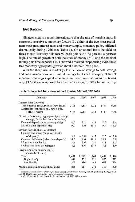
Nineteen sixty-six taught investigators that the rate of housing starts is extremely sensitive to monetary factors. By either of the two most promi- nent measures, interest rates and money supply, monetary policy stiffened dramatically during 1966 (see Table 1). On an annual basis the yield on three-month Treasury bills rose 93 basis points to 4.88 percent, a postwar high. The rate of growth of both the stock of money (M1) and the stock of money plus time deposits (M2) showed a marked drop; during 1966 these two monetary aggregrates grew at about half their 1965 pace.

With the sharp rise in market yields the flow of savings to both savings and loan associations and mutual savings banks fell abruptly. The net increase of savings capital at savings and loan associations in 1966 was only $3.6 billion as opposed to a 1961-65 average of $9.7 billion, a drop

Table 1. Selected Indicators of the Housing Market, 1965-69

Inldicator 1965 1966 1967 1968 1969

Jnterest rates (percent) Three-month Treasury bills (new issues) 3.95 4.88 4.32 5.34 6.68 Mortgages (conventional, new home,

FHLBB series) 5.74 6.14 6.33 6.83 7.66

Growth of monetary aggregates (percentage change, December from December)

Demand deposits plus currency (Ml) 4.7 2.2 6.6 7.2 2.4 Ml plus time deposits (M2) 9.7 4.9 11.1 9.4 -1.5

Savings flows (billions of dollars) Commercial banks (large certificates

of deposit)a 3.8 -0.8 4.7 2.5 -12.0 Commercial banks (other time deposits) 16.2 14.0 19.1 18.1 0.8 Mutual savings banks 3.6 2.6 5.1 4.1 2.5 Savings and loan associations 8.5 3.6 10.7 7.3 4.0

Private nonfarm housing starts (thousands of units)

Total 1,451 1,142 1,268 1,484 1,446 Single-family 941 755 821 875 792 Multifamily 509 386 448 608 654

Mobile home shipments (thousands) 216 217 240 318 390

Sources: Federal Reserve Bulletini, various issues; Conistruction Review, Vol. 16 (February 1970), pp. 25 and 28. Details may not add to totals because of rounding.

a. Certificates of deposit issued in denominations of $100,000 or more.

50 Craig Swan

of 63 percent. The net increase of savings deposits at mutual savings banks also slowed in 1966, although not as dramatically.

Savings and loan associations and mutual savings banks have been major participants in the mortgage market, traditionally allocating increases in deposits to mortgages. From 1955 to 1965 savings deposits at these two institutions increased by $102.5 billion, and mortgage holdings by $108.2 billion. That net increase in home mortgages was two-thirds of the national increment. These observations indicate that changes in deposit inflows to savings and loan associations and mutual savings banks will have a large impact on the availability of mortgage credit. Specifically, substantial declines in inflows will lead to a comparable curtailment of mortgage credit and the rate of housing starts.

During 1966 housing starts took their sharpest drop since the start of the Korean war. The decline was more than 21 percent from 1,450,000 units in 1965 to 1,140,000 units in 1966. From the fourth quarter of 1965 to the fourth quarter of 1966, starts fell more than 42 percent, from an annual rate of 1,549,000 to 897,000. Starts in the fourth quarter of 1966 were at the lowest level of the postwar period. The decline in the annual total of starts from 1965 to 1966 was felt in all types of new residential building, but was somewhat greater for multifamily units (24 percent) than for single-family units (20 percent).

A Simple Model of Housing Starts

The 1966 experience implies a large payoff to models of housing starts that pay particular attention to monetary variables and that structure their use of them to coincide with what is observed in the mortgage market. As shown below, it is possible to explain a large part of the variance of housing starts from 1958 through 1966 by concentrating attention on the flow of funds to savings and loan associations and mutual savings banks.2 Given

2. The demonstration that movements in housing starts over time and in 1966 can be explained by looking at the flow of funds to savings and loan associations and mutual savings banks begs the question of whether other models, with a different focus, can do the same thing. Without pretending to be exhaustive with respect to the treatment of other models, we would note the following: (1) Ex post prediction of 1966 with the residential construction equations of the Wharton model overesti- mate the level and underestimate the decline of private nonfarm residential construction. (2) Recent versions of the Maisel model have been revised to include several monetary variables with close links to the mortgage market.


the importance of mortgage financing to most homebuilding decisions, it is surprising that financial variables reflecting the availability of mortgage credit received so little attention from econometric investigators prior to 1966.

Mortgage market variables are of concern because it is reasonable to presume that monetary factors act on housing activity largely through the mortgage market. Are there alternative formulations of the impact of monetary factors that do as well in explaining housing activity in 1966? Or-put another and currently more relevant way-are changes in the money supply sufficient by themselves to explain the variation in the rate of housing starts over time? While we have not exhausted alternative formulations of such a hypothesis, we conclude that changes in the money supply fail to explain fully the fluctuations of housing starts.

The following model is offered to illustrate the importance of the availability of mortgage credit for housing starts. The rate of nonfarm housing starts is assumed to be a function of the inflow of funds to savings and loan associations and mutual savings banks, the mortgage rate in the previous quarter, and a time trend. The inflow of funds is measured by the average during the previous two quarters of the net increase in deposits at savings and loan associations and mutual savings banks plus the net increase in advances from the Federal Home Loan Banks to savings and loan associations. Also estimated were equations that included the rate of housing starts in the previous quarter.

The flow of funds to mutual savings banks and savings and loan associations is included to reflect major movements in the availability of mortgage credit. For both types of institutions deposit flows and mortgage lending are tightly linked. For savings and loan associations the link is primarily the result of regulation; they have virtually no alternative. For mutual savings banks the link is one of choice since they can acquire other assets, primarily corporate bonds, but have chosen not to do so except in times of relative yield advantage. Evidence on the sluggishness of mortgage rates and the rationing of mortgage credit suggests that mortgage markets are quite often in disequilibrium and that mortgage rates are an insufficient measure of the availability of mortgage credit.

The time trend is included to pick up slowly changing factors such as income, prices, and population. Increased population clearly raises the required number of housing units. With a focus on housing starts, the emphasis is on changes in the number of units, and the relevant population

52 Craig Swan

concept is the change in the number of households. From 1958 to 1966, net household formation varied little from year to year, and thus little information was lost by its omission from the regression. In any case, econometric verification of its importance during this period is difficult.

The levels of income and relative prices probably have more impact on the value of units started than on the number. The effect of income on starts is probably concentrated on their timing; for example, a temporary drop in income postpones the demand for new units. Over the longer run, as incomes rise, people primarily demand better houses, rather than more of them, although demand for second homes is enhanced.

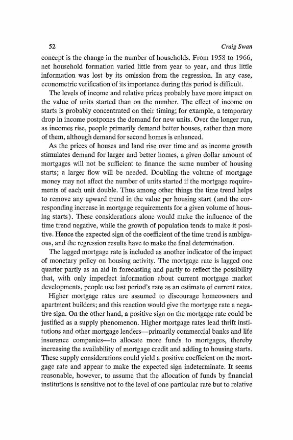
As the prices of houses and land rise over time and as income growth stimulates demand for larger and better homes, a given dollar amount of mortgages will not be sufficient to finance the same number of housing starts; a larger flow will be needed. Doubling the volume of mortgage money may not affect the number of units started if the mortgage requirements of each unit double. Thus among other things the time trend helps to remove any upward trend in the value per housing start (and the corresponding increase in mortgage requirements for a given volume of housing starts). These considerations alone would make the influence of the time trend negative, while the growth of population tends to make it positive. Hence the expected sign of the coefficient of the time trend is ambigu- ous, and the regression results have to make the final determination.

The lagged mortgage rate is included as another indicator of the impact of monetary policy on housing activity. The mortgage rate is lagged one quarter partly as an aid in forecasting and partly to reflect the possibility that, with only imperfect information about current mortgage market developments, people use last period's rate as an estimate of current rates.

Higher mortgage rates are assumed to discourage homeowners and apartment builders; and this reaction would give the mortgage rate a negative sign. On the other hand, a positive sign on the mortgage rate could be justified as a supply phenomenon. Higher mortgage rates lead thrift institutions and other mortgage lenders-primarily commercial banks and life insurance companies-to allocate more funds to mortgages, thereby increasing the availability of mortgage credit and adding to housing starts. These supply considerations could yield a positive coefficient on the mortgage rate and appear to make the expected sign indeterminate. It seems reasonable, however, to assume that the allocation of funds by financial institutions is sensitive not to the level of one particular rate but to relative


rates of return. When associated with high returns on alternative assets, high mortgage rates need not produce more funds for mortgages. As postwar experience indicates, higher mortgage rates usually are accompanied by a smaller relative yield advantage for mortgages.

Regression results are presented below. In order to minimize the sensitivity of the results to the inclusion of 1966, the equations have been estimated to exclude data for that year. They were estimated for 1958: 1 to 1965:4.

(1) HS = 3012.2 - 6.5T + 39.7AG - 328.5Rm_ (1.5) (3.0) (3.2)

R2 = 0.66, standard error = 85.2.

(2) HS = 2148.1 - 3.6T + 18.2AG - 267.6Rm1l + 0.5HS1 (1. 1) (1.6) (3.3) (4.5)

R2 = 0.80, standard error = 65.8.

where HS = private nonfarm housing starts, in thousands, seasonally adjusted

annual rate Rm = average interest rates for conventional mortgages on both new

and existing houses (FHA series) T = quarterly time trend with T = 1 (for 1958:1)

AG = 0.5 E (AD + AS + AF), t-1

in which AD = net change in deposits of mutual savings banks, seasonally

adjusted annual rate in billions of dollars AS = net change in savings capital at savings and loan associations,

seasonally adjusted annual rate in billions of dollars AF = net change in Federal Home Loan Bank advances to savings

and loan associations, seasonally adjusted annual rate in billions of dollars.

Numbers in parentheses are t statistics.

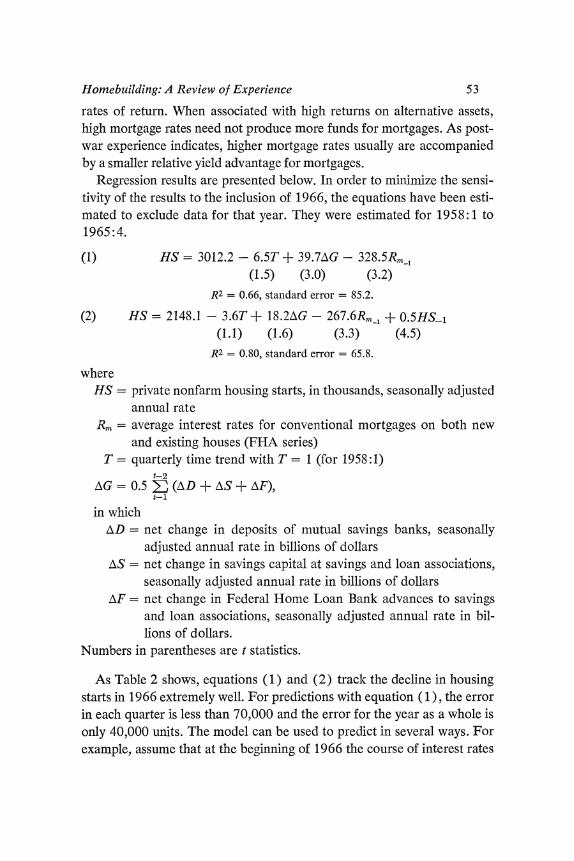
As Table 2 shows, equations (1) and (2) track the decline in housing starts in 1966 extremely well. For predictions with equation (1), the error in each quarter is less than 70,000 and the error for the year as a whole is only 40,000 units. The model can be used to predict in several ways. For example, assume that at the beginning of 1966 the course of interest rates

54 Craig Swan

Table 2. Comparison of Actual Private Nonfarm Housing Starts with Predictions Based on Regression Equations, by Quarter, 1966 and 1969

Thousands of units, seasonally adjusted annual rate

Predictions Year and Actual quarter starts Eqluation (1) Equation (2)

1966 1 1,395 1,327 1,392 2 1,250 1,241 1,293 3 1,056 1,039 1,121 4 897 830 908

Year 1,149 1,109 1,178

1969 1 1,692 1),510a 1,559a 2 1,496 1a558a 1a548a 3 1,414 1,460a 1,470a 4 1,299 1,214a 1X275a

Year 1,475 1,435a 1,463a

Sources: Actual, Econzomic Report of the Presiden2t, February 1968 and Febriuary 1970; predictions, estimated from regression equations (1) and (2) discussed in text.

a. Intercept adjusted for error in predicting fourth quarter of 1968.

and savings flows can be foreseen with perfect accuracy, what are the implications for housing activity during the year? Equation (2), which has lagged housing starts, can be used "recursively"; that is, the estimate of housing starts for the first quarter can be used in estimating housing starts in the second quarter, the estimate for the second quarter in estimating for the third, and so on. As Table 2 shows, recursive predictions with equation (2) track housing starts in 1966 quite closely. The error for the year is only 29,000 units.

Both equations mark the sharp downturn in 1966 astonishingly well. From the first to the fourth quarter, equations ( 1 ) and (2) show a drop in housing starts of 497,000 and 484,000 units, respectively. The actual decline was 498,000 units. The time trend accounts for a small loss of 20,000 units. The increase in the mortgage rate and the sharp drop in the inflow of funds contribute equally to the rest of the decline.

In a period with no dramatic shift in the rate of household formation, income, or prices, the availability and cost of mortgage credit can domi- nate the behavior of housing starts. The first three factors establish the level around which activity varies in the short run with changes in the availability of mortgage credit. During the early sixties the long-run deter-


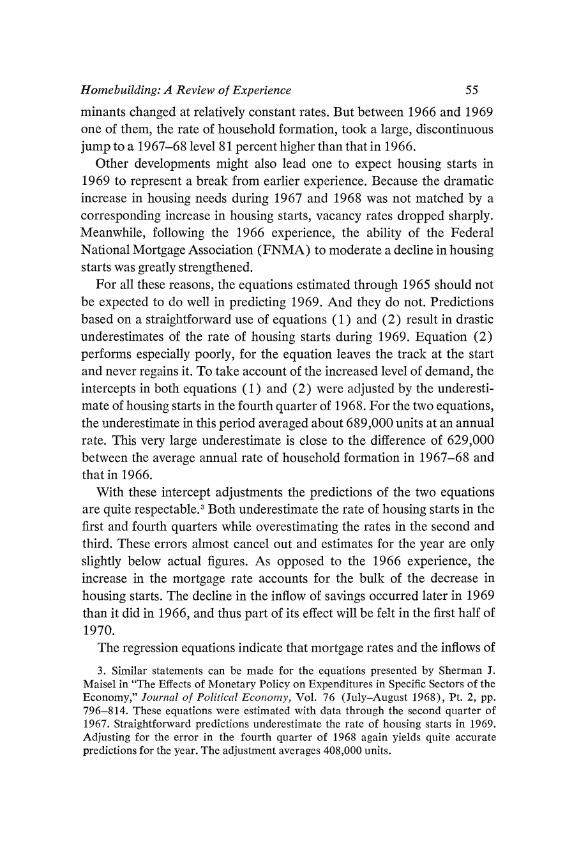
minants changed at relatively constant rates. But between 1966 and 1969 one of them, the rate of household formation, took a large, discontinuous jump to a 1967-68 level 81 percent higher than that in 1966.

Other developments might also lead one to expect housing starts in 1969 to represent a break from earlier expelience. Because the dramatic increase in housing needs during 1967 and 1968 was not matched by a corresponding increase in housing starts, vacancy rates dropped sharply. Meanwhile, following the 1966 experience, the ability of the Federal National Mortgage Association (FNMA) to moderate a decline in housing starts was greatly strengthened.

For all these reasons, the equations estimated through 1965 should not be expected to do well in predicting 1969. And they do not. Predictions based on a straightforward use of equations (1) and (2) result in drastic underestimates of the rate of housing starts during 1969. Equation (2) performs especially poorly, for the equation leaves the track at the start and never regains it. To take account of the increased level of demand, the intercepts in both equations (1) and (2) were adjusted by the underestimate of housing starts in the fourth quarter of 1968. For the two equations, the underestimate in this period averaged about 689,000 units at an annual rate. This very large underestimate is close to the difference of 629,000 between the average annual rate of household formation in 1967-68 and that in 1966.

With these intercept adjustments the predictions of the two equations are quite respectable.3 Both underestimate the rate of housing starts in the first and fourth quarters while overestimating the rates in the second and third. These errors almost cancel out and estimates for the year are only slightly below actual figures. As opposed to the 1966 experience, the increase in the mortgage rate accounts for the bulk of the decrease in housing starts. The decline in the inflow of savings occurred later in 1969 than it did in 1966, and thus part of its effect will be felt in the first half of 1970.

The regression equations indicate that mortgage rates and the inflows of

3. Similar statements can be made for the equations presented by Sherman J. Maisel in "The Effects of Monetary Policy on Expenditures in Specific Sectors of the Economy," Journal of Political Econiomy, Vol. 76 (July-August 1968), Pt. 2, pp. 796-814. These equations were estimated with data through the second quarter of 1967. Straightforward predictions underestimate the rate of housing starts in 1969. Adjusting for the error in the fourth quarter of 1968 again yields quite accurate predictions for the year. The adjustment averages 408,000 units.

56 Craig Swan

funds to savings institutions explain housing starts satisfactorily in 1958- 66. But they also demonstrate that to explain fully the level of starts in 1969 one must also look at the basic demand factors-income, prices, and population. The next section discusses the events of 1969 with an emphasis on these points.

1969 Revisited

Even without the credit crunch of 1966, one might reasonably have been bealish about housing in that year, if one had judged the prospects by vacancy rates.4 The same measure of the demand for housing could have foretold the strength of homebuilding in 1969.

Vacancy rates at the end of 1965 were quite high by postwar standards: The rate for rental units (the number of vacant rental units as a proportion of total rental units) was 7.7 percent for the country as a whole. It ranged from 5.1 percent in the Northeast to 11.7 percent in the West. The rate for all units, rental and homeowner, ranged from 2.5 percent in the Northeast to 5.7 percent in the West. As evidenced by vacancy rates, tremendous overbuilding had taken place in the West. Starts there were at high levels in the early sixties, peaked in 1963, and then dropped rapidly. However, vacancy rates kept rising through 1965. By the end of 1968 things had changed considerably. Nationally the vacancy rate of rental and homeowner units had dropped almost one-third to 2.3 percent; in the West it dropped sharply to 3.1 percent.

POPULATION, INCOME, AND PRICES

As indicated above, the last few years have seen a surge in the rate of household formation. From 1960 through 1966 the annual average was 870,000, and in 1966 formations were about 100,000 below this average. During the next two years, 2,808,000 households were formed for an average of 1,404,000 a year, over 61 percent higher than the 1960-66 average. Census projections, which underestimated the 1967 and 1968 experience, show a continuation of high rates of household formation

4. Certain basic definitions link household formation, starts, and vacancies. For example, the change in vacancies is given by the difference between housing starts and the sum of removals and household formation. Thus an examination of vacancy rates is an alternative to looking at household formation relative to starts.


throughout the next decade. During 1967 and 1968 combined, new housing starts, public and private, farm and nonfarm, totaled 2,870,000. Subtracting the increase in households, each of which by definition occu- pies one housing unit, from the number of units started leaves only 62,000 units for replacement of old units and increases in second homes. But these last two factors have been estimated to claim 700,000 to 800,000 units a year.

Where did the housing units come from to meet the high levels of demand? One source, as mentioned before, was a reduction in the number of vacant units. Another source was mobile homes. Shipments of 217,000 mobile homes in 1966 were virtually unchanged from the previous year. But shipments increased by 10.5 percent in 1967, by 32 percent in 1968, and by 23 percent in 1969, to 390,000 units. Not all mobile homes are used for living quarters.5 Some serve as offices and some as school dormi- tories, which are excluded from the housing stock. One estimate of these alternative uses, which is needed to determine the contribution of mobile home production to the housing stock, assigns half of the production of mobile homes in 1966 to them. On the assumption that since 1966 these alternative uses have continued to grow at the rate of overall production in earlier years, the contribution of mobile home production to the housing stock was 250,000 units in 1969, compared with 108,000 units in 1966. This contribution has risen from about 9 percent of housing starts in 1966 to over 17 percent in 1969. Mobile homes have been an especially important source of low-cost housing; they are estimated to constitute 90 percent of all recently built housing valued at less than $15,000.

Measures of the number of new units and new households take little account of the traditional determinants of demand-income and prices. Both the income and price elasticities of the demand for housing are subject to considerable uncertainty. Estimates of both run from 0 to 2.0. Striking a balance in the middle, let us tentatively pick 1.0 for both elasticities. From 1965 through 1968, the nonfarm housing stock, measured in constant dollars, increased by 5.6 perent. This figure comes from cumu- lating past expenditures on residential construction with an allowance for depreciation at the rate of 2.5 percent per year. The figures make no allow-

5. Data on mobile homes have not been systematically integrated with other data on homebuilding. For example, in the national income accounts, outlays on mobile homes are lumped with the automobile component rather than with residential construction.

58 Craig Swan

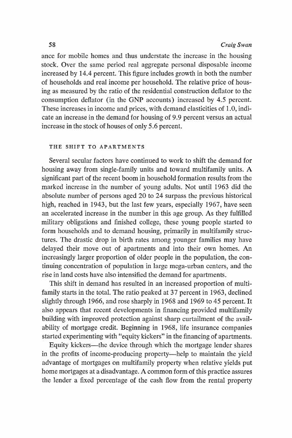
ance for mobile homes and thus understate the increase in the housing stock. Over the same period real aggregate personal disposable income increased by 14.4 percent. This figure includes growth in both the number of households and real income per household. The relative price of housing as measured by the ratio of the residential construction deflator to the consumption deflator (in the GNP accounts) increased by 4.5 percent. These increases in income and prices, with demand elasticities of 1.0, indicate an increase in the demand for housing of 9.9 percent versus an actual increase in the stock of houses of only 5.6 percent.

THE SHIFT TO APARTMENTS

Several secular factors have continued to work to shift the demand for housing away from single-family units and toward multifamily units. A significant part of the recent boom in household formation results from the marked increase in the number of young adults. Not until 1963 did the absolute number of persons aged 20 to 24 surpass the previous historical high, reached in 1943, but the last few years, especially 1967, have seen an accelerated increase in the number in this age group. As they fulfilled military obligations and finished college, these young people started to form households and to demand housing, primarily in multifamily struc- tures. The drastic drop in birth rates among younger families may have delayed their move out of apartments and into their own homes. An increasingly larger proportion of older people in the population, the continuing concentration of population in large mega-urban centers, and the rise in land costs have also intensified the demand for apartments.

This shift in demand has resulted in an increased proportion of multifamily starts in the total. The ratio peaked at 37 percent in 1963, declined slightly through 1966, and rose sharply in 1968 and 1969 to 45 percent. It also appears that recent developments in financing provided multifamily building with improved protection against sharp curtailment of the availability of mortgage credit. Beginning in 1968, life insurance companies started experimenting with "equity kickers" in the financing of apartments.

Equity kickers-the device through which the mortgage lender shares in the profits of income-producing property-help to maintain the yield advantage of mortgages on multifamily property when relative yields put home mortgages at a disadvantage. A common form of this practice assures the lender a fixed percentage of the cash flow from the rental property


above some agreed-upon level, in addition to interest payments on the principal of the loan.

Informal observation indicates that in 1969 life insurance companies made extensive use of equity kickers, although how much cannot be deter- mined from available data. Their continued strong accumulation of multifamily mortgages is one indicator of the importance of this financing tech- nique. From 1968 to 1969, although net acquisitions of total mortgages by life insurance companies dropped by $300 million, net acquisitions of multifamily mortgages rose by $200 million. Between 1965 and 1969 the rate of acquisition of home mortgages by life insurance companies changed by $2 billion from a net increase of $1.1 billion in 1965 to a net decrease of $0.9 billion in 1969. At the same time acquisitions of multifamily mortgages dropped only $0.4 billion from $1.6 billion to $1.2 billion.

The development of equity kickers may be part of the explanation for the improved performance of multifamily as opposed to single-family starts in 1969. It may also be partially responsible for the underestimate of starts in the first quarter even after the intercept adjustment. On an annual basis multifamily starts rose in 1969 by 46,000 units while single- family starts fell by 83,000 units. Multifamily starts were quite strong in the first half of 1969, especially in the first quarter when the adjusted equations (1) and (2) underestimated the rate of total housing starts. By the end of 1969, however, multifamily starts had fallen almost as much as single-family starts. Even so, this contrasted with 1966, when the percentage decrease in multifamily starts was greater than that for single-family starts.

Any discussion of recent developments in the American economy must take account of inflation and recognize the possible role of inflationary expectations. One reason suggested for the drop in housing starts in 1966 is that prospective homeowners were slow to build expectations of inflation into their demand for houses and were priced out of the market as mortgage rates rose. By 1969 prospective homeowners had adjusted their expectations in line with recent experience. Thus in spite of nominal mortgage rates of 8 percent and higher, the expectation of continued inflation has dampened the increase in real mortgage rates anticipated by homebuyers.

In summary, by the beginning of 1969 there was not only strong basic demand for housing but also little unused inventory to meet it. At the same

60 Craig Swan

time, demand was shifting toward multifamily units, which were better able to resist a tightening of mortgage credit.

INFLOWS TO SAVINGS INSTITUTIONS

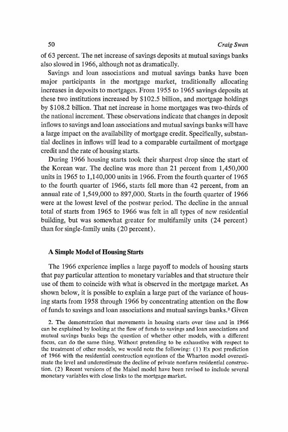
In 1969, as in 1966, both mutual savings banks and savings and loan associations experienced a massive slowdown in the net inflow of savings. As Figure 1 iliustrates, savings flows have been quite sensitive to the movement of market interest rates. During 1966 savings flows dried up as market rates rose rapidly and the rates offered depositors could not be raised to match. From September 1966 to January 1970 rates on passbook savings were held essentially constant under new regulatory authority granted in 1966. In late 1966 and early 1967 the flow of deposits picked up from earlier low levels, reflecting a continued decline in market rates. As this trend in rates was reversed in late 1967 and 1968, deposit flows receded from their 1967 levels. Then in 1969, with the dramatic increase

Figure 1. Savings Flows at Savings Institutions and the Rate on Three- month Treasury Bils, by Quarter, 1965-69

Billions of dollars Percent (seasonially adjuisted annual rate) 20 8

Treasuiry bill rate / (right scaile) ,

15 6

10 ------ / 4

Savings flowvsa 2 (left scale)

I I I I I I 0

1965 1966 1967 1968 1969

Source: Federal Reserve Bulletini, various issues. a. Net increase in savings deposits at mutual savings banks plus net increase in savings capital at

savings and loan associations.


in market rates, savings flows again plummeted, dropping even lower than they had in 1966.

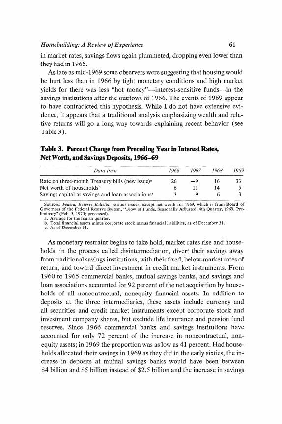
As late as mid- 1969 some observers were suggesting that housing would be hurt less than in 1966 by tight monetary conditions and high market yields for there was less "hot money"-interest-sensitive funds-in the savings institutions after the outflows of 1966. The events of 1969 appear to have contradicted this hypothesis. While I do not have extensive evidence, it appears that a traditionial analysis emphasizing wealth and relative returns will go a long way towards explaining recent behavior (see Table 3).

Table 3. Percent Change from Preceding Year in Interest Rates, Net Worth, and Savings Deposits, 1966-69

Data itemn 1966 1967 1968 1969

Rate on three-month Treasury bills (new issue)a 26 -9 16 33 Net worth of lhouseholdsb 6 11 14 5 Savings capital at savings and loan associations, 3 9 6 3

Sources: Federal Reserve Biilletini, various issues, except net worth for 1969, which is from Board of Governors of the Federal Reserve System, "Flow of Funds, Seasonally Adjusted, 4th Quarter, 1969, Pre- liminary" (Feb. 5, 1970; processed).

a. Average for the fourth quarter. b. Total financial assets minus corporate stock minus financial liabilities, as of December 31. c. As of December 31.

As monetary restraint begins to take hold, market rates lise and households, in the process called disintermediation, divert their savings away from traditional savings institutions, with their fixed, below-market rates of return, and toward direct investment in credit market instruments. From 1960 to 1965 commercial banks, mutual savings banks, and savings and loan associations accounted for 92 percent of the net acquisition by households of all noncontractual, nonequity financial assets. In addition to deposits at the three intermediaries, these assets include currency and all securities and credit market instruments except corporate stock and investment company shares, but exclude life insurance and pension fund reserves. Since 1966 commercial banks and savings institutions have accounted for only 72 percent of the increase in noncontractual, nonequity assets; in 1969 the proportion was as low as 41 percent. Had households allocated their savings in 1969 as they did in the early sixties, the increase in deposits at mutual savings banks would have been between $4 billion and $5 billion instead of $2.5 billion and the increase in savings

62 Craig Swan

capital at savings and loan associations would have been $14 biflion instead of $4 billion.

During 1969 mortgage lending by savings and loan associations was maintained at very high levels in the face of what by the end of the year became a complete collapse of savings flows. Continued mortgage lending was made possible in part by vigorous support from the Federal Home Loan Banks. Advances to savings and loan associations increased by $4 billion in 1969, resulting in a 77 percent increase in advances outstanding by the end of 1969. By contrast the net increase in advances in 1966 was only $938 million; although advances had increased by $1,345 million through July, repayments exceeded advances for the rest of the year, as savings flows picked up.

The 1966 experience seems peculiar. One would think that savings and loan associations would have wanted to borrow at such a time and that the authorities would have been willing to increase advances to stem the decline in housing starts.

By April 1966 the Federal Home Loan Banks had virtually exhausted their ability to make further advances without additional borrowing of their own, and this was inhibited by federal government budget considerations and concern over the adverse effects on market interest rates. In late April the Federal Home Loan Bank Board announced a tightening in the policy on advances. Savings and loan associations were instructed to gear their mortgage lending to their actual cash flow, with predictable results for housing starts. According to the equations cited above, each $1 billion of lost advances cost 35,000 to 40,000 housing starts. By contrast in 1969 the Federal Home Loan Banks were able to respond vigorously to the plight of the savings and loan associations. Freed of federal budgetary considerations, borrowing by the Federal Home Loan Banks increased by $3.7 billion in 1969 and advances increased by $4 billion, as opposed to increased borrowing of only $1.6 billion and increased advances of only $0.9 billion in 1966. The $4 billion in advances in 1969 was responsible for 140,000 to 160,000 starts.

The limited ability of the Federal Home Loan Banks to meet the demand for advances in 1966 was reflected in the dramatic drop in mortgage commitments by savings and loan associations. From March 1966, when they peaked, to December 1966, outstanding commitments slid more than 50 percent from $3.3 billion to $1.5 billion. During 1969, as associations


were able to borrow from the Federal Home Loan Banks while adjusting to a lower rate of increase in savings shares, the drop in commitments, as measured by either the percentage or absolute decline, was less severe. The reduction of commitments also appears to have been smoother in 1969 than in 1966.

FNMA was another source of substantial support for the mortgage market in 1969. During 1966 the association, like the Federal Home Loan Banks, was constrained in its actions by inclusion in the federal budget. In that year FNMA raised only $1,916 million and acquired only $1,810 million in mortgages. Its transfer to private ownership in 1968 allowed FNMA to be much more aggressive in its response to the decline in starts in 1969. During 1969 it raised $4,135 million and acquired $3,669 million in mortgages. As a source of funds for home mortgages, FNMA moved from a position of virtually no importance in the early sixties to one second only to that of the savings and loan associations in 1969. From 1960 to 1965 its mortgage holdings were approximately unchanged. In 1966 the association supplied 17 percent of the net increase in home mortgages. In 1969 the figure was 24 percent and by the fourth quarter it was 44 percent.

During the fourth quarter of 1968 net acquisitions of home mortgages by FNMA were at an annual rate of $1.1 billion. During the fourth quarter of 1969, they had risen to a rate of $6.2 billion. Equations (1) and (2) take no explicit account of the tremendous increase in the association's activity, and yet they track the decline in housing starts in 1969 quite well. From the fourth quarter of 1968 to the fourth quarter of 1969, increased residential mortgage acquisitions by FNMA were almost exactly balanced by reduced acquisitions by lenders other than the thrift institutions. Thus these factors not explicitly considered by the regression equation appear to have offset each other. This same offsetting occurred in 1966. If increased FNMA activity does not simply offset decreased activity by other lenders, forecasts of housing activity should be modified accordingly. As a first approximation, FNMA acquisitions could be weighted equally with increased savings flows since the two result in similar increases in mortgage acquisitions. This procedure implies that in 1969 the association was responsible for 140,000 to 160,000 housing starts.

There is a problem in distinguishing between the gross and the net impact on housing starts of increased activity by FNMA and the Federal Home Loan Banks. The measures we have derived are measures of the

64 Crai2 Swan

gross impact. They assume that everything else is unchanged-in particular, savings flows and interest rates. Increased activity by FNMA and the Federal Home Loan Banks entails increased borrowings, which, in turn, boost market interest rates and accentuate any deposit drain from thrift institutions. Since these federal credit agencies started borrowing on a large scale, households have consistently taken large amounts of their obligations. In 1966 households absorbed over 80 percent of the net increase in the liabilities of federal credit agencies; in 1969 they added $4.5 billion of credit agency securities to their portfolios. Recent increases in the minimum size of FNMA and Treasury obligations may lessen their attractive- ness to individuals, forcing them back to the intermediaries, but they also raise some serious questions of equity.

What would have happened to savings flows in 1969 if net borrowing by FNMA and the Federal Home Loan Banks had been zero instead of $7.7 billion? To answer this question with precision would require detailed knowledge of the portfolio decisions of households. But some rough calcu- lations may be suggestive. Assume that households would have rechan- neled the $4.5 billion in funds used to purchase credit agency securities entirely into time deposits at commercial banks and savings deposits at the thrift institutions. Assume further that the distribution between banks and thrift institutions would have followed the average pattern of recent inflows. Then deposits at thrift institutions would have been $1.8 billion higher. Presumably these funds would still have found their way into mortgages. With no net borrowings by FNMA and the Federal Home Loan Banks, the gross flow of funds to the mortgage market would have been reduced by $7.7 billion. But the net contribution by FNMA and the Fed- eral Home Loan Banks should be placed $1.8 billion lower-or $5.9 billion-by this calculation. The net impact is thus estimated as 77 percent of the gross impact.

PORTFOLIO ADJUSTMENTS IN 1969

High levels of deposit inflows in early 1969 were accompanied by a buildup in liquid assets of savings and loan associations. Given their more liquid position and a lowering of the liquidity requirement in June, savings and loan associations were able during late 1969 to draw down their holdings of cash and government securities and maintain mortgage lending at a rate higher than the increase in savings capital and advances from the Fed-


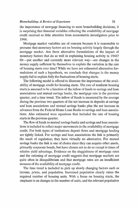
eral Home Loan Banks (Table 4). Preliminary data show net mortgage acquisitions during the fourth quarter of 1969 at an annual rate of $8.0 billion, although the net increase in savings capital and advances was at an annual rate of only $3.2 billion. To finance the high level of lending, associations were selling government securities at an annual rate of $5.7 billion. For the year as a whole the reduction in cash and government securities was $1.36 billion, nearly matching the $1.5 billion by which mortgage

Table 4. Net Change in Selected Balance Sheet Items of Savings Institutions, 1968 Annual and 1969 by Quarter

Billions of dollars, seasonally adjusted annual rate

1969 Type of inistitittion and

balance sheet item 1968 1 2 3 4a

Savings and loan associations Savings shares 7.3 8.8 5.6 3.2 -1.5 Advances 0.9 3.1 2.7 5.6 4.7 Mortgages 9.3 10.3 10.7 9.1 8.0 Government securities 0.6 3.5 3.4 1.0 -5.7

Mutual savings banks Deposits 4.1 4.1 2.8 1.2 1.9 Mortgages 2.8 2.9 2.7 2.1 1.9 Government securities -0.3 0.1 -0.1 -1.2 -0.7 Corporate bonds 1.4 0.8 0.8 -0.3 0.4

Commercial banks Large certificates of depositb 2.5 -16.7 -15.4 -12.3 -3.5 Other time deposits 18.1 7.6 5.1 -9.3 -0.2 Mortgages 6.7 8.0 5.9 3.2 2.6

Source: Board of Governors of the Federal Reserve System, "Flow of Funds, Seasonally Adjusted, 4th Quarter, 1969."

a. Preliminary. b. Certificates of deposit issued in denominations of $100,000 or more.

acquisitions exceeded deposit flows and advances. The reduction in the liquidity requirement from 6.5 percent to 6 percent freed almost $700 million of liquid assets. It is interesting to note that, with the dramatic increase in interest rates since 1965, the proportion of cash in the liquidity holdings of savings and loan associations has been substantially reduced. At the end of 1965 cash holdings were 34 percent of liquid assets; in 1969 they were only 22 percent.

In 1969 net mortgage lending by mutual savings banks was $2.4 billion,

66 Craig Swan

virtually matching net deposit inflows of $2.5 billion. This emphasis on mortgage lending was more in line with earlier experience and in contrast with the experience of 1967 and 1968, when mutual savings banks accu- mulated substantial amounts of corporate bonds. Following the increase in the interest rate ceiling on insured mortgages in January 1969, the yield spread between corporate bonds and insured mortgages, which form the largest portion of mutual savings bank mortgage holdings, moved in favor of mortgages for most of the year. Also there are indications that mutual savings banks use corporate bonds to adjust portfolios: New funds are ini- tially held as corporate bonds and later reallocated to mortgages. As deposit inflows slow down, the accumulation of corporate bonds also tends to slow down.

Mortgage acquisitions by commercial banks were surprisingly strong in 1969. From 1967 to 1968 they rose almost 50 percent. In 1969 the rate dropped, but only to the levels of 1966 and 1967. This continued acquisition during 1969 is all the more surprising in view of the tremendous loss of time deposits. In 1968 they had increased by $20.6 billion; in 1969 they decreased by $11.2 billion, a swing of more than $30 billion. It should be noted that the acquisition of mortgages slowed appreciably during the year.

In summary, how was 1969 different from 1966? A major difference was the higher level of basic demand in 1969. Recent growth in the number of households, along with previously depressed levels of housing starts, produced in the first quarter of 1969 the highest level of housing starts since 1955. The trend toward multifamily dwellings that accompanied the development of the potential for equity participation by the lender helped part of the housing market to defend itself as mortgage credit became tighter. Even with some adjustment for its competitive effect vis-'a-vis the savings institutions, aggressive action on the part of the Federal Home Loan Banks and FNMA helped both to ease the transition to a lower level of savings flows and to increase the supply of residential mortgage money.

How were 1966 and 1969 the same? Events during 1969 again demon- strated the sensitivity of investment in housing to monetary factors, in particular to the availability of mortgage credit. In spite of surprising strength throughout the year, housing starts declined more than in any other four quarters during the postwar period except 1966 and 1950-51. The social significance of the decline was especially great in view of the recent high rate of household formation.


Prospects for 1970 and Beyond

As long as the availability of mortgage credit is closely linked to specialized financial intermediaries (in 1969 savings and loan associations and mutual savings banks still supplied 60 percent of home mortgages), large changes in the flow of funds to these institutions will be mirrored in major swings in housing activity. If a higher and more stable level of housing starts is desirable social policy, dramatic shifts in monetary conditions must be avoided and new sources of financing must be developed. If the level of homebuilding nevertheless remains lower than socially desirable, the federal government will have to undertake explicit support of the housing or mortgage market.

The problem of disintermediation arises when market rates rise precipi- tously-when monetary policy bears too large a share of the burden of restraining demand-and when the specialized financial institutions, owing either to the nature of their assets and liabilities or to official regulation, cannot maintain their competitive position in the struggle for household savings. The solution to the problem involves a better balance of policy between monetary and fiscal restraint and an improvement in the competitive ability of the specialized financial institutions. If this means a deemphasis of their role as mortgage lenders, so be it. Such a move would require development of new sources of financing for homebuilding on its present scale. With or without any deemphasis of mortgage lending by the savings institutions, these new sources of financing must be forthcoming if the levels of homebuilding projected for the seventies are to be met.

What do the regression results indicate for housing starts in the early seventies? The projection discussed below makes use of equation (1) with the 1969 intercept adjustment. Retaining the adjustment is a reasonable first approximation because projected rates of household formation for the early seventies are quite similar to the actual rates of 1967 and 1968. These results also assume that mortgage rates decline to and remain at 7 percent, that the allocation of savings by households returns to the pattern of the early sixties, that noncontractual, nonequity assets of households grow at their 1960-69 trend, and that the stock of advances from the Federal Home Loan Banks is held constant.

With these assumptions equation (1) (adjusted) implies an average of 2,050,000 starts a year for the period 1971-75. The 1969 President's

68 Craig Swan

Report on National Housing Goals calls for an annual average of 2.3 million starts over the same period. To meet this goal would require an additional $4 billion a year of increased savings flows or FNMA activity. In the President's 1970 Housing Report, the targets for homebuilding have been scaled down, allowing for the contribution of mobile homes to the national goals. Even so, more than 2.5 million starts are called for in 1975 while the adjusted equation predicts only 2.1 million.

Several points should be kept in mind when considering these projections. No allowance is made for any broadening of the investment oppor- tunities for the savings institutions that would break the tight link between deposit flows and mortgage lending. If learning by doing is a pervasive phenomenon, it may be difficult to reestablish earlier savings patterns. Both these factors would lead to an even more pessimistic forecast.

On the other hand, these projections do not allow for expanded opera- tions for FNMA to direct funds into mortgages. Although it is called by a different name, FNMA acts like the savings institutions in some respects. It borrows short to lend long and its holdings are concentrated overwhelm- ingly in one long-term asset, mortgages. If interest rates are relatively stable or fall, this is not a risky venture. However, when rates rise rapidly, FNMA, like the savings institutions, can get into serious trouble as the cost of its liabilities rises more rapidly than the revenue from its assets.

Still another consideration not taken into account in the projections is a return of vacancy rates to more normal levels. Such a development would further increase the demand for housing, tending to elicit additional funds, but also contributing to the strong pressures on credit supplies.

A promising means to expand the sources of mortgage financing is the development of a mortgage-backed security. The interest and principal of the security can come from a specific pool of mortgages insured by the Federal Housing Administration or guaranteed by the Veterans Adminis- tration, with additional guarantees by the Government National Mortgage Association (GNMA). If a mortgagor should default, GNMA would han- dle the liquidation while maintaining payments to the holder of the security. To a prospective investor these securities offer competitive yields backed by a government guarantee, but without the paper work and cost of making the same investment in mortgages directly. The security is expected to be especially attractive to pension and retirement funds, which to date have held very small amounts of mortgages. At the end of 1968 these funds had assets of $144.1 billion and mortgage holdings of only $9.3 billion, about


6 percent of total assets. By contrast they held $50.9 billion in corporate bonds, about 35 percent of total assets.

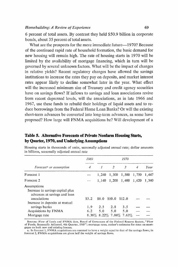
What are the prospects for the more immediate future-1970? Because of the continued rapid rate of household formation, the basic demand for new housing will remain high. The rate of housing starts in 1970 will be limited by the availability of mortgage financing, which in turn will be governed by several unknown factors. What will be the impact of changes in relative yields? Recent regulatory changes have allowed the savings institutions to increase the rates they pay on deposits, and market interest rates appear likely to decline somewhat later in the year. What effect will the increased minimum size of Treasury and credit agency securities have on savings flows? If inflows to savings and loan associations revive from recent depressed levels, will the associations, as in late 1966 and 1967, use these funds to rebuild their holdings of liquid assets and to re- duce borrowings from the Federal Home Loan Banks? Or will the existing short-term advances be converted into long-term advances, as some have proposed? How large will FNMA acquisitions be? Will development of a

Table 5. Alternative Forecasts of Private Nonfarm Housing Starts, by Quarter, 1970, and Underlying Assumptions Housing starts in thousands of units, seasonally adjusted annual rate; dollar amounts in billions, seasonally adjusted anntual rate

1969 1970

Forecasta or assuimption 4 1 2 3 4 Year

Forecast 1 - 1,240 1,300 1,500 1,750 1,447

Forecast 2 - 1,140 1,200 1,400 1,620 1,340

Assumptions Increase in savings capital plus

advances at savings and loan associations $3.2 $8.0 $10.0 $12.0 - -

Increase in deposits at mutual savings banks 1.9 2.5 2.8 3.5

Acquisitions by FNMA 6.2 5.0 5.0 5.0 Mortgage rate 8.36% 8.22%/0 7.86%60/ 7.63%0 -

Sources: Flow of fuindis and FNMA data, Board of Governors of the Federal Reserve System, "Flow of Funds, Seasonally Adjusted, 4th Quarter, 1969"; mortgage rates, author's estimates for rates on mortgages on both new and existing houses.

a. In forecast 1, FNMA acquisitions are assumed to have a weight equal to that of the savings flows; in forecast 2, FNMA acquisitions are given half the weight of savings flows.

70 Craig Swan

mrortgage-backed security progress fast enough during the year for it to be a significant influence?

Two forecasts for 1970 are shown in Table 5. Both assume that savings flows to the thrift institutions will rise sharply, because of higher rates offered there, decreased market yields, and the recent increases in the minimum denomination of federal government and credit agency securities. By the third quarter of 1970 savings flows are assumed to be at levels reached in early 1969. In line with standard forecasts, with recent experience of reduced growth in GNP, and with a shift to an easier stance of monetary policy, both forecasts assume that mortgage rates will decline by the end of 1970 to their level of early 1969. The assumption underlying the forecasts is that mortgage rates will follow the same path down in 1970 that they followed up in 1969. The difference between the two forecasts comes from different weights given to FNMA acquisitions. Forecast 1 weights them equally with savings flows while forecast 2 assigns them half the weight of savings flows. Striking a balance between the two forecasts suggests that private nonfarm housing starts in 1970 will be at a rate of 1,400,000 units.

Comments and

Discussion

Sherman Maisel: I would like to focus on the problems of using econometric models for homebuilding.

One problem is the question of whether variables that logically belong in the model should be included even though you could do as well or better, statistically, without them. In this case, the underlying theory says that household formation or vacancies or something of that sort ought to be included. These variables were not important during the period to which the equations were fitted, but they became important during the period of projection. Therefore, they have to be invoked to explain the discrepancy between the projection and the model.

This is a problem that we all face. The answer depends on the purpose of the model. For forecasting purposes, you may want a model that con- tains the variables that could be important during the forecast period, even though it does not fit history quite so well as others.

The second point is that federal policy changes account for a structural change in the equations between 1966 and 1969. As a result of 1966, it was generally recognized that the Federal Home Loan Bank Board had not really stood up to the market in the way it should have, and that the pro- cedures of the Federal National Mortgage Association were inadequate. As a result of this experience, the way the Home Loan Bank Board han- dled its own liquidity and also the liquidity in the associations was changed rather drastically. This increased the ability of the Home Loan Banks to meet the 1969 experience, which shows up in the model as one of the

71

72 Craig Swan

important factors in 1969. An equivalent change took place in FNMA, when it dropped the rationing process that had been set up in 1966 and instead went to the new auctioll procedure.

During the last half of 1969, more than half the money going into the mortgage market came through FNMA and the Home Loan Banks. There was a tremendous shift in the form of intermediation-away from deposit institutions and toward federal credit agencies. But this aid to home- builders does not help model builders. The policy makers learn as a result of experience, but when they do learn, they create problems for the model based on the previous period, since it could not reflect the structural change brought about by the policy change. I think this is emphasized very well in Swan's paper.

Having made these adjustments in the 1969 explalnation, you must be extremely cautious in using the old model for a 1970 projection or a 1975 projection. The change in household formation obviously remains important. The low current vacancy rates also have to be recognized. The financial variables that were so important in the 1969 situation, as was brought out in Swan's paper, can be expected to remain important in the future.

William Branson: As I read it, Craig Swan's paper has two major parts. First, he presents a single equation for housing starts, based on 1958-65 data, that predicts the 1966 collapse fairly well. But that equation greatly underpredicts housing starts in 1967-69. The second main part of the paper is a discussion of why starts were so much higher in 1969 than was predicted by the initial equation. Essentially, Swan suggests in the latter discussion that there has been a large upward shift in the demand for housing, due mainly to the surge in household formation since 1967 and evidenced by the sharp drop in vacancy rates. With this shift in demand, out- put of housing has been limited by supply of funds.

The equations mix supply and demand considerations. The mortgage interest rate is related negatively to the level of starts in the 1958-65 equation. This suggests that higher rates discouraged homebuyers more than they encouraged lenders; the demand effect was dominant. On the other hand, the flow of funds to the mutual savings banks and to savings and loan associations is included, with a positive sign. This variable reflects supply.

What apparently happened after 1966 was a big upward shift in demand, which is documented in the second half of the paper. This shift in


demand must have been a contributing factor to the higher level of interest rates on mortgages. Thus when the equation for 1958-65 is used to estimate 1969, no account is taken of the shift in demand. It should not be surprising that the estimates are terrifically low.

My point is that if Swan's equations were analyzed more closely from the point of view of supply and demand in the housing market, they would fit in better with the discussion of the 1969 housing situation.

Finally, there is not so big a discrepancy between the projections of housing starts to 1975 and the new targets set forth in the Council of Eco- nomic Advisers' Annual Report for 1970. Swan's 2.1 million projection compares with a target of 2.4 million-after deducting for mobile homes. That is not a striking difference. However, attaining the housing projections depends on the right aggregate federal budget policy. A substantial federal surplus is required to achieve the level of starts in the Council's Annual Report and in the President's Report on Housing.

Craig Swan: I did not make a further adjustment in the level of the initial equation for predicting the period 1971-75, since the expected rate of household formation is very much in line with what we had in 1967 and 1968. This would indicate that a first approximation could be obtained by leaving the adjustment factor alone rather than pulling something out of the air.

There is the question Branson raised of whether periods of high interest rates on mortgages should be viewed as encouraging, greater supplies of funds. I would argue that the supply of funds may depend upon the relative yield of mortgages compared with other securities-rather than the absolute yield. It appears from postwar experience that high absolute mortgage rates are, in fact, associated with a reduced yield advantage for mortgages. That would seem to indicate that the availability of mortgage credit would fall even further in periods of generally high interest rates.

General Discussion

Several participants raised various problems of forecasting in an area where the structure of the market has changed so much over the past several years. It was stressed that, in projecting the 1971-75 period, Swan's adjusted equations must be used with particular care and healthy skepti-

74 Crai, Swan

cism. The author had emphasized the shift in the basic structure of demand and supply in the housing market between 1966 and 1969. While the rate of household formation seemed likely to hold reasonably steady for the next several years, other factors could not be assumed to return to a pas- sive state. Among the factors that could alter the structure further in the future are changes in the relative strength of demands for mobile homes and conventional single-family dwellings; changes in buyers' expectations about inflation in construction; and financial innovations, either publicly or privately generated.

Various issues about the past and prospective growth of the mobile home industry were raised by Daniel Brill, Alan Greenspan, and John Kareken. Since mobile homes have been financed through installment loans of high yield, supplies of funds to this area have not fallen off sharply during periods of tight money. Consequently, part of the strength of mobile home production could be the temporary result of the particular squeeze of tight credit markets on home mortgages. Alan Greenspan stressed the importance of knowing whether mobile homes are primarily substitutive for housing starts or for net or gross conversions of existing housing, or whether they are reflected in changes in the rate of demolitions and in vacancies. R. J. Cord-on pointed out that the especially rapid rate of inflation in residential building probably also contributed to the demand for mobile hom-es (as well as for rental apartments) by pricing some peo- plI out of the singyle-family market. The need for better data and analysis of these issues was stressed buLt no one claimed to have answers.

It was noted that both in the past and in the years ahead changes in price expectations could significantly affect demands of homebuyers. If homebuyers expect rapid inflation in the prices of single-family dwellings, they are less deterred by higher interest rates on mortgages. William Fellner pointed out that the real rate of interest on mortgages-the nominal rate adjusted for expected price increases-might actually be lower in 1969 than in 1966, especially in view of the particularly rapid inflation in the homebuilding area. R. J. Gordon expanded on this thesis and hypothe- sized that the real rate of interest has probably fallen more for housing than for investment in plant and equipment because of the differential rates of inflation in the two sectors.

Saul Hymans questioned this analogy, however, stressing that homes were purchased to yield a flow of services that are consumed rather than marketed. Sherman Maisel noted the importance of distinguishing between


factors that affect the level of housing starts and those that affect the dollar value per new home. He suggested that price considerations-both relative and absolute, both current and expected-are likely to have more significant effects on how much house people feel they can afford than on decisions to stay single, double up, or otherwise fail to form a household.

The structure of lhome financing was explored. Robert A. Gordon cau- tioned against "an almost exclusive emplhasis on the mutual saviings baLnks and the savings and loan associations. In the first ten or fifteen years of the postwar period, differences between mortgage interest rates and yields on securities seemed to have an important influence on the way financial institutions like insurance companies and commercial banks movled back and forth between mortgages and marketable securities." He argued that the behavior of this important fringe of mortgage lenders could lbecome significant once again.

R. J. Gordon mentioned regulatory ceilings on comlmercial banks and on thrift institutions as a determinant of the flow of savings to the various types of financial intermediaries. He argued that the differei tial of rates paid by savings and loans over rates on commercial bank timie deposits is unlikely to return to the high level of the early 1960s. Hence savings and loans are unlikely to reestablish the very large share of household savings that they obtained in the earlier period. In that event, Swan's housing projections might prove to be too optimistic.

William Poole wondered whether the discussion of housing credit over- emphasized imperfections on the supply side. As the author had pointed out, differentials between mortgage yields and comparable market yields, such as on Aaa bonds, tend to narrow during periods of tight money. During 1969, the differential between mortgage yields and Aaa bond yields had narrowed even more than in 1966. Poole suggested that one would normally look at demand rather than supply to explain such a development. If demand for mortgages had been that strong, why had it not pulled mortgage rates up relative to other yields? David Fand expanded on this puzzle, noting that a high interest elasticity of demand by homebuyers would account for mortgage yields lagging behind other yields in a period of tight money. Indeed, if demand is really as intense and inelastic as is sometimes suggested, one would expect a much greater flow of funds into mortgages from commercial banks and other intermediaries that do not specialize in mortgage lending.

Maisel felt, however, that the curious behavior of the yield differentials

76 Craig Swan

could probably be accounted for best by the fact that the primary mortgage lenders are "local institutions subject to local pressure and local regula- tions and local legislation" that may keep them channeling funds into mortgages and make them relatively unresponsive to changes in yields on alternative assets. In particular, when the usury ceilings of many states held mortgage rates down, local mortgage lenders were under pressure to continue supplying funds at the ceiling rate. It was also noted that reported mortgage interest rates may have important statistical biases during periods of tight money, failing to reflect some improved returns to the lender stem- ming from "points," tighter terms on the mortgage, and other devices. The possible role of continuing relationships between the institutions and their customers was also cited.

Robert A. Gordon pointed to the capital stock adjustment process as the most convenient framework for analyzing homebuilding. This approach requires a focus, first, on the determinants of the desired capital stock and, second, on the adjustment process that closes the gap between the desired and existing stock. Household formation is obviously relevant to determining the desired capital stock. Demolitions, conversions, mobile homes, and the like all fit neatly into this framework. Monetary factors could be important in determining, both the desired capital stock and the short-run rate at which the existing stock adjusts to the desired level. Maisel pointed out, however, that traditional capital stock adjustment models have not worked well in the housing area. He concluded: "I am convirnced you have to explain it as an inventory model in which the relevant inventory is that of vacant units and the key factor is the willingness of builders or apartment developers to add to that inventory. Unlike other areas of inventory investigation, it is clear in this area that the entrepreneur is sensitive to interest rates and to the availability of funds in his decisions on how much inventory to carry."

homebuilding: a review of experience - brookings · homebuilding: a review of experience 49 1966...

Documents