holistic mass balance modeling approach for chemical ... · pdf fileholistic mass balance...

1

Holistic Mass Balance Modeling Approach for Chemical Screening and Priority Setting

Jon ArnotNSERC Postdoctoral Fellow

University of Toronto [email protected]

EPA Exposure Science Community of Practice (ExpoCoP)July 14, 2009

2

Overview of presentation

• Rationale / background• Risk Assessment, IDentification And Ranking (RAIDAR)

– Screen and prioritize organic chemicals with greatest exposure, hazard and risk potential to humans and the environment

– Illustrate key concepts of RAIDAR model– Illustrative applications for risk priority setting of ~1,100 Canadian

Domestic Substances List (DSL) chemicals

• Holistic vs. current “PBT” screening methods• Model comparisons with monitoring data (PBDE 99)• Addressing uncertainty• Farfield Human Exposure (FHX) model• Questions

3

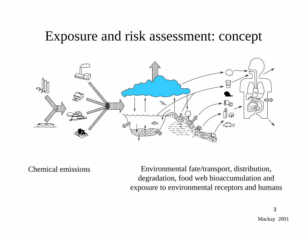
Environmental fate/transport, distribution, degradation, food web bioaccumulation and

exposure to environmental receptors and humans

Chemical emissions

Exposure and risk assessment: concept

Mackay 2001

4

Rationale: chemical assessments

• Regulatory programs require the assessment of a large number of chemicals (~100,000), e.g., UN Stockholm Convention, Canadian Environmental Protection Act 1999, TSCA, REACH

• Methods and criteria developed in 70s and 80s now being applied to screen and prioritize chemical lists

• Typical current approach is PBT “bright line” categorization

• Enormous task with little measured data available, limited resources and it is not practical to measure “everything” ($$, animal testing, people power)

5

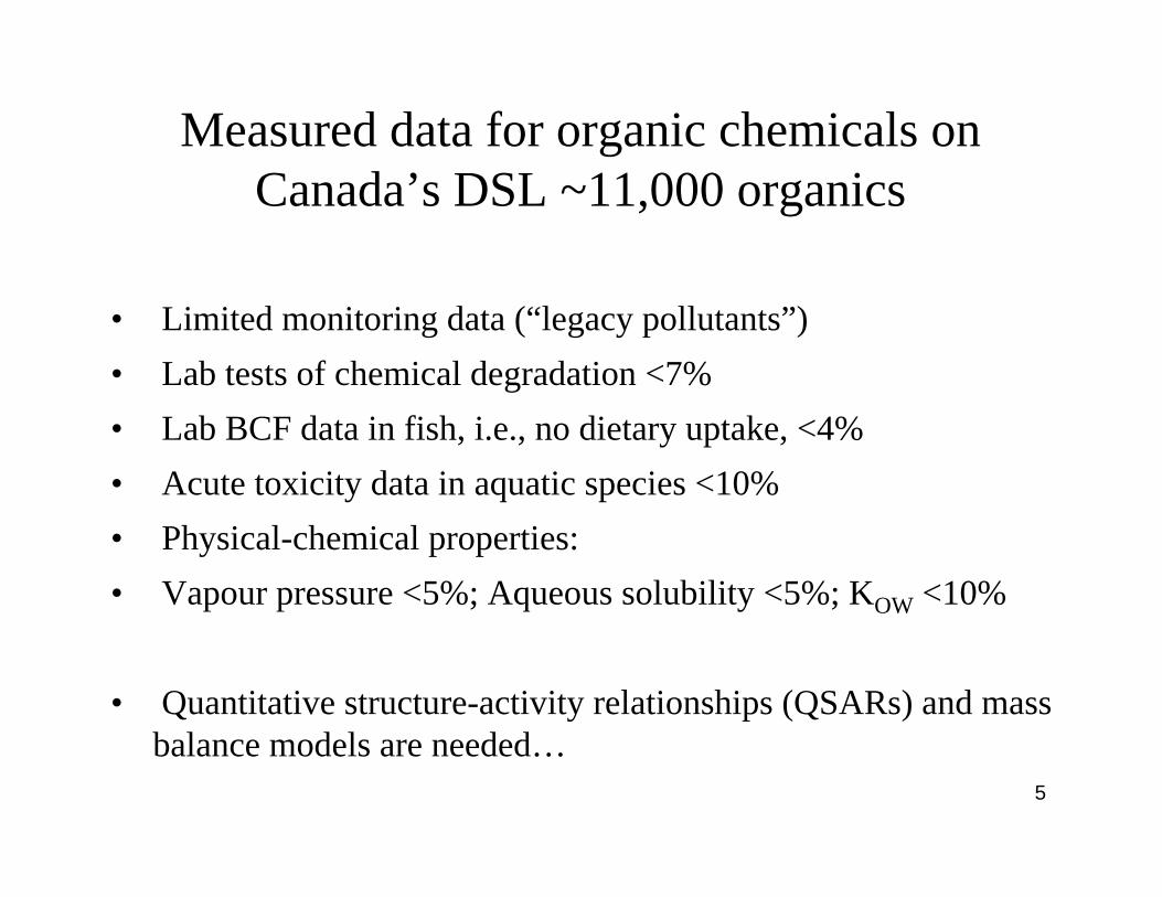
• Limited monitoring data (“legacy pollutants”)• Lab tests of chemical degradation <7% • Lab BCF data in fish, i.e., no dietary uptake, <4%• Acute toxicity data in aquatic species <10%• Physical-chemical properties:• Vapour pressure <5%; Aqueous solubility <5%; KOW <10%

• Quantitative structure-activity relationships (QSARs) and mass balance models are needed…

Measured data for organic chemicals on Canada’s DSL ~11,000 organics

6

General objectives

• Develop a mass balance modelling framework for estimating exposure and risk potential to identify and rank organic chemicals for more comprehensive assessments (monitoring and modelling)

• Bring together available information on chemical partitioning, degradation, fate and transport, food web bioaccumulation, exposure and effect in a transparent and “holistic” model

• Save uncertain actual emissions information for the last step inthe exposure and risk calculations

7

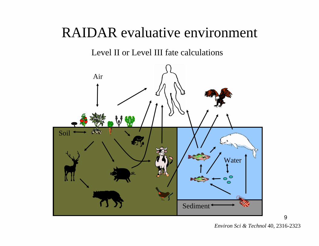
RAIDAR evaluative model

1. Physical component (Air, Water, Soil, Sediment)– Regional scale environment, i.e., 105 km2

– Level II or III fate calculations (“box” models)

2. Biological component– “Representative” ecological and human receptors, flexible selection of biological properties– Mechanistic mass balance food web bioaccumulation models

• Aquatic, terrestrial, agricultural species• Chemical specific biomagnification and biotransformation

Multimedia mass balance exposure and risk assessment model~ EUSES, CalTOX, but different; notably the treatment of

food web bioaccumulation (Birak et al. 2001)

8

RAIDAR exposure, hazard and risk metrics

• RAF – Risk Assessment Factor

• HAF – Hazard Assessment Factor

• EAF – Exposure Assessment Factor

• BAF – Bioaccumulation Factor

• iF – intake fraction, intake rates

• TBB – Total Body Burdens, internal dose

• POV – Overall Persistence

9

Air

Sediment

Soil

Water

RAIDAR evaluative environmentLevel II or Level III fate calculations

Environ Sci & Technol 40, 2316-2323

10

Vegetation models

Foliage vegetation

0

2

4

6

8

10

12

14

2 4 6 8 10 12 14 16

log KOA

log

(CFV

/ C

GA)

DDs_DFs

CBs_PCBsPAHs

Root vegetation

-6

-4

-2

0

2

0 2 4 6 8 10log KOW

log

(BC

F ro

ot k

g.kg

-1 w

w)

CBs_UK_carrotsPAHs_UK_potatoesPAHs_UK_carrotsPAHs_Greece_carrotsHCHs_DDX_China_various


11

Diet

Water

Metabolic transformation

Growth ‘dilution’

Fecal egestion

Diet

Water


Growth ‘dilution’

Fecal egestion

Water ventilating organisms (KOW)

Empirical biomagnification factors – capture biomagnification potential

Absorption, Metabolism, Elimination – assumed a “well mixed compartment”

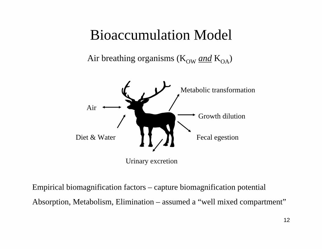
Bioaccumulation Model

12

Air

Diet & Water


Growth dilution

Urinary excretion

Fecal egestion

Bioaccumulation Model

Empirical biomagnification factors – capture biomagnification potential

Absorption, Metabolism, Elimination – assumed a “well mixed compartment”

Air breathing organisms (KOW and KOA)

13

Running the model

• Input requirements:– Physical-chemical properties: KOW, SW, VP, pKa– Half-lives: biodegradation, biotransformation, hydrolysis,

oxidation, photolysis– Consistent Toxicity or Threshold endpoint for risk ranking –

CT (e.g. critical body residue)

• Unit emission rate – EU (kg/h)– Arbitrary value, “seeds” the model (e.g. 1 kg/h)– Circumvents initial need for actual emission rate – EA (kg/h)

14

e.g., pyrene fate and distribution calculations

1 kg /h

5020 kg

2.79E-04 g/m3

674 kg

6.74E-10 g/m3

2.40E-07 g/m3

6.51E-04 g/m3

48.0 kg

3260 kg

9.97E-05 μPa

8.25E-03 μPa

1.00E-03 μPa

2.91E-03 μPa

3.41E-05

1.49E-04

4.80E-04

0.674

0.275

0.003950.0345

0.0206

0.0196

0.00651

0.00410

0.02050.007140.0178

1 kg /h

5020 kg

2.79E-04 g/m3

674 kg

6.74E-10 g/m3

2.40E-07 g/m3

6.51E-04 g/m3

48.0 kg

3260 kg

9.97E-05 μPa

8.25E-03 μPa

1.00E-03 μPa

2.91E-03 μPa

3.41E-05

1.49E-04

4.80E-04

0.674

0.275

0.003950.0345

0.0206

0.0196

0.00651

0.00410

0.02050.007140.0178

1 kg /h

5020 kg

2.79E-04 g/m3

674 kg

6.74E-10 g/m3

2.40E-07 g/m3

6.51E-04 g/m3

48.0 kg

3260 kg

9.97E-05 μPa

8.25E-03 μPa

1.00E-03 μPa

2.91E-03 μPa

3.41E-05

1.49E-04

4.80E-04

0.674

0.275

0.003950.0345

0.0206

0.0196

0.00651

0.00410

0.02050.007140.0178

15

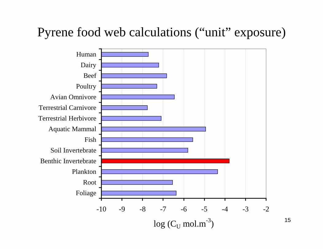
Pyrene food web calculations (“unit” exposure)

-10 -9 -8 -7 -6 -5 -4 -3 -2

FoliageRoot

PlanktonBenthic Invertebrate

Soil InvertebrateFish

Aquatic MammalTerrestrial HerbivoreTerrestrial Carnivore

Avian OmnivorePoultry

BeefDairy

Human

log (CU mol.m-3)

16

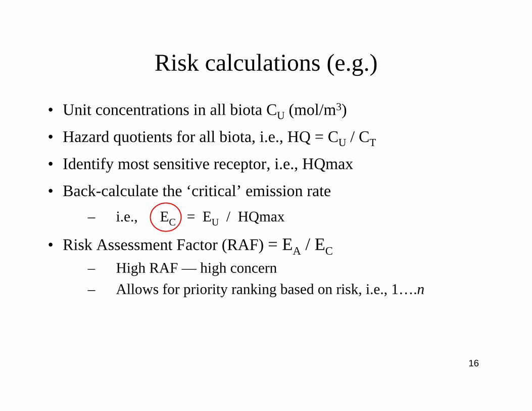
Risk calculations (e.g.)

• Unit concentrations in all biota CU (mol/m3)

• Hazard quotients for all biota, i.e., HQ = CU / CT

• Identify most sensitive receptor, i.e., HQmax

• Back-calculate the ‘critical’ emission rate– i.e., EC = EU / HQmax

• Risk Assessment Factor (RAF) = EA / EC – High RAF — high concern– Allows for priority ranking based on risk, i.e., 1….n

17

-20

-15

-10

-5

0

5

10

-5 0 5 10log KOW

log

KA

W

Prioritizing risk: a case study

• 1,100 Canadian DSL organic chemicals

• EU = 1 kg/h• EA DSL quantity estimates

• Selected effect endpoint– CT

– DSL acute lethality data– Critical body residues

18

-16-14-12-10

-8-6-4-2024

0 100 200 300 400 500 600 700 800 900 1000 1100

Chemical ID #

log

RA

F L_

II

A

B

C

D

E

F

G

Prioritizing risk: n = 1,100

19

0.17052357728140309G0.3819457308456439450F0.29719313457256365251E0.11439811978219379D0.032041764196215C0.0038221061B0.0001800100A

Average frequencyCountCountCountCountCountRIB

n = 1,100LIII Soil

LIII Water

LIIIAir

LIII A,W,SLII

Prioritizing risk

20

Screening and priority setting methods

Current POP and PBT screening and “priority setting”methods (ca. 1970s-1980s):1. Hazard assessment: multiple categories (PBT), “bright

line cutoff” criteria, e.g., “B” or “not B”; screened “in”or “out”

2. Risk assessment: (exposure/effects, uncertainty) for those chemicals screened “in”

Binary scoring in multiple categories makes it difficult to assign priorities: “is a P&T worse than a B&T ?”

21

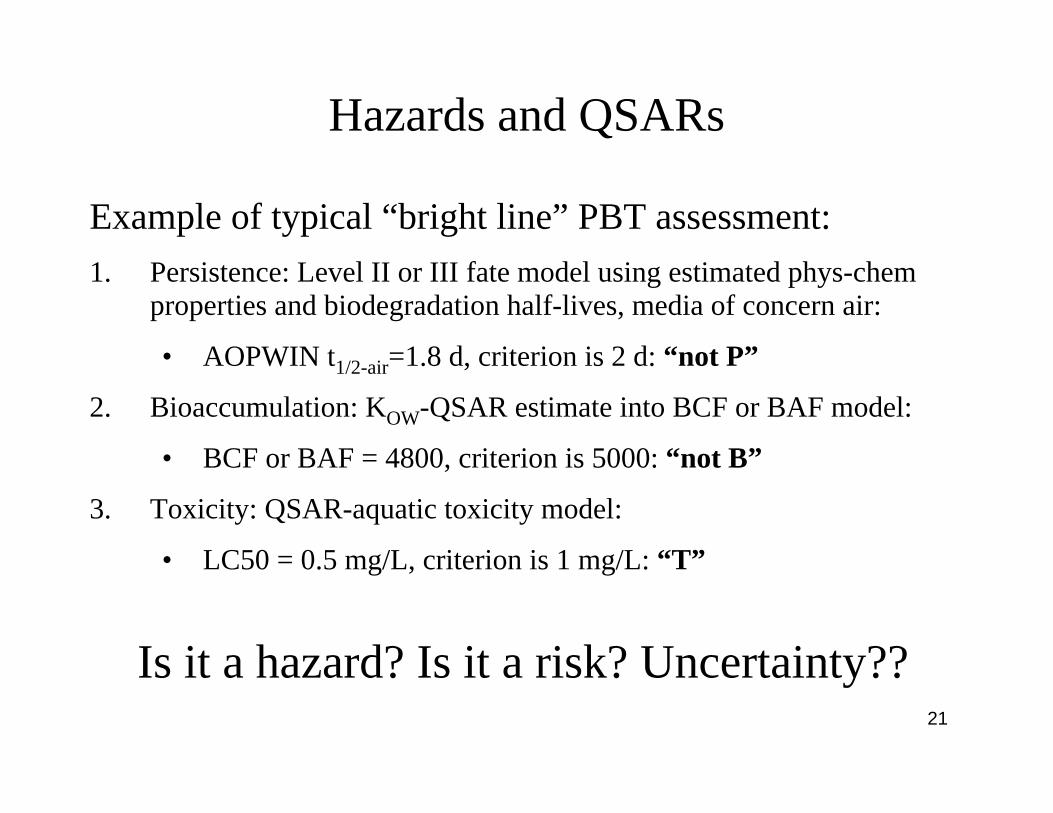
Hazards and QSARs

Example of typical “bright line” PBT assessment:1. Persistence: Level II or III fate model using estimated phys-chem

properties and biodegradation half-lives, media of concern air:

• AOPWIN t1/2-air=1.8 d, criterion is 2 d: “not P”

2. Bioaccumulation: KOW-QSAR estimate into BCF or BAF model:

• BCF or BAF = 4800, criterion is 5000: “not B”

3. Toxicity: QSAR-aquatic toxicity model:

• LC50 = 0.5 mg/L, criterion is 1 mg/L: “T”

Is it a hazard? Is it a risk? Uncertainty??

22

Canada is the first to conduct PBT assessments on existing chemicals

Canadian DSL ~23,000 chemicals (~11,000 organics)

Health CanadaHealth Canada Environment CanadaEnvironment Canada

Domestic Substances ListDomestic Substances List

Health CanadaHealth Canada Environment CanadaEnvironment Canada

Greatest Potential for Human Exposure

Greatest Potential for Human Exposure

Persistent or BioaccumulativePersistent or

Bioaccumulative

P or BInherently Toxic to

Humans


Humans


Non-Human Organisms


Non-Human Organisms

Screening-Level Risk AssessmentScreening-Level Risk Assessment

Meet criteria DSL “in” or DSL(I)

~4,000 “further attention”

Doesn’t meet criteria DSL “out” or DSL(O)

~19,000 “no further action”

Risk assessments are projected until 2025 and beyond

23

Risk is essentially a function of 3 major components:

1. Chemical emission to the environment (Q or EA; mol/h)

2. Exposure or “delivery” (P&B, D; h/m3)

3. Threshold level (toxicity) (T; m3/mol or 1/CT)

“Holistic” risk calculation

Risk Assessment Factor:

RAF = EADT = exposure/effect (uncertainty)

24

1. Risk Assessment Factor (RAF) ƒ(Q,P,B,T)

2. Hazard Assessment Factor (HAF) ƒ(P,B,T)

3. Exposure Assessment Factor (EAF) ƒ(P,B)

Holistic hazard and risk calculationsCombine elements of exposure, hazard and risk in a coherent mass

balance modelling framework for holistic screening methods

Calculate single values for transparent chemical comparisons forranking and priority setting based on exposure potential, “combined

hazard” or risk objectives

25

Policy Analysis: current vs holistic methods Current methods: Canadian DSL categorization; chemicals screened “in” or “out” based on PBT values and bright line cut-off criteria

Holistic methods: RAIDAR EAF, HAF and RAF calculations

Chemicals selected for a case study:

• 100 DSL chemicals “in” – DSL(I), “further attention”

• 100 DSL chemicals “out” – DSL(O), “no further action”

• 12 Stockholm Convention POPs (benchmark)

1. Use same basic information available for the categorization for RAIDAR calculations, i.e., “no biotransformation”

2. Include estimates for biotransformation using novel QSAR

26

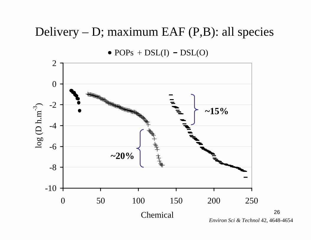
Delivery – D; maximum EAF (P,B): all species

-10

-8

-6

-4

-2

0

2

0 50 100 150 200 250

Chemical

log

(D h

.m-3

)POPs DSL(I) DSL(O)

~20%

~15%


27

Hazard (P,B,T)

-12

-10

-8

-6

-4

-2

0

2

4

0 50 100 150 200 250

Chemical

log

HA

F

HAF_POPs HAF_DSL(I) HAF_DSL(O)


28

-12

-10

-8

-6

-4

-2

0

2

4

0 50 100 150 200 250

Chemical

log

HA

F

HAF_POPs HAF_DSL(I) HAF_DSL(O)

Hazard (P,B,T)

~75% overlap


29

-12

-10

-8

-6

-4

-2

0

2

4

0 50 100 150 200 250

Chemical

log

HA

F or

log

RA

F

HAF_POPs HAF_DSL(I) HAF_DSL(O) RAF_DSL(I) RAF_DSL(O)

Risk (Q,P,B,T)


30

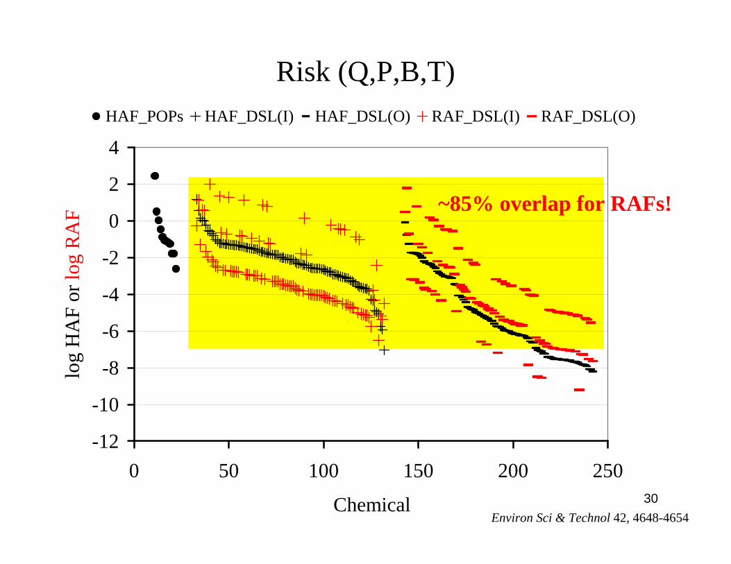
Risk (Q,P,B,T)

-12

-10

-8

-6

-4

-2

0

2

4

0 50 100 150 200 250

Chemical

log

HA

F or

log

RA

F

HAF_POPs HAF_DSL(I) HAF_DSL(O) RAF_DSL(I) RAF_DSL(O)

~85% overlap for RAFs!


31

Predicting biotransformation

• Assuming negligible biotransformation is an “overly conservative” assumption, particularly for chemicals subject to biotransformation

• Biotransformation rate data are needed for hazard and risk assessment to reduce “false positives”

• A QSAR was developed and evaluated to predict primary biotransformation rate constants from chemical structure using in vivo biotransformation rate constant estimates for ~700 chemicals in fish

• U.S. EPA’s EPI Suite Ver. 4.0

Environ Toxicol Chem 28, 1168-1177

32

-16

-14

-12

-10

-8

-6

-4

-2

-16 -14 -12 -10 -8 -6 -4 -2

Level III emissions to water

o: POPs; +: non POPs

Log TBBNo biotransformation assumed

Log

TBB

Bio

trans

form

atio

n in

clud

ed

~108 difference in TBB when estimates included

Human total body burden (TBB) predictions: influence of biotransformation assumptions

Environ Toxicol Chem in press

33

Risk (Q,P,B,T including biotransformation)

-12

-10

-8

-6

-4

-2

0

2

4

0 50 100 150 200 250

Chemical

log

RA

F

RAF_Biotrans_DSL(I) RAF_Biotrans_DSL(O)

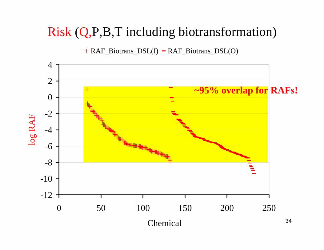
34

~95% overlap for RAFs!

-12

-10

-8

-6

-4

-2

0

2

4

0 50 100 150 200 250

Chemical

log

RA

F

RAF_Biotrans_DSL(I) RAF_Biotrans_DSL(O)

Risk (Q,P,B,T including biotransformation)

35

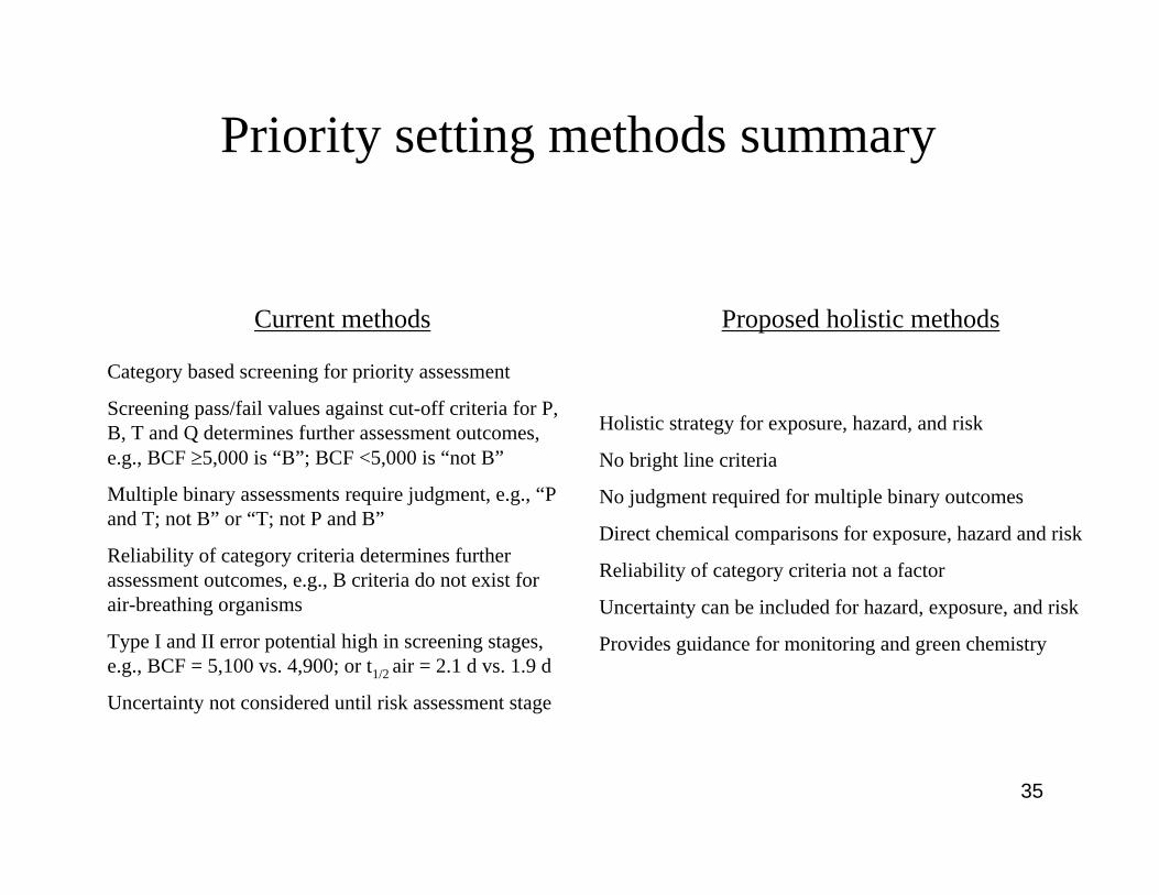
Current methods

Category based screening for priority assessment

Screening pass/fail values against cut-off criteria for P, B, T and Q determines further assessment outcomes, e.g., BCF 5,000 is “B”; BCF <5,000 is “not B”

Multiple binary assessments require judgment, e.g., “P and T; not B” or “T; not P and B”

Reliability of category criteria determines further assessment outcomes, e.g., B criteria do not exist for air-breathing organisms

Type I and II error potential high in screening stages, e.g., BCF = 5,100 vs. 4,900; or t1/2 air = 2.1 d vs. 1.9 d

Uncertainty not considered until risk assessment stage

Holistic strategy for exposure, hazard, and risk

No bright line criteria

No judgment required for multiple binary outcomes

Direct chemical comparisons for exposure, hazard and risk

Reliability of category criteria not a factor

Uncertainty can be included for hazard, exposure, and risk

Provides guidance for monitoring and green chemistry

Proposed holistic methods

Priority setting methods summary

36

Implications

• Based on available information current chemical assessment methods are not effective at setting priorities for risk assessment• Potential for errors using current methods is high meaning limited resources will be “mis-applied” to chemicals of low risk while chemicals with high risk potential may not be evaluated• Complementary holistic methods can enhance current chemical assessment efforts by focusing assessment on chemicals that posethe highest risks (better emissions estimates and toxicity data)• Policies need to adapt as the science evolves (“70s-80s”)

37

RAIDAR evaluation

• Case study for commercial pentabromodiphenyl ether (PBDE-99)• Determine realistic “actual” emission rate estimate (EA) for a

regional scale “source” environment• Exploit linearity of the model to scale “unit emission” predictions

to expected concentrations in the real world using more “realistic”estimates for emissions

• Compile monitoring data for PBDE-99 in various environmental media (air, water, fish, meat products, humans, etc)

• Compare model predictions with monitoring data

• Difficult to “validate” evaluative models, e.g., Monitoring data are limited RAIDAR is not “site specific”, “representative conditions” Spatial and temporal issues (heterogeneity, steady-state)

38

PBDE 99: monitoring data (o) / model (x)

-5 -4 -3 -2 -1 0 1 2 3

log concentration

Air (pg/m3)

Water (pg/L)

Soil (ng/g dwt)

Sediment (ng/g dwt)

Integ Environ Assess Manag on-line June 22, 2009

39

-4 -3 -2 -1 0 1 2 3 4

log concentration (ng/g lwt)

Humans

Piscivorous birds & eggs

Marine mammals

Chickens

Various fish (monitoring)

Shellfish

Starlings

Dairy products

Meat products

PBDE 99: monitoring data (o) / model (x)

Integ Environ Assess Manag on-line June 22, 2009

40

PBDE-99 model and monitoring data

-4

-2

0

2

4

-4 -2 0 2 4log monitoring concentrations

RA

IDA

R lo

g pr

edic

ted

Air, water, soil,sediment

Ecologicalcompartments

Human

1:1 line

41

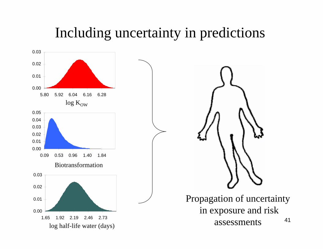
Including uncertainty in predictions

0.00

0.01

0.02

0.03

5.80 5.92 6.04 6.16 6.28

log KOW

0.000.010.020.030.040.05

0.09 0.53 0.96 1.40 1.84

Biotransformation

0.00

0.01

0.02

0.03

1.65 1.92 2.19 2.46 2.73

log half-life water (days)

Propagation of uncertaintyin exposure and risk

assessments

42

• Each of these three “terms” is associated with uncertainty• Actual emissions, i.e., “EA” or “Q”; proportional• 1/CT is indicator of toxic potency, i.e., “T”; proportional• Fate, transport and bioaccumulation, i.e., “D” or CU/EU model state

variables and inputs of phys-chem properties, half-lives (“P&B”)

What dictates uncertainty in the RAF ?

Quantity emittedRAIDAR estimate of

environmental Delivery

RAF = CU 1EU CT

EA

Toxicity of most sensitive receptor

43

Which are the most sensitive and uncertain parameters?What research effort will get the most “bang for the buck”?

Prioritizing uncertainty:

0.00

0.01

0.02

0.03

1.36E-07 6.16E-07 1.10E-06

0.00

0.01

0.02

0.03

5.80 5.92 6.04 6.16 6.28

log KOW

VP (Pa)

0.000.010.020.030.040.05

0.09 0.53 0.96 1.40 1.84

kM fish d-1

0.00

0.01

0.02

0.03

1.65 1.92 2.19 2.46 2.73

log half-life water (days)

45

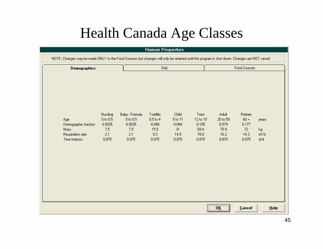
Health Canada Age Classes

46

Health Canada Age Class Specific Intake

47

Some RAIDAR and FHX assumptions• Steady state (not dynamic)• Rate processes follow 1st order kinetics• Results are based on “representative conditions”• “Farfield” exposures to humans

Some limitations• Most discrete organic chemicals (SMILES)• Not recommended for pigments and dyes, and

perfluorinated surfactants, strong acids and bases• Need to improve for chemicals that appreciably dissociate

at environmental and physiological pH

48

Summary• Information on chemical partitioning, fate/transport,

bioaccumulation, exposure and effect endpoint are brought together in a coherent mass balance framework

• Framework is adaptable• RAF rankings span >14 orders of magnitude providing priority

guidance for more comprehensive assessment and monitoring• Fast and affordable for large scale screening using available data,

revisit rankings as better data become available• Uncertainty is inherent whether the data are measured or modelled

and uncertainty can not be totally eliminated • Key parameters can be identified to reduce uncertainty• Assessing risk is the fundamental objective of regulatory programs• Most chemicals can and should be screened for potential risks

49

Some on-going and future research• Indoor exposures to humans• Refined treatment for dissociating substances• Plant uptake models• Absorption efficiency models• Biotransformation rate estimation• Biodegradation rate estimation• Toxicity models• …

Please visit The Canadian Centre for Environmental Modelling andChemistry (CEMC) for a list of publications and model downloads

www.trentu.ca/cemc

50

Acknowledgement

Numerous co-authors on these projects

Environment Canada, Health CanadaNatural Sciences and Engineering Research Council of Canada

(NSERC)Consortium of chemical companies that support our research

(Exxon Mobil Biomedical Sciences)

Thank you for your interest and attention!

holistic mass balance modeling approach for chemical ... · pdf fileholistic mass balance...

Documents