16History Matching of Reservoir Modelsby Ensemble Kalman Filtering: The Stateof the Art and a Sensitivity Study

Leila Heidari, Veronique Gervais, and Mickaele Le RavalecIFP Energies nouvelles, Reservoir Engineering Department, Rueil Malmaison, France

Hans WackernagelGeostatistics Group, Centre de Geosciences, MINES ParisTech, Fontainebleau, France

ABSTRACT

History matching is to integrate dynamic data in the reservoir model–building process. Thesedata, acquired during the production life of a reservoir, can be production data, such as wellpressures, oil production rates or water production rates, or four-dimensional seismic–relateddata. The ensemble Kalman filter (EnKF) is a sequential history-matching method that inte-grates the production data to the reservoir model as soon as they are acquired. Its ease ofimplementation and efficiency has resulted in various applications, such as history matchingof production and seismic data.

We focus on the use of the EnKF for history match of a synthetic reservoir model. First,the method of ensemble Kalman filtering is reviewed. Then the geologic and reservoir char-acteristics of a case study are described. Several experiments are performed to investigate thebenefits and limitations of the EnKF approach in building reservoir models that reproduce theproduction data. Last, special attention is paid to the sensitivity of the method to a set ofparameters, including ensemble size, assimilation time interval, data uncertainty, and choice ofinitial ensemble.

INTRODUCTION

A reservoir model relies on two sources of data: staticdata and dynamic data. Although static data (e.g., geo-logic observations, measurements on cores, logs, etc.)are constant through time, dynamic data change withtime. They include production data measured at wells,such as pressures and oil production rates. As staticdata are too sparse to deterministically describe the spa-

tial variation in transport properties (porosity and per-meability) within the reservoir, they serve to character-ize the parameters of a geostatistical model. Therefore,we refer to a stochastic framework in which reservoirmodels are viewed as realizations of a random function.

Accounting for dynamic data in reservoir modelsis not straightforward, and this process is known as‘‘history matching’’ in the literature. It consists of build-ing a numerical reservoir model, which consists of a

249

Heidari, Leila, Veronique Gervais, Mickaele Le Ravalec, and Hans Wackernagel,

2011, History matching of reservoir models by ensemble Kalman filtering: The

state of the art and a sensitivity study, in Y. Z. Ma and P. R. La Pointe, eds.,

Uncertainty analysis and reservoir modeling: AAPG Memoir 96, p. 249 – 264.

Copyright n2011 by The American Association of Petroleum Geologists.

DOI:10.1306/13301418M963486

grid populated by porosity and permeability valuesthat reproduce the production behavior observed inthe field. Among the various methods proposed for per-forming history matching, the ensemble Kalman filter(EnKF) has recently provided promising results interms of reservoir characterization and uncertaintyquantification. It has beenwidelyused indifferent fields,such as oceanography (Haugen and Evensen, 2002), me-teorology (Evensen and van Leeuwen, 1996), hydrol-ogy (Margulis et al., 2002), and petroleum engineering(Naevdal et al., 2002).

The EnKF is a variation of the well-known KF(Kalman, 1960) for dealing with highly nonlinear prob-lems (Evensen, 1994), as is the case of fluid flow in po-rous media. These filters represent, with error covari-ance matrices, the uncertainties in the reservoir model,with respect to properties such as porosity, permeabil-ity, pressure, saturation, and so on. The model and itsuncertainties are propagated through time accordingto a dynamic system describing fluid flow in porousmedia. Whenever measurements are available, a newestimate for the model and its uncertainties is calculatedby a variance minimization scheme (Evensen, 2007).

Kalman filters are sequential, meaning that the avail-able dynamic data are sequentially integrated in themodeling as soon as they are obtained. Time is dividedinto successive steps or assimilation intervals; eachtime step begins at the end of the previous one andlasts until the next measurements are available. Dur-ing each time step, the filter acts according to two stages.The first stage is forecasting: its purpose is to propagatethe reservoir model by running the flow simulationthrough the time step of interest. The second stage isanalysis (or updating): the reservoir model is updatedby adjusting the numerical flow responses with themeasurements.

In the EnKF, the model uncertainties are representedby an ensemble, that is, a group, of realizations formodel parameters and for model states. Model param-eters are properties such as porosity and permeabilitythat do not change with time, whereas model states areproperties such as pressure and saturations that dochange with time. The mathematical formulation ofthe EnKF (Evensen, 2007) requires the computation ofthe first and second statistical moments, that is, meanand variance for the reservoir parameters and statesthat are derived from an empirical average over a finite-size ensemble of realizations.

Several EnKF applications illustrate the method’smerits and shortcomings that motivated the currentefforts to improve filter performance. The first appli-cation of the EnKF in petroleum engineering was pre-sented by Naevdal et al. (2002) on a two-dimensionalnear-well reservoir model, where permeability mod-

els were predicted. The EnKF proved to provide betterparameter estimations and, consequently, improvedpredictions. Gu and Oliver (2005) applied EnKF tothe three-dimensional PUNQ-S3 model. They foundthe EnKF method more efficient than other history-matching methods in terms of computational burden.In the literature, there exist similar applications of theEnKF on the PUNQ-S3 test case (Lorentzen et al., 2005;Gao et al., 2006). The EnKF was also applied to a facieshistory match by Liu and Oliver (2005), who concludedthat the EnKF was more computationally efficient andeasier to use than gradient-based minimization meth-ods. Real field history matching using the EnKF wasperformed by Haugen et al. (2008) and Evensen et al.(2007), who consider the EnKF to provide a powerfulhistory-matching method. Although the EnKF is gen-erally regarded as a successful method of data assim-ilation, several scientists (Floris et al., 2001; PUNQ-S3test case, 2010) have sought to improve its performance.These improvements concern several assumptions inthe mathematical formulation of the filter that are notsatisfied in practical applications. The four followingparagraphs provide an overview of the main problemsand corresponding proposals.

The EnKF relies on the use of a finite ensemble todescribe the model uncertainties. However, this maylead to spurious correlations in the covariance matrix;unexpected high correlations can be observed for thepoints located far from observation points. In the at-mospheric data assimilation literature (Hamill andWhitaker, 2001; Houtekamer and Mitchell, 2001), adistance-dependent correlation function is used to con-dition the covariance matrix. The idea is to limit theeffect of each observation by considering a cutoff ra-dius beyond which the correlations are negligible.Devegowda et al. (2007) performed a covariance lo-calization based on a streamline-derived function. Itsadvantage is to relate the localization function directlyto the physics of flow in porousmedia. Anderson (2001)discussed the sampling error inherent in the EnKF andsuggested, as a simple remedy, to multiply the covari-ance matrix by a small factor, slightly larger than 1.More sophisticated methods dealing with the prob-lem of spurious correlations can be found in Anderson(2007), Wang et al. (2007), and Fertig et al. (2007).

Another improvement concerns the Gaussian as-sumption for parameters and states in all KFs, includ-ing the EnKF. In reality, nature commonly departs froma Gaussian distribution. For instance, parameters suchas permeability or state variables like water satura-tions commonly do not approximate a Gaussian distri-bution. In addition, even if the initial distributions areGaussian, the nonlinearity of the dynamic model, thatis, the fluid-flow equations, may result in non-Gaussian

250 HEIDARI ET AL.

distributions (Chen et al., 2009). Zafari and Reynolds(2007) applied EnKF to two simple nonlinear problemsto investigate the two problems previously mentionedand concluded that the EnKF provides poor uncer-tainty characteristics when the Gaussian assumptionis violated. Several methods were proposed (Bertinoet al., 2003; Vabø et al., 2008; Moreno et al., 2008) tomodify the EnKF algorithm so that the Gaussianityrequirement is better satisfied.

Next, the use of KFs implies that a linear relation-ship exists between measurements and model param-eters and states, but such an assumption does not holdin fluid flow in porous media (Gu and Oliver, 2007).Wen and Chen (2005) proposed to add a confirmationstep after the updating step in the EnKF algorithm;after each updating step, the fluid-flow simulation isperformed for the current time step with the set ofupdated model parameters so that the dynamic vari-ables are consistent with the model parameters. Zafariand Reynolds (2007) reconsidered the confirmation stepand found it inappropriate within the framework ofthe EnKF. They argued that even for a linear problem,the update of dynamic variables with confirming EnKFmisses some terms obtained by previous time step up-dates. However, Liu and Oliver (2005) suggested aniterative process to respect the nonlinear constraintsthat occur when dealing with facies. Gu and Oliver(2007) suggested that the EnKFworkflow be combinedwith Gauss-Newton iterations within each time step.This method is appropriate whenever the differencesbetween the measurements and the correspondingnumerical responses are large.

Last, in the EnKF method, a representative spreadshould be preserved between ensemble members toavoid excessive variance reduction or ‘‘inbreeding.’’This can be achieved by increasing the size, that is, num-ber of members, of an ensemble, but at the expense ofhigher computational costs. Houtekamer and Mitchell(1998) argued that inbreeding comes from the fact thatthe ensemble used to calculate the covariance matrixwas also the one updated through the EnKF updatestep. Therefore, they suggested using two ensemblesso that the covariance calculated from one ensemblewas used to update the other ensemble and vice versa.Moreover, for small ensemble sizes, more coupled en-sembles would be necessary.

In this chapter, we apply the EnKF for historymatching a variant of the well-known reservoir model,PUNQ-S3 (Floris et al., 2001). We first present the res-ervoir case study and then the implementation of theEnKF to perform a history match of production data.Moreover, to assess the advantages and shortcomingsof the EnKF, we perform a set of sensitivity tests andinvestigate the influence of parameters such as the size

of the ensemble, the uncertainty in the measurements,the assimilation time step, and the choice of the initialensemble. Details on the mathematical formulation ofthe EnKFmethodology can be found in Evensen (2007).

OVERVIEW OF THE PUNQ-S3 CASE

The PUNQ-S3 case study (PUNQ-S3 test case, 2010) is astandard small-size reservoir engineering model set upby the PUNQ project (Production forecasting withUNcertainty Quantification) and commonly used forperforming benchmarks. It is based on a real field thathas been operated by Elf Exploration andProduction.Afull description of this case study can be found on thePUNQ-S3 Web page (PUNQ-S3 test case, 2010) and inFloris et al. (2001).

Geologic Description

The PUNQ model encompasses five layers with dif-ferent petrophysical properties because of various de-positional environments whose main characteristicsare summarized as follows:

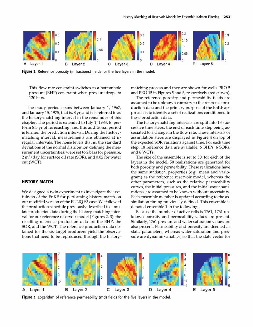
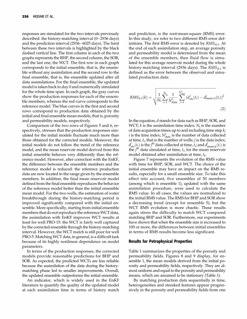
1. Layers 1, 3, and 5 correspond to fluvial channelsencased in flood-plain mudstone. They consist ofa low-porosity shale matrix (porosity <5%) withlinear streaks of high-porosity sand (porosity>20%). These two sandy and shaly facies are rep-resented by an ‘‘effective’’ facies with good reser-voir properties.

2. Layer 2 consists of marine or lagoonal shales withdistal mouth bars. This results in a low-porosityshaly matrix (porosity <5%) with a few higher po-rosity patches. Again, an effective facies with poorreservoir properties is used to represent this layer.

3. Layer 4 is a lagoonal delta, encased in lagoonal clay.It results in a low-porosity matrix (porosity <5%)with a more intermediate porosity region (porosity�15%). This layer is then populated by an effectivefacies with intermediate reservoir properties.

Reservoir Model

The numerical model is built over a 19 � 28 � 5 grid.The dimensions of each grid block in the X and Y di-rections are 180 � 180 m2 (1938 � 1938 ft2), and thethickness is defined according to the database data set.A total of 1761 active cells are present and the reser-voir is produced from six wells named PRO-1, PRO-4,PRO-5, PRO-11, PRO-12, and PRO-15. Figure 1 displaysthe top structure (layer 5) and the six well locations.

History Matching of Reservoir Models by Ensemble Kalman Filtering 251

The field is bounded by a fault to the east and southand by a strong aquifer to the west and north. Becauseof the strength of the aquifer, injection wells were notneeded for pressure maintenance.

Petrophysical Properties

Porosity and horizontal permeability realizations arestochastically drawn to populate the five layers of thereservoir, and their statistical properties are reportedin Table 1. Vertical permeability is assumed to be thesame as the horizontal one. The data used to generatethe realizations differed slightly from those providedby the PUNQ-S3 Web page (PUNQ-S3 test case, 2010)to enlarge the possible variations when performing sen-sitivity tests with the EnKF. In addition, the spatial var-iations in porosity and permeability are characterized

by a spherical variogram, whose main axes and anisot-ropy ratios are given in Table 1. All realizations (in-cluding the reference reservoir model) were generatedon the basis of the fast Fourier transformmoving averagealgorithm (Le Ravalec et al., 2000) without any condi-tioning to data at well locations. One of the resultingporosity and permeability models, which are used asthe reference models in this study, is displayed inFigures 2 and 3.

Production Schedule

The original PUNQ-S3 case involves three-phase flowsin the reservoir. In this chapter, we consider a simplertwo-phase (oil and water) black-oil case, which has theadvantage of providing more readable results. Theoriginal pressure-volume-temperature (PVT) dataweremodified to account for this change, whereas aquiferdata remained unchanged. Relative permeability wasgenerated according to the charts available in ourdatabase, and capillary pressure was assumed to be neg-ligible. We kept a production schedule similar to theone developed for the original model, which is thesame regardless of the production well. It consists ofthe following phases (Figure 4):

1. 1 yr of extended well testing with four 3-monthlyproduction periods with production rates of 100,200, 100, 50 m3/day, respectively;

2. 3 yr of well shut-in;3. 4 yr of production; a well shut-in test is performed

during the last 2 weeks of every year to collectshut-in pressure data. During the rest of the year, aconstant production rate of 100 m3/day is set up.

Figure 1. Top structure and well locations: PUNQ-S3 modelfrom the PUNQ-S3 Web page (PUNQ-S3 test case, 2010).GOC = gas-oil contact; OWC = for oil-water contact.

Table 1. Facies properties.*

Layer 1 2 3 4 5

Facies A B C D E

Porosity mean 0.1722 0.0802 0.1677 0.1615 0.1892Porosity variance 0.0078 0.0004 0.0050 0.0006 0.0049ln(kh) mean 2.18 1.41 2.24 2.47 2.49ln(kh) variance 3.14 0.74 3.26 5.64 3.72Correlationlength (m)

3500 750 6000 1500 3750

First anisotropyratio

0.286 1.0 0.25 0.50 0.333

Azimuth(degrees)

30 0 45 �30 60

*Porosity; logarithm of horizontal permeability, ln(kh); and vario-gram data.

252 HEIDARI ET AL.

This flow rate constraint switches to a bottomholepressure (BHP) constraint when pressure drops to120 bars.

The study period spans between January 1, 1967,and January 15, 1975, that is, 8 yr, and it is referred to asthe history-matching interval in the remainder of thischapter. The period is extended to July 1, 1983, to per-form 8.5 yr of forecasting, and this additional periodis termed the prediction interval. During the history-matching interval, measurements are obtained at ir-regular intervals. The noise levels that is, the standarddeviations of the normal distribution defining the mea-surement uncertainties, were set to 2 bars for pressure,2 m3/day for surface oil rate (SOR), and 0.02 for watercut (WCT).

HISTORY MATCH

We designed a twin experiment to investigate the use-fulness of the EnKF for performing history match onour modified version of the PUNQ-S3 case. We followedthe production schedule previously described to simu-late production data during the history-matching inter-val for our reference reservoir model (Figures 2, 3): theresulting reference production data are the BHP, theSOR, and the WCT. The reference production data ob-tained for the six target producers yield the observa-tions that need to be reproduced through the history-

matching process and they are shown for wells PRO-5and PRO-15 in Figures 5 and 6, respectively (red curves).

The reference porosity and permeability fields areassumed to be unknown contrary to the reference pro-duction data and the primary purpose of the EnKF ap-proach is to identify a set of realizations conditioned tothese production data.

The history-matching intervals are split into 13 suc-cessive time steps, the end of each time step being as-sociated to a change in the flow rate. These intervals orassimilation steps are displayed in Figure 4 on top ofthe expected SOR variations against time. For each timestep, 18 reference data are available: 6 BHPs, 6 SORs,and 6 WCTs.

The size of the ensemble is set to 50: for each of thelayers in the model, 50 realizations are generated forboth porosity and permeability. These realizations havethe same statistical properties (e.g., mean and vario-gram) as the reference reservoir model, whereas theother parameters, such as the relative permeabilitycurves, the initial pressures, and the initial water satu-rations, are assumed to be known without uncertainty.Each ensemble member is updated according to the as-similation timing previously defined. This ensemble isdenoted ensemble 1 in the following.

Because the number of active cells is 1761, 1761 un-known porosity and permeability values are present.Similarly, 1761 pressure and water saturation values arealso present. Permeability and porosity are deemed asstatic parameters, whereas water saturation and pres-sure are dynamic variables, so that the state vector for

Figure 2. Reference porosity (in fractions) fields for the five layers in the model.

Figure 3. Logarithm of reference permeability (md) fields for the five layers in the model.

History Matching of Reservoir Models by Ensemble Kalman Filtering 253

Figure 5. Production data simulated for well PRO-5 with an ensemble of size 50 during the history-matching and predictionperiods. First row: Initial ensemble. Second row: Final ensemble updated with the ensemble Kalman filter. The black dashedvertical line at 2936 days indicates the time limit between the history-matching interval (0–2936 days) and the predictioninterval (2936–6025 days). The gray curves correspond to the ensemble members, the red curves to the reference model, andthe blue curves to the results obtained with the reservoir model computed as the mean of the ensemble.

Figure 4. Evolution of the surfaceoil rate scheduled at the productionwells during the history-matchinginterval. The vertical red lines indi-cate the assimilation times.

254 HEIDARI ET AL.

the jth ensemble member at the kth time step is definedby

k;j ¼ ½transð�k;j;1Þ; . . . ;transð�k;j;NaÞ;transðkhk;j;1Þ; . . . ;

transðkhk;j;NaÞ;Pk;j;1; . . . ;Pk;j;Na

; Swk;j;1; . . . ;

Swk;j;Na;dk;j;1; . . . ;dk;j;Nd

�

Na is the total number of active grid blocks in the res-ervoir model and Nd is the total number of data. Thevariables �k;j;i, khk,j,i, Pk,j,i, and Swk,j,i are the porosity,horizontal permeability, pressure, andwater saturationin grid block i, respectively; dk,j,i stands for the i-threference production data, that is, BHP, SOR, or WCTfor the six production wells. Function trans defines a

transformation applied to state parameters, which en-sures that these parameters still have physical values atthe end of the updating step. These transformations are

1: Porosity transð�Þ ¼ log�

1� �

� �

2: Permeability transðkhÞ ¼ logðkhÞ

Results for Production Data

We now compare the performance of the initial withthe corrected models in terms of production data, thatis, BHP, SOR, and WCT, and focus on two wells: wellPRO-5 and well PRO-15 (Figures 5, 6). The production

Figure 6. Production data simulated for well PRO-15 with an ensemble of size 50 during the history-matching and predictionperiods. First row: Initial ensemble. Second row: Final ensemble updated with the ensemble Kalman filter. The black dashedvertical line at 2936 days indicates the time limit between the history-matching interval (0–2936 days) and the predictioninterval (2936–6025 days). The gray curves correspond to the ensemble members, the red curves to the reference model, andthe blue curves to the results obtained with the reservoir model computed as the mean of the ensemble.

ð1Þ

History Matching of Reservoir Models by Ensemble Kalman Filtering 255

responses are simulated for the two intervals previouslydescribed: the history-matching interval (0–2936 days)and the prediction interval (2936–6025 days). The limitbetween these two intervals is highlighted by the blackdashed vertical line. The first column in each of the twographs represents the BHP, the second column, the SOR,and the last one, the WCT. The first row in each graphcorresponds to the initial ensemble, that is, the ensem-ble without any assimilation and the second row to thefinal ensemble, that is, the ensemble updated after alldata assimilations. For the final ensemble, the updatedmodel is taken back to day 0 and numerically simulatedfor the whole time span. In each graph, the gray curvesshow the production responses for each of the ensem-ble members, whereas the red curve corresponds to thereference model. The blue curves in the first and secondrows correspond to production data obtained by theinitial and final ensemblemeanmodels, that is, porosityand permeability models, respectively.

Comparison of the two rows of Figures 5 and 6, re-spectively, stresses that the production responses sim-ulated for the initial models fluctuate much more thanthose obtained for the corrected models. Moreover, theinitial models do not follow the trend of the referencemodel, and the mean reservoir model derived from thisinitial ensemble behaves very differently than the ref-erence model. However, after correction with the EnKF,the difference between the ensemble members and thereference model is reduced: the reference productiondata are now located in the range given by the ensemblemembers. In addition, the final mean reservoir modeldefined from the final ensemble reproduces the behaviorof the reference model better than the initial ensemblemeanmodel. For the two wells, the estimation of waterbreakthrough during the history-matching period isimproved significantly compared with the initial en-semble.More specifically, starting from initial ensemblemembers that donot reproduce the referenceWCTdata,the assimilation with EnKF improves WCT results atleast for well PRO-15: the WCT is fairly well capturedby the corrected ensemble through the history-matchinginterval. However, theWCTmatch is still poor for wellPRO-5.MatchingWCTdata, in general, is a difficult taskbecause of its highly nonlinear dependence on modelparameters.

In terms of the production responses, the correctedmodels provide reasonable predictions for BHP andSOR. As expected, the predicted WCTs are less reliablebecause the assimilation of the data during the history-matching phase led to smaller improvements. Overall,the updated ensemble outperforms the initial ensemble.

An indicator, which is widely used in the EnKFliterature to quantify the quality of the updated modelat each assimilation time in terms of history match

and prediction, is the root-mean-square (RMS) error.In this study, we refer to two different RMS error def-initions. The first RMS error is denoted by RMSd,1. Atthe end of each assimilation step, an average porosityand permeability model is determined from the meanof the ensemble members, then fluid flow is simu-lated for this average reservoir model during the wholehistory-matching interval (2936 days). The RMSd,1 isdefined as the error between the observed and simu-lated production data:

RMSd;1ðkÞ ¼

ffiffiffiffiffiffiffiffiffiffiffiffiffiffiffiffiffiffiffiffiffiffiffiffiffiffiffiffiffiffiffiffiffiffiffiffiffiffiffiffiffiffiffiffiffiffiffiffiffiffiffiffiffiffiffiffiffiffiffiffiffiffiffiffiffiffiffiffiffiffi1

Nt

XNt

i¼1

1

Ntidata

XNtidata

j¼1

ðdjobsðtiÞ � d

jmean;k

vuuut ðtiÞÞ2

ð2Þ

In the equation, d stands for data such as BHP, SOR, andWCT; k is the assimilation time index; Nt is the numberof data acquisition times up to and including time step k;i is the time index; Nt

data is the number of data collectedat time, ti, that is the number of wells; j is the data index;djobsðtiÞ is the j

th data collected at time, ti; and djmean;kðtiÞ is

the jth data simulated at time, ti, for the mean reservoirmodel obtained after assimilation at time, tk.

Figure 7 represents the evolution of the RMS valuewith time for BHP, SOR, and WCT. The choice of theinitial ensemble may have an impact on the RMS re-sults, especially for a small ensemble size. To take thiseffect into account, five ensembles of 50 members(among which is ensemble 1), updated with the sameassimilation procedure, were used to calculate theRMS value. In all cases, the values are normalized tothe initial RMS value. The RMS for BHP and SOR showa decreasing trend (except for ensemble 5), but theWCT RMS evolution is more chaotic. These resultsagain stress the difficulty to match WCT comparedmatching BHP and SOR. Furthermore, our experimentshave shown that when the ensemble size is increased to100 or more, the differences between initial ensemblesin terms of RMS results become less significant.

Results for Petrophysical Properties

Table 1 summarizes the properties of the porosity andpermeability fields. Figures 8 and 9 display, for en-semble 1, the mean models derived from the initial po-rosity and permeability fields, respectively. They are al-most uniform and equal to the porosity andpermeabilitymeans, which are assumed to be stationary (Table 1).

By matching production data sequentially in time,heterogeneities and streaked features appear progres-sively in the porosity and permeability fields from one

256 HEIDARI ET AL.

assimilation time to the next. Figures 10 and 11 showthe mean corrected porosity and permeability modelsafter performing 13 assimilations, that is, 13 successivehistory matches of production data. The main featuresof the reference model (low- and high-porosity andpermeability streaks in layers 1, 3, and 5, togetherwith low- and high-porosity and permeability patchesin layers 2 and 4) are retrieved in the corrected models.The porosity fields for layers 1, 3, and 5 were over-estimated (the porosity values were expected to belower than 0.35; they were trimmed when higher).

The overestimation is less significant for permeabilityfields; the updated fields are on the same order of mag-nitude as the reference model. Gao et al. (2006) relatedthe overestimation problem to the constraints on wellpressures and SORs in the fluid-flow simulation andreduced it by removing the bounds on the well BHP.This problem is mentioned in other applications of theEnKF (Gu and Oliver, 2005). According to Devegowdaet al. (2007), the overestimation is a result of the spu-rious correlations in the covariance matrix because ofthe finite ensemble size. They proposed a mitigation

Figure 7. The first root-mean-square error (RMSd,1) of production data. (A) Bottomhole pressure, (B) surface oil rate, and(C) water cut for five ensembles of size 50. The values are normalized on the initial value (t = 0).

Figure 8. Mean of initial ensemble for porosity distribution in the five layers.

History Matching of Reservoir Models by Ensemble Kalman Filtering 257

strategy by covariance localization. This is beyond thescope of this chapter.

It can also be shown that the assimilation processinduces a decrease in the variance of the porosity andpermeability ensemble members, especially aroundwell locations. As wells are perforated in layers 3, 4,and 5, variance reduction is more significant in theselayers than in layers 1 and 2. Figures 12 and 13 display,for ensemble 1, the variance computed for the porosityand permeability models in layer 4. The first graphgives the variance for the initial ensemble, the middleone for the ensemble obtained after seven assimila-tions and the last one for the final ensemble (13 assim-ilations). Although variability reduction is a naturalconsequence of data assimilation, the updated ensem-ble should be representative of the variability of modelparameters. Hence, excessive variance reduction shouldbe avoided. This can be ensured using a larger ensem-ble. Moreover, the model noise is neglected in petro-leum applications of the EnKF, and its inclusion mayhelp mitigate this problem.

The distance between the assimilated porosity andpermeability models for each ensemble member andthe corresponding reference models is quantified bythe following static RMS error:

RMSsðkÞ ¼

ffiffiffiffiffiffiffiffiffiffiffiffiffiffiffiffiffiffiffiffiffiffiffiffiffiffiffiffiffiffiffiffiffiffiffiffiffiffiffiffiffiffiffiffiffiffiffiffiffiffiffiffiffiffiffi1

Ne

XNe

j¼1

1

Na

XNa

i¼1

ðyj;i � yref ;iÞ2vuut ð3Þ

Subscript s stands for static (reservoir parameters areregarded as static data), Na is the number of active

grid blocks, i the grid block index, and j the ensemblemember number. In addition, yj,i is the value of eitherthe porosity or permeability logarithm attributed to thegrid block i for the ensemble member j, and yref,i is thereference value of this property. This RMS value quan-tifies the convergence toward the reference reservoirparameters or static data. Figure 14 shows, for ensem-ble 1, the static RMS values computed after each assi-milation for porosity and horizontal permeability loga-rithm in the five layers (all values are normalized tothe static RMS values computed at time 0). A decreas-ing trend is evident for most of the parameters, exceptfor porosity in layers 1, 3, and 5. As previously ex-plained, these layers control most of the flow, and theirupdated porosities were overestimated. The effect ofthe initial ensemble was also studied on the RMS value:although the RMS values are not the same for all en-sembles, the same trend was observed for differentensembles of size 50.

SENSITIVITY ANALYSIS

The performance of EnKF for history match and pre-diction depends on several parameters, among whichensemble size, measurement data uncertainty, assim-ilation time step, and choice of the initial ensemble areimportant. A set of experiments illustrates the influ-ence of these parameters on the results. To reducethe effect of the initial ensembles on the experimentsdedicated to the influence of ensemble size, data un-certainty, and assimilation time step, five different

Figure 9. Mean of initial ensemble for permeability (ln[kh]) distribution in the five layers.

Figure 10. Mean of final ensemble for porosity distribution in the five layers.

258 HEIDARI ET AL.

ensembles are generated for the target parameter, andthe same assimilation process is performed for each ofthem. The RMS values presented hereafter are the av-erage values of the RMS results obtained for the fiveensembles.

Ensemble Size

The EnKF provides an approximation of the error co-variance matrix from an ensemble of finite size. As thesize of the ensemble, Ne, increases, the approximationof the error covariancematrix improves proportionallyto 1=

ffiffiffiffiN

p. Therefore, spurious correlations in the co-

variance matrix are reduced. However, increasing theensemble size induces a larger fluid-flow simulationand computational overburden. Thus, a trade-off existsbetween the accuracy of the covariance matrix approx-imation and the computational cost, and the choice ofthe ensemble size is case dependent.Weapply the EnKFto the same case study as in the previous section butusing ensembles of size 50, 100, 200, and 500. We con-sider the same data uncertainties as previously dis-cussed. The assimilation intervals are reported by thered dashed vertical lines in Figure 4.

Two metrics quantify the performance of the differ-ent ensembles: the static RMS (RMSs) previously in-troduced and the dynamic RMS, denoted by RMSd,2.This quantity assesses the performance of EnKF atthe end of each time step by calculating, for each of theensemble members, the difference between the updatedproduction responses (BHP, SOR, and WCT) and the

reference production data for the same time step. ThisRMS is written as

RMSd;2 ¼

ffiffiffiffiffiffiffiffiffiffiffiffiffiffiffiffiffiffiffiffiffiffiffiffiffiffiffiffiffiffiffiffiffiffiffiffiffiffiffiffiffiffiffiffiffiffiffiffiffiffiffiffiffiffiffiffiffiffiffiffiffiffiffiffiffiffiffiffiffiffiffiffiffiffiffiffiffiffiffiffiffiffiffiffi1

Ne

XNe

i¼1

1

Nt

XNt

j¼1

1

Ntjdata

XNtj

data

k¼1

ðdkobsðtjÞ � dki ðtjÞÞ2

vuuut

ð4Þ

Ne is the ensemble size. All other variables were pre-viously defined. The RMSd,2 value can be calculated foreach of the target production responses BHP, SOR, orWCT separately, or for all of them together with respectto their uncertainties.

Table 2 provides the RMSd,2 values determined fordifferent ensemble sizes. The values are normalized tothe average RMS obtained for the ensembles of size 50.At first glance, it seems that increasing the ensemblesize from 50 to 100 decreases the RMS value. A largerincrease in the ensemble size has a less significant ef-fect. Therefore, an ensemble of size 100 is more appro-priate considering central processing unit (CPU) costs.

Table 3 provides the RMSs values for ensembles ofincreasing size. These values are normalized by the av-erage RMS error determined for the ensembles of size50. The larger the ensemble size, the lower the RMSerror for most of the static properties. Furthermore, in-creasing the ensemble size from 200 to 500 reduces thestatic RMS error, but less so than when passing from 50to 100 or 200. Thus, an ensemble of size 100 to 200 iswellsuited for the considered problem.

Figure 11. Mean of final ensemble for permeability (ln[kh]) distribution in the five layers.

Figure 12. Variance of the en-semble for the porosity field inlayer 4: (A) Initial ensemble,(B) intermediate ensemble, and(C) final ensemble.

History Matching of Reservoir Models by Ensemble Kalman Filtering 259

Data Uncertainty

We now assess the effect of measurement uncertaintyon the performance of the EnKF. Under the uncer-tainty 1 case, data uncertainties were set to 2 bars forBHP, 2 m3/day for SOR, and 0.02 for WCT. Theuncertainty 2 case assumes an error of 3 bars for BHP,3 m3/day for SOR, and 0.03 for WCT. The quality of the

results is again measured by the RMSd,2 error (equa-tion 4). The results presented in Table 4 are normal-ized to the average RMS value obtained for the ensem-bles of size 50 and the uncertainty 1 setting to make thecomparison of results easier. In the uncertainty 2 con-figuration, the RMS errors computed for the productiondata are increased in comparison with uncertainty 1 fora given ensemble size. Apart from the ensembles of

Figure 14. Static root-mean-square (RMS) values for the porosity and horizontal permeability log (ln[kh]) in layers 1 to 5. Thevalues are normalized on the initial time (t = 0).

Figure 13. Variance of the en-semble for permeability fieldin layer 4: (A) Initial ensemble,(B) intermediate ensemble, and(C) final ensemble.

260 HEIDARI ET AL.

size 50, our experiment demonstrates that even with ahigher measurement of uncertainty, the final ensem-bles outperform the initial ensembles.

Haugen et al. (2008) have also performed a sensi-tivity test on measurement uncertainties for an ap-plication of the EnKF on a North Sea field case. Theyclaimed that the choice of the measurement uncertain-ty is less important; assimilations with increased anddecreased levels of uncertainty provided improved es-timates compared with the initial reservoir models.They did not quantitatively compare the results.

Assimilation Step

The time interval between two consecutive assimila-tions is also an important issue for practical EnKF ap-plications. Smaller assimilation steps may be requiredto capture significant perturbations or nonlinearitiesin fluid flow. These perturbations are induced by addi-tion of a well or variations in flow rates.

The production scheme followed for this case studyinvolves several changes in the flow rate. Therefore,we compare the performance of the EnKF for twodistinct time step settings. The first assimilation timepartitioning, time step 1, is reported in Figure 4. Inthe second partitioning, time step 2, each of the pre-vious time steps is divided in two smaller steps. Weconsidered ensembles of size 50, 100, and 200 for theuncertainty 1 metric.

Results are compared using the RMSd,2 error metric(equation 4). The RMS errors reported in Table 5 arenormalized to the average RMS values determined forthe ensembles of size 50 with the time step 1 setting.Keeping the ensemble size constant while decreasingthe time step size makes the RMS smaller for the tar-get production responses. Also, decreasing the timestep size while increasing the ensemble size contrib-utes even more to improve the match.

Choice of the Initial Ensemble

One of the main issues with EnKF is the choice of theinitial ensemble because different initial ensemblesresult in different RMS values for production data,

Table 2. Effect of ensemble size.*

Ensemble Size

Property 50 100 200 500

BHP** 1 0.33 0.27 0.25SOR** 1 0.29 0.19 0.17WCT** 1 0.44 0.44 0.41All 1 0.34 0.30 0.26

*Average value of the dynamic RMSd,2 obtained with several en-sembles of increasing size, normalized on the value obtained withan ensemble size of 50.**BHP = bottomhole pressure; SOR = surface oil rate; WCT = watercut.

Table 3. Effect of ensemble size.*

Ensemble Size

Property 50 100 200 500

Phi-L1 1 0.62 0.55 0.54Phi-L2 1 0.74 0.68 0.66Phi-L3 1 0.72 0.64 0.64Phi-L4 1 0.67 0.64 0.65Phi-L5 1 0.62 0.67 0.65Ln(kh)-L1 1 0.67 0.66 0.61Ln(kh)-L2 1 0.77 0.69 0.68Ln(kh)-L3 1 0.83 0.69 0.72Ln(kh)-L4 1 0.81 0.77 0.74Ln(kh)-L5 1 0.71 0.71 0.65

*Average value of the static root-mean-square obtained with severalensembles of increasing size, normalized on the value obtained withan ensemble size of 50.

Table 4. Effect of measurement uncertainty.*

Uncertainty 1 Uncertainty 2

Ensemble size 50 100 200 50 100 200BHP** 1 0.33 0.27 1.26 0.70 0.61SOR** 1 0.29 0.19 1.11 0.49 0.37WCT** 1 0.44 0.44 1.02 0.98 0.96All 1 0.34 0.30 1.11 0.62 0.54

*Average value of the dynamic RMSd,2 obtained with two increasinglevels of uncertainty and several ensembles of increasing size, nor-malized on the value obtained with an ensemble size of 50.**BHP = bottomhole pressure; SOR = surface oil rate; WCT = watercut.

Table 5. Effect of assimilation interval.*

Time Step 1 Time Step 2

Ensemble size 50 100 200 50 100 200BHP** 1 0.33 0.27 0.60 0.28 0.24SOR** 1 0.29 0.19 0.56 0.21 0.15WCT** 1 0.44 0.44 0.50 0.35 0.29All 1 0.34 0.30 0.54 0.27 0.22

*Average value of the dynamic RMSd,2 obtained with two decreasingsets of assimilation time intervals and several ensembles of increasingsize, normalized on the value obtained with an ensemble size of 50.**BHP = bottomhole pressure; SOR = surface oil rate; WCT = watercut.

History Matching of Reservoir Models by Ensemble Kalman Filtering 261

indicating the importance of the initial ensemble in thequality of history match and predictions. Initial ensem-bles are generated stochastically and filter performancemay change from one ensemble to another (Lorentzenet al., 2005). Moreover, ensemble members becomehighly correlated after assimilation. This phenomenonis a well-known problem of Markov Chain–MonteCarlo methods. To mitigate these limitations, Thulinet al. (2008) recommended performing several EnKFruns with an appropriate small ensemble size andclaimed that the results would be superior to thoseobtained by only one large ensemble.

How does the EnKF perform in terms of predictioncapability with different ensembles of identical size?

Focusing on cumulative oil production, ten differentensembles of size 100 were generated using the uncer-tainty 1 and time step 1 framework. The forecast ca-pability of each of the ensembles is assessed by com-paring the total cumulative oil production from theinitial value with that of the final updated ensemblesfor the whole history-matching and prediction inter-vals. To make the comparison meaningful, the updatedmodels obtained at the end of the history-matching in-terval (0–2936 days) were simulated from day 0 to theend of the prediction interval. The results are plotted inFigure 15.

The reference oil data are in the range provided bythe initial ensembles, more specifically between the

Figure 15. Box plot of cumulative oil production for 10 ensembles of size 100: (A) initial ensemble, (B) final ensemble. Theblack horizontal line corresponds to the cumulative oil production for the reference reservoir model at the end of 6025 days ofproduction. Each box is limited by the lower and upper quartiles, and the red line within each box shows the median value.The small black lines (whiskers) show the extent of the data for each box plot. Red plus signs are outliers of each data set.

262 HEIDARI ET AL.

upper quartile and the upper extent for the data. Themedian predicted oil cumulative production is far fromthe true one and the spread, that is, P(75) to P(25), foreach ensemble is fairly high. After assimilating the datain the history-matching interval, the spread is reducedand the true cumulative oil production value is betterpositioned within the forecasted ranges. Moreover, thedifference between the median and true cumulativeoil production is significantly smaller, and one-half ofthe ensembles include the true value between the lowerandupperquartiles, that is, P(75) toP(25).Considering therange of predictions by the 10 ensembles, we suggestthat soundpredictions should be based on several ensem-bles of appropriate size, similar to what was suggestedby Lorentzen et al. (2005) and Thulin et al. (2008).

CONCLUSIONS

The ease of implementation and low computationalcost make the EnKF method appealing for most history-matching studies. Although the applications are gener-ally successful, the fundamental assumptions intrinsicto EnKF theorymaybe problematic, althoughmitigationstrategies were suggested in the literature to improvethe performance. In this chapter, we focus on the useof the EnKFmethod for performing historymatch anduncertainty quantification. A fairly small ensemble ofsize 50 is used to provide the initial uncertainty in po-rosity and permeability. By sequentially matching theproduction data (BHP, SOR, and WCT), porosity andpermeability fields were gradually adjusted so as to re-produce the reference production data. The WCT wasshown to be quite difficult tomatch possibly because ofthe highly nonlinear dependence of these data to res-ervoir parameters.

We also performed a set of sensitivity tests to as-sess the function of some EnKF parameters in history-matching results: the ensemble size, the data uncer-tainty, the assimilation time step, and the choice ofthe initial ensemble. The following conclusions can bedrawn:

1. Increasing the ensemble size results in a bettermatch for the production data (BHP, SOR, andWCT), but there exists a trade-off between the in-crease in computation time and the improvementsin the results. Our experiments suggest that anensemble size of 100 to 200 is appropriate to ob-tain acceptable results with EnKF. However, thisnumber is case dependent.

2. The level of uncertainty in measured data is of lesssignificance; data assimilationwith EnKF improves

model estimates whenever the size of the ensembleis large enough.

3. Decreasing the assimilation time step is requiredto better capture the abrupt changes in dynamicsof the model.

4. The match of cumulative oil production is betterassessed when estimated from several ensemblesof identical size, although this makes the processmore CPU time consuming.

REFERENCES CITED

Anderson, J. L., 2001, An ensemble adjustment filter for dataassimilation: Monthly Weather Review, v. 129, p. 2884–2903, doi:10.1175/1520-0493(2001)129<2884:AEAKFF>2.0.CO;2.

Anderson, J. L., 2007, Exploring the need for localization inensemble data assimilation using a hierarchical ensemblefilter: Physica D, v. 230, p. 99–111, doi:10.1016/j.physd.2006.02.011.

Aziz, K., and A. Settari, 1979, Petroleum reservoir simula-tion: London, U.K., Applied Science, 497 p.

Bertino, L., G. Evensen, and H. Wackernagel, 2003, Sequentialdata assimilation techniques in oceanography: Interna-tional Statistical Review, v. 71, no. 2, p. 223–241, doi:10.1111/j.1751-5823.2003.tb00194.x.

Burgers, G., P. J. van Leeuwen, and G. Evensen, 1998, Anal-ysis scheme in the ensemble Kalman filter: MonthlyWeather Review, v. 126, p. 1719–1724, doi:10.1175/1520-0493(1998)126<1719:ASITEK>2.0.CO;2.

Chen, Y., D. S. Oliver, and D. Zhang, 2009, Data assimilationfor nonlinear problems by ensemble Kalman filter withreparameterization: Journal of Petroleum Science and En-gineering, v. 66, p. 1–14, doi:10.1016/j.petrol.2008.12.002.

Cohn, S. E., 1997, An introduction to estimation theory:Journal of the Meteorological Society of Japan, v. 75,p. 257–288.

Devegowda, D., E. Arroyo-Negrete, A. Datta-Gupta, andS. G. Douma, 2007, Efficient and robust reservoir modelupdating using ensemble Kalman filter with sensitivity-based covariance localization: SPE Reservoir SimulationSymposium, February 26–28, 2007, Houston, Texas, SPEpaper 106144, 14 p.

Evensen, G., 1994, Sequential data assimilation with a non-linear quasi-geotrophic model using Monte Carlo meth-ods to forecast error statistics: Journal of GeophysicalResearch Ocean, v. 99, no. C5, p. 10,143–10,162, doi:10.1029/94JC00572.

Evensen, G., 2007, Data assimilation: The ensemble Kalmanfilter: Berlin, Germany, Springer, 307 p.

Evensen, G., and P. J. van Leeuwen, 1996, Assimilation ofgeosat altimeter data for the Agulhas current using theensemble Kalman filter with a quasigeostraphic model:Monthly Weather Review, v. 124, p. 85–96, doi:10.1175/1520-0493(1996)124<0085:AOGADF>2.0.CO;2.

Evensen, G., H. Hove, H. C. Meisingset, E. Reiso, and Ø.

History Matching of Reservoir Models by Ensemble Kalman Filtering 263

Espelid, 2007, Using the EnKF for assisted history matchingof a North Sea reservoir model: SPE Reservoir SimulationSymposium, February 26–28, 2007, Houston, Texas, SPEpaper 106184, 13 p.

Fertig, E., B. R. Hunt, E. Ott, and I. Szunyogh, 2007, As-similating nonlocal observations with a local ensembleKalman filter: Tellus, v. 59A, p. 719–730.

Floris, F. J. T., M. D. Bush, M. Cuypers, F. Roggero, and A. R.Syversveen, 2001, Methods for quantifying the uncer-tainty of production forecasts: A comparative study: Pe-troleum Geoscience, v. 7, p. 87–96.

Gao, G., M. Zafari, and A. C. Reynolds, 2006, Quantifyinguncertainty for the PUNQ-S3 problem in a Bayesian set-tingwith RML and EnKF: SPE Journal, v. 11, no. 4, p. 506–515.

Gu, Y., and D. S. Oliver, 2005, History Matching of the PUNQ-S3 reservoir model using the ensemble Kalman filter: SPEJournal, v. 10, p. 217–224.

Gu, Y., and D. S. Oliver, 2007, An iterative ensemble Kalmanfilter for multiphase fluid flow data assimilation: SPEJournal, v. 12, no. 4, p. 438–446.

Hamill, T. M., and J. S. Whitaker, 2001, Distance-dependentfiltering of background error covariance estimate in anensemble Kalman filter: Monthly Weather Review, v. 129,p. 2776–2790, doi:10.1175/1520-0493(2001)129<2776:DDFOBE>2.0.CO;2.

Haugen, V., and G. Evensen, 2002, Assimilation of SLAand SST data into OGCM for the Indian Ocean: Ocean Dy-namics, v. 52, p. 133–151, doi:10.1007/s10236-002-0014-7.

Haugen, V., L. Natvik, G. Evensen, A. Berg, K. Flornes, andG. Naevdal, 2008, History matching using the ensembleKalman filter on a North Sea field case: SPE Journal, v. 13,no. 4, p. 382–391.

Houtekamer, P., and H. L. Mitchell, 1998, Data assimila-tion using an ensemble Kalman filter technique: MonthlyWeather Review, v. 126, no. 3, p. 796–811, doi:10.1175/1520-0493(1998)126<0796:DAUAEK>2.0.CO;2.

Houtekamer, P., and H. L. Mitchell, 2001, A sequential en-semble Kalman filter for atmospheric data assimilation:Monthly Weather Review, v. 129, p. 123–137, doi:10.1175/1520-0493(2001)129<0123:ASEKFF>2.0.CO;2.

Kalman, R. E., 1960, A new approach to linear filtering andprediction problems: Transactions of the American So-ciety of Mechanical Engineers–Journal of Basic Engineer-ing, v. 82, p. 35–45.

Le Ravalec, M., B. Noetinger, and L. Y. Hu, 2000, The FFTmoving average (FFT-MA) generator: An efficient numer-ical method for generating and conditioning Gaussian sim-ulations: Mathematical Geology, v. 32, no. 6, p. 701–723,doi:10.1023/A:1007542406333.

Li, G., and A. C. Reynolds, 2007, An iterative ensemble Kalmanfilter for data assimilation: SPE Annual Technical Confer-ence and Exhibition, November 11–14, 2007, Anaheim,California, SPE paper 109808, 18 p.

Liu, N., and D. S. Oliver, 2005, Critical evaluation of the en-semble Kalman filter on history matching of geologic fa-

cies: SPE Reservoir Evaluation and Engineering, v. 8, no. 6,p. 470–477.

Lorenc, A. C., 1986, Analysis methods for numerical weath-er prediction: Quarterly Journal of the Royal Meteorolog-ical Society, v. 112, no. 474, p. 1177–1194, doi:10.1002/qj.49711247414.

Lorentzen, R. J., G. Naevdal, B. Valles, A. N. Berg, and A. A.Grimstad, 2005, Analysis of the ensemble Kalman filterfor estimation of permeability and porosity in reservoirmodels: SPE Annual Technical Conference and Exhibi-tion, October 9–12, 2005, Dallas, Texas, SPE paper 96375,10 p.

Margulis, S. A., D. McLaughlin, D. Entekhabi, and S. Dunne,2002, Land data assimilation and estimation of soil mois-ture using measurements from the Southern Great Plains1997 field experiment: Water Resources Research, v. 38,no. 12, p. 35.1–35.18.

Moreno,D., S. I. Aanonsen, G. Evensen, J. A. Skjervheim, 2008,Channel facies estimation based on Gaussian perturba-tions in the EnKF: European Association of Geoscientistsand Engineers 11th European Conference on the Math-ematics of Oil Recovery, September 8–11, 2008, Bergen,Norway.

Naevdal, G.,T. Mannseth, and E. H. Vefring, 2002, Near-wellreservoir monitoring through ensemble Kalman filter:SPE/DOE Improved Oil Recovery Symposium, April 13–17, 2002, Tulsa, Oklahoma, SPE paper 75235, 9 p.

PumaFlow, 2007, Reference Manual Release 2.0, September,BeicipFranlab–Institut Francais du Petrole.

PUNQ-S3 test case, 2010: http://www3.imperial.ac.uk/earthscienceandengineering/research/perm/punq-s3model/onlinedataset (accessed May 1, 2009).

Thulin, K., G. Naevdal, and S. I. Aanonsen, 2008, QuantifyingMonte Carlo uncertainty in the ensemble Kalman filter:11th European Conference on the Mathematics of Oil Re-covery, September 8–11, 2008, Bergen, Norway.

Vabø, J. G., G. Evensen, J. Hove, and J. A. Skjervheim, 2008,Using the EnKF with kernel methods for estimation ofnon-Gaussian variables: European Association of Geo-scientists and Engineers 11th European Conference on theMathematics of Oil Recovery, September 8–11, 2008,Bergen, Norway.

Wang, X., T. M. Hamill, J. S. Whitaker, and C. H. Bishop,2007, A comparison of hybrid ensemble transform Kalmanfilter: Optimum interpolation and ensemble square rootfilter analysis schemes: Monthly Weather Review, v. 135,no. 3, p. 1055–1076, doi:10.1175/MWR3307.1.

Wen, X.-H., and W. H. Chen, 2007, Some practical issueson real-time reservoir model updating using ensembleKalman filter: SPE Journal, v. 12, no. 2, p. 156–166.

Wunsch, C., 1996, The ocean circulation inverse problem:New York, Cambridge University Press, 437 p.

Zafari, M., and A. C. Reynolds, 2007, Assessing the uncer-tainty in reservoir description and performance predic-tions with the ensemble Kalman filter: Society of Petro-leum Engineering Journal, v. 12, no. 3, p. 382–391.

264 HEIDARI ET AL.