numerical modelling and automated history matching in … · predicting the reservoir performance...
TRANSCRIPT

Master Thesis
Numerical modelling and automated history matching in SCAL for improved data quality Written by: Advisor: Bettina Jenei, BSc Univ.-Prof. Dipl.-Phys. Dr.rer.nat. Holger OTT m1435380 Mat.Inz. Roman Manasipov
Leoben, 30.01.2017

i
EIDESSTATTLICHE ERKLÄRUNG
Ich erkläre an Eides statt, dass ich die vorliegende Diplomarbeit selbständig und ohne fremde Hilfe verfasst, andere als die angegebenen Quellen und Hilfsmittel nicht benutzt und die den benutzten Quellen wörtlich und inhaltlich entnommenen Stellen als solche erkenntlich gemacht habe.

ii
AFFIDAVIT
I hereby declare that the content of this work is my own composition and has not been submitted previously for any higher degree. All extracts have been distinguished using quoted references and all information sources have been acknowledged.

iii
Kurzfassung
Relative Permeabilitäts- und Kapillardrucksättigungsfunktionen sind für das Reservoir Engineering von wesentlicher Bedeutung, da sie die Verdrängungseffizienz einer zwei-Phasen Strömung – z.B. durch Wasserinjektion – auf der mikroskopischen und makroskopischen Skala bestimmt. Diese Funktionen sind zur Vorhersage der Produktion während der gesamte Lebensdauer eines Reservoirs von Bedeutung. Relative Permeabilität und Kapillardruck können im Labor durch Kernflutung bestimmt werden. Interpretiert werden die Daten in der Regel mittels analytischer Modelle, die jedoch nur unter bestimmten Voraussetzungen die Experimente genau beschreiben. In realen Experimenten sind diese Voraussetzungen jedoch oft noch hinreichend erfüllt, was systematische Fehler nach sich zieht. Es ist deshalb empfehlenswert (allerdings selten durchgeführt) SCAL (special core analysis) Experimente (speziell von Servicelaboratorien durchgeführte) mittels numerischer Modelle zu interpretieren.
Das Hauptproblem analytischer Ansätze sind die groben Annahmen hinter den Interpretationsmodellen, die nötig sind um die Gleichungen analytisch zu lösen. So wird zum Beispiel beim JBN-Ansatz [1] die die Wirkung von Kapillarkräften vernachlässigt, was vor allem ein Problem nahe der Restölsättigung ist. Trotz der Stärke analytischer Modelle, kann in numerischen Modellen die volle Physik berücksichtigt werden, was zu einer höheren Verlässlichkeit der Ergebnisse führt, was das Ziel der vorliegenden Arbeit ist. Dabei werden die Produktions-, Druck- und Sättigungsdaten von Steady-State, Unsteady State und Zentrifugen Experimenten gemeinsam interpretiert und somit genauere Ergebnisse erzielt. Schließlich wird das Verfahren durch Vergleich der in dieser Studie erhaltenen Ergebnisse mit Literaturdaten verglichen, die durch die Verwendung verschiedener Simulationswerkzeuge und -ansätze erhalten wurden.
Die Masterarbeit zielt auf die numerische Interpretation von SCAL Daten, um die Qualität der relativen Permeabilität und der Kapillardrucksättigungsfunktionen zu verbessern. Im Rahmen der Arbeit werden numerische Modelle für verschiedene SCAL Techniken erarbeitet und experimentelle Daten werden analysiert. Um eine bessere und objektive Interpretation zu gewährleisten und für eine bessere Handhabung der Daten, wird das Analyseverfahren automatisiert.

iv
Abstract
Relative permeability and capillary pressure saturation functions are essential to Reservoir Engineering because they determine the efficiency of water-flooding operations on the microscopic and macroscopic scale. These functions are required for predicting the reservoir performance through the whole reservoir life time. Generally, the relative fluid-phase permeability in the formation rock can be measured by performing displacement experiments in core sample by either steady state or unsteady state flooding experiments.
Conventional analytical interpretation of laboratory SCAL experiments as performed by many service laboratories may add uncertainty to relative permeability and capillary pressure data and consequently to reservoir simulation. Relative permeability and capillary pressure function can more reliably be obtained by numerical history matching of displacement experiments.
The main problems of the analytical approach are the crude approximations behind the interpretation models such as the JBN approach [1]. This is the restrictive assumption that neglects action of capillary forces, which is especially a problem close to residual oil saturation. Thus numerical modelling of SS (steady-state), USS (unsteady state) and C (centrifuge) experiments and more specifically history matching of related production, pressure and saturation data are the way to obtain more accurate results because full physics is taken into account. Finally, the procedure will be verified by comparing the results obtained in this study to literature data obtained by using different simulation tools and approaches.
The proposed master thesis aims on numerical interpretation of SCAL (Special Core Analysis) data in order to improve the quality of relative permeability and capillary pressure saturation functions.
By simulating and history matching SCAL experiments we will overcome typical experimental issues and the deficiencies of analytical interpretation methods. In the frame of the thesis, numerical models for different SCAL techniques will be setup and experimental data will be described. To achieve the best and a more objective interpretation and for better data handling, the history matching procedure will be automated.

v
List of Tables
Table 7.1: Fluid and rock properties of SS imbibition measurement; taken from [7]. ....63
Table 7.2: Injection schedule for Steady State measurement ......................................63
Table 7.3: SS Simulated Corey parameters of Relative Permeability ..........................69
Table 7.4: Fluid and rock properties of USS imbibition measurement ..........................70
Table 7.5: Injection schedule for Unsteady-State measurement ..................................70
Table 7.6: USS Simulated Corey parameters of Relative Permeability ........................73
Table 7.7: Fluid and rock properties of Centrifuge imbibition measurement .................75
Table 7.8: Rotation schedule for Centrifuge measurement ..........................................75
Table 7.9 : C Simulated Corey parameters of Relative Permeability ............................79
Table 7.10: C Simulated Extended Corey parameters of Capillary Pressure ...............80

vi
List of Figures
Figure 1.1: Overall workflow of the Reservoir Simulation [2] ......................................... 1
Figure 1.2: Workflow of the SCAL data [4] .................................................................... 2
Figure 2.1: REV (Representative Elementary Volume) in terms of porosity [6] ............. 5
Figure 2.2: Contact angle definition in water-mercury system on glass surface ............ 7
Figure 2.3: Schematic figure of wetting and non-wetting fluids ..................................... 8
Figure 2.4: Schematic figure of the Darcy´s law ........................................................... 8
Figure 2.5: Typical relative permeability curves of oil and water in water-wet system ..14
Figure 2.6: Typical relative permeability curves based on wettability [2] ......................16
Figure 2.7: Typical fractional flow curve [8] ..................................................................17
Figure 2.8: Capillary hysteresis [9] ..............................................................................21
Figure 2.9: Schematic figure of the capillary hysteresis in a water wet system, Curve: 1: drainage (water displaced by oil), Curve 2: imbibition (oil displaced by water) ......22
Figure 2.10: Equilibrium between gravity and capillary forces [2].................................22
Figure 3.1: Laboratory apparatus for SS relative permeability measurements [4] ........24
Figure 3.2: Automated centrifuge system at imbibition and drainage setup [4] ............28
Figure 5.1: Schematic figure of the SS core model in above view ...............................39
Figure 5.2: Schematic figure of the USS core model in above view .............................40
Figure 5.3: Schematic figure of the Centrifuge core model in front view with initial saturations ...........................................................................................................42
Figure 6.1: Case 1 – Calculated differential pressure in SS measurement with smooth Pc curve ...............................................................................................................45
Figure 6.2: Case 1 – Calculated cumulative oil production of SS measurement with smooth Pc curve ..................................................................................................46
Figure 6.3: Case 1 – Calculated average water saturation in SS measurement with smooth Pc curve ..................................................................................................46
Figure 6.4: Case 2 – Calculated differential pressure in SS measurement with smooth Pc curve ...............................................................................................................47
Figure 6.5: Case 2 – Calculated cumulative oil production of SS measurement with sharp Pc curve .....................................................................................................48
Figure 6.6: Case 2 – Calculated average water saturation in SS measurement with sharp Pc curve .....................................................................................................48

vii
Figure 6.7: Case 3 – Calculated differential pressure in USS measurement with smooth Pc curve ...............................................................................................................49
Figure 6.8: Case 3 –– Calculated cumulative oil production of USS measurement with smooth Pc curve ..................................................................................................50
Figure 6.9: Case 3 – Calculated average water saturation in USS measurement with smooth Pc curve ..................................................................................................50
Figure 6.10 Case 4 – Calculated differential pressure in USS measurement without Pc curve ....................................................................................................................51
Figure 6.11: Case 4 – Calculated cumulative oil production of USS measurement without Pc curve ...................................................................................................51
Figure 6.12: Case 4 – Calculated average water saturation in USS measurement without Pc curve ...................................................................................................52
Figure 6.13: Case 5 – Calculated cumulative water production of centrifuge measurement .......................................................................................................53
Figure 6.14: Case 5 – Calculated average water saturation of centrifuge measurement .............................................................................................................................53
Figure 7.1: Steps of the core model development .......................................................56
Figure 7.2 Remarkable point of the Extended Corey function on capillary pressure curve ....................................................................................................................58
Figure 7.3: The covered part of the relative permeability curves by each SCAL experiment [9] ......................................................................................................62
Figure 7.4: SS Measured (blue symbols) and simulated (red line) pressure drops at various fractional flow steps. ................................................................................64
Figure 7.5: SS Measured (symbols) and simulated (line) water saturation profiles at various fractional flow steps .................................................................................65
Figure 7.6: SS Measured (blue symbols) and simulated (red line) pressure drops at various fractional flow steps. ................................................................................66
Figure 7.7: SS Measured (symbols) and simulated (line) water saturation profiles at various fractional flow steps .................................................................................66
Figure 7.8: SS Measured (green symbols) and simulated (blue line) average water saturation at various fractional flow steps. ............................................................67
Figure 7.9: SS Simulated cumulative oil production .....................................................67
Figure 7.10: SS analytical calculated (symbols) and simulated (lines) relative permeability values at various fractional flow steps in linear and logarithmic scale .............................................................................................................................68

viii
Figure 7.11: Centrifuge Measured (symbols) and SS simulated (lines) capillary pressure values at various fractional flow steps. ...................................................69
Figure 7.12: USS Measured (blue symbols) and simulated (red line) pressure drops at various injection steps ..........................................................................................71
Figure 7.13: USS simulated saturation profiles at various injection steps ....................72
Figure 7.14: USS Measured (green symbols) and simulated (blue line) saturation profiles at various injection steps ..........................................................................72
Figure 7.15: USS Measured (green symbols) and simulated (blue line) cumulative oil production at various injection steps .....................................................................73
Figure 7.16: USS simulated oil (red line) and water (blue line) relative permeability curve in linear and logarithmic scale .....................................................................74
Figure 7.17: Centrifuge Measured (symbols) and USS simulated (lines) capillary pressure values ....................................................................................................74
Figure 7.18: Centrifuge speed translated into gravity force (in the center of the core) at each rotation speed step ......................................................................................76
Figure 7.19: Centrifuge simulated water saturation profile of equilibrium at each rotation speed step ...........................................................................................................77
Figure 7.20: Centrifuge average water saturation of equilibrium state at each rotation speed step ...........................................................................................................78
Figure 7.21: Centrifuge measured (blue line) and simulated (red line) cumulative oil production of equilibrium state at each rotation speed step ..................................78
Figure 7.22: Centrifuge Simulated Relative Permeability in linear logarithmic scale ....79
Figure 7.23: Measured and Simulated Capillary pressure curves from centrifuge experiment ...........................................................................................................80

ix
Table of content
Page
1 INTRODUCTION .......................................................................................... 1
2 FUNDAMENTAL PROPERTIES FOR TWO-PHASE FILTRATION IN POROUS MEDIA .......................................................................................... 4
2.1 Petro-physical properties ........................................................................ 4
2.1.1 Porosity..................................................................................................... 5
2.1.2 Rock compressibility ................................................................................. 6
2.1.3 Saturation ................................................................................................. 6
2.1.4 Wettability ................................................................................................. 7
2.1.5 Permeability (absolute permeability) ......................................................... 8
2.1.6 Relative permeability and extended Darcy´s law ..................................... 10
2.1.7 Wettability effect on the relative permeability .......................................... 16
2.1.8 Fractional flow: ........................................................................................ 16
2.2 Fluid properties ..................................................................................... 18
2.2.1 Density under surface conditions ............................................................ 18
2.2.2 Formation volume factor ......................................................................... 18
2.2.3 Fluid compressibility – isothermal compressibility ................................... 19
2.2.4 Viscosity - µ ............................................................................................ 19
2.2.5 Capillary pressure ................................................................................... 20
3 SCAL MEASUREMENTS – COMMON TECHNIQUES.............................. 23
3.1 Two phase relative permeability ........................................................... 23
3.2 Steady-State Method ............................................................................ 24
3.3 Unsteady-State Method ........................................................................ 25
3.4 Centrifuge Methods .............................................................................. 28
3.4.1 The Burdine Method to calculate relative permeability ............................ 29
4 NUMERICAL METHODS ........................................................................... 30
4.1 The applied simulator: ECLIPSE .......................................................... 30
4.2 Mathematical background of multiphase flow and transport ................. 30
4.2.1 Discretization methods: ........................................................................... 30
4.2.2 Newton-Raphson .................................................................................... 31
4.2.3 Darcy`s law used in Reservoir Simulation ............................................... 32
4.2.4 Peaceman`s well model .......................................................................... 33
x
4.3 General description of the .data file for Eclipse .................................... 35
5 MODELS SETUP ....................................................................................... 38
5.1 Boundary and initial conditions ............................................................. 38
5.2 Steady state model ............................................................................... 38
5.3 Unsteady state model ........................................................................... 40
5.4 Centrifuge model .................................................................................. 41
6 BENCHMARK – VALIDATION .................................................................. 44
6.1 1st case results ..................................................................................... 45
6.2 2nd case results ..................................................................................... 47
6.3 3rd case results ..................................................................................... 49
6.4 4th case results ..................................................................................... 51
6.5 5th case results ..................................................................................... 52
7 HISTORY MATCHING (HM) ....................................................................... 54
7.1 Basic Concept of History Matching: ...................................................... 54
7.1.1 Differences between conventional history matching (CHM) and SCAL history matching (SHM) .......................................................................... 54
7.2 External software – Python ................................................................... 55
7.2.1 What does Python do? ............................................................................ 57
7.2.2 Generating kr and Pc curves ................................................................... 57
7.2.3 History matching algorithm...................................................................... 58
7.3 Results of the matched (improved) data from the SS, USS, C experiments .......................................................................................... 62
7.3.1 Matching Steady-State data .................................................................... 62
7.3.1.1 Observation and Simulated data ...................................................... 64
7.3.1.2 Matched Parameters ........................................................................ 68
7.3.2 Matching Un-Steady-State data .............................................................. 70
7.3.2.1 Observation and Simulated data ...................................................... 71
7.3.2.2 Matched parameters ........................................................................ 73
7.3.3 Matching Centrifuge data ........................................................................ 75
7.3.3.1 Observation, Simulated and Matched parameters ............................ 76
8 SUMMARY ................................................................................................. 81
9 CONCLUSION AND OUTLOOK ................................................................ 82
10 REFERENCES ........................................................................................... 84

xi
APPENDICES ................................................................................................... 87
Appendix A - SS_SCAL.data ......................................................................... 87
Appendix B - USS_SCAL.data ....................................................................... 89
Appendix C – CENT_SCAL.data ................................................................... 91

Chapter 1– Introduction 1
“…that makes a difference. What you can measure you can improve.”
-Univ.-Prof. Dipl.-Ing. Dr.mont. Gerhard Thonhauser at SPE-ATCE, Dubai, 2016
1 Introduction Numerical simulators are frequently used in production history matching and in performance predictions in reservoir studies. Many fluid and rock properties are required for predicting performance. To build a consistent simulation model it is important to obtain fluid flow properties with the highest possible quality. The main challenge of the history match is to justify the mathematical model of reservoir by finding the best match for production history (dynamic data) based on given geological (static) data [2]. The aim is to give the most representative and realistic match for the field history before making production forecast. The accuracy of the numerical simulation results can be improved by increasing the quality of the input data, because a reliable and useful history match by numerical simulations is impossible without accurate basic dataset. Two of the parameters which have the most significant effect on simulating secondary production are relative permeability and capillary pressure curves. Critically important is the relative permeability characteristic that is described by parameterization function, such as Corey function. These data are usually calculated from laboratory SCAL (Special Core Analysis) measurements using reservoir core samples and reservoir fluids. If SCAL data is not available, literature dataset should be used [3], but a lack of data generally increases the uncertainty in reservoir simulations. Figure 1.1 shows the integration of SCAL in the reservoir engineering workflow.
Figure 1.1: Overall workflow of the Reservoir Simulation [2]
The SCAL test tries to represent the linear displacement behaviour of the oil and water system in reservoir rock. The rock`s wettability should be preserved or re-established in

Chapter 1– Introduction 2
the laboratory core sample to obtain reliable results. As the first order approximation of the measured parameters analytical approaches can be used such as Darcy’s law for steady state, JBN [1] method based on the Buckley-Leverett solution for unsteady state, Hassler-Bruner and Hagoort analysis for centrifuge experiments. The main drawback which arises from these approaches is that the calculated values of relative permeability or capillary pressures are based on the assumption that only either viscous or capillary forces are acting in the system, but not together. These interpretations are sometimes inappropriate and lead to systematic errors. The accuracy of data interpretation can be improved using numerical models including full physics for data interpretation.
The aim of this thesis is to construct core models in a reservoir simulator to make the results of the SCAL experiments more reliable and accurate before we use them in field simulations for production history matching and forecasting. Every input parameter has a meaning in the simulation model and one shall not forget that. So the modification of each matching parameter is only permitted within physically reasonable ranges.
Laboratory experiments can be designed in terms of geometry, boundary conditions and flooding process, which is input for the interpretation model. In the Figure 1.2 the connection between the reservoir simulation workflow and the SCAL data matching workflow can be seen, in addition it shows the place of this work in the whole picture.
Figure 1.2: Workflow of the SCAL data [4]
The analytical results (which have above mentioned assumptions) can be improved by numerical interpretations, which takes into account full physics behind the process.
The strategy, the theory and the mathematical background behind the relative permeability matching in a core model is identical with the conventional history matching. The model has observed data, and model control data like in a field model, the only difference is that the amount of model parameters are much less and the computational time is faster compared to a whole reservoir field simulation. The input parameters are well known, therefore the relative permeability can be matched very appropriately. In the

Chapter 1– Introduction 3
7th Chapter, the basic concepts of the history matching, the comparison of conventional and core history matching. Finally the simulated SS, USS and C results are shown.
The study will explain the whole procedure in detailed from the laboratory measurements to the model setup through the mathematical methods chapter by chapter.

Chapter 2 – Fundamental Properties for Two-Phase Filtration in Porous Media 4
2 Fundamental Properties for Two-Phase Filtration in Porous Media
This chapter defines all the related parameters which are important to describe the two-phase flow equations in a porous media. Some parameters of them are negligible in the simulation model, but it is necessary to know the meaning of them. The parameters are sorted into two groups, one of them is the petro-physical properties, which are related to the rock. The second parameter group is the fluid parameters.
In addition, this chapter is supplemented with other important parameters to understand the mechanisms of two phase system behaviour related to the investigated measurements.
First of all, to show my appreciation of Henry P. Darcy, I introduced this chapter with one basic equation from 160 years ago. Henry P. Darcy determined his analytical approach in 1856, which describes the rate of flow of water through sand filter. [5] It can be expressed by the Equation 2.1.
𝑞 = 𝐾𝐴ℎ1 − ℎ2𝐿
Equation 2.1
Where:
𝑞 – the water flow rate through a vertical sand filter,
𝐾 – constant parameter (this is not the permeability of the sand filter at that time),
𝐴 – the cross sectional areas of the sand filter,
ℎ1 𝑎𝑛𝑑 ℎ2 – hydrostatic heads at inlet and outlet stream
𝐿 – the length of the sand filter.
The origin of the Darcy flow equation is necessary to know, because this equation is the basis of almost every calculations through the whole master thesis.
2.1 Petro-physical properties This section of Chapter 2 describes the properties of the porous medium; these are crucial parameters for simulating multiphase-flow in porous medium. Rocks show in general a certain heterogeneity and anisotropy, however, for relatively small scale experiments homogeneity can be assumed. Furthermore, samples are usually drilled along a principle axis of the formation rock, which accounts for anisotropy.

Chapter 2 – Fundamental Properties for Two-Phase Filtration in Porous Media 5
2.1.1 Porosity
In this study, the porosity is one of the important static parameter of the porous media. We can differentiate several type of porosity. Depended on the formation time, the porosity can be primary and secondary. It depends on the position of the pores, it can be inter-granular or intra-granular porosity. Depended on the connections, we can distinguish total porosity and effective porosity. In general in the reservoir simulations, the effective porosity should be applied, because the effective porosity describes the fraction of the pore-space which is interconnected and can be invaded by fluids.
𝜙 =𝑉𝑝
𝑉𝑏=𝑉𝑏 − 𝑉𝑠𝑉𝑏
Equation 2.2
Where:
𝜙 – porosity,
𝑉𝑝 – pore volume,
𝑉𝑏 – VT total or bulk volume of the rock,
𝑉𝑠 – Solid volume of the rock.
First of all, the REV has to be introduced, which is the representative elementary volume. The representative elementary volume shows the volume of the reservoir rock, which shows the real behaviour of the reservoir.
Figure 2.1: REV (Representative Elementary Volume) in terms of porosity [6]
The core should be in dimension of REV, otherwise the core size does not reach the REV and the measurement is not reliable for the part of the reservoir, from where the core sample has been taken. Therefore this is the second step in digital rock physics

Chapter 2 – Fundamental Properties for Two-Phase Filtration in Porous Media 6
workflow, after data selection. After the REV has been obtained the SCAL measurements will be representative. [7]
2.1.2 Rock compressibility
The porous media is an elastic and compressible medium. During the depletion, the pressure will be changed inside the reservoir, and therefore it will have an effect on the porosity. The isothermal compressibility of the rock can be described by the following equation.
𝐶𝑅 =1
𝜙(𝜕𝜙
𝜕𝑝)𝑇
Equation 2.3
Where:
𝐶𝑅 – isothermal rock compressibility,
𝜙 – effective porosity of the rock,
(𝜕𝜙
𝜕𝑝)𝑇 – derivative of porosity with respect to pressure at constant temperature.
During this study, the incompressible assumption implies that this parameter is equal to zero. The reason is that the pressure difference along the core during the experiments are relatively low to count with this effect. The complexity of model will not increase significantly the accuracy of the final result.
2.1.3 Saturation
Relative permeability and capillary pressure are saturation functions. Saturation is defined as the fraction of the pore space that is filled with the respective fluid, which means that saturations of all fluid phases must add up to one corresponding to the total pore space. This leads to the following definition:
𝑆𝑖 =𝑉𝑖𝑉𝑝
Equation 2.4
Where
𝑆𝑖 – saturation of “i” phase,
𝑉𝑖 – volume of the phase “i”,
Chapter 2 – Fundamental Properties for Two-Phase Filtration in Porous Media 7
𝑉𝑝 – effective pore volume of the porous media.
In the oil/water system, the total saturation has to be equal with 1, as it previously mentioned corresponding to the total pore space.
𝑆𝑤 + 𝑆𝑜 = 1
Equation 2.5
Where:
𝑆𝑜 – total saturation,
𝑆𝑤 – water saturation,
𝑆𝑜 – oil saturation.
We also have to define specific saturation points, which are used throughout this study: the residual or irreducible saturation gives the trapped amount of respective fluid phases marked as the Sor and the Swc. These saturation points have a significant effect on the reservoir performance. The Swc is the connate water saturation of the reservoir, which is usually equal with the irreducible and the initial water saturation of the reservoir. The Sor is the residual oil saturation. This amount of saturation will remain in the reservoir after the conventional production processes. The 2.1.6 part of this chapter describes these points and the relationship between them in more detailed.
2.1.4 Wettability
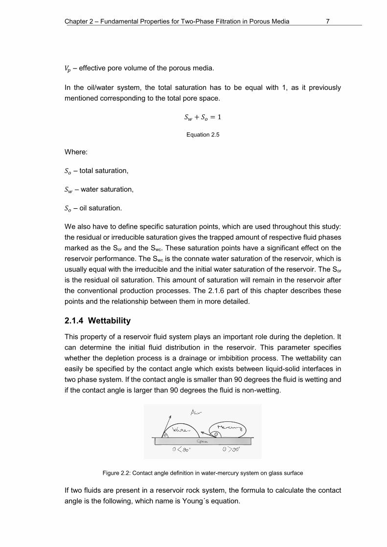
This property of a reservoir fluid system plays an important role during the depletion. It can determine the initial fluid distribution in the reservoir. This parameter specifies whether the depletion process is a drainage or imbibition process. The wettability can easily be specified by the contact angle which exists between liquid-solid interfaces in two phase system. If the contact angle is smaller than 90 degrees the fluid is wetting and if the contact angle is larger than 90 degrees the fluid is non-wetting.
Figure 2.2: Contact angle definition in water-mercury system on glass surface
If two fluids are present in a reservoir rock system, the formula to calculate the contact angle is the following, which name is Young´s equation.

Chapter 2 – Fundamental Properties for Two-Phase Filtration in Porous Media 8
cos 𝜃 =𝜎𝑠2 − 𝜎𝑠1𝜎12
Equation 2.6
Where:
𝜃 – contact angle,
𝜎12 – the interfacial tension between the Fluid 1 and Fluid 2
𝜎𝑠1 – the interfacial tension between the solid surface and the Fluid 1,
𝜎𝑠2 – the interfacial tension between the solid surface and the Fluid 2,
as can be seen in the following schematic picture.
Figure 2.3: Schematic figure of wetting and non-wetting fluids
2.1.5 Permeability (absolute permeability)
The permeability is the resistance to the fluid flow. This concept is defined in 1933 at the first World Oil Congress by Francher, Lewis and Barnes. The name of the unit of the permeability is called Darcy after Henry P. Darcy because the permeability calculation is coming from the above mentioned Darcy`s basic conception.
Figure 2.4: Schematic figure of the Darcy´s law

Chapter 2 – Fundamental Properties for Two-Phase Filtration in Porous Media 9
The final formula called Darcy`s law, which is a strong starting point in the reservoir engineering. This hypothesis describes the flux along an L long tube respect to the ∆𝑝 pressure difference.
Darcy´s law is
𝑞 = −𝐴𝑘
𝜇∇𝑝 = 𝐴
𝑘
𝜇
∆𝑝
𝐿
Equation 2.7
the Darcy velocity can be write as
𝑣 =𝑞
𝐴= −
𝑘
𝜇∇𝑝
Equation 2.8
the formula of the real velocity is
𝑣𝑟𝑒𝑎𝑙 = 𝑣/𝜙 =𝑞
𝐴𝜙= −
𝑘
𝜇𝜙∇𝑝
Equation 2.9
Where:
𝑞 – volumetric flow rate,
𝐴 – cross-sectional area,
𝑘 – permeability of the rock,
𝜇 – viscosity of the fluid,
∇𝑝 – pressure gradient along the core.
𝑣 – Darcy velocity,
𝑣𝑟𝑒𝑎𝑙 – real velocity of the fluid,
𝜙 – porosity of the core.

Chapter 2 – Fundamental Properties for Two-Phase Filtration in Porous Media 10
Darcy units:
[𝑐𝑚3
𝑠] =
[𝑐𝑚2][𝐷]
[𝑐𝑝]
[𝑎𝑡𝑚]
[𝑐𝑚]
SI units:
[𝑚3
𝑠] =
[𝑚2][𝑚2]
[𝑃𝑎. 𝑠]
𝑃𝑎]
[𝑚]
After Darcy the unit of the permeability is Darcy which is equal with m2. If the permeability is the same in every direction the core model is isotropic.
2.1.6 Relative permeability and extended Darcy´s law
Two phase system means that second liquid phase exists in the rock. In the two phase fluid flow system the second fluid means the reduction of cross-section of single phase fluid system.
The relative permeability is a dimensionless factor, which describes the different phases influence on each other under multiphase flow conditions. Speaking about the relative permeability makes sense just in case if two fluid are present in the system at the same time. The relative permeability describes the relative flow behaviour of the phases compared to the absolute permeability, when two fluids are present at the same time in one porous media. The relative permeability is a ratio between effective permeability and the absolute permeability of the rock, as can be seen in the following formula.
𝑘𝑟𝑖 =𝑘𝑖(𝑆𝑖)
𝑘𝑎
Equation 2.10
Where:
𝑘𝑟𝑖 – the relative permeability of phase I,
𝑘𝑖(𝑆𝑖) – the effective permeability of phase I,
𝑘𝑎 – the absolute permeability of the rock.
Basically the sum of the relative permeability will be less than one and the effective permeability should be less than the absolute permeability, because of the capillary pressure and the fluids mutual resistance to each other. On the other hand, regarding to another theory, the relative permeability can be higher than one. Just in case when the
Chapter 2 – Fundamental Properties for Two-Phase Filtration in Porous Media 11
wetting fluid reached the irreducible saturation value and plugged the micro-pores and the other fluid can flow through the rock easier than if just one phase were present. [6]
The extended formula of the Darcy´s law is written for the multiphase filtration. Buckley and Leverett introduced this extension. Buckley-Leverett solution is related to the unsteady state special core measurement calculations, therefore the detailed description of this technique can be seen in the Chapter 2.
𝑞𝑤 = −𝐴𝑘𝑘𝑟𝑤𝜇𝑤
∆𝑝
𝐿
Equation 2.11
𝑞𝑛𝑤 = −𝐴𝑘𝑘𝑟𝑛𝑤𝜇𝑛𝑤
∆𝑝
𝐿
Equation 2.12
Where:
𝑞 – volumetric fluid rate,
𝐴 – cross-sectional area,
𝑘 – absolute permeability of the rock,
𝑘𝑟 – relative permeability of the rock,
𝜇 – viscosity of the fluid,
∆𝑝 – pressure difference,
𝐿 – Length of the core,
w subscript – parameters for the wetting phase,
nw subscript – parameters of the non-wetting phase.
Several relative permeability correlations are proposed, such as Burdin method, LET correlation, and Corey. These correlations can describe the shape of the relative permeability curves if we show them as a function of saturation. In this thesis the most commonly used Corey correlation has been applied.
The following two equations are considered as the general equations for wetting and non-wetting phase base on Corey relation.

Chapter 2 – Fundamental Properties for Two-Phase Filtration in Porous Media 12
𝑘𝑟𝑤 = 𝑘𝑟𝑤𝑛 ∙ (𝑆𝑤𝑒𝑓𝑓)𝑛𝑤= 𝑘𝑟𝑤𝑛 ∙ (
𝑆𝑤 − 𝑆𝑤𝑐1 − 𝑆𝑛𝑤𝑟 − 𝑆𝑤𝑐
)𝑛𝑤
Equation 2.13
𝑘𝑟𝑛𝑤 = (1 − 𝑆𝑤𝑒𝑓𝑓)𝑛𝑛𝑤 = 𝑘𝑟𝑛𝑤𝑛 ∙ (
1 − 𝑆𝑤 − 𝑆𝑛𝑤𝑟1 − 𝑆𝑛𝑤𝑟 − 𝑆𝑤𝑐
)𝑛𝑛𝑤
Equation 2.14
Where:
𝑆𝑤 – given saturation of the wetting phase
(𝑆𝑤𝑒𝑓𝑓) – effective saturation of the wetting phase
𝑘𝑟𝑤(𝑆𝑤) – relative permeability of the wetting phase at the given saturation,
𝑘𝑟𝑛𝑤(𝑆𝑤) – relative permeability of the non-wetting phase at the given saturation
𝑘𝑟𝑤𝑛 – end point of the wetting phase relative permeability curve,
𝑘𝑟𝑛𝑤𝑛 – end point of the non-wetting phase relative permeability curve,
𝑆𝑤𝑐 – connate saturation of the wetting phase,
𝑆𝑛𝑤𝑟 – residual saturation of the non-wetting phase,
𝑛𝑤 – Corey’s exponent of the wetting phase,
𝑛𝑛𝑤 – Corey’s exponent of the non-wetting phase.
The Corey approach can be written for oil and water system in a water wet reservoir rock, as a form of the following equations:
𝑘𝑟𝑤(𝑆𝑤) = 𝑘𝑟𝑤𝑛 ∙ (𝑆𝑤𝑒𝑓𝑓)𝑛𝑤 = 𝑘𝑟𝑤𝑛 ∙ (
𝑆𝑤 − 𝑆𝑤𝑐1 − 𝑆𝑜𝑟 − 𝑆𝑤𝑐
)𝑛𝑤
Equation 2.15
𝑘𝑟𝑜(𝑆𝑤) = 𝑘𝑟𝑜𝑛 ∙ (1 − 𝑆𝑤𝑒𝑓𝑓)𝑛𝑛𝑤 = 𝑘𝑟𝑜𝑛 ∙ (
1 − 𝑆𝑤 − 𝑆𝑜𝑟1 − 𝑆𝑜𝑟 − 𝑆𝑤𝑐
)𝑛𝑛𝑤
Equation 2.16

Chapter 2 – Fundamental Properties for Two-Phase Filtration in Porous Media 13
Where:
𝑆𝑤 – given saturation of the water phase,
(𝑆𝑤𝑒𝑓𝑓) – effective saturation of the water phase,
𝑘𝑟𝑤(𝑆𝑤) – relative permeability of the water phase at the given saturation,
𝑘𝑟𝑜(𝑆𝑤) – relative permeability of the oil phase at the given saturation
𝑘𝑟𝑤𝑛 – end point of the water phase relative permeability curve,
𝑘𝑟𝑜𝑛 – end point of the oil phase relative permeability curve,
𝑆𝑤𝑐 – connate water saturation,
𝑆𝑜𝑟 – residual oil saturation,
𝑛𝑤 – Corey´s exponent of the water phase,
𝑛𝑜 – Corey´s exponent of the oil phase.

Chapter 2 – Fundamental Properties for Two-Phase Filtration in Porous Media 14
Figure 2.5: Typical relative permeability curves of oil and water in water-wet system
The 2.5. Figure shows typical relative permeability curves in a water wet system, if the oil and water are present. If the system is water wet, the cross section point of the relative permeability curves are above 50 % of water saturation. The other points on the relative permeability curves which have significant effect on the flow behaviour in the reservoir are the Swc, Sor krwn, kron, and the exponents nw, no. These parameters are enough to describe the relative permeability curves. Theoretically, the Swc refers to the unmovable water saturation, therefore it can be attached to the kron, which is the end point of the oil relative permeability curve, where the oil relative permeability can reach the highest value.
On the other hand this is the starting point of the water relative permeability curve. Increasing the Sw continuously, the oil relative permeability is decreasing and the water relative permeability is increasing respectively.
Before the water relative permeability curve reaches the highest point and the oil relative permeability curve the lowest point, the cross section point has to be highlighted. The cross section point is very interesting, because at different phase saturations can be the same relative permeability of the phases, furthermore in this point the system has the lowest total mobility value.

Chapter 2 – Fundamental Properties for Two-Phase Filtration in Porous Media 15
The total mobility is coming from summarizing the oil and the water mobility at the same water saturation, because the mobility is saturation dependent.
The phase mobility can be described by the ratio of the phase relative permeability at a given saturation and the dynamic viscosity of the phase, as can be seen below in the 2.16 equation:
𝜆𝑡(𝑆𝑤) = 𝜆𝑤(𝑆𝑤) + 𝜆𝑜(𝑆𝑤) =𝑘𝑟𝑤(𝑆𝑤)
µ𝑤+𝑘𝑟𝑜(𝑆𝑤)
µ𝑜
Equation 2.17
Where:
𝜆𝑡(𝑆𝑤) – total mobility of the system at given water saturation,
𝜆𝑤(𝑆𝑤) – mobility of the water at given water saturation,
𝜆𝑜(𝑆𝑤) – mobility of the oil at given water saturation,
𝑘𝑟𝑤(𝑆𝑤) – relative permeability of the water at given water saturation
µ𝑤 – viscosity of the water,
𝑘𝑟𝑜(𝑆𝑤) – relative permeability of the oil at given water saturation
µ𝑜 – viscosity of the oil.
Finally with increasing the water saturation, the water curve reaches the maximum value of the relative permeability which is the end point saturation of the water relative permeability curve. This maximum water saturation is equal to the 1-Sor, when the oil relative permeability curve reaches its minimum.
The Sor is theoretically that saturation of the oil phase when the oil becomes immobile, therefore the kro is zero, just the water can flow in the system, and the oil is present just in unmovable/irreducible form.
The last values are the two exponent of the oil and water curves. These values are responsible for the shape of the curves. In case of ni = 1 the curve is linear and if the exponent is increasing, the curve has bigger curvature. In the industry practice, the typical exponents of the oil and water system is between 2 and 4 in case of water wet system. The typical relative permeability values can be seen in the Reservoir Simulation I. Lecture Notes [2].
Chapter 2 – Fundamental Properties for Two-Phase Filtration in Porous Media 16
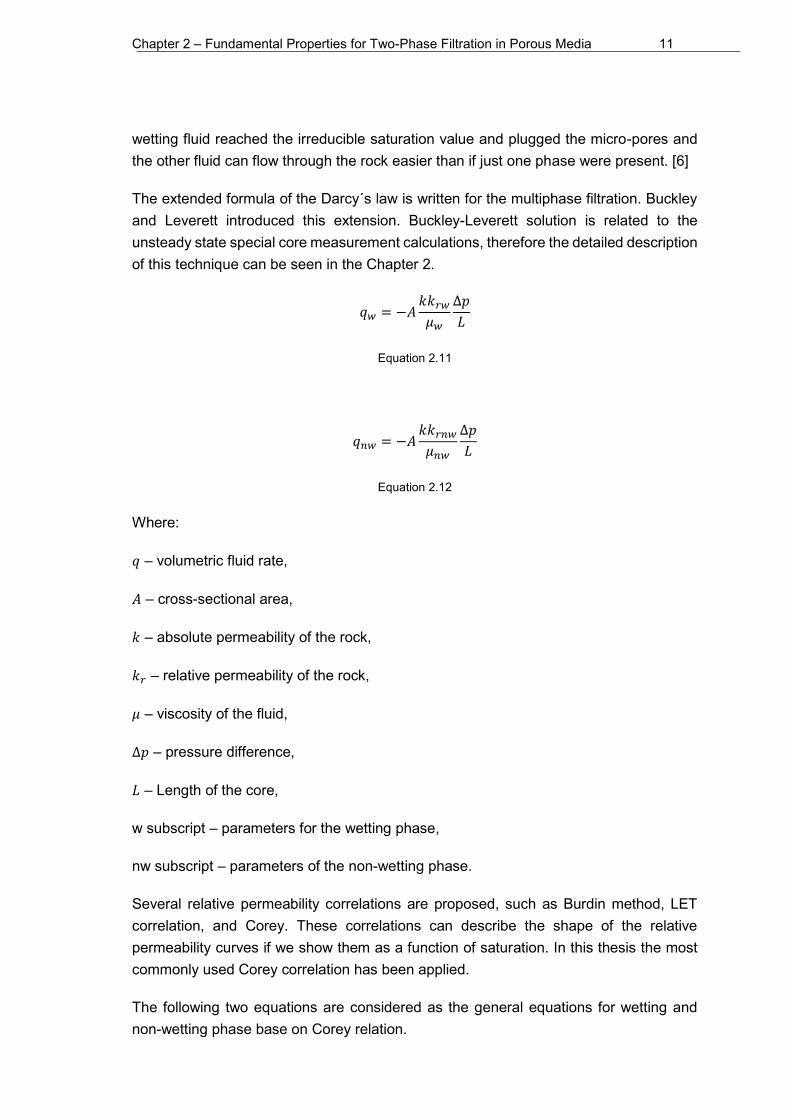
2.1.7 Wettability effect on the relative permeability
Figure 2.6: Typical relative permeability curves based on wettability [2]
We can differentiate the rock according to the wettability:
water-wet, oil-wet, intermediate-wet, mixed wet.
In an intermediate wet rock system the wettability cannot be defined accurately, because the discrepancy between the physical properties of the present fluids are insignificant. In case of a mixed wet rock system oil- and water wet regions vary along the reservoir.
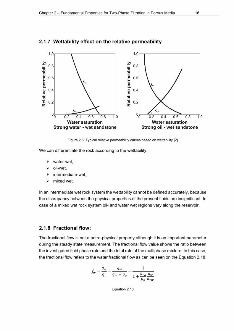
2.1.8 Fractional flow:
The fractional flow is not a petro-physical property although it is an important parameter during the steady state measurement. The fractional flow value shows the ratio between the investigated fluid phase rate and the total rate of the multiphase mixture. In this case, the fractional flow refers to the water fractional flow as can be seen on the Equation 2.18.
𝑓𝑤 =𝑞𝑤𝑞𝑡=
𝑞𝑤𝑞𝑤 + 𝑞𝑜
=1
1 +𝑘𝑟𝑜𝜇𝑜
𝜇𝑤𝑘𝑟𝑤
Equation 2.18

Chapter 2 – Fundamental Properties for Two-Phase Filtration in Porous Media 17
Where:
𝑓𝑤 – water fractional flow,
𝑞𝑤 – water rate,
𝑞𝑜 – oil rate,
𝑞𝑡 – total rate.
Figure 2.7: Typical fractional flow curve [8]

Chapter 2 – Fundamental Properties for Two-Phase Filtration in Porous Media 18
2.2 Fluid properties Beside the petro-physical properties, the other required quantities are the fluid properties. In a reservoir different fluids are present in different phases. During this study the fluids are considered as immiscible fluids. These phases have an inter-phase; therefore the interfacial tension has to be introduced. The phases have different basic properties such as density, which causes the pressure difference between them, called capillary pressure. The description of these quantities and parameters can be found below.
2.2.1 Density under surface conditions
The density is an essential parameter of the fluid phases, because it indicates another parameter, which has an important effect on the reservoir behaviour, this is the capillary pressure. The density of the fluid can be expressed as how many kg of this material exists in 1 m3 volume. This quantity depends on the pressure and the temperature. The equation can be seen below.
𝜌𝑖(𝑝, 𝑇) =𝑚𝑖
𝑉𝑖
Equation 2.19
Where:
𝜌𝑖(𝑝, 𝑇) – density of the fluid of “i”,
𝑚𝑖 – mass of the fluid “i”,
𝑉𝑖 – volume of the fluid “i”.
2.2.2 Formation volume factor
The formation volume factor is an important parameter of the fluids in the reservoir.
It shows the ratio between the volumes of the fluid phase “i” at reservoir conditions and the volume of the fluid phase “i” at surface conditions. We can define the formation volume factor with the following equation.
𝐵𝑖 =𝑉𝑖(𝑝𝑟𝑒𝑠, 𝑇𝑟𝑒𝑠)
𝑉𝑖(𝑝𝑠𝑐 , 𝑇𝑠𝑐)
Equation 2.20

Chapter 2 – Fundamental Properties for Two-Phase Filtration in Porous Media 19
Where:
𝐵𝑖 – formation volume factor of the fluid phase “i”,
𝑉𝑖(𝑝𝑟𝑒𝑠, 𝑇𝑟𝑒𝑠) – volume of the fluid phase “i” at reservoir conditions,
𝑉𝑖(𝑝𝑠𝑐 , 𝑇𝑠𝑐) – volume of the fluid phase “i” at surface conditions.
2.2.3 Fluid compressibility – isothermal compressibility
The isothermal fluid compressibility is describing the fluid volume changes respect to the pressure changes at constant temperature.
𝐶𝑓 = −1
𝑉𝑓(𝜕𝑉𝑓
𝜕𝑝)𝑇
Equation 2.21
Where:
𝐶𝑓 – fluid compressibility,
𝑉𝑓 – fluid volume,
(𝜕𝑉𝑓
𝜕𝑝)𝑇 – derivative of fluid volume with respect to pressure at constant temperature
During this study, the incompressible fluid flow assumption implies this parameter is equal to zero. The reason is the pressure difference along the core during the experiments are relatively low to count with this effect. The complexity of model will not increase significantly the accuracy of the final result.
2.2.4 Viscosity - µ
The viscosity describes the resistance of the fluid against the flow. We can differentiate two types of viscosity, one of them is the dynamic viscosity, and other one is the kinematic viscosity. The dynamic viscosity is describing the fluid deformation in presence of any shear stress.
𝜏 = 𝜇𝜕𝜑
𝜕𝑡
Equation 2.22
Where:
𝜏 – Shear stress,

Chapter 2 – Fundamental Properties for Two-Phase Filtration in Porous Media 20
𝜇 – Dynamic viscosity,
𝜕𝜑
𝜕𝑡 – angular velocity.
The kinematic viscosity is expressed by the dynamic viscosity divided by the fluid density.
𝑣 =𝜇
𝜌
Equation 2.23
Where:
𝑣 – Kinematic viscosity,
𝜇 – Dynamic viscosity,
𝜌 – density of the fluid.
2.2.5 Capillary pressure
The capillary force comes from the pressure difference between the present fluids in a porous media. The pressure difference is coming from the previously mentioned quantity, which was the density. Each fluid phase has different density.
𝑃𝑐 = 𝑝𝑛𝑤 − 𝑝𝑤
Equation 2.24
Where:
𝑃𝑐 – Capillary pressure,
𝑝𝑛𝑤 – The hydrostatic pressure of the non-wetting phase,
𝑝𝑤 –the hydrostatic pressure of the wetting phase.
If the equilibrium has been assumed on the interface of the two phase the capillary pressure can be the function of the geometry, on the micro scale, as can be seen in the Young Laplace equation.
𝑃𝑐 =4𝜎12 cos𝜃
𝑑=2𝜎12 cos 𝜃
𝑟
Equation 2.25
Chapter 2 – Fundamental Properties for Two-Phase Filtration in Porous Media 21
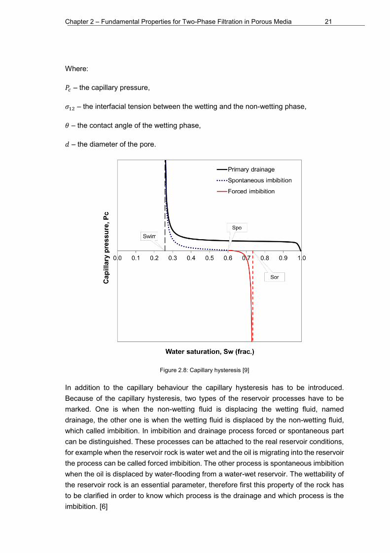
Where:
𝑃𝑐 – the capillary pressure,
𝜎12 – the interfacial tension between the wetting and the non-wetting phase,
𝜃 – the contact angle of the wetting phase,
𝑑 – the diameter of the pore.
Figure 2.8: Capillary hysteresis [9]
In addition to the capillary behaviour the capillary hysteresis has to be introduced. Because of the capillary hysteresis, two types of the reservoir processes have to be marked. One is when the non-wetting fluid is displacing the wetting fluid, named drainage, the other one is when the wetting fluid is displaced by the non-wetting fluid, which called imbibition. In imbibition and drainage process forced or spontaneous part can be distinguished. These processes can be attached to the real reservoir conditions, for example when the reservoir rock is water wet and the oil is migrating into the reservoir the process can be called forced imbibition. The other process is spontaneous imbibition when the oil is displaced by water-flooding from a water-wet reservoir. The wettability of the reservoir rock is an essential parameter, therefore first this property of the rock has to be clarified in order to know which process is the drainage and which process is the imbibition. [6]

Chapter 2 – Fundamental Properties for Two-Phase Filtration in Porous Media 22
The following schematic Figure 2.9 demonstrates the relationship between the remarkable saturation points.
Figure 2.9: Schematic figure of the capillary hysteresis in a water wet system, Curve: 1: drainage (water displaced by oil), Curve 2: imbibition (oil displaced by water)
When the reservoir is at initial stage, the production starts from the end of the first curve which is the starting point of the second imbibition curve, at the Swc saturation value. The initial phase distribution can easily be determined in the reservoir by the primary drainage capillary curve as can be seen on the Figure 2.10.
Figure 2.10: Equilibrium between gravity and capillary forces [2]

Chapter 3 – SCAL measurements – Common Techniques 23
3 SCAL measurements – Common Techniques In the chapter, experimental techniques are discussed that are related to the models developed in the frame of this thesis. Other SCAL techniques are ignored.
3.1 Two phase relative permeability Relative permeability has been investigated for a long time. Physical and empirical models are applied to gain information about these saturation functions. The most common amongst those can be classified into four categories. These categories are capillary-bundle models, pore network models and empirical representations.
Capillary-bundle models: The capillary-bundle models are based on viscous flow in capillaries as can be described by law found by Hagen and Poiseuille. The porous medium is composed of a bundle of capillaries. A statistical distribution of capillary diameters can be introduced to adapt the model to different rock types. Furthermore, an arbitrary cross sectional shape and tortuosity can be introduced. However, the capillaries are not interconnected and hence the model is just of limited use to describe realistic rock properties.
Pore network models: Pore network models use the network connections between pore bodies and throats often derived from real rocks to model the porous media. These are paying attention on the pathways, the connections and the complexity of the porous system.
Empirical models: Empirical models are generalized models to parametrize saturation functions to describe experimental data. The empirically determined general relative permeability curves, therefore these can provides the most realistic results.
Many factors can affect the two phase relative permeability, but not all of these effects are not significant or independent. Historically, the following factors have been investigated as described in detailed in [5]: saturation states, structural properties of the rock, wettability, effective stress, porosity and permeability, temperature, interfacial tension, density, viscosity, initial wetting phase saturation, the presence of a third phase.
In the meantime, the number of significant parameters could be reduced to parameters modifying capillary pressure like exact pore geometry, interfacial tension and wettability.
The relative permeability of rock for each fluid phase can be measured in a core sample by either steady state or unsteady-state techniques, such as SS and USS relative permeability or USS centrifuge methods that will be explained in the following.
Chapter 3 – SCAL measurements – Common Techniques 24
3.2 Steady-State Method Many techniques can be differentiated in steady state method, the common experiments are the Penn-State, Single Sample Dynamic, Stationary Fluid, Hassler, Hafford and Dispersed Feed Method [5]. Numerous techniques have been successfully employed to obtain a uniform saturation. The primary concern about designing the experiment is to eliminate or reduce saturation gradients, which is caused by capillary pressure effects at the outflow boundary of the core. This is called “the capillary end effect”.
In this thesis we refer to steady state method modified the one first proposed by Hassler in 1944. In the original Hassler method semipermeable membranes (either permeable to oil or to water) are installed, these membranes can separate the two fluid phases from each other at the inlet and the outlet and allow the two fluids to flow through the core simultaneously. Since the fluid phases are separated at the inlet and outlet, the individual fluid phase pressure can be measured. The original Hassler technique provides very uniform saturation values along the whole core length.
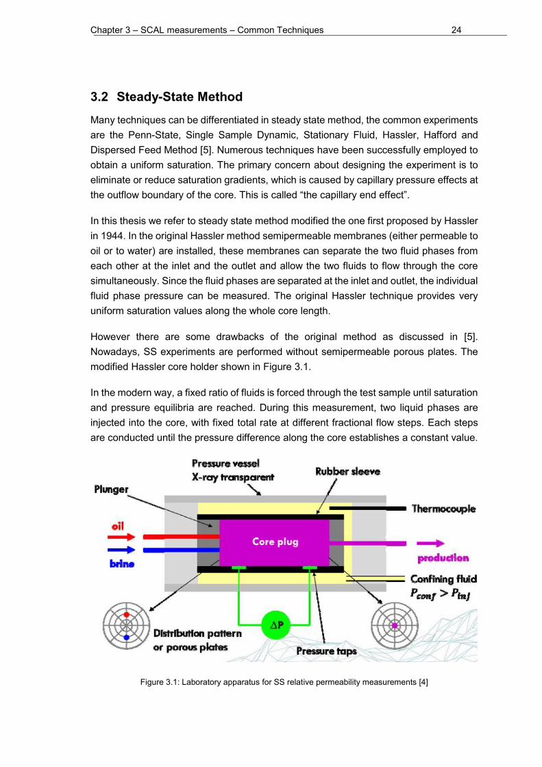
However there are some drawbacks of the original method as discussed in [5]. Nowadays, SS experiments are performed without semipermeable porous plates. The modified Hassler core holder shown in Figure 3.1.
In the modern way, a fixed ratio of fluids is forced through the test sample until saturation and pressure equilibria are reached. During this measurement, two liquid phases are injected into the core, with fixed total rate at different fractional flow steps. Each steps are conducted until the pressure difference along the core establishes a constant value.
Figure 3.1: Laboratory apparatus for SS relative permeability measurements [4]

Chapter 3 – SCAL measurements – Common Techniques 25
From the provided data, which are injection rate, fractional flow steps, pressure difference and the saturation profile, the relative permeability values for each fractional flow step and the two phases can be calculated easily by the extended Darcy`s law, which is described in Chapter 2.
Steady-state methods are preferred over unsteady-state methods, because generally a higher saturation range can be investigated and it is the officially accepted standard to measure relieve permeability, because data are used for reserve calculations of companies and states.
3.3 Unsteady-State Method Another class of methods that are frequently used investigate relative permeability under unsteady state conditions, which means that the measure variables are time dependent. USS relative permeability can be measured in the laboratory under ambient (slightly elevated P and T condition) or (more rarely) under simulated reservoir conditions. USS measurements are typically much faster to perform, but have some shortcomings compared to the steady state method. The first important limit is that the core has to be homogeneous. The second is to keep the driving force and the fluid properties constant. In addition the pressure gradient has to be large enough to neglect the capillary pressure effects. Regarding to the compressibility effects, we can handle the compressibility as an insignificant parameter related to the pressure difference compare the operated pressure. These assumptions for experiment design are important to make a reliable test for interpret the results.
Several analysis techniques have been proposed to derive the relative permeability from unsteady-state core floods. The most commonly applied is the JBN method based on Buckley-Leverett theory as also applied in this thesis.
The unsteady-state relative permeability measurements is simpler than the steady-state one. The unsteady state experiment has a main advantage and disadvantage: This core test is very quick compare to the steady state one. We compare a few hours in case if USS to a few weeks for the SS method. The main deficit is coming from the analytical model, which implies some complexity in combination with crude assumptions. The mathematical approach which is used for interpretation of the unsteady-state experimental results is the Buckley –Leverett theory extended by Welge. [5]
𝑓𝑤2 =1 +
𝑘𝑜𝑞𝑡𝜇𝑜
∙ (𝜕𝑃𝑐𝜕𝑥
− 𝑔∆𝜌 sin𝜃)
1 +𝑘𝑜𝑘𝑤
∙𝜇𝑤𝜇𝑜
Equation 3.1

Chapter 3 – SCAL measurements – Common Techniques 26
Where:
𝑓𝑤2 – the fraction of the water at outlet stream,
𝑞𝑡 – the velocity of total fluid leaving the core,
𝜃 – the angle between horizontal and direction x,
∆𝜌 – the density difference between the displacing and displaced fluids.
Welge assumed the capillary pressure is zero, and that case when the flow is horizontal, the previous equation means we can write the following Equation 3.2.
𝑆𝑤,𝑎𝑣 − 𝑆𝑤2 = 𝑓𝑜2𝑄𝑤
Equation 3.2
𝑆𝑤,𝑎𝑣 – the average water saturation,
𝑆𝑤2 – the water saturation at the outlet,
𝑓𝑜2 – the fraction of the oil at the outlet stream
𝑄𝑤 – the injected cumulative water.
We can measure the amount of the injected cumulative water and the average water saturation at the outlet stream experimentally.
From these values we can easily determine the fraction of the oil phase at the outlet side by graphical method. When the Qw and Sw,av plot, and the slope can give the fo2, with the following definition of the fractional flow.
𝑓𝑜2 = 𝑞𝑜/(𝑞𝑜 + 𝑞𝑤)
Equation 3.3
When we combining it with the Darcy definition we can get the following relationship for fractional flow and between the mobility of the phases:
𝑓𝑜2 =1
1 +𝜇𝑜/𝑘𝑟𝑜𝜇𝑤/𝑘𝑟𝑤

Chapter 3 – SCAL measurements – Common Techniques 27
Equation 3.4
The viscosity of each phases are known, therefore we can easily determine the ratio between the relative permeability of the phases.
The theory behind the JBN function [1] is the same to calculate the relative permeability for each phase from USS measurement. The deference is in the deduction and the final form of the equation as can be seen below.
𝑘𝑟𝑜 =𝑓𝑜2
𝑑 (1
𝑄𝑤𝐼𝑟) /𝑑 (
1𝑄𝑤)
Equation 3.5
𝑘𝑟𝑤 =𝑓𝑤2𝑓𝑜2
𝜇𝑤𝜇𝑜𝑘𝑟𝑜
Equation 3.6
Where the new introduced variable is the Ir which is the ratio between the injectivity and the initial injectivity. The injectivity means that the water rate at the injected stream is divided by the pressure difference along the core. USS techniques are now employed for most laboratory measurements of relative permeability. The derivation of the Buckley Leverett solution can be find out at [8]

Chapter 3 – SCAL measurements – Common Techniques 28
3.4 Centrifuge Methods This Centrifuge technique has been widely used to derive capillary pressure saturation functions and partly to obtain information about relative permeability. For relative permeability, the centrifuge method is much faster than the SS. The centrifuge method is can be used to predict the capillary end effect. In general, the centrifuge techniques involves monitoring liquid produced from the core.
The rock sample is initially saturated with one or two phases. The liquids are collected in a transparent tube connected to a rock sample holders. With the stroboscopic lights and a CCD detector, the fluid level of the produced fluid in the rotating tubes can be monitored. The schematic figure of the centrifuge apparatus can be seen on the 3.2. Figure.
Figure 3.2: Automated centrifuge system at imbibition and drainage setup [4]
Two different setups exist in centrifuge method covering drainage and imbibition processes.
In the centrifuge measurement, the key parameter is the centrifugal acceleration; it can be calculated from the rotation speed of the tube. Two types of centrifuge measurement can be distinguished from each other. One is the single speed centrifuge measurement and the other one is the multispeed centrifuge measurement.
In the single speed, the core is rotating with just one rotational speed. The single speed is used for determination of the relative permeability of the expelled phase, and particularly useful to determine the relative permeability close to the end points, the connate water saturation during the drainage and residual oil saturation during the imbibition. In the multi-speed experiments, the core sample is rotated at steps of increasing speed corresponding to steps on the capillary pressure curve. The multispeed

Chapter 3 – SCAL measurements – Common Techniques 29
experiment is proper to determine the capillary pressure curves. To derive results from centrifuge measurements, different analytical solutions exist, e.g. the Hassler-Brunner method, which is commonly is applied [5]. To extract the relative permeability of the expelled phase in a single-speed measurement, the Hagoort`s method can be applied [5]. The detailed description of these method can be found in the SCAL lecture notes [4].
3.4.1 The Burdine Method to calculate relative permeability
It is possible to calculate relative permeability data from capillary pressure measurements as the first time shown by Purcell and Burdine [10] .The Burdine method is limited because it is valid only in case of drainage, when the wetting-phase is displaced by the non-wetting fluid.
The calculation of the relative permeability using capillary pressure is proposed by Burdine, related to Purcell`s work, as can be seen in Equation 3.7 and Equation 3.8.
𝑘𝑟𝑤(𝑆𝑊) = (𝑆𝑊 − 𝑆𝑤𝑐
1 − 𝑆𝑤𝑐 − 𝑆𝑛𝑤𝑟)2 ∫
𝑑𝑆𝑤𝑃𝑐2⁄
𝑆𝑊𝑆𝑤𝑐
∫𝑑𝑆𝑤
𝑃𝑐2⁄
1−𝑆𝑛𝑤𝑟
𝑆𝑤𝑐
Equation 3.7
𝑘𝑟𝑛𝑤(𝑆𝑊) = (1 − 𝑆𝑊 − 𝑆𝑛𝑤𝑟1 − 𝑆𝑤𝑐 − 𝑆𝑛𝑤𝑟
)2 ∫
𝑑𝑆𝑤𝑃𝑐2⁄
1−𝑆𝑛𝑤𝑟
𝑆𝑊
∫𝑑𝑆𝑤
𝑃𝑐2⁄
1−𝑆𝑛𝑤𝑟
𝑆𝑤𝑐
Equation 3.8
Where:
𝑘𝑟(𝑆𝑊) – relative permeability of the phase wetting or non-wetting at actual saturation,
𝑆𝑊 – actual wetting phase saturation,
𝑆𝑤𝑐 – connate saturation of the wetting phase,
𝑆𝑛𝑤𝑟 – irreducible non-wetting phase saturation,
𝑑𝑆𝑤 – saturation difference,
𝑃𝑐 – capillary pressure.

Chapter 4 – Numerical Methods 30
4 Numerical Methods In this chapter of the thesis the applied simulator should be defined and explained. In addition the used methods and their mathematical background is discussed in this chapter. We focus on the parts necessary for work performed in the thesis.
4.1 The applied simulator: ECLIPSE From the Eclipse family the used simulator for this core simulation the ECLIPSE 100.
Eclipse (Schlumberger Ltd.) – ECLIPSE 100 (black oil simulator)
Eclipse is a software package developed by Schlumberger Ltd. which is a French oil field company founded in 1926. Two simulators are existing in ECLIPSE, which are the following:
E100 (ECLIPSE 100) is a fully implicit integrated finite difference three phase general purposed black oil simulator.
E300 (ECLIPSE 300) is a K-value thermal compositional simulator with cubic equation of states which has temporal discretization approaches of IMPES, FIM and in AIM. The spatial discretization of the governing equation is finite difference method.
4.2 Mathematical background of multiphase flow and transport The steps to reach the final numerical solution are the following:
Formulation of the respective PDE’s, Non-linear PDE`s, Discretization, Non-linear Algebraic Equations, Linearization, Linear Algebraic Equations (LAE), Solution of the LAE.
4.2.1 Discretization methods:
Instead of searching for continuous solution, look for approximated values of the solution on a finite set of grid points at discrete time levels. Requires a grid system with grid points and control volumes.
Differential operators are approximated by difference formulas. Reduces the partial differential equations with boundary conditions to non-linear algebraic equations that can be linearized.

Chapter 4 – Numerical Methods 31
Available methods for discretization:
FDM – Finite Difference Method - The applied method in this work FEM – Finite Element Method CVM – Control Volume Method
4.2.2 Newton-Raphson
The difference equations obtained from the discretization method are not linear. The Newton Rapson method is a linearization method for the equations in the reservoir simulator, because the partial differential equations (PDE`s) are not linear. This method uses the Taylor series to linearize the PDE´s equations.
To solve the linearized equations, two types of solution can be applied, the iterative or the direct solution methods. The iterative solver method is Jacobi iterations for example. The iterative method starting from an initial guess, the iteration is continuously repeating when calculated value reached the given stopping criteria or the iteration maximum. Very good solution for practical problems.
In my thesis, I investigate two phase immiscible flow. The balance equation is given by the conservation of mass (continuity equation) on 4.1 equation and the extended Darcy’s Law, which is a particular solution of Stokes equation on 4.2 equation.
𝜕(𝑆𝑖𝜙𝜌𝑖)
𝜕𝑡+ 𝑑𝑖𝑣(𝜌𝑖𝑣𝑖) − 𝜌𝑖𝑄𝑖 = 0
𝑖 ∈ {𝑤, 𝑛𝑤}
Equation 4.1
Where:
𝑆𝑖 – saturation of the phase “i”,
𝜙 – porosity of the rock,
𝜌𝑖 – density of the phase “i”,
𝑡 – time,
𝑣𝑖 – velocity of the phase “i”,
𝑄𝑖 – source/flux of the phase “i”

Chapter 4 – Numerical Methods 32
𝑣𝑖 = −𝑘𝑟𝑖𝜇𝑖𝐾(∇𝑝𝑖 − 𝜌𝑖�⃗�)
𝑖 ∈ {𝑤, 𝑛𝑤}
Equation 4.2
Where:
𝑘𝑟𝑖 – relative permeabilty of the phase “i”,
𝜇𝑖 – viscosity of the phase “i”,
𝐾 – absolute permeability of the rock,
∇𝑝𝑖 – pressure gradient of the phase “i”,
𝜌𝑖 – density of the phase “i”,
�⃗� – Gravitational acceleration (constant vector).
In this case, the assumptions are incompressible fluid flow and incompressible solid phase, therefore we can write the equations formulated for wetting (water) and non-wetting (oil) phase with the following equations:
𝐿(𝑆𝑤, 𝑣𝑤) ∶= 𝜙𝜕(𝑆𝑤)
𝜕𝑡+ 𝑑𝑖𝑣(𝑣𝑤) − 𝑄𝑤 = 0
Equation 4.3
𝐿(𝑆𝑛𝑤, 𝑣𝑛𝑤) ∶= 𝜙𝜕(𝑆𝑛𝑤)
𝜕𝑡+ 𝑑𝑖𝑣(𝑣𝑛𝑤) − 𝑄𝑛𝑤 = 0
Equation 4.4
4.2.3 Darcy`s law used in Reservoir Simulation
The Darcy`s law in the Reservoir Simulation is used in modified form.
The Darcy`s law can be differentiate into three parts. One is the transmissibility, which is the geometrical factor, the second one is the mobility of the phase, which is a function of rock and PVT properties and the last one is the pressure difference of the phase.

Chapter 4 – Numerical Methods 33
𝑞𝑖 = 𝜏 ∙ 𝜆𝑖 ∙ ∆𝑝𝑖 =𝑘𝑘𝑟𝑖𝐴∆𝑝𝑖𝜇𝑖𝐿
Equation 4.5
𝜏 =𝑘𝐴
𝐿
𝜆𝑖 =𝑘𝑟𝑖𝜇𝑖
Where:
𝜏 – transmissibility,
𝜆𝑖 – mobility of the phase “i”.
In the reservoir simulation, we use implicit and explicit methods to solve the linearized equations. First, I have to introduce two methods, which is able to calculate the pressure and saturation changes during the whole simulation. We can calculate these values with implicit or explicit functions.
Implicit method means the calculation at the given time step does not use the previous time step solution, this method solve the equation at each time step, and then iterate.
The other method is the explicit, which means the calculated value at the given time step is using the previous time step solutions for the iteration.
Three types of numerical calculations are defined in reservoir simulation, which are the combinations of the above described methods, these are IMPES (Implicit Pressure Explicit Saturation), FIM (Fully Implicit Method), AIM (Adaptive Implicit Method)
IMPES method is calculating the pressure implicitly and the saturation explicitly. In the FIM method the simulator calculate the pressure and the saturation as well by implicit solver. In the AIM case the simulator combines the advantages of IMPES and FIM.
In this worked the used simulation method was the fully implicit method, because of the good stability of solution.
4.2.4 Peaceman`s well model
It is important to talk about the well models, because in the SS and USS models, the fluid injection and production defined by wells.

Chapter 4 – Numerical Methods 34
The wells are located at the middle of the grid block. Theoretically the wells are defined as a source term in the fluid flow equations. In the conventional reservoir simulation, when the whole reservoir is simulated the block of the wells are very large compared to the real well bore diameter. This is the reason behind why well models are applied. The well model is translating the block pressure into a bottom hole flowing pressure.
Several well models are available, with different assumptions. The applied well model is the Peaceman`s well model, which describes the relationship between the block pressure, the bottom hole flowing pressure and the production rate.
Assumptions:
two dimensional fluid flow, isolated well, regular grid blocks, uniform blocks.
𝑝𝑤𝑓 = 𝑝𝑜 −𝜇𝑞
2𝜋𝑘ℎ𝑙𝑛𝑟𝑜𝑟𝑤
Equation 4.6
Where:
𝑝𝑤𝑓 – flowing bottom-hole pressure,
𝑝𝑜 – pressure of the grid cell,
𝜇 – viscosity,
𝑞 – volumetric flow rate (positive case is production, negative case is injection),
𝑘 – permeability of the reservoir,
ℎ - height of reservoir,
𝑟𝑜 – equivalent well radius,
𝑟𝑤 – well radius.
In this equation the key parameter is the equivalent well radius. Which has the following meaning: “It is convenient to associate an equivalent well radius, ro, with the well block. This is the radius at which the steady-state flowing pressure for the actual well is equal to the numerically calculated pressure for the well block.” - D.W.Peaceman [2]

Chapter 4 – Numerical Methods 35
4.3 General description of the .data file for Eclipse The data file should include the following sections: RUNSPEC, GRID, EDIT, PROPS, REGIONS, SOLUTION, SUMMARY, SCHEDULE.
RUNSPEC:
This section has to be include the following the title of the file (TITLE), the number of block in X,Y and Z directions(DIMENS), the active phase present, that is which of the saturations (Rs or Rv) vary(OIL,WATER,GAS,VAPOIL,DISGAS), the unit convection (FIELD / METRIC / LAB), the start date of the simulation (START). In ECLIPSE 300 the START keyword is only mandatory if the DATES keyword is used. The last thing should be the well and group dimensions (WELLDIMS).
TITLE DIMENS OIL,WATER,GAS,VAPOIL,DISGAS FIELD / METRIC / LAB START WELLDIMS
GRID:
In this section the first step is the reservoir geometry that has to be defined using keywords CART or RADIAL. If we use a block centred Cartesian grid, the essential keywords are the following:
DXV DYV DZ TOPS PORO PERMX PERMY PERMZ
EDIT:
The EDIT section is entirely optional. The edit section contains the modifying block centre depths, pore volumes, transmissibility, diffusivities (for the Molecular Diffusion option), and non-neighbour connections (NNCs) computed by the program from the data entered in the grid section.

Chapter 4 – Numerical Methods 36
PROPS:
The props section is used to define the PVT and SCAL data. Tables of properties of reservoir rock and fluids as functions of fluid pressures, saturations and compositions (density, viscosity, relative permeability, capillary pressure, etc.). Contains the equation of state description in compositional runs.
REGIONS:
Splits computational grid into regions for calculation of:
PVT properties (fluid densities and viscosities) Saturation properties (relative permeability and capillary pressures) Initial conditions (equilibrium pressures and saturations) Fluids in place (fluid-in-place and inter-region flows) EoS regions (for compositional runs)
If this section is omitted, all grid blocks are put in region 1
SOLUTION:
Specification of initial conditions in reservoir. May be:
Calculated using specified fluid contact depths to give potential equilibrium Read from a restart file setup by an earlier run Specified by the user for every grid block
(not recommended for general use)
RESTART file:
SUMMARY:
Specification of data to be written to the Summary file after each time step. Necessary if certain types of graphical output (for example water-cut as a function of time) are to be generated after the run has finished. If this section is not written no Summary files are created, therefore the results cannot be visualized directly.
SCHEDULE
The schedule section is used to define the operating conditions of the reservoir over time. It includes the specification of well and perforation histories. Historical production and pressure measurements. Specifies the operations to be simulated (production and injection controls and constraints) and the times at which output reports are required.

Chapter 4 – Numerical Methods 37
Vertical flow performance curves and simulator tuning parameters may also be specified in the SCHEDULE section.
Detailed description of the keywords can be found in ECLIPSE Reference Manual. [11]

Chapter 5 – Models setup 38
5 Models setup In history matching, before we start simulation, the system has to be in equilibrium. This process is called initialization. In the typical history matching process on a field simulation the initial equilibrium requires that the gravitational forces have to be equal with the capillary forces at each point in the reservoir. In the initialization method we have to define the initial pressure distribution and the phase distribution in the reservoir. It should be defined with pressure gradients of the phases, calculated by reference depth. The initial saturation distribution can be determined with the primary drainage capillary pressure curves, as it was written in detailed in the Chapter 2.
But in the core simulation the initial system is well defined by a single pressure. For the initial saturation we just have to give the connate saturation of the wetting fluid and the rest is filled with the non-wetting fluid.
The initialization is correct when these two requirements are completed – pressure and saturation equilibration. Both requirements are satisfied if there is no fluid movement in the system.
5.1 Boundary and initial conditions These models are homogenous pseudo 1D, because they have x, y and z coordinate. The boundary conditions are not the same in the investigated cases, therefore these specific conditions are described in case of every models. The only common point is the no flow boundary assumed over all boundaries of the model domain: at the top, at the bottom and on the sides as well. Flow and production has been modelled by introducing wells – for details see below.
5.2 Steady state model The forward simulation keywords of the SS model can be seen in the Appendix A.
Grid:
The built mesh is a simple pseudo-1D realization with one layer of cells in y and z direction. In horizontal direction the resolution is chosen to be high using 50 cells, with addition cells at both ends of the domain in which the wells are placed. The system results in 50 × 1 × 1 mesh. The grid is schematically displayed in Figure 5.1, which shows the SS core model from top view. The colour code represents the porosity, which has been chosen to be homogeneous, except of the boundary cells. The reason behind the two cells at both ends are different is that they do not belong to the rock domain and should not contribute to the pressure drop.

Chapter 5 – Models setup 39
Figure 5.1: Schematic figure of the SS core model in above view
Fluids:
The system is built for two phase systems. One is the aqueous phase and the other one is the oleic phase.
Initialization:
The initial state of the model, before injection starts, represents the initial experimental condition in the core. Which means the set pressure is constant and actual experimental pressure experiments are typically performed starting at connate water saturation, which is used as the initial saturation state of all experiments analysed in the frame of this thesis.
Simulator control:
The applied simulator control was set at a constant injection rate, with a defined fractional flow schedule. The observed data is the pressure difference at the injection well and the water saturation profile along the core sample. The production pressure (experimental back pressure) was held constant at each time step.
Wells:
The fluid injection in and production from in the core is simulated by wells. For the constant rate simulations, one injection well has been defined, and for the constant outlet pressure one production well has been defined.
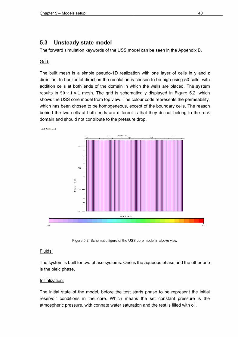
Chapter 5 – Models setup 40
5.3 Unsteady state model The forward simulation keywords of the USS model can be seen in the Appendix B.
Grid:
The built mesh is a simple pseudo-1D realization with one layer of cells in y and z direction. In horizontal direction the resolution is chosen to be high using 50 cells, with addition cells at both ends of the domain in which the wells are placed. The system results in 50 × 1 × 1 mesh. The grid is schematically displayed in Figure 5.2, which shows the USS core model from top view. The colour code represents the permeability, which has been chosen to be homogeneous, except of the boundary cells. The reason behind the two cells at both ends are different is that they do not belong to the rock domain and should not contribute to the pressure drop.
Figure 5.2: Schematic figure of the USS core model in above view
Fluids:
The system is built for two phase systems. One is the aqueous phase and the other one is the oleic phase.
Initialization:
The initial state of the model, before the test starts phase to be represent the initial reservoir conditions in the core. Which means the set constant pressure is the atmospheric pressure, with connate water saturation and the rest is filled with oil.

Chapter 5 – Models setup 41
Simulator control:
The applied simulator control was constant injection rate, which is just water rate. The observed data is the pressure difference at the injection well and the average water saturation changes during the simulation. The production pressure should be constant at each time step.
Wells:
The fluid injection in and production from in the core is simulated by wells. For the constant rate one injection well defined, and for the constant outlet pressure one production well is defined.
5.4 Centrifuge model
For this type of experiments, the model setup is almost completely different than the previously discussed SS and USS simulation models. Two types of centrifugal measurement can be differentiated, one is the single speed experiment, and the other one is the multispeed. During the single speed, the core is rotated with just one speed until the equilibrium is reached. During the multispeed test, the rotation speed is changed stepwise after the respective equilibrium state has been reached and the measurements has been taken. In both type of centrifuge experiment, two method can be differentiated based on the type of expelled fluid phase, corresponding to imbibition and drainage.
Grid:
During investigation, different representations of the model has been worked out until a satisfactory performance and numerical stability could be reached. Only the stable case is presented here. The centrifuge model is build up in vertical direction to introduce gravity and is pseudo-2D geometry to allow for horizontal invasion mimicking the experimental geometry. In vertical direction – the main flow direction – the model was assigned a high resolution of 50 cells, with addition cells on the sides, and on the top of the core has an addition part, which has the same length as the core. This upper part represents the collection tube. The size of the side-wall cells are chosen to be 10 percent of the central cells, as earlier described in [DR].
The system results in 3 × 1 × 100 mesh. The schematic figure of the grid shown in Figure 5.3.

Chapter 5 – Models setup 42
Figure 5.3: Schematic figure of the Centrifuge core model in front view with initial saturations
Fluids:
The system is built for two phase systems. One is the aqueous phase and the other one is the oleic phase. Since we have incompressible fluids the density appears only in gravity term. Therefore we just applied different PVT tables with different densities for each layer, where the fluid density is calculated as a function of gravity, function of relative distance from the centre of the core.
Initialization:
The initial state of the model, before the test starts phase to be represent the initial reservoir conditions in the core. The fluid distribution is depends on the process types of the measurements, imbibition or drainage. The only difference between the imbibition and drainage is the place of the collection tube, but the gravity has not been flipped, the gravity always points downwards. The history matched case as shown in the result section is performed in imbibition. In case of multispeed scenarios, for each applied rotation speed a new simulation has to be started from previously saved simulation results in RESTART file. In all of the multispeed scenarios, for each experimentally applied rotational speed a new gravity acceleration is applied for simulation.

Chapter 5 – Models setup 43
Simulator control:
The applied simulator control was the gravitational acceleration changes. In each grid block a different gravity constant has been applied to simulate the dependence of acceleration from the distance to the rotational axis. This setup was given with the gravity is not constant, the gravity is different in each location (each grid blocks). The variation of the gravity constant was calculated from the rotational speed through centrifugal accelerations.
The observed data are average saturation changes during the simulation and cumulative production data.
Due to the specific setup of the centrifuge methods, during experiment and simulation, there is no injection and production to and from the experimental/simulation domain. This is the reason why the simulator control is intrinsic to the model, which is described in Chapter 3. Because we do not inject anything into the core, we just use the centrifugal acceleration to separate the fluids in the modelling domain or core holder, respectively. Eclipse cannot simulate rotational movements. Therefore the simulation is like a gravitational segregation.
The gravity constant s calculated from the angular velocity by [9]:
𝑔 = 𝜔2𝑟 = (2𝜋𝑅𝑃𝑀
60)2
𝑟
Equation 5.1
Where:
𝑔 – gravitational acceleration,
𝜔 – angular velocity,
𝑟 – radius
RPM – rotation speed.
Wells:
No wells. The fluid flow is not simulated by injection in and production from in the core. The monitoring technique for “oil production” made by “ROFT” keyword which shows how much oil flow out of the core.

Chapter 6 – Benchmark – Validation 44
6 Benchmark – Validation The chapter is describing the validation method. The benchmark is necessary for the analysis of experimental data, we need a correct numerical model of the experimental domain. SCAL models are not common modules in ECLIPSE. Therefore, the freshly build models need to be verified and benchmarked against standards before they can be used for history matching of experimental data, because if the validity of the models are not proven, we never know these models are correct or not.
The benchmarking involves running simulation test cases, that could be either process or site related. The aim of this benchmark is to determine the validity of the constructed model in ECLIPSE. This benchmark is just a model validation, software performance benchmark, without any changes.
Benchmarking has been done against four different simulation tools as used earlier for analysing experiments [11]. For this, forward simulations of fictive experiments performed with the four simulation tools have been compared. The results shows that the here developed models compare to a high degree to standards, which validates the approach, as shown in the following sections of the chapter. For validation, 5 datasets and simulation results were used from SCA2016-006 paper [12]. The purpose of this SCA paper was to be a well-documented reference case to verification other simulator core models.
The four simulators are: CYDAR, PORLAB, SCORES, SENDRA
For all simulator, fife cases corresponding to 5 models were performed as forward simulations. The cases are the following:
Case 1 - Steady-state imbibition with a smooth Pc curve: Water and oil injected at increasing water fractional flow, followed by several bump floods.
Case 2 - Steady-state imbibition with a sharp Pc curve: Same as Case 1 with sharper curve.
Case 3 - Unsteady-state imbibition with a smooth Pc curve: Only water injected with increasing flow rates.
Case 4 - Unsteady- state imbibition without Pc curve (Buckley Leverett): Only water injected with only one flow rate with capillary pressure neglected.
Case 5 - Primary Drainage centrifuge: Analytical case where the local and average Pc curves are well known.
The compared results are shown below, but detailed description and core properties can be found in [12].

Chapter 6 – Benchmark – Validation 45
6.1 1st case results In the first case, the tested model was the steady-state imbibition core model with smooth Pc curve. The simulated process is water and oil injection with increasing water fractional flow, followed by two bump-floods. The following figures show the comparison of SCORES (DuMuX) and ECLIPSE simulation results.
Figure 6.1 shows the calculated differential pressure along the core at each fractional flow step. Figure 6.2 shows the calculated cumulative oil production. Figure 6.3 shows calculated average water saturation.
Figure 6.1: Case 1 – Calculated differential pressure in SS measurement with smooth Pc curve
0.0
0.5
1.0
1.5
2.0
2.5
3.0
3.5
4.0
0.0 2.5 5.0 7.5 10.0 12.5 15.0 17.5 20.0 22.5
Dif
fere
nti
al p
ress
ure
[b
ar]
Time [hour]
Differential pessure [bar]
DuMuX
Eclipse
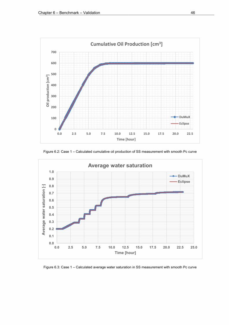
Chapter 6 – Benchmark – Validation 46
Figure 6.2: Case 1 – Calculated cumulative oil production of SS measurement with smooth Pc curve
Figure 6.3: Case 1 – Calculated average water saturation in SS measurement with smooth Pc curve
0
100
200
300
400
500
600
700
0.0 2.5 5.0 7.5 10.0 12.5 15.0 17.5 20.0 22.5
Oil
pro
du
ctio
n [
cm3 ]
Time [hour]
Cumulative Oil Production [cm3]
DuMuX
Eclipse
0.0
0.1
0.2
0.3
0.4
0.5
0.6
0.7
0.8
0.9
1.0
0.0 2.5 5.0 7.5 10.0 12.5 15.0 17.5 20.0 22.5 25.0
Aver
age
wat
er s
atur
atio
n [-]
Time [hour]
Average water saturation
DuMuXEclipse

Chapter 6 – Benchmark – Validation 47
6.2 2nd case results In 2nd case, the process is the same with the 1st case, the difference is just the capillary pressure curve. The tested model was the steady-state imbibition core model with sharp Pc curve. The simulated process is water and oil injection with increasing water fractional flow steps, followed by several bump-floods. The following figures show the comparison of SCORES (DuMuX) and ECLIPSE simulation results.
Figure 6.4 shows the calculated differential pressure along the core at each fractional flow step. Figure 6.3 shows the calculated cumulative oil production. Figure 6.6 shows calculated average water saturation.
Figure 6.4: Case 2 – Calculated differential pressure in SS measurement with smooth Pc curve
0.0
0.5
1.0
1.5
2.0
2.5
3.0
3.5
4.0
0.0 2.5 5.0 7.5 10.0 12.5 15.0 17.5 20.0 22.5
dif
fere
nti
al p
ress
ure
[b
ar]
Time [hour]
Differential pessure [bar]
DuMuX
Eclipse
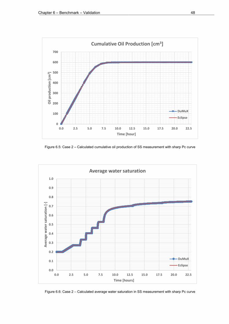
Chapter 6 – Benchmark – Validation 48
Figure 6.5: Case 2 – Calculated cumulative oil production of SS measurement with sharp Pc curve
Figure 6.6: Case 2 – Calculated average water saturation in SS measurement with sharp Pc curve
0
100
200
300
400
500
600
700
0.0 2.5 5.0 7.5 10.0 12.5 15.0 17.5 20.0 22.5
Oil
pro
du
ctio
n [
cm3 ]
Time [hour]
Cumulative Oil Production [cm3]
DuMuX
Eclipse
0.0
0.1
0.2
0.3
0.4
0.5
0.6
0.7
0.8
0.9
1.0
0.0 2.5 5.0 7.5 10.0 12.5 15.0 17.5 20.0 22.5
Ave
rage
wat
er
satu
rati
on
[-]
Time [hours]
Average water saturation
DuMuX
Eclipse

Chapter 6 – Benchmark – Validation 49
6.3 3rd case results In 3rd case, the tested model is the unsteady-state imbibition model with smooth Pc curve. The simulated process is only water injection with increasing water flow rate. The following figures show the comparison of SCORES (DuMuX) and ECLIPSE simulation results.
Figure 6.7 shows the calculated differential pressure along the core. Figure 6.8 shows the calculated cumulative oil production. Figure 6.9 shows calculated average water saturation.
Figure 6.7: Case 3 – Calculated differential pressure in USS measurement with smooth Pc curve
0.0
0.5
1.0
1.5
2.0
2.5
3.0
3.5
4.0
0.0 2.5 5.0 7.5 10.0 12.5 15.0 17.5 20.0 22.5 25.0
Dif
fere
nti
al p
ress
ure
[b
ar]
Time [hour]
Differential pessure [bar]
DuMuX
Eclipse

Chapter 6 – Benchmark – Validation 50
Figure 6.8: Case 3 –– Calculated cumulative oil production of USS measurement with smooth Pc curve
Figure 6.9: Case 3 – Calculated average water saturation in USS measurement with smooth Pc curve
0
2
4
6
8
10
12
14
0.0 2.5 5.0 7.5 10.0 12.5 15.0 17.5 20.0 22.5 25.0
Oil
pro
du
ctio
n [
cm3 ]
Time [hour]
Cumulative Oil Production [cm3]
DuMuX
Eclipse
0.0
0.1
0.2
0.3
0.4
0.5
0.6
0.7
0.8
0.9
1.0
0.0 2.5 5.0 7.5 10.0 12.5 15.0 17.5 20.0 22.5 25.0
Ave
rage
wat
er
satu
rati
on
[-]
Time [hour]
Average water saturation
DuMuX
Eclipse

Chapter 6 – Benchmark – Validation 51
6.4 4th case results In 4th case, the tested model is the unsteady-state imbibition model without Pc curve. The simulated process is only water injection with single water flow rate. The following figures show the comparison of SCORES (DuMuX) and ECLIPSE simulation results.
Figure 6.10 shows the calculated differential pressure along the core. Figure 6.11 shows the calculated cumulative oil production. Figure 6.12 shows calculated average water saturation.
Figure 6.10 Case 4 – Calculated differential pressure in USS measurement without Pc curve
Figure 6.11: Case 4 – Calculated cumulative oil production of USS measurement without Pc curve
0.5
0.7
0.9
1.1
1.3
1.5
1.7
0.0 0.1 0.2 0.3 0.4 0.5 0.6 0.7 0.8 0.9 1.0 1.1
Dif
fere
nti
al p
ress
ure
[b
ar]
Time [hour]
Differential pessure [bar]
DuMuX
Eclipse
0
2
4
6
8
10
12
14
0.0 0.1 0.2 0.3 0.4 0.5 0.6 0.7 0.8 0.9 1.0 1.1
Oil
pro
du
ctio
n [
cm3 ]
Time [hour]
Cumulative Oil Production [cm3]
DuMuX
Eclipse

Chapter 6 – Benchmark – Validation 52
Figure 6.12: Case 4 – Calculated average water saturation in USS measurement without Pc curve
6.5 5th case results In 5th case, the tested model is the primary drainage centrifuge mode. The simulated process is only the analytical case, where the local and average Pc curves are well known. The following pictures show the comparison of the valid core simulator results and my ECLIPSE core model results.
Figure 6.13 shows the calculated cumulative oil production. Figure 6.14 shows calculated average water saturation.
0.1
0.2
0.3
0.4
0.5
0.6
0.7
0.8
0.0 0.1 0.2 0.3 0.4 0.5 0.6 0.7 0.8 0.9 1.0 1.1
Ave
rage
wat
er
satu
rati
on
[-]
Time [hour]
Average water saturation
DuMuX
Eclipse

Chapter 6 – Benchmark – Validation 53
Figure 6.13: Case 5 – Calculated cumulative water production of centrifuge measurement
Figure 6.14: Case 5 – Calculated average water saturation of centrifuge measurement
0.0
2.5
5.0
7.5
10.0
12.5
15.0
17.5
20.0
22.5
25.0
0.0 2.5 5.0 7.5 10.0 12.5 15.0 17.5 20.0 22.5 25.0 27.5 30.0
Wat
er
pro
du
ctio
n [
cm3 ]
Time [hour]
Cumulative water production [cm3]
DuMuX
Eclipse
0.0
0.1
0.2
0.3
0.4
0.5
0.6
0.7
0.8
0.9
1.0
0.0 2.5 5.0 7.5 10.0 12.5 15.0 17.5 20.0 22.5 25.0 27.5 30.0
Ave
rage
wat
er
satu
rati
on
[-]
Time [hour]
Average water saturation
DuMuX
Eclipse
Chapter 7 – History matching (HM) 54
7 History matching (HM) History matching process is an ill-posed inverse problem. It is trial and error process, because the objective of the history matching is to minimize the mismatch between simulated and observed data by adjusting certain model parameters. Such process almost never has a unique solution. [2]
7.1 Basic Concept of History Matching: The basic concept of the History Matching consists of adjusting parameters of the built simulation model until when the simulated data is in good agreement with historical data. In conventional history matching common observed data are water-cut, GOR, average reservoir pressure (static, shut-in pressure), flowing well pressure, oil rates, and breakthrough time and so on.
The inverse modelling approach means that the input parameters are unknown. The purpose of HM is to find the best set of input data to reproduce the historically observed data. Inverse problem almost never has a unique solution. The reason why it cannot give unique solution is many different sets of input data can reproduce the same performance.
The quality of the history matching does not just dependent on the matching quality. The uncertainty of the history matching result can come also from the validity and the quality of dynamical input data, such as measured production history data.
The history matching is time consuming, it takes a large portion of a reservoir study and usually history matching is made by hand. In conventional history matching, usually it happens in two phases, first to match globally observed data, secondly to match locally observed data.
The rule of thumb suggests to first change that parameter which has the biggest influence on the simulated result and which has the highest uncertainty. In conventional history matching to change the relative permeability data is the last resort, because it has very significant effect on the simulated data, therefore it has to be defined accurately before history matching process [13].
7.1.1 Differences between conventional history matching (CHM) and SCAL history matching (SHM)
The only differences between conventional history matching and core history matching are the scales and the complexity of the models.
The scale of the model in case of conventional history matching is always field scale, in case of SCAL history matching is always core-scale (macro). The second important difference is the conditions. During the conventional field simulation the history matching

Chapter 7 – History matching (HM) 55
process is working at reservoir conditions, while the SCAL model is working at reservoir or laboratory conditions.
Last but not least the third huge difference is the complexity of the models. In a field simulation there can be several hundred of wells and the models are heterogeneous and anisotropic. In SCAL history matching, there are only two wells, injection and production well. The amount of observation data is smaller than in CHM. The SHM model is still homogenous and one dimensional. The goal of the CHM is to match the observed and the calculated data in good agreement, such as shape at the end of the history. The following step is to make prediction for future, the forecast of the production data will start from the last part of the history, therefore that can acceptable if just the shape and end part of the dataset are in good agreement. In general it means, during the history matching procedure, several weighted option can be used related to the given parameters and the purpose of the matching.
There are experimental results from relative permeability measurements. These data are coming from laboratory interpretation applying analytical methods. As previously described, these analytical methods have simplified assumptions which give inaccurate results and errors such as the capillary end effect and the interaction of capillary and viscous forces during the steady-state (SS) and unsteady-state (USS) calculations or the space variations of centrifugal acceleration during centrifuge (C) data interpretation.
In ideal case if we had proper relative permeability, it would match with the measured data. In eclipse end points, residual oil and connate water saturation can be matched, but not possible to find an automated match for Corey exponents. Therefore a Python script has been created in order to make an appropriate history matching tool, which suits for SCAL history matching.
After this SHM process, the matched kr and Pc curves can be used as a fixed input data in CHM model. The SHM can be defined as a pre-process of the CHM, which decreases the uncertainty of the CHM.
7.2 External software – Python The reason behind to use Python script is the deficiencies of the ECLIPSE, which are coming from the software itself. The limitation has been found during the development of the SS, USS and C model.
Figure 7.1 shows the workflow of the model SCAL Assisted History Matching (AHM) tool contraction process.

Chapter 7 – History matching (HM) 56
Figure 7.1: Steps of the core model development
The ECLIPSE has a history matching tool, namely SimOpt. Tabulated kr and Pc curves can be matched via SimOpt, but with certain limitations, because none of well know parametrizations with corresponding industrial analogies for kr and Pc cannot be used internally by ECLIPSE.
Naturally, the tabulated dataset can be generated by hand based on related functions. Therefore, the history matching of the measurements can be made by hand. Matching the kr and Pc manually is too time consuming and it is not so flexible. In case of an own laboratory where all of the measured data could be matched, it is more efficient to use an automatic matching tool.
On the other hand, the SimOpt tool is working with only end-point scaling, the tabulated kr curves can have limited matching. End-point scaling means to change the kr curves` end points to give a wider or thicker range to the kr curves. End-point scaling is a good starting point to reach a good match, but the Corey exponents of the curves (Co, Cw) are not negligible. Otherwise, if just one core flooding experiment exists and the centrifuge imbibition measurement is not available, the residual oil saturation (Sor) should be an addition matching parameter.
The previously mentioned deficiencies mean that the existing history matching tool of the ECLIPSE cannot be applicable for SCAL data history matching. Furthermore, it is considered as inappropriate tool for matching laboratory measurements results.
The purpose of this work is to make general models, which can be matched automatically for every type of SCAL experiments.

Chapter 7 – History matching (HM) 57
7.2.1 What does Python do?
The Python script does an automated history matching process with ECLIPSE running in the background to produce a forward simulation. At each optimization step the new ECLIPSE project is generated automatically by python based on current guess of model parameters. The results from ECLIPSE are later used to calculate the objective function of respective optimization problem.
7.2.2 Generating kr and Pc curves
The relative permeability and capillary pressure curves are adapted in ECLIPSE simulation by generation of corresponding input files in form of saturation function tables. Python applies Corey function for the relative permeability curves, which can be seen in the Equation 7.1 and Extended Corey correlation for the capillary pressure curves which can be seen in the Equation 7.2.
Corey correlation for kr curves:
𝑘𝑟𝑤(𝑆𝑤) = 𝑘𝑟𝑤𝑒𝑛𝑑 ∙ (
𝑆𝑤 − 𝑆𝑤𝑐1 − 𝑆𝑤𝑐 − 𝑆𝑜𝑟
)𝑛𝑤
𝑘𝑟𝑜(𝑆𝑤) = 𝑘𝑟𝑜𝑒𝑛𝑑 ∙ (
1 − 𝑆𝑤 − 𝑆𝑜𝑟1 − 𝑆𝑤𝑐 − 𝑆𝑜𝑟
)𝑛𝑜
Equation 7.1
Extended Corey correlation for Pc curves:
𝑃𝑐 =
{
𝐴𝑤 ∙ (1 −
𝑆𝑤 − 𝑆𝑤𝑐𝑆𝑤𝑑 − 𝑆𝑤𝑐
)𝑐𝑤
+ 𝑆𝑤𝑑 ∙ 𝑟𝑖 + 𝑏𝑖
𝑆𝑤 ∙ 𝑟𝑖 + 𝑏𝑖
𝐴𝑜 ∙ (1 −1 − 𝑆𝑤 − 𝑆𝑜𝑟1 − 𝑆𝑜𝑑 − 𝑆𝑜𝑟
)𝑐𝑜
+ 𝑆𝑜𝑑 ∙ 𝑟𝑖 + 𝑏𝑖
Equation 7.2
Assumptions:
𝑆𝑤𝑐 ≤ 𝑆𝑤 < 𝑆𝑤𝑑
𝑆𝑤𝑑 ≤ 𝑆𝑤 ≤ 𝑆𝑜𝑑
𝑆𝑜𝑑 < 𝑆𝑤 ≤ 1 − 𝑆𝑜𝑟

Chapter 7 – History matching (HM) 58
Where:
𝐴𝑤 , 𝐴𝑜 – height of curve pc area near water and oil zone correspondingly
𝑟𝑖 – slope of linear part (Plato)
𝑆𝑤: 𝑆𝑤𝑐 < 𝑆𝑤𝑑 < 𝑆𝑜𝑑 < 1 − 𝑆𝑜𝑟
Figure 7.2 Remarkable point of the Extended Corey function on capillary pressure curve
The generated parameter combinations can be controlled, the ranges for each matching parameters have to be specified by user. Therefore, the tool can be called assisted history matching tool, because it is automated and controlled.
7.2.3 History matching algorithm
The next step in the Python script is the history matching algorithm after the input files generation. The goal of the automated history matching algorithm is to choose the best match between observed and simulated data by minimizing the objective function. Most of the history matching tools are using optimization approaches which can be separated in two big groups. One of each is stochastic approaches like EnKF and ErML. [14]. Another big group is gradient approaches.

Chapter 7 – History matching (HM) 59
To our interest the objective function in the following form is going to be considered:
𝐽(𝑈, 𝛼) =
= 𝑊𝑝 ∙ ∑ 𝑤𝑝𝑖 ∙ (∆𝑝𝑖
𝑜𝑏𝑠𝑟𝑣 − ∆𝑝𝑖𝑐𝑎𝑙𝑐
𝜎∆𝑝)
2𝑁(𝑜𝑏𝑠𝑟𝑣)
𝑖=1
+𝑊𝑄 ∙ ∑ 𝑤𝑄𝑖 ∙ (𝑄𝑖𝑜𝑏𝑠𝑟𝑣 − 𝑄𝑖
𝑐𝑎𝑙𝑐
𝜎𝑄)
2
+
𝑁(𝑜𝑏𝑠𝑟𝑣)
𝑖=1
+𝑊𝑆̅ ∑ 𝑤�̅�𝑖 ∙ (𝑆�̅�𝑜𝑏𝑠𝑟𝑣 − 𝑆�̅�
𝑐𝑎𝑙𝑐
𝜎�̅�)
2𝑁(𝑜𝑏𝑠𝑟𝑣)
𝑖=1
Equation 7.3
Where:
𝐽(𝑈) –objective function,
𝑊 – weighting factor of the observation data respect to the superscript,
𝑤 – weighting factor of the observation at each value respect to the superscript,
∆𝑝 – differential pressure,
𝑄 – cumulative liquid production,
𝑆̅ – average saturation of water.
Superscripts:
𝑝 – pressure,
𝑄 – cumulative liquid production,
𝑆 – water saturation,
𝑖 = 1… 𝑁(𝑜𝑏𝑠𝑟𝑣) – number of observation data,
𝑜𝑏𝑠𝑟𝑣 – observation data from measurements,
𝑐𝑎𝑙𝑐 – calculated data value by simulation.
The applied weighting factors are Wp = 2500, WQ = 25, WS = 400. The higher value of the weighting factor represents the bigger importance of related property during the matching.
The Gradient Optimization approach has been used in this work to find the minimum value for the objective function. To achieve that the derivatives of objective function with respect to the model parameters such as Corey exponents, kr end points, capillary entry

Chapter 7 – History matching (HM) 60
pressure, residual oil saturation, connate water saturation has to be calculated. Different methods exist to calculate the derivative of objective function:
Direct approach Adjoint approach Finite difference approach
In our optimization algorithm the finite different approach was used:
𝑑𝐽
𝑑�⃗�= [
𝐽(𝑈, �⃗� + 𝜀∆�⃗�) − 𝐽(𝑈, �⃗� − 𝜀∆�⃗�)
2𝜀]
𝑇
�⃗� = [𝛼𝑖 …𝛼𝑁]𝑇
Equation 7.4
Where:
𝑑𝐽
𝑑�⃗⃗⃗� – derivative of objective function with respect to model parameters (gradient of
objective function),
�⃗� – vector of model parameters,
𝛼𝑖 – individual component of model parameters,
𝑈 – primary variables of two phase flow model (pressure, saturation, injection rates).
Based on the calculation of gradient the direction in which the parameter space should be modified in order to minimize the objective function can be defined.
For good initial estimation of model parameters as the first approximation the analytical solution was used and then the brute force and Nelder-Mead algorithms were applied to improve it. For more accurate calculation the gradient approach L-BFGS-B (Broyden-Fletcher-Goldfarb-Shanno algorithm) is applied at the end.
Brute force optimization approach:
In this study the Brute force optimization approach was the first applied optimization algorithm, which is very simple. This is like a trial and error approach. Practically it is generating ECLIPSE simulation runs with all possible parameter combinations from a given set of values (given values within certain ranges generated by applied increments).

Chapter 7 – History matching (HM) 61
Nelder-Mead optimization approach:
Secondly, the applied method was the Nelder-Mead optimization algorithm after the brute force. It is a generalized bi-section (DICHOTOMY) unconstraint optimization approach, for high dimensional parameter spaces. This algorithm is robust and it does not require any Hessian matrix calculation and it is applicable for wide range of functions.
L-BFGS-B (Broyden-Fletcher-Goldfarb-Shanno algorithm) – gradient optimization approach:
Finally, the gradient approach was applied. It is a quasi-Newton method, because it uses approximated Hessian matrix from provided gradient of the function of interest (objective function). At any next iteration, the vector of parameters is changed according to new step and direction. It uses line search procedure to find an appropriate step by bi-section approach. This is the most accurate algorithm from the applied ones with ability to set up constraints. [15]

Chapter 7 – History matching (HM) 62
7.3 Results of the matched (improved) data from the SS, USS, C experiments
The relative permeability curves can cover in wide saturation range with SCAL experiments. The covered part are well shown on the Figure 7.3: The covered part of the relative permeability curves by each SCAL experiment
Figure 7.3: The covered part of the relative permeability curves by each SCAL experiment [9]
This picture shows the SS can cover a widest range of the relative permeability curves from all of the SCAL experiments. The USS experiment can cover a smaller range than SS.
The Centrifuge measurement covers the vicinity of residual oil saturation because it extended the relative permeability curve in higher water saturation direction. This part is not reachable any other above mentioned experiments.
7.3.1 Matching Steady-State data
The real dataset has been found for history matching by using the SS model as described before. The dataset is available in a SPE publication, which described the workflow to test the predictive capability of pore scale modelling [7]. The used fluid and rock dataset is summarized in the following Table 7.1.
The oil permeability measurement has been done under reservoir conditions, in presence of initialized connate water saturation.

Chapter 7 – History matching (HM) 63
Table 7.1: Fluid and rock properties of SS imbibition measurement; taken from [7].
Fluid and rock properties
Data unit
L 5 cm
d 3.76 cm
K 4.9 mD
φ 0.268 -
Swc 0.06 -
Sor 0.13 -
µw 0.000426 Pa.s
µo 0.001053 Pa.s
ρw 1.108 g/cm3
ρo 0.782 g/cm3
The simulator control data were the injection rates and the respective fractional flow values. The injection schedule was defined in ten fractional flow steps, with a given constant total injection rate, as summarized in Table 7.2. With the first eight steps almost the whole saturation range between Swc and 1-Sor was covered (fractional flow steps: 0.01, 0.05, 0.15, 0.50, 0.85, 0.95, 0.99, 1) with constant 30 cc/hour injection rate. At the end of the steady state experiment a last flooding step was performed as a so called bump flood, with relatively high injection rate. The reason to apply bump floods is to come closer to Sor and to decrease the capillary end effect with increased flow rate.
Table 7.2: Injection schedule for Steady State measurement
Schedule for SS
Injection period
Time Qtotal fw qo/qt qw/qt
[hour] [cc/s] [-] [%] [%]
1 0 30 0.01 99 1
2 50.4 30 0.05 95 5
3 71.9 30 0.15 85 15
4 97.2 30 0.5 50 50
5 121 30 0.85 15 85
6 146 30 0.95 5 95
7 168 30 0.99 1 99
8 193 30 1 0 100
9 219 200 1 0 100
10 239 500 1 0 100

Chapter 7 – History matching (HM) 64
The observation data from this measurement are the pressure difference along the core and saturation profiles obtained by X-ray shadowgraphs. In addition, capillary pressure values are available from centrifuge measurement, but unfortunately the centrifuge raw data has not been available. All of the observation data has been matched and are in good agreement. However, between the analytical and numerical interpretations there are some significant differences, as can be seen in the following 7.3.1.1 and 7.3.2.2 part.
7.3.1.1 Observation and Simulated data
The analytically interpreted relative permeability was used at first for a forward simulation. The Figure 7.4 and Figure 7.5 show the simulated results of the first forward simulation. There is no matching point in both. The observed data do not fit together with the numerical calculation. Therefore, we have to match the relative permeability curve, to fit the calculated data to history data of the measurement.
Figure 7.4: SS Measured (blue symbols) and simulated (red line) pressure drops at various fractional flow steps.
0
1
2
3
4
5
6
7
8
9
0 25 50 75 100 125 150 175 200 225 250
Pre
ssu
re [
bar
]
Time [hours]
SS: Measured and Simulated Pressure Difference
observed calculated

Chapter 7 – History matching (HM) 65
Figure 7.5: SS Measured (symbols) and simulated (line) water saturation profiles at various fractional flow steps
The following pictures show the best calculated results of the controlled history matching process.
The most sensitive data is the pressure difference along core for each fractional flow step. The injection during each fractional flow step goes until the pressure difference reached a constant value, which means that steady state flow has been reached and the system is in dynamic equilibrium. Another necessary condition for reaching equilibrium is a stable saturation profile along the core.
The match between simulation and observed data is in a reasonably good agreement. As can be seen in Figure 7.6 the differential pressure shows little mismatch in the begging and in end of the experiment (high and low fractional flow steps) i.e. near to the residual saturations. A reason is could be that the shape of the relative permeability curve differs from Corey closer to the end points. Therefore it is recommended to try other type parameterization such as LET [16].
-0.09
0.01
0.11
0.21
0.31
0.41
0.51
0.61
0.71
0.81
0.91
0 0.5 1 1.5 2 2.5 3 3.5 4 4.5 5
Sw [
frac
tio
n]
Core length [cm]
SS: Water Saturation Profiles
Sw1 Sw2 Sw3 Sw4 Sw5
Sw6 Sw7 Sw8 Sw9 Sw10
Sw1 calc Sw2 calc Sw3 calc Sw4 calc Sw5 calc
Sw6 calc Sw7 calc Sw8 calc Sw9 calc Sw10 calc

Chapter 7 – History matching (HM) 66
Figure 7.6: SS Measured (blue symbols) and simulated (red line) pressure drops at various fractional flow steps.
Figure 7.7: SS Measured (symbols) and simulated (line) water saturation profiles at various fractional flow steps
0
0.5
1
1.5
2
2.5
3
3.5
4
4.5
5
0 25 50 75 100 125 150 175 200 225 250
Pre
ssu
re [
bar
]
Time [hours]
SS: Measured and Simulated Pressure Difference
observed calculated
0
0.1
0.2
0.3
0.4
0.5
0.6
0.7
0.8
0.9
1
0 0.5 1 1.5 2 2.5 3 3.5 4 4.5 5
Sw [
frac
tio
n]
Core length [cm]
SS: Water Saturation Profiles
Sw1 Sw2 Sw3 Sw4 Sw5Sw6 Sw7 Sw8 Sw9 Sw10Sw1 calc Sw2 calc Sw3 calc Sw4 calc Sw5 calcSw6 calc Sw7 calc Sw8 calc Sw9 calc Sw10 calc

Chapter 7 – History matching (HM) 67
As can be seen in the Figure 7.7 and Figure 7.8 the water saturation increases with each step. The match of the saturation profiles shows a mismatch in the last two stages, but otherwise is acceptable considering the match of other observables.
Figure 7.8: SS Measured (green symbols) and simulated (blue line) average water saturation at various fractional flow steps.
Figure 7.9: SS Simulated cumulative oil production
Figure 7.9 shows the reproduced production curve. Generally the cumulative liquid production is measured and available, but not given in the publication [7].
0
0.1
0.2
0.3
0.4
0.5
0.6
0.7
0.8
0.9
1
0 25 50 75 100 125 150 175 200 225 250
Sw a
vera
ge [
frac
tio
n]
Time [hour]
SS: Average Water Saturation
observed calculated
0
500
1000
1500
2000
2500
3000
3500
0 25 50 75 100 125 150 175 200 225 250
Cu
mu
lati
ve O
il P
rod
uct
ion
[cm
3]
Time [hour]
SS: Cumulative Oil Production [cm3]

Chapter 7 – History matching (HM) 68
7.3.1.2 Matched Parameters
In this part, the measured and simulated relative permeability curves can be seen.
Figure 7.10: SS analytical calculated (symbols) and simulated (lines) relative permeability values at various fractional flow steps in linear and logarithmic scale
Figure 7.10 shows the mismatch between the analytical and numerical evaluations of the SS data set. The numerical approach as described before takes capillary pressure and hence the capillary end effect into account. We therefore believe in the quality of the numerical simulation compared to the analytical solution. However, the data set as presented here, still shows some deviations especially in relation to the bump flood that tells us probably the capillary pressure interpretation should be improved numerically.
The best case would be to simultaneously match two experiments, steady-state and centrifuge (raw data from both experiments and combined simulation model are needed).
The calculated Corey parameters by numerical simulation shown in Table 7.3.
It is important to calculate accurately, because in sense of field simulation these difference can cause huge mistake in production forecast.
0
0.1
0.2
0.3
0.4
0.5
0.6
0.7
0.8
0.9
1
0 0.2 0.4 0.6 0.8 1
kr [
frac
tio
n]
Sw [fraction]
SS: Measured versus Simulated Relative
Permeability Curves
kro(analytical) krw(analytical)
krw(matched) kro(matched)
0.000001
0.00001
0.0001
0.001
0.01
0.1
1
0 0.5 1
kr [
frac
tio
n]
Sw [fraction]
SS: Measured versus Simulated Relative
Permeability Curves (log-scale)
kro(analytical) krw(analytical)
krw(matched) kro(matched)

Chapter 7 – History matching (HM) 69
Figure 7.11: Centrifuge Measured (symbols) and SS simulated (lines) capillary pressure values at various fractional flow steps.
The input capillary pressure curve was originally derived from centrifuge experiment is displayed in Figure 7.11 and has been taken as given (raw data were not available). Since there was no possibility to check the quality of this measurement, because from any measurement to recalculate the interpreted values without raw data is impossible.
Otherwise the simulation gave a good match without change the capillary pressure curve.
Table 7.3: SS Simulated Corey parameters of Relative Permeability
SS: Simulated Relative permeability
- Water Oil
Residual saturation 0.06 0.13
End point 0.7 1.0
Corey exponent 3.36 3.25
-2
-1.5
-1
-0.5
0
0.5
1
1.5
2
0 0.2 0.4 0.6 0.8 1Pc
[bar
]
Sw [fraction]
Capillary pressure

Chapter 7 – History matching (HM) 70
7.3.2 Matching Un-Steady-State data
In case of unsteady-state model an artificial dataset has been used for history matching by ECLIPSE. The dataset is generated and provided by the advisor of the present thesis. The fluid and rock dataset is listed in the Table 7.4: Fluid and rock properties of USS imbibition measurement.
Table 7.4: Fluid and rock properties of USS imbibition measurement
Fluid and rock properties
Data unit
L 4.427 cm
d 3.708 cm
K 125 mD
φ 0.209 -
Swc 0.109 -
Sor 0.2 -
µw 0.0002847 Pa.s
µo 0.0012204 Pa.s
ρw 1 g/cm3
ρo 0.8 g/cm3
Table 7.5: Injection schedule for Unsteady-State measurement
Schedule for USS
Injection period
Time Qinjwater
[hour] [cc/s]
1 0 6
2 23.95 30
3 29.08 120
4 31.24 300
5 32.15 0
In this case the simulator control data is only the injection rate of water. This is one of the differences between USS and SS models. During the USS experiment four increasing injection rate have been applied stepwise. The observation data t are the pressure difference along the core, average saturation and cumulative production data. In addition capillary pressure curve has been taken from centrifuge measurement, but unfortunately the raw data of the centrifuge experiment is not available. The USS simulated results are expressed in the following 7.3.2.1 part.

Chapter 7 – History matching (HM) 71
7.3.2.1 Observation and Simulated data
All of the observation data has been matched in good agreement. Figure 7.12: USS Measured (blue symbols) and simulated (red line) pressure drops at various injection steps shows the pressure difference at each injection step. The calculated curve fit together with the observation data, expect of in the beginning of the first injection stage.
The little mismatch is acceptable, because during this measurements at that stage of the injection has the water breakthrough. Before the breakthrough the analytical interpretation cannot be used.
Otherwise this mismatch part is relatively small part compare to the whole experiment. In addition it can comes from that the injection rate and average water saturation are very small and the ECLIPSE cannot operate very well with relatively small values.
The saturation profile was not measured during this measurement, but the calculated profiles after each injection step shown in the Figure 7.13: USS simulated saturation profiles at various injection steps.
Figure 7.12: USS Measured (blue symbols) and simulated (red line) pressure drops at various injection steps
0
0.025
0.05
0.075
0.1
0.125
0.15
0.175
0.2
0.225
0.25
0 2.5 5 7.5 10 12.5 15 17.5 20 22.5 25 27.5 30 32.5 35
Pre
ssu
re [
bar
]
Time [hour]
USS: Measured and Simulated Pressure Difference
observed calculated

Chapter 7 – History matching (HM) 72
Figure 7.13: USS simulated saturation profiles at various injection steps
During the USS simulation, the last two matched observation data are the cumulative oil production and the average water saturation. The measured and simulated average water saturation curves are matched with each other very well, as shown in the Figure 7.14. The measured and simulated cumulative oil production data are well matched, as can be seen in the Figure 7.15
Figure 7.14: USS Measured (green symbols) and simulated (blue line) saturation profiles at various injection steps
0
0.1
0.2
0.3
0.4
0.5
0.6
0.7
0.8
0.9
1
0 20 40 60 80 100
Sw [
frac
tio
n]
Core length [cm]
USS: Water Saturation Profiles
S0 S1 S2 S3 S4
0
0.2
0.4
0.6
0.8
0 2.5 5 7.5 10 12.5 15 17.5 20 22.5 25 27.5 30 32.5 35
Sw a
vera
ge [
frac
tio
n]
Time [hours]
USS: Average Water Saturation
observed calculated
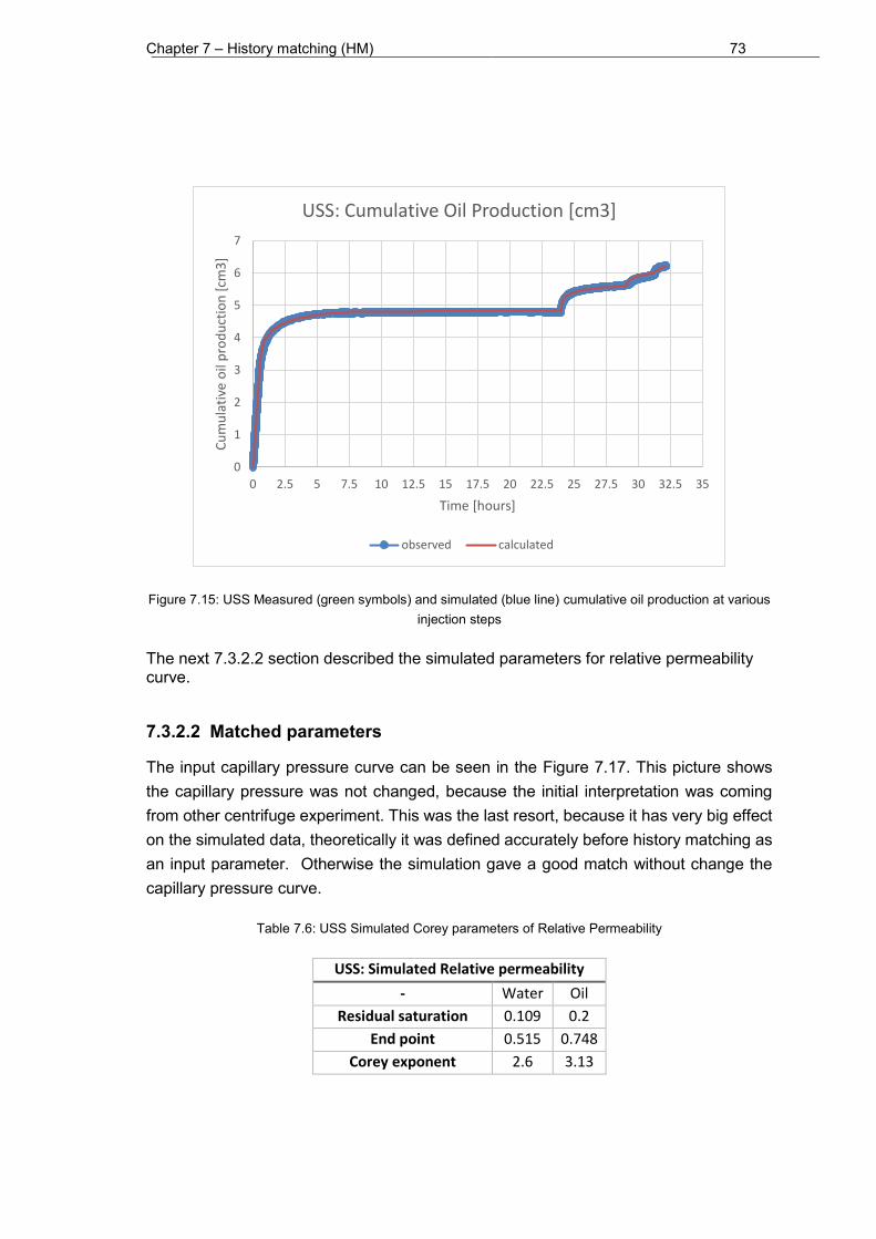
Chapter 7 – History matching (HM) 73
Figure 7.15: USS Measured (green symbols) and simulated (blue line) cumulative oil production at various injection steps
The next 7.3.2.2 section described the simulated parameters for relative permeability curve.
7.3.2.2 Matched parameters
The input capillary pressure curve can be seen in the Figure 7.17. This picture shows the capillary pressure was not changed, because the initial interpretation was coming from other centrifuge experiment. This was the last resort, because it has very big effect on the simulated data, theoretically it was defined accurately before history matching as an input parameter. Otherwise the simulation gave a good match without change the capillary pressure curve.
Table 7.6: USS Simulated Corey parameters of Relative Permeability
USS: Simulated Relative permeability
- Water Oil
Residual saturation 0.109 0.2
End point 0.515 0.748
Corey exponent 2.6 3.13
0
1
2
3
4
5
6
7
0 2.5 5 7.5 10 12.5 15 17.5 20 22.5 25 27.5 30 32.5 35
Cu
mu
lati
ve o
il p
rod
uct
ion
[cm
3]
Time [hours]
USS: Cumulative Oil Production [cm3]
observed calculated
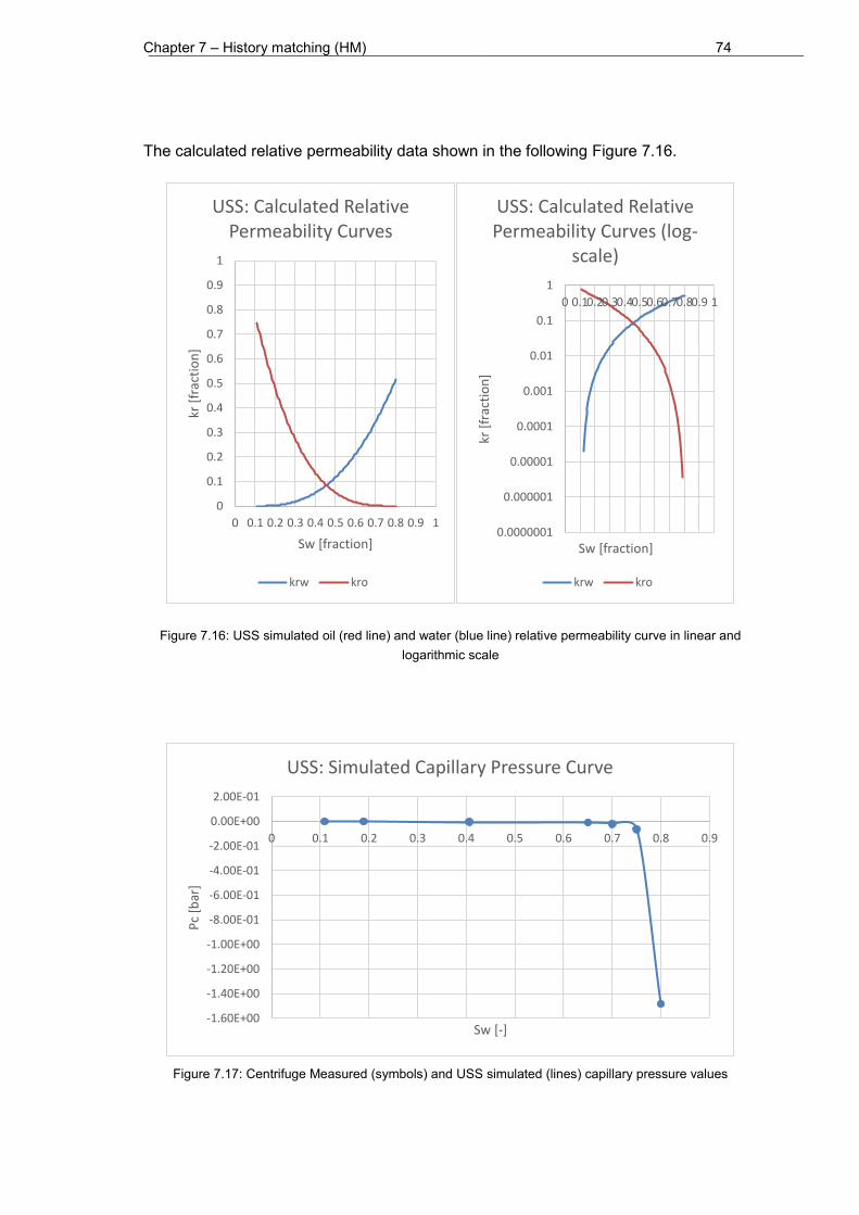
Chapter 7 – History matching (HM) 74
The calculated relative permeability data shown in the following Figure 7.16.
Figure 7.16: USS simulated oil (red line) and water (blue line) relative permeability curve in linear and logarithmic scale
Figure 7.17: Centrifuge Measured (symbols) and USS simulated (lines) capillary pressure values
0
0.1
0.2
0.3
0.4
0.5
0.6
0.7
0.8
0.9
1
0 0.1 0.2 0.3 0.4 0.5 0.6 0.7 0.8 0.9 1
kr [
frac
tio
n]
Sw [fraction]
USS: Calculated Relative Permeability Curves
krw kro
0.0000001
0.000001
0.00001
0.0001
0.001
0.01
0.1
1
0 0.10.20.30.40.50.60.70.80.9 1
kr [
frac
tio
n]
Sw [fraction]
USS: Calculated Relative Permeability Curves (log-
scale)
krw kro
-1.60E+00
-1.40E+00
-1.20E+00
-1.00E+00
-8.00E-01
-6.00E-01
-4.00E-01
-2.00E-01
0.00E+00
2.00E-01
0 0.1 0.2 0.3 0.4 0.5 0.6 0.7 0.8 0.9
Pc
[bar
]
Sw [-]
USS: Simulated Capillary Pressure Curve

Chapter 7 – History matching (HM) 75
7.3.3 Matching Centrifuge data
One real experimental dataset has been used for history matching of the centrifuge measurement. This experiment was a multi-speed centrifuge measurement. The dataset is provided by the advisor of the present thesis. The used fluid and rock listed in the Table 7.7.
Table 7.7: Fluid and rock properties of Centrifuge imbibition measurement
Fluid and rock properties
Data unit
L 4.905 cm
d 3.786 cm
K 25.2 mD
φ 0.292 -
Swc 0.0731 -
Sor 0.065 -
µw 0.00066 Pa.s
µo 0.0014 Pa.s
ρw 1.098 g/cm3
ρo 0.782 g/cm3
The rotation schedule is defined with ten increasing speed steps, shown in Table 7.8. The first seven steps have been performed relatively low speed with small increasing steps, at the end of the centrifuge experiment the last three flood performed with relatively high speed.
Table 7.8: Rotation schedule for Centrifuge measurement
Schedule for Centrifuge
Injection period
Time Gravity in the centre of the
core
[hour] [m/s2]
1 0 843.7
2 48 1499.9
3 99.33 2343.6
4 147.3 3374.8
5 193.2 5999.6
6 240.1 9374.4
7 288.1 18373.8
8 312.1 37497.6
9 330.9 84369.7
10 378.9 181489.6

Chapter 7 – History matching (HM) 76
Centrifuge technique is in essence an unsteady-state technique. The observation data from this experiment are different from SS and USS. During the centrifuge experiment the differential pressure and saturation profile after each speed step along the core has not been measured. The observation data was the average water saturation and the cumulative oil production. The production data is measured only for expelled phase. In this investigated case, the results of imbibition measurement has been matched, it means the expelled phase was oil and the invading phase was water.
In this case the matched data from multi speed centrifuge experiment is just capillary pressure curve, because relative permeability data was available from other experiments. As initial guess capillary pressure was calculated analytically by Hassler-Brunner analysis.
In general, the centrifuge experiment also can be used for interpretation of the relative permeability of expelled phase with only single speed experiment by Hagoort’s analysis. The applied speed during the single-speed should be maximum of the multi-speed experiments. The two experiments are in good agreement if in single-speed experiment the amount of produced fluid is almost the same as in multi-speed experiment. Which indicates the covered saturation range is the same in both cases, the capillary pressure and relative permeability values are interpreted at the same saturation range.
All of the observation data has been matched in good agreement with the developed tool, as can be seen the following 7.3.3.1 part.
7.3.3.1 Observation, Simulated and Matched parameters
The control parameter of the centrifuge model was the rotation speed at each speed step. From the rotation speed the centrifugal acceleration has been calculated and converted into gravity column in the model.
Figure 7.18: Centrifuge speed translated into gravity force (in the center of the core) at each rotation speed step
-200000
-150000
-100000
-50000
0
0 50 100 150 200 250 300 350 400
g [m
/m2]
Time [hour]
Centrifugal Acceleration

Chapter 7 – History matching (HM) 77
On the Figure 7.19 can be seen the simulated water saturation profile of equilibrium state at the end of each speed step.
Figure 7.19: Centrifuge simulated water saturation profile of equilibrium at each rotation speed step
S0 is the initial state, before the rotation starts, which is zero. The average water saturation is constantly increasing with increasing rotation speed along the core. The rotation centre is on the left side of the Figure 7.19, which describes the shape of these curves, the higher water saturation can be seen in the beginning of the core, because the water entre here and continuously expelling the oil phase.
0
0.1
0.2
0.3
0.4
0.5
0.6
0.7
0.8
0.9
1
0 0.5 1 1.5 2 2.5 3 3.5 4 4.5 5
Sw [
frac
tio
n]
Core length [cm]
Centrifuge: Water Saturation Profiles
S0 S1 S2 S3 S4 S5 S6 S7 S8 S9 S10

Chapter 7 – History matching (HM) 78
Figure 7.20: Centrifuge average water saturation of equilibrium state at each rotation speed step
Figure 7.21: Centrifuge measured (blue line) and simulated (red line) cumulative oil production of equilibrium state at each rotation speed step
The simulated average water saturation shown in Figure 7.20 and cumulative oil production data shown in Figure 7.21. These are in good agreement with the measured curves. The only difference which can be observed, the equilibrium parts are matched better, where capillary pressure effects are more dominant. At early stage (curvature) of each speed steps, the relative permeability is playing most significant role. Therefore the difference could be acceptable, explained by deficiencies of provided relative permeability data.
0
0.2
0.4
0.6
0.8
1
0 50 100 150 200 250 300 350 400Sw a
vera
ge [
frac
tio
n]
Time [hour]
Centrifuge: Average Water Saturation
observed calculated
0.00
2.00
4.00
6.00
8.00
10.00
12.00
14.00
0 50 100 150 200 250 300 350 400
Cu
mu
lati
ve o
il p
rod
uct
ion
[cm
3]
Time [hours]
Centrifuge: Cumulative Oil Production [cm3]
observed calculated

Chapter 7 – History matching (HM) 79
Figure 7.22: Centrifuge Simulated Relative Permeability in linear logarithmic scale
As above mentioned the relative permeability data was interpreted based on other experiments, therefore in this case the matched data from multi speed centrifuge experiment was just capillary pressure curve. The relative permeability was just an input parameter.
Only one changes has been applied in relative permeability curve, but this should be the last thing what can be changed, because it is coming from another interpretation.
Table 7.9 : C Simulated Corey parameters of Relative Permeability
C: Simulated Relative permeability
- water oil
Residual saturation 0.0731 0.065
End point 0.8 0.5
Corey exponent 2 4
0
0.1
0.2
0.3
0.4
0.5
0.6
0.7
0.8
0.9
1
0 0.1 0.2 0.3 0.4 0.5 0.6 0.7 0.8 0.9 1
k r[f
ract
ion
]
Sw [fraction]
C: Calculated Relative Permeability Curves
krw kro
0.000001
0.00001
0.0001
0.001
0.01
0.1
1
0 0.10.20.30.40.50.60.70.80.9 1
k r[f
ract
ion
]
Sw [fraction]
C: Calculated Relative Permeability Curves
(in log-scale)
krw kro

Chapter 7 – History matching (HM) 80
Figure 7.23: Measured and Simulated Capillary pressure curves from centrifuge experiment
As initial guess capillary pressure was calculated analytically by Hassler-Brunner analysis and from inflow calculations. The matched simulated capillary pressure is closed to both analytical interpretation, but more or less in-between them. Therefore the numerical history matching calculation is reasonable, to improve the result.
Table 7.10: C Simulated Extended Corey parameters of Capillary Pressure
C: Simulated Capillary Pressure
- water oil
Initial/residual saturation 0.075 0.065
Corey exponent 10 20
Sd 0.5 0.8
Pc(Sd) -0.08 -0.35
-30
-25
-20
-15
-10
-5
0
5
0 0.2 0.4 0.6 0.8 1
Pc
[bar
]
Sw [fraction]
C: Measured and Simulated Capillary Pressure Curves
calculated Pc inflow Hassler-Bruner analysis

Chapter 8 – Summary 81
8 Summary
The present master thesis aims on numerical interpretation of SCAL (Special Core Analysis) data in order to improve the quality of relative permeability and capillary pressure saturation functions.
Relative permeability and capillary pressure are essential to Reservoir Engineering because they determine the efficiency of water-flooding operations on the microscopic and macroscopic scale. These functions are required for predicting the reservoir performance through the whole reservoir life time. Generally, the relative fluid-phase permeability in the formation rock can be measured by performing displacement experiments in core sample by either steady state or unsteady state flooding experiments.
Conventional analytical interpretation of SCAL experiments as performed by many service laboratories may add uncertainty to relative permeability and capillary pressure data and consequently to reservoir simulations. Relative permeability and capillary pressure function are more reliably after proper numerical history matching calculations.
The main problems of the analytical approach are the simplified approximations behind the interpretation models such as the JBN approach [1]. This is the restrictive assumption that neglects action of capillary forces, which is especially a problem close to residual oil saturation.
By numerical history matching of SCAL experimental data typical experimental issues and the deficiencies of analytical interpretation methods can be overcome. In the frame of the thesis, numerical models for different SCAL techniques have been set up and has been used to describe experimental data. To achieve the best interpretation and for better handling, the history matching procedure has been automated.
These numerical models of SS (steady-state), USS (unsteady state) and C (centrifuge) experiments and more specifically history matching of related production, pressure and saturation data are the way to obtain more accurate results because full physics is taken into account.
Finally, the developed models have been verified by comparison of the results obtained in this study to literature data obtained by using different simulation tools and approaches.

Chapter 9 – Conclusion and Outlook 82
9 Conclusion and Outlook
The aim of this work has been to construct numerical core models in order to analyse experimental data and reliably extract relative permeability and capillary pressure saturation functions. With the numerical interpretation, we take full physics into account and overcome the deficiencies of commonly used analytical models. The resulting assisted SCAL history matching tool has been developed in ECLIPSE with the help of Python scripts. Three different models have been constructed related to the type of the SCAL measurements. The developed tool is assisted and automatized control matching tool. Two of the functions, which have the most significant effect on the reservoir simulation results are relative permeability and capillary pressure curves. Critically important is the relative permeability characteristic. These data are usually calculated from laboratory SCAL (Special Core Analysis) measurements using reservoir core samples. The main drawback which arises from analytical approaches is that the calculated values of relative permeability or capillary pressures are coming based on the assumption that only either viscous or capillary forces are acting in the system, but not together.
These analytical interpretations have shown insufficient accuracy especially in comparison to the obtained numerical results. As the present work shows, to decrease the uncertainty of field simulations with respect to relative permeability and capillary pressure, SCAL data need to be interpreted using numerical models as developed here.
Another conclusion of this work, but outside of the scope, is the relative permeability and capillary pressure functions are interdependent characteristics of two-phase flow, which can be most accurately evaluated by performing flooding and centrifuge experiments on the same core sample.
Based on the results, a next step could be make the interpretation models more realistic. The simulations could be performed in 3D and effects like fluid compressibility and other effects could be accounted for. However this means in turn that more complex laboratory data are required. From the history matching point of view, the main interest is in minimizing the solutions non-uniqueness itself by introducing an assisted history matching tool analysing different SCAL experiments simultaneously. The combination of the several type of experiments, and simultaneously match them with the same input parameters can decrease the range of the acceptable solutions, which results in the same objective function. Based on own experience and literature, the history matching algorithm can be improved; the adjoint approach has to be applied to minimize the objective function in the extended version of the core models.

Chapter 9 – Conclusion and Outlook 83
Last but not least the used software, namely ECLIPSE should be changed to Matlab developed reservoir simulator tool – MRST since MRST`s flexibility is higher and the handling is better than in ECLIPSE. The first steps towards a Matlab tool has been made.
Chapter 10 – References 84
10 References
[1] E. F. Johnson, D. P. Bossler and V. O. Naumann, “Calculation of Relative
Permeability from Displacement Experiments,” in Society of Petroleum Engineers,
Tulsa, Okla, 1958.
[2] L. Ganzer and J. Wegner, Reservoir Simulation Methods I (Lecture Notes), Leoben:
HOT Engineering, 2015.
[3] M. Felsenthal, “A Statistical Study of Some Waterflood Parameters (Paper SPE
7666),” JOURNAL OF PETROLEUM TECHNOLOGY, 1979.
[4] H. Ott, Special Core Analysis Lecture Notes, Leoben: Montanuniversität Leoben,
2016.
[5] M. Honarpour, L. Koederitz and A. H. Harvey, Relative Permeability of Petroleum
Reservoirs, Boca Raton, Florida: CRC Press Inc..
[6] J. Bear, Dynamics of fluids in porous media, New York: DOVER PUBLICATION,
INC, 1988.
[7] S. K. Masalmeh, X. Jing, S. Roth, C. Wang and H. Dong, “Towards Predicting Multi-
Phase Flow in Porous Media Using Digital Rock Physics: Workflow to Test the
Predictive Capability of Pore-Scale Modeling. (SPE-177572-MS),” in International
Petroleum Exhibition, Abu Dhabi, 2015.
[8] J. Kleppe, “Norwegian University of Science and Technology, Department of
Petroleum Engineering and Applied Geophysics,” 31 08 2016. [Online]. Available:
http://www.ipt.ntnu.no/~kleppe/TPG4150/BL.pdf.
[9] C. McPhee, J. Reed and I. Zubizarreta, Core Analysis: A Best Practice Guide,
Amsterdam, Oxford, Waltham: Elsevier B.V., 2015.
[10] N. T. Burdine, “Relative permeability calculations from pore-size distribution data.,”
Trans .AIME,, 1952..

Chapter 10 – References 85
[11] Schlumberger. Ltd., ECLIPSE Manual - ECLIPSE Technical Descripton, Texas:
Schlumberger Ltd., 2015.
[12] R. Lenormand, K. Lorentzen, J. G. Maas and D. Ruth, “Comparison of four
numerical simulators for scal experiments (SCA2016-13),” in International
Symposium of the Society of Core Analysts, Snow Mass, Colorado, USA, 2016.
[13] D. S. Oliver, INVERSE THEORY FOR Petroleum Reservoir Characterisation and
History Matching, New York, Melbourne, Madrid, Cape Town, Singapore, São
Paulo: United States of America by Cambridge University Press, 2008.
[14] D. Loeve, “Simultaneous determination of relative permeability and capillary
pressure curves by assisted history matchng several SCAL experiments (2011-
35),” in Society of Core Analysts , Austin, Texas, 2011.
[15] “Open Source Library of Scientific Tools,” [Online]. Available: http://www.scipy.org.
[16] Frode Lomeland, “A new versatile relative permeability correlation (SCA2005-32),”
in International Symposium of the Society of Core Analysts, Toronto, 2005.
[17] H. Ott, C. H. Pentland and S. Oedai, “CO2-brine displacement in heterogeneous
carbonates,” International Journal of Greenhouse Gas Control 33, pp. 135-144,
2015.
[18] J. G. Maas, B. Flemisch and A. Hebig, “Open source simulator DuMuX available
for SCAL interpretation. (SCA2011-08),” in International Symposium of the Society
of Core Analysts, Texas, 2011.
[19] S. K. Masalmeh and X. D. Jing, “The importance of Special Core analysis in
modelling remaining oil saturation in carbonate fields. (SCA2008-03),” in
International Symposium of the Society of Core Analysts, Abu Dhabi, 2008.
[20] S. K. Masalmeh, “Impact of capillary forces on residual saturation and flooding
experiments for mixed to oil-wet carbonate reservoirs. (SCA2012-11),” in
International Symposium of the Society of Core Analysts, Aberdeen, Scotland, UK,
2012.

Chapter 10 – References 86
[21] D. Ruth, “Analysis of centrifuge relative permeability data (SCA-9711),” in
International Symposium of the Society of Core Analysts, Winnipeg, Manitoba,
Canada, 1997.
[22] L. Ganzer and J. Wegner, Reservoir Simulation Methods II. (Lecture Notes),
Leoben: Hot Engineering, 2015.

Appendices 87
Appendices Appendix A - SS_SCAL.data RUNSPEC TITLE SS_SCAL START 1 'JAN' 2016 / LAB OIL WATER -- this keyword requests that information required for the run-time monitoring option should be written to the Summary Specification file MONITOR -- requests that a Restart Index file should be written at the end of the run RSSPEC -- The message file feature is provided primarily for use by post-processors MSGFILE 0 / -- this indicates that output files will be formatted -- this includes SMSPEC, SUMMARY, GRID, INIT and RESTART files FMTOUT -- this indicates that output files will be unified -- this includes SMSPEC, SUMMARY, GRID, INIT and RESTART files UNIFOUT -- this indicates that the saturation table end-point scaling option is to be used --ENDSCALE --'NODIR' 'REVERS' 1 20 / WELLDIMS -- max. number of wells number of layers( grid blocks ) connected to the well max number of groups max. number of wells in one group default values 4 52 5 4 / -- max number of related fluid model quantities TABDIMS -- num of saturation tables num of pvt tables num of saturation nodes num of pressure points in PVT table num of FIP regions 2 1 50 1* 2 / DIMENS -- specifies the dimensions of the grid [ nx ny nz ] 52 1 1 / GRID NOECHO INCLUDE './include/SS_SCAL_GOPP.INC' /

Appendices 88
INCLUDE './include/SS_SCAL_GGO.INC' / INCLUDE './include/SS_SCAL_GPRO.INC' / EDIT PROPS NOECHO INCLUDE './include/SS_SCAL_PVT.INC' / INCLUDE './include/SS_SCAL_SCAL.INC' / INCLUDE './include/SS_SCAL_SWOF.INC' / REGIONS NOECHO INCLUDE './include/SS_SCAL_REG.INC' / SOLUTION NOECHO RPTRST BASIC=2 / INCLUDE './include/SS_SCAL_INIT.INC' / RPTRST BASIC=2 PRESSURE SWAT SOIL / SUMMARY NOECHO INCLUDE -- Generated : Petrel './include/SS_SCAL_SUM.INC' / SCHEDULE NOECHO RPTSCHED RESTART 'NEWTON=2' / INCLUDE -- Generated : Petrel './include/SS_SCAL_SCH.INC' / INCLUDE './include/SS_SCAL_WELLSCH.INC' / SAVE END
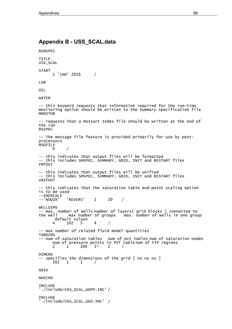
Appendices 89
Appendix B - USS_SCAL.data RUNSPEC TITLE USS_SCAL START 1 'JAN' 2016 / LAB OIL WATER -- this keyword requests that information required for the run-time monitoring option should be written to the Summary Specification file MONITOR -- requests that a Restart Index file should be written at the end of the run RSSPEC -- The message file feature is provided primarily for use by post-processors MSGFILE 0 / -- this indicates that output files will be formatted -- this includes SMSPEC, SUMMARY, GRID, INIT and RESTART files FMTOUT -- this indicates that output files will be unified -- this includes SMSPEC, SUMMARY, GRID, INIT and RESTART files UNIFOUT -- this indicates that the saturation table end-point scaling option is to be used --ENDSCALE --'NODIR' 'REVERS' 1 20 / WELLDIMS -- max. number of wells number of layers( grid blocks ) connected to the well max number of groups max. number of wells in one group default values 4 102 5 4 / -- max number of related fluid model quantities TABDIMS -- num of saturation tables num of pvt tables num of saturation nodes num of pressure points in PVT table num of FIP regions 2 1 100 1* 2 / DIMENS -- specifies the dimensions of the grid [ nx ny nz ] 102 1 1 / GRID NOECHO INCLUDE './include/USS_SCAL_GOPP.INC' / INCLUDE './include/USS_SCAL_GGO.INC' /

Appendices 90
INCLUDE './include/USS_SCAL_GPRO.INC' / EDIT PROPS NOECHO INCLUDE './include/USS_SCAL_PVT.INC' / INCLUDE './include/USS_SCAL_SCAL.INC' / INCLUDE './include/USS_SCAL_SWOF.INC' / REGIONS NOECHO INCLUDE './include/USS_SCAL_REG.INC' / SOLUTION NOECHO RPTRST BASIC=2 / INCLUDE './include/USS_SCAL_INIT.INC' / SUMMARY NOECHO INCLUDE -- Generated : Petrel './include/USS_SCAL_SUM.INC' / SCHEDULE NOECHO RPTSCHED RESTART 'NEWTON=2' / INCLUDE -- Generated : Petrel './include/USS_SCAL_SCH.INC' / INCLUDE './include/USS_SCAL_WELLSCH.INC' / SAVE END
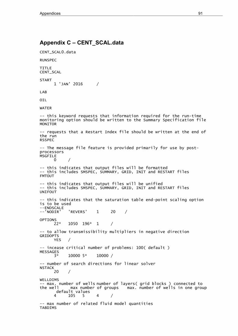
Appendices 91
Appendix C – CENT_SCAL.data CENT_SCAL0.data RUNSPEC TITLE CENT_SCAL START 1 'JAN' 2016 / LAB OIL WATER -- this keyword requests that information required for the run-time monitoring option should be written to the Summary Specification file MONITOR -- requests that a Restart Index file should be written at the end of the run RSSPEC -- The message file feature is provided primarily for use by post-processors MSGFILE 0 / -- this indicates that output files will be formatted -- this includes SMSPEC, SUMMARY, GRID, INIT and RESTART files FMTOUT -- this indicates that output files will be unified -- this includes SMSPEC, SUMMARY, GRID, INIT and RESTART files UNIFOUT -- this indicates that the saturation table end-point scaling option is to be used --ENDSCALE --'NODIR' 'REVERS' 1 20 / OPTIONS 22* 1050 196* 1 / -- to allow transmissibility multipliers in negative direction GRIDOPTS YES / -- incease critical number of problems: 100( default ) MESSAGES 3* 10000 5* 10000 / -- number of search directions for linear solver NSTACK 20 / WELLDIMS -- max. number of wells number of layers( grid blocks ) connected to the well max number of groups max. number of wells in one group default values 4 105 5 4 / -- max number of related fluid model quantities TABDIMS

Appendices 92
-- num of saturation tables num of pvt tables num of saturation nodes num of pressure points in PVT table num of FIP regions 2 105 100 1* 2 / DIMENS -- specifies the dimensions of the grid [ nx ny nz ] 3 1 105 / GRID NOECHO INCLUDE './include/CENT_SCAL_GOPP.INC' / INCLUDE './include/CENT_SCAL_GGO.INC' / INCLUDE './include/CENT_SCAL_GPRO.INC' / PROPS NOECHO GRAVCONS -- gravity acceleration [cm2atm/gm], default value: 0.000968 0.068336 / INCLUDE './include/CENT_SCAL_PVT.INC' / INCLUDE './include/CENT_SCAL_SCAL.INC' / INCLUDE './include/CENT_SCAL_SWOF.INC' / REGIONS NOECHO INCLUDE './include/CENT_SCAL_REG.INC' / SOLUTION NOECHO RPTRST BASIC=2 / INCLUDE './include/CENT_SCAL_INIT0.INC' / SUMMARY NOECHO INCLUDE './include/CENT_SCAL_SUM.INC' / SCHEDULE NOECHO RPTSCHED RESTART 'NEWTON=2' /

Appendices 93
INCLUDE './include/CENT_SCAL_SCH.INC' / INCLUDE './include/CENT_SCAL_WELLSCH0.INC' / SAVE END CENT_SCAL1.data RUNSPEC TITLE CENT_SCAL START 1 'JAN' 2016 / LAB OIL WATER -- this keyword requests that information required for the run-time monitoring option should be written to the Summary Specification file MONITOR -- requests that a Restart Index file should be written at the end of the run RSSPEC -- The message file feature is provided primarily for use by post-processors MSGFILE 0 / -- this indicates that output files will be formatted -- this includes SMSPEC, SUMMARY, GRID, INIT and RESTART files FMTOUT -- this indicates that output files will be unified -- this includes SMSPEC, SUMMARY, GRID, INIT and RESTART files UNIFOUT -- This indicates that input files which may be either formatted or unformatted, such as restart files, are to be formatted FMTIN -- This indicates that input files (for example Restart files), which may be either multiple or unified, are unified UNIFIN --SAVE -- save data to unified formatted file -- FORMATTED / -- this indicates that the saturation table end-point scaling option is to be used --ENDSCALE --'NODIR' 'REVERS' 1 20 / OPTIONS

Appendices 94
22* 1050 196* 1 / -- to allow transmissibility multipliers in negative direction GRIDOPTS YES / -- incease critical number of problems: 100( default ) MESSAGES 3* 10000 5* 10000 / -- number of search directions for linear solver NSTACK 20 / WELLDIMS -- max. number of wells number of layers( grid blocks ) connected to the well max number of groups max. number of wells in one group default values 4 105 5 4 / -- max number of related fluid model quantities TABDIMS -- num of saturation tables num of pvt tables num of saturation nodes num of pressure points in PVT table num of FIP regions 2 105 100 1* 2 / DIMENS -- specifies the dimensions of the grid [ nx ny nz ] 3 1 105 / GRID NOECHO INCLUDE './include/CENT_SCAL_GOPP.INC' / INCLUDE './include/CENT_SCAL_GGO.INC' / INCLUDE './include/CENT_SCAL_GPRO.INC' / PROPS NOECHO GRAVCONS -- gravity acceleration [cm2atm/gm], default value: 0.000968 0.121486 / INCLUDE './include/CENT_SCAL_PVT.INC' / INCLUDE './include/CENT_SCAL_SCAL.INC' / INCLUDE './include/CENT_SCAL_SWOF.INC' / REGIONS NOECHO INCLUDE './include/CENT_SCAL_REG.INC' / SOLUTION
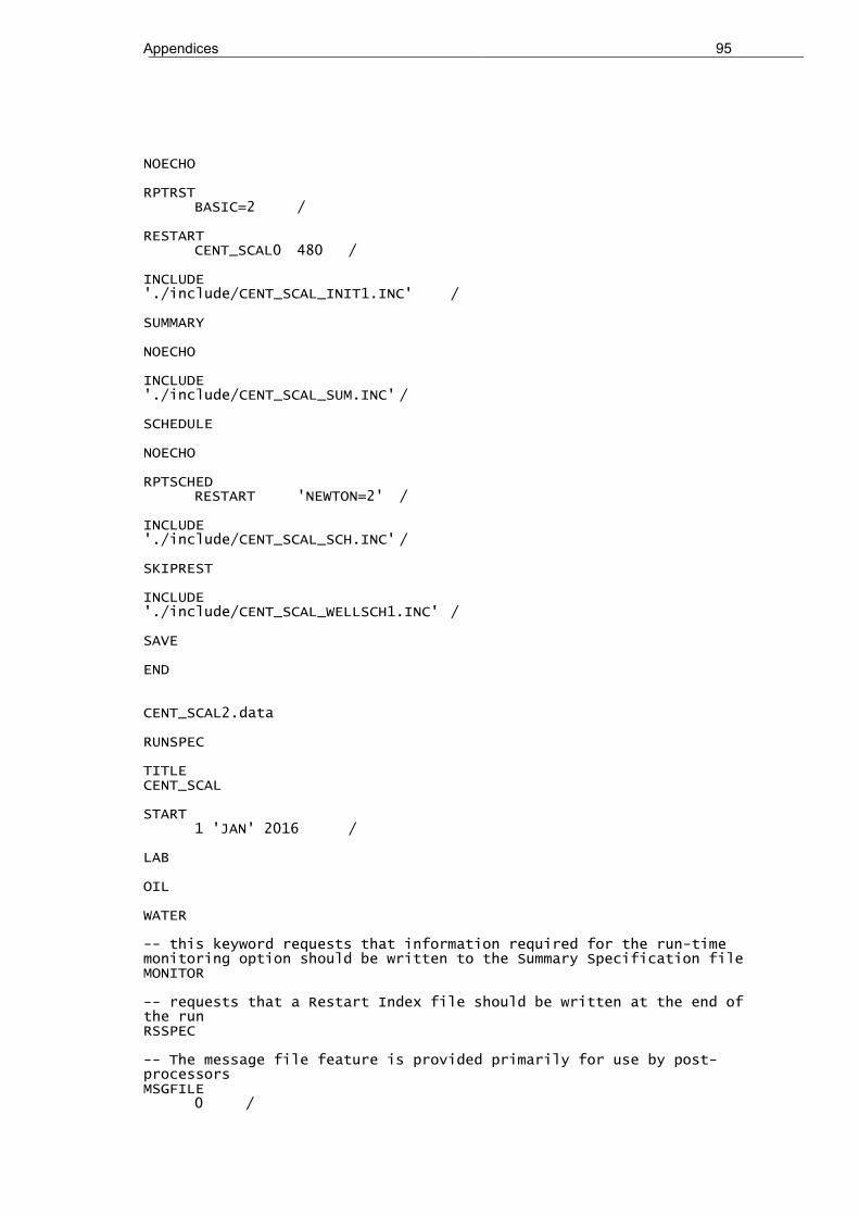
Appendices 95
NOECHO RPTRST BASIC=2 / RESTART CENT_SCAL0 480 / INCLUDE './include/CENT_SCAL_INIT1.INC' / SUMMARY NOECHO INCLUDE './include/CENT_SCAL_SUM.INC' / SCHEDULE NOECHO RPTSCHED RESTART 'NEWTON=2' / INCLUDE './include/CENT_SCAL_SCH.INC' / SKIPREST INCLUDE './include/CENT_SCAL_WELLSCH1.INC' / SAVE END CENT_SCAL2.data RUNSPEC TITLE CENT_SCAL START 1 'JAN' 2016 / LAB OIL WATER -- this keyword requests that information required for the run-time monitoring option should be written to the Summary Specification file MONITOR -- requests that a Restart Index file should be written at the end of the run RSSPEC -- The message file feature is provided primarily for use by post-processors MSGFILE 0 /
Appendices 96
-- this indicates that output files will be formatted -- this includes SMSPEC, SUMMARY, GRID, INIT and RESTART files FMTOUT -- this indicates that output files will be unified -- this includes SMSPEC, SUMMARY, GRID, INIT and RESTART files UNIFOUT -- This indicates that input files which may be either formatted or unformatted, such as restart files, are to be formatted FMTIN -- This indicates that input files (for example Restart files), which may be either multiple or unified, are unified UNIFIN --SAVE -- save data to unified formatted file -- FORMATTED / -- this indicates that the saturation table end-point scaling option is to be used --ENDSCALE --'NODIR' 'REVERS' 1 20 / OPTIONS 22* 1050 196* 1 / -- to allow transmissibility multipliers in negative direction GRIDOPTS YES / -- incease critical number of problems: 100( default ) MESSAGES 3* 10000 5* 10000 / -- number of search directions for linear solver NSTACK 20 / WELLDIMS -- max. number of wells number of layers( grid blocks ) connected to the well max number of groups max. number of wells in one group default values 4 105 5 4 / -- max number of related fluid model quantities TABDIMS -- num of saturation tables num of pvt tables num of saturation nodes num of pressure points in PVT table num of FIP regions 2 105 100 1* 2 / DIMENS -- specifies the dimensions of the grid [ nx ny nz ] 3 1 105 / GRID NOECHO INCLUDE './include/CENT_SCAL_GOPP.INC' / INCLUDE './include/CENT_SCAL_GGO.INC' / INCLUDE './include/CENT_SCAL_GPRO.INC' /
Appendices 97
PROPS NOECHO GRAVCONS -- gravity acceleration [cm2atm/gm], default value: 0.000968 0.189822 / INCLUDE './include/CENT_SCAL_PVT.INC' / INCLUDE './include/CENT_SCAL_SCAL.INC' / INCLUDE './include/CENT_SCAL_SWOF.INC' / REGIONS NOECHO INCLUDE './include/CENT_SCAL_REG.INC' / SOLUTION NOECHO RPTRST BASIC=2 / RESTART CENT_SCAL1 994 / INCLUDE './include/CENT_SCAL_INIT2.INC' / SUMMARY NOECHO INCLUDE './include/CENT_SCAL_SUM.INC' / SCHEDULE NOECHO RPTSCHED RESTART 'NEWTON=2' / INCLUDE './include/CENT_SCAL_SCH.INC' / SKIPREST INCLUDE './include/CENT_SCAL_WELLSCH2.INC' / SAVE END

Appendices 98
CENT_SCAL3.data RUNSPEC TITLE CENT_SCAL START 1 'JAN' 2016 / LAB OIL WATER -- this keyword requests that information required for the run-time monitoring option should be written to the Summary Specification file MONITOR -- requests that a Restart Index file should be written at the end of the run RSSPEC -- The message file feature is provided primarily for use by post-processors MSGFILE 0 / -- this indicates that output files will be formatted -- this includes SMSPEC, SUMMARY, GRID, INIT and RESTART files FMTOUT -- this indicates that output files will be unified -- this includes SMSPEC, SUMMARY, GRID, INIT and RESTART files UNIFOUT -- This indicates that input files which may be either formatted or unformatted, such as restart files, are to be formatted FMTIN -- This indicates that input files (for example Restart files), which may be either multiple or unified, are unified UNIFIN --SAVE -- save data to unified formatted file -- FORMATTED / -- this indicates that the saturation table end-point scaling option is to be used --ENDSCALE --'NODIR' 'REVERS' 1 20 / OPTIONS 22* 1050 196* 1 / -- to allow transmissibility multipliers in negative direction GRIDOPTS YES / -- incease critical number of problems: 100( default ) MESSAGES 3* 10000 5* 10000 / -- number of search directions for linear solver NSTACK 20 /

Appendices 99
WELLDIMS -- max. number of wells number of layers( grid blocks ) connected to the well max number of groups max. number of wells in one group default values 4 105 5 4 / -- max number of related fluid model quantities TABDIMS -- num of saturation tables num of pvt tables num of saturation nodes num of pressure points in PVT table num of FIP regions 2 105 100 1* 2 / DIMENS -- specifies the dimensions of the grid [ nx ny nz ] 3 1 105 / GRID NOECHO INCLUDE './include/CENT_SCAL_GOPP.INC' / INCLUDE './include/CENT_SCAL_GGO.INC' / INCLUDE './include/CENT_SCAL_GPRO.INC' / PROPS NOECHO GRAVCONS -- gravity acceleration [cm2atm/gm], default value: 0.000968 0.273345 / INCLUDE './include/CENT_SCAL_PVT.INC' / INCLUDE './include/CENT_SCAL_SCAL.INC' / INCLUDE './include/CENT_SCAL_SWOF.INC' / REGIONS NOECHO INCLUDE './include/CENT_SCAL_REG.INC' / SOLUTION NOECHO RPTRST BASIC=2 / RESTART CENT_SCAL2 1474 / INCLUDE './include/CENT_SCAL_INIT3.INC' / SUMMARY

Appendices 100
NOECHO INCLUDE './include/CENT_SCAL_SUM.INC' / SCHEDULE NOECHO RPTSCHED RESTART 'NEWTON=2' / INCLUDE './include/CENT_SCAL_SCH.INC' / SKIPREST INCLUDE './include/CENT_SCAL_WELLSCH3.INC' / SAVE END CENT_SCAL4.data RUNSPEC TITLE CENT_SCAL START 1 'JAN' 2016 / LAB OIL WATER -- this keyword requests that information required for the run-time monitoring option should be written to the Summary Specification file MONITOR -- requests that a Restart Index file should be written at the end of the run RSSPEC -- The message file feature is provided primarily for use by post-processors MSGFILE 0 / -- this indicates that output files will be formatted -- this includes SMSPEC, SUMMARY, GRID, INIT and RESTART files FMTOUT -- this indicates that output files will be unified -- this includes SMSPEC, SUMMARY, GRID, INIT and RESTART files UNIFOUT -- This indicates that input files which may be either formatted or unformatted, such as restart files, are to be formatted FMTIN

Appendices 101
-- This indicates that input files (for example Restart files), which may be either multiple or unified, are unified UNIFIN --SAVE -- save data to unified formatted file -- FORMATTED / -- this indicates that the saturation table end-point scaling option is to be used --ENDSCALE --'NODIR' 'REVERS' 1 20 / OPTIONS 22* 1050 196* 1 / -- to allow transmissibility multipliers in negative direction GRIDOPTS YES / -- incease critical number of problems: 100( default ) MESSAGES 3* 10000 5* 10000 / -- number of search directions for linear solver NSTACK 20 / WELLDIMS -- max. number of wells number of layers( grid blocks ) connected to the well max number of groups max. number of wells in one group default values 4 105 5 4 / -- max number of related fluid model quantities TABDIMS -- num of saturation tables num of pvt tables num of saturation nodes num of pressure points in PVT table num of FIP regions 2 105 100 1* 2 / DIMENS -- specifies the dimensions of the grid [ nx ny nz ] 3 1 105 / GRID NOECHO INCLUDE './include/CENT_SCAL_GOPP.INC' / INCLUDE './include/CENT_SCAL_GGO.INC' / INCLUDE './include/CENT_SCAL_GPRO.INC' / PROPS NOECHO GRAVCONS -- gravity acceleration [cm2atm/gm], default value: 0.000968 0.485943 / INCLUDE './include/CENT_SCAL_PVT.INC' /
Appendices 102
INCLUDE './include/CENT_SCAL_SCAL.INC' / INCLUDE './include/CENT_SCAL_SWOF.INC' / REGIONS NOECHO INCLUDE './include/CENT_SCAL_REG.INC' / SOLUTION NOECHO RPTRST BASIC=2 / RESTART CENT_SCAL3 1933 / INCLUDE './include/CENT_SCAL_INIT4.INC' / SUMMARY NOECHO INCLUDE './include/CENT_SCAL_SUM.INC' / SCHEDULE NOECHO RPTSCHED RESTART 'NEWTON=2' / INCLUDE './include/CENT_SCAL_SCH.INC' / SKIPREST INCLUDE './include/CENT_SCAL_WELLSCH4.INC' / SAVE END CENT_SCAL5.data RUNSPEC TITLE CENT_SCAL START 1 'JAN' 2016 / LAB OIL WATER

Appendices 103
-- this keyword requests that information required for the run-time monitoring option should be written to the Summary Specification file MONITOR -- requests that a Restart Index file should be written at the end of the run RSSPEC -- The message file feature is provided primarily for use by post-processors MSGFILE 0 / -- this indicates that output files will be formatted -- this includes SMSPEC, SUMMARY, GRID, INIT and RESTART files FMTOUT -- this indicates that output files will be unified -- this includes SMSPEC, SUMMARY, GRID, INIT and RESTART files UNIFOUT -- This indicates that input files which may be either formatted or unformatted, such as restart files, are to be formatted FMTIN -- This indicates that input files (for example Restart files), which may be either multiple or unified, are unified UNIFIN --SAVE -- save data to unified formatted file -- FORMATTED / -- this indicates that the saturation table end-point scaling option is to be used --ENDSCALE --'NODIR' 'REVERS' 1 20 / OPTIONS 22* 1050 196* 1 / -- to allow transmissibility multipliers in negative direction GRIDOPTS YES / -- incease critical number of problems: 100( default ) MESSAGES 3* 10000 5* 10000 / -- number of search directions for linear solver NSTACK 20 / WELLDIMS -- max. number of wells number of layers( grid blocks ) connected to the well max number of groups max. number of wells in one group default values 4 105 5 4 / -- max number of related fluid model quantities TABDIMS -- num of saturation tables num of pvt tables num of saturation nodes num of pressure points in PVT table num of FIP regions 2 105 100 1* 2 / DIMENS -- specifies the dimensions of the grid [ nx ny nz ]
Appendices 104
3 1 105 / GRID NOECHO INCLUDE './include/CENT_SCAL_GOPP.INC' / INCLUDE './include/CENT_SCAL_GGO.INC' / INCLUDE './include/CENT_SCAL_GPRO.INC' / PROPS NOECHO GRAVCONS -- gravity acceleration [cm2atm/gm], default value: 0.000968 0.759288 / INCLUDE './include/CENT_SCAL_PVT.INC' / INCLUDE './include/CENT_SCAL_SCAL.INC' / INCLUDE './include/CENT_SCAL_SWOF.INC' / REGIONS NOECHO INCLUDE './include/CENT_SCAL_REG.INC' / SOLUTION NOECHO RPTRST BASIC=2 / RESTART CENT_SCAL4 2402 / INCLUDE './include/CENT_SCAL_INIT5.INC' / SUMMARY NOECHO INCLUDE './include/CENT_SCAL_SUM.INC' / SCHEDULE NOECHO RPTSCHED RESTART 'NEWTON=2' / INCLUDE './include/CENT_SCAL_SCH.INC' /

Appendices 105
SKIPREST INCLUDE './include/CENT_SCAL_WELLSCH5.INC' / SAVE END CENT_SCAL6.data RUNSPEC TITLE CENT_SCAL START 1 'JAN' 2016 / LAB OIL WATER -- this keyword requests that information required for the run-time monitoring option should be written to the Summary Specification file MONITOR -- requests that a Restart Index file should be written at the end of the run RSSPEC -- The message file feature is provided primarily for use by post-processors MSGFILE 0 / -- this indicates that output files will be formatted -- this includes SMSPEC, SUMMARY, GRID, INIT and RESTART files FMTOUT -- this indicates that output files will be unified -- this includes SMSPEC, SUMMARY, GRID, INIT and RESTART files UNIFOUT -- This indicates that input files which may be either formatted or unformatted, such as restart files, are to be formatted FMTIN -- This indicates that input files (for example Restart files), which may be either multiple or unified, are unified UNIFIN --SAVE -- save data to unified formatted file -- FORMATTED / -- this indicates that the saturation table end-point scaling option is to be used --ENDSCALE --'NODIR' 'REVERS' 1 20 / OPTIONS 22* 1050 196* 1 /

Appendices 106
-- to allow transmissibility multipliers in negative direction GRIDOPTS YES / -- incease critical number of problems: 100( default ) MESSAGES 3* 10000 5* 10000 / -- number of search directions for linear solver NSTACK 20 / WELLDIMS -- max. number of wells number of layers( grid blocks ) connected to the well max number of groups max. number of wells in one group default values 4 105 5 4 / -- max number of related fluid model quantities TABDIMS -- num of saturation tables num of pvt tables num of saturation nodes num of pressure points in PVT table num of FIP regions 2 105 100 1* 2 / DIMENS -- specifies the dimensions of the grid [ nx ny nz ] 3 1 105 / GRID NOECHO INCLUDE './include/CENT_SCAL_GOPP.INC' / INCLUDE './include/CENT_SCAL_GGO.INC' / INCLUDE './include/CENT_SCAL_GPRO.INC' / PROPS NOECHO GRAVCONS -- gravity acceleration [cm2atm/gm], default value: 0.000968 1.488202 / INCLUDE './include/CENT_SCAL_PVT.INC' / INCLUDE './include/CENT_SCAL_SCAL.INC' / INCLUDE './include/CENT_SCAL_SWOF.INC' / REGIONS NOECHO INCLUDE './include/CENT_SCAL_REG.INC' / SOLUTION NOECHO
Appendices 107
RPTRST BASIC=2 / RESTART CENT_SCAL5 2882 / INCLUDE './include/CENT_SCAL_INIT6.INC' / SUMMARY NOECHO INCLUDE './include/CENT_SCAL_SUM.INC' / SCHEDULE NOECHO RPTSCHED RESTART 'NEWTON=2' / INCLUDE './include/CENT_SCAL_SCH.INC' / SKIPREST INCLUDE './include/CENT_SCAL_WELLSCH6.INC' / SAVE END CENT_SCAL7.data RUNSPEC TITLE CENT_SCAL START 1 'JAN' 2016 / LAB OIL WATER -- this keyword requests that information required for the run-time monitoring option should be written to the Summary Specification file MONITOR -- requests that a Restart Index file should be written at the end of the run RSSPEC -- The message file feature is provided primarily for use by post-processors MSGFILE 0 / -- this indicates that output files will be formatted -- this includes SMSPEC, SUMMARY, GRID, INIT and RESTART files

Appendices 108
FMTOUT -- this indicates that output files will be unified -- this includes SMSPEC, SUMMARY, GRID, INIT and RESTART files UNIFOUT -- This indicates that input files which may be either formatted or unformatted, such as restart files, are to be formatted FMTIN -- This indicates that input files (for example Restart files), which may be either multiple or unified, are unified UNIFIN --SAVE -- save data to unified formatted file -- FORMATTED / -- this indicates that the saturation table end-point scaling option is to be used --ENDSCALE --'NODIR' 'REVERS' 1 20 / OPTIONS 22* 1050 196* 1 / -- to allow transmissibility multipliers in negative direction GRIDOPTS YES / -- incease critical number of problems: 100( default ) MESSAGES 3* 10000 5* 10000 / -- number of search directions for linear solver NSTACK 20 / WELLDIMS -- max. number of wells number of layers( grid blocks ) connected to the well max number of groups max. number of wells in one group default values 4 105 5 4 / -- max number of related fluid model quantities TABDIMS -- num of saturation tables num of pvt tables num of saturation nodes num of pressure points in PVT table num of FIP regions 2 105 100 1* 2 / DIMENS -- specifies the dimensions of the grid [ nx ny nz ] 3 1 105 / GRID NOECHO INCLUDE './include/CENT_SCAL_GOPP.INC' / INCLUDE './include/CENT_SCAL_GGO.INC' / INCLUDE './include/CENT_SCAL_GPRO.INC' / PROPS

Appendices 109
NOECHO GRAVCONS -- gravity acceleration [cm2atm/gm], default value: 0.000968 3.037152 / INCLUDE './include/CENT_SCAL_PVT.INC' / INCLUDE './include/CENT_SCAL_SCAL.INC' / INCLUDE './include/CENT_SCAL_SWOF.INC' / REGIONS NOECHO INCLUDE './include/CENT_SCAL_REG.INC' / SOLUTION NOECHO RPTRST BASIC=2 / RESTART CENT_SCAL6 3122 / INCLUDE './include/CENT_SCAL_INIT7.INC' / SUMMARY NOECHO INCLUDE './include/CENT_SCAL_SUM.INC' / SCHEDULE NOECHO RPTSCHED RESTART 'NEWTON=2' / INCLUDE './include/CENT_SCAL_SCH.INC' / SKIPREST INCLUDE './include/CENT_SCAL_WELLSCH7.INC' / SAVE END

Appendices 110
CENT_SCAL8.data RUNSPEC TITLE CENT_SCAL START 1 'JAN' 2016 / LAB OIL WATER -- this keyword requests that information required for the run-time monitoring option should be written to the Summary Specification file MONITOR -- requests that a Restart Index file should be written at the end of the run RSSPEC -- The message file feature is provided primarily for use by post-processors MSGFILE 0 / -- this indicates that output files will be formatted -- this includes SMSPEC, SUMMARY, GRID, INIT and RESTART files FMTOUT -- this indicates that output files will be unified -- this includes SMSPEC, SUMMARY, GRID, INIT and RESTART files UNIFOUT -- This indicates that input files which may be either formatted or unformatted, such as restart files, are to be formatted FMTIN -- This indicates that input files (for example Restart files), which may be either multiple or unified, are unified UNIFIN --SAVE -- save data to unified formatted file -- FORMATTED / -- this indicates that the saturation table end-point scaling option is to be used --ENDSCALE --'NODIR' 'REVERS' 1 20 / OPTIONS 22* 1050 196* 1 / -- to allow transmissibility multipliers in negative direction GRIDOPTS YES / -- incease critical number of problems: 100( default ) MESSAGES 3* 10000 5* 10000 / -- number of search directions for linear solver NSTACK 20 /
Appendices 111
WELLDIMS -- max. number of wells number of layers( grid blocks ) connected to the well max number of groups max. number of wells in one group default values 4 105 5 4 / -- max number of related fluid model quantities TABDIMS -- num of saturation tables num of pvt tables num of saturation nodes num of pressure points in PVT table num of FIP regions 2 105 100 1* 2 / DIMENS -- specifies the dimensions of the grid [ nx ny nz ] 3 1 105 / GRID NOECHO INCLUDE './include/CENT_SCAL_GOPP.INC' / INCLUDE './include/CENT_SCAL_GGO.INC' / INCLUDE './include/CENT_SCAL_GPRO.INC' / PROPS NOECHO GRAVCONS -- gravity acceleration [cm2atm/gm], default value: 0.000968 6.833599 / INCLUDE './include/CENT_SCAL_PVT.INC' / INCLUDE './include/CENT_SCAL_SCAL.INC' / INCLUDE './include/CENT_SCAL_SWOF.INC' / REGIONS NOECHO INCLUDE './include/CENT_SCAL_REG.INC' / SOLUTION NOECHO RPTRST BASIC=2 / RESTART CENT_SCAL7 3310 / INCLUDE './include/CENT_SCAL_INIT8.INC' / SUMMARY

Appendices 112
NOECHO INCLUDE './include/CENT_SCAL_SUM.INC' / SCHEDULE NOECHO RPTSCHED RESTART 'NEWTON=2' / INCLUDE './include/CENT_SCAL_SCH.INC' / SKIPREST INCLUDE './include/CENT_SCAL_WELLSCH8.INC' / SAVE END CENT_SCAL9.data RUNSPEC TITLE CENT_SCAL START 1 'JAN' 2016 / LAB OIL WATER -- this keyword requests that information required for the run-time monitoring option should be written to the Summary Specification file MONITOR -- requests that a Restart Index file should be written at the end of the run RSSPEC -- The message file feature is provided primarily for use by post-processors MSGFILE 0 / -- this indicates that output files will be formatted -- this includes SMSPEC, SUMMARY, GRID, INIT and RESTART files FMTOUT -- this indicates that output files will be unified -- this includes SMSPEC, SUMMARY, GRID, INIT and RESTART files UNIFOUT -- This indicates that input files which may be either formatted or unformatted, such as restart files, are to be formatted FMTIN
Appendices 113
-- This indicates that input files (for example Restart files), which may be either multiple or unified, are unified UNIFIN --SAVE -- save data to unified formatted file -- FORMATTED / -- this indicates that the saturation table end-point scaling option is to be used --ENDSCALE --'NODIR' 'REVERS' 1 20 / OPTIONS 22* 1050 196* 1 / -- to allow transmissibility multipliers in negative direction GRIDOPTS YES / -- incease critical number of problems: 100( default ) MESSAGES 3* 10000 5* 10000 / -- number of search directions for linear solver NSTACK 20 / WELLDIMS -- max. number of wells number of layers( grid blocks ) connected to the well max number of groups max. number of wells in one group default values 4 105 5 4 / -- max number of related fluid model quantities TABDIMS -- num of saturation tables num of pvt tables num of saturation nodes num of pressure points in PVT table num of FIP regions 2 105 100 1* 2 / DIMENS -- specifies the dimensions of the grid [ nx ny nz ] 3 1 105 / GRID NOECHO INCLUDE './include/CENT_SCAL_GOPP.INC' / INCLUDE './include/CENT_SCAL_GGO.INC' / INCLUDE './include/CENT_SCAL_GPRO.INC' / PROPS NOECHO GRAVCONS -- gravity acceleration [cm2atm/gm], default value: 0.000968 14.699832 / INCLUDE './include/CENT_SCAL_PVT.INC' /

Appendices 114
INCLUDE './include/CENT_SCAL_SCAL.INC' / INCLUDE './include/CENT_SCAL_SWOF.INC' / REGIONS NOECHO INCLUDE './include/CENT_SCAL_REG.INC' / SOLUTION NOECHO RPTRST BASIC=2 / RESTART CENT_SCAL8 3790 / INCLUDE './include/CENT_SCAL_INIT9.INC' / SUMMARY NOECHO INCLUDE './include/CENT_SCAL_SUM.INC' / SCHEDULE NOECHO RPTSCHED RESTART 'NEWTON=2' / INCLUDE './include/CENT_SCAL_SCH.INC' / SKIPREST INCLUDE './include/CENT_SCAL_WELLSCH9.INC' / SAVE END