Historical Presidential Betting Markets

Paul W. Rhode and Koleman S. Strumpf

Paul W. Rhode is Professor of Economics and Koleman S. Strumpf is Associate

Professor of Economics, both at the University of North Carolina, Chapel Hill, North

Carolina. Rhode is also a Research Associate, National Bureau of Economic Research,

Cambridge, Massachusetts. Their e-mail addresses are <prhode@email.unc.edu> and

<cigar@unc.edu>, respectively.

1

Wagering on political outcomes has a long history in the United States. As Henry

David Thoreau noted in 1848, “All voting is a sort of gaming,… and betting naturally

accompanies it” (Thoreau, 1967, p. 36). This paper analyzes the large and often well-

organized markets for betting on presidential elections that operated between 1868 and

1940. Over $165 million (in 2002 dollars) was wagered in one election, and betting

activity at times dominated transactions in the stock exchanges on Wall Street.

Drawing on an investigation of several thousand newspaper articles, we develop

and analyze data on betting volumes and prices to address four main points. First, we

show that the market did a remarkable job forecasting elections in an era before scientific

polling. In only one case did the candidate clearly favored in the betting a month before

Election Day lose, and even state-specific forecasts were quite accurate. This

performance compares favorably with that of the Iowa Electronic Market (currently the

only legal venue for election betting in the U.S.). Second, the market was fairly efficient,

despite the limited information of participants and attempts to manipulate the odds by

political parties and newspapers. Third, we argue political betting markets disappeared

largely because of the rise of scientific polls and the increasing availability of other forms

of gambling. Finally, we discuss lessons this experience provides for the present.1

1 Rhode and Strumpf (2004) provide a fuller analysis and a discussion of the data sources. This research has benefited from a recent innovation, the ability to search and access (via Proquest) machine-readable editions of historical newspapers including the New York Times, Wall Street Journal, and Washington Post. Roughly one-half of our citations were found using old-fashioned microfilm and one-half using the new computer search engine. In alphabetical order, the newspapers that we searched as background for this article were the Chicago Tribune, New York Sun, New York Times, New York Tribune, New York World, St. Louis Post-Dispatch, Wall Street Journal, Washington Post.

2

Size and Scope of Historical Betting Markets

A large, active, and highly public market for betting on elections existed over

much of U.S. history before the Second World War.2 Contemporaries noted this activity

dated back to the election of Washington and existed in organized markets (such as

financial exchanges and pool-rooms) since the administration of Lincoln. Although

election betting was often illegal, the activity was openly conducted by “betting

commissioners” (essentially bookmakers) and employed standardized contracts that

promised a fixed dollar payment if the designated candidate won office. The standard

practice was for the betting commissioner to hold the stakes of both parties and charge a

5 percent commission on the winnings.

Although such markets emerged in most major cities, New York was the center of

national betting activity. The scattered available evidence suggests that the New York

market accounted from over one-half of the total election betting. The organization and

location of the New York market evolved over time. In the 1880s, betting moved out of

the poolrooms and became centered on the Curb Exchange (the informally-organized

predecessor to the AMEX) and the major Broadway hotels until the mid-1910s. In the

1920s and 1930s, specialist firms of betting commissioners, operating out of offices on

Wall Street, took over the trade. In the 1890s and early 1910s, the names and relatively

modest (four-figure) stakes of bettors filled the daily newspapers, but by the 1930s most

of the reported wagering involved large (six-figure) amounts advanced by unnamed

leaders from the business or entertainment worlds.

2 For background on this description of the betting markets, see New York Times, Nov. 10, 1906, p. 1; May 29, 1924, p. 21; Nov. 4, 1924, p. 2; Wall Street Journal, Sept. 29, 1924, p. 13.

3

The extent of activity in the presidential betting markets of this time was

astonishingly large. For brief periods, betting on political outcomes at the Curb Exchange

in New York would exceed trading in stocks and bonds. Crowds formed in the financial

district – on the Curb or in the lobby of the New York Stock Exchange— and brokers

would call out bid and ask odds as if trading securities. In presidential races such as 1896,

1900, 1904, 1916, and 1924, the New York Times, Sun, and World provided nearly daily

quotes from early October until Election Day.

Table 1 assembles newspaper estimates, converted to 2002 dollars, of the sums

wagered in the New York market in the presidential elections from 1884 to 1928. For

context, the table also shows the totals bet divided by the number of votes cast and by the

total spending of the national presidential campaigns. The betting volume varied

depending on the closeness of the races, enthusiasm for the candidates, and the legal

environment. The 1916 election was the high point, with some $165 million (2002

dollars) wagered in the organized New York markets. This amount was more than twice

the total spending on the election campaigns that year. The average betting volume was

over two hundred times the maximum amount wagered in any election in the Iowa

Electronic Market (see Berg, et al, 2003).

Predictive Power of the “Wall Street Betting Odds”

The New York betting markets were widely recognized for their remarkable

ability to predict election outcomes. As the New York Times (September 28, 1924, p. E1)

put it, the “old axiom in the financial district [is] that Wall Street betting odds are ‘never

wrong’.” As a basic if unsophisticated measure of the accuracy of the betting markets, the

4

favorite almost always won, the only exception being in 1916 when betting initially

favored the eventual loser (Hughes) but swung to even odds by the time the polls closed.

In the 15 elections between 1884 and 1940, the mid-October betting favorite won 11

times (73 percent) and the underdog won only once (when in 1916 Wilson upset Hughes

on the West Coast). In the remaining three contests (1884-92), the odds were essentially

even throughout and the races very close. The capacity of the betting markets to

aggregate information is all the more remarkable given the absence of scientific polls

before the mid-1930s. The betting odds possessed much better predictive power than

other generally available information. Moreover, the betting market was not succeeding

by just picking one party or by picking incumbents. Over this period, Republicans won

eight of the elections in the Electoral College and Democrats seven; the party in power

won eight, the opposition seven.

Figure 1 offers a sense of how informative the betting odds were. The horizontal

axis shows the Democratic margin in the popular vote. The vertical axis shows the

Democratic odds price, which is the price of a contract paying one dollar (before

commissions) if the designated candidate wins. For example, a wager placing a two-

dollar stake on a candidate’s victory against a one-dollar stake on the candidate’s loss is

equivalent to a 0.667 odds price on the candidate. Each labeled point represents a single

election and shows the average of the odds price over the relevant observation period.

The solid line shows the best-fit cubic regression line using the outcome to “explain” the

odds price 1-15 days before the election, while the dashed line shows the results for odds

price 31-45 days prior. The relationship between odds prices and the eventual outcome

was increasing over the 31-45 days period, indicating that market sentiment was

5

reflecting the election probabilities. As the Election Day approached, sentiment grew

stronger in contests that would have a decisive outcome. That is, for the two weeks (1-15

days) just prior to the election, odds became much less favorable for the Democrat in

elections he eventually lost by a significant margin and more favorable in those won by a

significant margin.

Another indication of the predictive power of the betting markets is that they were

highly successful in identifying those elections — 1884, 1888, 1892, and 1916— that

would be very close (with vote margins of less than 3.5 percent). Figure 1 shows the

market odds correctly predicted these elections would be toss-ups. In close elections

where the final results were reported slowly—1876, 1884, and 1916— a vigorous post-

election market emerged to allow further betting. Figure 2 presents daily odds price in

1916 from the New York market and the 2000 Iowa Electronic Market Winner-Take-All

contract, highlighting the post-election swings common to both of these two contests. (In

the early morning following Election Day in 2000, the implicit odds on the Democrats

fell to near zero in the Iowa Electronic Markets Winner-Take-All market. Because the

Democrats won a plurality of the popular votes, which was the basis of the Iowa contract,

the odds price rose to unity over the next day.)

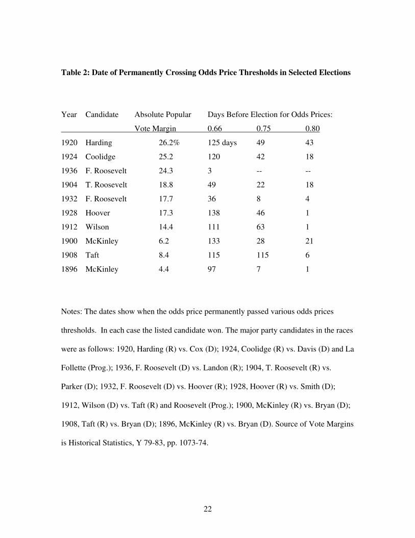
When an election would be decided by a wide margin, the betting markets were

generally successful in picking the winner early. Table 2 shows the dates when odds price

permanently passed various thresholds for selected presidential races. In many elections

decided by a wide margin, the odds price on the favorite started high and accelerated to

still higher levels as Election Day approached. This pattern is illustrated in Figure 3,

6

which compares the favorite’s odds price in the 1924 New York betting market with

those in the 1996 Iowa Electronic Markets Winner-Take-All contract.

Betting Prices as Information

Covering developments in the Wall Street betting market was a staple of election

reporting before World War Two. Prior to the innovative polling efforts of Gallup, Roper,

and Crossley, the other information available about future election outcomes was limited

to the results from early-season contests, overtly partisan canvasses, and straw polls of

unrepresentative and typically small samples. The largest and best-known non-scientific

survey was the Literary Digest poll (which tabulated millions of returned postcard ballots

that were mass mailed to a sample drawn from telephone directories and automobile

registries). After predicting the presidential elections correctly from 1916 to 1932, the

Digest famously called the 1936 contest for Landon in the election that F. Roosevelt won

by the largest Electoral College landslide of all time. Notably, although the Democrat’s

odds prices were relatively low in 1936, the betting market did pick the winner correctly

(see the third row of Table 2). The published price quotes allowed people who had not

followed the election to catch up immediately. As an example, when Andrew Carnegie

returned in late October 1904 from his annual vacation to Scotland, he stated at his arrival

press conference: “From what I see of the betting,…I do not think that Mr. Roosevelt will

need my vote. I am sure of his election… (New York Times, October 24, 1904 p. 1).”

The betting quotes filled the demand for accurate odds from a public widely

interested in wagering on elections. In this age before mass communication technologies

reached into America’s living rooms, election nights were highly social events,

7

comparable to New Year’s Eve or major football games. In large cities, crowds filled

restaurants, hotels, and sidewalks in downtown areas where newspapers and brokerage

houses would publicize the latest returns and people with sporting inclinations would

wager on the outcomes. Even for those who could not afford large stakes, betting in the

run-up to elections was a cherished ritual. A widely-held value was that one should be

prepared to “back one’s beliefs” either with money or more creative dares. Making freak

bets – where the losing bettor literally ate crow, pushed the winner around in a

wheelbarrow, or engaged in similar public displays– was wildly popular. Gilliams (1901,

p.186) offered “a moderate estimate” that in the 1900 election “there were fully a half-

million such [freak] bets—about one for every thirty voters.” In this environment, it is

hardly surprising that the leading newspapers kept their readership well informed about

the latest market odds.

Markets vs. Manipulation

Newspapers of this time couched their explanations of the accuracy of the Wall

Street betting odds with analogies to stock prices. The New York Times wrote on October

7, 1924 (p. 18) “The Wall Street odds represent the consensus of a large body of

extremely impartial opinion that talks with money and approaches Coolidge and Davis as

dispassionately as it pronounces judgment on Anaconda and Bethlehem Steel.” Similarly,

a few days later another article in the Times explained (October 10, 1924, p. E9):

Wall Street is always the place to which inside information comes on an election canvas … [and] it is a Wall Street habit, when risking a large amount of money, not to allow sentiment or partisanship to swerve judgments—an art learned in stock speculation; …any attempt to force

8

odds in a direction unwarranted by the facts will always instantly attract money to the opposite side, precisely as overvaluation of a stock on the market will cause selling and its under-valuation will attract buying.

In the 1920s and 1930s, when betting activity moved towards specialist firms, the

participants did not wait for political insiders to enter with private information, but

instead began to conduct their own market analysis. According to a 1924 Wall Street

Journal story (September 29, p. 13), the “betting firms maintain a statistical department

for the benefit of their customers and also have a man present at the principal speeches

made by the candidates. This man makes unbiased reports of the psychological reactions

of the audiences.” In 1936, according to the Washington Post (November 3, p. 16), upon

becoming suspicious of the results of the Literary Digest canvas, Sam Boston,

“American’s most distinguished betting commissioner,” began “conducting his own

election poll.”

At least two specific mechanisms could lead betting markets to aggregate

information appropriately. The first case involves well-informed betting commissioners

who serve as market makers and use their impartial beliefs to set the prices competitively.

The commissioners have incentive to participate despite an absence of profit-making

trades because they collect commissions. The second mechanism allows for partisan

bettors lacking aggregate information. If each voter placed a one-dollar bet for his

favorite candidate in a pari-mutuel, the betting totals would accurately pick the winner

(though the price would not typically equal the probability of winning).

Working against the market forces leading to information aggregation were

motivations to manipulate the odds for political gain. Given that the betting odds were

taken as good indicators of the candidate’s strength, the betting markets potentially

9

provided a lever for influencing expectations. The newspapers periodically contained

charges that partisans were manipulating the reported betting odds to create a bandwagon

effect. This could happen if the reported betting was only a “wash sale” between

confederates or it occurred outside the open market. Partisan newspapers also played a

role through selective reporting. The most common thinking was that pushing up odds

helped the preferred candidate by depressing the effort and turnout for the opposing

candidate. If the marginal bettor was a partisan, was influenced by a manipulation, or

received information from a biased source, the markets would systematically err in their

predictions.

The press did frequently refer to the betting activities of officials associated with

the Republican and Democratic National Committees, with state party organizations from

across the east, and especially with Tammany Hall (the New York City Democratic

machine). The newspapers recorded many betting and bluffing contests between Col.

Thomas Swords, Sergeant of Arms of the National Republican Party, and Democratic

betting agents representing Richard Croker, Boss of Tammany Hall, among others. In

most but not all instances, these officials appear to bet in favor of their party’s candidate;

in the few cases where they took the other side, it was typically to hedge earlier bets.

However, there are only a few minor instances where market manipulation

appears plausible. For example, in 1892 the Republican campaign managers went at

midnight to the Hoffman House (the Democratic hangout) offering to bet large stakes at

odds consistent with their candidate having a better than previously expected chances of

winning. Small fry, not the big Tammany money was around, so the offered large bets

10

were not taken. The odds quoted in the newspapers made the Republican candidate

appear stronger than he was (New York Times, November 8, 1892, p. 8).

Another barrier to accurate forecasts was the lack of national information sources.

Over most of this period, news spread by telegraphs and was first made public in

newspapers. As a result, news events might only slowly be reflected in prices. This effect

might also dampen the odds price on favorites because there was always the possibility of

latent bad news arriving. Also, since certain geographic areas received news later, a

possibility existed of traders from information-rich areas earning excess returns, a topic

we return to below.

One other potential friction did not prove to be problematic. The betting market

repeatedly had to confront elections that were not decided until long after the polls

closed. In the 1876 Hayes-Tilden race, the outcome was disputed for months after

Election Day with the political parties charging each other with fraudulently

manufacturing votes. A special Electoral Commission eventually resolved this hotly

contested election on a strict party-line vote. The acrimony spilled over into the betting

market, where John Morrissey, the leading New York pool-seller (where the winners

divide the total pool of money bet, minus the commission), opted to cancel the pools,

returning the stakes minus his commission. This solution while understandable left many

unsatisfied and contributed to the push in the next session of the New York legislature to

outlaw pool-selling. In later years, betting commissioners handled contested elections by

making the contracts contingent on whomever took office and by withholding payment

until one candidate officially conceded. Indeed, they often kept the betting action alive. In

the close 1884 election, betting lasted until the Friday after the election. In 1916, the

11

leading betting commissioners did not settle up until November 23, almost two weeks

after the polls closed. In the 1888 contest, when Harrison won the electoral college vote

outright (233-168) and yet Cleveland very narrowly won the popular vote, settlement in

favor of Harrison bettors occurred without a hitch.

Market Efficiency

In an efficient capital market, asset prices reflect all relevant information and thus

provide the best prediction of future events given the current information (Roll, 1984).

Because election bets paid on victory (a binary event), efficient prices in this market

should reflect the probabilities of the election outcomes. We now test whether the

election betting market satisfies a standard set of efficiency conditions: arbitrage-free

pricing, weak-, semistrong-, and strong-form efficiency (Fama, 1970). Efficiency tests

based on more structured models appear in Rhode and Strumpf (2004).

One of the weakest conditions for efficiency is arbitrage-free pricing, so that

participants cannot instantly profit from simultaneously trading some set of contracts. In

the context of election betting markets, the sum of the odds prices on all possible

candidates cannot differ from a dollar by more than commission costs. For example, if

the sum of prices on bets paying a dollar is strictly less than a dollar, then (abstracting

from commissions) a trader can guarantee a profit by purchasing one share of each

contract, since this ensures betting less than a dollar to win a dollar. We can evaluate this

hypothesis in those elections when we observe the prices for all distinct contracts, as in

1912, 1916, and 1924. The arbitrage-free condition holds in most such cases, but it is

12

violated for certain periods. For example, the Hughes and Wilson prices sum to less than

a dollar during eight days in the beginning of September 1916, and the Wilson,

Roosevelt, and Taft prices sum to more than a dollar for the ten days just prior to the

election in 1912. These differences are larger than the typical 5 percent commission rate,

making arbitrage possible. Still, such violations are rare. In only 25 out of 807

observations are the sums far enough from one dollar to allow arbitrage. Moreover, it is

unclear how many shares a participant could trade before altering the odds and

eliminating the possibility of arbitrage.

A related arbitraging condition is the law of one price. This states that prices at

different locations should be close enough, taking commission and transportation costs

into account, that investors cannot simultaneously buy and sell contracts for a profit. The

law of one price appears to hold for the various markets within New York City. Prices on

a given contact usually differed by no more than a tick, and different newspapers reported

virtually the same odds were available on a given day (when listings are available from

multiple newspapers, the correlation coefficient for the prices is 0.983 with N=344).

Cursory evidence indicates price variations across U. S. cities existed, but tended to be

small.3 We also know that investors actively worked to arbitrage pricing gaps and that at

least one betting commissioner maintained offices in both New York and Chicago

(Washington Post, November 1, 1932, p. 9).

A capital market is weak-form efficient if historical asset prices cannot be used to

devise profitable trading rules. A loose implication of weak-form efficiency is that it is

not possible to forecast prices using lagged price data, implying prices follow a random

3 As examples, a 1888 Chicago Tribune survey of 10 major cities on election eve revealed the coefficient of variation of the odds prices was only 5.1 percent (November 6, 1888, p. 3) and a similar New York World survey of 13 cities in 1916 have a coefficient of variation of 4.6 percent (November 7, 1916, p. 1).

13

walk. Consistent with this, we find it is not possible to reject the hypothesis that daily

odds prices follow a random walk in our 1884-1940 sample (N=236).4 Another test

considers whether price changes can be forecast using historical data. When we regress

the change in daily prices on its lags, the lagged prices do not have statistically significant

effects (N=120).5 These simple tests are broadly consistent with weak-form efficiency

and parallel results for the presidential betting markets in the Iowa Electronic Markets

(Berg et al., 2003).

A capital market satisfies semistrong-form efficiency if an investor cannot expect

to make excess returns based on publicly available information. A simple if low-powered

test is to examine whether one could use generally available information to devise a

betting rule that would yield profits above the commission costs. We experimented with

three simple rules involving buying a single contract paying one dollar on: 1) the

4 We estimate the equation, priceit = α + β×priceit-1 + uit where priceit is the price of some contract in election i occurring at day t and priceit-1 is a lag of price. The estimated β’s are 1.01, 1.01 and 0.99 for Democrat, Incumbent and Market Favorite party contracts, and these are statistically indistinguishable from unity (using classical or robust standard errors); the estimated α’s are each indistinguishable from zero. We find similar results for an AR(2) process. Note this approach may be misspecified because efficiently priced options with termination dates can have a deterministic drift. Intuitively, as Election Day approaches, uncertainty about the outcome is likely to diminish because more voters make up their minds and there are fewer opportunities for an “October surprise.” The favorite’s probability of victory (and thus his market price) increases to one—as illustrated in Figure 3-- while that of underdog falls to zero. After accounting for these effects, we still can not reject weak-form efficiency. See Rhode-Strumpf (2004) for a detailed theoretical and empirical treatment of this issue. 5 The equation we estimate is ∆priceit = β0 + β1×∆priceit-1 + β2×∆priceit-2 + uit where the variables are defined in the previous note. The estimated (β1, β2)’s are (-0.24, 0.14), (-0.26, 0.12) and (-0.20, 0.14) for Democrat, Incumbent and Market Favorite party contracts, and these are statistically indistinguishable from zero using robust standard errors. When just a single price lag is used, the estimated parameters are significantly negative. However, we find somewhat analogous results in analyzing the Democrat party contract for the Iowa Electronic Markets Winner-Take-All presidential market using daily price data from 1992, 1996, and 2000.

14

Democrat; 2) the market favorite; or 3) the party in power. We also consider the

alternative of betting one dollar (instead of buying one contract) on each of these choices,

which places more weight on long-shots. We found that buying one-dollar contracts on

the Democrats, favorites, and members of the incumbent party tended to be winning

strategies over the 1884-1940 period.6 However the positive returns are not at all robust.

The winning strategies typically yielded small net returns relative to their standard

deviations. Moreover, strategies that made money in the first half of the time period (such

as betting against the favorite) often lost in the second half of the time period. Some

choices made money in the form of betting one dollar, but not in the form of buying one

contract, or vice versa. These results, as well as the more formal tests reported in Rhode

and Strumpf (2004), suggest that it was difficult to use public information to construct a

winning betting strategy. Again the modern Iowa Electronic Market provides a useful

benchmark. For the 1992-2000 period, we found that its Winner-Take-All bets allowed

similar profitable opportunities– although this result should be viewed with caution given

the small number of elections in the Iowa data.

Finally, we consider strong-form efficiency, which involves whether an investor

can earn excess profits using private information. While this hypothesis is difficult to

quantify, there are several reports of insiders profiting from superior information about

specific states. In 1916, for example, some west coast investors wagered heavily on

Wilson because they believed he would achieve an upset win in California, which he did 6 The result for favorites is of interest since it suggests the possibility that markets did not place a high enough probability on the favorite which is consistent with the favorite-long shot bias observed in racetrack betting (Thaler and Ziemba, 1988). One explanation for this finding is the role of commissions when one party is the heavy favorite. Suppose the Democrats are known to be more than 95 percent likely to win a contest. A bookmaker cannot offer these objective odds because the bettors will not be able to overcome the standard 5 percent commission. Hence, market odds must be biased down in such extreme election cases. The result concerning the under-pricing of Democrats might reflect the influence of wealthier, partisan Republican bettors.

15

(Wall Street Journal, October 31, 1916, p. 8). Leveraging on superior local information,

several Ohioans fronted by the famous New York boxing promoter Tex Rickard (who

was the main force behind the building of Madison Square Garden) placed a $60,000

wager on Wilson to win their state (New York Times, Oct. 28, 1916, p. 1). These beliefs

must have been strong ones since the wager moved the odds price by nearly ten

percentage points, and again the investors proved correct. It seems that insiders were able

to profit from their information advantage, but rejections of strong efficiency are typical

of most capital markets.

In conclusion, the historical betting markets do not meet all of the exacting

conditions for efficiency, but the deviations were not usually large enough to generate

consistently profitable betting strategies using public information.7 The performance of

the market was comparable to its modern counterparts and, given the barriers to

efficiency discussed earlier, quite remarkable.

The Decline of Political Wagering

The newspapers reported substantially less betting activity in specific contests and

especially after 1940. In part, this reduction in reporting reflected a growing reluctance of

newspapers to give publicity to activities that many considered unethical. There were

frequent complaints that election betting was immoral and contrary to republican values.

7 The wager markets on state election outcomes over this time period more convincingly fail the efficiency conditions. Rhode and Strumpf (2004) devise various profitable betting strategies based on public information. This result is unsurprising given that the state markets were far thinner than the national market.

16

Among the issues critics raised were moral hazard, election tampering, information

withholding, and strategic manipulation.8

In response to such concerns, New York state laws did increasingly attempt to

limit organized election betting. Casual bets between private individuals always remained

legal in New York. However, even an otherwise legal private bet on elections technically

disqualified the participants from voting – although this provision was rarely enforced --

and the legal system also discouraged using the courts to collect gambling debts. Anti-

gambling laws passed in New York during the late 1870s and the late 1900s appear to put

a damper on election betting, but in both cases the market bounced back after the energy

of the moral reformers flagged. Ultimately, New York’s legalization of pari-mutuel

betting on horse races in 1939 may have done more to reduce election betting than any

anti-gambling policing. With horse-racing, individuals interested in gambling now had

several contests per day to wager on that promised immediate rewards rather than a

single, long political contest.

New York State was not alone in changing the legal and regulatory environment

for election betting activity. The New York Stock Exchanges and the Curb Market also

periodically tried to crack down. The exchanges characteristically did not like the public

to associate their socially productive risk-sharing and risk-taking functions with gambling

on inherently zero-sum sporting events. In the 1910s and again after the mid-1920s, the

stock exchanges passed regulations to reduce the public involvement of their members. In

May 1924, for example, both the New York Stock Exchange and the Curb Market passed

resolutions expressly barring their members from engaging in election gambling. Activity

8 For selected historical criticisms of election betting, see New York Tribune, Nov. 18, 1888, p. 6; New York Times, Oct. 28, 1896, p. 1; Nov. 3, 1896, p. 2; Washington Post, Oct. 28, 1912, p. 2. For a recent discussion, see Hanson (2003).

17

continued to be reported in the newspapers, but now the articles rarely named the

participants. During the 1930s, the press noted that securities of private electrical utilities

had effectively become wagers on Roosevelt (which makes sense because New Deal

policy initiatives such as SEC and TVA constrained the profits of utilities).

A final force pushing election betting underground was the rise of scientific

polling. For newspapers, one of the functions of reporting Wall Street betting odds had

been to provide the best available aggregate information. Following the success of Gallup

in predicting the 1936 election, many newspapers stopped lending credence to the

Literary Digest poll. The scientific polls, available on a weekly basis, provided the media

with a ready substitute for the betting odds, one not subject to the moral objections

against gambling. Our survey of the Washington Post and New York Times indicates that

articles on the Literary Digest poll began to out-number those on election betting in 1924

and 1928, respectively. Articles related to the Gallup poll began to appear in 1936 and to

outnumber those in the other two categories by 1940. Whatever election betting which

continued to occur received far less media attention.

Lessons for the Future

Wagering on presidential elections has a long tradition in the United States, with

large and often well-organized markets operating for over three-quarters of a century

before the Second World War. The resulting betting odds proved remarkably prescient

and almost always correctly predicted election outcomes well in advance, despite the

absence of scientific polls. This historical experience suggests a promising role for other

prediction markets. Our analysis complements a substantial body of experimental

18

research which has hinted that asset markets can successfully aggregate information

(Forsythe, et al., 1982; Plott and Sunder, 1988). The informational efficiency of

prediction markets has also been investigated in the field, such as Camerer’s (1998) study

of the difficulty of manipulating racetrack pari-mutuels and Leigh et al.’s (2003) study of

futures markets on war probabilities.

However, recent experience indicates public skepticism about applying markets to

novel situations. In summer 2003, word leaked out that the Department of Defense was

considering setting up a Policy Analysis Market, somewhat similar to the Iowa Electronic

Market, which would seek to provide a market consensus about international political

developments, especially in the Middle East. Critics argued that this market was subject

to manipulation by insiders and might allow extremists to profit financially from their

actions. But these concerns were also evident in the historical wagering on presidential

elections, with partisans serving as active participants and contemporary fears of election

tampering. Although large sums of money were at stake in the historical presidential

betting markets, we are not aware of any evidence that the political process was seriously

corrupted by the presence of a wagering market. There are obviously important

differences between the proposed Policy Analysis Market and the New York betting

market, but the experience described in this paper suggests that many current concerns

about the appropriateness of prediction markets are not well founded in the historical

record.

19

Acknowledgements

We thank Patrick Conway, Lee Craig, Thomas Geraghty, James Hines, Thomas

Mroz, Mark Stegeman, Timothy Taylor, Michael Waldman, and Justin Wolfers for

comments and suggestions.

20

References

Berg, Joyce, Forrest Nelson and Thomas Rietz (2003). “Accuracy and Forecast Standard Error of Prediction Markets.” University of Iowa working paper. Camerer, Colin (1998) “Can Asset Markets be Manipulated? A Field Experiment with Racetrack Betting.” Journal of Political Economy. 106:457-82. Fama, Eugene (1970). “Efficient Capital Markets: A Review of Theory and Empirical Work.” Journal of Finance. 25: 383-417. Forsythe, Robert, Thomas Palfrey, and Charles Plott (1982). “Asset Valuation in an Experimental Market.” Econometrica. 50: 537-568. Gilliams, E. Leslie (1901). “Election Bets in America” Strand Magazine. XXI: 185-191. Hanson, Robin (2003) “Shall We Vote Values, But Bet of Beliefs?” (Sept.) George Mason working paper. Leigh, Andrew, Justin Wolfers and Eric Zitzewitz (2003). “What Do Financial Markets Think of War in Iraq?” NBER working paper 9587. Plott, Charles, and Shyam Sunder (1988). “Rational Expectations and the Aggregation of Diverse Information in Laboratory Security Markets.” Econometrica. 56: 1085-1118. Rhode, Paul, and Koleman Strumpf (2004). “Historical Prediction Markets: Wagering on Presidential Elections.” working paper. Roll, Richard (1984). “Orange Juice and Weather.” American Economic Review. 74: 861-880. Thaler, Richard and William Ziemba (1988). “Parimutuel Betting Markets: Racetracks and Lotteries.” Journal of Economic Perspectives. Spring (2:2) 161-174. Thoreau, Henry David (1967). The Variorum Civil Disobedience. New York: Twayne.

21

Table 1: New York Election Betting Volume

New York Betting Volume 2002 dollars Dollars per Dollars per (millions) Votes Cast Campaign Spending

1884 13.7 1.36 0.278 1888 37.6 3.30 0.907 1892 14.8 1.23 0.185 1896 10.7 0.77 0.124 1900 63.9 4.57 0.876 1904 50.3 3.72 0.894 1908 7.7 0.52 0.174 1912 4.6 0.30 0.087 1916 165.0 8.90 2.116 1920 44.9 1.68 0.726 1924 21.0 0.72 0.373 1928 10.5 0.29 0.086

Average 37.0 2.28 0.532

Notes: These figures report newspaper estimates of total bet volume over the course of

the election cycle. See Rhode and Strumpf (2004) for details.

22

Table 2: Date of Permanently Crossing Odds Price Thresholds in Selected Elections

Year Candidate Absolute Popular Days Before Election for Odds Prices:

Vote Margin 0.66 0.75 0.80

1920 Harding 26.2% 125 days 49 43

1924 Coolidge 25.2 120 42 18

1936 F. Roosevelt 24.3 3 -- --

1904 T. Roosevelt 18.8 49 22 18

1932 F. Roosevelt 17.7 36 8 4

1928 Hoover 17.3 138 46 1

1912 Wilson 14.4 111 63 1

1900 McKinley 6.2 133 28 21

1908 Taft 8.4 115 115 6

1896 McKinley 4.4 97 7 1

Notes: The dates show when the odds price permanently passed various odds prices

thresholds. In each case the listed candidate won. The major party candidates in the races

were as follows: 1920, Harding (R) vs. Cox (D); 1924, Coolidge (R) vs. Davis (D) and La

Follette (Prog.); 1936, F. Roosevelt (D) vs. Landon (R); 1904, T. Roosevelt (R) vs.

Parker (D); 1932, F. Roosevelt (D) vs. Hoover (R); 1928, Hoover (R) vs. Smith (D);

1912, Wilson (D) vs. Taft (R) and Roosevelt (Prog.); 1900, McKinley (R) vs. Bryan (D);

1908, Taft (R) vs. Bryan (D); 1896, McKinley (R) vs. Bryan (D). Source of Vote Margins

is Historical Statistics, Y 79-83, pp. 1073-74.

23

Figure 1: Democratic Odds Price and Popular Vote Margin, 1884-1940

Dem

ocra

tic O

dds

Pric

es

Dem. Popular Vote Margin

<Year>= Odds 1-15 Days =Cubic Fit 1-15 Days Year = Odds 31-45 Days =Cubic Fit 31-45 Days

-.25 -.125 0 .125 .25

0

.2

.4

.6

.8

<1920><1920><1920><1920><1920><1920><1920><1920><1920><1920><1920><1920><1920><1920><1920><1920><1920><1920><1920><1920><1920><1920><1920><1920><1920><1920><1920><1920><1920><1920><1920><1920><1920><1920><1920><1920><1920><1920><1920><1920><1920><1920><1920><1920><1920><1920><1920><1920><1920><1920>

<1924><1924><1924><1924><1924><1924><1924><1924><1924><1924><1924><1924><1924><1924><1924><1924><1924><1924><1924><1924><1924><1924><1924><1924><1924><1924><1924><1924><1924><1924><1924><1924><1924><1924><1924><1924><1924><1924><1924><1924><1924><1924><1924><1924><1924><1924><1924><1924><1924><1924><1924><1924><1924><1924><1924><1924><1924><1924><1924><1924><1924><1924><1924><1924><1924><1924><1924><1924><1924><1924><1924><1924><1924><1924><1924><1924><1924><1924><1924><1924><1924><1924><1924><1924><1924><1924><1924><1924><1924><1924><1924><1924>

<1904><1904><1904><1904><1904><1904><1904><1904><1904><1904><1904><1904><1904><1904><1904><1904><1904><1904><1904><1904><1904><1904><1904><1904><1904><1904><1904><1904><1904><1904><1904><1904><1904><1904><1904><1904><1904><1904><1904><1904><1904><1904><1904><1904><1904><1904><1904><1904><1904><1904><1904><1904><1904><1904><1904><1904><1904><1904><1904><1904><1904><1904><1904><1904><1904><1904><1904><1904><1904><1904><1904><1904><1904><1904><1904><1904><1904><1904><1904><1904><1904><1904><1904><1904><1904><1904><1904><1904><1904><1904><1904><1904><1904><1904><1904><1904><1904><1904><1904><1928><1928><1928><1928><1928><1928><1928><1928><1928><1928><1928><1928><1928><1928><1928><1928><1928><1928><1928><1928><1928><1928><1928><1928><1928><1928><1928><1928><1928><1928><1928><1928><1928><1928><1928><1928><1928><1928><1928><1928><1928><1928><1928>

<1908><1908><1908><1908><1908><1908><1908><1908><1908><1908><1908><1908><1908><1908><1908><1908><1908><1908><1908><1908><1908><1908><1908><1908><1908><1908><1908><1908><1908><1908><1908><1908><1908><1908><1908><1908><1908><1908><1908><1908><1908><1908><1908><1900><1900><1900><1900><1900><1900><1900><1900><1900><1900><1900><1900><1900><1900><1900><1900><1900><1900><1900><1900><1900><1900><1900><1900><1900><1900><1900><1900><1900><1900><1900><1900><1900><1900><1900><1900><1900><1900><1900><1900><1900><1900><1900><1900><1900><1900><1900><1900><1900><1900><1900><1900><1900><1900><1900><1900><1900><1900><1900><1900><1900><1900><1900><1900><1900><1900><1900><1900><1900><1900><1900><1900><1900><1900><1900><1900><1900><1900><1900><1900><1900><1900>

<1896><1896><1896><1896><1896><1896><1896><1896><1896><1896><1896><1896><1896><1896><1896><1896><1896><1896><1896><1896><1896><1896><1896><1896><1896><1896><1896><1896><1896><1896><1896><1896><1896><1896><1896><1896><1896><1896><1896><1896><1896><1896><1896><1896><1896><1896><1896><1896><1896><1896><1896><1896><1896><1896><1896><1896>

<1884><1884><1884><1884><1884><1884><1884><1884><1884><1884><1884><1884><1884><1884>

<1888><1888><1888><1888><1888><1888><1888><1888><1888><1888><1888><1888><1888><1888><1888><1888><1888><1888><1888><1888><1888><1888><1888><1888><1888><1888><1888><1888><1888><1888><1888><1888><1888><1888><1888><1888><1888><1888><1888><1888><1892><1892><1892><1892><1892><1892><1892><1892><1892><1892><1892><1892><1892><1892><1892><1892><1892><1892><1892><1892><1892><1892><1892><1892><1892><1892><1892><1892><1892><1892><1892><1892><1892><1892><1892><1892><1892><1892><1892><1892><1892><1892><1892><1892><1892><1892><1892><1892>

<1916><1916><1916><1916><1916><1916><1916><1916><1916><1916><1916><1916><1916><1916><1916><1916><1916><1916><1916><1916><1916><1916><1916><1916><1916><1916><1916><1916><1916><1916><1916><1916><1916><1916><1916><1916><1916><1916><1916><1916><1916><1916><1916><1916><1916><1916><1916><1916><1916><1916><1916><1916><1916><1916><1916><1916><1916><1916><1916><1916><1916><1916><1916><1916><1916><1916><1916><1916><1916><1916><1916><1916><1916><1916><1916><1916><1916><1916><1916><1916><1916><1916><1916><1916><1916><1916><1916><1916><1916><1916><1916><1916><1916><1916><1916><1916><1916><1916><1916><1916><1916><1916><1916><1916><1916><1916><1916><1916><1916><1916><1916><1916><1916><1916><1916><1916><1916><1916><1916><1916><1916><1916><1916><1916><1916><1916><1916><1916><1916><1916><1916><1916><1916><1916><1916><1916><1916><1916><1916><1916><1916><1916><1916><1916><1916><1916><1916><1916><1916><1916><1916><1916><1916><1916>

<1940><1940><1940><1940><1940><1940><1940><1940><1940><1940><1940><1940><1940><1940><1940><1940><1940><1940><1940><1940><1940>

<1912><1912><1912><1912><1912><1912><1912><1912><1912><1912><1912><1912><1912><1912><1912><1912><1912><1912><1912><1912><1912><1912><1912><1912><1912><1912><1912><1912><1912><1912><1912><1912><1912><1912><1912><1912><1912><1912><1912><1912><1912><1912><1912><1912><1932><1932><1932><1932><1932><1932><1932><1932><1932><1932><1932><1932><1932><1932><1932><1932><1932><1932><1932><1932><1932><1932><1932><1932>

<1936><1936><1936><1936><1936><1936><1936><1936><1936><1936><1936><1936><1936><1936><1936><1936><1936><1936><1936><1936><1936><1936><1936><1936><1936><1936><1936><1936><1936><1936><1936><1936><1936><1936><1936><1936><1936><1936><1936><1936><1936><1936><1936><1936><1936>

19201920192019201920192019201920192019201920192019201920192019201920192019201920192019201920192019201920192019201920192019201920192019201920192019201920192019201920192019201920192019201920192019201920

19241924192419241924192419241924192419241924192419241924192419241924192419241924192419241924192419241924192419241924192419241924192419241924192419241924192419241924192419241924192419241924192419241924192419241924192419241924192419241924192419241924192419241924192419241924192419241924192419241924192419241924192419241924192419241924192419241924192419241924192419241924

190419041904190419041904190419041904190419041904190419041904190419041904190419041904190419041904190419041904190419041904190419041904190419041904190419041904190419041904190419041904190419041904190419041904190419041904190419041904190419041904190419041904190419041904190419041904190419041904190419041904190419041904190419041904190419041904190419041904190419041904190419041904190419041904190419041904

19281928192819281928192819281928192819281928192819281928192819281928192819281928192819281928192819281928192819281928192819281928192819281928192819281928192819281928192819281900190019001900190019001900190019001900190019001900190019001900190019001900190019001900190019001900190019001900190019001900190019001900190019001900190019001900190019001900190019001900190019001900190019001900190019001900190019001900190019001900190019001900190019001900190019001900190019001900190019001900190019001900190019001900

18961896189618961896189618961896189618961896189618961896189618961896189618961896189618961896189618961896189618961896189618961896189618961896189618961896189618961896189618961896189618961896189618961896189618961896189618961896

18841884188418841884188418841884188418841884188418841884

1888188818881888188818881888188818881888188818881888188818881888188818881888188818881888188818881888188818881888188818881888188818881888188818881888188818881888

189218921892189218921892189218921892189218921892189218921892189218921892189218921892189218921892189218921892189218921892189218921892189218921892189218921892189218921892189218921892189218921892

1916191619161916191619161916191619161916191619161916191619161916191619161916191619161916191619161916191619161916191619161916191619161916191619161916191619161916191619161916191619161916191619161916191619161916191619161916191619161916191619161916191619161916191619161916191619161916191619161916191619161916191619161916191619161916191619161916191619161916191619161916191619161916191619161916191619161916191619161916191619161916191619161916191619161916191619161916191619161916191619161916191619161916191619161916191619161916191619161916191619161916191619161916191619161916191619161916191619161916191619161916191619161916

194019401940194019401940194019401940194019401940194019401940194019401940194019401940

19121912191219121912191219121912191219121912191219121912191219121912191219121912191219121912191219121912191219121912191219121912191219121912191219121912191219121912191219121912

193219321932193219321932193219321932193219321932193219321932193219321932193219321932193219321932193619361936193619361936193619361936193619361936193619361936193619361936193619361936193619361936193619361936193619361936193619361936193619361936193619361936193619361936193619361936

Note: The vertical axis is the average market odds over some period, and the horizontal

axis is the actual vote outcome. The regressions and averages are based on 417

observations of betting quotes for the period 1-15 days before the election and 65

observations for period 31-45 days before.

24

Figure 2: Comparing 1916 and 2000 Elections

Panel A: New York Market for 1916 Election O

dds

Pric

e

Days Until Election

DemPrice_1916

150 120 90 60 30 0

0

.25

.5

.75

1

Panel B: IEM Data for 2000 Election

Odd

s P

rice

(WTA

mar

ket)

Days Until Election

DemPrice_2000

150 120 90 60 30 0

0

.25

.5

.75

1

25

Figure 3: Comparing the 1924 and 1996 Elections

Panel A: NY Market for 1924 Election

Odd

s P

rice

Days Until Election

Rep Price 1924

120 100 80 60 40 20 0

.5

.75

1

Panel B: IEM Data for 1996 Election

Odd

s P

rice

(WTA

mar

ket)

Days Until Election

DemPrice_1996

120 100 80 60 40 20 0

.5

.75

1