Historical Prediction Markets:

Wagering on Presidential Elections*

Paul W. Rhode** Koleman S. Strumpf UNC Chapel Hill and NBER UNC Chapel Hill

November 2003

* We thank Thomas Mroz, Mark Stegeman, and Justin Wolfers for comments and suggestions. **Corresponding author. UNC Chapel Hill, Department of Economics, CB# 3305, Chapel Hill NC 27599. email: prhode@email.unc.edu.

1

I: Introduction

Interest in using markets to forecast non-financial outcomes has grown with the

rising popularity of internet wagering and the proposed establishment of a terrorism

futures exchange. While many treat such prediction markets as recent phenomena,

wagering on political outcomes has a long tradition in the United States. This paper

analyzes the large and often well-organized markets for betting on presidential elections

that operated between 1868 and 1940. Over $165 million (in 2002 dollars) was wagered

in one election, and betting activity at times dominated transactions on the stock

exchanges on Wall Street.

Drawing on an investigation of several thousand newspaper articles, we address

four main points. First, the market did an admirable job in forecasting elections in a

period before scientific polling. In only one case did the candidate clearly favored in the

betting a month before Election Day lose, and even state-specific forecasts were quite

accurate. This performance compares favorably with that in the Iowa Electronic Market

(IEM), the modern incarnation of this market. Second, we argue that several factors

work against generating accurate forecasts, such as the limited information of participants

and attempts to manipulate the odds by political parties and newspapers. Nonetheless,

we show that, based on an analysis of a daily time series of odds, the market passed

several (but not all) formal tests of efficiency. It was difficult to devise strategies leading

to excess profits. The market also managed to overcome shocks such as changes in the

legality of wagering, disputed elections, and surprising late returns. Third, we speculate

that political betting markets disappeared largely because of the rise of scientific polls

and the increasing availability of other forms of gambling. Finally, we argue that this

experience provides lessons for the present. It adds to the largely experimental body of

work that suggests that such markets are likely to be a useful tool in aggregating

information about events in which markets are typically ignored. And in opposition to

long-standing concerns, there is little evidence in the historical record that wagering

compromised the integrity of elections despite the active involvement of political parties.

2

II: Size and Scope of Historical Betting Markets

In the recent debates over prediction markets, one pertinent piece of history has

been all but forgotten: a large, active, and highly public market for betting on presidential

elections existed over much of US history before the Second World War. 1

Contemporaries noted this activity dated back to the election of Washington and existed

in organized markets (such as financial exchanges and pool-rooms) since the

administration of Lincoln. Although election betting was often illegal, the activity was

openly conducted by “betting commissioners” and employed standardized contracts that

promised a fixed dollar payment if the designated candidate won office. At times in the

late 19th and early 20th centuries, betting on political outcomes at the Curb Exchange in

New York would exceed trading in stocks and bonds.2 Crowds formed at the stock

exchanges – on the Curb or in the lobby of the NY Stock Exchange—and brokers would

call out bid-and-ask odds as if trading securities. In contests such as 1896, 1900, 1904,

1916, and 1924, the New York Times, Sun, and World provided nearly daily quotes from

early October until Election Day.3 On selected occasions, odds on winning each state

1 The organization and location of the New York betting market evolved over time. Moving out of pool-rooms in the 1880s, activity centered on the Curb Exchange and the major Broadway hotels until the mid-1910s. In the 1920s and 1930s, specialist firms of betting commissioners, operating out of offices on Wall Street, took over the trade. These firms were variously viewed as brokerages, bucket shops, or bookie joints. And whereas in the 1890s and early 1910s, the names and relatively modest (4-figure) stakes of bettors filled the daily newspapers, by the 1930s most of the reported wagering involved large (6-figure) amounts advanced by unnamed leaders in business or entertainment worlds. Undoubtedly, most of the activity occurred outside of our view.

The standard betting and commission structure over most of the period was for the betting commissioner to hold the stakes of both parties and charge a 5 percent commission on the winnings. If the commissioner trusted the credit-worthiness of the bettors, it was not always necessary to actually front the stakes and instead the signed memorandum or letter of obligation sufficed. New York Times, 10 Nov. 1906, p. 1; 29 May 1924, p. 21; 4 Nov. 1924, p. 2; Wall Street Journal, 29 Sept. 1924, p. 13. (At times such as in 1916, the commissioner apparently collected 2 percent from each side. New York Times, 9 Nov. 1916, p. 3) For the long tradition of election betting, see New York Herald Tribune, 2 Nov. 1940, p. 23. 2 As examples, see Chicago Tribune, 6 Nov. 1888, p. 2; New York Times, 4 Nov. 1896, p. 6; 8 Nov. 1898, p. 7; 10 Nov. 1916, p. 22; New York Tribune, 4 Nov. 1884, p. 10, 9 Nov. 1904, p. 2; 7 Nov. 1916, p. 1; Wall Street Journal, 7 Nov. 1916, p. 2. 3 The research in this paper has benefited substantially from a recent research innovation, the ability to search and access (via Proquest) machine-readable editions of historical newspapers including the New York Times, Wall Street Journal, and Washington Post. (Roughly one-half of our citations were found using old-fashioned microfilm and one-half using the new computer search engine.) Our prediction is these new search techniques will revolutionize the ability of scholars to access diffuse, qualitative information of phenomena such as election betting. A number of popular sources mention the existence of election betting—see, for example, Pietrusza (2003) p. 5 and Morris (2001) pp. 714-15 -- but we have found no study fully exploring this phenomenon.

3

were reported.4 While the New York market was the center of national betting activity,

similar markets emerged in Philadelphia, Chicago, Baltimore, and most other major

cities. 5

Compared to modern information markets, the volume of activity in the New

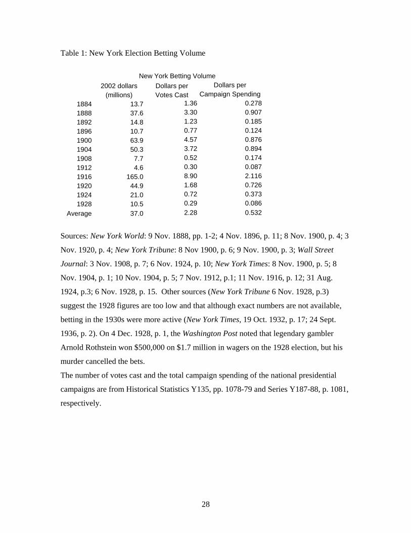
York betting market was astonishingly large. Table 1 assembles newspaper estimates,

converted to 2002 dollars, of the sums wagered in the New York market in the

presidential election years from 1884 to 1928. To provide firmer points of reference, the

table also shows the totals bet divided by the number of votes cast and the total spending

of the national presidential campaigns. The betting volume varied depending on the

closeness of the races, enthusiasm for the candidates, and the legal environment. The

1916 election was the high point, with some $165 million (2002 dollars) wagered in the

organized New York markets. This was more than twice the total spending on the

election campaigns. On average over this entire period, $37 million was wagered per

election. As a point of contrast, activity on the IEM for the 1988-2000 elections has been

orders of magnitude smaller, with trading volumes that never exceeded $0.15 million in

any one election (see Berg, et al, 2003).

III: Predictive Power of the “Wall Street Betting Odds”

The New York betting markets were widely recognized for their remarkable

ability to predict election outcomes. As the New York Times put it, the “old axiom in the

financial district [is] that Wall Street betting odds are ‘never wrong’ (28 Sept 1924, p.

4 There was also significant waging on the state vote pluralities in presidential contests and on state and local races, which typically took place in off-years. 5 There was also active betting on the American elections in London in elections such as 1896 (New York Times, 4 Nov. 1896, p. 6). Following the passage of anti-gambling legislation in New York in the 1908, Lloyds of London began offering insurance policies against the election of the Democrat, W. J. Bryan (New York Times, 18 July 1908, p. 14; 26 July 1908, p. SM9; 31 July 1908 p. 1). Such policies were expensive, however, and required proof of harm. It appears few if any policies were actually issued in 1908 or later years. According to the Wall Street Journal, (14 Oct. 1964, p. 1) the British bookmaking firm, Ladbroke and Co., did enter the election betting market on a serious basis in the mid-1960s.

4

E1).”6 The contemporary press noted that the Wall Street betting favorite almost always

won, the only exception being in 1916 when betting initially favored the eventual loser

(Hughes) but swung to even odds by the time the polls closed.

Indeed, in the 15 elections between 1884 and 1940, the mid-October betting

favorite won 11 times (73 percent) and the underdog won only once (Wilson in 1916). In

the remaining three contests (1884-92), the odds were essentially even and the races very

close. The ability of the betting market to aggregate information is all the more

remarkable given the absence of scientific polls before the mid-1930s. The betting odds

possessed much better predictive power than other generally available information such

as party affiliation or incumbency. Even if one takes the conservative assumption that

the 1884-92 predictions were failures, the New York betting record was more than a

match to chance.7

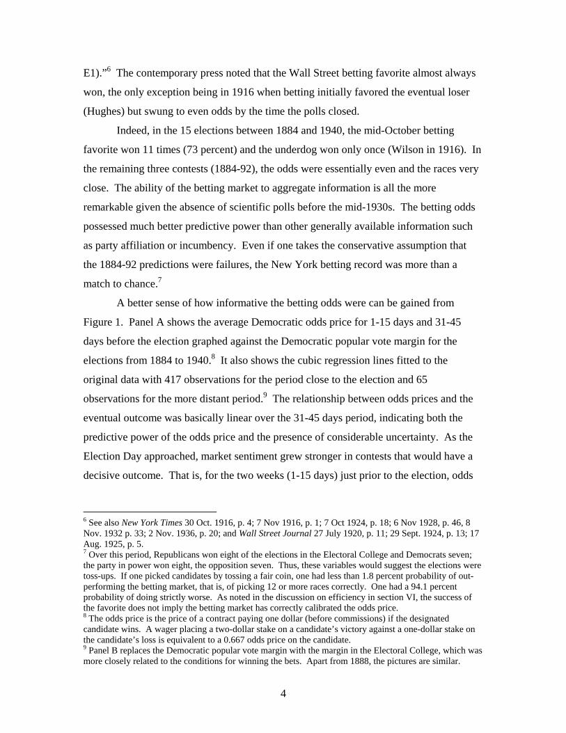
A better sense of how informative the betting odds were can be gained from

Figure 1. Panel A shows the average Democratic odds price for 1-15 days and 31-45

days before the election graphed against the Democratic popular vote margin for the

elections from 1884 to 1940.8 It also shows the cubic regression lines fitted to the

original data with 417 observations for the period close to the election and 65

observations for the more distant period.9 The relationship between odds prices and the

eventual outcome was basically linear over the 31-45 days period, indicating both the

predictive power of the odds price and the presence of considerable uncertainty. As the

Election Day approached, market sentiment grew stronger in contests that would have a

decisive outcome. That is, for the two weeks (1-15 days) just prior to the election, odds

6 See also New York Times 30 Oct. 1916, p. 4; 7 Nov 1916, p. 1; 7 Oct 1924, p. 18; 6 Nov 1928, p. 46, 8 Nov. 1932 p. 33; 2 Nov. 1936, p. 20; and Wall Street Journal 27 July 1920, p. 11; 29 Sept. 1924, p. 13; 17 Aug. 1925, p. 5. 7 Over this period, Republicans won eight of the elections in the Electoral College and Democrats seven; the party in power won eight, the opposition seven. Thus, these variables would suggest the elections were toss-ups. If one picked candidates by tossing a fair coin, one had less than 1.8 percent probability of out-performing the betting market, that is, of picking 12 or more races correctly. One had a 94.1 percent probability of doing strictly worse. As noted in the discussion on efficiency in section VI, the success of the favorite does not imply the betting market has correctly calibrated the odds price. 8 The odds price is the price of a contract paying one dollar (before commissions) if the designated candidate wins. A wager placing a two-dollar stake on a candidate’s victory against a one-dollar stake on the candidate’s loss is equivalent to a 0.667 odds price on the candidate. 9 Panel B replaces the Democratic popular vote margin with the margin in the Electoral College, which was more closely related to the conditions for winning the bets. Apart from 1888, the pictures are similar.

5

became much less favorable for the Democrat in elections he eventually lost by a non-

trivial margin and more favorable in those won by a non-trivial margin.

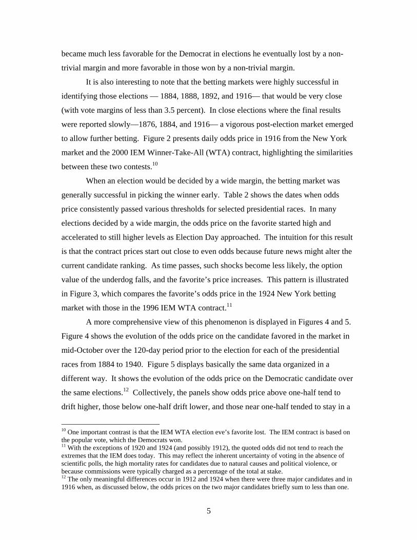
It is also interesting to note that the betting markets were highly successful in

identifying those elections — 1884, 1888, 1892, and 1916— that would be very close

(with vote margins of less than 3.5 percent). In close elections where the final results

were reported slowly—1876, 1884, and 1916— a vigorous post-election market emerged

to allow further betting. Figure 2 presents daily odds price in 1916 from the New York

market and the 2000 IEM Winner-Take-All (WTA) contract, highlighting the similarities

between these two contests.10

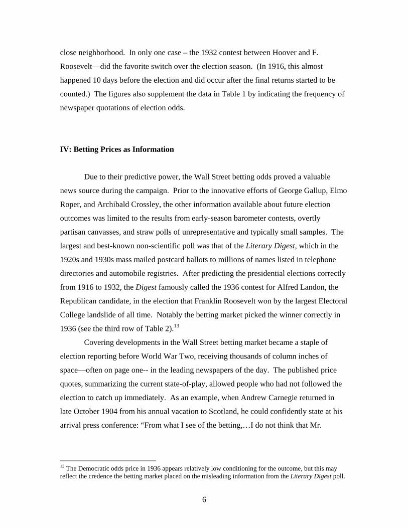
When an election would be decided by a wide margin, the betting market was

generally successful in picking the winner early. Table 2 shows the dates when odds

price consistently passed various thresholds for selected presidential races. In many

elections decided by a wide margin, the odds price on the favorite started high and

accelerated to still higher levels as Election Day approached. The intuition for this result

is that the contract prices start out close to even odds because future news might alter the

current candidate ranking. As time passes, such shocks become less likely, the option

value of the underdog falls, and the favorite’s price increases. This pattern is illustrated

in Figure 3, which compares the favorite’s odds price in the 1924 New York betting

market with those in the 1996 IEM WTA contract.11

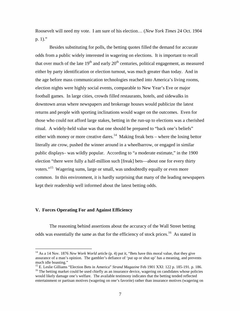
A more comprehensive view of this phenomenon is displayed in Figures 4 and 5.

Figure 4 shows the evolution of the odds price on the candidate favored in the market in

mid-October over the 120-day period prior to the election for each of the presidential

races from 1884 to 1940. Figure 5 displays basically the same data organized in a

different way. It shows the evolution of the odds price on the Democratic candidate over

the same elections.12 Collectively, the panels show odds price above one-half tend to

drift higher, those below one-half drift lower, and those near one-half tended to stay in a

10 One important contrast is that the IEM WTA election eve’s favorite lost. The IEM contract is based on the popular vote, which the Democrats won. 11 With the exceptions of 1920 and 1924 (and possibly 1912), the quoted odds did not tend to reach the extremes that the IEM does today. This may reflect the inherent uncertainty of voting in the absence of scientific polls, the high mortality rates for candidates due to natural causes and political violence, or because commissions were typically charged as a percentage of the total at stake. 12 The only meaningful differences occur in 1912 and 1924 when there were three major candidates and in 1916 when, as discussed below, the odds prices on the two major candidates briefly sum to less than one.

6

close neighborhood. In only one case – the 1932 contest between Hoover and F.

Roosevelt—did the favorite switch over the election season. (In 1916, this almost

happened 10 days before the election and did occur after the final returns started to be

counted.) The figures also supplement the data in Table 1 by indicating the frequency of

newspaper quotations of election odds.

IV: Betting Prices as Information

Due to their predictive power, the Wall Street betting odds proved a valuable

news source during the campaign. Prior to the innovative efforts of George Gallup, Elmo

Roper, and Archibald Crossley, the other information available about future election

outcomes was limited to the results from early-season barometer contests, overtly

partisan canvasses, and straw polls of unrepresentative and typically small samples. The

largest and best-known non-scientific poll was that of the Literary Digest, which in the

1920s and 1930s mass mailed postcard ballots to millions of names listed in telephone

directories and automobile registries. After predicting the presidential elections correctly

from 1916 to 1932, the Digest famously called the 1936 contest for Alfred Landon, the

Republican candidate, in the election that Franklin Roosevelt won by the largest Electoral

College landslide of all time. Notably the betting market picked the winner correctly in

1936 (see the third row of Table 2).13

Covering developments in the Wall Street betting market became a staple of

election reporting before World War Two, receiving thousands of column inches of

space—often on page one-- in the leading newspapers of the day. The published price

quotes, summarizing the current state-of-play, allowed people who had not followed the

election to catch up immediately. As an example, when Andrew Carnegie returned in

late October 1904 from his annual vacation to Scotland, he could confidently state at his

arrival press conference: “From what I see of the betting,…I do not think that Mr.

13 The Democratic odds price in 1936 appears relatively low conditioning for the outcome, but this may reflect the credence the betting market placed on the misleading information from the Literary Digest poll.

7

Roosevelt will need my vote. I am sure of his election… (New York Times 24 Oct. 1904

p. 1).”

Besides substituting for polls, the betting quotes filled the demand for accurate

odds from a public widely interested in wagering on elections. It is important to recall

that over much of the late 19th and early 20th centuries, political engagement, as measured

either by party identification or election turnout, was much greater than today. And in

the age before mass communication technologies reached into America’s living rooms,

election nights were highly social events, comparable to New Year’s Eve or major

football games. In large cities, crowds filled restaurants, hotels, and sidewalks in

downtown areas where newspapers and brokerage houses would publicize the latest

returns and people with sporting inclinations would wager on the outcomes. Even for

those who could not afford large stakes, betting in the run-up to elections was a cherished

ritual. A widely-held value was that one should be prepared to “back one’s beliefs”

either with money or more creative dares.14 Making freak bets – where the losing bettor

literally ate crow, pushed the winner around in a wheelbarrow, or engaged in similar

public displays– was wildly popular. According to “a moderate estimate,” in the 1900

election “there were fully a half-million such [freak] bets—about one for every thirty

voters.”15 Wagering sums, large or small, was undoubtedly equally or even more

common. In this environment, it is hardly surprising that many of the leading newspapers

kept their readership well informed about the latest betting odds.

V. Forces Operating For and Against Efficiency

The reasoning behind assertions about the accuracy of the Wall Street betting

odds was essentially the same as that for the efficiency of stock prices.16 As stated in

14 As a 14 Nov. 1876 New Work World article (p. 4) put it, “Bets have this moral value, that they give assurance of a man’s opinion. The gambler’s defiance of ‘put up or shut up’ has a meaning, and prevents much idle boasting.” 15 E. Leslie Gilliams “Election Bets in America” Strand Magazine Feb 1901 XXI: 122 p. 185-191. p. 186. 16 The betting market could be used chiefly as an insurance device, wagering on candidates whose policies would likely damage one’s welfare. The available testimony indicates that the betting tended reflected entertainment or partisan motives (wagering on one’s favorite) rather than insurance motives (wagering on

8

1924, “The Wall Street odds represent the consensus of a large body of extremely

impartial opinion that talks with money and approaches Coolidge and Davis as

dispassionately as it pronounces judgment on Anaconda and Bethlehem Steel. (New York

Times 7 Oct. p. 18.)” 17 It is hard to put the argument better than a New York Times

article from 10 Oct. 1924 (p. E9):

Wall Street is always the place to which inside information comes on an election canvas … [and] it is a Wall Street habit, when risking a large amount of money, not to allow sentiment or partisanship to swerve judgments—an art learned in stock speculation; …any attempt to force odds in a direction unwarranted by the facts will always instantly attract money to the opposite side, precisely as overvaluation of a stock on the market will cause selling and its under-valuation will attract buying. In the 1920s and 1930s when betting activity (or at least the forms reported in the

newspapers) moved towards specialist firms, the participants did not simply wait for

political insiders to enter with private information. The specialist firms began to conduct

their own market analysis. According to a 1924 Wall Street Journal story (29 Sept., p.

13), the “betting firms maintain a statistical department for the benefit of their customers

and also have a man present at the principal speeches made by the candidates. This man

makes unbiased reports of the psychological reactions of the audiences.” In 1936,

according to a Washington Post piece (3 Nov., p. 16), upon becoming suspicious of the

results of the Literary Digest canvass, Sam Boston, “American’s most distinguished

betting commissioner,” began “conducting his own election poll.”

Working against the market forces leading to efficiency were motivations to

manipulate the odds for political gains. Given that the betting odds were taken as good

indicators of the candidate’s strength, entering the betting markets potentially provided a

lever for influencing expectations. The newspapers periodically contained charges that

the partisans were manipulating the reported betting odds to create a bandwagon effect.

(This could happen if the reported betting occurred outside the open market or as a “wash

the candidate who policies would potentially damage one’s welfare). An example, albeit uncommon, of betting to insurance against stock market loss appears in New York Tribune, 8 Nov. 1904, p. 1. 17 Election betting replicated other aspects of financial trading as well. Hedging, maintaining offices in the financial district, sending reports of betting activity over the ticker, “wash sales,” the use of hand signals to communicate to curb traders are mentioned in the newspaper stories about the betting market. See, for example, New York Times, 27 Sept. 1906, p. 1; 10 Nov. 1916 p. 22, 11 Nov. 1916, p. 12; 21 June 1924, p. 1; 2 Nov. 1924 p. E10; 11 Oct. 1936, p. F1; New York Tribune, 16 April 1904, p. 1; 9 Nov. 1916, p. 4; 10 Nov. 1916 p. 3; Wall Street Journal, 18 Oct. 1920, p. 2; and Washington Post, 7 Nov. 1916, p. 1; 11 Nov. 1916, p. 2.

9

sale” between confederates. Partisan newspapers also played a role through selective

reporting.) The most common thinking was that pushing up odds helped the preferred

candidate by depressing the effort and turnout for the opposing candidate. Only rarely

was the possibility that high betting odds would lead to overconfidence and lower turnout

for the favorite discussed.18

The press did frequently refer to the betting activities of officials associated with

the Republican and Democratic National Committees, with state party organizations from

across the east, and especially with Tammany Hall (the New York City Democratic

machine).19 In most but not all instances, these officials appear to bet in favor of their

party’s candidate; in many of the cases where they take the other side, it is to hedge

earlier bets. Such manipulation is an important challenge to unbiased forecasts, since

participants are shading their information. If the marginal bettor is a partisan, is

influenced by a manipulation, or receives information from a biased source, the markets

will systematically err in their predictions.

Another barrier to accurate forecasts was the lack of national information sources.

Over most of this period, news spread by telegraphs and was first made public in

newspapers. Slow information propagation meant that news events might only slowly be

reflected in prices. This might also dampen the odds price on favorites because there was

always the possibility of latent bad news arriving. More problematic was the uneven

18 This was captured in the remark of Andrew Carnegie quoted above and in cartoon in the Chicago Tribune, 7 Nov. 1904, p. 1. 19 The newspapers recorded many exciting bluffing and betting contests between Col. Thomas Swords, Sergeant of Arms of the National Republican Party, and Democratic betting agents representing Richard Croker, Boss of Tammany Hall, among others. Regarding the participation of politicians, see New York Tribune, 2 Oct. 1884, p. 4; 16 Oct. 1888, p. 2; 9 Nov. 1894, p. 3; 5 Aug 1896, p. 1; 31 27 Oct. 1896, p. 5; Oct. 1896, p. 1; 24 Oct. 1897, p. 6; 5 Sept 1900, p. 14; 18 Sept 1900, p. 2; 30 Sept. 1900, p. 5, 12 Oct 1900 p. 3; 20 Oct 1900, p. 3; 8 Nov 1904, p.1; New York Herald Tribune, 6 Nov. 1928, p. 3; New York Times, 27 Oct. 1896, p. 3; 30 Oct. 1896, p. 1; 1 Nov 1896, p. 8; 8 Nov. 1900, p.5, 23 July 1936, p. 8; 24 July 1936, p. 8; 25 July 1936, p. 6; 29 July 1936, p. 6; 9 Aug. 1936, p. 29; Wall Street Journal, 31 Oct 1916, p. 8; 27 Oct 1920, p. 1; 29 July 1936, p. 1.

Whether the betting money came directly from campaign funds is unclear. Swords noted in 1896: “The [Republican] National Committee is not in the betting business and there are no campaign funds for the purpose, but a number of men have requested me to look for any opportunity of placing bets on McKinley.” New York World 3 Oct. 1896, p. 5.

There are only a few instances where manipulation appears plausible. For example in 1892, the Republican campaign managers went at midnight to the Hoffman House (the Democratic hangout), offering to bet large stakes at odds consistent with their candidate having a better than previously expected chances of winning. Small fry, not the big Tammany money was around, so the offered large bets were not taken. The odds quoted in the newspapers made the GOP candidate appear stronger that he was. New York Times, 8 Nov. 1892, p. 8.

10

distribution of information so that certain geographic areas received news later. This

opened the possibility of traders from information-rich areas earning excessive returns, a

topic we return to below.

One other potential friction did not prove to be problematic. As with the IEM in

2000, the betting market at times had to confront elections that were not decided until

long after the polls closed.20 In the 1876 Hayes-Tilden race, the outcome was disputed

for months after Election Day with the political parties charging each other with

fraudulently manufacturing votes. A special Electoral Commission eventually resolved

this hotly contested election. The acrimony spilled over into the betting market, where

John Morrissey, the leading New York pool-seller (pari-mutuel betting), opted to cancel

the pools, returning the stakes minus his commission. This solution left many

unsatisfied, contributing to the push in the next session of the New York legislature to

outlaw pool-selling.21 In later years, betting commissioners handled contested elections

by specifying the contract to be contingent on whomever actually took office and

withholding payment until one side officially conceded. Indeed, they often kept the

action going. In the 1884 election, betting lasted until the Friday after the election.22 In

1916, the leading betting commissioners did not settle up until November 23, almost two

week after the polls closed.23 Notably in the 1888 contest, when Harrison won the

electoral college vote outright (233-168) and yet Cleveland very narrowly won the

popular vote, settlement in favor of Harrison bettors occurred without a hitch.24

VI: Market Efficiency

20 In the early morning following Election Day in 2000, the implicit odds on the Democrats fell to near zero in the IEM WTA market. Because the Democrats won a plurality of the popular votes (the basis of the contract), the odds price rose to unity over the next day. 21 New York Times, 11 Dec. 1876, p. 1; 25 April 1877, p. 4. 22 New York Times, 9 Nov. 1884, p. 1. 23 Wall Street Journal, 11 Nov. 1916, p. 2; New York Times, 23 Nov. 1916, p. 1. 24 In the heyday of election betting, extensive wagering also occurred over the outcome of the New York governor’s race and the City’s mayor’s race. Here too, contingencies arose that were subject to further consideration. For example, when candidate Henry George died days before the 1897 mayoral election, “A committee selected unofficially to decide on bets made before the death of Henry George has decided that all such bets stand except those which stipulated that all the candidates should remain in the field.” New York Times 2 Nov. 1897, p. 3.

11

In an efficient capital market, asset prices reflect all relevant information.

Following this reasoning, efficient futures markets must provide the best prediction of

future events given the current information (Roll, 1984). Presidential betting markets

provide implicit predictions of the eventual winner through the equilibrium odds, yielding

a rather direct test of market efficiency: do the odds provide the best predictor of election

outcomes given current information? We now evaluate this hypothesis for the historical

betting markets by performing a series of tests conducted in the usual order of increasing

restrictiveness: arbitrage free pricing, weak-, semistrong-, and strong-form efficiency

(Fama, 1970). We consider general non-parametric approaches, and also when possible

more structured models. Before turning to the results, two comments provide some

perspective. First, it would be surprising if the early presidential betting markets satisfied

all of the formal efficiency conditions given the list of barriers described in the last

section. Second, contemporary betting markets serve as a useful benchmark, and so we

contrast our results with an efficiency analysis of the IEM (Berg et al, 2003).

One of the weakest conditions for efficiency is arbitrage free pricing. This

condition constrains prices, so that participants cannot instantly profit from

simultaneously trading some set of contracts. In the context of election betting markets,

this means that the sum of the odds prices on all possible candidates cannot differ from a

dollar by more than commission costs.25 We can evaluate this hypothesis in those cases

when we observe the prices for all distinct contracts, as in 1912, 1916, and 1924. The

arbitrage-free condition holds in most of such cases, but it is violated for certain periods.

For example, the Hughes and Wilson prices sum to less than a dollar during eight days in

the beginning of September 1916 (around the 60 day mark in Figure 2), and the Wilson,

Roosevelt, and Taft prices sum to more than a dollar for the ten days just prior to the

election in 1912. These differences are typically larger than the 5 percent commission

rate, making arbitraging trades profitable. Still such violations are rare and it is unclear

how many shares a participant could profitably trade.26

25 To see this, suppose that the sum of prices on bets paying a dollar is strictly less than a dollar. In the absence of commissions this allows a trader to make a profit when he buys one share of each contract, since this ensures he will win a dollar and his expenses are strictly less. 26 In only 25 out of 807 observations were the sums are far enough from one dollar to allow arbitraging. There are also rational explanations for some deviations, e.g. the possibility of entry by a viable candidate when the summed prices are less than a dollar.

12

A related arbitraging condition is the law of one price. This states that prices at

different locations should be close enough that investors cannot simultaneously buy and

sell contracts for a profit. That is, the prices should not differ by more than the

commission and transportation costs. The law of one price appears to hold for the

various markets within New York City. Prices on a given contact usually differed by no

more than a tick, and different newspapers reported virtually the same odds were

available on a given day.27 Cursory evidence indicates there were price variations across

U.S. cities but these tended to be small. As examples, a Chicago Tribune survey of 10

major cities on Election eve in 1884 revealed the coefficient of variation of the odds-

prices was only 5.1 percent (6 Nov. 1888, p. 3) and a similar New York World survey of

13 cities in 1916 found the coefficient of variation was 4.6 percent (7 Nov. 1916, p. 1).

We also know that investors actively worked to arbitrage pricing gaps and that at least

one betting commissioner maintained offices in both New York and Chicago

(Washington Post, 1 Nov. 1932, p. 9).

A capital market is weak-form efficient if historical asset prices cannot be used to

devise profitable trading rules. A loose implication of weak-form efficiency is that it is

not possible to forecast prices using lagged price data, implying prices follow a random

walk. Consistent with this, we find it is not possible to reject the hypothesis that daily

odds prices follow a random walk in our 1884-1940 sample (N=236) nor can we reject

that these prices have a unit root using the Dickey-Fuller test.28 It is important to note we

include a time trend to control for a key feature of these markets, namely the drift created

by the mechanical resolution of uncertainty (we return to this topic below). A final test

considers whether price changes can be forecast using historical data. When we regress

the change in daily prices on its lags, the lagged prices do not have statistically significant

27In our sample, there are 344 cases where we observe the New York odds price on a given candidate on the same day in multiple newspapers. In this subsample, the correlation coefficient is 0.983. 28The first equation we estimate is,

priceit = α + γi×(T-t) + β×priceit-1 + uit where priceit is the price of some contract in election i occurring at day T when there are T-t days until the election and priceit-1 is a lag of price. Notice that the equation includes an election-specific intercept trend. The estimated β’s are 1.01, 1.00 and 0.98 for Democrat, Incumbent and Market Favorite party contracts, and these are statistically indistinguishable from unity (using classical or robust standard errors); the estimated α’s are each indistinguishable from zero. We find similar results for an AR(2) process.

For the Dickey-Fuller test, we include an election-specific time trend and consider the same three contracts discussed above. We cannot perform an augmented Dickey-Fuller test (include lagged changes in prices) because of gaps in the data.

13

effects (N=120).29 In total, these simple tests are broadly consistent with weak-form

efficiency and parallel results for the IEM (Berg et al., 2003).

While the non-parametric approach has the advantage of not being linked to any

specific model of market behavior, it downplays an important feature of the betting

markets. Because the contracts have a known termination date, uncertainty naturally

resolves as the Election Day grows closer. This means that prices, which should

represent beliefs about the chances of victory, will diverge to zero or one as illustrated in

Figure 3. We thus consider a parametric model which explicitly considers the reduction

in uncertainty (the disadvantage of this approach is that we now must jointly test

efficiency with the model assumptions).30 The Appendix derives the following equation

(and all other formal and intuitive arguments in this section):

(1) priceit* = ((T-t)/(T-t-1))0.5×priceit-1

* + εit

The equation says that prices follow a random walk: the current price, priceit, is

yesterday’s price, priceit-1, plus a normally distributed error term, εit.31 The factor in front

of the lagged price term explicitly controls for the uncertainty resolution. The key

condition of market efficiency is that the constant is zero, meaning that price deviations

are unpredictable. When we consider Democrat’s over 1884-1940 the estimated constant

is -0.02 and is statistically insignificant using robust standard errors.32 In total, these

simple tests are broadly consistent with weak-form efficiency and parallel results for the

IEM (Berg et al., 2003).

29The equation we estimate is,

∆priceit = β0 + β1×∆priceit-1 + β2×∆priceit-2+ uit where the variables are defined in footnote 28 and additional lags cannot be included because of limits in the data. The estimated (β1, β2)’s are (-0.24, 0.14), (-0.26, 0.12) and (-0.20, 0.14) for Democrat, Incumbent and Market Favorite party contracts, and these are statistically indistinguishable from zero using robust standard errors. When just a single price lag is used, the estimated parameters are significantly negative. However, we find somewhat analogous results in analyzing the Democrat party contract for the IEM WTA using daily price data from 1992, 1996, and 2000. 30We loosely control for this possibility in the non-parametric estimates by including an election-specific time trend. However, this approach is imperfect because it does not appropriately interact time with the lagged price as equation (1) highlights. 31The star superscript indicates that the variable is transformed, using the inverse normal function, so that its range is the entire real line. For closely contested elections, a related equation also holds in a simple linear form without the star transform. In the interest of generality we also include a parameter on the right-hand side price term in our estimates. 32 However. the constants for the party in power and market favorite prices are statistically significantly different from zero in the historical markets. In the contemporary IEM WTA market, we estimate a statistically significant Democrat constant of 0.02 over 1992-2000.

14

A capital market satisfies semistrong-form efficiency if an investor cannot expect

to make excess returns based on publicly available information. In the betting market,

this means that the odds price should be the best guess of a candidate’s probability of

winning.33 A simple if low-powered test is to examine whether one could use generally

available information to devise a betting rule that would yield profits above the

commission costs. We consider three simple rules involving buying a single contract

paying one dollar on: (i) the Democrat; (ii) the market favorite; or (iii) the party in power.

(Obviously, each test also covers adopting the opposite strategy.) We also consider the

alternative of betting one dollar (instead of buying one contract) on each of these choices.

This places more weight on long shots. In all cases, we deduct commissions following

the prevailing practice of charging 5 percent of the winnings.

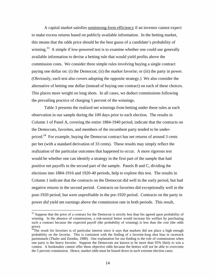
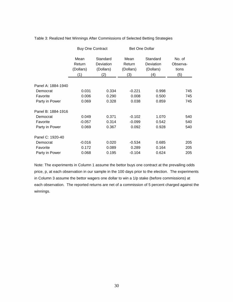
Table 3 presents the realized net winnings from betting under these rules at each

observation in our sample during the 100 days prior to each election. The results in

Column 1 of Panel A, covering the entire 1884-1940 period, indicate that the contracts on

the Democrats, favorites, and members of the incumbent party tended to be under-

priced.34 For example, buying the Democrat contract has net returns of around 3 cents

per bet (with a standard derivation of 33 cents). These results may simply reflect the

realization of the particular outcomes that happened to occur. A more rigorous test

would be whether one can identify a strategy in the first part of the sample that had

positive net payoffs in the second part of the sample. Panels B and C, dividing the

elections into 1884-1916 and 1920-40 periods, help to explore this test. The results in

Column 1 indicate that the contracts on the Democrat did well in the early period, but had

negative returns in the second period. Contracts on favorites did exceptionally well in the

post-1920 period, but were unprofitable in the pre-1920 period. Contracts on the party in

power did yield net earnings above the commission rate in both periods. This result,

33 Suppose that the price of a contract for the Democrat is strictly less than his agreed upon probability of winning. In the absence of commissions, a risk-neutral bettor would increase his welfare by purchasing such a contract because the expected payoff (the probability of winning) is less than the cost (the odds price). 34The result for favorites is of particular interest since it says that markets did not place a high enough probability on the favorite. This is consistent with the finding of a favorite-long shot bias in racetrack parimutuels (Thaler and Ziemba, 1988). One explanation for our finding is the role of commissions when one party is the heavy favorite. Suppose the Democrats are known to be more than 95% likely to win a contest. A bookmaker cannot offer these objective odds because the bettors will not be able to overcome the 5 percent commission. Hence, market odds must be biased down in such extreme election cases.

15

however, is not robust to changes in the wager structure. For example, as the figure in

Column 3 indicates, making a one-dollar wager on the party in power in the post-1920

period was an unprofitable strategy.35 These results as well as the more formal tests

reported in Rhode and Strumpf (2004) suggest that it was difficult to use public

information to construct a winning betting strategy. 36

A specific model of price dynamics allows us to statistically evaluate the

semistrong-form efficiency hypothesis. We presume that market participants have beliefs

about election outcomes, but face two forms of uncertainty. First, they know that each

day up until the election will bring some news shocks which we refer to as time-varying

uncertainty. Second, they have imperfect information about voter preferences, which we

refer to time-invariant uncertainty, and which is only revealed after the election. Then

semistrong-form efficiency, along with the model in the Appendix underlying equation

(1), requires that,

(2) VoteSharei* = (σ1

2(T-t)+σ22)0.5×priceit

* + νit

In this formula VoteShareit is the final vote share of the party specified in the contract in

national election i, priceit is the market price for the contract T-t days prior to the election,

and νit is a normally distributed and zero mean error term.37 The σ1 term represents the

time-varying uncertainty (presumed to be a priori identical across days), and it

diminishes in importance as the election date approaches (T-t decreases). σ2 is the time-

invariant uncertainty. The intuition is that current prices provide a forecast of the actual

election outcome, and when there is greater uncertainly, the price will be pushed toward

even odds because beliefs about the favorite are relatively weak.

Our empirical strategy provides a simple test of semistrong-form efficiency. We

will estimate equation (2) using the national election time series and treating the σ terms

as parameters to fit. Under the efficiency hypothesis, the estimated constant should be

35 Using the same one-dollar wager, Column 3 shows the Democrat and favorite strategies each lose money in at least one sub-period. 36 A useful contrast is the contemporary IEM WTA market. Using the available data for 1992, 1996, and 2000, buying a contract on the Democrats, the market favorite or the incumbent party are all at least as profitable as in the historical markets. This should be viewed with some caution due to the small number of elections in the IEM data. 37The star superscript is described in footnote 31, and it is still true that a related equation holds in a simple linear form without the star transform for closely contested elections.

16

zero. Intuitively, a constant represents the expected change in the vote share after

controlling for the market odds. So if the constant is positive, then the market is

consistently understating the election probability of the party listed on the contract, and

the semistrong-form efficiency hypothesis is rejected. Notice that by specifying the

contract is for Democrats, favorites, or candidates of the party in power, we can evaluate

violations of the sort highlighted with the betting strategies.

Table 4 displays non-linear least squares coefficients estimates of equation (2)

using the Democrat, market favorite, and party in power outcomes for the years 1884

through 1940. In each case, the constant term is statistically significantly different from

zero. Of greater economic significant is the implied pricing disparity. The bottom row

calculates the implied hypothetical price 21 days prior to Election Day in an even contest.

If the market were efficient, the implied price would exactly equal one half, the

probability of victory. Both the Democrat and party in power bets are significantly

under-priced and the favorite is slightly over-priced. It is also interesting that very

similar results are evident in the contemporary IEM WTA market. For example, using

data for Democrat’s from 1992, 1996 and 2000 we find a virtually identical constant as

that listed in the first column of Table 4.38

We also briefly discuss an analysis of semistrong-form efficiency for the

historical state-level bet markets. These markets are of interest since we can observe

multiple prices at one time, and so do not have to be as concerned about time series

issues. At the same time, these markets are much thinner than those for the national

contest. We find that two of the three strategies discussed earlier are profitable: betting

on the Democratic candidate yields an average daily return of $0.06 and betting on the

candidate which the market favors in the state yields $0.14 (these values are for daily

purchases of single share and include commissions). We can also consider regression

evidence on market efficiency using the cross-sectional analogue of equation (2) which is

derived in the Appendix,

(3) VoteSharei* = σ×pricei

* + εi

38 The estimated uncertainty terms, σ1

2 and σ22, are each an order of magnitude smaller in the contemporary

IEM. This likely reflects the wider distribution of public information about the candidates and the presence of scientific polls.

17

This formula states that the actual vote share in state i, VoteSharei, differs from the

current market beliefs, pricei, chiefly by some shock term, εi. The shock again represents

any future uncertainty, and σ is the average standard deviation across states of these

terms. The equation captures the efficiency hypothesis since it says that deviations from

the current market price cannot be predicted. This means that the estimated constant and

all publicly observed covariates should have zero parameters. Table 5 presents the

coefficients using Democratic contracts for the years with available data (1896, 1912,

1932, and 1944). The first column shows that the estimated constant is not statistically

different from zero. However, the second column shows that several covariates help

explain vote outcomes even after controlling for market prices. In particular, the lagged

vote share has a significant and positive effect. Even after controlling for the market

prices, a one percent increase in previous vote share implies a half a percent increase in

current vote share. The final column shows that polling data (which is available in the

last two elections) not only has a large positive effect, but it subsumes the explanatory

ability of market prices. In total these results suggest a marked departure from

semistrong-form efficiency in the state-level betting markets. This result is perhaps

unsurprising given that this market was a minor footnote relative to the far more popular

market on the overall national winner.

Finally we consider strong-form efficiency, whether an investor can earn excess

profits using private information. While it is difficult to quantify this hypothesis, there

are several reports of insiders profiting from superior information about specific states.

As examples, in 1916, some West Coast investors wagered heavily on Wilson because

they believed he would unexpectedly win California, which he did (Wall Street Journal,

31 Oct. 1916, p. 8). Leveraging on superior local information, several Ohioans fronted

by Tex Rickard placed a $60,000 wager on Wilson to win their state (New York Times, 28

Oct. 1916, p. 1). These must have been strong beliefs since the wager moved the odds

price by nearly ten percentage points, and again the investors proved to be correct. It

seems that insiders were able to profit from their information advantage, but note

rejections of strong efficiency are typical of most capital markets.

In conclusion, the historical betting markets do not meet all of the exacting

conditions for efficiency, but the deviations were not usually large enough to generate

18

consistently profitable betting strategies for the national outcome using public

information.39 The performance of the market was comparable to its modern

counterparts and, given the barriers to efficiency discussed earlier, quite remarkable.

VII: The Decline of Political Wagering

The newspapers reported substantially less betting activity in specific contests

(1880, 1908, 1912) and especially after 1940. In part, this reflects the reluctance of

newspapers to give publicity to activities that many concerned unethical. There were

frequent complaints that election betting was immoral and contrary to republican values.

Among the issues critics raised were moral hazard, election tampering, information

withholding, and strategic manipulation.40

In response to such concerns, New York state laws did increasingly attempt to

limit organized election betting. Casual bets between private individuals always

remained legal in New York. Betting on elections nominally disqualified the participants

from voting and the legal system also discouraged using the courts to enforce gambling

contracts. Following the troubles associated with John Morrissey’s cancellation of the

1876 election pools, the legislature passed laws against pool-selling, which were enforced

rigorously through the 1880 election. But as often happened, enforcement efforts weaken

and the sporting interests found loopholes around the existing laws. For the next quarter

century, election betting flourished. At the behest of New York governor, Charles

Hughes, the state outlawed in 1908 and 1910, respectively, professional bookmaking

employing written bets and oral bets. The prohibition was directed primarily towards

horse racing, but had the effect of suppressing open election betting in 1908 and 1912.41

39The wager markets on state election outcomes more convincingly fails the efficiency conditions. This result is unsurprising given that the state markets were far thinner than the national market. 40 For selected historical criticisms of election betting, see New York Tribune, 18 Nov. 1888, p. 6; New York Times, 28 Oct. 1896, p. 1; 3 Nov. 1896, p. 2; Washington Post, 28 Oct. 1912, p. 2. For a recent discussion, see Hanson (2003). 41 The Curb brokers initially responded to the 1908 laws by revising the contract form – creating a memorandum between “friends” to transfer money conditional on the election outcome—and by raising the commission to reflect the increased trouble and legal exposure. New York Tribune, 30 Oct. 1908, p. 1. See also New York Times, 22 Oct. 1909, p. 1; 11 July 1912, p. 10; 18 July 1912, p. 1.

19

Ironically, by the final month of the 1916 contest between Hughes and President Wilson,

election betting in the financial district was back in full swing. Although there were

subsequent waves of anti-gambling policing, it is possible that New York’s legalization

of pari-mutuel betting on horse races in 1939 actually did more to reduce book-making

on elections. Individuals interested in gambling now has several contests per day to

wager on that promised immediate rewards rather than a single political contest stretching

over several months. Along with the rising importance of illegal betting on sports such as

baseball, this shifted the focus of the bookmakers, the suppliers.

New York State was not alone in changing the legal environment for election

betting. The Stock Exchanges also periodically enacted regulations to limit involvement

of their members. The Exchanges characteristically did not like the public to associate

their socially productive risk-sharing and risk-taking functions with gambling on sporting

events. The World Series, horse races, and prizefights were viewed as zero-sum

entertainment activities whose outcomes did not affect the broader world. Arguably

betting on elections belonged in the risk insurance category and the information that the

betting market provided had “real-world” value, unlike knowing the winner of the sports

tournament. One could readily imagine a risk-averse owner of an investor project betting

for a candidate unfavorable to the project to hedge against a “bad” election outcome. But

often it appears the bets were partisan or sentimental in the sense that bettors took the

side of their preferred candidate. The major exceptions occurred after odds have changed

when partisans would hedge existing bets by taking the other side.

Fear of association with gambling and bucket shop operations led the Exchanges

to distance themselves from election betting. For example, before the 1912 party

conventions, the New York Curb Association reminded its members that placing or

accepting bets was contrary to New York laws. “Any member found betting, placing

bets, or reporting alleged bets to the press will be charged with action detrimental to the

interest of the association, which may lead to his suspension.”42 In May 1924, both the

New York Stock Exchange and the Curb Market passed resolutions barring their

members from engaging election gambling. Again in late 1927, both exchanges blocked

42 Wall Street Journal, 8 June 1912, p. 5.

20

the use of “when issued” contracts to discourage gambling.43 There are also suggestions

in the business press that in the mid-1930s, as the New Deal securities regulations were

taking effect, the Wall Street brokerages shied away from election betting for fear of

appearing too partisan, or rather anti-Roosevelt.

Another force working to diminish election betting in the 1930s was that publicly

traded securities, particularly those of electrical utilities, were becoming closer substitutes

for wagers on Roosevelt in 1936 and 1940.44 Large players could speculate on the

election outcome through the Stock Exchange by going long or short on utility stock

without risking running afoul of the law or having the betting commissioner abscond with

the stakes. In addition, it was possible to settle up before the election occurred.

A final force pushing election betting underground, or at least out of the

newspapers was the rise of scientific polling. As noted above, one of the functions of

reporting Wall Street betting odds was to provide the best available aggregate

information. Following the success of Gallup and other scientific pollsters in the 1936

election, many newspapers stopped lending credence to the Literary Digest poll. The

scientific polls, available on a weekly basis, provided the media with a ready substitute

for the betting odds, one less subject to the moral objections against gambling. Our

survey of the Washington Post and New York Times indicates that articles on the Literary

Digest poll began to out-number those on election betting in 1924 and 1928, respectively.

Those related to the Gallup poll began to appear in 1936 and to out-number those in the

other two categories by 1940. What election betting that continued to occur received far

less media attention.45

43 Wall Street Journal, 23 Dec. 1927, p. 11. Reports indicate that low profitability of stake holding in the 1924 election rather than the tightening regulatory regimes was responsible for the decline in Wall Street election betting. New York Times, 27 Sept. 1928, p. 23. Note that the high volume of stock transaction in the late 1920s—when the New York Stock Exchange frequently closed on Saturdays to handle backed-up orders—may have also drawn brokers away from election betting. A high volume of stock trading in 1916, it was said, delayed the takeoff in betting until the last month of the campaign. New York Times, 24 Sept. 1916, p. E5. 44 New York Herald Tribune, 2 Nov. 1940, p. 23; Wall Street Journal, 8 June 1936, p. 15; 13 Nov. 1944, p. 13. 45 Justin Wolfers has raised the insightful observation that the appearance of scientific polls created a new set of insiders – those with access to the results before publication – that may have made outsiders less willing to participate in the betting markets. These emerging information asymmetries may have contributed to the market’s collapse.

21

VIII: Lessons for the Future

Wagering on presidential elections has a long tradition in the U.S., with large and

often well-organized markets operating for over three-quarters of a century before the

Second World War. The resulting betting odds proved remarkably prescient and almost

always correctly predicted election outcomes well in advance, despite the absence of

scientific polls.

This historical experience suggests a promising role for other prediction markets.

While a substantial body of experimental research has hinted that asset markets can

successfully aggregate information (Forsythe, et al., 1982 and Plott and Sunder, 1988),

recent experience indicates public skepticism about applying markets to novel

situations.46 This was most clearly evident in the Policy Analysis Market (proposed in

2003) which sought to provide a market consensus about international political

developments. Critics argued that this market was subject to manipulation by insiders

and might allow extremists to profit financially from their actions. But these concerns

were also evident in the historical wagering on presidential elections, with partisans

serving as active participants and contemporary fears of election tampering. Although

vast sums of money were at stake, we are not aware of any evidence that the political

process was seriously corrupted by the presence of a wagering market. This analysis

suggests many current concerns about the appropriateness of prediction markets are not

well founded in the historical record. Simply put, election betting flourished for decades

before the Second World War yet the Republic did not fall or even falter as a

consequence.. We hope this historical experience with actual markets, rather than solely

polemics, will inform future discussions of possible applications of prediction markets.

The analysis of political betting markets also encourages us to rethink questions

about why people participate in politics. Rational choice models of politics have severe

difficulties explaining why people vote given voting is costly and the probability of being

pivotal is negligibly small. The experience of the political betting markets suggests a

46 The informational efficiency of prediction markets has also been investigated in the field, such as the difficulty of manipulating horse track parimutuels (Camerer, 1998). For one of the few evaluations of non-sports prediction markets, see Leigh, et al. (2003).

22

parallel between being a political participant and being a sports fan. Hoping that the right

sort (typically one’s own sort) rule the government and rooting for the right team

(typically the home team) are both matters of identity. Our review of the newspaper

evidence indicates the participants in the political betting markets typically sought to

intensify their stakes in the election, in effect to double-down by backing their opinions

and preferences with money. Betting to insure against loss was rarely mentioned. The

same appears true of sports betting (Strumpf, 2003). For many, expressing feelings of

affiliation is apparently worth the price.

23

References Berg, Joyce, Forrest Nelson and Thomas Rietz (2003). “Accuracy and Forecast Standard Error of Prediction Markets.” University of Iowa working paper. Camerer, Colin (1998) “Can Asset Markets be Manipulated? A Field Experiment with Racetrack Betting.” Journal of Political Economy. 106:457-82. Fama, Eugene (1970). “Efficient Capital Markets: A Review of Theory and Empirical Work.” Journal of Finance. 25: 383-417. Forsythe, Robert, Thomas Palfrey, and Charles Plott (1982). “Asset Valuation in an Experimental Market.” Econometrica. 50: 537-568. Gilliams, E. Leslie (1901). “Election Bets in America.” Strand Magazine. XXI: 185-191. Hanson, Robin (2003). “Shall We Vote Values, But Bet of Beliefs?” (Sept.) George Mason Working Paper. Leigh, Andrew, Justin Wolfers and Eric Zitzewitz (2003). “What Do Financial Markets Think of War in Iraq?” NBER working paper 9587. Morris, Edmund (2001). The Rise of Theodore Roosevelt. (rev. ed.) New York: Modern Library. Plott, Charles, and Shyam Sunder (1988). “Rational Expectations and the Aggregation of Diverse Information in Laboratory Security Markets.” Econometrica. 56: 1085-1118. Pietrusza, David (2003). Rothstein: The Life, Times, and Murder of the Criminal Genius Whi Fixed the 1919 World Series. (New York: Carroll & Graf).

Roll, Richard (1984). “Orange Juice and Weather.” American Economic Review. 74: 861-880. Samuelson, Paul (1965). “Proof that Properly Anticipated Prices Fluctuate Randomly.” Industrial Management Review. 41-49. Strumpf, Koleman (2003). “Illegal Sports Bookmakers.” UNC working paper. Thaler, Richard and William Ziemba (1988). “Parimutuel Betting Markets: Racetracks and Lotteries.” Journal of Economic Perspectives. Spring (2:2), 161-174. Newspapers: Chicago Tribune, New York Sun, New York Times, New York Tribune, New York World, St. Louis Post-Dispatch, Wall Street Journal, Washington Post.

24

Appendix: Efficiency in the Presidential Betting Market

National Elections Markets (time series): Weak form and Semistrong-form

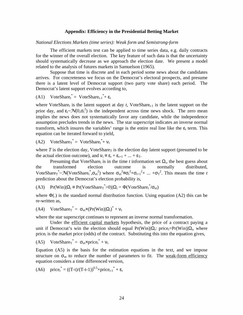
The efficient markets test can be applied to time series data, e.g. daily contracts for the winner of the overall election. The key feature of such data is that the uncertainty should systematically decrease as we approach the election date. We present a model related to the analysis of futures markets in Samuelson (1965).

Suppose that time is discrete and in each period some news about the candidates arrives. For concreteness we focus on the Democrat’s electoral prospects, and presume there is a latent level of Democrat support (two party vote share) each period. The Democrat’s latent support evolves according to,

(A1) VoteSharet* = VoteSharet-1

*+ εt

where VoteSharet is the latent support at day t, VoteSharet-1 is the latent support on the prior day, and εt~N(0,σt

2) is the independent across time news shock. The zero mean implies the news does not systematically favor any candidate, while the independence assumption precludes trends in the news. The star superscript indicates an inverse normal transform, which insures the variables’ range is the entire real line like the εt term. This equation can be iterated forward to yield,

(A2) VoteShareT* = VoteSharet

*+ νt

where T is the election day, VoteShareT is the election day latent support (presumed to be the actual election outcome), and νt ≡ εt + εt+1 + ... + εT.

Presuming that VoteSharet is in the time t information set Ωt, the best guess about the transformed election outcome is normally distributed, VoteShareT

*~N(VoteSharet*,σνt

2) where σνt2≡σt

2+σt+12+ ... +σT

2. This means the time t prediction about the Democrat’s election probability is,

(A3) Pr(Win)|Ωt ≡ Pr(VoteShareT*>0)|Ωt = Φ(VoteSharet

*/σνt)

where Φ(.) is the standard normal distribution function. Using equation (A2) this can be re-written as,

(A4) VoteShareT* = σνt×(Pr(Win)|Ωt)

* + νt

where the star superscript continues to represent an inverse normal transformation. Under the efficient capital markets hypothesis, the price of a contract paying a

unit if Democrat’s win the election should equal Pr(Win)|Ωt: pricet=Pr(Win)|Ωt, where pricet is the market price (odds) of the contract. Substituting this into the equation gives,

(A5) VoteShareT* = σνt×pricet

* + νt

Equation (A5) is the basis for the estimation equations in the text, and we impose structure on σνt to reduce the number of parameters to fit. The weak-form efficiency equation considers a time differenced version,

(A6) pricet* = ((T-t)/(T-t-1))0.5×pricet-1

* + εt

25

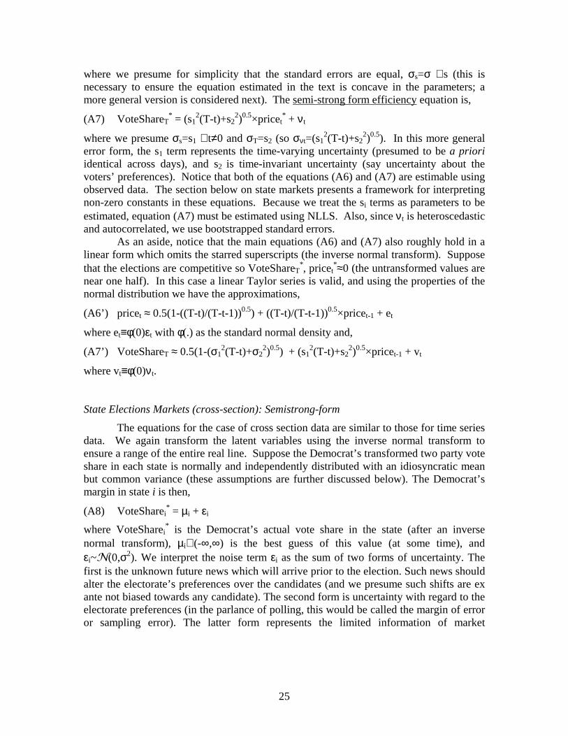
where we presume for simplicity that the standard errors are equal, σs=σ ∀ s (this is necessary to ensure the equation estimated in the text is concave in the parameters; a more general version is considered next). The semi-strong form efficiency equation is,

(A7) VoteShareT* = (s1

2(T-t)+s22)0.5×pricet

* + νt

where we presume σs=s1 ∀ t≠0 and σT=s2 (so σνt=(s12(T-t)+s2

2)0.5). In this more general error form, the s1 term represents the time-varying uncertainty (presumed to be a priori identical across days), and s2 is time-invariant uncertainty (say uncertainty about the voters’ preferences). Notice that both of the equations (A6) and (A7) are estimable using observed data. The section below on state markets presents a framework for interpreting non-zero constants in these equations. Because we treat the si terms as parameters to be estimated, equation (A7) must be estimated using NLLS. Also, since νt is heteroscedastic and autocorrelated, we use bootstrapped standard errors.

As an aside, notice that the main equations (A6) and (A7) also roughly hold in a linear form which omits the starred superscripts (the inverse normal transform). Suppose that the elections are competitive so VoteShareT

*, pricet*≈0 (the untransformed values are

near one half). In this case a linear Taylor series is valid, and using the properties of the normal distribution we have the approximations,

(A6’) pricet ≈ 0.5(1-((T-t)/(T-t-1))0.5) + ((T-t)/(T-t-1))0.5×pricet-1 + et

where et≡φ(0)εt with φ(.) as the standard normal density and,

(A7’) VoteShareT ≈ 0.5(1-(σ12(T-t)+σ2

2)0.5) + (s12(T-t)+s2

2)0.5×pricet-1 + vt

where vt≡φ(0)νt.

State Elections Markets (cross-section): Semistrong-form

The equations for the case of cross section data are similar to those for time series data. We again transform the latent variables using the inverse normal transform to ensure a range of the entire real line. Suppose the Democrat’s transformed two party vote share in each state is normally and independently distributed with an idiosyncratic mean but common variance (these assumptions are further discussed below). The Democrat’s margin in state i is then,

(A8) VoteSharei* = µi + εi

where VoteSharei* is the Democrat’s actual vote share in the state (after an inverse

normal transform), µi∈ (-∞,∞) is the best guess of this value (at some time), and εi~N(0,σ2). We interpret the noise term εi as the sum of two forms of uncertainty. The first is the unknown future news which will arrive prior to the election. Such news should alter the electorate’s preferences over the candidates (and we presume such shifts are ex ante not biased towards any candidate). The second form is uncertainty with regard to the electorate preferences (in the parlance of polling, this would be called the margin of error or sampling error). The latter form represents the limited information of market

26

participants. The standard deviation σ represents the importance of both form forms of uncertainty.47

We presume the market participants know the structural parameters µi and σ, but the econometrician does not. The Democrat’s probability of winning the state, given the current information set Ω, is,

(A9) Pr(Win i)|Ω ≡ Pr(VoteSharei*>0) = Φ(µi/σ)

Using equation (A8) this can be re-written as,

(A10) VoteSharei* = σ(Pr(Win i)|Ω)* + εi

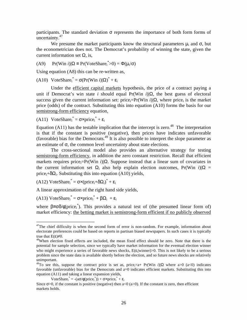
Under the efficient capital markets hypothesis, the price of a contract paying a unit if Democrat’s win state i should equal Pr(Win i)|Ω, the best guess of electoral success given the current information set: pricei=Pr(Win i)|Ω, where pricei is the market price (odds) of the contract. Substituting this into equation (A10) forms the basis for our semistrong-form efficiency equation,

(A11) VoteSharei* = σ×pricei

* + εi

Equation (A11) has the testable implication that the intercept is zero.48 The interpretation is that if the constant is positive (negative), then prices have indicates unfavorable (favorable) bias for the Democrats.49 It is also possible to interpret the slope parameter as an estimate of σ, the common level uncertainty about state elections. The cross-sectional model also provides an alternative strategy for testing semistrong-form efficiency, in addition the zero constant restriction. Recall that efficient markets requires pricei=Pr(Win i)|Ω. Suppose instead that a linear sum of covariates in the current information set Ωi also help explain election outcomes, Pr(Win i)|Ω = pricei+δΩi. Substituting this into equation (A10) yields,

(A12) VoteSharei* = σ×(pricei+δΩi)

* + εi

A linear approximation of the right hand side yields,

(A13) VoteSharei* = σ×pricei

* + βΩi + εi

where β≡σδ/φ(pricei*). This provides a natural test of (the presumed linear form of)

market efficiency: the betting market is semistrong-form efficient if no publicly observed

47The chief difficulty is when the second form of error is non-random. For example, information about electorate preferences could be based on reports in partisan biased newspapers. In such cases it is typically true that E(ε)≠0. 48When election fixed effects are included, the mean fixed effect should be zero. Note that there is the potential for sample selection, since we typically have market information for the eventual election winner who might experience a series of favorable news shocks, E(εi|winner)>0. This is not likely to be a serious problem since the state data is available shortly before the election, and so future news shocks are relatively unimportant. 49To see this, suppose the contract price is set as, pricei=a+ Pr(Win i)|Ω where a>0 (a<0) indicates favorable (unfavorable) bias for the Democrats and a=0 indicates efficient markets. Substituting this into equation (A11) and taking a linear expansion yields,

VoteSharei* = -(aσ/φ(pricei

*)) + σ×pricei* + εi

Since σ>0, if the constant is positive (negative) then a<0 (a>0). If the constant is zero, then efficient markets holds.

27

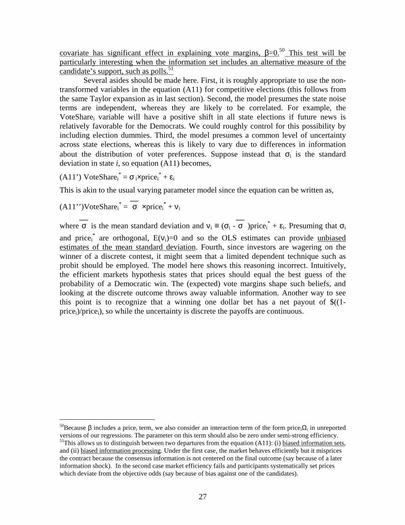
covariate has significant effect in explaining vote margins, β=0.50 This test will be particularly interesting when the information set includes an alternative measure of the candidate’s support, such as polls.51

Several asides should be made here. First, it is roughly appropriate to use the non-transformed variables in the equation (A11) for competitive elections (this follows from the same Taylor expansion as in last section). Second, the model presumes the state noise terms are independent, whereas they are likely to be correlated. For example, the VoteSharei variable will have a positive shift in all state elections if future news is relatively favorable for the Democrats. We could roughly control for this possibility by including election dummies. Third, the model presumes a common level of uncertainty across state elections, whereas this is likely to vary due to differences in information about the distribution of voter preferences. Suppose instead that σi is the standard deviation in state i, so equation (A11) becomes,

(A11’) VoteSharei* = σ i×pricei

* + εi

This is akin to the usual varying parameter model since the equation can be written as,

(A11’’)VoteSharei* = σ ×pricei

* + νi

where σ is the mean standard deviation and νi ≡ (σi - σ )pricei* + εi. Presuming that σi

and pricei* are orthogonal, E(νi)=0 and so the OLS estimates can provide unbiased

estimates of the mean standard deviation. Fourth, since investors are wagering on the winner of a discrete contest, it might seem that a limited dependent technique such as probit should be employed. The model here shows this reasoning incorrect. Intuitively, the efficient markets hypothesis states that prices should equal the best guess of the probability of a Democratic win. The (expected) vote margins shape such beliefs, and looking at the discrete outcome throws away valuable information. Another way to see this point is to recognize that a winning one dollar bet has a net payout of $((1-pricei)/pricei), so while the uncertainty is discrete the payoffs are continuous.

50Because β includes a pricei term, we also consider an interaction term of the form priceiΩi in unreported versions of our regressions. The parameter on this term should also be zero under semi-strong efficiency. 51This allows us to distinguish between two departures from the equation (A11): (i) biased information sets, and (ii) biased information processing. Under the first case, the market behaves efficiently but it misprices the contract because the consensus information is not centered on the final outcome (say because of a later information shock). In the second case market efficiency fails and participants systematically set prices which deviate from the objective odds (say because of bias against one of the candidates).

28

Table 1: New York Election Betting Volume

New York Betting Volume

2002 dollars Dollars per Dollars per

(millions) Votes Cast Campaign Spending

1884 13.7 1.36 0.278

1888 37.6 3.30 0.907

1892 14.8 1.23 0.185

1896 10.7 0.77 0.124

1900 63.9 4.57 0.876

1904 50.3 3.72 0.894

1908 7.7 0.52 0.174

1912 4.6 0.30 0.087

1916 165.0 8.90 2.116

1920 44.9 1.68 0.726

1924 21.0 0.72 0.373

1928 10.5 0.29 0.086

Average 37.0 2.28 0.532

Sources: New York World: 9 Nov. 1888, pp. 1-2; 4 Nov. 1896, p. 11; 8 Nov. 1900, p. 4; 3

Nov. 1920, p. 4; New York Tribune: 8 Nov 1900, p. 6; 9 Nov. 1900, p. 3; Wall Street

Journal: 3 Nov. 1908, p. 7; 6 Nov. 1924, p. 10; New York Times: 8 Nov. 1900, p. 5; 8

Nov. 1904, p. 1; 10 Nov. 1904, p. 5; 7 Nov. 1912, p.1; 11 Nov. 1916, p. 12; 31 Aug.

1924, p.3; 6 Nov. 1928, p. 15. Other sources (New York Tribune 6 Nov. 1928, p.3)

suggest the 1928 figures are too low and that although exact numbers are not available,

betting in the 1930s were more active (New York Times, 19 Oct. 1932, p. 17; 24 Sept.

1936, p. 2). On 4 Dec. 1928, p. 1, the Washington Post noted that legendary gambler

Arnold Rothstein won $500,000 on $1.7 million in wagers on the 1928 election, but his

murder cancelled the bets.

The number of votes cast and the total campaign spending of the national presidential

campaigns are from Historical Statistics Y135, pp. 1078-79 and Series Y187-88, p. 1081,

respectively.

29

Table 2: Date of Crossing Odds Price Thresholds in Selected Elections

Year Candidate Absolute Popular Days Before Election for Odds Prices:

Vote Margin 0.66 0.75 0.80

1920 Harding 26.2% 125days 49 43

1924 Coolidge 25.2 120 113 18

1936 F. Roosevelt 24.3 3 3 --

1904 T. Roosevelt 18.8 49 24 18

1932 F. Roosevelt 17.7 36 8 4

1928 Hoover 17.3 138 46 13

1912 Wilson 14.4 111 63 12

1900 McKinley 6.2 133 33 21

1908 Taft 8.4 115 115 6

1896 McKinley 4.4 97 20 1

Source: Vote Margins from Historical Statistics, Y 79-83, pp. 1073-74.

30

Table 3: Realized Net Winnings After Commissions of Selected Betting Strategies Buy One Contract Bet One Dollar Mean Standard Mean Standard No. of Return Deviation Return Deviation Observa- (Dollars) (Dollars) (Dollars) (Dollars) tions (1) (2) (3) (4) (5)

Panel A: 1884-1940 Democrat 0.031 0.334 -0.221 0.998 745 Favorite 0.006 0.290 0.008 0.500 745 Party in Power 0.069 0.328 0.038 0.859 745 Panel B: 1884-1916 Democrat 0.049 0.371 -0.102 1.070 540 Favorite -0.057 0.314 -0.099 0.542 540 Party in Power 0.069 0.367 0.092 0.928 540 Panel C: 1920-40 Democrat -0.016 0.020 -0.534 0.685 205 Favorite 0.172 0.089 0.289 0.164 205 Party in Power 0.068 0.195 -0.104 0.624 205

Note: The experiments in Column 1 assume the bettor buys one contract at the prevailing odds

price, p, at each observation in our sample in the 100 days prior to the election. The experiments

in Column 3 assume the bettor wagers one dollar to win a 1/p stake (before commissions) at

each observation. The reported returns are net of a commission of 5 percent charged against the

winnings.

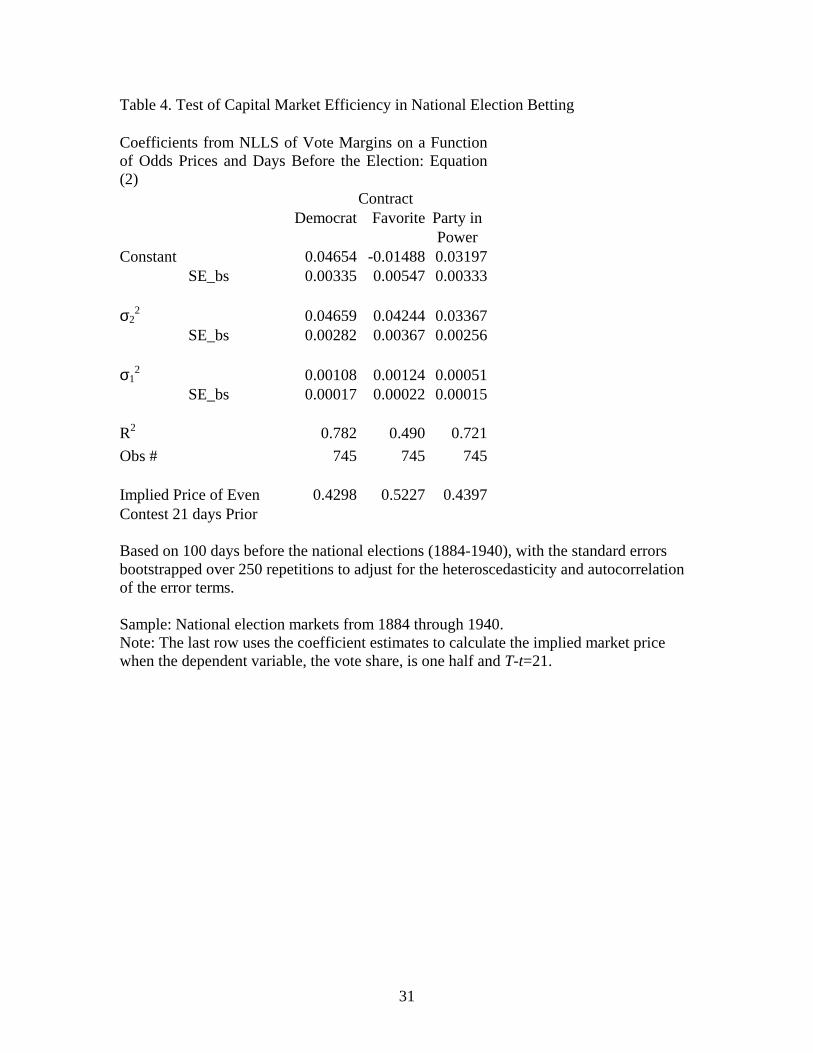
31

Table 4. Test of Capital Market Efficiency in National Election Betting Coefficients from NLLS of Vote Margins on a Function of Odds Prices and Days Before the Election: Equation (2) Contract Democrat Favorite Party in Power Constant 0.04654 -0.01488 0.03197

SE_bs 0.00335 0.00547 0.00333 σ2

2 0.04659 0.04244 0.03367 SE_bs 0.00282 0.00367 0.00256

σ1

2 0.00108 0.00124 0.00051 SE_bs 0.00017 0.00022 0.00015

R2 0.782 0.490 0.721

Obs # 745 745 745 Implied Price of Even 0.4298 0.5227 0.4397 Contest 21 days Prior Based on 100 days before the national elections (1884-1940), with the standard errors bootstrapped over 250 repetitions to adjust for the heteroscedasticity and autocorrelation of the error terms. Sample: National election markets from 1884 through 1940. Note: The last row uses the coefficient estimates to calculate the implied market price when the dependent variable, the vote share, is one half and T-t=21.

32

Table 5: Test of Capital Market Efficiency in State Election Betting Coefficients from OLS regression of Actual State Democratic Vote Shares on a Function of Odds Prices and Publicly Observed Covariates: Equation (3) Covariate (i) (ii) (iii) (iv) Constant 0.036

(0.035) 0.129 (0.140)

0.093 (0.026)

0.199 (0 .017)

Pricei* 0.491

(0.057) 0.259 (0.100)

0.505 (0.055)

-0.037 (0.016)

Lagged VoteSharei* 0.559

(0.140) 0.421

(0.113) Democrat Incumbent -0.218

(0.149) -0.223

(0.036) Distance from NYCi 0.093

(0.054) 0.022

(0.011) Polli

* 0.781 (0.038)

N 188 186 96 96 R2 0.51 0.71 0.56 0.94 Robust standard errors (with year clusters) are reported beneath the parameter estimates. i subscripts indicate state-specific variable and the star superscript indicates an inverse normal transformation. The additional covariates are the Democratic vote share in the state during the prior election (Lagged VoteSharei), an indicator for a Democratic incumbent (Democrat Incumbent), distance of the state capital from New York city, in thousands of miles (Distance from NYC), and the Democrat’s poll totals in the state (Polli). The distance variable is included since it might reflect information lags for more distant states The estimates are for elections with state data, and the sample includes the 48 states in 1896, 1912, 1932, 1944 (the estimates in columns (iii) and (iv) only include 1932 and 1944). The market price on Democrat’s, pricei, are mostly from the end of October or early November. The polling data, Polli, is from the Literary Digest in 1932 and from Gallup in 1944 (polling data is unavailable in earlier years).

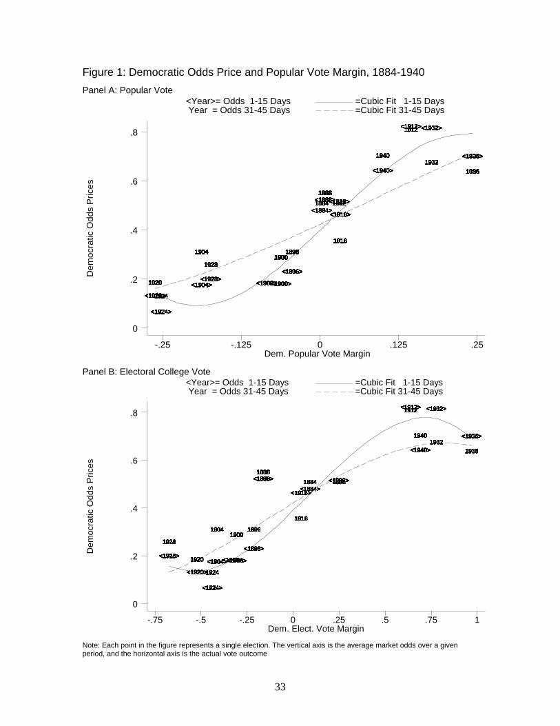
33

Figure 1: Democratic Odds Price and Popular Vote Margin, 1884-1940

Panel A: Popular Vote D

emoc

ratic

Odd

s P

rices

Dem. Popular Vote Margin

<Year>= Odds 1-15 Days =Cubic Fit 1-15 Days Year = Odds 31-45 Days =Cubic Fit 31-45 Days

-.25 -.125 0 .125 .25

0

.2

.4

.6

.8

<1920><1920><1920><1920><1920><1920><1920><1920><1920><1920><1920><1920><1920><1920><1920><1920><1920><1920><1920><1920><1920><1920><1920><1920><1920><1920><1920><1920><1920><1920><1920><1920><1920><1920><1920><1920><1920><1920><1920><1920><1920><1920><1920><1920><1920><1920><1920><1920><1920><1920>

<1924><1924><1924><1924><1924><1924><1924><1924><1924><1924><1924><1924><1924><1924><1924><1924><1924><1924><1924><1924><1924><1924><1924><1924><1924><1924><1924><1924><1924><1924><1924><1924><1924><1924><1924><1924><1924><1924><1924><1924><1924><1924><1924><1924><1924><1924><1924><1924><1924><1924><1924><1924><1924><1924><1924><1924><1924><1924><1924><1924><1924><1924><1924><1924><1924><1924><1924><1924><1924><1924><1924><1924><1924><1924><1924><1924><1924><1924><1924><1924><1924><1924><1924><1924><1924><1924><1924><1924><1924><1924><1924><1924>

<1904><1904><1904><1904><1904><1904><1904><1904><1904><1904><1904><1904><1904><1904><1904><1904><1904><1904><1904><1904><1904><1904><1904><1904><1904><1904><1904><1904><1904><1904><1904><1904><1904><1904><1904><1904><1904><1904><1904><1904><1904><1904><1904><1904><1904><1904><1904><1904><1904><1904><1904><1904><1904><1904><1904><1904><1904><1904><1904><1904><1904><1904><1904><1904><1904><1904><1904><1904><1904><1904><1904><1904><1904><1904><1904><1904><1904><1904><1904><1904><1904><1904><1904><1904><1904><1904><1904><1904><1904><1904><1904><1904><1904><1904><1904><1904><1904><1904><1904><1928><1928><1928><1928><1928><1928><1928><1928><1928><1928><1928><1928><1928><1928><1928><1928><1928><1928><1928><1928><1928><1928><1928><1928><1928><1928><1928><1928><1928><1928><1928><1928><1928><1928><1928><1928><1928><1928><1928><1928><1928><1928><1928>

<1908><1908><1908><1908><1908><1908><1908><1908><1908><1908><1908><1908><1908><1908><1908><1908><1908><1908><1908><1908><1908><1908><1908><1908><1908><1908><1908><1908><1908><1908><1908><1908><1908><1908><1908><1908><1908><1908><1908><1908><1908><1908><1908><1900><1900><1900><1900><1900><1900><1900><1900><1900><1900><1900><1900><1900><1900><1900><1900><1900><1900><1900><1900><1900><1900><1900><1900><1900><1900><1900><1900><1900><1900><1900><1900><1900><1900><1900><1900><1900><1900><1900><1900><1900><1900><1900><1900><1900><1900><1900><1900><1900><1900><1900><1900><1900><1900><1900><1900><1900><1900><1900><1900><1900><1900><1900><1900><1900><1900><1900><1900><1900><1900><1900><1900><1900><1900><1900><1900><1900><1900><1900><1900><1900><1900>

<1896><1896><1896><1896><1896><1896><1896><1896><1896><1896><1896><1896><1896><1896><1896><1896><1896><1896><1896><1896><1896><1896><1896><1896><1896><1896><1896><1896><1896><1896><1896><1896><1896><1896><1896><1896><1896><1896><1896><1896><1896><1896><1896><1896><1896><1896><1896><1896><1896><1896><1896><1896><1896><1896><1896><1896>

<1884><1884><1884><1884><1884><1884><1884><1884><1884><1884><1884><1884><1884><1884>

<1888><1888><1888><1888><1888><1888><1888><1888><1888><1888><1888><1888><1888><1888><1888><1888><1888><1888><1888><1888><1888><1888><1888><1888><1888><1888><1888><1888><1888><1888><1888><1888><1888><1888><1888><1888><1888><1888><1888><1888><1892><1892><1892><1892><1892><1892><1892><1892><1892><1892><1892><1892><1892><1892><1892><1892><1892><1892><1892><1892><1892><1892><1892><1892><1892><1892><1892><1892><1892><1892><1892><1892><1892><1892><1892><1892><1892><1892><1892><1892><1892><1892><1892><1892><1892><1892><1892><1892>

<1916><1916><1916><1916><1916><1916><1916><1916><1916><1916><1916><1916><1916><1916><1916><1916><1916><1916><1916><1916><1916><1916><1916><1916><1916><1916><1916><1916><1916><1916><1916><1916><1916><1916><1916><1916><1916><1916><1916><1916><1916><1916><1916><1916><1916><1916><1916><1916><1916><1916><1916><1916><1916><1916><1916><1916><1916><1916><1916><1916><1916><1916><1916><1916><1916><1916><1916><1916><1916><1916><1916><1916><1916><1916><1916><1916><1916><1916><1916><1916><1916><1916><1916><1916><1916><1916><1916><1916><1916><1916><1916><1916><1916><1916><1916><1916><1916><1916><1916><1916><1916><1916><1916><1916><1916><1916><1916><1916><1916><1916><1916><1916><1916><1916><1916><1916><1916><1916><1916><1916><1916><1916><1916><1916><1916><1916><1916><1916><1916><1916><1916><1916><1916><1916><1916><1916><1916><1916><1916><1916><1916><1916><1916><1916><1916><1916><1916><1916><1916><1916><1916><1916><1916><1916>

<1940><1940><1940><1940><1940><1940><1940><1940><1940><1940><1940><1940><1940><1940><1940><1940><1940><1940><1940><1940><1940>

<1912><1912><1912><1912><1912><1912><1912><1912><1912><1912><1912><1912><1912><1912><1912><1912><1912><1912><1912><1912><1912><1912><1912><1912><1912><1912><1912><1912><1912><1912><1912><1912><1912><1912><1912><1912><1912><1912><1912><1912><1912><1912><1912><1912><1932><1932><1932><1932><1932><1932><1932><1932><1932><1932><1932><1932><1932><1932><1932><1932><1932><1932><1932><1932><1932><1932><1932><1932>

<1936><1936><1936><1936><1936><1936><1936><1936><1936><1936><1936><1936><1936><1936><1936><1936><1936><1936><1936><1936><1936><1936><1936><1936><1936><1936><1936><1936><1936><1936><1936><1936><1936><1936><1936><1936><1936><1936><1936><1936><1936><1936><1936><1936><1936>

19201920192019201920192019201920192019201920192019201920192019201920192019201920192019201920192019201920192019201920192019201920192019201920192019201920192019201920192019201920192019201920192019201920

19241924192419241924192419241924192419241924192419241924192419241924192419241924192419241924192419241924192419241924192419241924192419241924192419241924192419241924192419241924192419241924192419241924192419241924192419241924192419241924192419241924192419241924192419241924192419241924192419241924192419241924192419241924192419241924192419241924192419241924192419241924

190419041904190419041904190419041904190419041904190419041904190419041904190419041904190419041904190419041904190419041904190419041904190419041904190419041904190419041904190419041904190419041904190419041904190419041904190419041904190419041904190419041904190419041904190419041904190419041904190419041904190419041904190419041904190419041904190419041904190419041904190419041904190419041904190419041904

19281928192819281928192819281928192819281928192819281928192819281928192819281928192819281928192819281928192819281928192819281928192819281928192819281928192819281928192819281900190019001900190019001900190019001900190019001900190019001900190019001900190019001900190019001900190019001900190019001900190019001900190019001900190019001900190019001900190019001900190019001900190019001900190019001900190019001900190019001900190019001900190019001900190019001900190019001900190019001900190019001900190019001900

18961896189618961896189618961896189618961896189618961896189618961896189618961896189618961896189618961896189618961896189618961896189618961896189618961896189618961896189618961896189618961896189618961896189618961896189618961896

18841884188418841884188418841884188418841884188418841884

1888188818881888188818881888188818881888188818881888188818881888188818881888188818881888188818881888188818881888188818881888188818881888188818881888188818881888

189218921892189218921892189218921892189218921892189218921892189218921892189218921892189218921892189218921892189218921892189218921892189218921892189218921892189218921892189218921892189218921892

1916191619161916191619161916191619161916191619161916191619161916191619161916191619161916191619161916191619161916191619161916191619161916191619161916191619161916191619161916191619161916191619161916191619161916191619161916191619161916191619161916191619161916191619161916191619161916191619161916191619161916191619161916191619161916191619161916191619161916191619161916191619161916191619161916191619161916191619161916191619161916191619161916191619161916191619161916191619161916191619161916191619161916191619161916191619161916191619161916191619161916191619161916191619161916191619161916191619161916191619161916191619161916

194019401940194019401940194019401940194019401940194019401940194019401940194019401940

19121912191219121912191219121912191219121912191219121912191219121912191219121912191219121912191219121912191219121912191219121912191219121912191219121912191219121912191219121912

193219321932193219321932193219321932193219321932193219321932193219321932193219321932193219321932

193619361936193619361936193619361936193619361936193619361936193619361936193619361936193619361936193619361936193619361936193619361936193619361936193619361936193619361936193619361936

Panel B: Electoral College Vote

Dem

ocra

tic O

dds

Pric

es

Dem. Elect. Vote Margin

<Year>= Odds 1-15 Days =Cubic Fit 1-15 Days Year = Odds 31-45 Days =Cubic Fit 31-45 Days

-.75 -.5 -.25 0 .25 .5 .75 1

0

.2

.4

.6

.8

<1928><1928><1928><1928><1928><1928><1928><1928><1928><1928><1928><1928><1928><1928><1928><1928><1928><1928><1928><1928><1928><1928><1928><1928><1928><1928><1928><1928><1928><1928><1928><1928><1928><1928><1928><1928><1928><1928><1928><1928><1928><1928><1928>

<1920><1920><1920><1920><1920><1920><1920><1920><1920><1920><1920><1920><1920><1920><1920><1920><1920><1920><1920><1920><1920><1920><1920><1920><1920><1920><1920><1920><1920><1920><1920><1920><1920><1920><1920><1920><1920><1920><1920><1920><1920><1920><1920><1920><1920><1920><1920><1920><1920><1920>

<1924><1924><1924><1924><1924><1924><1924><1924><1924><1924><1924><1924><1924><1924><1924><1924><1924><1924><1924><1924><1924><1924><1924><1924><1924><1924><1924><1924><1924><1924><1924><1924><1924><1924><1924><1924><1924><1924><1924><1924><1924><1924><1924><1924><1924><1924><1924><1924><1924><1924><1924><1924><1924><1924><1924><1924><1924><1924><1924><1924><1924><1924><1924><1924><1924><1924><1924><1924><1924><1924><1924><1924><1924><1924><1924><1924><1924><1924><1924><1924><1924><1924><1924><1924><1924><1924><1924><1924><1924><1924><1924><1924>

<1904><1904><1904><1904><1904><1904><1904><1904><1904><1904><1904><1904><1904><1904><1904><1904><1904><1904><1904><1904><1904><1904><1904><1904><1904><1904><1904><1904><1904><1904><1904><1904><1904><1904><1904><1904><1904><1904><1904><1904><1904><1904><1904><1904><1904><1904><1904><1904><1904><1904><1904><1904><1904><1904><1904><1904><1904><1904><1904><1904><1904><1904><1904><1904><1904><1904><1904><1904><1904><1904><1904><1904><1904><1904><1904><1904><1904><1904><1904><1904><1904><1904><1904><1904><1904><1904><1904><1904><1904><1904><1904><1904><1904><1904><1904><1904><1904><1904><1904><1908><1908><1908><1908><1908><1908><1908><1908><1908><1908><1908><1908><1908><1908><1908><1908><1908><1908><1908><1908><1908><1908><1908><1908><1908><1908><1908><1908><1908><1908><1908><1908><1908><1908><1908><1908><1908><1908><1908><1908><1908><1908><1908><1900><1900><1900><1900><1900><1900><1900><1900><1900><1900><1900><1900><1900><1900><1900><1900><1900><1900><1900><1900><1900><1900><1900><1900><1900><1900><1900><1900><1900><1900><1900><1900><1900><1900><1900><1900><1900><1900><1900><1900><1900><1900><1900><1900><1900><1900><1900><1900><1900><1900><1900><1900><1900><1900><1900><1900><1900><1900><1900><1900><1900><1900><1900><1900><1900><1900><1900><1900><1900><1900><1900><1900><1900><1900><1900><1900><1900><1900><1900><1900><1900><1900>

<1896><1896><1896><1896><1896><1896><1896><1896><1896><1896><1896><1896><1896><1896><1896><1896><1896><1896><1896><1896><1896><1896><1896><1896><1896><1896><1896><1896><1896><1896><1896><1896><1896><1896><1896><1896><1896><1896><1896><1896><1896><1896><1896><1896><1896><1896><1896><1896><1896><1896><1896><1896><1896><1896><1896><1896>

<1888><1888><1888><1888><1888><1888><1888><1888><1888><1888><1888><1888><1888><1888><1888><1888><1888><1888><1888><1888><1888><1888><1888><1888><1888><1888><1888><1888><1888><1888><1888><1888><1888><1888><1888><1888><1888><1888><1888><1888>

<1916><1916><1916><1916><1916><1916><1916><1916><1916><1916><1916><1916><1916><1916><1916><1916><1916><1916><1916><1916><1916><1916><1916><1916><1916><1916><1916><1916><1916><1916><1916><1916><1916><1916><1916><1916><1916><1916><1916><1916><1916><1916><1916><1916><1916><1916><1916><1916><1916><1916><1916><1916><1916><1916><1916><1916><1916><1916><1916><1916><1916><1916><1916><1916><1916><1916><1916><1916><1916><1916><1916><1916><1916><1916><1916><1916><1916><1916><1916><1916><1916><1916><1916><1916><1916><1916><1916><1916><1916><1916><1916><1916><1916><1916><1916><1916><1916><1916><1916><1916><1916><1916><1916><1916><1916><1916><1916><1916><1916><1916><1916><1916><1916><1916><1916><1916><1916><1916><1916><1916><1916><1916><1916><1916><1916><1916><1916><1916><1916><1916><1916><1916><1916><1916><1916><1916><1916><1916><1916><1916><1916><1916><1916><1916><1916><1916><1916><1916><1916><1916><1916><1916><1916><1916><1884><1884><1884><1884><1884><1884><1884><1884><1884><1884><1884><1884><1884><1884>

<1892><1892><1892><1892><1892><1892><1892><1892><1892><1892><1892><1892><1892><1892><1892><1892><1892><1892><1892><1892><1892><1892><1892><1892><1892><1892><1892><1892><1892><1892><1892><1892><1892><1892><1892><1892><1892><1892><1892><1892><1892><1892><1892><1892><1892><1892><1892><1892>

<1912><1912><1912><1912><1912><1912><1912><1912><1912><1912><1912><1912><1912><1912><1912><1912><1912><1912><1912><1912><1912><1912><1912><1912><1912><1912><1912><1912><1912><1912><1912><1912><1912><1912><1912><1912><1912><1912><1912><1912><1912><1912><1912><1912>

<1940><1940><1940><1940><1940><1940><1940><1940><1940><1940><1940><1940><1940><1940><1940><1940><1940><1940><1940><1940><1940>

<1932><1932><1932><1932><1932><1932><1932><1932><1932><1932><1932><1932><1932><1932><1932><1932><1932><1932><1932><1932><1932><1932><1932><1932>

<1936><1936><1936><1936><1936><1936><1936><1936><1936><1936><1936><1936><1936><1936><1936><1936><1936><1936><1936><1936><1936><1936><1936><1936><1936><1936><1936><1936><1936><1936><1936><1936><1936><1936><1936><1936><1936><1936><1936><1936><1936><1936><1936><1936><1936>

1928192819281928192819281928192819281928192819281928192819281928192819281928192819281928192819281928192819281928192819281928192819281928192819281928192819281928192819281928

19201920192019201920192019201920192019201920192019201920192019201920192019201920192019201920192019201920192019201920192019201920192019201920192019201920192019201920192019201920192019201920192019201920

19241924192419241924192419241924192419241924192419241924192419241924192419241924192419241924192419241924192419241924192419241924192419241924192419241924192419241924192419241924192419241924192419241924192419241924192419241924192419241924192419241924192419241924192419241924192419241924192419241924192419241924192419241924192419241924192419241924192419241924192419241924

1904190419041904190419041904190419041904190419041904190419041904190419041904190419041904190419041904190419041904190419041904190419041904190419041904190419041904190419041904190419041904190419041904190419041904190419041904190419041904190419041904190419041904190419041904190419041904190419041904190419041904190419041904190419041904190419041904190419041904190419041904190419041904190419041904190419041900190019001900190019001900190019001900190019001900190019001900190019001900190019001900190019001900190019001900190019001900190019001900190019001900190019001900190019001900190019001900190019001900190019001900190019001900190019001900190019001900190019001900190019001900190019001900190019001900190019001900190019001900190019001900

18961896189618961896189618961896189618961896189618961896189618961896189618961896189618961896189618961896189618961896189618961896189618961896189618961896189618961896189618961896189618961896189618961896189618961896189618961896

1888188818881888188818881888188818881888188818881888188818881888188818881888188818881888188818881888188818881888188818881888188818881888188818881888188818881888

1916191619161916191619161916191619161916191619161916191619161916191619161916191619161916191619161916191619161916191619161916191619161916191619161916191619161916191619161916191619161916191619161916191619161916191619161916191619161916191619161916191619161916191619161916191619161916191619161916191619161916191619161916191619161916191619161916191619161916191619161916191619161916191619161916191619161916191619161916191619161916191619161916191619161916191619161916191619161916191619161916191619161916191619161916191619161916191619161916191619161916191619161916191619161916191619161916191619161916191619161916191619161916

18841884188418841884188418841884188418841884188418841884 189218921892189218921892189218921892189218921892189218921892189218921892189218921892189218921892189218921892189218921892189218921892189218921892189218921892189218921892189218921892189218921892

19121912191219121912191219121912191219121912191219121912191219121912191219121912191219121912191219121912191219121912191219121912191219121912191219121912191219121912191219121912

194019401940194019401940194019401940194019401940194019401940194019401940194019401940193219321932193219321932193219321932193219321932193219321932193219321932193219321932193219321932

193619361936193619361936193619361936193619361936193619361936193619361936193619361936193619361936193619361936193619361936193619361936193619361936193619361936193619361936193619361936

Note: Each point in the figure represents a single election. The vertical axis is the average market odds over a given period, and the horizontal axis is the actual vote outcome

34

Figure 2: Comparing 1916 and 2000 Elections

Panel A: New York Market for 1916 Election

Odd

s P

rice

Days Until Election

DemPrice_1916 RepPrice_1916

150 120 90 60 30 0

0

.25

.5

.75

1

Panel B: IEM Data for 2000 Election

Odd

s P

rice

(WT

A m

arke

t)

Days Until Election

DemPrice_2000 RepPrice_2000

150 120 90 60 30 0

0

.25

.5

.75

1

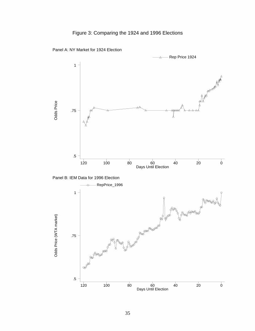
35

Figure 3: Comparing the 1924 and 1996 Elections

Panel A: NY Market for 1924 Election O

dds

Pric

e

Days Until Election

Rep Price 1924

120 100 80 60 40 20 0

.5

.75

1

Panel B: IEM Data for 1996 Election

Odd

s P

rice

(WT

A m

arke

t)

Days Until Election

RepPrice_1996

120 100 80 60 40 20 0

.5

.75

1

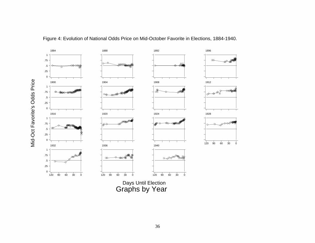
36

Figure 4: Evolution of National Odds Price on Mid-October Favorite in Elections, 1884-1940. M

id-O

ct F

avor

ite's

Odd

s P

rice

Graphs by YearDays Until Election

1884

0

.25

.5

.75

1

1888 1892 1896

1900

0

.25

.5

.75

1

1904 1908 1912

1916

0

.25

.5

.75

1

1920 1924 1928

120 90 60 30 01932

120 90 60 30 00

.25

.5

.75

1

1936

120 90 60 30 0

1940

120 90 60 30 0

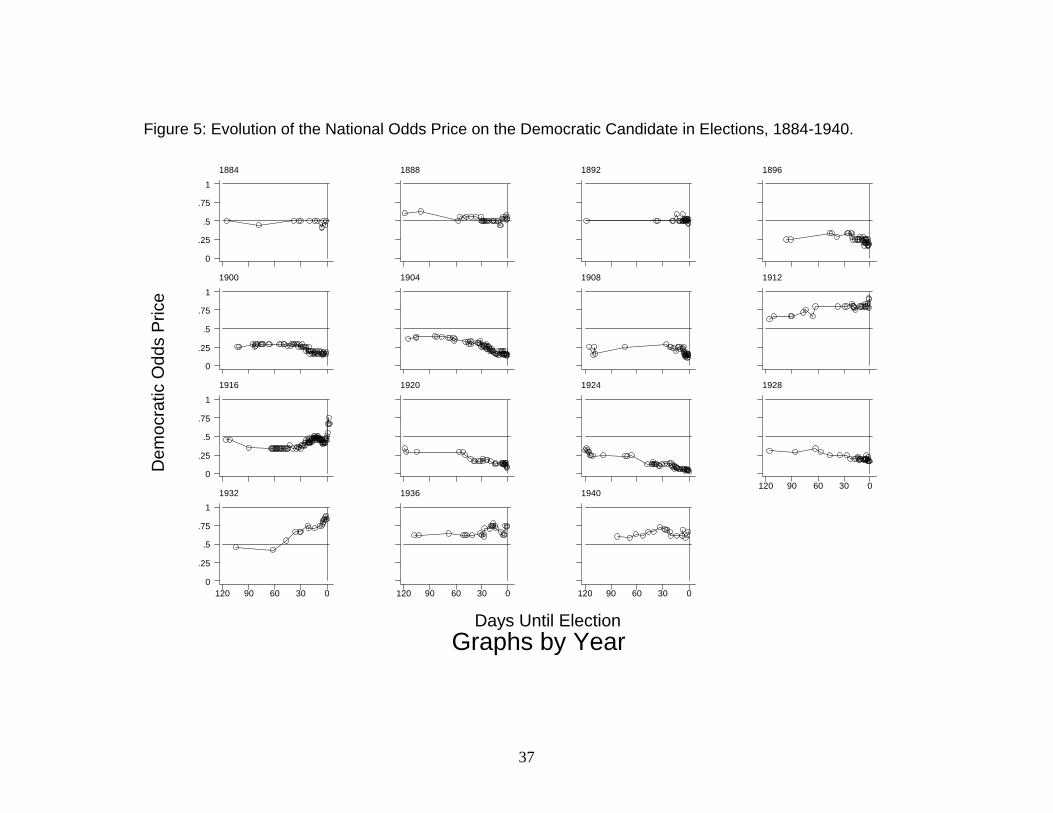
37

Figure 5: Evolution of the National Odds Price on the Democratic Candidate in Elections, 1884-1940.

Dem

ocra

tic O

dds

Pric

e

Graphs by YearDays Until Election

1884

0

.25

.5

.75

1

1888 1892 1896

1900

0

.25

.5

.75

1

1904 1908 1912

1916

0

.25

.5

.75

1

1920 1924 1928

120 90 60 30 01932

120 90 60 30 00

.25

.5

.75

1

1936

120 90 60 30 0

1940

120 90 60 30 0