hinode/eis spectroscopy and modeling · a short description of the hinode satellite and its...
TRANSCRIPT

UNIVERSITY OF OSLOInstitute of TheoreticalAstrophysics
Hinode/EISSpectroscopy andModeling
Master Thesis
Marte Elisabeth Skogvoll
June 2007


Acknowledgments
First of all I want to thank my supervisor Viggo Hansteen for guiding methrough this project. I am very grateful for the endless patience he hashad with me and my continual questions. Thanks also to Geir Emblemsvågfor helping me with all my physics and computer problems, and for proofreading my thesis.
I also want to thank Mats Carlsson, Luc Rouppe Van Der Voort andØystein Langangen for taking me to The Swedish Solar Telescope in May2006 and letting me be a ’real’ astronomer for a while.
Thanks to the people in and around IAESTE, Fysikkforeningen, andFysisk Fagutvalg for making these five years at Blindern a memorable partof my life. Especially I want to thank Josefine for being my friend and fellowstudent throughout these years. It would not have been the same withoutyou.
I want to thank Sofie, Glenn, Hanne Sigrun, Thale, Kosovare, Iselin,Stefano, Vegard, Nicolaas, and the rest of the people at Stjernekjellerenfor the interesting discussions around the lunch table. Thanks also to TheInstitute of Theoretical Astrophysics for providing such great facilities, whichhas contributed to the good professional and social environment in our studyhall.
Finally, I want to thank the rest of my friends and my family for caringand for making me think about other things than physics. Especially, I wantto thank Ivar for proof reading my thesis and for his indulgence the lastcouple of months.
Marte Elisabeth SkogvollJune 2007
iii


Contents
1 Introduction 1
1.1 The Sun . . . . . . . . . . . . . . . . . . . . . . . . . . . . . . 11.1.1 Solar Structure . . . . . . . . . . . . . . . . . . . . . . 11.1.2 The Heating Problem . . . . . . . . . . . . . . . . . . 31.1.3 Observations of the Solar Atmosphere . . . . . . . . . 4
1.2 Hinode . . . . . . . . . . . . . . . . . . . . . . . . . . . . . . . 41.2.1 Scientific Aims . . . . . . . . . . . . . . . . . . . . . . 6
1.3 The Thesis . . . . . . . . . . . . . . . . . . . . . . . . . . . . 61.3.1 Methods . . . . . . . . . . . . . . . . . . . . . . . . . . 71.3.2 Thesis Outline . . . . . . . . . . . . . . . . . . . . . . 7
2 Basic Line and Plasma Physics 9
2.1 Introduction . . . . . . . . . . . . . . . . . . . . . . . . . . . . 92.2 Electron Excitation and De-excitation . . . . . . . . . . . . . 10
2.2.1 Radiative Excitation and De-excitation . . . . . . . . . 102.2.2 Collisional Excitation and De-excitation . . . . . . . . 112.2.3 Coronal Equilibrium . . . . . . . . . . . . . . . . . . . 12
2.3 Ionization and Recombination . . . . . . . . . . . . . . . . . . 132.3.1 Collisional Ionization and 3-Body Recombination . . . 142.3.2 Photoionization and Radiative Recombination . . . . . 142.3.3 Autoionization and Dielectronic Recombination . . . . 152.3.4 The Rate Equation . . . . . . . . . . . . . . . . . . . . 16
2.4 Emission Lines . . . . . . . . . . . . . . . . . . . . . . . . . . 192.4.1 Line Profile . . . . . . . . . . . . . . . . . . . . . . . . 192.4.2 Line Momentum Analysis . . . . . . . . . . . . . . . . 192.4.3 The Emission Line Intensity . . . . . . . . . . . . . . . 21
2.5 The Hydrodynamic Plasma Equations . . . . . . . . . . . . . 232.5.1 The Conservation Equations . . . . . . . . . . . . . . . 23
3 The Simulation Code 25
3.1 The Physical Problem . . . . . . . . . . . . . . . . . . . . . . 253.1.1 Energy Sources and Sinks . . . . . . . . . . . . . . . . 263.1.2 Summary . . . . . . . . . . . . . . . . . . . . . . . . . 27
v
vi CONTENTS
3.2 TTRANZ . . . . . . . . . . . . . . . . . . . . . . . . . . . . . 283.2.1 Discretization . . . . . . . . . . . . . . . . . . . . . . . 283.2.2 Calculating the Next Time Step . . . . . . . . . . . . . 30
3.3 Input . . . . . . . . . . . . . . . . . . . . . . . . . . . . . . . . 313.3.1 The Atomic File . . . . . . . . . . . . . . . . . . . . . 313.3.2 The Init File . . . . . . . . . . . . . . . . . . . . . . . 343.3.3 The Initial Solution . . . . . . . . . . . . . . . . . . . 35
4 The Atomic Model 37
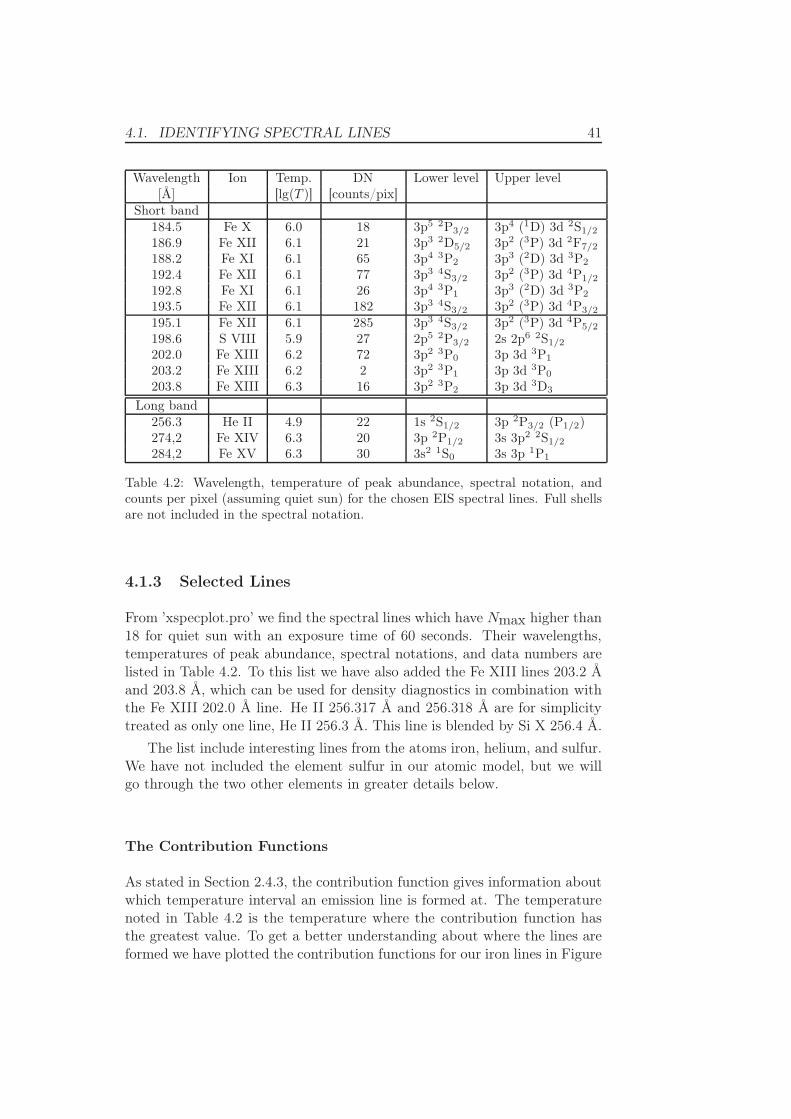
4.1 Identifying Spectral Lines . . . . . . . . . . . . . . . . . . . . 374.1.1 Resolution Requirements . . . . . . . . . . . . . . . . . 384.1.2 Estimating the Number of Counts . . . . . . . . . . . 394.1.3 Selected Lines . . . . . . . . . . . . . . . . . . . . . . . 41
4.2 Designing the Iron Model . . . . . . . . . . . . . . . . . . . . 434.2.1 Included Ions . . . . . . . . . . . . . . . . . . . . . . . 434.2.2 Included Energy Levels . . . . . . . . . . . . . . . . . 434.2.3 Particular Changes . . . . . . . . . . . . . . . . . . . . 474.2.4 Comparing the Ionization Balance . . . . . . . . . . . 48
4.3 Designing the Helium Model . . . . . . . . . . . . . . . . . . . 494.3.1 Included Ions and Levels . . . . . . . . . . . . . . . . . 494.3.2 Comparing the Ionization Balance . . . . . . . . . . . 49
5 Simulations 53
5.1 The Loop Model . . . . . . . . . . . . . . . . . . . . . . . . . 535.2 Warm Loop Cooling . . . . . . . . . . . . . . . . . . . . . . . 54
5.2.1 Loop Changes . . . . . . . . . . . . . . . . . . . . . . . 555.2.2 The EIS Lines’ Response to the Changes . . . . . . . . 595.2.3 Ionization Equilibrium . . . . . . . . . . . . . . . . . . 655.2.4 Interim Conclusion . . . . . . . . . . . . . . . . . . . . 68
5.3 Cold Loop Heating . . . . . . . . . . . . . . . . . . . . . . . . 685.3.1 Loop Changes . . . . . . . . . . . . . . . . . . . . . . . 705.3.2 The EIS Lines’ Response to the Changes . . . . . . . . 725.3.3 Ionization Equilibrium . . . . . . . . . . . . . . . . . . 775.3.4 Interim Conclusion . . . . . . . . . . . . . . . . . . . . 79
5.4 Medium Hot Loop with Waves . . . . . . . . . . . . . . . . . 805.4.1 Loop Changes . . . . . . . . . . . . . . . . . . . . . . . 815.4.2 The EIS Lines’ Response to the Changes . . . . . . . . 845.4.3 Ionization Equilibrium . . . . . . . . . . . . . . . . . . 895.4.4 Interim Conclusion . . . . . . . . . . . . . . . . . . . . 91
6 Conclusion 93
6.1 Summary . . . . . . . . . . . . . . . . . . . . . . . . . . . . . 936.2 Further work . . . . . . . . . . . . . . . . . . . . . . . . . . . 94

CONTENTS vii
Bibliography 97

viii CONTENTS
Chapter 1
Introduction
The Sun is our nearest star. By providing heat and light it sustains life onEarth and influences our climate. It is therefore interesting to understandmore about its physical processes. In addition, the Sun is important in thestudy of other stars. The Sun is an average star, and its unique locationmakes it possible to study in much greater details than the stars furtheraway. Better knowledge of the Sun improves our understanding of otherstars and astrophysical objects.
To increase our understanding of the Sun and its processes, further obser-vations are needed. In this matter, the Hinode satellite, which is the subjectof the thesis, will make valuable contributions with its studies of the solaratmosphere.
We begin the chapter by describing the structure of the Sun and one ofthe important problems solar physicists are faced with today. Then we givea short description of the Hinode satellite and its instruments. We end thechapter by describing the aim of the thesis, the methods we are using, andthe thesis outline.
1.1 The Sun
1.1.1 Solar Structure
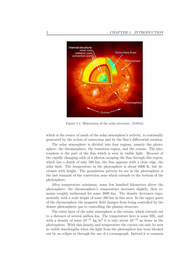
The Sun is commonly divided into two parts; the solar interior and the solaratmosphere. An illustration of the solar structure is given in Figure 1.1. Theinterior consists of a core which extends some 20 percent of the solar radius,where the hydrogen fusion is taking place. This is the process by which theSun ultimately generates its energy of 3.9 × 1026 W, and with a radius of7× 108 m this is equivalent to a flux of 6.3× 10⁷ W/m2 at the solar surface.This energy has to be transported out of the Sun, and throughout most ofthe interior this is done by radiation. In the upper 20 percent of the Sun’sradius the energy is transported by convection. The solar magnetic field,
1
2 CHAPTER 1. INTRODUCTION
Figure 1.1: Illustration of the solar structure. (NASA)
which is the source of much of the solar atmosphere’s activity, is continuallygenerated by the action of convection and by the Sun’s differential rotation.
The solar atmosphere is divided into four regions, namely the photo-sphere, the chromosphere, the transition region, and the corona. The pho-tosphere is the part of the Sun which is seen in visible light. Because ofthe rapidly changing odds of a photon escaping the Sun through this region,which has a depth of only 500 km, the Sun appears with a clear edge, thesolar limb. The temperature in the photosphere is about 6000 K, but de-creases with height. The granulation pattern we see in the photosphere isthe last remnant of the convection zone which extends to the bottom of thephotosphere.
After temperature minimum, some few hundred kilometers above thephotosphere, the chromosphere’s temperature increases slightly, then re-mains roughly isothermal for some 2000 km. The density decreases expo-nentially with a scale height of some 200 km in this area. In the upper partsof the chromosphere the magnetic field changes from being controlled by thedenser photospheric gas to controlling the plasma structure.
The outer layer of the solar atmosphere is the corona, which extends outto a distance of several million km. The temperature here is some MK, andwith a density of some 10−11 kg/m3 it is only about 10−12 as dense as thephotosphere. With this density and temperature the corona can only be seenin visible wavelengths when the light from the photosphere has been blockedout by an eclipse or through the use of a coronagraph. Instead it is common
1.1. THE SUN 3
to observe this region of the solar atmosphere in X-ray wavelengths. Herethe magnetic field expands in the increasingly tenuous plasma and fills allspace around the Sun some few thousand kilometers above the photosphere.
Between the chromosphere and the corona lies the transition region. Inthis region the temperature rises rapidly, from some 104 K to 106 K in onlya few Mm. The transition region emits most of its radiation in extremeultraviolet (EUV) spectral emission lines, mainly originating from stronglyionized metals.
The solar wind is an extension of the Sun’s atmosphere, with the highspeed electrons and ions from the corona escaping into interplanetary space.
1.1.2 The Heating Problem
As described above, the Sun’s energy is formed in the core and transportedfrom there and out to the Sun’s surface. Therefore one should expect, ac-cording to the second law of thermodynamics, that the temperature woulddecrease with distance from the Sun’s center. This is indeed the case for thesolar interior to the photosphere. From this point and upwards the oppositeis the case, the upper parts of the solar atmosphere have a much greatertemperature than the photosphere. This was shown by Edlén (1943) byidentifying forbidden lines of highly ionized atoms.
Because the corona is such a tenuous plasma the energy flux neededto heat it up to a few MK is actually quite small, only some 100 W/m2.This is only 10−6 of the radiative energy flux emerging from the Sun, whichtherefore should be more than enough to heat the corona. The lack of energyemerging from the solar interior is thus not the problem, but rather to finda mechanism that is able to transmit the energy through the photosphere,chromosphere, and transition region, and then to deposit it into the corona.This is commonly called ’the heating problem’ and has been one of the majorquestions for solar physicists the last 60 years.
Throughout the years several theories have been suggested; e.g. Bier-mann (1946, 1948) and Schwarzschild (1948) suggested that sound wavesproduced in the solar convection zone heated the chromosphere and corona,while Alfvén (1947) and Osterbrock (1961) suggested that magnetic (MHD)wave modes could carry the energy flux.
The leading idea today is that the energy transfer must be related tothe magnetic field, and possibly to the reconnection of magnetic field lines.Photospheric motions concentrate the magnetic field into small elements orpatches that are spread over the entire solar surface. In some regions, such asin sun spots or plage regions, the field becomes strong enough to dominatethe dynamics of the photosphere. Magnetic field lines are forced towardsthe inter-granular lanes because of the convection, which randomly shuff-ling them about, causing stress to build up. As the field lines become tootwisted they might snap and rearrange, causing dissipation of magnetic en-
4 CHAPTER 1. INTRODUCTION
ergy in the corona, and thus heating it (Parker, 1983). This is commonlycalled nano-flare heating by magnetic reconnection. Observational evidenceof this type of event has been found by e.g. Yokoyama et al. (2001). Inaddition, ab initio simulations by Gudiksen and Nordlund (2005) based onthis idea, starting from a prescribed photospheric velocity field and observedphotospheric magnetic field, generate coronal structures very similar to thoseobserved. Even so, the answer to the heating problem is still not fully un-derstood, and further observations are needed to better understand the roleof the magnetic field in the coronal heating. To determine how the energy istransferred from below the photosphere and up into the outer atmosphere,we need to simultaneously measure the changes in the magnetic field andthe emission lines’ intensities from the transition region and corona.
1.1.3 Observations of the Solar Atmosphere
Since the recognition of the high temperatures in the upper solar atmospherethere has been a need for better observations of this region. As describedabove, the transition region and the corona emit most of their radiationin EUV and X-ray wavelengths, respectively. The Earths atmosphere isopaque to these wavelengths, so to be able to observe these regions in thewavelengths they are emitting strongest, the detector must be sent up aboveour atmosphere.
There have been several successful rocket and satellite experiments sofar, e.g. Orbiting Solar Observatory, Skylab, Spacelab 2, and in later timesthe Solar and Heliospheric Observatory (SOHO) and Transition Region andCoronal Explorer (TRACE).
1.2 Hinode
The Japanese Hinode (Solar-B) (Ichimoto and Solar-B Team, 2005), thesuccessor to YOHKOH (Solar-A) mission, was launched 22 September 200621:36 UT. It studies the Sun in visible, EUV, and X-ray wavelengths, inaddition to being able to produce vector magnetogram maps. The satel-lite is moving in a 680 km circular Sun-synchronous orbit over the Earth’sday/night terminator, which allows near-continuous observation of the Sun.Each orbit takes 96 minutes, which yields 15 orbits a day. Data is broughtdown at a number of ground stations, including at the Uchinoura SpaceCentre in Japan and at KSAT’s Svalbard Station. This allows at least 17daily ground station contacts, and thus an average of 6 Gbytes data telemetrya day. Hinode carries three instruments; a Solar Optical Telescope (SOT), anX-ray Telescope (XRT) and an EUV Imaging Spectrometer (EIS). A shortdescription about each of them are given below.

1.2. HINODE 5
SOT
SOT (Ichimoto et al., 2004) consists of two major components; namely theOptical Telescope Assembly (OTA) and the Focal Plane Package (FPP).OTA is with its 50 cm, the largest optical solar telescope that has everbeen sent out into space. It has a wavelength coverage of 3870–6680 Å(visible light), and will thus observe the photosphere and chromosphere. Ithas a resolution of 0.25 arc seconds, which means that details down to 175km can be resolved on the Sun. The light captured by SOT is analyzedin the FPP consisting of three instruments; a Narrowband Filter Imager(NFI), a Broadband Filter Imager (BFI) and a Spectropolarimeter (SP).NFI can compute the four Stokes parameters and Dopplergrams (line-of-sight velocity) of the photosphere and chromosphere. BFI produces highspatial and temporal resolution images and measures horizontal flow andthe temperature in the photosphere. With the polarized spectra from SPone can produce photospheric 3D vector magnetograms.
XRT
XRT (Kano et al., 2004) is a high resolution grazing incidence telescope,and its goal is to observe the high temperature plasma of the corona. Byproducing images with different X-ray filters, XRT can observe in a widertemperature band (1–30 MK) than previous X-ray telescopes. This allowsfor detections of dissipation of magnetic energy in forms of flares and coronalmass ejections. XRT can either observe the full solar disk or a smaller areawith higher resolution. XRT is expected to have an angular resolution of 2arc seconds, or about 1400 km on the Sun. Built-in visible light optics allowfor sub-pixel accuracy image alignment with SOT.
EIS
EIS (Culhane et al., 2007) is an EUV spectrometer which can observe variouslines in two wavelength intervals, 170–210 Å and 250–290 Å, covering a widerange of plasma temperatures (0.1–20 MK). With the spectra from EIS it ispossible to determine the intensity, the Doppler velocity, the line width, andthe temperature and density of the plasma where the line is formed.
Due to the use of multi-layer coated optics and back-illuminated CCDs,EIS has approximately a factor 10 enhancement in effective area comparedto CDS (on board SOHO). In addition, the spectral resolution (3 km/s forDoppler velocities) is also improved by an order of magnitude, and the spatialresolution (2 arc seconds) is improved by a factor two or three compared toCDS.

6 CHAPTER 1. INTRODUCTION
1.2.1 Scientific Aims
The scientific aims of the Hinode mission are focused on three main goals:
• To determine the mechanisms responsible for heating the corona inactive regions and the quiet Sun.
• To establish the mechanisms responsible for transient phenomena, suchas flares and coronal mass ejections.
• To investigate the processes responsible for energy transfer from thephotosphere to the corona.
These goals will be approached by using the combination of the threedifferent instruments on board the satellite. By observing the photosphereand the underlying magnetic field at the same time as the chromosphere andcorona, one gets a better possibility of understanding the connection betweenthe different parts of the Sun. In particular, it is interesting to observe thedynamic and thermal response of the corona to the changing magnetic andvelocity fields of the photosphere and convection zone, to see if we can getcloser to the answer to the heating problem.
1.3 The Thesis
The aim of the thesis is to better understand how we can relate the EIS ob-servations to physical phenomena in the solar atmosphere. Specifically, wewant to study how the diagnostic variables react to changes in the morpho-logy in the solar atmosphere. That is, we will study how the line intensityand the Doppler velocity for the spectral lines observable with EIS react tothe changes in temperature, density, and velocity. Especially, we want tostudy the iron lines formed in the corona around 1 MK, and examine whatthey can tell us about the condition in the upper solar atmosphere.
Since we can not ’check’ what is really happening when there is an eventon the Sun for then to see how the EIS lines respond to these, we approachthis problem by numerical simulations. We make a model of the solar atmo-sphere, introduce perturbations to this system, and examine how the proper-ties of the gas change according to these events. Then we study how the EISemission lines change as a result of this perturbation. Thereafter, we discusswhich of these changes EIS is actually able to detect, and whether observingwith EIS can explain the physical phenomena causing these changes.
EIS is only able to detect the emission line intensity, Doppler velocity,and line width. In addition, one can also compute the temperature anddensity in the region where the line is formed. These temperature and dens-ity diagnostics are only reliable as long as the line is formed in ionizationequilibrium. Therefore, we also examine whether any of our spectral linesare driven out of equilibrium during our simulations.

1.3. THE THESIS 7
By following this procedure we can come to a better understanding ofwhich phenomena EIS is able to detect, which limitations the data have,and which cautions must be taken when drawing conclusions from the EISobservations to the physical explanations about what is actually happening.Thus we find out how to better use the EIS data.
1.3.1 Methods
To solve this problem we use a combination of the simulation code TTRANZ
(Hansteen, 1991) and the IDL package CHIANTI (Landi et al., 2006; Dereet al., 1997). TTRANZ solves the hydrodynamic plasma equations in onedimension along with the rate equations which determine the radiative lossesfrom the transition region and corona. CHIANTI is an atomic database andcontains routines for exploitation of this data.
A schematically overview of the work is given by:
1. Identifying the most important EIS spectral emission lines by usingthe CHIANTI atomic database.
2. Constructing usable TTRANZ atomic data files, using the CHIANTIatomic database, the HAO-DIAPER package (Judge and Meisner,1994), and the NIST line database (Ralchenko et al., 2005) as refer-ences.
3. Constructing a coronal loop model and examining how this reacts toperturbations, such as changes in the heating rate and forced waves onthe system.
4. Examining how the chosen EIS spectral lines’ intensities and velocitiesreact to the loop changes.
5. Examining whether any of the chosen EIS spectral lines are driven outof ionization equilibrium in the scenarios described above.
1.3.2 Thesis Outline
The remainder of this thesis is divided into five chapters. We start by goingthrough the basic physics behind emission line formation and the hydro-dynamic plasma equations in Chapter 2. Further, in Chapter 3 we describeour simulation code, explain the numerical schemes in use, and how inputare given to the program. In Chapter 4 we examine the performance of theEIS spectrograph and decide which emission lines in the EIS passband thatare usable for our purpose. In this chapter we also design the atomic modelsneeded. In Chapter 5 we run our simulation code with the input found in theprevious chapters. We perturb the system by changing the heat input and

8 CHAPTER 1. INTRODUCTION
forcing waves on the system, and analyze the changes in the loop morpho-logy. Thereafter, we examine the diagnostic variables for the chosen lines tosee if they can explain the loop changes. Finally, in Chapter 6 we summarizewhat we have done and which results we have come to and give suggestionsfor further work and improvements.
Chapter 2
Basic Line and Plasma Physics
In this chapter we first give an introduction to what an emission line is.Thereafter, we go through the different processes that contribute to theemission line formation and the processes that determine the ionization stateof an element. Then we explain how we can compute the emission lines’intensity and Doppler velocity. Finally, we give a short introduction to thehydrodynamic plasma equations, which describe the behavior of the plasmain the solar atmosphere.
2.1 Introduction
The solar atmosphere consists of a warm and low density gas. Below liesthe cooler and denser photosphere, which radiates as a black body with itsemission peak in the visible wavelength interval. Therefore, the atmosphereis most easily observed in the short wavelength part of the spectrum, whereits emission lines out-shine the continuum.
Emission lines are caused by photons emerging from the solar atmospherewhen an ion de-excites from an excited upper energy level ’u’ to a lowerenergy level ’l’. The energy taken away by the photon is given by the energydifference of the two levels,
∆E = Eu − El = hν , (2.1)
where h is the Planck constant, ν is the frequency, and Eu and El are theenergies of the upper and lower levels, respectively.
The gas is considered optically thin when all the emitted photons leavethe atmosphere without being scattered, and effectively thin if all createdphotons eventually escape after a number of scatterings before being thermal-ized. The intensity Iν of an optically thin spectral emission line with fre-quency ν is related to the number density of ions in the correct upper energy
9

10 CHAPTER 2. BASIC LINE AND PLASMA PHYSICS
level (nu), and the rate at which these de-excite by emitting a photon (Aul).
Iν =hν
4π
∫ s
0nuAul φν ds , (2.2)
where we have divided by the sphere solid angle unit since the photon canbe sent out in any direction, and integrated along the line of sight s. φν isthe line’s emission profile which we will come back to in Section 2.4.1.
To compute the intensity we thus have to find expressions for our twounknowns nu and Aul. These are both related to the ion’s excitation andde-excitation processes which we discuss in Section 2.2.
2.2 Electron Excitation and De-excitation
Electron excitation is the process in which a bound electron transfers froma low lying energy level ’l’ (ground or excited) to a higher energy level ’u’by stealing energy from a photon or a free electron. The inverse process iscalled electron de-excitation, and take place when a bound electron transfersfrom an excited energy level to a lower lying level (ground or excited) andthe extra energy is taken away either by a photon or a free electron.
Bound-bound transitions between two levels can occur in different ways,and we will give a short introduction to each of them:
• radiative excitation and de-excitation (photoabsorption, spontaneousradiative de-excitation, and stimulated emission) (Section 2.2.1)
• collisional excitation and de-excitation (Section 2.2.2)
2.2.1 Radiative Excitation and De-excitation
Absorption is the process in which an ion absorbs a free photon and becomesexcited up into a higher energy level. The rate coefficient for this process isdenoted Blu. The inverse process, called spontaneous radiative de-excitation,is the process where an excited atom decays into a lower level, and thus emitsa photon which carries away the energy difference between the two levels.Its rate coefficient is denoted Aul.
Xl + hν ⇔ Xu , (2.3)
where Xl and Xu denote the lower and upper energy levels, respectively.The principle of detailed balance states that in thermal equilibrium (TE)
the number of transitions due to one process is exactly balanced by its inverseprocess. To meet this requirement of TE, we need a third process, namelystimulated emission, with rate coefficient Bul. In this process a photon hitsan excited atom, which then de-excites and sends out another photon,
Xu + hν ⇒ Xl + hν + hν . (2.4)
2.2. ELECTRON EXCITATION AND DE-EXCITATION 11
These three rate coefficients are all called Einstein coefficients, and arerelated by
Bul
Blu=
ωl
ωu, (2.5)
where ωu and ωl are the multiplicities (statistical weights) for the upper andlower levels, respectively, and
Aul
Bul=
2hν3
c2, (2.6)
where c is the speed of light in vacuum. These two relations hold universallysince they do not depend on any property of the medium.
The spontaneous de-excitation rate is in the literature often given by theoscillator strength (ful), which is related to the Einstein A coefficient by(Rutten, R. J., 2003),
Aul = 6.671 × 10¹⁵ ωl
ωu
ful
λ2, (2.7)
with λ in Å.
2.2.2 Collisional Excitation and De-excitation
A free electron that moves close to an ion can transfer some of its energyto one of the bound electrons. The free electron loses the same amount ofenergy as it takes to excite the bound electron from a lower level ’l’ into anupper level ’u’. The transition rate for collisional excitation is denoted Clu.In the inverse process an electron hits an excited atom, the bound electronde-excites to a lower level and the free electron takes away the extra energy.The rate coefficient for this process is denoted Cul. These processes are alsocalled electron impact excitation and electron impact de-excitation.
Xl + e ⇔ Xu + e (2.8)
The collisional excitation rate coefficient is related to the collision crosssection (σ) of the collision between the ion and electrons of velocity u.
Clu =
∫ ∞
u0
σlu(u)f(u)u du , (2.9)
where the threshold energy is given by 12meu
20 (me is the electron mass)
and f is the velocity distribution function of the electrons. The collisioncross section can be found either by theoretical calculations or in laboratoryexperiments.
Assuming that the electron distribution function is Maxwellian, we canwrite the collision rate as a function of the temperature alone (Mason andFossi, 1994),
Clu(Te) =C0
ωlT−1/2
e e−∆E/kBTeΥlu(Te) , (2.10)
12 CHAPTER 2. BASIC LINE AND PLASMA PHYSICS
where ωl is the multiplicity of the lower level, C0 = 8.63×10⁻⁶ is a constant,kB is the Boltzmann constant, and Te is the electron temperature. Υlu isthe thermally averaged collision strength, which is a slowly varying functionwith temperature.
The rate coefficients for the collisional excitation and de-excitation pro-cesses are related through the detailed balance principle,
Clu
Cul=
ωu
ωle−∆E/kBTe . (2.11)
This relation also holds outside TE, as long as the electron velocity distri-bution function is Maxwellian.
2.2.3 Coronal Equilibrium
We have now given an overview of the different excitation and de-excitationprocesses that can occur. We are interested in the region of the solar at-mosphere where the extreme ultraviolet (EUV) radiation is emitted. In thisregion the electron density is low (ne < 1018 m−3) and the temperature ishigh (Te > 104 K). This leads to the so-called Coronal Equilibrium (CE)condition, which allows us to do some simplifications.
Excitation – De-excitation Rate Equation
With CE conditions it is usually safe to assume that the population of theupper level mainly is produced by collisional excitation from the groundlevel, and that the spontaneous radiative decay overwhelms the other de-population processes. The number of excitations and de-excitations mustbalance each other, so we get the simple relation
nuAul = nlneClu . (2.12)
This approximation is not correct if there is no allowed transition (ac-cording to the electric dipole approximation) down from the excited state’u’. If this is the case, the spontaneous radiative de-excitation rate is quitesmall and the collision de-excitation rate becomes comparable to it. Thiskind of upper level is called a meta-stable level, and extra attention must begiven to these levels when designing our atomic model.
Assuming Equation 2.12 to be valid, another expression for the unknownparameters in Equation 2.2 (nuAul) are found. In the previous section wealso found an expression for the collision excitation rate (Equation 2.10), soour challenge is now to find the number density of ions in the lower energylevel, nl.
2.3. IONIZATION AND RECOMBINATION 13
Number Density
Within CE we can assume that the de-excitation rates are much higher thanthe excitation rates. As noted above, this is not the case for meta-stablelevels, which can cause a notable amount of the ions to not be in the groundstate.
Without meta-stable levels the number of ions in the low-energy level canbe considered the same as the total number of ions in the ionization state.
nl(Xm) ≈ n(Xm) , (2.13)
where Xm represent the ionization state m, and the subscript ’l’ denotes theexcitations level, which is normally the ground level. We can express thenumber of ions in the lower level as
nl(Xm) =
(
n(Xm)
n(X)
)(
n(X)
nH
)
nH , (2.14)
where the first ratio is the fraction of the element in the correct ionizationstate and the second is the element abundance relative to hydrogen,
n(X)
nH= Ab . (2.15)
This abundance can, as a first approximation, be considered constant throughthe solar atmosphere. The ionization fraction on the other hand, varies a lotaccording to the temperature and density. We examine the ionization andrecombination processes in Section 2.3.
2.3 Ionization and Recombination
It is the bound-free and free-bound processes that make an atom trans-fer from one ionization stage to the next as the surrounding environmentchanges. The ionization state is found by solving the rate equation,
∂n(Xm)
∂t+
∂
∂z(n(Xm)u) = Sources − Sinks . (2.16)
We will take a look at the ionization and recombination processes, which canbe both sources and sinks:
• collisional ionization and 3-body recombination (Section 2.3.1)
• photoionization and radiative recombination (Section 2.3.2)
• autoionization and dielectronic recombination (Section 2.3.3)

14 CHAPTER 2. BASIC LINE AND PLASMA PHYSICS
2.3.1 Collisional Ionization and 3-Body Recombination
In collisional ionization, also called electron impact ionization, a free electronhits an atom and knocks free a bound electron. In the recombination processtwo free electrons enter at the same time into the volume of the ion, one ofthem is captured in an excited energy level while the other carries away theextra energy.
Xmi + e ⇔ Xm+1
j + e + e (2.17)
where m is the ionization state and i, j are the excitation levels.As for the collisional excitation, the collisional ionization rate Icol is re-
lated to the collisional ionization cross section (σ). The total number ofionizations because of this process is given by
I(col)neni(Xm) = neni(X
m)
∫ ∞
u0
σ(u)f(u)u du , (2.18)
where the threshold energy is given by 12meu
20 and f is the electron velocity
distribution function.The 3-body recombination rate is denoted R(3). This rate is because of
the detailed balance principle related to the collisional ionization rate by theSaha equation (Mihalas, 1978);
(
ni(Xm)
nj(Xm+1)
)∗
= C1neωm
ωm+1T−1.5e
E(Xm+1)−E(Xm)kBTe , (2.19)
where C1 = 2.07×10⁻¹⁶ (in cgs units) and the superscript ’∗’ denotes thermalequilibrium. The total number of recombinations due to the 3-body processis given by
R(3)nenj(Xm+1) = nenj(X
m+1)I(col)
(
ni(Xm)
nj(Xm+1)
)∗
. (2.20)
This holds also outside of TE as long as the velocity is Maxwellian.Since the 3-body recombination requires the presence of two electrons
at the same time, this rate is quite small for low density plasma, where thecollisional ionization is the dominant ionization process.
2.3.2 Photoionization and Radiative Recombination
In photoionization a photon is absorbed by a bound electron which thenbreaks free from the atom. In the inverse process, radiative recombination, afree electron is captured by a ’bare’ ion while a photon takes away the extraenergy.
Xm+1j + e ⇔ Xm
i + hν (2.21)
2.3. IONIZATION AND RECOMBINATION 15
The total number of ionizations because of photoionizations is given by
I(ph)ni(Xm) = ni(X
m)4π
∫ ∞
ν0
α(ν)
hνJν dν , (2.22)
where α is the photoionization cross section and Jν is the mean intensity.Note that I(ph) is a function of the radiation temperature and that the totalnumber of transitions of this kind do not depend on the electron density.
In TE the number of spontaneous recombinations must equal the numberof photoionizations
R(r)
(
nj(Xm+1)
)∗= I(ph) (ni(X
m))∗ . (2.23)
The total number of radiative recombinations is therefore given by
R(r)nenj(Xm+1) =nenj(X
m+1)
(
ni(Xm)
nj(Xm+1)
)∗
×
4π
∫ ∞
ν0
α(ν)
hνBν dν ,
(2.24)
where the mean intensity is given by the Planck function (Jν = Bν) in TE.This rate also holds when TE is not valid as long as the velocity distributionis Maxwellian.
The photoionization is negligible in optically thin plasma, because thereare very few photons with enough energy to ionize the atom, while the radi-ative recombination, on the other hand, is the main recombination process.
2.3.3 Autoionization and Dielectronic Recombination
We can have a spontaneous ionization in a doubly excited atom if the energyof the lowest excited electron is larger than the binding energy of the otherexcited electron. This is called autoionization. The inverse process is of twosteps. First, a free electron is captured into an excited state of the ion andanother bound electron takes up the rest energy, and becomes excited too.This is the opposite of autoionization. To have dielectronic recombinationwe also need the second step; at least one of the two excited electrons goesthrough a radiative decay and sends out a photon.
Xm+1g + e ⇔Xm
ij
Xmij → Xm
gj + hν(2.25)
Here g refers to the ground level and i, j to excited levels.Recall from the discussion of coronal equilibrium that most of the atoms
are in their ground states, so the autoionization process can not happenvery often. The dielectronic recombination on the other hand, happens quitefrequently in hot, low density plasma.
16 CHAPTER 2. BASIC LINE AND PLASMA PHYSICS
The dielectronic rate coefficient R(d) is a function of the electron temper-ature, and the total numbers of recombinations of this kind is given by
R(d)neng(Xm) . (2.26)
2.3.4 The Rate Equation
In the beginning of this section we stated the general rate equation (Equation2.16), and we have now outlined its sources and sinks to see which of themthat play an important role in our model. We found that in the transitionregion ionization is dominated by electron impact, and recombinations aredominated by radiative and dielectronic processes. We can thus simplify therate equation by choosing R = R(r) + R(d) and I = I(col). Further, if the lefthand side of the rate equation is negligible, it is even more straightforward.It is negligible when the perturbation time scales are long compared to therate characteristic times, which are in the order of tens of seconds. We canthen set the left hand side of Equation 2.16 to zero and the sources and sinkshave to balance each other,
ne
[
n(Xm−1)Im−1 + n(Xm+1)Rm+1]
= ne [n(Xm)(Im + Rm)] . (2.27)
If we want to study effects that have shorter time scales than the rate char-acteristic time, we need to include the left hand side of the rate equationtoo.
Example: The Ionization Balance for Hydrogen
To clarify the concept of the rate equation we will solve it for the simplestcase, that is, hydrogen with only two allowed states, neutral hydrogen withnumber density nHI and ionized hydrogen with number density nHII . Wewill study how the ionization fraction reacts to changes in the temperat-ure and electron density, and relate this to the changes in the ionizationand recombination rates. We also check if it is reasonable to ignore 3-bodyrecombination, and if TE is a good approximation in the transition region.
The hydrogen atom does not have two electrons, so we can not havedielectronic recombination or autoionization. The rate equation for this sys-tem is thus given by
nHIIne
[
R(r) + R(3)
]
= nHI
[
I(col)ne + I(ph)
]
, (2.28)
which can be rewritten
nHI
nHII=
R(r) + R(3)
I(col) +I(ph)
ne
. (2.29)

2.3. IONIZATION AND RECOMBINATION 17
This is one equation with two unknowns, so we need one more equation tosolve our problem. We can use the fact that the total number of hydrogenatoms must be constant,
nHI + nHII = nH . (2.30)
The fraction of ionized hydrogen to the total number of hydrogen atomsis thus given by
nHII
nH=
(
1 +nHI
nHII
)−1
=
1 +R(r) + R(3)
I(col) +I(ph)
ne
−1
. (2.31)
To be able to solve this equation we need expressions for the different ratesthat are involved. The following expressions are taken from a hydrogenatomic model made by P. Judge for V. Hansteen in 1995. It includes atomicdata from (Janev et al., 1987) as given by the HAO-DIAPER package(Judge and Meisner, 1994).
The Collisional Ionization Rate
I(col)(Te) = T 1/2e e−hν/kBTeΥ(Te) (2.32)
with Υ being a slowly-varying function of Te, with values around 4.2×10⁻¹¹.
The Photoionization Rate
I(ph)(Trad) =8πα(ph)g(ph)ν3
c2E1
(
hν
kBTrad
)
(2.33)
where α(ph) = 7.9 × 10⁻¹⁸, g(ph) = 0.8 is the gaunt factor, and E1 isthe exponential integral.
The Radiative Recombination Rate
R(r)(Te) = α
(
Te
1 × 10⁴
)−ǫ
(2.34)
where α = 4.25 × 10⁻¹³ and ǫ = 0.69.
The 3-Body Recombination Rate
R(3)(Te, ne) = Icol × 2.07 × 10⁻¹⁶neωHI
ωHIIT−1.5
e ehν/kBTe (2.35)
where the multiplicities are ωHI = 2 and ωHII = 1.
18 CHAPTER 2. BASIC LINE AND PLASMA PHYSICS
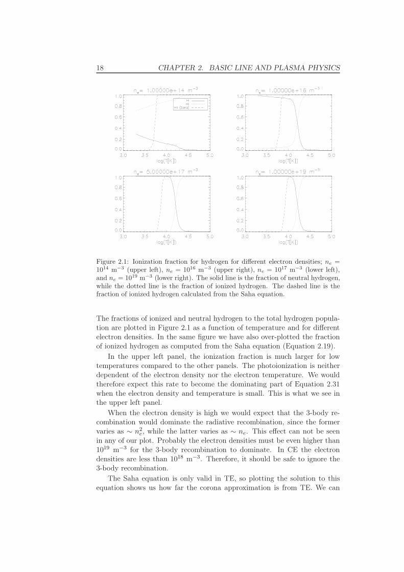
Figure 2.1: Ionization fraction for hydrogen for different electron densities; ne =1014 m−3 (upper left), ne = 1016 m−3 (upper right), ne = 1017 m−3 (lower left),and ne = 1019 m−3 (lower right). The solid line is the fraction of neutral hydrogen,while the dotted line is the fraction of ionized hydrogen. The dashed line is thefraction of ionized hydrogen calculated from the Saha equation.
The fractions of ionized and neutral hydrogen to the total hydrogen popula-tion are plotted in Figure 2.1 as a function of temperature and for differentelectron densities. In the same figure we have also over-plotted the fractionof ionized hydrogen as computed from the Saha equation (Equation 2.19).
In the upper left panel, the ionization fraction is much larger for lowtemperatures compared to the other panels. The photoionization is neitherdependent of the electron density nor the electron temperature. We wouldtherefore expect this rate to become the dominating part of Equation 2.31when the electron density and temperature is small. This is what we see inthe upper left panel.
When the electron density is high we would expect that the 3-body re-combination would dominate the radiative recombination, since the formervaries as ∼ n2
e, while the latter varies as ∼ ne. This effect can not be seenin any of our plot. Probably the electron densities must be even higher than1019 m−3 for the 3-body recombination to dominate. In CE the electrondensities are less than 1018 m−3. Therefore, it should be safe to ignore the3-body recombination.
The Saha equation is only valid in TE, so plotting the solution to thisequation shows us how far the corona approximation is from TE. We can
2.4. EMISSION LINES 19
see that our results are getting closer to the Saha solution as the density isincreasing, but clearly TE is not a good approximation for the densities weare interested in.
2.4 Emission Lines
So far we have discussed details about the atomic processes which contributeto emission line formation. It is now time to look at the observed emissionline. First we explain how to compute the line intensity, Doppler velocity,and line width. Then we take a new look at how to compute the emissionline intensity, and define the contribution function and branching fraction.At the end we collect the threads to get a better understanding of whichplasma parameters that are important in the study of emission lines.
2.4.1 Line Profile
Emission lines are not, despite their names, infinitely thin lines but are inreality smeared out according to a line profile. The emission profile due tothermal Doppler broadening is given by
φν =1√
πwDexp
[
−(
∆ν − uc ν cos θ
wD
)2]
, (2.36)
where ∆ν = ν − ν0 is the distance from the laboratory frequency, θ is theaspect angle, u is the gas velocity, and the Doppler width is given by
wD =ν0
c
√
2kBTe
mA, (2.37)
where mA is the mass of the radiating ion.
2.4.2 Line Momentum Analysis
The line’s intensity, velocity and width are not the same throughout the solaratmosphere. We therefore have to perform a column-integration to find thevalues that we would observe with a spectrograph. A powerful way of doingthis is momentum analysis.
Line Intensity
The total line intensity at a wavelength can be found by integrating theintensities at each depth point along the loop (z),
Iν =
∫ z
0Iν(z) dz . (2.38)

20 CHAPTER 2. BASIC LINE AND PLASMA PHYSICS
Doppler Velocity
Because of relative velocities between the gas and the observer the lines areshifted according to the Doppler effect,
ν = ν0
(
1 +u
c
)
, (2.39)
where u is the velocity difference between the gas and the observer. We arehere assuming motion along the line of sight only, and that the velocity issmall compared to the speed of light.
The first moment,
M1 = ∆ν =
∫
Iν(ν − ν0)dν∫
Iνdν, (2.40)
defines the mean line shift. This can be transformed to the mean velocity〈u〉 by
〈u〉 =∆ν
ν0c . (2.41)
Line Width
As mentioned above, thermal Doppler broadening is one of the processesthat increases the line width. When calculating the line width it is commonto use the standard deviation,
〈wν〉 = σ =√
M2 − M21 , (2.42)
where the subscript ’ν’ means that the width is measured in frequency, andthe second moment is given by
M2 =
∫
Iν(ν − ν0)2dν
∫
Iνdν. (2.43)
The line width can also be expresses as a function of wavelength, by using
∆λ ≈ c∆ν
ν20
, (2.44)
so that we get〈wλ〉 = c
wν
ν20
. (2.45)
By using equation 2.37 we can express the line width as a function of tem-perature,
〈wT 〉 =
(
cwν
ν0
)2 mA
2kBTe. (2.46)
2.4. EMISSION LINES 21
2.4.3 The Emission Line Intensity
We started this chapter by giving an expression for the emission line intensity,Equation 2.2,
Iν =hν
4π
∫ s
0nuAul φν ds .
Then we discussed the processes which contribute to emission line formationand found that in CE we can substitute Equation 2.12 and 2.14 into thisexpression. The emission line intensity is then given by
Iν =hν
4πAb
∫ s
0
n(Xm)
n(X)nenHCluφνds . (2.47)
It is not intuitive from this expression which variables we need to know tobe able to compute the emission line intensity. Let us therefore define somefunctions which include some of these parameters, and write explicitly whichvariables they depend on.
Contribution Function
The contribution function is defined as
G(Te, ne) =n(Xm)
n(X)Clu . (2.48)
Since both the ionization fraction and the collision rate are dependent onthe electron temperature (see Equation 2.10 and Section 2.3.4), so is thecontribution function. Actually, it is strongly dependent on the temperatureand weakly dependent on the electron density. The contribution functiongives information about which temperature regimes in the stellar atmospherethat contribute to the emission line. A plot of the contribution functionfor two iron lines (Fe XI 188.2 Å and Fe XV 284.2 Å) and one sulfur line(S VIII 198.6 Å) made using the CHIANTI (Dere et al., 1997; Landi et al.,2006) function ’ch_synthetic’ can be seen in Figure 2.2. Clearly the S VIIIline originate at the coldest temperature regime, the Fe XI line at a warmer,and the Fe XV line at an even hotter temperature regime of the atmosphere.The contribution function is very narrow, thus we only need to consider afew dex1 on each side of the temperature maximum, to include the regimewhere this function is non-zero.
Differential Emission Measure
We can also define the differential emission measure,
DEM(Te) = nenHds
dTe. (2.49)
1Dex is a measure of the difference in logarithmic values. E.g. the difference between10
5.5 and 105.6 is one dex.

22 CHAPTER 2. BASIC LINE AND PLASMA PHYSICS
Figure 2.2: The contribution function for three UV lines, Fe XI 188.2 Å (solid),Fe XV 284.2 Å (dotted), and S VIII 198.6 Å (dashed).
The DEM gives an indication of the amount of plasma along the line ofsight (s) that is emitting the radiation observed and has a temperaturebetween Te and Te + dTe.
The Branching Fraction
In Equation 2.2 we could also have included the branching fraction (Brul).This is a correction term that should be included if the electron has morethan one lower level it can de-excite to. The branching fraction is the fractionof the ions that actually de-excites to the desired lower level, and is defined
Brul =Aul
∑
k Aukk < u , (2.50)
where Auk are the de-excitation rates for the different possible transitionsfrom level ’u’.
Computing the Emission Line Intensity
By using our newly defined functions, the intensity can be written
Iν =hν
4πAb
∫
∆TG(Te, ne)DEM(Te)φdTe , (2.51)
where ∆T is the area where the contribution function is non-zero as explainedabove. The first part of this expression is as a first approximation considered
2.5. THE HYDRODYNAMIC PLASMA EQUATIONS 23
constant through the solar atmosphere, while the contribution function andDEM are functions of the electron density and temperature. To compute theemission line intensity we thus need to know how the electron temperature(Te) and the density (ne, nH) vary as functions of time (t) and height (z).That is, we need to solve the hydrodynamic plasma equations.
2.5 The Hydrodynamic Plasma Equations
When describing the flow of plasma and gases it is common to use the hy-drodynamic equations characterized by the density (ρ), velocity (u), andinternal energy (e). We are actually interested in the temperature, which isrelated to the internal energy, e ∝ ρTe.
We assume the magnetic field to be strong, that is that the tension inthe magnetic field pB (a magnetic analogous to pressure) is much strongerthan the pressure pg,
β =pg
pB=
2µ0nkBT
B2≪ 1 , (2.52)
where µ0 = 4π×10−7 H/m is the magnetical permeability of empty space, nis the particle number density, and B is the magnetic field strength. Whenthis is the case the plasma dynamics have to follow the magnetic field lines,and it is safe to restrict our calculations in one dimension along the magneticfield.
We consider a transition region flux tube with length z of time independ-ent area, A(z) = constant, and assume the atmosphere to be homogeneousin the direction normal to z within the tube.
2.5.1 The Conservation Equations
As stated above, in a low-β plasma we can use the conservation equationsin one spatial dimension.
Conservation of Mass
∂ρ
∂t+
∂
∂z(ρu) = 0 (2.53)
This equation state that there are no sources or sinks for matter.
Conservation of Momentum
ρ∂u
∂t+ ρu
∂u
∂z= − ∂
∂z(p + Q) − ρg‖ , (2.54)
where g‖ is the absolute value of the component of gravity parallel with themagnetic field, and the pressure is given by the ideal gas law,
p =ρkBT
m. (2.55)

24 CHAPTER 2. BASIC LINE AND PLASMA PHYSICS
To ensure a continuous solution through the shocks that may develop, weadd an artificial viscous pressure (von Neumann and Richtmyer, 1950).
Q =
{
43ρl2 (∂u/∂z)2 for (∂u/∂z) < 00 for (∂u/∂z) ≥ 0
, (2.56)
where l is chosen to be some fraction of the average grid spacing.
Conservation of Energy
∂
∂t(ρe) +
∂
∂z(ρue) + (p + Q)
∂u
∂z=
∂
∂z(Fc + Fr + Fh) , (2.57)
where the internal energy (e) is the sum of the thermal and ionization energyand the source and sink terms on the right hand side are:
• the conductive flux (Fc)
• the radiative losses (∂Fr/∂z)
• the heating function (Fh)
We give more details about how these are computed in Section 3.1.1.
Chapter 3
The Simulation Code
In this chapter we give an introduction to our numerical analysis. First weexplain what our problem is and why the solution has to be found numer-ically. Then we examine how our simulation code computes the solution toour problem. Finally, we describe how input is given to the program.
3.1 The Physical Problem
The aim of the thesis is to examine how the intensity and Doppler velo-city of the emission lines detected by EIS respond to changes in the solaratmosphere. The intensity is computed from Equation 2.47
Iν =hν
4πAb
∫ s
0
n(Xm)
n(X)nenHCluφνds .
As we discussed in Section 2.3, the ionization fraction n(Xm)n(X) is determined
by the rate equation (Equation 2.16),
∂n(Xm)
∂t+
∂
∂z(n(Xm)u) = Sources(Te, ne) − Sinks(Te, ne) .
The sources and sinks in this equation are determined by the electron tem-perature and to a smaller degree by the electron density. How these para-meters vary as a function of time and space are described by the conservationequations.
As explained in Section 2.5, we consider the magnetic field to be strong,β ≪ 1, which restricts the plasma to follow the magnetic field lines. Thuswe can use the one dimensional conservation equations given by Equations2.53, 2.54, and 2.57:
∂ρ
∂t+
∂
∂z(ρu) = 0
ρ∂u
∂t+ ρu
∂u
∂z+
∂
∂z(p + Q) − ρg‖ = 0
25
26 CHAPTER 3. THE SIMULATION CODE
∂
∂t(ρe) +
∂
∂z(ρue) + (p + Q)
∂u
∂z− ∂
∂z(Fc + Fr + Fh) = 0
In Section 2.5.1 we did not go into the details about how we compute thesources and sinks in the energy equation. We look at this in the followingsection.
3.1.1 Energy Sources and Sinks
Radiative Losses
We consider radiative losses from the transition region to be optically thin.This should be a reasonable assumption, except for the Ly-α line which canbe treated as effectively thin (cf. Section 2.1).
We calculate the radiative loss by summing up the losses from the indi-vidual processes
∂Fr
∂z= Lr = ne
∑
hνulnlClu + Lrec + Lff . (3.1)
The resonance line losses are calculated by summing over all ionization stagesof the major elements hydrogen, helium, carbon, oxygen, neon, nitrogen,and iron. Lrec is the loss from recombinations and Lff is the loss frombremsstrahlung, which becomes important when the temperature exceeds1 MK.
Conductive Flux
The conductive flux is mainly carried by electrons, and since the magneticfield is strong, the electrons can only run parallel with the magnetic field.Energy is transported away from the hot corona and down to the colderchromosphere.
The conductive flux is computed according to Spitzer (1962)
Fc = −κ0T5/2e
dTe
dz, (3.2)
where κ0 = 1.1× 10⁻¹¹ Jm−1s−1K−7/2. The heat conduction is not depend-ent of the number of electrons, only of the temperature and the temperaturegradient.
Heating Function
The heating function is the main heat source of the corona, and it is not wellknown. We will not go into the physical details about it here, but only focuson the way the heat is distributed.
3.1. THE PHYSICAL PROBLEM 27
In our model the left and right hand side of the loop are heated independ-ently. At the left hand side we add constant heat flux from z = 0 Mm andup to a given point zleft
0 . From this point to the center of the loop the heatinput decays exponentially with scale height zleft
H . Similarly, from the righthand side, the heat flux is constant from z = 15 Mm and down to a givenpoint zright
0 , from where it decays exponentially with scale height zrightH , to
the center of the loop. The heating amplitudes Fh,0, can also be differing forthe two sides of the loop.
The energy flux is for the left hand side given by
Fh(z) = Fh,0 m(zH , z0)
{
1 if z ≤ z0
e−
z−z0zH if z0 < z < L/2
, (3.3)
where L is the length of the loop. (Similar for the right hand side, butheating in the opposite direction.) The scaling function m(zH , z0) is includedto ensure that all of the energy is deposited into the chosen area, and is givenby
m(zH , z0) =1
1 − e−Zdis∆z
, (3.4)
where the heating distance is given by
Zdis =L
2− z0 . (3.5)
The actual heating rate, i.e. the energy deposition per unit time and unitvolume, is given by the negative divergence of the energy flux
Wh(z) = −dFh
dz=
{
0 if z ≤ z0
z−1H Fh if z0 < z < L/2
. (3.6)
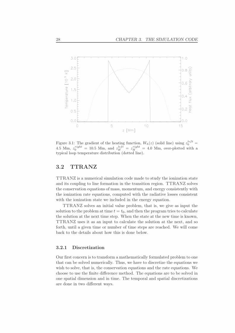
An example of the energy deposition is shown in Figure 3.1. A giventotal energy will produce higher temperatures when deposited in the coronathan in the transition region or chromosphere, since there are fewer particlesto share the energy.
3.1.2 Summary
To solve our problem we need to compute the rate equations, which are de-termined by the conservation equations. We found in the previous sectionthat the energy equation has radiative losses (∂Fr/∂z) as one of its sinkterms. The radiative losses are again determined by the rate equation. Weclearly need a system that solves the conservation equations and the rateequations consistently. This system is a coupled set of non-linear equations,too large to be solved analytically. Therefore, we turn to numerically mod-eling and use the numerical simulation code TTRANZ (Hansteen, 1991).
28 CHAPTER 3. THE SIMULATION CODE
Figure 3.1: The gradient of the heating function, Wh(z) (solid line) using zleft0
=
4.5 Mm, zright0
= 10.5 Mm, and zleftH = zright
H = 4.0 Mm, over-plotted with atypical loop temperature distribution (dotted line).
3.2 TTRANZ
TTRANZ is a numerical simulation code made to study the ionization stateand its coupling to line formation in the transition region. TTRANZ solvesthe conservation equations of mass, momentum, and energy consistently withthe ionization rate equations, computed with the radiative losses consistentwith the ionization state we included in the energy equation.
TTRANZ solves an initial value problem, that is, we give as input thesolution to the problem at time t = t0, and then the program tries to calculatethe solution at the next time step. When the state at the new time is known,TTRANZ uses it as an input to calculate the solution at the next, and soforth, until a given time or number of time steps are reached. We will comeback to the details about how this is done below.
3.2.1 Discretization
Our first concern is to transform a mathematically formulated problem to onethat can be solved numerically. Thus, we have to discretize the equations wewish to solve, that is, the conservation equations and the rate equations. Wechoose to use the finite difference method. The equations are to be solved inone spatial dimension and in time. The temporal and spatial discretizationsare done in two different ways.
3.2. TTRANZ 29
Temporal Discretization
The temporal discretization is done by using a weighted average of theknown, old value (superscript ’o’) and the unknown, new value (super-script ’n’),
y = θy(n) + (1 − θ)y(o), 0 ≤ θ ≤ 1 . (3.7)
We will come back to the details about how the new solution is found inSection 3.2.2. For θ = 1 this is an explicit scheme, for θ 6= 1 this is animplicit scheme, and for θ = 1
2 this method is called the Crank-Nicolsonmethod. We use θ = 0.55.
Spatial Discretization
Even though we are doing our calculations in one dimension, we are stilldividing our space (a line) into boxes, where each box only has two interfaceswhere plasma and heat can flow. The scalars, such as the density and internalenergy, are defined in the center of the boxes, while the vectors, such as thevelocity, are defined at the interfaces.
The spatial discretization is computed using the second order upwindscheme of van Leer (1974). Upwind means that we are choosing which cells toinvolve in the calculation by looking at which direction the advected quantityis moving. For instance, if the velocity is moving to the right we are usingcells to the left of our point to estimate the momentum flux.
A second order method requires information from the two nearest neigh-bor cells on either side of the computational cell being considered. Thisresults in a block penta-diagonal system which needs to be inverted.
The Adaptive Grid
In order to resolve the large gradients and shocks that might arise, the equa-tions are formulated on an adaptive grid. That is, the mesh points are movedtowards the regions where the spatial gradients are large, so that the griddensity is greatest where it at any time is needed the most. The grid stepcan vary in size both as a function of the loop length (z) and time (t).
The grid is allocated to follow gradients in the dynamic variables. Thespatial grid density, ρz = 1/(zi+1 − zi), is computed by solving the gridequation of Dorfi and Drury (1987),
ρz(z) ∝ R(z) ≡
√
1 +
(
zav
fav
df
dz
)2
, (3.8)
where R is the required resolution, f represent any quantity that the gridshould respond to; e.g. u or Te. The subscript ’av’ means that we shoulduse some appropriate average of the subscripted variable, with fav used to

30 CHAPTER 3. THE SIMULATION CODE
weight quantities for which resolution is vital. There is a limit on how far agiven mesh point is allowed to move from one time step to the next.
Allowed changes in grid position as a function of time are controlled ina similar manner.
3.2.2 Calculating the Next Time Step
To go from one (known) time step to the next we have to solve the coupled setof non-linear equations including the grid equation, the conservation equa-tions, and the rate equations for hydrogen and helium. The rate equationsfor the other elements are calculated separately afterwards.
Mathematically the set of equations can be written
Fi(x1, x2, ..., xN ) = 0, i = 1, 2, ..., N , (3.9)
where F is the vector containing the conservation equations and rate equa-tions, while x is the vector containing our variables, z, ρ, n, Te, nHI ...nHmH
,nHeI ...nHemHe
, and ne. Assuming that we have mH levels of hydrogen andmHe levels of helium, this gives 4 + mH + mHe + 1 variables at each depth(grid) point. In total we then have
ndep × (5 + mH + mHe) (3.10)
unknowns to be solved at each time step, where ndep is the number of depthpoints.
Each of the functions in F can be expanded in a Taylor series
Fi(x + δx) = Fi(x) +
N∑
j=i
∂Fi
∂xjδxj + O(δx2) . (3.11)
If Fi is linear in xj then ∂Fi/∂xj is independent of xj and our problemis linear. Hence, the solution for δxj will converge immediately. If Fi isnon-linear, we must iterate to the correct solution at time step ’n’.
Let us denote the current and next iteration step with superscript ’k’and ’k + 1’, respectively, and neglect the terms of order δx2 and higher, sothat
x(k+1) = x
(k) + δx . (3.12)
By introducing vector form and writing the Jacobian ∂Fi
∂xj≡ Jj we get
F(x(k+1)) = F(x(k)) + Jδx = 0 . (3.13)
The correction term can be found by inverting the Jacobian
δx = J−1(−F(x(k))) . (3.14)
3.3. INPUT 31
Since the equations in F are non-linear we can not find the correct solu-tion directly, but if we are sufficiently close to the solution, this methodshould converge. We can now use these new values to recalculate the radi-ative losses, and put them back into the conservation equations for a bettercalculation to be done.
Iterating like this until the correction is less than some preset value iscalled the Newton-Raphson method. The convergence of this method isquadratic, meaning that an error of magnitude ǫ < 1 reduces to ǫ2 in thenext step. This is a very fast convergence, as long as it converges at all. Ifthe initial guess is too far from the solution it never converges, and we haveto restart the calculation of the new time step with a shorter dt. In our casethe convergence usually takes 4-5 iterations.
3.3 Input
We have now discussed how TTRANZ solves our problem, but we have notsaid anything about how we are feeding the program with information. SinceTTRANZ solves an initial value problem, the initial state must be given.In addition, we must inform the program about what our environment lookslike. This is given through the atomic models and the initialization file ’init’.We take a look at these three input sources below.
3.3.1 The Atomic File
Every atom that we want to include in the model must have its one atomicfile, where all the information about the atom is listed. We have included theelements hydrogen, helium, carbon, oxygen, iron, and magnesium. We areinterested in emission lines from helium and iron and therefore, we returnto the details about these elements in Chapter 4. The other elements areincluded because they are among the most abundant elements in the Sun,and therefore these atoms play an important part in the radiative losses attemperatures around 105 K. Thus, it is important to calculate their statescorrectly also when they are driven out of equilibrium.
The atomic model used by TTRANZ is defined by a text file structuredesigned by Carlsson (1986, and later modifications) for the computer pro-gram MULTI. The file is divided into different parts containing the neededinput:
• the element abundances
• the energy levels
• the excitation and de-excitation rates
• the ionization rates
32 CHAPTER 3. THE SIMULATION CODE
We will take a look at the different parts of the file below. Lines markedwith ’∗’ are comments for the reader and are not used by the program. Weuse examples from the iron atomic model
Most of he data in the atomic files are from the HAO-DIAPER package(Judge and Meisner, 1994). We have made some modifications to the ironand helium atomic models, which we discuss in details in Sections 4.2 and4.3.
We use the same set of atomic files throughout the thesis.
Element Abundances
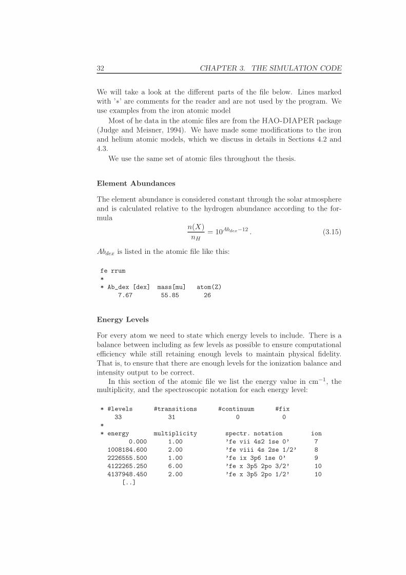
The element abundance is considered constant through the solar atmosphereand is calculated relative to the hydrogen abundance according to the for-mula
n(X)
nH= 10Abdex−12 . (3.15)
Abdex is listed in the atomic file like this:
fe rrum
*
* Ab_dex [dex] mass[mu] atom(Z)
7.67 55.85 26
Energy Levels
For every atom we need to state which energy levels to include. There is abalance between including as few levels as possible to ensure computationalefficiency while still retaining enough levels to maintain physical fidelity.That is, to ensure that there are enough levels for the ionization balance andintensity output to be correct.
In this section of the atomic file we list the energy value in cm−1, themultiplicity, and the spectroscopic notation for each energy level:
* #levels #transitions #continuum #fix
33 31 0 0
*
* energy multiplicity spectr. notation ion
0.000 1.00 ’fe vii 4s2 1se 0’ 7
1008184.600 2.00 ’fe viii 4s 2se 1/2’ 8
2226555.500 1.00 ’fe ix 3p6 1se 0’ 9
4122265.250 6.00 ’fe x 3p5 2po 3/2’ 10
4137948.450 2.00 ’fe x 3p5 2po 1/2’ 10
[..]
3.3. INPUT 33
Excitation and De-excitation Rates
In addition to listing the energy levels we also need to list the possible trans-itions between the different energy levels and what their transition rates are.
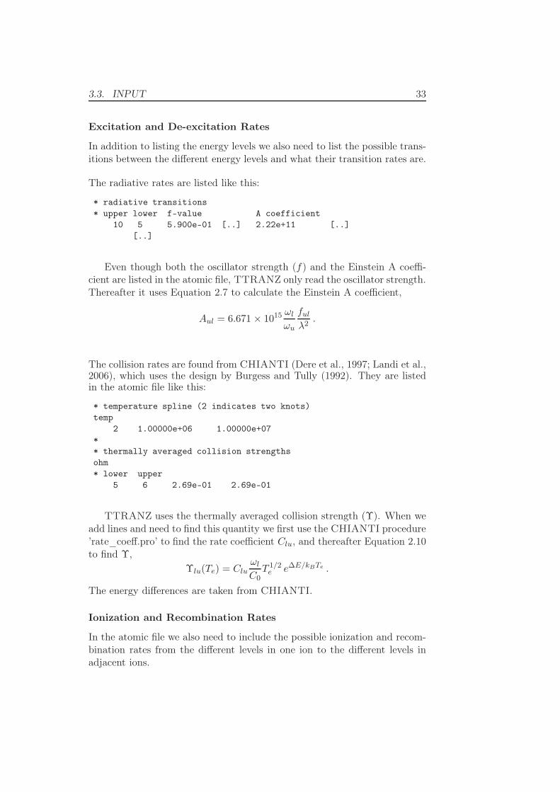
The radiative rates are listed like this:
* radiative transitions
* upper lower f-value A coefficient
10 5 5.900e-01 [..] 2.22e+11 [..]
[..]
Even though both the oscillator strength (f) and the Einstein A coeffi-cient are listed in the atomic file, TTRANZ only read the oscillator strength.Thereafter it uses Equation 2.7 to calculate the Einstein A coefficient,
Aul = 6.671 × 10¹⁵ ωl
ωu
ful
λ2.
The collision rates are found from CHIANTI (Dere et al., 1997; Landi et al.,2006), which uses the design by Burgess and Tully (1992). They are listedin the atomic file like this:
* temperature spline (2 indicates two knots)
temp
2 1.00000e+06 1.00000e+07
*
* thermally averaged collision strengths
ohm
* lower upper
5 6 2.69e-01 2.69e-01
TTRANZ uses the thermally averaged collision strength (Υ). When weadd lines and need to find this quantity we first use the CHIANTI procedure’rate_coeff.pro’ to find the rate coefficient Clu, and thereafter Equation 2.10to find Υ,
Υlu(Te) = Cluωl
C0T 1/2
e e∆E/kBTe .
The energy differences are taken from CHIANTI.
Ionization and Recombination Rates
In the atomic file we also need to include the possible ionization and recom-bination rates from the different levels in one ion to the different levels inadjacent ions.

34 CHAPTER 3. THE SIMULATION CODE
The radiative recombination rates are given by Shull and van Steenberg(1982), and listed in the atom file like this:
shull82
* lower upper acol tcol arad xrad
1 2 0.00e+00 1.45e+06 4.12e-11 7.59e-01
*
* adi bdi t0 t1
2.91e-01 2.29e-01 7.73e+05 6.54e+05
The electron impact ionization rates are given by Arnaud and Raymond(1992), and listed in the atomic file like this:
* electron impact ionization coefficients
ar85-cdi
* lower upper
1 2
* #shell
3
* potential (eV) A B C D
124.20 14.60 -4.36 5.98 -10.50
180.00 67.90 -20.60 9.82 -53.70
220.90 15.60 -2.29 2.30 -10.60
The autoionization rates are given by Arnaud and Raymond (1992), andlisted in the atomic file like this:
ar85-cea
* lower upper
1 2
* Autoionization rate
1.000e+00
The dielectronic recombination rates are given by Burgess (1965), and listedin the atomic file like this:
burgess
* lower upper rate
8 11 1.00e+00
3.3.2 The Init File
Input from the user to the program is given through the init file. In this filewe state what kind of simulation should be done and which considerationsthat should be taken during the program run. The init file must be updatedbefore each simulation, in contrast to the atomic files, which are made onlyonce for one special type of study.
3.3. INPUT 35
The init file is divided into two parts. In the first section we set the timelength of our simulation, how often we save data, and how many iterationswe allow. Here we also specify quantities like the weighting in the tem-poral discretization, the correction limit for the Newton-Raphson method,the maximum allowed change in the grid, which elements to include in thesimulations, and so forth.
In the second part of the init file we decide the length of the loop, wherethe heating is added, and what the heating scale height is. Here we can alsochoose to add waves of different amplitudes to the system. We will addressthe specific input in this part of the init file when discussing our simulationsin Chapter 5.
3.3.3 The Initial Solution
When starting TTRANZ we need the solution to our equations at time t = t0,the initial values. The most common way to solve this challenge is to restartthe program with the output we have from an earlier run. E.g. if we wanta model with a different temperature structure than we already have, wechange the heating function in the init file, start the program and let itsimulate an hour or two (solar time), until the loop has settled. Then wehave the starting point we want for our new simulation.

36 CHAPTER 3. THE SIMULATION CODE
Chapter 4
The Atomic Model
In this chapter we describe our atomic models. Recall from Section 3.3.1 thatevery atom included in our model must be defined in an atomic file, whereall the energy levels, transitions, and rates are listed. We limit ourselvesto go through in detail the atoms which have interesting lines in the EISwavelength band.
Before designing our atoms, we first have to look at the possibilities andlimitations of the spectrograph we are analyzing. We identify the spectrallines usable for our purpose and plot the contribution functions for the mostinteresting ones. Thereafter, we look in details at the atoms we choose touse lines from, that is iron and helium. We identify which energy levels andlines to include and check that our ionization balances are correct.
4.1 Identifying Spectral Lines
We want to simulate detections from the extreme ultraviolet (EUV) ima-ging spectrograph (EIS) on board Hinode (Solar-B). EIS can observe in twowavelength intervals, 170–210 Å (the short wavelength band) and 250–290 Å(the long wavelength band). It is expected to have a spectral resolution of3 km/s for Doppler velocities (Culhane et al., 2007). Some EIS specifica-tions are listed in Table 4.1. We have to consider these specifications whenchoosing which spectral lines to examine.
Wavelength coverage 170–210 Å and 250–290 ÅDispersion 0.0223 Å/CCD pixelPixel equivalent width 34.3 km/s for 195 Å, and 23.6 km/s for 284 Å
Table 4.1: EIS specifications.
37
38 CHAPTER 4. THE ATOMIC MODEL
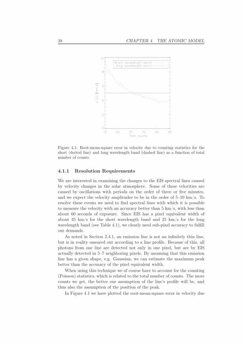
Figure 4.1: Root-mean-square error in velocity due to counting statistics for theshort (dotted line) and long wavelength band (dashed line) as a function of totalnumber of counts.
4.1.1 Resolution Requirements
We are interested in examining the changes to the EIS spectral lines causedby velocity changes in the solar atmosphere. Some of these velocities arecaused by oscillations with periods on the order of three or five minutes,and we expect the velocity amplitudes to be in the order of 5–10 km/s. Toresolve these events we need to find spectral lines with which it is possibleto measure the velocity with an accuracy better than 5 km/s, with less thanabout 60 seconds of exposure. Since EIS has a pixel equivalent width ofabout 35 km/s for the short wavelength band and 25 km/s for the longwavelength band (see Table 4.1), we clearly need sub-pixel accuracy to fulfillour demands.
As noted in Section 2.4.1, an emission line is not an infinitely thin line,but is in reality smeared out according to a line profile. Because of this, allphotons from one line are detected not only in one pixel, but are by EISactually detected in 5–7 neighboring pixels. By assuming that this emissionline has a given shape, e.g. Gaussian, we can estimate the maximum peakbetter than the accuracy of the pixel equivalent width.
When using this technique we of course have to account for the counting(Poisson) statistics, which is related to the total number of counts. The morecounts we get, the better our assumption of the line’s profile will be, andthus also the assumption of the position of the peak.
In Figure 4.1 we have plotted the root-mean-square error in velocity due
4.1. IDENTIFYING SPECTRAL LINES 39
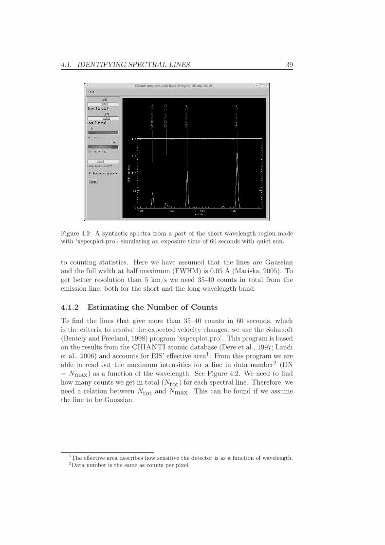
Figure 4.2: A synthetic spectra from a part of the short wavelength region madewith ’xspecplot.pro’, simulating an exposure time of 60 seconds with quiet sun.
to counting statistics. Here we have assumed that the lines are Gaussianand the full width at half maximum (FWHM) is 0.05 Å (Mariska, 2005). Toget better resolution than 5 km/s we need 35-40 counts in total from theemission line, both for the short and the long wavelength band.
4.1.2 Estimating the Number of Counts
To find the lines that give more than 35–40 counts in 60 seconds, whichis the criteria to resolve the expected velocity changes, we use the Solarsoft(Bentely and Freeland, 1998) program ’xspecplot.pro’. This program is basedon the results from the CHIANTI atomic database (Dere et al., 1997; Landiet al., 2006) and accounts for EIS’ effective area1. From this program we areable to read out the maximum intensities for a line in data number2 (DN= Nmax) as a function of the wavelength. See Figure 4.2. We need to findhow many counts we get in total (Ntot) for each spectral line. Therefore, weneed a relation between Ntot and Nmax. This can be found if we assumethe line to be Gaussian.
1The effective area describes how sensitive the detector is as a function of wavelength.2Data number is the same as counts per pixel.
40 CHAPTER 4. THE ATOMIC MODEL
Relation Between Nmax and Ntot for a Gaussian
The equation for a Gaussian distribution G(x) with area Ntot (which canbe associated by the total number of counts from one line) and standarddeviation σ is given by
G(x) =Ntotσ√
2πe−
(
x2
2σ2
)
. (4.1)
The relation between Nmax and Ntot is given by
G(0) = Nmax =Ntotσ√
2π
⇓Ntot = Nmax · σ
√2π .
(4.2)
The half maximum is found when e−
(
x2
2σ2
)
= 12 , that is x = σ
√2 ln 2. FWHM
is twice this size, and thus given by
FWHM = 2σ√
2 ln 2 . (4.3)
This leads to the standard deviation
σ =FWHM
2√
2 ln 2. (4.4)
Putting this into Equation 4.2 gives
Ntot = Nmax · FWHM ·√
π
2√
ln 2
≈ Nmax · FWHM .
(4.5)
If we assume that we need a total of at least 40 counts from each line,this relates to DN as
DN = Nmax =Ntot
FWHM=
40 counts0.05Å
0.0223Å/pix
≈ 18 counts/pix , (4.6)
where we have converted the FWHM of 0.05 Å into pixels by dividing bythe dispersion, 0.0223/pix (see Table 4.1). To be able to resolve the velocitybetter than 5 km/s, we must thus have a spectral line with maximum countsper pixel greater than 18.
4.1. IDENTIFYING SPECTRAL LINES 41
Wavelength Ion Temp. DN Lower level Upper level[Å] [lg(T )] [counts/pix]
Short band184.5 Fe X 6.0 18 3p5 2P3/2 3p4 (1D) 3d 2S1/2
186.9 Fe XII 6.1 21 3p3 2D5/2 3p2 (3P) 3d 2F7/2
188.2 Fe XI 6.1 65 3p4 3P2 3p3 (2D) 3d 3P2
192.4 Fe XII 6.1 77 3p3 4S3/2 3p2 (3P) 3d 4P1/2
192.8 Fe XI 6.1 26 3p4 3P1 3p3 (2D) 3d 3P2
193.5 Fe XII 6.1 182 3p3 4S3/2 3p2 (3P) 3d 4P3/2
195.1 Fe XII 6.1 285 3p3 4S3/2 3p2 (3P) 3d 4P5/2
198.6 S VIII 5.9 27 2p5 2P3/2 2s 2p6 2S1/2
202.0 Fe XIII 6.2 72 3p2 3P0 3p 3d 3P1
203.2 Fe XIII 6.2 2 3p2 3P1 3p 3d 3P0
203.8 Fe XIII 6.3 16 3p2 3P2 3p 3d 3D3
Long band256.3 He II 4.9 22 1s 2S1/2 3p 2P3/2 (P1/2)274,2 Fe XIV 6.3 20 3p 2P1/2 3s 3p2 2S1/2
284,2 Fe XV 6.3 30 3s2 1S0 3s 3p 1P1
Table 4.2: Wavelength, temperature of peak abundance, spectral notation, andcounts per pixel (assuming quiet sun) for the chosen EIS spectral lines. Full shellsare not included in the spectral notation.
4.1.3 Selected Lines
From ’xspecplot.pro’ we find the spectral lines which have Nmax higher than18 for quiet sun with an exposure time of 60 seconds. Their wavelengths,temperatures of peak abundance, spectral notations, and data numbers arelisted in Table 4.2. To this list we have also added the Fe XIII lines 203.2 Åand 203.8 Å, which can be used for density diagnostics in combination withthe Fe XIII 202.0 Å line. He II 256.317 Å and 256.318 Å are for simplicitytreated as only one line, He II 256.3 Å. This line is blended by Si X 256.4 Å.
The list include interesting lines from the atoms iron, helium, and sulfur.We have not included the element sulfur in our atomic model, but we willgo through the two other elements in greater details below.
The Contribution Functions
As stated in Section 2.4.3, the contribution function gives information aboutwhich temperature interval an emission line is formed at. The temperaturenoted in Table 4.2 is the temperature where the contribution function hasthe greatest value. To get a better understanding about where the lines areformed we have plotted the contribution functions for our iron lines in Figure
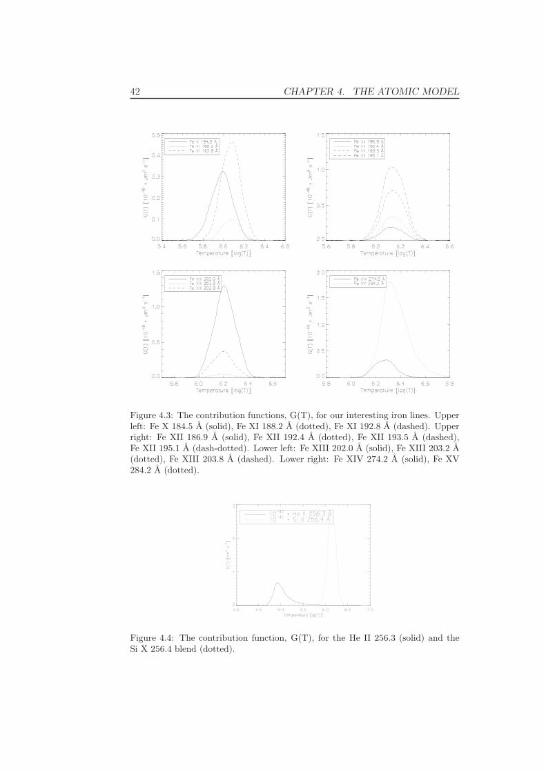
42 CHAPTER 4. THE ATOMIC MODEL
Figure 4.3: The contribution functions, G(T), for our interesting iron lines. Upperleft: Fe X 184.5 Å (solid), Fe XI 188.2 Å (dotted), Fe XI 192.8 Å (dashed). Upperright: Fe XII 186.9 Å (solid), Fe XII 192.4 Å (dotted), Fe XII 193.5 Å (dashed),Fe XII 195.1 Å (dash-dotted). Lower left: Fe XIII 202.0 Å (solid), Fe XIII 203.2 Å(dotted), Fe XIII 203.8 Å (dashed). Lower right: Fe XIV 274.2 Å (solid), Fe XV284.2 Å (dotted).
Figure 4.4: The contribution function, G(T), for the He II 256.3 (solid) and theSi X 256.4 blend (dotted).

4.2. DESIGNING THE IRON MODEL 43
4.3, and the helium line with the silicon blend in Figure 4.4.3 Note that thehelium and silicone lines are formed in two different temperature intervals,and that the silicone line’s contribution function takes on much higher valuesthan the helium one.
4.2 Designing the Iron Model
When we do numerical simulations it is important to decide to what degreewe want to include physical details in the simulations. The more detailswe include, the more computationally demanding the simulations become.It is important to find the balance between computational complexity andaccuracy. Because of this we have to pay attention to the information weinclude in the atomic model. In the following subsections we will go throughthe different iron ions and explain which levels we have chosen to include inour model.
To make our iron-model we use the HAO-DIAPER package (Judge andMeisner, 1994) as a starting point. Where this model lacks information weuse the CHIANTI atomic database (Dere et al., 1997; Landi et al., 2006)to find the wavelength and spectral configuration, and the NIST onlinedatabase (Ralchenko et al., 2005) to find the oscillator strength. We willcome back to details about this below.
4.2.1 Included Ions
As can be seen from Table 4.2 we are interested in lines from the ions Fe X –Fe XV. If we include only these ions, the ionization balance would not becorrect, because there exist other iron ions in the same temperature interval.Therefore, we must include extra iron ions, even if we are not interested intheir lines. We choose to include the ions Fe VII – Fe XVIII in our model.Ions outside this interval will only marginally influence our results. We willcome back to the ionization balance in Section 4.2.4.
4.2.2 Included Energy Levels
Now we have chosen which ions to include, and it is time to consider whichenergy levels to include for each of them. The de-excitation rates for most ofthe excited levels are much higher than the rates at which they are excited.Therefore, there are very few ions in the excited stages. As noted in Section2.2.3, this is not the case for meta-stable levels. We include the ground level,which of course is the state in which most of the ions are, and the upper andlower levels of our lines. In addition, we must consider whether there are
3These figures are made with the CHIANTI procedure ’ch_synthetic’ with data fromMazzotta et al. (1998).

44 CHAPTER 4. THE ATOMIC MODEL
any low-lying meta-stable levels which a notable fraction of the ions mightbe in. If so, these must be included too.
Ions Without Interesting Lines
We are not interested in lines from the ions Fe VII – Fe IX and Fe XVI –Fe XVIII. These are included only for the ionization balance to be correct. Itdoes not matter for us whether the ions are in the ground or excited states,since this does not affect the ionization balance notably. Therefore, we onlyinclude the ground levels of these ions.
Ions With Interesting Lines
For the ions Fe X – Fe XV we are interested in the lines listed i Table4.2. In addition to the levels listed in this table, we use the CHIANTI
procedure ’show_pops.pro’ to examine if there are any meta-stable levelsthat a notable part of the ions are in. We choose only to include levels withpopulation higher than 5% of the total ion population. We go through theresults below. The levels we include are summarized in Table 4.3, and theGrotrian diagrams4 for the different ions can be seen if Figure 4.5.
Fe X has only one line we are interested in, 184.5 Å. We include the lowerand upper level of this line, 3p5 2P3/2 and 3p4 (1D) 3d 2S1/2. The firstis also the ground level of the ion. In addition this ion has one meta-stable level which has a substantial fraction of the ion’s population(19%), 3p5 2P3/2, which we include. Fe X is plotted in the upper leftpanel of Figure 4.5.
Fe XI has two lines we are interested in, 188.2 Å and 192.8 Å. The first linehas the ground level as its lower level, 3p4 3P2, while the second linehas a meta-stable level as its lower level, 3p4 3P1. The lines have acommon upper level, 3p3 (2D) 3d 3P2. In addition to these levels, wealso include two meta-stable levels, 3p4 3P0 which has 6% of the ion’spopulation and 3p4 1D2 which has 12%. Fe XI is plotted in the upperright panel of Figure 4.5.
Fe XII has four lines we are interested in, 186.9 Å, 192.4 Å, 193.5 Å,and 195.1 Å. The first line has 3p3 2D5/2 as its lower level while thethree others have 3p3 4S3/2. Their upper levels are 3p2 (3P) 3d 2F7/2,3p2 (3P) 3d 4P1/2, 3p2 (3P) 3d 4P3/2, and 3p2 (3P) 3d 4P5/2, respect-ively. In addition to these levels we also include the ground level, 3p3
2D3/2. Fe XII is plotted in the middle left panel of Figure 4.5.
4The Grotrian diagrams are made with the HAO-DIAPER procedure ’termdiag.pro’.
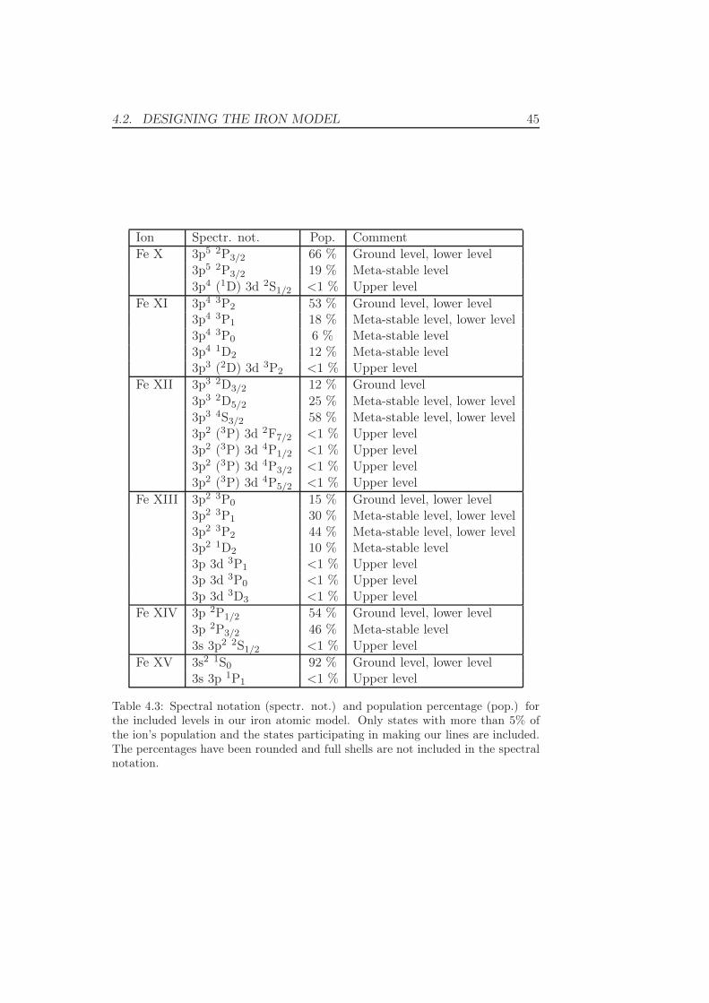
4.2. DESIGNING THE IRON MODEL 45
Ion Spectr. not. Pop. CommentFe X 3p5 2P3/2 66 % Ground level, lower level
3p5 2P3/2 19 % Meta-stable level3p4 (1D) 3d 2S1/2 <1 % Upper level
Fe XI 3p4 3P2 53 % Ground level, lower level3p4 3P1 18 % Meta-stable level, lower level3p4 3P0 6 % Meta-stable level3p4 1D2 12 % Meta-stable level3p3 (2D) 3d 3P2 <1 % Upper level
Fe XII 3p3 2D3/2 12 % Ground level3p3 2D5/2 25 % Meta-stable level, lower level3p3 4S3/2 58 % Meta-stable level, lower level3p2 (3P) 3d 2F7/2 <1 % Upper level3p2 (3P) 3d 4P1/2 <1 % Upper level3p2 (3P) 3d 4P3/2 <1 % Upper level3p2 (3P) 3d 4P5/2 <1 % Upper level
Fe XIII 3p2 3P0 15 % Ground level, lower level3p2 3P1 30 % Meta-stable level, lower level3p2 3P2 44 % Meta-stable level, lower level3p2 1D2 10 % Meta-stable level3p 3d 3P1 <1 % Upper level3p 3d 3P0 <1 % Upper level3p 3d 3D3 <1 % Upper level
Fe XIV 3p 2P1/2 54 % Ground level, lower level3p 2P3/2 46 % Meta-stable level3s 3p2 2S1/2 <1 % Upper level
Fe XV 3s2 1S0 92 % Ground level, lower level3s 3p 1P1 <1 % Upper level
Table 4.3: Spectral notation (spectr. not.) and population percentage (pop.) forthe included levels in our iron atomic model. Only states with more than 5% ofthe ion’s population and the states participating in making our lines are included.The percentages have been rounded and full shells are not included in the spectralnotation.
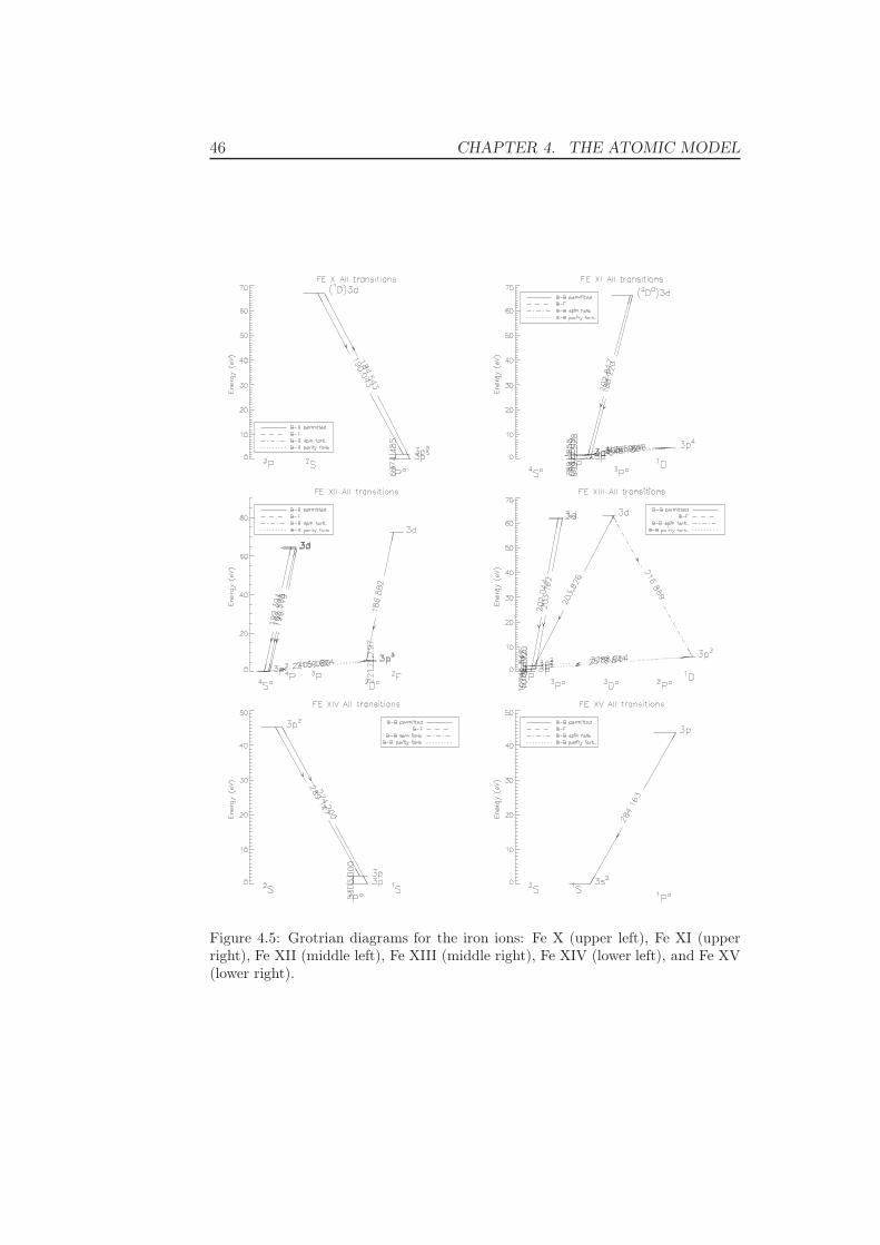
46 CHAPTER 4. THE ATOMIC MODEL
Figure 4.5: Grotrian diagrams for the iron ions: Fe X (upper left), Fe XI (upperright), Fe XII (middle left), Fe XIII (middle right), Fe XIV (lower left), and Fe XV(lower right).

4.2. DESIGNING THE IRON MODEL 47
Fe XIII has three interesting lines, 202.0 Å, 203.2 å and 203.8 Å. The firstline has the ground level as its lower level, 3p2 3P0, while the othershave two meta-stable levels as their lower levels, 3p2 3P1 and 3p2 3P2.Their upper levels are 3p 3d 3P1, 3p 3d 3P0, and 3p 3d 3D3, respect-ively. In addition, we include a meta-stable level, 3p2 1D2, which has10% of the ion’s population. Fe XIII is plotted in the middle rightpanel of Figure 4.5.
Fe XIV has only one line we are interested in, 274.2 Å. This line has theground level as its lower level, 3p 2P1/2, and 3s 3p2 2S1/2 as its upperlevel. In addition to these levels we include the meta-stable level, 3p2P3/2, which has 46% of the ion’s population. Fe XIV is plotted in thelower left panel of Figure 4.5.
Fe XV has only one line we are interested in, 284.2 Å. This line has theground level as its lower level, 3s2 1S0, and 3s 3p 1P1 as its upper level.This ion has no meta-stable levels in which a substantial fraction ofthese ions are in. Fe XV is plotted in the lower right panel of Figure4.5.
4.2.3 Particular Changes
Two of the ions in the HAO-DIAPER package, Fe XIII and Fe XV, do notinclude the levels and lines we are interested in. We therefore take a look atthe changes we have made to them below.
FE XIII
The 202.0 Å line is not included in the DIAPER file, but both the upperand lower levels are. We add this line with the oscillation strength fromAggarwal and Keenan (2004) and the collision strengths from CHIANTI.
The 203.2 Å line is listed with the wrong wavelength and further exam-inations show that the upper level is listed with wrong energy compared toCHIANTI. This is therefore changed from 503340 cm−1 to 501520 cm−1.
FE XV
The 284.2 Å line is not included in the DIAPER file. When comparing thespectral notation with levels and lines in CHIANTI and NIST we find thatthe upper level is listed with wrong energy value and therefore the wavelengthis wrong. We change the energy from 355439.156 cm−1 to 351911.000 cm−1,and keep the rest of the parameters unchanged.
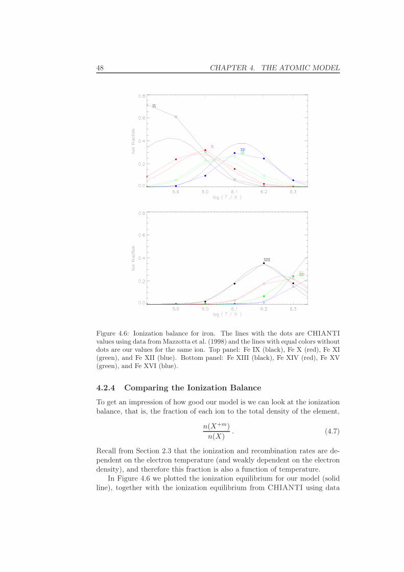
48 CHAPTER 4. THE ATOMIC MODEL
Figure 4.6: Ionization balance for iron. The lines with the dots are CHIANTI
values using data from Mazzotta et al. (1998) and the lines with equal colors withoutdots are our values for the same ion. Top panel: Fe IX (black), Fe X (red), Fe XI(green), and Fe XII (blue). Bottom panel: Fe XIII (black), Fe XIV (red), Fe XV(green), and Fe XVI (blue).
4.2.4 Comparing the Ionization Balance
To get an impression of how good our model is we can look at the ionizationbalance, that is, the fraction of each ion to the total density of the element,
n(X+m)
n(X). (4.7)
Recall from Section 2.3 that the ionization and recombination rates are de-pendent on the electron temperature (and weakly dependent on the electrondensity), and therefore this fraction is also a function of temperature.
In Figure 4.6 we plotted the ionization equilibrium for our model (solidline), together with the ionization equilibrium from CHIANTI using data
4.3. DESIGNING THE HELIUM MODEL 49
from Mazzotta et al. (1998) (dotted line). The ions have the same color forboth models. Note that there are much fever data points in the CHIANTI
data, which makes the comparison more difficult.Our Fe IX and Fe XVI ionic data do not agree with the CHIANTI data;
the former gives a much lower ionization fraction, while the latter gives amuch higher fraction. This disagreement is acceptable since we have no linesfrom these ions. On the other hand, the ions we are interested in, Fe X –Fe XV agree quite well with the CHIANTI data. Fe X, Fe XI and Fe XIIshow a bit too low ionization fraction at temperatures lower than 106 K, butare elsewhere in good agreement, assuming the CHIANTI data are missingthe point of maximum fraction for the Fe XII ion. Fe XIII, Fe XIV andFe XV are in good agreement, assuming the CHIANTI data are missing thepoint of maximum fraction for the Fe XIV and Fe XV ions.
4.3 Designing the Helium Model
Helium is the other atom we want to design to be able to examine the Hinodelines. The only helium line we are interested in is the He II 256.3 Å line.This is in reality two lines (256.317 Å and 256.318 Å), but the wavelengthdifference is so small that we consider them as only one line. This line isblended by the Si 256.4 Å line.
4.3.1 Included Ions and Levels
Helium has only three possible ionization stages, so for the ionization balanceto be as correct as possible we include all of them.
Our atom file was originally made to study the 10840 Å line and includesnine energy levels. This file is made with the HAO-DIAPER package anduses excitation and ionization rates from Arnaud and Rothenflug (1985);Shull and van Steenberg (1982); Burgess (1965), and photoionization ratesfrom Avrett et al. (1976). Instead of spending a lot of time examining whichlevels could be removed, we choose to keep these nine levels and only addthe extra energy level and the transition rates for our line.
The information about the energy levels and rates for the combined 256.3line are found from the HAO-DIAPER package. A Grotrian diagram5 forour helium atom can be seen in Figure 4.7.
4.3.2 Comparing the Ionization Balance
As for hydrogen, we want to examine how good our model is. In Figure4.8 we have plotted the ionization equilibria for our helium model (solidline) along with the ionization equilibrium from CHIANTI using data from
5The Grotrian diagrams are made with the HAO-DIAPER procedure ’termdiag.pro’.

50 CHAPTER 4. THE ATOMIC MODEL
Figure 4.7: Grotrian diagram for the helium atom.
Figure 4.8: Ion balance for helium. He I (black), He II (red), and He III (green).The lines with the dots are CHIANTI values using data from Mazzotta et al. (1998)and the lines with equal colors without dots are our values for the same ion.

4.3. DESIGNING THE HELIUM MODEL 51
Mazzotta et al. (1998) (dotted line). As can be seen, the fit is generallyquite good. At T = 104.9 K and warmer, where our helium line is formed,the fit is very good. Note that here it is our data which has less data points.This is because the adaptive grid allocates the grid points away from thealmost isothermal chromosphere and towards the transition region wherethe temperature and density gradients are larger.

52 CHAPTER 4. THE ATOMIC MODEL
Chapter 5
Simulations
In this chapter we perform numerical simulations using the simulation codeTTRANZ and our atomic model. First we give an introduction to our loopmodel and a short repetition of the heating mechanisms. Then we run threedistinct experiments: an initially hot loop that cools, an initially cold loopthat is rapidly heated, and a loop buffeted by acoustic waves from below.For each simulation we go through the morphological changes in the loop.Thereafter, we study how the different EIS spectral lines react to the event,and examine whether any of our lines are driven out of ionization equilibrium.Finally, we discuss which changes EIS is actually able to detect and whetherthese changes can give us information about the physical processes in thesolar atmosphere.
5.1 The Loop Model
Loop Geometry and Boundary Conditions
The topology of the magnetic field in the solar atmosphere consists of loopswith footpoints connecting different photospheric regions. When the mag-netic field is strong (low β) the dynamics in the plasma are constrained tofollow the magnetic field lines. Our loop model tries to resemble the plasmain one loop. z is defined as a 180◦ semi-circular flux tube of length 15 Mmand with no inclination relative to the vertical. The loop has footpoints inthe middle chromosphere, stretching through the transition region and upinto the almost isothermal corona. The area of the flux tube is kept constant,which should be acceptable for a low β coronal loop.
The footpoint boundaries are set up so that the temperature and pressureare driven towards 7000 K and 100 Pa, respectively, while at the same timevarying in a manner that allows the propagation of sound waves out of thecomputational domain without reflection.
53
54 CHAPTER 5. SIMULATIONS
The Heating Mechanism
As described in Section 2.5 the internal energy, and thus the temperature,are defined by the conservation of energy equation (Equation 2.57),
∂
∂t(ρe) +
∂
∂z(ρue) + (p + Q)
∂u
∂z=
∂
∂z(Fc + Fr + Fh) .
Radiative losses (∂Fr/∂z) are determined by radiation mainly in the spec-tral lines of highly ionized elements such as carbon, oxygen, and iron, and inpart by radiative recombination, and at temperatures higher than 1 MK, bybremsstrahlung. The conductive flux (Fc) is determined solely by the tem-perature profile, while the amplitude and scale height of the heating function(Fh) are set manually in the ’init’ file (cf. Section 3.3.2). It is therefore thelatter parameter we can adjust to make changes in the temperature distribu-tion of our atmosphere. All our simulations are run with a heating functionthat exponentially decays with a scale height of 4 Mm, while the heatingamplitude is varied according to the experiment being conducted. Equalamounts of energy are inserted into both footpoints. The sources and sinksin the energy equation are described in greater detail in Section 3.1.1.
In this work we are not interested in the nature of the heating, only thedynamic effects it has on the emission lines’ intensities and Doppler shiftsas detected by the EIS instrument. Our aims are to present a physicallyreasonable scenario and to pursue its consequences in the EIS spectral lines.
Before starting our simulations we let the system relax into a steadystate, which is reached when the three sources and sinks are in balance,
∂
∂z(Fc + Fr + Fh) = 0 . (5.1)
This is done to ensure that we are starting from an atmospheric state thatis more or less in equilibrium, so that we can isolate the effects we arespecifically studying here.
5.2 Warm Loop Cooling
An initially warm loop has been constructed and is shown in Figure 5.1. Inthe left panel we plot the logarithm of the temperature, pressure and electrondensity as functions of position along the loop (z). In the right panel we plotthe plasma velocity as a function of z.
The temperature is of order 6000 K in the loop footpoints (z = 0 Mm andz = 15 Mm) extending almost 1 Mm up before the rapid transition regiontemperature rise is encountered. Here at z ∼ 0.6 Mm the temperature risesto some 1.8 MK in a few Mm. This temperature structure is maintained byan input heat flux of 6000 W/m2 in both sides of the loop, deposited fromzleft0 = 4.5 Mm and zright
0 = 10.5 Mm, with a scale height zleftH = zright
H =

5.2. WARM LOOP COOLING 55
Figure 5.1: Left panel: The initial distribution of temperature (solid), pressure(dashed) and electron density (dotted) with distance (z) along loop. Right panel:The initial velocity distribution with distance (z) along loop.
4.0 Mm. See Figure 3.1. The electron density starts out at 3×10¹⁸ m−3 in thefootpoints, decreasing to 2×10¹⁷ m−3 in the upper part of the chromosphere.In the transition region the density drops of even more, and continues todecrease down to 1016 m−3 in the corona.
The pressure starts of at 100 Pa in the footpoints, decreasing rapidlywith a scale height1 of some 100 km in the chromosphere, to about 0.5 Pa atthe bottom of the transition region. As the temperature rises the pressurescale height increases and the pressure is almost constant through the upperpart of the loop. As seen in the right panel of Figure 5.1, the velocity isnearly zero through the entire initial model.
At time t = 0 s the heating amplitude is reduced to 60 W/m2, and keptat that value throughout the simulation. No other changes are made.
5.2.1 Loop Changes
We will describe the morphology of the loop plasma in terms of the thermo-dynamical variables temperature, velocity, and density, and describe thechanges caused by the abrupt reduction in heat deposition. Have in mindthat these are actually changes in the loop morphology, and not necessarily
1The pressure scale height is given by Hp =kBT
mg, where g =
GMr
r2 is the local acceler-ation of gravity.
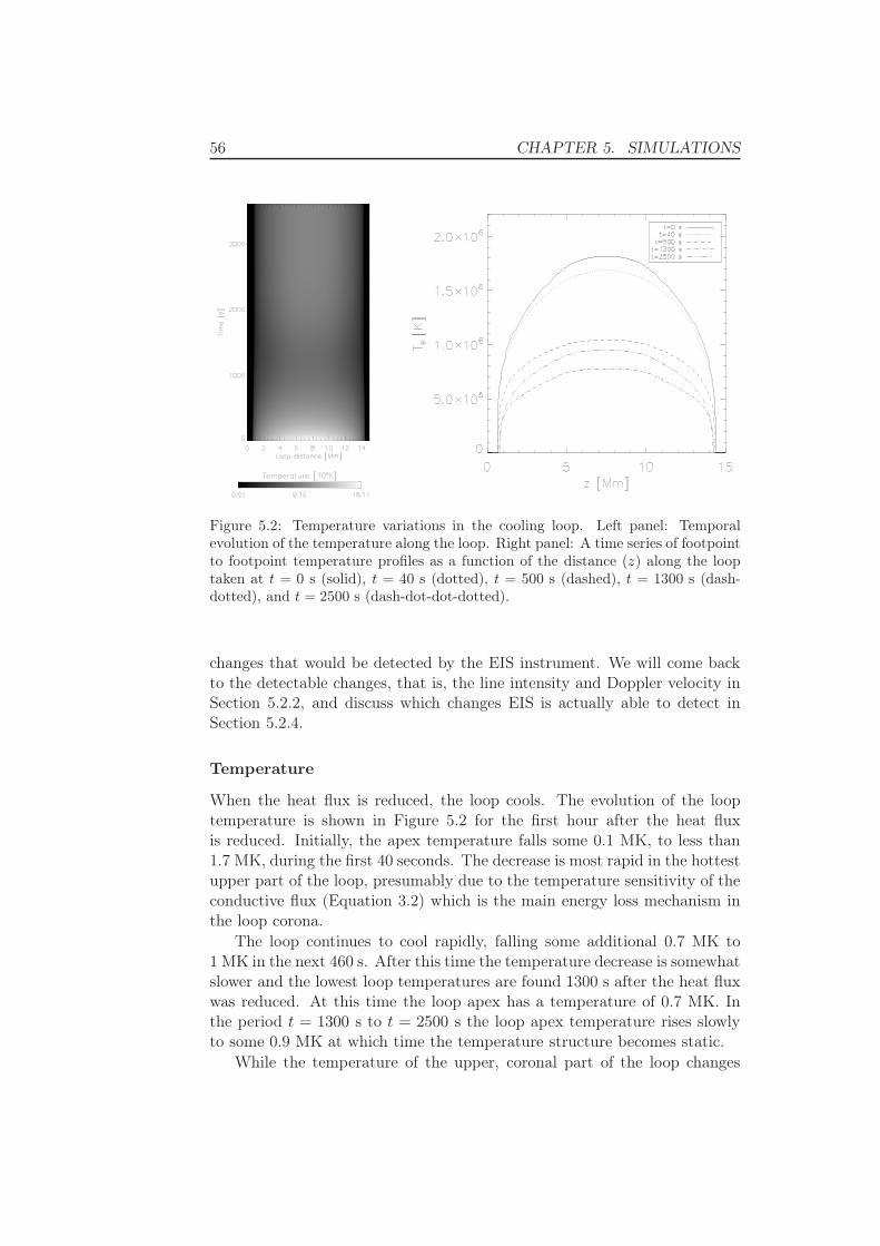
56 CHAPTER 5. SIMULATIONS
Figure 5.2: Temperature variations in the cooling loop. Left panel: Temporalevolution of the temperature along the loop. Right panel: A time series of footpointto footpoint temperature profiles as a function of the distance (z) along the looptaken at t = 0 s (solid), t = 40 s (dotted), t = 500 s (dashed), t = 1300 s (dash-dotted), and t = 2500 s (dash-dot-dot-dotted).
changes that would be detected by the EIS instrument. We will come backto the detectable changes, that is, the line intensity and Doppler velocity inSection 5.2.2, and discuss which changes EIS is actually able to detect inSection 5.2.4.
Temperature
When the heat flux is reduced, the loop cools. The evolution of the looptemperature is shown in Figure 5.2 for the first hour after the heat fluxis reduced. Initially, the apex temperature falls some 0.1 MK, to less than1.7 MK, during the first 40 seconds. The decrease is most rapid in the hottestupper part of the loop, presumably due to the temperature sensitivity of theconductive flux (Equation 3.2) which is the main energy loss mechanism inthe loop corona.
The loop continues to cool rapidly, falling some additional 0.7 MK to1 MK in the next 460 s. After this time the temperature decrease is somewhatslower and the lowest loop temperatures are found 1300 s after the heat fluxwas reduced. At this time the loop apex has a temperature of 0.7 MK. Inthe period t = 1300 s to t = 2500 s the loop apex temperature rises slowlyto some 0.9 MK at which time the temperature structure becomes static.
While the temperature of the upper, coronal part of the loop changes
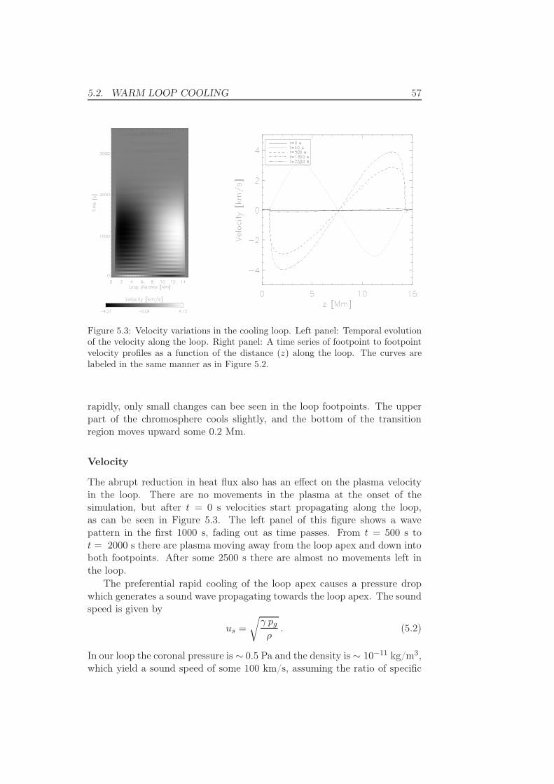
5.2. WARM LOOP COOLING 57
Figure 5.3: Velocity variations in the cooling loop. Left panel: Temporal evolutionof the velocity along the loop. Right panel: A time series of footpoint to footpointvelocity profiles as a function of the distance (z) along the loop. The curves arelabeled in the same manner as in Figure 5.2.
rapidly, only small changes can bee seen in the loop footpoints. The upperpart of the chromosphere cools slightly, and the bottom of the transitionregion moves upward some 0.2 Mm.
Velocity
The abrupt reduction in heat flux also has an effect on the plasma velocityin the loop. There are no movements in the plasma at the onset of thesimulation, but after t = 0 s velocities start propagating along the loop,as can be seen in Figure 5.3. The left panel of this figure shows a wavepattern in the first 1000 s, fading out as time passes. From t = 500 s tot = 2000 s there are plasma moving away from the loop apex and down intoboth footpoints. After some 2500 s there are almost no movements left inthe loop.
The preferential rapid cooling of the loop apex causes a pressure dropwhich generates a sound wave propagating towards the loop apex. The soundspeed is given by
us =
√
γ pg
ρ. (5.2)
In our loop the coronal pressure is ∼ 0.5 Pa and the density is ∼ 10−11 kg/m3,which yield a sound speed of some 100 km/s, assuming the ratio of specific

58 CHAPTER 5. SIMULATIONS
heats to be γ = 5/3. From the left panel of Figure 5.3 the sound waveperiod is estimated to be 100 s, giving a wavelength of some 10 Mm. Thiswavelength is much larger than the temperature scale height in the transitionregion and the wave is reflected due the rapid change in sound speed. Thus,the wave is trapped in the corona, and is bouncing back and forth betweenthe two footpoints. It is this standing wave which is visible in the left panelof Figure 5.3 during the first 1000 s of our simulation. The amplitude ofthe wave is initially some 3 km/s, which can be seen at t = 40 s (dottedline) in the right panel of the figure. The velocity drops steadily as thewave is damped, presumably due to leakage into the transition region or byradiative damping. The amplitudes in the lower parts of the loop decreasefastest because of the higher density.
The changes in temperature described above have consequences for thepressure balance in the loop. The loop is being supported by the pressuregradient, and when the temperature changes, so does the pressure, accordingto Equation 2.55,
p =ρkBT
m.
As the plasma cools it loses hydrostatic support, causing the material todrain out of the loop. First, as noted above, the temperature and thus thepressure near the top of the loop falls very rapidly, causing a short lived up-flow towards the loop apex. As the loop continues to cool, the flow is beingmoved downwards with an increasing velocity, reaching a 4 km/s maximumsome 1300 s after the simulation begins. As the loop re-heats, the flow slowsand the velocity is nearly zero after 2500 s.
Density
As seen in Figure 5.4 the density is almost unchanged during the first500 s after the onset of our simulation. However, after this time and un-til t = 1300 s the density at the loop apex is reduced by a factor three asmaterial drains out of the loop, from log(ρ) = −10.8 to log(ρ) = −11.2.After this time the density continues to decrease, though more slowly, andfirst stabilizes after 2500 s at log(ρ) = −11.4. While the fall of density inthe corona is dramatic, only small changes are seen in the density structureof the transition region and none is seen in the chromosphere.
The measured drop in density can explain the temperature increase inthe latter stages of our simulation after t = 1300 s. The energy input isconstant throughout the simulation, and a reduction in density causes fewerparticles to share this energy input. As a result the temperature will riseslightly as the density drops.
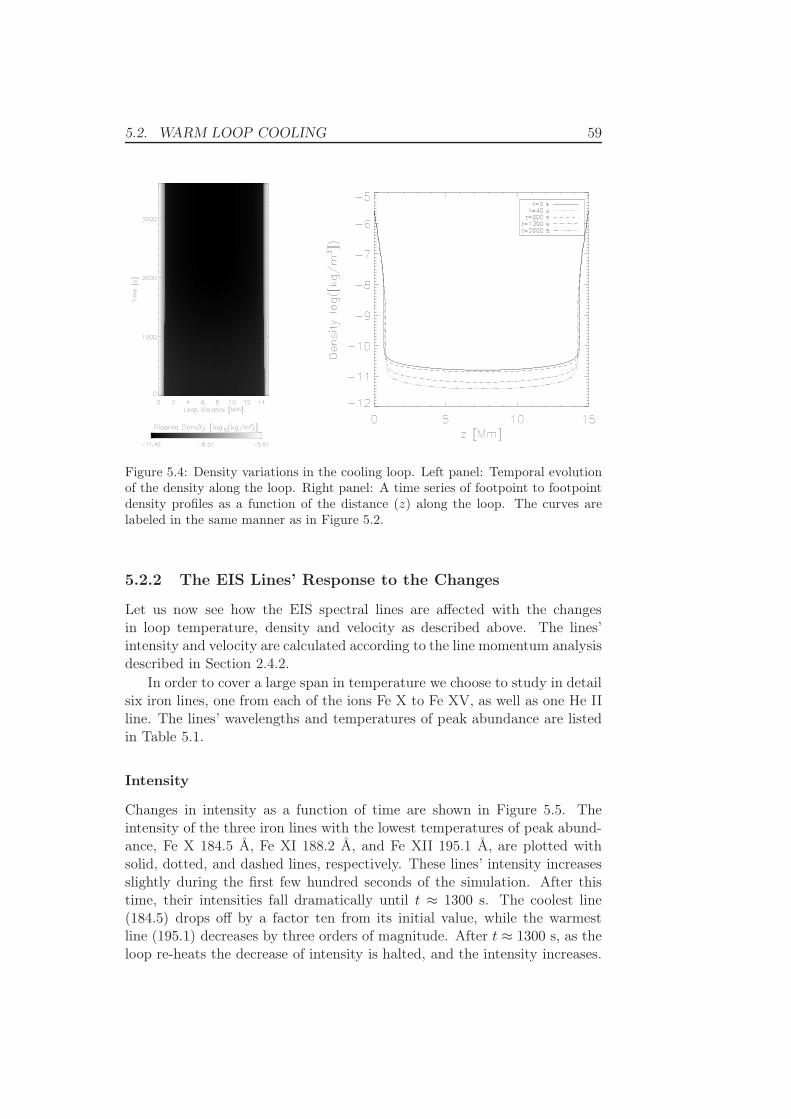
5.2. WARM LOOP COOLING 59
Figure 5.4: Density variations in the cooling loop. Left panel: Temporal evolutionof the density along the loop. Right panel: A time series of footpoint to footpointdensity profiles as a function of the distance (z) along the loop. The curves arelabeled in the same manner as in Figure 5.2.
5.2.2 The EIS Lines’ Response to the Changes
Let us now see how the EIS spectral lines are affected with the changesin loop temperature, density and velocity as described above. The lines’intensity and velocity are calculated according to the line momentum analysisdescribed in Section 2.4.2.
In order to cover a large span in temperature we choose to study in detailsix iron lines, one from each of the ions Fe X to Fe XV, as well as one He IIline. The lines’ wavelengths and temperatures of peak abundance are listedin Table 5.1.
Intensity
Changes in intensity as a function of time are shown in Figure 5.5. Theintensity of the three iron lines with the lowest temperatures of peak abund-ance, Fe X 184.5 Å, Fe XI 188.2 Å, and Fe XII 195.1 Å, are plotted withsolid, dotted, and dashed lines, respectively. These lines’ intensity increasesslightly during the first few hundred seconds of the simulation. After thistime, their intensities fall dramatically until t ≈ 1300 s. The coolest line(184.5) drops off by a factor ten from its initial value, while the warmestline (195.1) decreases by three orders of magnitude. After t ≈ 1300 s, as theloop re-heats the decrease of intensity is halted, and the intensity increases.
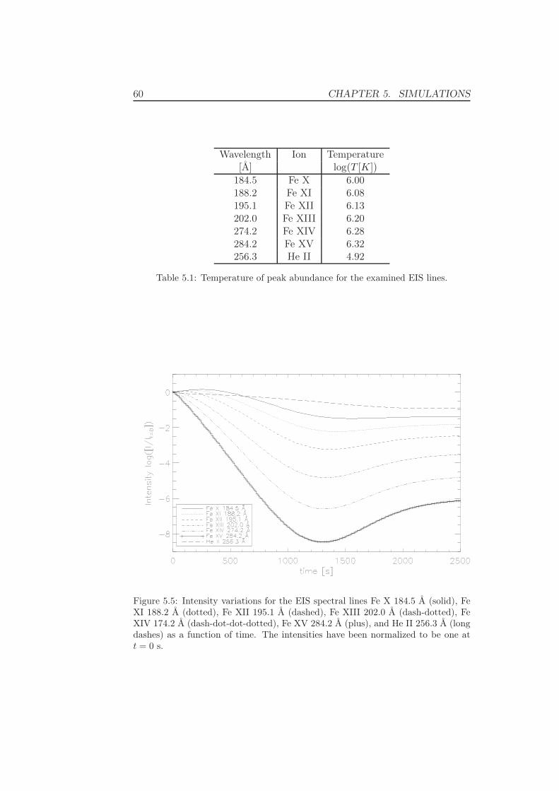
60 CHAPTER 5. SIMULATIONS
Wavelength Ion Temperature[Å] log(T [K])
184.5 Fe X 6.00188.2 Fe XI 6.08195.1 Fe XII 6.13202.0 Fe XIII 6.20274.2 Fe XIV 6.28284.2 Fe XV 6.32256.3 He II 4.92
Table 5.1: Temperature of peak abundance for the examined EIS lines.
Figure 5.5: Intensity variations for the EIS spectral lines Fe X 184.5 Å (solid), FeXI 188.2 Å (dotted), Fe XII 195.1 Å (dashed), Fe XIII 202.0 Å (dash-dotted), FeXIV 174.2 Å (dash-dot-dot-dotted), Fe XV 284.2 Å (plus), and He II 256.3 Å (longdashes) as a function of time. The intensities have been normalized to be one att = 0 s.
5.2. WARM LOOP COOLING 61
When the loop has stabilized after 2500 s, the intensity of the first line hasbeen reduced by a factor 30 compared to its level at the onset of the simu-lation, the second has fallen by two orders of magnitude, and the third bythree orders of magnitude.
The three hotter iron lines Fe XIII 202.0 Å, Fe XIV 274.2 Å, andFe XV 284.2 Å are also plotted in Figure 5.5. These lines start decreasing inintensity immediately, with the ion of highest temperature of peak abundancefalling very rapidly indeed. All these lines have a minimum after about1300 s, when the coolest (202.0) has been reduced by five orders of magnitudewhile the warmest (284.2) has been reduced by nine orders of magnitude.When the loop has stabilized after 2500 s, the 202.0 line has fallen by fourorders of magnitude compared to the onset of the simulation, the 274.2 lineis reduced by five orders of magnitude, and the 284.2 line by six orders ofmagnitude.
In contrast, the He II 256.3 Å, which is formed in the lower transitionregion, shows fairly small variations in intensity. This line is plotted withlong dashes in Figure 5.5. The intensity of this line falls less than a factorten, and it has no distinct minimum at t ≈ 1300 s when the loop is at itsminimum temperature.
Let us now try to explain why these lines’ intensity changes as it does.The intensity is related to the number density in the upper level that con-tributes in the line formation (nu) as stated in Equation 2.2,
Iν =hν
4π
∫ s
0nuAul φν ds .
When coronal equilibrium is valid, nu should relate to the temperature anddensity as (cf. Equation 2.12)
nu = nlneClu
Aul∝ ρ2f(T ) . (5.3)
We will now try to explain the variations in nu by the changes in temperatureand density, and examine whether these variations relate to the changes inthe lines’ intensity.
The number density of the upper level of the three iron lines whichstart by increasing in intensity the first few hundred seconds, Fe X 184.5 Å,Fe XI 188.2 Å, and Fe XII 195.1 Å, are plotted in the upper left, upper right,and middle left panels of Figure 5.6, respectively. At time t = 0 s these linesare mostly formed in the transition region and lower corona. After 40 s,the number density in each of the upper levels has barely decreased in theseregions while it has increased substantially in the corona, where the temper-ature is falling rapidly. In total nu for these lines has increased (or at leastnot decreased), resulting in a stronger emission from these lines.
The temperature keeps falling, and is reduced to 1 MK after 500 s. Inthe mean time, the number density population has continued to fall of in
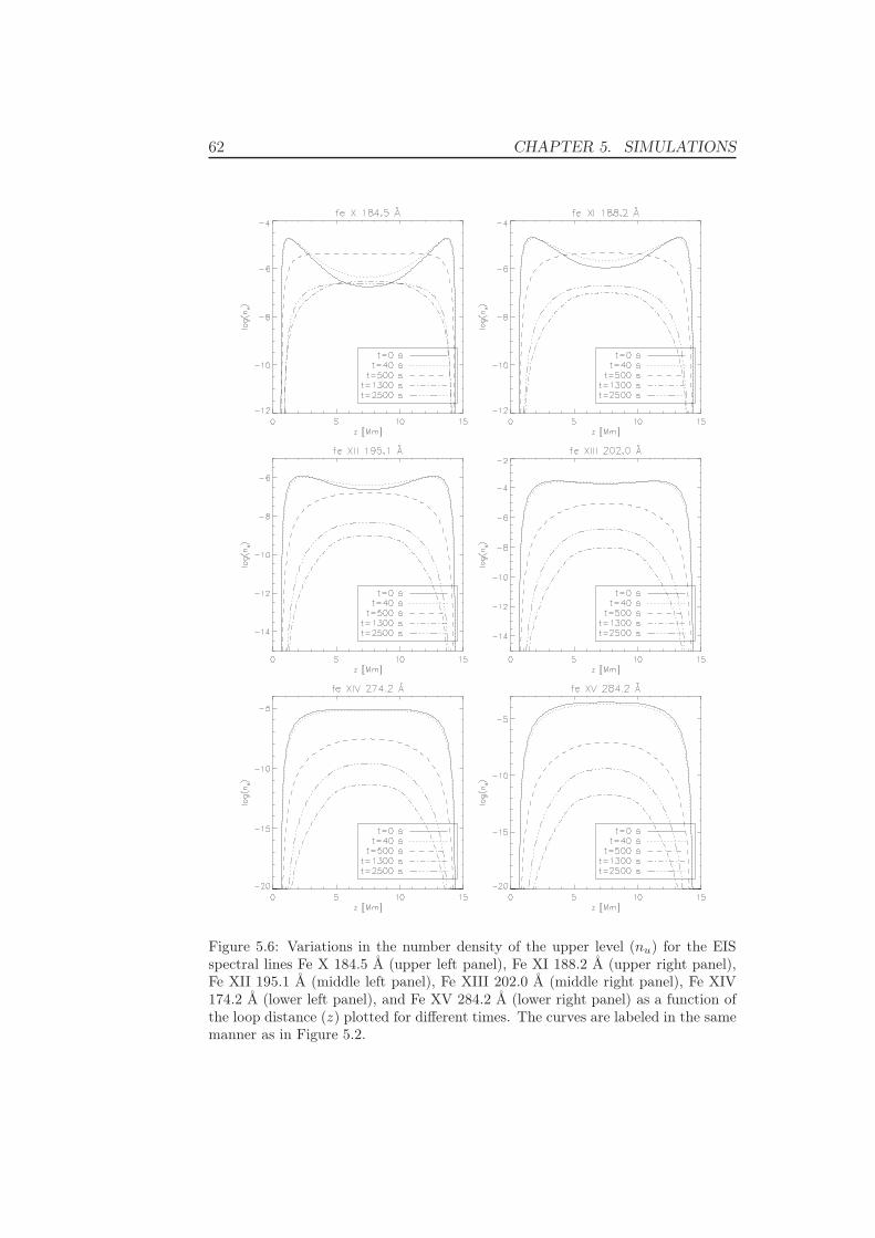
62 CHAPTER 5. SIMULATIONS
Figure 5.6: Variations in the number density of the upper level (nu) for the EISspectral lines Fe X 184.5 Å (upper left panel), Fe XI 188.2 Å (upper right panel),Fe XII 195.1 Å (middle left panel), Fe XIII 202.0 Å (middle right panel), Fe XIV174.2 Å (lower left panel), and Fe XV 284.2 Å (lower right panel) as a function ofthe loop distance (z) plotted for different times. The curves are labeled in the samemanner as in Figure 5.2.
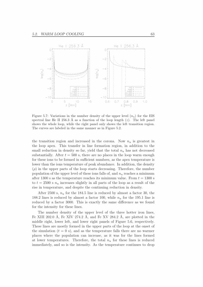
5.2. WARM LOOP COOLING 63
Figure 5.7: Variations in the number density of the upper level (nu) for the EISspectral line He II 256.3 Å as a function of the loop length (z). The left panelshows the whole loop, while the right panel only shows the left transition region.The curves are labeled in the same manner as in Figure 5.2.
the transition region and increased in the corona. Now nu is greatest inthe loop apex. This transfer in line formation region, in addition to thesmall reduction in density so far, yield that the total nu has not decreasedsubstantially. After t = 500 s, there are no places in the loop warm enoughfor these ions to be formed in sufficient numbers, as the apex temperature islower than the ions temperature of peak abundance. In addition, the density(ρ) in the upper parts of the loop starts decreasing. Therefore, the numberpopulation of the upper level of these ions falls of, and nu reaches a minimumafter 1300 s as the temperature reaches its minimum value. From t = 1300 sto t = 2500 s nu increases slightly in all parts of the loop as a result of therise in temperature, and despite the continuing reduction in density.
After 2500 s, nu for the 184.5 line is reduced by almost a factor 30, the188.2 lines is reduced by almost a factor 100, while nu for the 195.1 line isreduced by a factor 3000. This is exactly the same difference as we foundfor the intensity for these lines.
The number density of the upper level of the three hotter iron lines,Fe XIII 202.0 Å, Fe XIV 274.2 Å, and Fe XV 284.2 Å, are plotted in themiddle right, lower left, and lower right panels of Figure 5.6, respectively.These lines are mostly formed in the upper parts of the loop at the onset ofthe simulation (t = 0 s), and as the temperature falls there are no warmerplaces where the population can increase, as it was for the lines formedat lower temperatures. Therefore, the total nu for these lines is reducedimmediately, and so is the intensity. As the temperature continues to drop
64 CHAPTER 5. SIMULATIONS
off and the density is reduced substantially in the upper parts of the loop, nu
continues to decrease. This causes the intensity to fall of by a large numberof magnitudes and the lines to essentially disappear.
The number density of the upper level of the transition region He II256.3 Å line is plotted in Figure 5.7. This line is mostly formed in thetransition region, but also partly in the corona. Therefore, we plot nu fordifferent times as a function of the loop distance in the left panel, whilein the right panel we focus on the left footpoint transition region only. Asthe loop cools, its apex never reaches the temperature of peak abundancefor the helium line at 104.9 K. Therefore, the reduction in temperature doesnot effect the nu-population as much as for the iron lines. This causes theintensity to decrease as the density goes down, but in much less degree thanthe iron lines. After 2500 s, nu for this line has been reduced by almosta factor ten, which is the same as the reduction in intensity. The movingtransition region is clearly visible in the right panel of Figure 5.7.
Doppler Velocity
The Doppler velocity for the lines discussed above is plotted in Figure 5.8.Each line shows a sum of the two velocity signals, that is, the sound wavewith period of 100 s and on longer time-scales the mass flow from the apexand down into the footpoints.
The velocity is different for the different lines, with the iron ions withlowest temperature of peak abundance having the greatest negative velocitiesthe first 500 s, and after this the helium line has greatest negative velocity.The maximum velocity of the plasma movement along the loop was foundin the previous section to be after 1300 s, which is almost the same time asthe maximum Doppler velocity measured by the helium line. The iron lineson the other hand, do not show an exact minimum but have their greatestnegative velocity from 400 to 700 s after the onset of the simulation. Thereason for this is that in the beginning of the simulation, the plasma velocityis greatest in the corona, where the iron lines are formed. As time passesthe region of the maximum velocity is moving down into the lower coronaand transition region, where the helium line is formed. This can be seen inthe right panel of Figure 5.3. Therefore, the velocity of this line is rising(negatively) as long as the loop velocity is increasing. The iron lines, on theother hand, stop increasing as the plasma velocity peak passes the regionof their peak abundance. In addition, the lines with lowest temperature ofpeak abundance are formed more in the lower regions of the loop, where thevelocities contribute more to the line of sight velocity.
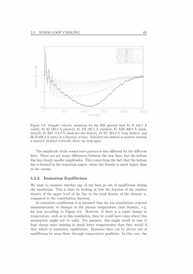
5.2. WARM LOOP COOLING 65
Figure 5.8: Doppler velocity variations for the EIS spectral lines Fe X 184.5 Å(solid), Fe XI 188.2 Å (dotted), Fe XII 195.1 Å (dashed), Fe XIII 202.0 Å (dash-dotted), Fe XIV 174.2 Å (dash-dot-dot-dotted), Fe XV 284.2 Å (long dashes), andHe II 256.3 Å (plus) as a function of time. Velocities are defined as positive towardsa detector situated vertically above the loop apex.
The amplitude of the sound wave pattern is also different for the differentlines. There are not many differences between the iron lines, but the heliumline has clearly smaller amplitudes. This comes from the fact that the heliumline is formed in the transition region, where the density is much higher thanin the corona.
5.2.3 Ionization Equilibrium
We want to examine whether any of our lines go out of equilibrium duringthe simulation. This is done by looking at how the fraction of the numberdensity of the upper level of the line to the total density of the element is,compared to the contribution function.
In ionization equilibrium it is assumed that the ion populations respondinstantaneously to changes in the plasma temperature (and density), e.g.for iron according to Figure 4.6. However, if there is a rapid change intemperature, such as in this simulation, then we could have cases where thisassumption might not be valid. For instance, this might result in ions ofhigh charge state existing at much lower temperatures than they would ifthey where in ionization equilibrium. Emission lines can be driven out ofequilibrium by mass flows through temperature gradients. In this case, the

66 CHAPTER 5. SIMULATIONS
Figure 5.9: Variations in the ratio of the number density of the upper level (nu)to the total number density of iron (nfe) for the EIS spectral lines as a function oftemperature and for different times. Fe X 184.5 Å (upper left panel), Fe XI 188.2Å (upper right panel), Fe XII 195.1 Å (middle left panel), Fe XIII 202.0 Å (middleright panel), Fe XIV 174.2 Å (lower left panel), and Fe XV 284.2 Å (lower rightpanel). The curves are labeled in the same manner as in Figure 5.2. All panels areover-plotted by the contribution function of the line (plus) in arbitrary units.
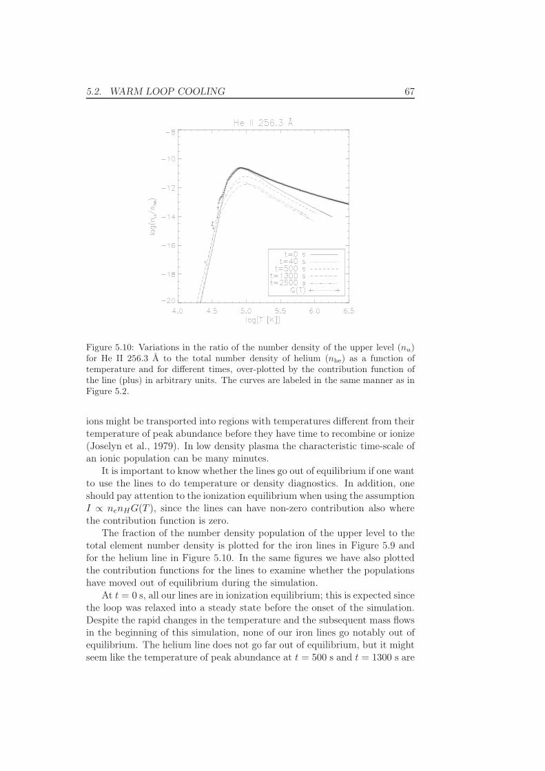
5.2. WARM LOOP COOLING 67
Figure 5.10: Variations in the ratio of the number density of the upper level (nu)for He II 256.3 Å to the total number density of helium (nhe) as a function oftemperature and for different times, over-plotted by the contribution function ofthe line (plus) in arbitrary units. The curves are labeled in the same manner as inFigure 5.2.
ions might be transported into regions with temperatures different from theirtemperature of peak abundance before they have time to recombine or ionize(Joselyn et al., 1979). In low density plasma the characteristic time-scale ofan ionic population can be many minutes.
It is important to know whether the lines go out of equilibrium if one wantto use the lines to do temperature or density diagnostics. In addition, oneshould pay attention to the ionization equilibrium when using the assumptionI ∝ nenHG(T ), since the lines can have non-zero contribution also wherethe contribution function is zero.
The fraction of the number density population of the upper level to thetotal element number density is plotted for the iron lines in Figure 5.9 andfor the helium line in Figure 5.10. In the same figures we have also plottedthe contribution functions for the lines to examine whether the populationshave moved out of equilibrium during the simulation.
At t = 0 s, all our lines are in ionization equilibrium; this is expected sincethe loop was relaxed into a steady state before the onset of the simulation.Despite the rapid changes in the temperature and the subsequent mass flowsin the beginning of this simulation, none of our iron lines go notably out ofequilibrium. The helium line does not go far out of equilibrium, but it mightseem like the temperature of peak abundance at t = 500 s and t = 1300 s are
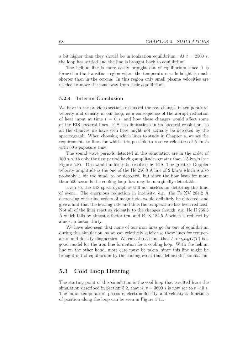
68 CHAPTER 5. SIMULATIONS
a bit higher than they should be in ionization equilibrium. At t = 2500 s,the loop has settled and the line is brought back to equilibrium.
The helium line is more easily brought out of equilibrium since it isformed in the transition region where the temperature scale height is muchshorter than in the corona. In this region only small plasma velocities areneeded to move the ions away from their equilibrium.
5.2.4 Interim Conclusion
We have in the previous sections discussed the real changes in temperature,velocity and density in our loop, as a consequence of the abrupt reductionof heat input at time t = 0 s, and how these changes would affect someof the EIS spectral lines. EIS has limitations in its spectral resolution, soall the changes we have seen here might not actually be detected by thespectrograph. When choosing which lines to study in Chapter 4, we set therequirements to lines for which it is possible to resolve velocities of 5 km/swith 60 s exposure time.
The sound wave periods detected in this simulation are in the order of100 s, with only the first period having amplitudes greater than 1.5 km/s (seeFigure 5.8). This would unlikely be resolved by EIS. The greatest Dopplervelocity amplitude is the one of the He 256.3 Å line of 2 km/s which is alsoprobably a bit too small to be detected, but since the flow lasts for morethan 500 seconds the cooling loop flow may be marginally detectable.
Even so, the EIS spectrograph is still not useless for detecting this kindof event. The enormous reduction in intensity, e.g. the Fe XV 284.2 Ådecreasing with nine orders of magnitude, would definitely be detected, andgive a hint that the heating rate and thus the temperature has been reduced.Not all of the lines react as violently to the changes though, e.g. He II 256.3Å which falls by almost a factor ten, and Fe X 184.5 Å which is reduced byalmost a factor thirty.
We have also seen that none of our iron lines go far out of equilibriumduring this simulation, so we can relatively safely use these lines for temper-ature and density diagnostics. We can also assume that I ∝ nenHG(T ) is agood model for the iron line formation for a cooling loop. With the heliumline on the other hand, more care must be taken, since this line might bebrought out of equilibrium by the cooling event that defines this simulation.
5.3 Cold Loop Heating
The starting point of this simulation is the cool loop that resulted from thesimulation described in Section 5.2, that is, t = 3600 s is now set to t = 0 s.The initial temperature, pressure, electron density, and velocity as functionsof position along the loop can be seen in Figure 5.11.

5.3. COLD LOOP HEATING 69
Figure 5.11: Left panel: The initial distribution of temperature (solid), pressure(dashed) and electron density (dotted) with distance (z) along loop. Right panel:The initial velocity distribution with distance (z) along loop.
The temperature is of order 6000 K in the loop footpoints extendingalmost 1 Mm up before the rapid transition region temperature rise is en-countered. Here, at z ≈ 0.8 Mm, the temperature rises to almost 1 MK overa few Mm. This temperature structure is maintained by an input heat fluxof 60 W/m2 in both sides of the loop, deposited from zleft
0 = 4.5 Mm andzright0 = 10.5 Mm, with a scale height zleft
H = zrightH = 4.0 Mm. The electron
density starts out at 3 × 10¹⁸ m−3 in the footpoints, decreasing to 2 × 10¹⁷
m−3 in the upper part of the chromosphere. In the transition region thedensity drops of even more, and continues to decrease down to 1015 m−3 inthe corona.
The pressure starts of at 100 Pa in the footpoints, decreasing rapidly toless than 0.05 Pa, until the end of the transition region. As the temperaturerises, the pressure scale height increases, and the pressure is almost constantthrough the upper part of the loop. As seen in the right panel of Figure5.11, the velocity is nearly zero through the entire initial model. At t = 0 swe change the heating flux back to what it was before the cooling startedin the previous section, namely 6000 W/m2, and start our new experiment.No other changes are made.
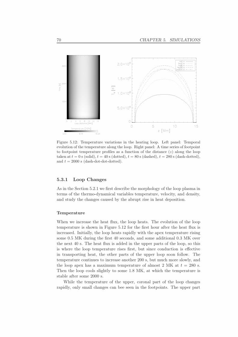
70 CHAPTER 5. SIMULATIONS
Figure 5.12: Temperature variations in the heating loop. Left panel: Temporalevolution of the temperature along the loop. Right panel: A time series of footpointto footpoint temperature profiles as a function of the distance (z) along the looptaken at t = 0 s (solid), t = 40 s (dotted), t = 80 s (dashed), t = 280 s (dash-dotted),and t = 2000 s (dash-dot-dot-dotted).
5.3.1 Loop Changes
As in the Section 5.2.1 we first describe the morphology of the loop plasma interms of the thermo-dynamical variables temperature, velocity, and density,and study the changes caused by the abrupt rise in heat deposition.
Temperature
When we increase the heat flux, the loop heats. The evolution of the looptemperature is shown in Figure 5.12 for the first hour after the heat flux isincreased. Initially, the loop heats rapidly with the apex temperature risingsome 0.5 MK during the first 40 seconds, and some additional 0.3 MK overthe next 40 s. The heat flux is added in the upper parts of the loop, so thisis where the loop temperature rises first, but since conduction is effectivein transporting heat, the other parts of the upper loop soon follow. Thetemperature continues to increase another 200 s, but much more slowly, andthe loop apex has a maximum temperature of almost 2 MK at t = 280 s.Then the loop cools slightly to some 1.8 MK, at which the temperature isstable after some 2000 s.
While the temperature of the upper, coronal part of the loop changesrapidly, only small changes can bee seen in the footpoints. The upper part

5.3. COLD LOOP HEATING 71
Figure 5.13: Velocity variations in the heating loop. Left panel: Temporal evolutionof the velocity along the loop. Right panel: A time series of footpoint to footpointvelocity profiles as a function of the distance (z) along the loop. The curves arelabeled in the same manner as in Figure 5.12.
of the chromosphere heats up slightly, moving the bottom of the transitionregion downwards some 0.2 Mm.
Velocity
Also in this experiment does the change in heat input affect the velocitiesin the plasma, and this time more violently and on shorter time-scales thanin the previous experiment. The loop velocities for the first hour of thesimulation can be seen in Figure 5.13. The left panel of this figure shows awave pattern the first 300 s, and a mass flux from the footpoints towards theapex during the first 1500–2000 s.
The rapidly increasing temperature in the loop apex causes an increasedpressure which creates a sound wave propagating from the loop apex anddown towards the footpoints. With a pressure of ∼ 0.05 Pa and density of∼ 10−12 kg/m3 we get a sound velocity of some 100 km/s. As in the previousexperiment the wave is being reflected when it reaches the transition regiondue to the rapid change in sound speed. The wave amplitude reaches itsmaximum of 20 km/s after 80 s, and thereafter it is being quickly damped.The left panel of Figure 5.13 shows only three oscillations, with a period ofabout 100 s. As in the previous experiment the wave is damped presumablydue to leakage into the transition region or by radiative damping. Theoscillations disappear in the lower parts of the loop first, because of the

72 CHAPTER 5. SIMULATIONS
Figure 5.14: Density variations in the heating loop. Left panel: Temporal evolutionof the density along the loop. Right panel: A time series of footpoint to footpointdensity profiles as a function of the distance (z) along the loop. The curves arelabeled in the same manner as in Figure 5.12.
higher density. As noted above, the plasma is first moving downwards, butas the loop heats it is able to support more mass, causing the material toflow upwards. This mass flux lasts some 2000 s, with continuously decreasingvelocity.
Density
As can be seen in Figure 5.14, the density is almost constant the first 80seconds, except for a small decrease around the loop apex and increase inthe lower part of the corona. From 80 s the density is increasing through allof the upper parts of the loop, with the apex value increasing with a factorfour, from log(ρ) = −11.4 at t = 0 s to log(ρ) = −10.8 at t = 3600 s. As inthe previous experiment, only small changes are seen in the density structureof the transition region and none is seen in the chromosphere.
The increased density causes the loop heating to stabilize and the loopcools slightly after 280 s. This is the opposite effect of what was seen in theprevious experiment.
5.3.2 The EIS Lines’ Response to the Changes
Now we take a look at what happen to the EIS spectral lines as a result of theloop changes in temperature, density, and velocity as described above. The
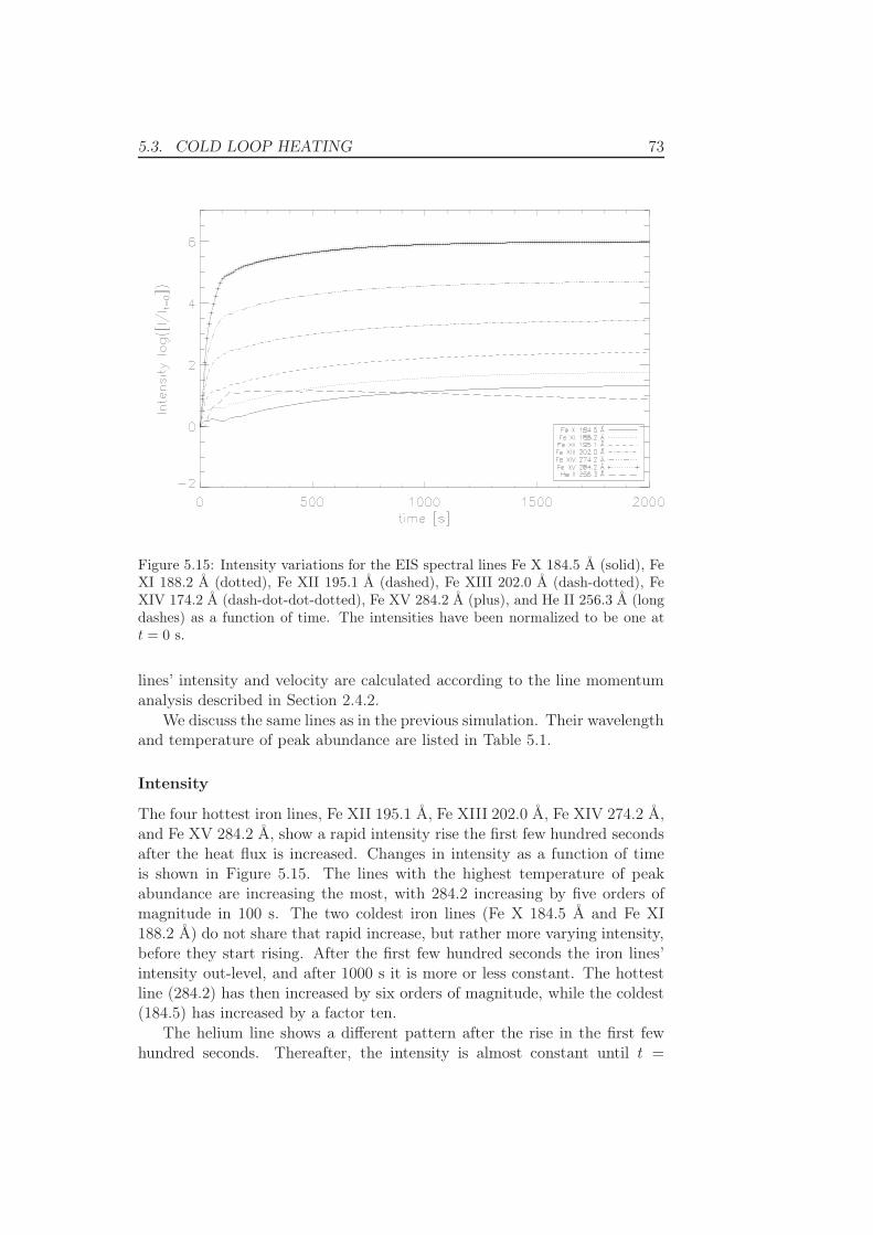
5.3. COLD LOOP HEATING 73
Figure 5.15: Intensity variations for the EIS spectral lines Fe X 184.5 Å (solid), FeXI 188.2 Å (dotted), Fe XII 195.1 Å (dashed), Fe XIII 202.0 Å (dash-dotted), FeXIV 174.2 Å (dash-dot-dot-dotted), Fe XV 284.2 Å (plus), and He II 256.3 Å (longdashes) as a function of time. The intensities have been normalized to be one att = 0 s.
lines’ intensity and velocity are calculated according to the line momentumanalysis described in Section 2.4.2.
We discuss the same lines as in the previous simulation. Their wavelengthand temperature of peak abundance are listed in Table 5.1.
Intensity
The four hottest iron lines, Fe XII 195.1 Å, Fe XIII 202.0 Å, Fe XIV 274.2 Å,and Fe XV 284.2 Å, show a rapid intensity rise the first few hundred secondsafter the heat flux is increased. Changes in intensity as a function of timeis shown in Figure 5.15. The lines with the highest temperature of peakabundance are increasing the most, with 284.2 increasing by five orders ofmagnitude in 100 s. The two coldest iron lines (Fe X 184.5 Å and Fe XI188.2 Å) do not share that rapid increase, but rather more varying intensity,before they start rising. After the first few hundred seconds the iron lines’intensity out-level, and after 1000 s it is more or less constant. The hottestline (284.2) has then increased by six orders of magnitude, while the coldest(184.5) has increased by a factor ten.
The helium line shows a different pattern after the rise in the first fewhundred seconds. Thereafter, the intensity is almost constant until t =

74 CHAPTER 5. SIMULATIONS
500 s, and then it falls of slowly the rest of the simulation, ending up havingincreased by less than a factor ten.
As in the previous experiment, we take a look at the number density ofthe upper level that contributes to each of the lines and examine whether thechanges in this variable relates to the changes in density and temperature,and if it can explain the variations in intensity. nu is plotted for the ironlines in Figure 5.16 and for the helium line in Figure 5.17.
At the onset of the simulation, the two coldest iron lines, Fe X 184.5 Åand Fe XI 188.2 Å, are formed mainly in the upper parts of the loop. nu forthese lines is plotted in the upper left and upper middle panel of Figure 5.16,respectively. As the temperature starts rising, the lower corona is gettingwarm enough and the upper corona is getting too warm for these ions tobe formed in sufficient numbers. Therefore, the number density falls in theloop apex and increases in the transition region and lower corona. Thesechanges cause the varying intensity the first 100 s for these lines. As thedensity starts increasing after 80 s, nu increases in all parts of the loop, andthe intensity starts rising. At the end of the simulation, nu for the 184.5 linehas increased by a factor ten and for the 188.2 line by a factor hundred.
The number density of the upper level of the four hotter iron lines,Fe XII 195.1 Å, Fe XIII 202.0 Å, Fe XIV 274.2 Å, and Fe XV 284.2 Å,increases all over the loop. nu for these lines is plotted in the middle left,middle right, lower left, and lower right panels of Figure 5.16, respectively.The lines nu increases rapidly in the beginning of the simulation, because ofthe enormous rise in temperature. This explains the rapid intensity growthduring the first 100 s of the simulation. The 195.1, 202.0 and 274.2 lines geta small ’bump’ at the apex at t = 280 s, probably because of the temperaturethere being greater than their temperature of peak abundance. nu continuesto increase after t = 280 s, even if the temperature goes down, since thedensity is still rising. At the end of the simulation, nu for the 284.2 line hasincreased by six orders of magnitude, the 274.2 by five orders of magnitude,the 202.0 line by three orders of magnitude, and the 195.1 line by two ordersof magnitude. This matches the intensity variations.
The number density of the upper level of the He 256.3 Å line is plottedin Figure 5.17. The peak abundance of this line is at 104.9 K, but thecontribution function is non-zero up until 106 K (cf. Figure 4.4). As thetemperature rises in the loop apex, nu decreases there, which can be seen inthe left panel of the figure. At the same time, nu increases in the transitionregion and lower corona, so that in total nu increases. After 80 s the densitystarts rising, causing nu, and thus the intensity, to increase even further. nu
is increasing the first 280 s, and then decreases slightly as the temperaturefalls. nu increases from t = 0 s to t = 2500 s by almost a factor ten, which isthe same as for the intensity. The moving transition region is clearly visiblein the right panel of Figure 5.17.
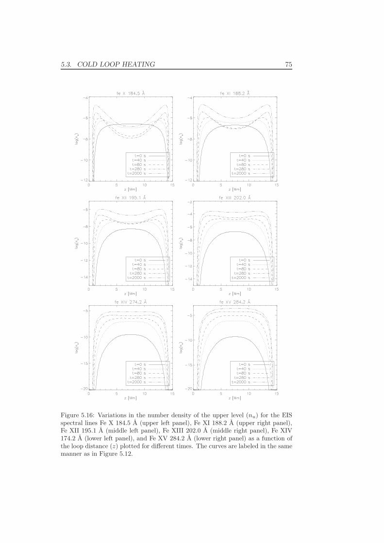
5.3. COLD LOOP HEATING 75
Figure 5.16: Variations in the number density of the upper level (nu) for the EISspectral lines Fe X 184.5 Å (upper left panel), Fe XI 188.2 Å (upper right panel),Fe XII 195.1 Å (middle left panel), Fe XIII 202.0 Å (middle right panel), Fe XIV174.2 Å (lower left panel), and Fe XV 284.2 Å (lower right panel) as a function ofthe loop distance (z) plotted for different times. The curves are labeled in the samemanner as in Figure 5.12.
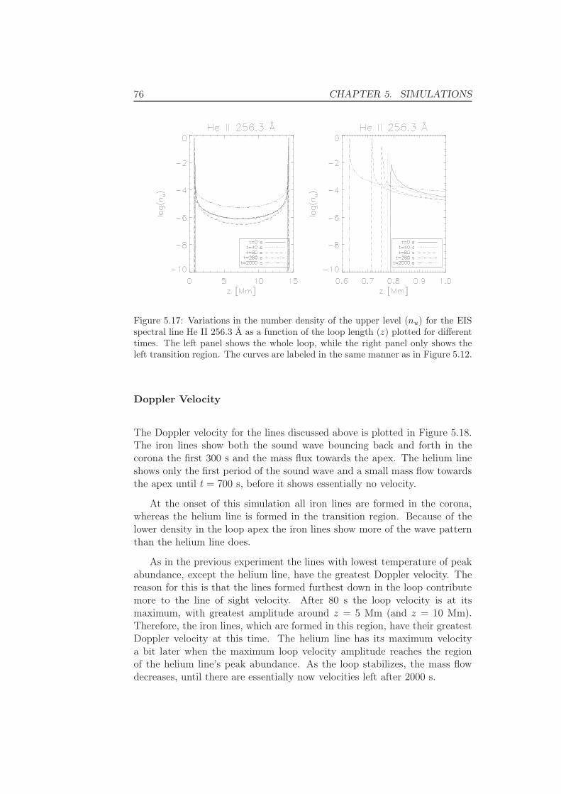
76 CHAPTER 5. SIMULATIONS
Figure 5.17: Variations in the number density of the upper level (nu) for the EISspectral line He II 256.3 Å as a function of the loop length (z) plotted for differenttimes. The left panel shows the whole loop, while the right panel only shows theleft transition region. The curves are labeled in the same manner as in Figure 5.12.
Doppler Velocity
The Doppler velocity for the lines discussed above is plotted in Figure 5.18.The iron lines show both the sound wave bouncing back and forth in thecorona the first 300 s and the mass flux towards the apex. The helium lineshows only the first period of the sound wave and a small mass flow towardsthe apex until t = 700 s, before it shows essentially no velocity.
At the onset of this simulation all iron lines are formed in the corona,whereas the helium line is formed in the transition region. Because of thelower density in the loop apex the iron lines show more of the wave patternthan the helium line does.
As in the previous experiment the lines with lowest temperature of peakabundance, except the helium line, have the greatest Doppler velocity. Thereason for this is that the lines formed furthest down in the loop contributemore to the line of sight velocity. After 80 s the loop velocity is at itsmaximum, with greatest amplitude around z = 5 Mm (and z = 10 Mm).Therefore, the iron lines, which are formed in this region, have their greatestDoppler velocity at this time. The helium line has its maximum velocitya bit later when the maximum loop velocity amplitude reaches the regionof the helium line’s peak abundance. As the loop stabilizes, the mass flowdecreases, until there are essentially now velocities left after 2000 s.
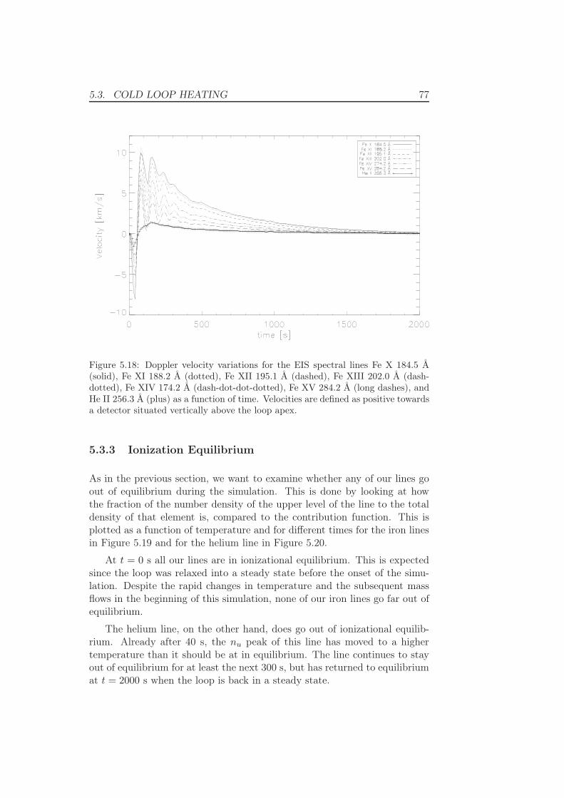
5.3. COLD LOOP HEATING 77
Figure 5.18: Doppler velocity variations for the EIS spectral lines Fe X 184.5 Å(solid), Fe XI 188.2 Å (dotted), Fe XII 195.1 Å (dashed), Fe XIII 202.0 Å (dash-dotted), Fe XIV 174.2 Å (dash-dot-dot-dotted), Fe XV 284.2 Å (long dashes), andHe II 256.3 Å (plus) as a function of time. Velocities are defined as positive towardsa detector situated vertically above the loop apex.
5.3.3 Ionization Equilibrium
As in the previous section, we want to examine whether any of our lines goout of equilibrium during the simulation. This is done by looking at howthe fraction of the number density of the upper level of the line to the totaldensity of that element is, compared to the contribution function. This isplotted as a function of temperature and for different times for the iron linesin Figure 5.19 and for the helium line in Figure 5.20.
At t = 0 s all our lines are in ionizational equilibrium. This is expectedsince the loop was relaxed into a steady state before the onset of the simu-lation. Despite the rapid changes in temperature and the subsequent massflows in the beginning of this simulation, none of our iron lines go far out ofequilibrium.
The helium line, on the other hand, does go out of ionizational equilib-rium. Already after 40 s, the nu peak of this line has moved to a highertemperature than it should be at in equilibrium. The line continues to stayout of equilibrium for at least the next 300 s, but has returned to equilibriumat t = 2000 s when the loop is back in a steady state.
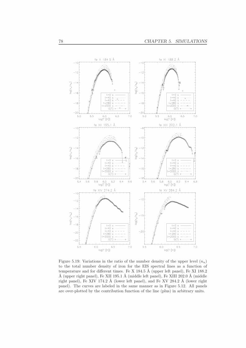
78 CHAPTER 5. SIMULATIONS
Figure 5.19: Variations in the ratio of the number density of the upper level (nu)to the total number density of iron for the EIS spectral lines as a function oftemperature and for different times. Fe X 184.5 Å (upper left panel), Fe XI 188.2Å (upper right panel), Fe XII 195.1 Å (middle left panel), Fe XIII 202.0 Å (middleright panel), Fe XIV 174.2 Å (lower left panel), and Fe XV 284.2 Å (lower rightpanel). The curves are labeled in the same manner as in Figure 5.12. All panelsare over-plotted by the contribution function of the line (plus) in arbitrary units.

5.3. COLD LOOP HEATING 79
Figure 5.20: Variations in the ratio of the number density of the upper level (nu)for He II 256.3 Å to the total number density of helium as a function of temperatureand for different times, over-plotted by the contribution function of the line (plus)in arbitrary units. The curves are labeled in the same manner as in Figure 5.12.
5.3.4 Interim Conclusion
We have in the previous sections discussed the real changes in temperature,velocity and density in our loop model, as a consequence of the abrupt in-crease of heat input at time t = 0 s, and how these changes affect some ofthe EIS spectral lines. It is now time to discuss which of these changes EISwould actually be able to detect.
The iron lines, and especially those with low temperature of peak abund-ance, show great Doppler velocity amplitudes the first few hundred secondsafter the onset of the simulation. The detector will probably be able to de-tect these mass flow velocities of more than 5 km/s, but not likely noticethe sound wave signal because of the rapid amplitude damping. EIS will notbe able to detect the Doppler velocities of the helium line and the iron lineswith highest temperature of peak abundance. The great intensity increase inthe iron lines will surely be noted by EIS. The Fe 284.2 Å line increases withfive orders of magnitude in only 100 s. The helium line and the iron lineswith low temperature of peak abundance do not have this violent increase inintensity. The He II 256.3 Å and Fe X 184.5 Å increase by about an orderof magnitude. Both the Doppler velocity and the intensity increase wouldindicate a change in the heating rate, causing the temperature in the loopto rise.
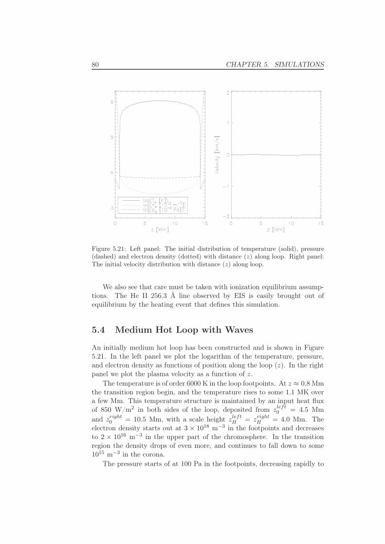
80 CHAPTER 5. SIMULATIONS
Figure 5.21: Left panel: The initial distribution of temperature (solid), pressure(dashed) and electron density (dotted) with distance (z) along loop. Right panel:The initial velocity distribution with distance (z) along loop.
We also see that care must be taken with ionization equilibrium assump-tions. The He II 256.3 Å line observed by EIS is easily brought out ofequilibrium by the heating event that defines this simulation.
5.4 Medium Hot Loop with Waves
An initially medium hot loop has been constructed and is shown in Figure5.21. In the left panel we plot the logarithm of the temperature, pressure,and electron density as functions of position along the loop (z). In the rightpanel we plot the plasma velocity as a function of z.
The temperature is of order 6000 K in the loop footpoints. At z ≈ 0.8 Mmthe transition region begin, and the temperature rises to some 1.1 MK overa few Mm. This temperature structure is maintained by an input heat fluxof 850 W/m2 in both sides of the loop, deposited from zleft
0 = 4.5 Mmand zright
0 = 10.5 Mm, with a scale height zleftH = zright
H = 4.0 Mm. Theelectron density starts out at 3 × 10¹⁸ m−3 in the footpoints and decreasesto 2 × 10¹⁶ m−3 in the upper part of the chromosphere. In the transitionregion the density drops of even more, and continues to fall down to some1015 m−3 in the corona.
The pressure starts of at 100 Pa in the footpoints, decreasing rapidly to

5.4. MEDIUM HOT LOOP WITH WAVES 81
less than 0.1 Pa until the end of the transition region. As the temperaturerises, the pressure scale height increases and the pressure is almost constantthrough the upper parts of the loop. As seen in the right panel of Figure 5.21,the velocity is nearly zero through the entire initial model.
At time t = 0 we start forcing on waves from the left footpoint of theloop. To introduce the sound wave, the lower left boundary moves as a pistonwith velocity
u = uamp cos (2πfrt − π/2) , (5.4)
where t is the time, fr = 0.0056 Hz is the frequency (three minute oscilla-tion), and uamp = 0.7 km/s is the amplitude. No other changes are made.
5.4.1 Loop Changes
Now we describe the morphology of the loop plasma in terms of the thermo-dynamical variables temperature, velocity, and density, and study the changescaused by the forced oscillation.
Velocity
There are no movements in the loop at the onset of the simulation, butstarting at t = 0 s we force a wave from the left footpoint every 180 s. Theloop velocity the first hour of the simulation can be seen in the left panelof Figure 5.22. A wave can be seen traveling from left to right, the firststarting from the left transition region (z ∼ 1 Mm) after 100 s, and then anew wave starts every 180 seconds. At first, the velocity amplitude increasesfor each oscillation, but from t = 1000 s the amplitude is constant. The rightpanel of the same figure shows the footpoint to footpoint velocity profile asa function of the loop length for chosen time steps through one wave period.
The first wave is visible in the lower left part of the corona after 100 s.In the chromosphere the pressure is about 100 Pa and the density is about10−6 kg/m3, which yield a sound speed of some 10 km/s. With this speed itshould take about 60 s to pass trough the chromosphere, where the density ishigh, so the wave amplitude will be small and barely visible. In addition, withthe piston movement given in Equation 5.4, the first sound wave maximumoriginates in the left footpoint (z = 0) after some 45 s. Therefore, the waveis first visible when it reaches the corona after some 100 s, as is shown in theleft panel of Figure 5.22.
In the corona the pressure is about 0.07 Pa and the density is about5 × 10−12 kg/m3, which yield a sound speed of 150 km/s. As in the twoprevious experiments, the wave is reflected when it reaches the right footpointtransition region due to the rapid reduction in sound speed. With this soundspeed and a distance of some 13.5 Mm from one transition region to the other,it should take the wave about 180 s back and forth through the corona. Thisis exactly what is seen in the left panel of Figure 5.22; a new wave is starting
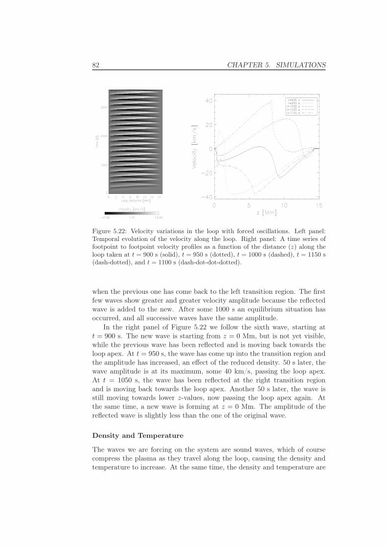
82 CHAPTER 5. SIMULATIONS
Figure 5.22: Velocity variations in the loop with forced oscillations. Left panel:Temporal evolution of the velocity along the loop. Right panel: A time series offootpoint to footpoint velocity profiles as a function of the distance (z) along theloop taken at t = 900 s (solid), t = 950 s (dotted), t = 1000 s (dashed), t = 1150 s(dash-dotted), and t = 1100 s (dash-dot-dot-dotted).
when the previous one has come back to the left transition region. The firstfew waves show greater and greater velocity amplitude because the reflectedwave is added to the new. After some 1000 s an equilibrium situation hasoccurred, and all successive waves have the same amplitude.
In the right panel of Figure 5.22 we follow the sixth wave, starting att = 900 s. The new wave is starting from z = 0 Mm, but is not yet visible,while the previous wave has been reflected and is moving back towards theloop apex. At t = 950 s, the wave has come up into the transition region andthe amplitude has increased, an effect of the reduced density. 50 s later, thewave amplitude is at its maximum, some 40 km/s, passing the loop apex.At t = 1050 s, the wave has been reflected at the right transition regionand is moving back towards the loop apex. Another 50 s later, the wave isstill moving towards lower z-values, now passing the loop apex again. Atthe same time, a new wave is forming at z = 0 Mm. The amplitude of thereflected wave is slightly less than the one of the original wave.
Density and Temperature
The waves we are forcing on the system are sound waves, which of coursecompress the plasma as they travel along the loop, causing the density andtemperature to increase. At the same time, the density and temperature are

5.4. MEDIUM HOT LOOP WITH WAVES 83
Figure 5.23: Density variations in the loop with forced waves. Left panel: Temporalevolution of the density along the loop. Right panel: A time series of footpoint tofootpoint density profiles as a function of the distance (z) along the loop. The linesare labeled as in Figure 5.22.
reduced in the tracks of the previous wave front, with a minimum 90 s afterthe maximum. The evolution of the loop density can be seen in Figure 5.23and the loop temperature in Figure 5.24. The left panels show the evolutionthe first hour after we started forcing on the waves, while the right panelsshow the footpoint to footpoint density and temperature, respectively, alongthe loop for some chosen times.
At t = 900 s, the previous wave has been reflected and is now movingtowards lower z-values. This can be seen by the density decrease in the lefthand side of the loop, in the tracks of the wave before it was reflected, andthe increased density around the wave at z = 10 Mm. No effect of the newwave that is forming can yet be seen in the left footpoint. The transitionregion is oscillating with a period of 180 s, moving some 0.3 Mm up and downfrom its starting point, which can be clearly seen in the left panel of Figure5.23. At t = 950 s, the new wave reaches the beginning of the transitionregion, where the density now is at its minimum. At t = 1000 s, the wavepasses the apex and increases the density there. As the wave is reflected, thewave amplitude in the left footpoint reaches its maximum. 50 s later, theincreased density due to the reflected wave can be seen at the right transitionregion. The reflected wave increases the density, but not as much as it didbefore it was reflected.
In addition to the increased density in the region of the wave peak, thereis always a temperature increase too, as can be seen in the right panel of

84 CHAPTER 5. SIMULATIONS
Figure 5.24: Temperature variations in the loop with forced oscillations. Left panel:Temporal evolution of the temperature along the loop. Right panel: A time seriesof footpoint to footpoint temperature profiles as a function of the distance (z) alongthe loop. The lines are labeled as in Figure 5.22.
Figure 5.24. The temperature increase is, as for the density, smaller whenit is the reflected wave that passes. The velocity amplitude is largest in theupper parts of the loop, where the density is smallest. The propagating waveamplitude, the reduced temperature in the tracks of the previous wave, andthe moving transition region is clearly seen in the temperature plot in theleft panel of the same figure.
5.4.2 The EIS Lines’ Response to the Changes
Now we take a look at how to the EIS spectral lines react to the loop changesin temperature, density, and velocity described above. The lines’ intensityand velocity now to be discussed are calculated according to the line mo-mentum analysis described in Section 2.4.2.
We are discussing the same lines as in the two previous experiments.Their wavelength and temperature of peak abundance are listed in Table5.1.
Intensity
The changes in the lines’ intensity as a function of time is shown in Figure5.25. All lines show oscillating intensities with periods of some 180 s. Theamplitudes are increasing for every new wave for the first 1000 s and then
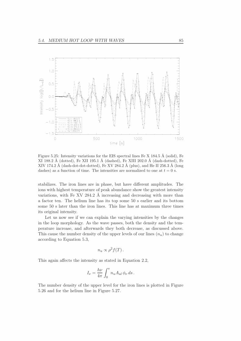
5.4. MEDIUM HOT LOOP WITH WAVES 85
Figure 5.25: Intensity variations for the EIS spectral lines Fe X 184.5 Å (solid), FeXI 188.2 Å (dotted), Fe XII 195.1 Å (dashed), Fe XIII 202.0 Å (dash-dotted), FeXIV 174.2 Å (dash-dot-dot-dotted), Fe XV 284.2 Å (plus), and He II 256.3 Å (longdashes) as a function of time. The intensities are normalized to one at t = 0 s.
stabilizes. The iron lines are in phase, but have different amplitudes. Theions with highest temperature of peak abundance show the greatest intensityvariations, with Fe XV 284.2 Å increasing and decreasing with more thana factor ten. The helium line has its top some 50 s earlier and its bottomsome 50 s later than the iron lines. This line has at maximum three timesits original intensity.
Let us now see if we can explain the varying intensities by the changesin the loop morphology. As the wave passes, both the density and the tem-perature increase, and afterwards they both decrease, as discussed above.This cause the number density of the upper levels of our lines (nu) to changeaccording to Equation 5.3,
nu ∝ ρ2f(T ) .
This again affects the intensity as stated in Equation 2.2,
Iν =hν
4π
∫ s
0nuAul φν ds .
The number density of the upper level for the iron lines is plotted in Figure5.26 and for the helium line in Figure 5.27.
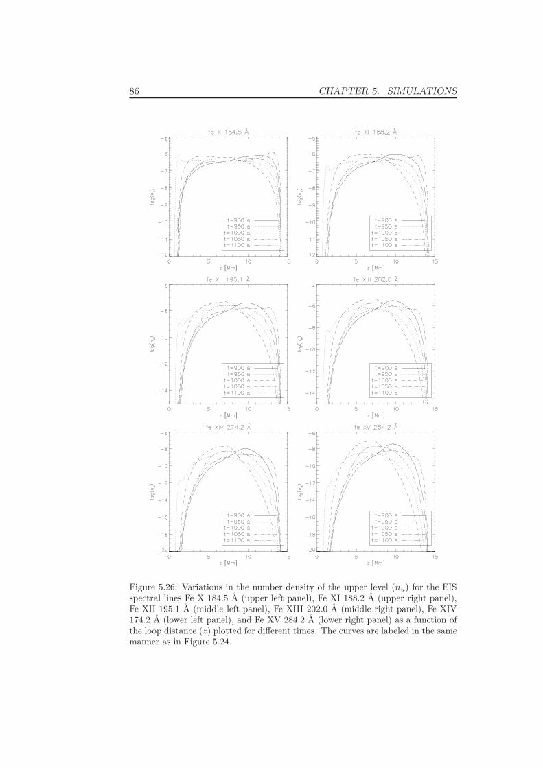
86 CHAPTER 5. SIMULATIONS
Figure 5.26: Variations in the number density of the upper level (nu) for the EISspectral lines Fe X 184.5 Å (upper left panel), Fe XI 188.2 Å (upper right panel),Fe XII 195.1 Å (middle left panel), Fe XIII 202.0 Å (middle right panel), Fe XIV174.2 Å (lower left panel), and Fe XV 284.2 Å (lower right panel) as a function ofthe loop distance (z) plotted for different times. The curves are labeled in the samemanner as in Figure 5.24.
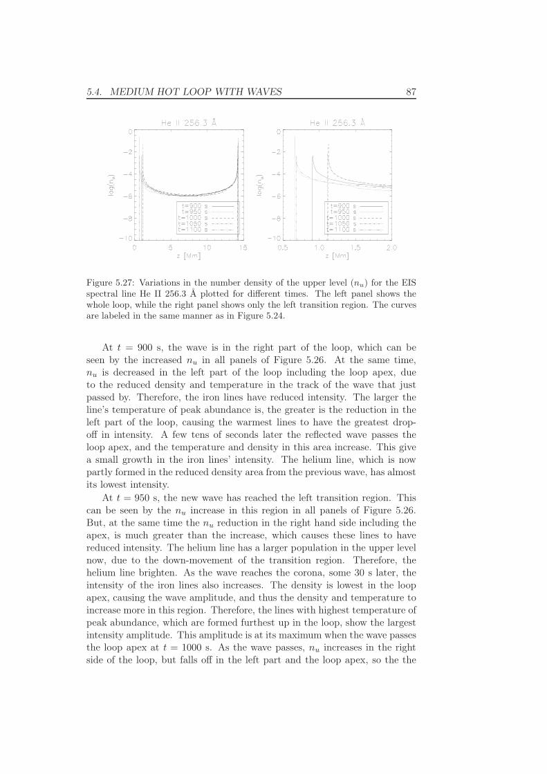
5.4. MEDIUM HOT LOOP WITH WAVES 87
Figure 5.27: Variations in the number density of the upper level (nu) for the EISspectral line He II 256.3 Å plotted for different times. The left panel shows thewhole loop, while the right panel shows only the left transition region. The curvesare labeled in the same manner as in Figure 5.24.
At t = 900 s, the wave is in the right part of the loop, which can beseen by the increased nu in all panels of Figure 5.26. At the same time,nu is decreased in the left part of the loop including the loop apex, dueto the reduced density and temperature in the track of the wave that justpassed by. Therefore, the iron lines have reduced intensity. The larger theline’s temperature of peak abundance is, the greater is the reduction in theleft part of the loop, causing the warmest lines to have the greatest drop-off in intensity. A few tens of seconds later the reflected wave passes theloop apex, and the temperature and density in this area increase. This givea small growth in the iron lines’ intensity. The helium line, which is nowpartly formed in the reduced density area from the previous wave, has almostits lowest intensity.
At t = 950 s, the new wave has reached the left transition region. Thiscan be seen by the nu increase in this region in all panels of Figure 5.26.But, at the same time the nu reduction in the right hand side including theapex, is much greater than the increase, which causes these lines to havereduced intensity. The helium line has a larger population in the upper levelnow, due to the down-movement of the transition region. Therefore, thehelium line brighten. As the wave reaches the corona, some 30 s later, theintensity of the iron lines also increases. The density is lowest in the loopapex, causing the wave amplitude, and thus the density and temperature toincrease more in this region. Therefore, the lines with highest temperature ofpeak abundance, which are formed furthest up in the loop, show the largestintensity amplitude. This amplitude is at its maximum when the wave passesthe loop apex at t = 1000 s. As the wave passes, nu increases in the rightside of the loop, but falls off in the left part and the loop apex, so the the
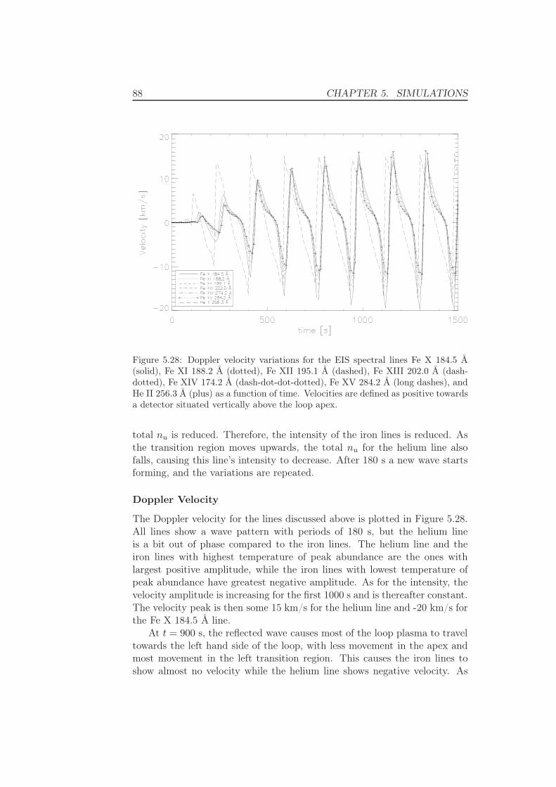
88 CHAPTER 5. SIMULATIONS
Figure 5.28: Doppler velocity variations for the EIS spectral lines Fe X 184.5 Å(solid), Fe XI 188.2 Å (dotted), Fe XII 195.1 Å (dashed), Fe XIII 202.0 Å (dash-dotted), Fe XIV 174.2 Å (dash-dot-dot-dotted), Fe XV 284.2 Å (long dashes), andHe II 256.3 Å (plus) as a function of time. Velocities are defined as positive towardsa detector situated vertically above the loop apex.
total nu is reduced. Therefore, the intensity of the iron lines is reduced. Asthe transition region moves upwards, the total nu for the helium line alsofalls, causing this line’s intensity to decrease. After 180 s a new wave startsforming, and the variations are repeated.
Doppler Velocity
The Doppler velocity for the lines discussed above is plotted in Figure 5.28.All lines show a wave pattern with periods of 180 s, but the helium lineis a bit out of phase compared to the iron lines. The helium line and theiron lines with highest temperature of peak abundance are the ones withlargest positive amplitude, while the iron lines with lowest temperature ofpeak abundance have greatest negative amplitude. As for the intensity, thevelocity amplitude is increasing for the first 1000 s and is thereafter constant.The velocity peak is then some 15 km/s for the helium line and -20 km/s forthe Fe X 184.5 Å line.
At t = 900 s, the reflected wave causes most of the loop plasma to traveltowards the left hand side of the loop, with less movement in the apex andmost movement in the left transition region. This causes the iron lines toshow almost no velocity while the helium line shows negative velocity. As

5.4. MEDIUM HOT LOOP WITH WAVES 89
Figure 5.29: Variations in the ratio of the number density of the upper level (nu)for He II 256.3 Å to the total number density of helium as a function of temperatureand for different times, over-plotted by the contribution function of the line (plus)in arbitrary units. The curves are labeled in the same manner as in Figure 5.24.
the wave passes the loop apex, the iron lines show negative velocity too.Some 40 s later, the new wave passes through the transition region wherethe helium line is formed. Thus, this line changes instantly from a negativeto a positive velocity. At this time the iron lines still show negative velocity,but a few tens of seconds later, when the wave reaches the area where theiron lines are formed, they get a positive velocity too. As the wave passesthe loop apex around t = 1000 s, all lines still have positive velocity, but theamplitudes are decreasing.
5.4.3 Ionization Equilibrium
As in the two previous experiments, we want to examine whether any of ourlines go out of equilibrium during the simulation. This is done by lookingat how the fraction of the number density of the upper level of the line tothe total density of that element is, compared to the contribution function.This is plotted as a function of temperature and for different times for theiron lines in Figure 5.30 and for the helium line in Figure 5.29.
At the onset of the simulations the loop is in a steady state and thus alllines are in ionization equilibrium. Despite the forced waves, with subsequentchanges in temperature and density, none of our iron lines go far out ofequilibrium. The helium line on the other hand, does go out of ionizational
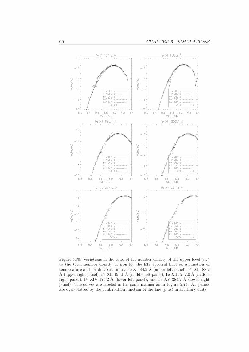
90 CHAPTER 5. SIMULATIONS
Figure 5.30: Variations in the ratio of the number density of the upper level (nu)to the total number density of iron for the EIS spectral lines as a function oftemperature and for different times. Fe X 184.5 Å (upper left panel), Fe XI 188.2Å (upper right panel), Fe XII 195.1 Å (middle left panel), Fe XIII 202.0 Å (middleright panel), Fe XIV 174.2 Å (lower left panel), and Fe XV 284.2 Å (lower rightpanel). The curves are labeled in the same manner as in Figure 5.24. All panelsare over-plotted by the contribution function of the line (plus) in arbitrary units.
5.4. MEDIUM HOT LOOP WITH WAVES 91
equilibrium. As the sound wave passes through the transition region, e.g.at t = 950 s, the greatest number density of He II ions is transported toa warmer part of the loop than it would normally be, because of the largetemperature gradient in this region. This is easily seen at t = 950 s inFigure 5.29. As the mass flow is reduced the helium line starts returning toequilibrium, and reaches it before t = 1050 s.
5.4.4 Interim Conclusion
We have in the previous sections discussed the real changes in temperature,velocity, and density in our loop as a result of the forced sound waves, andexamined how this would affect some of the EIS spectral lines. It is nowtime to discuss which of these changes EIS would actually be able to detect.
All our spectral lines show Doppler velocity oscillations with a period of180 s. With amplitudes of more than 10 km/s EIS will clearly be able todetect these. The iron lines with highest temperature of peak abundanceshow an intensity increase and decrease of about one order of magnitude,while the iron lines with lowest temperature of peak abundance only show50 per cent variation. All have a period of 180 s. Even though these intensitychanges are not as violent as for the previous experiments, they should stillbe detected by EIS. Both the intensity variations and the Doppler velocitieswill indicate a three minute oscillation traveling through the loop, changingthe density and temperature.
We also find that the He II 256.3 Å line might be brought out of equi-librium when waves travel through the loop, as observed in this simulation.The iron lines do not go far out of equilibrium, and should thus be safe touse for temperature and density diagnostics.

92 CHAPTER 5. SIMULATIONS

Chapter 6
Conclusion
6.1 Summary
The aim of this thesis is to find out more about how we can relate theEIS observations to the physical phenomena in the solar atmosphere. Moreexplicitly, we want to examine how the EIS spectral emission lines’ intensityand velocity react to temperature, density, and velocity changes. We areespecially interested in the iron lines formed in the corona around 106 K. Tosolve this problem we do numerical simulations of phenomena in the solaratmosphere and estimate how the quantities detectable with EIS react tothe changes.
Before we start simulating, we need to know which spectral lines are ob-servable with EIS. To identify these lines, we make use of a Solarsoft (Ben-tely and Freeland, 1998) program based on the CHIANTI atomic database(Dere et al., 1997; Landi et al., 2006). We need lines for which the velocityis possible to resolve with an accuracy better than 5 km/s with 60 secondsquiet sun observation. The following lines fulfill our demands: Fe X 184.5 Å,Fe XII 186.9 Å, Fe XI 188.2 Å, Fe XII 192.4 Å, Fe XI 192.8 Å, Fe XII 193.5 Å,Fe XII 195.1 Å, S VIII 198.6 Å, Fe XIII 202.0 Å, He II 256.3 Å, Fe XIV 274.2 Å,and Fe XV 284.2 Å. The helium line is actually two separate lines, 256.317 Åand 256.318 Å, but we treat them as only one line. This line is blended bySi X 256.4 Å.
As the EIS spectral lines are found, we design atomic models includingthese lines. We concentrate on the design of the iron atomic model, but wealso make small modifications to the helium atomic model. The atomic dataare mostly found from the HAO-DIAPER package (Judge and Meisner,1994), but supplied with data from the CHIANTI atomic database and theNIST online database (Ralchenko et al., 2005).
For our numerical calculations we use the simulation code TTRANZ
(Hansteen, 1991). This program solves the hydrodynamic plasma equationsin one dimension, along with the rate equations which determine the radiat-
93
94 CHAPTER 6. CONCLUSION
ive losses from the transition region and corona. The code simulates a plasmacaught in a semi-circular magnetic loop with footpoints in the chromosphere,stretching through the transition region and up into the corona.
We do three simulation runs; a warm loop cooling, a cold loop heating,and a medium warm loop with forced waves. Before each run we let thesystem relax into a steady state, to isolate the effects we want to study. Inthe two first simulations we alter the heat input while in the last we forcethree minute waves on the system from the left footpoint. For each of theruns we analyze how the temperature, velocity, and density change in thedifferent parts of the loop as a result of these events. We also examine howthe EIS spectral emission lines react.
Intensity variations can be seen in all our lines, with the most extreme,Fe XV 284.2 Å, changing by several orders of magnitude in the two firstexperiments. Doppler velocities are also measured from our lines. The linesshowing the largest velocities are He II 256.3 Å in the cooling loop experimentand Fe X 184.5 Å in the heating loop experiment. All our simulations causesound waves to propagates in the corona. These signals can only be resolvedwith EIS in the wave experiment.
We are also interested in whether our lines are driven out of ionizationequilibrium. We find that none of our iron lines go far out of equilibriumduring any of our simulations, but that the helium line does. Therefore,care must be taken when the helium line is used for temperature and densitydiagnostic. The iron lines should be safe to use, at least as long as the eventis not much more dramatic than in our simulations.
Changes in the EIS spectral lines’ intensity and Doppler velocity canthus give us information about events in the solar atmosphere. The ironlines should be safe to use for temperature and density diagnostics, whilecare has to be taken with the helium line.
6.2 Further work
There are still more work that can be done to get a better understanding ofthe interpretation of the EIS data. First of all, we can do better examinationsof which EIS spectral lines that are usable. We have only gone through thelines which have good enough resolution in quiet sun. The list for activeregions and flares would contain more lines. Secondly, the design of theatomic models can be done in a more thorough way. We only included theenergy levels that contain more than five per cent of the total population ofthe ion. To make a more qualified guess of which levels it is safe to remove,we should remove one level at a time, run a simulation and examine theeffect on the lines’ intensity due to the change. In addition, there have beenpublished newer data, e.g. dielectronic rates coefficients by Gu (2003), andthese should be examined to decide whether changes to our atomic models

6.2. FURTHER WORK 95
should be made. At last, we do not know exactly how small intensity andvelocity variations the EIS instrument is able to detect and how good ourmodel is at representing the Sun. Thus, comparing our simulations with realdata would give better understanding of the reliability of our results andconclusions. Last, but not least, further simulation experiments are neededto see how the lines respond to other types of events than discussed in thethesis.

Bibliography
Aggarwal, K. M. and Keenan, F. P. (2004). Electron impact excitation ofFe XIII. Astronomy and Astrophysics, 418:371–385.
Alfvén, H. (1947). Magneto hydrodynamic waves, and the heatinhg of thesolar corona. MNRAS, 107:211–+.
Arnaud, M. and Raymond, J. (1992). Iron ionization and recombinationrates and ionization equilibrium. The Astrophysical Journal, 398:394–406.
Arnaud, M. and Rothenflug, R. (1985). An updated evaluation of recom-bination and ionization rates. Astronomy and Astrophysics SupplementSeries, 60:425–457.
Avrett, E. H., Vernazza, J. E., and Linsky, J. L. (1976). Excitation andionization of helium in the solar atmosphere. The Astrophysical JournalLetters, 207:L199–L204.
Bentely, R. D. and Freeland, S. L. (1998). SOLARSOFT - an AnalysisEnvironment for Solar Physics. In ESA SP-417: Crossroads for EuropeanSolar and Heliospheric Physics. Recent Achievements and Future MissionPossibilities, pages 225–+.
Biermann, L. (1946). . Naturwissenschaften, 33:118.
Biermann, L. (1948). Über die Ursache der chromosphärischen Turbulenzund des UV-Exzesses der Sonnenstrahlung. Zeitschrift fur Astrophysik,25:161–+.
Burgess, A. (1965). A General Formula for the Estimation of DielectronicRecombination Co-Efficients in Low-Density Plasmas. The AstrophysicalJournal, 141:1588–1590.
Burgess, A. and Tully, J. A. (1992). On the Analysis of Collision Strengthsand Rate Coefficients. Astronomy and Astrophysics, 254:436–453.
Carlsson, M. (1986). A computer program for solving multi-level non-lteradiative transfer problems in moving or static atmospheres. Later modi-fications: http://www.astro.uio.no/~matsc/mul22.
97
98 BIBLIOGRAPHY
Culhane, J. L., Harra, L. K., James, A. M., Al-Janabi, K., Bradley, L. J.,Chaudry, R. A., Rees, K., Tandy, J. A., Thomas, P., Whillock, M. C. R.,Winter, B., Doschek, G. A., Korendyke, C. M., Brown, C. M., Myers, S.,Mariska, J., Seely, J., Lang, J., Kent, B. J., Shaughnessy, B. M., Young,P. R., Simnett, G. M., Castelli, C. M., Mahmoud, S., Mapson-Menard, H.,Probyn, B. J., Thomas, R. J., Davila, J., Dere, K., Windt, D., Shea, J.,Hagood, R., Moye, R., Hara, H., Watanabe, T., Matsuzaki, K., Kosugi, T.,Hansteen, V., and Wikstol, Ø. (2007). The EUV Imaging Spectrometerfor Hinode. Solar Physics, pages 60–+.
Dere, K. P., Landi, E., Mason, H. E., Monsignori Fossi, B. C., and Young,P. R. (1997). CHIANTI - an atomic database for emission lines. Astronomyand Astrophysics Supplemental, 125:149–173.
Dorfi, E. A. and Drury, L. O. (1987). Simple adaptive grids for 1-D initialvalue problems. Journal of Computational Physics, 69:175–195.
Edlén, B. (1943). Die Deutung der Emissionslinien im Spektrum der Sonnen-korona. Mit 6 Abbildungen. Zeitschrift fur Astrophysik, 22:30–+.
Gu, M. F. (2003). Dielectronic Recombination Rate Coefficients for H-likethrough Ne-like Isosequences of Mg, Si, S, Ar, Ca, Fe, and Ni. The Astro-physical Journal, 590:1131–1140.
Gudiksen, B. V. and Nordlund, Å. (2005). An Ab Initio Approach to theSolar Coronal Heating Problem. The Astrophysical Journal, 618:1020–1030.
Hansteen, V. (1991). Non-Equilibrium Effects in Solar Transition RegionPhysics. PhD thesis, University of Oslo.
Ichimoto, K. and Solar-B Team (2005). The Solar-B Mission. Journal ofKorean Astronomical Society, 38:307–310.
Ichimoto, K., Tsuneta, S., Suematsu, Y., Shimizu, T., Otsubo, M., Kato,Y., Noguchi, M., Nakagiri, M., Tamura, T., Katsukawa, Y., Kubo, M.,Sakamoto, Y., Hara, H., Minesugi, K., Ohnishi, A., Saito, H., Kawaguchi,N., Matsushita, T., Nakaoji, T., Nagae, K., Sakamoto, J., Hasuyama, Y.,Mikami, I., Miyawaki, K., Sakurai, Y., Kaido, N., Horiuchi, T., Shimada,S., Inoue, T., Mitsutake, M., Yoshida, N., Takahara, O., Takeyama, N.,Suzuki, M., and Abe, S. (2004). The Solar Optical Telescope onboard theSolar-B. In Mather, J. C., editor, Optical, Infrared, and Millimeter SpaceTelescopes. Edited by Mather, John C. Proceedings of the SPIE, Volume5487, pp. 1142-1151 (2004)., volume 5487 of Presented at the Society ofPhoto-Optical Instrumentation Engineers (SPIE) Conference, pages 1142–1151.

BIBLIOGRAPHY 99
Janev, R. K., Langer, W. D., and Evans, K. (1987). Elementary processes inHydrogen-Helium plasmas - Cross sections and reaction rate coefficients.Springer Series on Atoms and Plasmas, Berlin: Springer, 1987.
Joselyn, J. A., Munro, R. H., and Holzer, T. E. (1979). The validity ofionization equilibrium in highly ionized astrophysical plasmas. The Astro-physical Journal Supplement Series, 40:793–813.
Judge, P. G. and Meisner, R. W. (1994). The ‘HAO spectral diagnostics pack-age’ (HAOS-Diaper). In Hunt, J. J., editor, ESA SP-373: Solar DynamicPhenomena and Solar Wind Consequences, the Third SOHO Workshop,pages 67–+.
Kano, R., Hara, H., Shimojo, M., Tsuneta, S., Sakao, T., Matsuzaki, K.,Kosugi, T., Golub, L., Deluca, E. E., Bookbinder, J. A., Cheimets, P.,Owens, J. K., and Hill, L. D. (2004). SolarB X-Ray Telescope (XRT).In Sakurai, T. and Sekii, T., editors, The Solar-B Mission and the Fore-front of Solar Physics, volume 325 of Astronomical Society of the PacificConference Series, pages 15–+.
Landi, E., Del Zanna, G., Young, P. R., Dere, K. P., Mason, H. E., andLandini, M. (2006). CHIANTI-An Atomic Database for Emission Lines.VII. New Data for X-Rays and Other Improvements. ApJ Supplemental,162:261–280.
Mariska, J. T. (2005). EIS Instrument Notes.
Mason, H. E. and Fossi, B. C. M. (1994). Spectroscopic diagnostics in theVUV for solar and stellar plasmas. Astronomy and Astrophysical review,6:123–179.
Mazzotta, P., Mazzitelli, G., Colafrancesco, S., and Vittorio, N. (1998). Ion-ization balance for optically thin plasmas: Rate coefficients for all atomsand ions of the elements H to NI. The Astronomy and Astrophysics Sup-plement Series, 133:403–409.
Mihalas, D. (1978). Stellar Atmospheres, 2nd ed. W. H. Freeman.
Osterbrock, D. E. (1961). The Heating of the Solar Chromosphere, Plages,and Corona by Magnetohydrodynamic Waves. The Astrophysical Journal,134:347–+.
Parker, E. N. (1983). Magnetic neutral sheets in evolving fields. I - Generaltheory. II - Formation of the solar corona. The Astrophysical Journal,264:635–647.
Ralchenko, Y., Kramida, A., and Reader, J. (2005). Nist atomic spectradatabase. Online, http://physics.nist.gov/PhysRefData/ASD/index.html.Standard Reference Database #78.
100 BIBLIOGRAPHY
Rutten, R. J. (2003). Radiative transfer in stellar atmospheres. Online,http://www.phys.uu.nl/ rutten/education/rjr-material/rtsa/afy.pdf.
Schwarzschild, M. (1948). On Noise Arising from the Solar Granulation. TheAstrophysical Journal, 107:1–+.
Shull, J. M. and van Steenberg, M. (1982). The ionization equilibrium ofastrophysically abundant elements. The Astrophysical Journal SupplementSeries, 48:95–107.
Spitzer, L. (1962). Physics of Fully Ionized Gases, 2nd ed. John Wiley &Sons.
van Leer, B. (1974). Towards the ultimate conservative difference scheme,2. monotonicity and conservation combined in a second-order scheme.Journal of Computational Physics, 14:361–376.
von Neumann, J. and Richtmyer, R. (1950). A method for the numericalcalculation of hydrodynamic shocks. Journal of Applied Physics, 21:232–237.
Yokoyama, T., Akita, K., Morimoto, T., Inoue, K., and Newmark, J. (2001).Clear Evidence of Reconnection Inflow of a Solar Flare. The AstrophysicalJournal, 546:L69–L72.