HIM 3200

Normal Distribution

Biostatistics

Dr. Burton

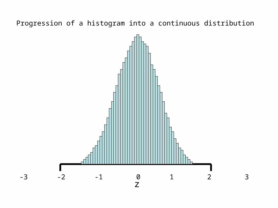
Progression of a histogram into a continuous distribution

-4 -3 -2 -1 0 1 2 3 4

z

Progression of a histogram into a continuous distribution

-4 -3 -2 -1 0 1 2 3 4

z

Progression of a histogram into a continuous distribution

-4 -3 -2 -1 0 1 2 3 4z

Progression of a histogram into a continuous distribution

-4 -3 -2 -1 0 1 2 3 4z

Progression of a histogram into a continuous distribution

-4 -3 -2 -1 0 1 2 3 4z

Progression of a histogram into a continuous distribution

-4 -3 -2 -1 0 1 2 3 4z

Progression of a histogram into a continuous distribution

-4 -3 -2 -1 0 1 2 3 4z

0.4

0.3

0.2

0.1

0.0

Area under the curve

-4 -3 -2 -1 0 1 2 3 4

0.4

0.3

0.2

0.1

0.0

= 50%

50%

Areas under the curve relating to z scores

-4 -3 -2 -1 0 1 2 3 4

0.4

0.3

0.2

0.1

0.0

34.1%

0 to -1

34.1%

0 to +1

Areas under the curve relating to z scores

-4 -3 -2 -1 0 1 2 3 4

0.4

0.3

0.2

0.1

0.0

68.2%

-1 to -2 +1 to +2

13.6% 13.6%

Central limit theorem

• In reasonably large samples (25 or more) the distribution of the means of many samples is normal even though the data in individual samples may have skewness, kurtosis or unevenness.

• Therefore, a t-test may be computed on almost any set of continuous data, if the observations can be considered random and the sample size is reasonably large.

Areas under the curve relating to z scores

-4 -3 -2 -1 0 1 2 3 4

0.4

0.3

0.2

0.1

0.0

68.2% 13.6% 13.6%95.4%

Areas under the curve relating to z scores

-4 -3 -2 -1 0 1 2 3 4

0.4

0.3

0.2

0.1

0.0

95.4%2.1% 2.1%

-2 to -3 +2 to +3

Areas under the curve relating to z scores

-4 -3 -2 -1 0 1 2 3 4

0.4

0.3

0.2

0.1

0.0

99.6%

Areas under the curve relating to +z scores (one tailed tests)

-4 -3 -2 -1 0 1 2 3 4

0.4

0.3

0.2

0.1

0.0

84.1%

Acceptance area

Critical area =15.9%

Areas under the curve relating to +z scores (one tailed tests)

-4 -3 -2 -1 0 1 2 3 4

0.4

0.3

0.2

0.1

0.0

97.7%

Acceptance area

Critical area =2.3%

Areas under the curve relating to +z scores (one tailed tests)

-4 -3 -2 -1 0 1 2 3 4

0.4

0.3

0.2

0.1

0.0

99.8%

Acceptance area

Critical area =0.2%

Asymmetric Distributions

-4 -3 -2 -1 0 1 2 3 4

Positively Skewed RightNegatively Skewed Left

Distributions (Kurtosis)

-4 -3 -2 -1 0 1 2 3 4

Flat curve =Higher level of deviation from the mean

High curve =Smaller deviation from the mean

Distributions (Bimodal Curve)

-4 -3 -2 -1 0 1 2 3 4

-3 -2 - + +2 +3-3 -3 -2 -2 -1-1 00 11 22 33

Z scores

Theoretical normal distribution with standard deviations

Probability [% of area in the tail(s)]Upper tail .1587 .02288 .0013Two-tailed .3173 .0455 .0027

What is the z score for 0.05 probability? (one-tailed test)1.645

What is the z score for 0.05 probability? (two tailed test) 1.96

What is the z score for 0.01? (one-tail test)2.326

What is the z score for 0.01 probability? (two tailed test)

2.576

The Relationship Between Z and X

55 70 85 100 115 130 145

-3 -2 -1 0 1 2 3

P(X)<130

x

Z

=100

=15

X=

Z=

Population MeanPopulation Mean

Standard DeviationStandard Deviation

130 – 100 15

2

Central limit theorem

• In reasonably large samples (25 or more) the distribution of the means of many samples is normal even though the data in individual samples may have skewness, kurtosis or unevenness.

• Therefore, a t-test may be computed on almost any set of continuous data, if the observations can be considered random and the sample size is reasonably large.

(x - x)2

n - 1s =

Student’s t distribution

t =x -

s / n

Standard deviation

Standard Error of the Mean

SE = s/ N

68 7276 7685 8587 879093 93 9494959798 98 103 103105 105105 105107 114117 117118 118119 119123 123124127 127151 151159217 217

N = 15

X = 114.9

s = 34.1

sx = 8.8

Sample

SE = 34.1/ 15

SE = 34.1/ 3.87

SE = 34.1/ 15

SE = 8.8

= 109.2 = 30.2

Confidence Intervals

• The sample mean is a point estimate of the population mean. With the additional information provided by the standard error of the mean, we can estimate the limits (interval) within which the true population mean probably lies.

Source: Osborn

Confidence Intervals

• This is called the confidence interval which gives a range of values that might reasonably contain the true population mean

• The confidence interval is represented as: a b– with a certain degree of confidence - usually

95% or 99% Source: Osborn

Confidence Intervals• Before calculating the range of the interval, one

must specify the desired probability that the interval will include the unknown population parameter - usually 95% or 99%.

• After determining the values for a and b, probability becomes confidence. The process has generated an interval that either does or does not contain the unknown population parameter; this is a confidence interval.

Source: Osborn

Confidence Intervals

• To calculate the Confidence Interval (CI)

)/( nsXCI

Source: Osborn

Confidence Intervals

• In the formula, is equal to 1.96 or 2.58 (from the standard normal distribution) depending on the level of confidence required:– CI95, = 1.96

– CI99, = 2.58Source: Osborn

Confidence Intervals• Given a mean of 114.9 and a standard

error of 8.8, the CI95 is calculated:

= 114.9 + 17.248

= 97.7, 132.1Source: Osborn

)8.8(96.19.114

)/(95

nsXCI