Higher symmetry and gapped phases of gaugetheories

Anton KapustinCalifornia Institute of Technology, Pasadena, CA

Ryan ThorngrenUniversity of California, Berkeley, CA

August 23, 2016

Abstract

We study topological field theory describing gapped phases of gaugetheories where the gauge symmetry is partially Higgsed and partiallyconfined. The TQFT can be formulated both in the continuum andon the lattice and generalizes Dijkgraaf-Witten theory by replacing afinite group by a finite 2-group. The basic field in this TQFT is a2-connection on a principal 2-bundle. We classify topological actionsfor such theories as well as loop and surface observables. When thetopological action is trivial, the TQFT is related to a Dijkgraaf-Wittentheory by electric-magnetic duality, but in general it is distinct. Wepropose the existence of new phases of matter protected by highersymmetry.

1 Introduction and summary

Gapped phases of matter are described at long distances by unitaryTopological Quantum Field Theories. Thus it is of great interest totry to classify unitary TQFTs, at least in space-time dimensions upto four. Since gauge interactions are ubiquitous in nature, it is par-ticularly interesting to identify TQFTs which describe gapped phasesof gauge theories. In the case when the microscopic gauge group is

1

Higgsed down to a finite group G, a complete classification (at leastif no further global symmetries are postulated) has been given by Di-jkgraaf and Witten [1]. Namely, topological actions in d dimensionsare classified by degree-d cohomology classes for G with coefficients inU(1). But DW theories do not exhaust all possibilities. For example,in 3d there are Chern-Simons theories, which are more general than3d DW theories. In this paper we study another class of TQFTs whichexist in all dimensions and are more general than DW theories. TheseTQFTs involve both 1-form and 2-form gauge fields, as well as 0-formand 1-form gauge symmetries. 1-form gauge fields take values in theLie algebra of a Lie group G, while 2-form fields take values in the Liealgebra of another Lie group H. There is a homomorphism t from Hto G and an action α of G on H which enable one to write down aconsistent set of transformation rules. The quadruple G = (G,H, t, α)is what is known as a 2-group (see the next section). It has been ar-gued in [2] that such TQFTs describe massive phases of gauge theorieswhere the microscopic gauge group is partially confined and partiallyHiggsed. More precisely, G is the part of the microscopic gauge groupwhich is not Higgsed, and the image of t is the the confined subgroupof G. In this paper we analyze such TQFTs along the lines of [1].

In the case when H is trivial, our TQFT reduces to a DW theory.The other extreme is when H = G and t is a surjection. In thiscase the whole gauge group is confined, but the theory may have anontrivial “magnetic gauge group” given by ker t. Such theories havebeen recently analyzed in [3, 4] (see also [5] and section 5 of [6]) . Thepresent paper generalizes both [1] and [3, 4].

Here is a brief summary of our results. We show that TQFTswhich describe phases with both Higgs effect and confinement dependon the following data: a finite (possibly non-Abelian) group Π1, a fi-nite abelian group Π2, an action of Π1 on Π2, and a degree-3 groupcohomology class for Π1 with coefficients in Π2. Here Π1 is interpretedas the low-energy “electric” gauge group while Π2 is the “magnetic”gauge group. For every such quadruple and every d > 1 we con-struct a lattice model in d dimensions generalizing the DW model.It describes a lattice gauge field with gauge group Π1 coupled to alattice 2-form with values in Π2. We classify possible action for suchmodels in dimensions 2, 3 and 4. In dimension 2 the theory is equiva-lent to the DW theory for Π1. In dimension 3 the action depends ontwo parameters: a degree-3 cohomology class for Π1 with coefficientsin U(1) and a degree-1 cohomology class for Π1 with coefficients in

2

Π2 = Hom(Π1, U(1)). In dimension 4 the action depends on threeparameters: a degree-4 cohomology class for Π1 with coefficients inU(1), a degree-2 cohomology class for Π1 with coefficients in Π2, anda quadratic function on Π2 with values in U(1). We show that indimension 3 the lattice 2-form can be dualized to a lattice scalar withvalues in Π2. In dimension 4 the lattice 2-form can be dualized toa lattice gauge field provided only the first two terms in the actionare nonzero. We also classify TQFT observables, including surfaceobservables measuring the flux of the 2-form.

Recently DW theories found a new application: it has been arguedthat topological actions for a DW theory with gauge group G classifygapped phases of matter with global symmetry G and no long-rangeentanglement [7, 8, 9]. Such gapped phases are called symmetry-protected phases. We propose that there are more general phaseswhich are protected not by a symmetry group, but by a symmetry2-group. While an ultralocal internal symmetry group acts on de-grees of freedom living on sites of a lattice, a ultralocal 2-symmetryacts on both site and link variables. The groups Π1 and Π2 describesymmetry transformations which live on sites and links, respectively.Gapped phases protected by a 2-group symmetry G are classified bytopological actions for a TQFT based on G. In the special case whenonly the magnetic gauge group Π2 is nontrivial (the case consideredin detail in [3]) it appears that the 2-group TQFT is equivalent to aspecial case of the Walker-Wang TQFT [10, 11].

More generally, as explained below, in d space-time dimensions onecan contemplate symmetry p-groups with p ≤ d, and accordingly onecan have gapped phases with short-range entanglement protected bysuch higher symmetry.

A.K. would like to thank Dan Freed, Sergei Gukov, Michael Hop-kins, Nathan Seiberg, Yuji Tachikawa, and Constantin Teleman fordiscussions. R.T. would like to thank Scott Carnahan, Curt von Key-serlingk, Evan Jenkins, Alex Rasmussen, David Roberts, and UrsSchreiber for discussions. This work was supported in part by theDOE grant DE-FG02-92ER40701 and by the National Science Foun-dation under Grant No. PHYS-1066293 and the hospitality of theAspen Center for Physics.

3

2 2-groups

We begin by recalling the notion of a 2-group [12] and its physicalinterpretation [2]. The most concise definition uses the language ofhigher categories. A (weak) 2-group is a weak 2-category with a singleobject and such that all 1-morphisms are weakly-invertible and 2-morphisms are invertible. This is analogous to the definition of agroup as a category with a single object and such that all morphismsare invertible.

The most pedestrian definition goes as follows. A 2-group is aquadruple G = (G,H, t, α) where G and H are groups, t : H→G isa group homomorphism, and α : G→Aut(H) is an action of G on Hsuch that the following two identities hold:

t(α(g)(h)) = gt(h)g−1, α(t(h))(h′) = hh′h−1. (1)

A 2-group defined in this way is also known as a crossed module.The relation between the two definitions is this: G is the set of 1-morphisms, H is the set of 2-morphisms from the identity 1-morphismto all other 1-morphisms, the map t assigns to a 2-morphism its target1-morphism.

Let us give a few examples of 2-groups. One simple class of ex-amples is obtained by taking G to be a connected simple Lie group,t : H→G to be a covering map, and α to be given by conjugation:h 7→ ghg−1, where g = t−1g. Note that while t−1 is multivalued, dif-ferent choices are different only by elements of the center of H, andtherefore α is well-defined. A nontrivial finite example is provided byH = G = Z4, t(n) = 2n, and α(n)(m) = (−1)nm.

We are interested in the case when G and H are Lie groups, andthe maps t and α are smooth; such a 2-group is called a Lie 2-group.The physical meaning of these data is as follows: G is the subgroup ofthe microscopic gauge group which is not broken by the Higgs effect,im t ⊂ G is the part of G which is confined due to monopole conden-sation (this subgroup is normal, as a consequences of the identities(1), coker t = G/im t is the low-energy gauge group, ker t is the groupwhose elements label conserved magnetic fluxes (it is a subgroup ofthe center of H; we will call it the magnetic gauge group). In theabove finite example, the unbroken gauge group is Z4, its Z2 sub-group is confined, so the low-energy electric gauge group is Z2. Themagnetic gauge group is also Z2, and the electric gauge group acts onthe magnetic fluxes by “charge conjugation”.

4

For groups we have an obvious notion of an isomorphism; for 2-groups a better notion is that of equivalence (of 2-categories). Thisnotion does not preserve the sets G and H, it only preserves the setscoker t and ker t. This is very reasonable from the physical point ofview: representations of coker t describe electric sources visible at longdistances, elements of ker t describe magnetic sources, but G and Hthemselves are not observable at long distances. We will see that forany 2-group G there is a TQFT which depends only on the equivalenceclass of G.

It is thus natural to ask what sort of data describe the equivalenceclass of a 2-group. It turns out it is a quadruple (Π1,Π2, α, β), whereΠ1 = coker t is a group, Π2 = ker t is an abelian group, α is an actionof Π1 on Π2 (it descends from the action of G on H, so we denoteit by the same letter), and β is an element of H3(BΠ1,Π2). Hereand below BG denotes the classifying space of principal G-bundles. Ifthe group G is finite, it is defined up to homotopy by the conditionπn(BG) = 0 for n > 1 and π1(BG) = G [13]. By definition, there is aprincipal G-bundle EG with base BG such that the total space of EGis contractible. Group cohomology of G is defined in terms of EG.Namely, if G acts on an abelian group M , we have an associated flatbundle over BG with fiber M , and Hd(BG,M) denotes the degree-dcohomology of BG with coefficients in this bundle.

The definition of α : Π1→Aut(Π2) should be clear: one first checksthat the action of G on H maps ker t to itself, and then that elementsof im t act trivially on ker t. This implies that coker t acts on ker t.Physically, this is also quite natural: the residual gauge group mayact on the magnetic flux, like in the case of the gauge group O(2n),where charge conjugation is part of the gauge group and flips the signof the magnetic flux.

The definition of β is less obvious. Mathematically, one uses thefact [14] that elements of H3(BΠ1,Π2) can be interpreted as equiva-lence classes of double extensions of Π1 by Π2, with a fixed action ofΠ1 on Π2. That is, these are equivalence classes of four-term exactsequences

1→Π2→H ′→G′→Π1→1,

where (G′, H ′, t′, α′) is a crossed module with coker t′ = Π1, ker t′ =Π2, and with α′ inducing our chosen action of Π1 on Π2. To get β wesimply take the tautological sequence

1→ker t→H→G→coker t→1

5

We will see that the TQFT depends on (Π1,Π2, α, β) and nothing else.However, the continuum action is more conveniently written using thedata (G,H, t, α). This is because we normally assume that Π1 andΠ2 are finite (to ensure that the low-energy theory is gapped), butto write down a continuum action it is convenient to work with fieldswhich take values in the Lie algebras of G and H.

The most basic example of a group arising from topology is thefundamental group of a (pointed connected) topological space. Thisgroup encodes the homotopy 1-type of a space. Similarly, there is a 2-group associated to any pointed connected topological space whichencodes its homotopy 2-type. This 2-group has G = π1(X1, x0),H = π2(X,X1, x0), where X1 is a 1-skeleton of X, and x0 is themarked point. We will call it the fundamental 2-group of X. Thehomotopy equivalence class of these data is encoded by the quadruple(π1(X,x0), π2(X,x0), α, β), where α is the usual monodromy action ofπ1 on π2 and β ∈ H3(Bπ1, π2) is the so-called Postnikov invariant ofX.

3 2-gauge theory in the continuum

The path-integral of the DW theory is constructed as an integral overthe moduli space of flat connections with a structure group G. Sim-ilarly, we can construct a TQFT whose path-integral is an integralover the moduli space of flat 2-connections with a structure 2-groupG. But first we need to define the notion of a flat 2-connection on amanifold X.

A flat connection for a group G can be defined as a homomorphismfrom π1(X) to G. Similarly, a flat 2-connection for a 2-group G can bedefined as a “2-homomorphism” from the fundamental 2-group of Xto G. However, both of these definitions are not manifestly local andtherefore not suitable for constructing a TQFT . A local definition ofa flat 2-connection goes as follows [16, 17].

Let g, h be the Lie algebras of G and H. Let t : h→g be thehomomorphism of Lie algebras induced by the homomorphism of Liegroups t : H→G. Since ker t and coker t were assumed to be finite, t isan isomorphism. Let α : G→Aut(h) be the action of G on h inducedby α. Let {Ui}, i ∈ I, be a cover of X such that all overlaps arecontractible. A flat 2-connection with structure 2-group G is definedby the following data. On each chart Ui one has a g-valued 1-form Ai,

6

on each Uij one has a G-valued function gij and an h-valued 1-formλij , and on each Uijk one has an H-valued function hijk so that thefollowing conditions are satisfied:

• On each Uij one has Aj = gijAig−1ij + gijdg

−1ij − t(λij).

• On each Uijk one has gik = t(hijk)gjkgij , and

h−1ijkλikhijk = α(gjk)(λij) + λjk − h−1

ijkdhijk

−h−1ijk t

−1(Ak)hijk + t−1(Ak) .

• On each Uijkl one has hijlhjkl = hikl · α(gkl)(hijk).

We can also introduce h-valued 2-forms Bi on each Ui by Bi = t−1FAi ,where f1 = dA+A∧A. Alternatively, we can treat them as indepen-dent 2-forms, with suitable gluing conditions on double overlaps, andregard the condition FAi = t(Bi) as an equation of motion.

Just like in the case of ordinary connections, there is a notionof gauge equivalence of flat 2-connections. Let (Ai, gij , λij , hijk) and(A′i, g

′ij , λ

′ij , h

′ijk) be a pair of 2-connections. A gauge-equivalence be-

tween them is a G-valued function gi and an h-valued 1-form λi oneach Ui, together with an H-valued function hij on every Uij such that

• On each Ui one has

A′i = giAig−1i + gidg

−1i − t(λi).

• On each Uij one has g′ij = t(hij)gjgijg−1i , and

λ′ij = hij (α(gj)(λij) + λj)h−1ij − α(g′ij)(λi)

+hijdh−1ij + hij t

−1(A′j)h−1ij − t

−1(A′j) .

• On each Uijk one has

h′ijk = hikα(gk)(hijk)h−1jk α(g′jk)(h

−1ij ).

There are also 2-gauge transformations between gauge transforma-tions, see [16, 17, 2] for details.

If 2-forms Bi are regarded as independent variables, then the actionin d space-time dimensions has the form

S =∫〈(f1 − t(B)),∧b〉+ Stop,

7

where b is a Lagrange multiple (d− 2)-form with values in g∗ and Stopis a topological action which is invariant under gauge equivalence offlat 2-connections. If we regard Bi as dependent variables, then theaction contains only Stop. Below we will determine the most generalform of Stop in dimension 4 and lower.

For now, let us show that the moduli space of flat 2-connections canbe reformulated purely in terms of the data (Π1,Π2, α, β). First, weuse the 1-form gauge transformations to set Ai = 0 (and consequentlyBi = 0). This ensures that the 1-forms λij is pure gauge:

λij = t−1(gijdg−1ij ),

and simultaneously that for any two points p, p′ ∈ Uij we have

g−1ij (p)gij(p′) ∈ im t.

Thus if we project gij to Π1 = coker t, the resulting Π1-valued functionis constant. We denote this function aij .

Next, let us choose a map s : Π1→G which is an inverse of theprojection G→Π1. In general, we cannot choose s to be a homomor-phism, but we can always choose it so that s(x)−1 = s(x−1) for allx ∈ Π1. By definition, s(aij)g−1

ij is a function on Uij which takesvalues in im t. Thus there exists an H-valued function hij such thatt(hij) = s(aij)g−1

ij . Performing another gauge transformation, nowwith λi = 0, gi = 1 and hij chosen as above, we bring the data defin-ing a 2-connection to the form

Ai = 0, λij = 0, gij = s(aij).

In addition, the functions hijk : Uijk→H are now constant. Thus theequivalence class of the flat 2-connection is completely determined bythe constant functions aij : Uij→Π1 and hijk : Uijk→H. On everyUijk these functions satisfy a constraint:

t(hijk) = s(aik)s(aji)s(akj),

which implies that the functions a form a Cech 1-cocycle with valuesin Π1:

aikajiakj = 1.

Furthermore, hijk can be expressed in terms of the functions a and aconstant function bijk : Uijk→Π2:

hijk = bijkf(aik, aji),

8

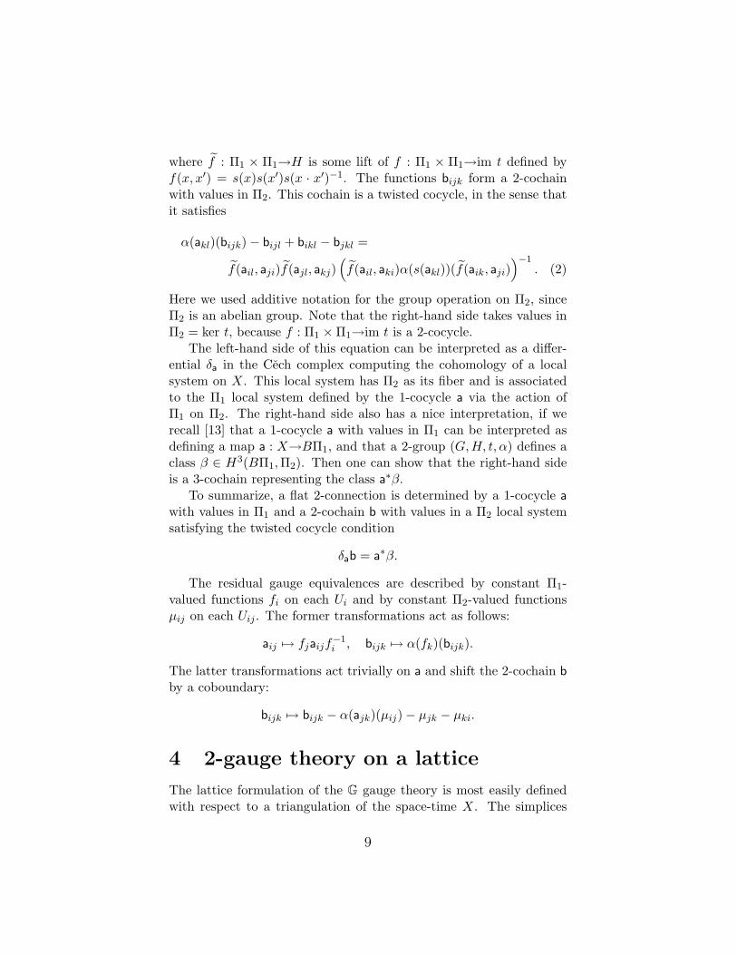
where f : Π1 × Π1→H is some lift of f : Π1 × Π1→im t defined byf(x, x′) = s(x)s(x′)s(x · x′)−1. The functions bijk form a 2-cochainwith values in Π2. This cochain is a twisted cocycle, in the sense thatit satisfies

α(akl)(bijk)− bijl + bikl − bjkl =

f(ail, aji)f(ajl, akj)(f(ail, aki)α(s(akl))(f(aik, aji)

)−1. (2)

Here we used additive notation for the group operation on Π2, sinceΠ2 is an abelian group. Note that the right-hand side takes values inΠ2 = ker t, because f : Π1 ×Π1→im t is a 2-cocycle.

The left-hand side of this equation can be interpreted as a differ-ential δa in the Cech complex computing the cohomology of a localsystem on X. This local system has Π2 as its fiber and is associatedto the Π1 local system defined by the 1-cocycle a via the action ofΠ1 on Π2. The right-hand side also has a nice interpretation, if werecall [13] that a 1-cocycle a with values in Π1 can be interpreted asdefining a map a : X→BΠ1, and that a 2-group (G,H, t, α) defines aclass β ∈ H3(BΠ1,Π2). Then one can show that the right-hand sideis a 3-cochain representing the class a∗β.

To summarize, a flat 2-connection is determined by a 1-cocycle awith values in Π1 and a 2-cochain b with values in a Π2 local systemsatisfying the twisted cocycle condition

δab = a∗β.

The residual gauge equivalences are described by constant Π1-valued functions fi on each Ui and by constant Π2-valued functionsµij on each Uij . The former transformations act as follows:

aij 7→ fjaijf−1i , bijk 7→ α(fk)(bijk).

The latter transformations act trivially on a and shift the 2-cochain bby a coboundary:

bijk 7→ bijk − α(ajk)(µij)− µjk − µki.

4 2-gauge theory on a lattice

The lattice formulation of the G gauge theory is most easily definedwith respect to a triangulation of the space-time X. The simplices

9

need to be oriented so that our formulas have the proper signs. Thiscan be achieved by ordering the vertices. We use the convention thathigher vertex labels point towards lower vertex labels since our groupelements act on the left. This is demonstrated in figures below. Thetheory depends on neither the triangulation nor this ordering.

To get a lattice description of the G gauge theory we use the de-scription of flat 2-connections in terms of the data (Π1,Π2, α, β) ob-tained in the previous section. All one has to do is to rewrite thecochains a and b and conditions on them in simplicial terms. Sincethis is standard, we simply state the results.

A field configuration is an assignment of an element of A ∈ Π1

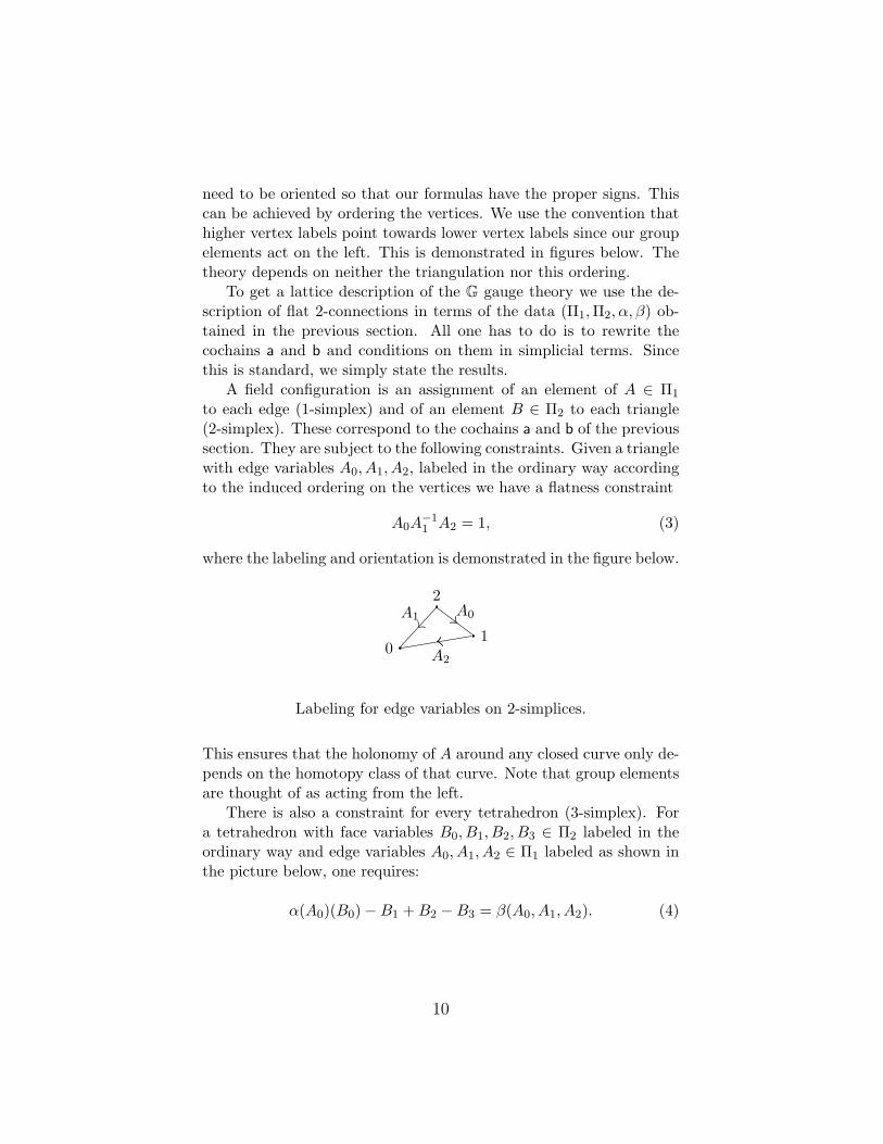
to each edge (1-simplex) and of an element B ∈ Π2 to each triangle(2-simplex). These correspond to the cochains a and b of the previoussection. They are subject to the following constraints. Given a trianglewith edge variables A0, A1, A2, labeled in the ordinary way accordingto the induced ordering on the vertices we have a flatness constraint

A0A−11 A2 = 1, (3)

where the labeling and orientation is demonstrated in the figure below.

10

2A0A1

A2

Labeling for edge variables on 2-simplices.

This ensures that the holonomy of A around any closed curve only de-pends on the homotopy class of that curve. Note that group elementsare thought of as acting from the left.

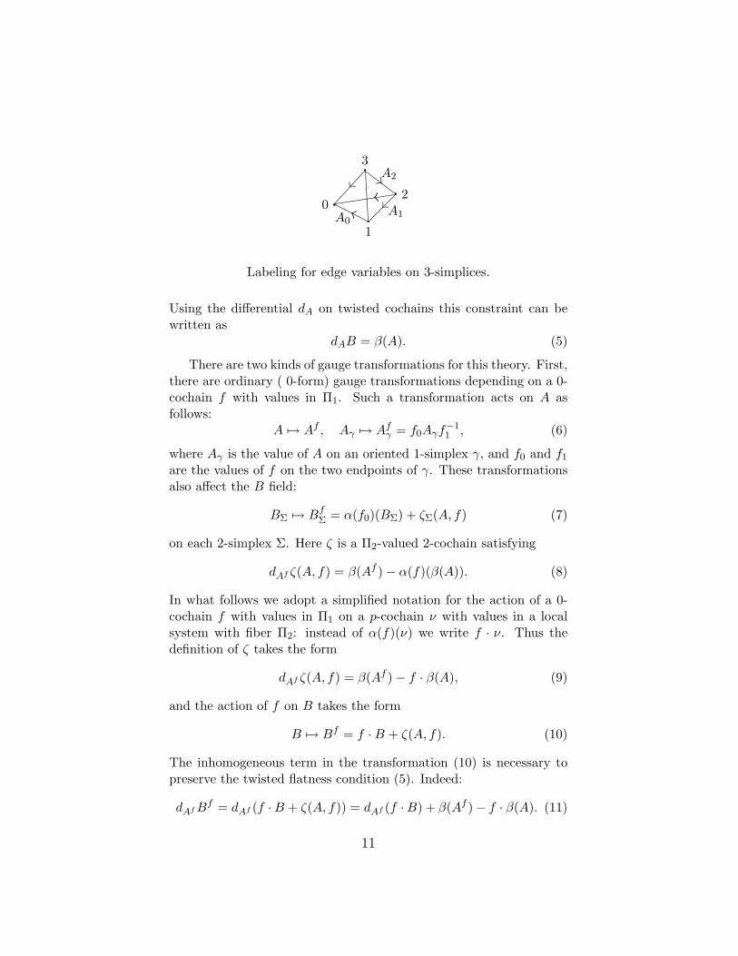
There is also a constraint for every tetrahedron (3-simplex). Fora tetrahedron with face variables B0, B1, B2, B3 ∈ Π2 labeled in theordinary way and edge variables A0, A1, A2 ∈ Π1 labeled as shown inthe picture below, one requires:

α(A0)(B0)−B1 +B2 −B3 = β(A0, A1, A2). (4)

10

1

20

3

A1A0

A2

Labeling for edge variables on 3-simplices.

Using the differential dA on twisted cochains this constraint can bewritten as

dAB = β(A). (5)

There are two kinds of gauge transformations for this theory. First,there are ordinary ( 0-form) gauge transformations depending on a 0-cochain f with values in Π1. Such a transformation acts on A asfollows:

A 7→ Af , Aγ 7→ Afγ = f0Aγf−11 , (6)

where Aγ is the value of A on an oriented 1-simplex γ, and f0 and f1

are the values of f on the two endpoints of γ. These transformationsalso affect the B field:

BΣ 7→ BfΣ = α(f0)(BΣ) + ζΣ(A, f) (7)

on each 2-simplex Σ. Here ζ is a Π2-valued 2-cochain satisfying

dAf ζ(A, f) = β(Af )− α(f)(β(A)). (8)

In what follows we adopt a simplified notation for the action of a 0-cochain f with values in Π1 on a p-cochain ν with values in a localsystem with fiber Π2: instead of α(f)(ν) we write f · ν. Thus thedefinition of ζ takes the form

dAf ζ(A, f) = β(Af )− f · β(A), (9)

and the action of f on B takes the form

B 7→ Bf = f ·B + ζ(A, f). (10)

The inhomogeneous term in the transformation (10) is necessary topreserve the twisted flatness condition (5). Indeed:

dAfBf = dAf (f ·B + ζ(A, f)) = dAf (f ·B) + β(Af )− f · β(A). (11)

11

A simple calculation shows

dAf (f ·B) = f · dAB = f · β(A),

hence the pair (Bf , Af ) satisfies the condition (5).Note that the equation (9) for ζ always has a solution, since the

cohomology class of β(A) does not change when one replaces A by agauge-equivalent one (this follows from the fact that β is closed). Wecan even choose ζ to satisfy the normalization condition

ζ(1g, f) = 0, (12)

for all constant f ∈ Π1 and gauge-trivial A = 1g. This normalizationis possible since if f is constant, the cochain β can be normalized sothat β(1gf ) = f · β(1g).

The second class of gauge transformations are 1-form gauge trans-formations depending on a 1-cochain a with values in Π2. These trans-formations do not affect the 1-cocycle A, whileB transforms as follows:

BΣ 7→ BaΣ = BΣ + α(A2)(a0)− a1 + a2, (13)

for every 2-simplex Σ whose boundary ∂Σ is assigned a0, a1, a2. Inother words, B 7→ Ba = B+ dAa. These transformations preserve thetwisted flatness constraint for B since d2

A = 0.The 1-form gauge transformations have 2-gauge transformations

parametrized by an assignment of an element of Π2 to each vertexunder which the 1-form gauge parameters a transform as

agγ = aγ + g1 − α(Aγ)(g0), (14)

where ∂γ is assigned g0, g1. One can check that two 1-form gaugetransformations related by such a 2-gauge transformation act identi-cally on the fields.

1-form and 0-form gauge transformations do not commute in gen-eral. Let a be a 1-cochain with values in the Π2 local system associatedto a Π1 local system, and f be a 0-cochain with values in Π1. Let usdenote by (a, f) as a 1-form transformation with a parameter a fol-lowed by a 0-form transformation with a parameter f . Then

(a, f) = (0, f) ◦ (a, 1) = (f · a, 1) ◦ (0, f). (15)

For future use, we record the transformations of B and A under ageneral transformation (a, f):

Ba,f = f · (B + dAa) + ζ(A, f), (16)

12

andAa,f = Af . (17)

When composing two gauge transformations, where the first oneis (a1, f1), it is often convenient to write the second one as (f1 · a2, f2)rather than (a2, f2). We will use this convention below.

The reader might have noticed the similarity between β and ζ onone hand, and the Chern-Simons form and its descendant on the otherhand. This is not a coincidence, since the Chern-Simons form for acompact Lie group G can be regarded as a 3-cocycle on the classifyingspace of flat G-connections [18]. In superstring theory and super-gravity, the Chern-Simons form modifies the definition of the gauge-invariant field-strength of a 2-form gauge field B, while the descendantof the Chern-Simons form describes how the B-field transforms underordinary gauge symmetries [19]. This is clearly analogous to how βmodifies the flatness constraint on B (eq. (5)) and how ζ enters thetransformation law for B (eq. (7)).

It is well-known that the descent procedure can be continued, sothat from the 2-cochain ζ(A, f) one gets a 1-cochain κ(A, f, g), etc.Below we will need the definition of κ only for A = 0, so let us describehow it is constructed. By definition,

β(Ag)− g · β(A) = dAgζ(A, g),

where A is an arbitrary 1-cochain with values in Π1 and g is an arbi-trary 0-cochain with values in Π1. Let us set A = 1f , where f is anarbitrary 0-cochain with values in Π1 (i.e. we let A be cohomologousto the trivial 1-cochain). Then we get

β(1gf )− g · β(1f ) = d1gf ζ(1f , g) = gf · d(

(gf)−1 · ζ(1f , g)).

This equation implies that the 2-cochain

(gf)−1 · ζ(1, gf)− f−1 · ζ(1, f)− (gf)−1 · ζ(1f , g)

is closed for any 0-cochains f and g. Contractibility of EG impliesthat this cochain is exact, i.e. there exists a 1-cochain κ(g, f) withvalues in Π2 such that

(gf)dκ(g, f) = g · κ(1, f) + ζ(1f , g)− ζ(1, gf). (18)

This 1-cochain κ is the second descendant of β.

13

The partition function is defined as the weighted sum over allallowed field configurations, divided by the order of the group ofgauge transformations and multiplied by the order of the group of2-gauge transformations. The weight must be gauge-invariant andtopologically-invariant, in the sense that the partition function mustbe invariant under a subdivision of the triangulation. The most gen-eral weight function satisfying these conditions will be described insection 6.

5 Loop and surface observables

The above construction of the 2-group TQFT works in arbitrary space-time dimension (and gives something different from the Dijkgraaf-Witten theory in dimension 3 or higher). We now discuss observablesin this TQFT focusing on the 4d case.

The 2-group TQFT in 4d describes the phase with both electricgauge group Π1 and magnetic gauge group Π2 and therefore admitstwo types of loop observables and two types of surface observables.Let us begin with loop observables. There are ordinary Wilson loopsfor the lattice gauge field A; they are labeled by representations of Π1.There are also disorder loop operators which correspond to ’t Hooftloops in the microscopic gauge theory. In the lattice formulation, onechooses a closed path γ on the dual cell complex and modifies thetwisted cocycle condition (4) on every 3-simplex Tl dual to an edge ofl ∈ γ as follows:

α(A0)(B0)−B1 +B2 −B3 = β(A0, A1, A2) +Hl.

Here Hl is an element of Π2. One can think of the elements Hl asdefining a dual 1-cochain with values in a Π2 local system on the loopγ. The above equation implies that this cochain is a cocycle, so theelements Hl for different l all lie in the same orbit of the Π1 action onΠ2. Therefore ’t Hooft loops are labeled by orbits of the Π1-action inΠ2.

There are also order and disorder surface observables. Disordersurface observables are defined by the condition that the Π1 gaugefield has a fixed holonomy along a loop linking a homologically triv-ial surface Σ. In the lattice formulation, Σ should be thought of ascomposed of 2-cells of the dual cell complex, and the insertion of thedisorder operator supported on Σ amounts to deforming the 1-cocycle

14

condition on A for every 2-simplex dual to the 2-cells of Σ. Suchsurface observables are labeled by conjugacy classes in Π1.

There are also Wilson surface observables are labeled by elementsof Π2 = Hom(Π2, U(1)) which satisfy two conditions. First of all,η ∈ Π2 must be invariant under the action of Π1. Second, η ◦ β ∈H3(Π1, U(1)) must vanish.

A quick way to see how these two conditions on η arise is as follows.The Wilson surface measures the flux of B though Σ. Thus it mustinvolve a product over all 2-simplices making up Σ, with each simplexcontributing a phase η(±B), where the sign is determined by the mu-tual orientation of Σ and the 2-simplex in question. Invariance withrespect to gauge transformations requires η to Π1-invariant, givingthe first condition on η. To obtain the second condition, note that theWilson surface observable should evaluate to 1 if Σ is the boundaryof a 3-simplex and no ’t Hooft loop intersects this 3-simplex. Apply-ing η to the twisted cocycle condition (4) we see that this is true ifη ◦ β(A0, A1, A2) = 0 for all A0, A1, A2 ∈ Π1. More generally, supposethe 3-cochain η ◦ β(A0, A1, A2) is not zero but is a coboundary of a2-cochain on Π1 with values in U(1):

η ◦ β(A0, A1, A2) = γ(A0, A1A2)γ(A0A1, A2)−1γ(A1, A2)γ(A0, A1)−1.

Then one can modify the definition of the Wilson surface observable bymultiplying the weight assigned to a 2-simplex by a factor γ(A0, A1).The modified observable is trivial on an elementary 3-simplex, as re-quired. On the other hand, if η ◦ β is not cohomologous to zero, nolocal modification of the weight can solve the problem.

Apart from the surface observables measuring the flux of B, onecan also construct surface observables which are sensitive only to the1-cocycle A. Namely, if we restrict A to a closed surface Σ, it definesa principal G-bundle on Σ with structure group Π1, and any class inH2(BΠ1, U(1)) gives a surface observable. Such observables are trivialif Σ is simply-connected, but are nontrivial in general.

The most general observable supported on a surface Σ involvesboth the B fluxes and the A-holonomies along a marked 1-skeleton ofΣ. The Π1 invariance of such operators may rely on the transformationof both A and B variables, so they are not necessarily products ofWilson lines and Wilson surfaces.

In three dimensions the analysis is very similar, so we just presentthe results. There are local operators (i.e. operators supported atpoints) labeled by orbits of Π1 action on Π2. These correspond to ’t

15

Hooft point operators in the microscopic gauge theory. There are twokinds of loop observables: Wilson loops labeled by representations ofΠ1 and vortex loops labeled by conjugacy classes in Π1. Finally thereare Wilson surfaces defined in the same way as in four dimensions.That is, they are labeled by a Π1-invariant element η ∈ Π2 whichannihilates the class β, together with a class in H2(BΠ1, U(1)).

6 Topological actions

As described in the appendix, the configuration data (A,B) are equiv-alent to a simplicial map B from the spacetime X into the classifyingspace BG of the 2-group. Gauge equivalence classes are homotopyclasses of these maps. This is analogous to the fact that a flat G-connection can be viewed as a map to the classifying space BG. Wetherefore define an action functional for a d-dimensional theory bypicking a class L ∈ Hd(BG,R/Z) and setting

S(B) = 2πi∫XB∗L. (19)

This action is gauge invariant and manifestly topological.To calculate the cohomology group Hd(BG,R/Z) we need a good

understanding of the classifying space BG. This space can be taken tobe any space with G as its homotopy type. This implies π1(BG) = Π1,π2(BG) = Π2, and all higher homotopy groups vanish. It also meansthat the action of π1(BG) on π2(BG) is given by α as well as a morecomplicated condition involving the Postnikov invariant β. In theappendix we describe a cell structure for this space.

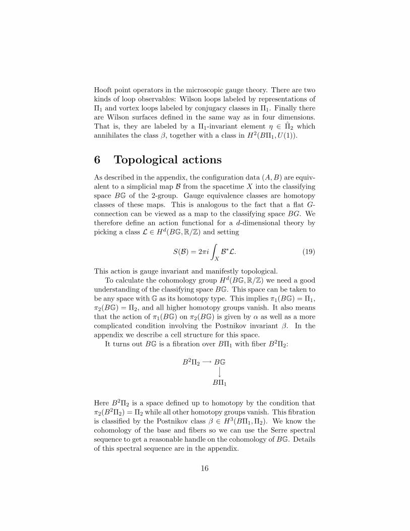
It turns out BG is a fibration over BΠ1 with fiber B2Π2:

BG

BΠ1

B2Π2

Here B2Π2 is a space defined up to homotopy by the condition thatπ2(B2Π2) = Π2 while all other homotopy groups vanish. This fibrationis classified by the Postnikov class β ∈ H3(BΠ1,Π2). We know thecohomology of the base and fibers so we can use the Serre spectralsequence to get a reasonable handle on the cohomology of BG. Detailsof this spectral sequence are in the appendix.

16

The Serre spectral sequence tells us that for 2-dimensional the-ories, L is a sum of two terms. The first term is an element ofH2(B2Π2,R/Z). This cohomology group is isomorphic to the groupΠ2 of homomorphisms Π2 → R/Z. A character η ∈ Π2 gives aclass on BG if and only if it is invariant under the action of Π1 andη(β) ∈ H3(BΠ1,R/Z) is zero as a cohomology class. An interpretationof these conditions was discussed in the previous section.

The second term can be any element ω ∈ H2(BΠ1,R/Z).The most general 2d action is therefore

S(B) = 2πi∫Xη(B) + 2πi

∫XA∗ω,

where here B is the Π2-valued 2-form field and A : X→BΠ1 is thecomposition of the classifying map B : X → BG with the fibrationmap BG→ BΠ1. Equivalently this is the map X → BΠ1 determinedby the A variables. Note that if X = S2, then since π2(BΠ1) = 0, thepullback A∗ω always integrates to zero.

In three dimensions, we also find that L is a sum of two terms.The first term is an element ω ∈ H3(BΠ1,R/Z). The action dependson this element only up to the addition of a term of the form η(β),where η is a Π1-invariant character of Π2.

The second term is an element λ ∈ H1(BΠ1, Π2). As a cochainon BG, λ is closed only if 〈λ,∪β〉 ∈ H4(BΠ1,R/Z) vanishes as acohomology class.

The most general 3d action is therefore

S(B) = 2πi∫XA∗λ ∪B + 2πi

∫XA∗ω.

Here the cup product between A∗λ and B is formed using the pairingbetween Π2, where B takes values, and Π∗2, where λ takes values. Notethat on a simply-connected space ω does not contribute since A∗ω isexact. On the other hand, athough A∗λ is exact, B is not closed, sotheir contraction is not necessarily exact.

In four dimensions the action is a sum of three terms. The firstterm depends on an element of H4(B2Π2,R/Z). This group is isomor-phic to the group of quadratic functions q : Π2 → R/Z as discussed in[3]. In order for this cocycle to extend to BG, it needs to be invariantunder the action of Π1. This is equivalent to the quadratic function qbeing invariant. In order for its extension to be closed, 〈β,−〉q needs

17

to vanish as an element of H3(BΠ1, Π2), where the bracket denotesthe associated bilinear form for q.

The second term depends on an element λ ∈ H2(BΠ1, Π2). Thisgives a cocycle on BG when contracted with the B-field only if 〈λ,∪β〉is zero in H5(BΠ1,R/Z).

The third term is an integral of a pull-back of ω ∈ H4(BΠ1,R/Z).The action only depends on ω up to the addition of something of theform 〈γ,∪β〉 for some γ ∈ H1(BΠ1, Π2).

The most general 4d action is therefore

S(B) = 2πi∫Xq∗(PB) + 2πi

∫XA∗λ,∪B + 2πi

∫XA∗ω,

where PB denotes the Pontryagin square of the B-field, and q∗ is themap from the universal quadratic group Γ(Π2) to R/Z correspondingto q. This term is discussed in detail in [3]. Note that because ofthe Postnikov class β, it is only closed after applying q∗. For simply-connected X, as in the three-dimensional case, ω does not contribute,but λ does.

In the case of Dijkgraaf-Witten theory in dimension d, the topo-logical action depends on a class in Hd(BG,U(1)), and one can givean explicit description of the corresponding cocycle as a function of dvariables living in G. From the mathematical viewpoint, this explicitdescription arises from the standard complex computing the cohomol-ogy of BG, while from the physical viewpoint the cocycle is the weightattached to a d-simplex [1]. Similarly, one can give an explicit descrip-tion of a class in Hd(BG, U(1)) as a function of several variables, someof them living in Π1 and some living in Π2, satisfying a certain condi-tion. This condition can be understood mathematically as a cocyclecondition in a standard complex computing the cohomology of BG.However, even in low degrees the formulas are quite unwieldy. Forthis reason we only state them for d = 2. In this case the cocycle is afunction L on Π1×Π1×Π2 with values in R/Z. The cocycle conditionis

L(A0, A1A2;B2)−L(A0A1, A2;B1)−L(A0, A1;B3)+L(A1, A2;B0) = 0,

where B0 is not independent but is expressed through the variablesA0, A1, A2, B1, B2, B3 by means of (4). 2-cocycles for Π1 can be iden-tified with 2-cocycles for BG which do not depend on the Π2 variable.

A 3-cocycle for a 2-group BG depends on three variables in Π1 andthree variables in Π2. In general, a d-cocycle depends on d variables in

18

Π1 and d(d−1)/2 variables in Π2. They can be thought of as labelingedge and triangles containing a given vertex of a d-simplex.

7 Duality

Since the simplicial B-field takes values in an abelian group Π2, onecould try to dualize it. In dimension d the dual variable should live on(d−3)-cells of the dual cell complex and take values in the Pontryagin-dual group Π2 = Hom(Π2, U(1)). But in general a nontrivial topolog-ical action for B obstructs the dualization procedure. An importantspecial case where the dualization can be performed is when the actionis either independent of B, or depends on it linearly. Let us performthe dualization procedure in various dimensions.

For d = 2 the 2-group TQFT is essentially equivalent to theDijkgraaf-Witten theory with gauge group Π1. First of all, the con-straint (4) is not needed in this case. Second, the class η in the 2d ac-tion must vanish, because otherwise the partition function on S2 van-ishes after one sums over the B-fields, which contradicts the axioms ofTQFT [20]. But then summation over B only produces an inessentialnumerical factor, and the theory is clearly equivalent to the Dikgraaf-Witten theory for Π1 with an action given by ω ∈ H2(BΠ1,R/Z).

For d = 3 the action is always linear in B, as explained in theprevious section. Therefore the dualization is always possible. Weimpose the constraint (4) by means of a Lagrange multiplier field Cwhich lives on dual 0-cells and takes values in Π2. Thus we add to theaction a term

2πi∫X〈C, δAB − β(A)〉

and treat B as an unconstrained 2-cochain with values in Π2. Forsimplicity, let us first assume that Π1 acts trivially on Π2. Then thedifferential δA becomes the usual Cech differential δ, and summingover B produces a constraint

δC = −A∗λ,

where λ ∈ H1(BΠ1, Π2).Since we assumed for now that α is trivial, the group H1(BΠ1, Π2)

is merely the group of homomorphisms from Π1 to Π2. Thus theconstraint on C reads explicitly

C1 − C0 + λ(Al) = 0,

19

where l is a 1-cell of the of the dual cell complex with source andtarget 0 and 1.1 This constraint is gauge-invariant provided we assignto C a nontrivial transformation law under Π1 gauge transformations:

C 7→ C + λ(f),

where f is a 0-cochain with values in Π1 parameterizing a gauge trans-formation. Thus the dual theory is a topological sigma-model withtarget Π2 coupled to a topological 3d gauge theory with gauge groupΠ1. The group Π1 acts on Π2 via the homomorphism λ. The actionof the gauge theory is

S = 2πi∫XA∗ω + 2πi

∫X〈C,A∗β〉.

Note that while the first term is the Dijkgraaf-Witten action of the 3dgauge theory, the second term is of a different nature.

The case of nontrivial α is not very different. The constraint on Cnow reads

δAC + λ(A) = 0.

The transformation law for C is now more complicated:

C 7→ α(f)(C) + λ(f),

where α denotes the action of Π1 on Π2 dual to the action of Π1 onΠ2. The dual theory is again a gauged topological sigma-model withthe same action as above.

For d = 4 we need to assume that the first term in the topologicalaction vanishes (i.e. q = 0). Then the action is again linear in B, andB can be dualized to a 1-cochain C with values in Π2. Performingsummation over B we find a constraint on C which reads

δAC = λ(A),

where λ is a cocycle representing a class in H2(Π1, Π2). We also havethe usual constraint which says that A is a 1-cocycle with values inΠ1. One can show that these two constraints can be interpreted asthe flatness constraint for a gauge field (A,C) taking values in an

1Here we neglected the fact that the field A was originally only defined on the 1-cellsof the original triangulation. In more detail, one needs first to pass from the simplicial 1-cochain A to a Π1 local system onX and then restrict to the 1-cells of the dual cell complex.The first step involves a certain arbitrariness which does not change the conclusions.

20

extension of Π1 by Π2 determined by α and λ. Thus the dual theoryis a topological gauge theory with this extension as the gauge group.The action is necessarily of the DW type and has the form

S = 2πi∫XA∗ω + 2πi

∫X〈C,∪A∗β〉.

Note that even if the original 2-group TQFT had a trivial action (i.e.λ and ω vanish), the dual theory has a nontrivial action which isdetermined by β. On the other hand, the class λ which parameterizedthe action of the original theory enters the dual theory only throughthe structure of the gauge group.

8 Phases protected by higher symme-

try

8.1 SPT phases and TQFT

Recently, the Dijkgraaf-Witten TQFT was used in a novel way, as atool to classify symmetry-protected (SPT) phases without long-rangeentanglement [7, 8, 9]. These are phases of matter which have threeproperties: (1) they are gapped; (2) they have a global symmetrygroup G which acts ultralocally; (3) the TQFT describing the low-energy limit is trivial. Here by an ultralocal action of a global sym-metry we mean that there is a lattice realization of the phase wherethe symmetry transformation only mixes degrees of freedom living ona given vertex (0-cell).

It was proposed in [7] that SPT phases in space-time dimension dwith a finite internal 2 symmetry group G are classified by elements ofHd(BG,U(1)). Let us provide an interpretation of this classificationscheme in TQFT terms (see also [9] for a very similar discussion). Weuse the fact that a lattice system with an ultralocal internal symmetrycan be canonically coupled to a flat gauge field with structure groupG. Indeed, locally any flat G-connection is a pure gauge, i.e. a gaugetransformation of the trivial connection. This gauge transformationis defined up to a constant symmetry transformation in G. Since the

2We will focus on the case of finite internal symmetry, but one can generalize it to thecase when G is a compact Lie group which might involve time-reversal.

21

system is local, the lattice action is a sum over all vertices∑v

Sv(φ),

where each term Sv depends only on the degrees of freedom in theimmediate neighborhood of the vertex. Since the symmetry acts ul-tralocally, each Sv is separately invariant under constant symmetrytransformations. We define the action of the system coupled to a flatbackground gauge field as a sum∑

v

Sv(φg),

where φg is a transformation of the field configuration by a local gaugetransformation g describing the flat connection. Since different choicesof g differ by constant symmetry transformations, this expression iswell-defined and gauge-covariant. Now we can integrate out the mat-ter fields and obtain an effective action for the flat gauge field. Itis necessarily topological and therefore must arise from a class inHd(BG,U(1)).

It is natural to ask whether more general 2-group TQFTs we havestudied here and in [2, 3] are related to new phases of matter notcovered by the group cohomology classification. The role of the sym-metry group G is taken by a 2-group G. In this more general setting,a global symmetry transformation is parameterized by an element ofΠ1 and a flat gauge field with gauge group Π2. The action of G is as-sumed to be ultralocal, in the sense that the system can be canonicallycoupled to a flat 2-connection (A,B) with structure group G. If thesystem is gapped and the ground state has short-range entanglement,one can integrate out the matter fields and obtain a topological actionfor (A,B) which is described by an element of Hd(BG, U(1)).

In the case when Π2 is trivial, this reduces to the group coho-mology classification of SPT phases. The opposite extreme is whenΠ1 is trivial. In this case G is completely determined by an abeliangroup Π2, and phases protected by such a 2-symmetry are labeledby Hd(B2Π2, U(1)). The first nontrivial case is d = 4, where Π2-protected phases are classified by quadratic functions on Π2 with val-ues in U(1). The same data classify pre-modular braided tensor cat-egories whose simple objects are labeled by elements of Π2. Sincepre-modular categories are also used in the construction of Walker-Wang TQFTs [10], it seems likely that 2-group TQFTs with trivial

22

Π1 are a special case of Walker-Wang models. Indeed, it has beenconjectured in [10] (see also [11]) that in the continuum limit Walker-Wang models based on Zn are described by a BF action deformedby a term B ∧ B. This agrees with the continuum description of the2-group TQFT discussed in [2, 3].

A simple example of a system with an ultralocal 2-symmetry isgiven by a Yang-Mills theory with gauge group G where all matterfields transform trivially under the center of G. Then the symmetry2-group has Π1 = 0 and Π2 = Z(G). The system can be “minimallycoupled” to a flat B-field with values in Z(G). Essentially, this meansthat one performs the path-integral over Yang-Mills gauge fields withstructure group G/Z(G) and a fixed ’t Hooft flux described by B.The resulting function of B must be an integral over X of a pull-back of a class in Hd(B2Z(G), U(1)). In the case d = 4, one caninterpret the elements of this group as labeling discrete theta-anglesin the underlying Yang-Mills theory [21, 3].

Even more generally, if one dealing with a gapped phase in space-dimension d, symmetry transformations may live on cells of all dimen-sions up to d. This situation is most natural when the “matter fields”involve gauge fields of all form degrees. The symmetry structure inthis case is described by a d-group, i.e. by a d-category with a singleobject and invertible 1-morphisms, 2-morphisms, etc. SPT phases in ddimensions with symmetry d-group G should be classified by degree-dcohomology of the classifying space of G. This classifying space hashomotopy groups which may be non-vanishing in degrees up to d.

8.2 Boundaries of SPT phases

In the case of an SPT phase protected by a finite symmetry groupG, the nontriviality of the corresponding class in Hd(BG,U(1)) hasinteresting physical consequences for the boundary behavior of thephase [8]: the boundary cannot be gapped without either breakingsymmetry or introducing long-range entanglement. The same appearsto be true in the case of phases protected by a d-group symmetry.Namely, the boundary cannot be gapped by any perturbation whichpreserves G as an ultralocal symmetry and does not create long-rangeentanglement. Indeed, if such a perturbation existed, one could couplethe system to a flat d-connection and integrate out the matter fieldseven in the presence of a nonempty boundary. This should produce atopological action for the flat d-connection which is is gauge-invariant

23

on a d-manifold with a boundary. Such an action should have theform

S = 2πi∫XA∗ω − 2πi

∫∂XA∗ψ

for some ψ ∈ Hd−1(BG,R/Z). But this action is gauge-invariant onlyif ω = δψ, which contradicts the nontriviality of ω ∈ Hd(BG,R/Z).Thus if G is preserved on the boundary, the boundary can be gappedonly at the expense of creating a topological order on the boundary.Moreover, neither the bulk action, nor the boundary TQFT action areseparately gauge-invariant in this case (there is an “anomaly-inflow”from the bulk to the boundary). Thus G is realized anomalously onthe boundary, and this anomaly is measured by ω.

Alternatively, if we insist on having no topological order on theboundary, G must be explicitly or spontaneously broken there, andwe can describe possible patterns of symmetry breaking. Namely, Gmust be broken down to a d-subgroup H such that ω becomes exactwhen restricted to H, ω|H = δψ. Only then is it possible to write agauge-invariant effective action in the presence of a boundary.

8.3 Lattice realization of an SPT phase

As in [7], we can give descriptions of ungauged ground states thatrealize this phase in the “group cohomology” basis. Suppose that G isa 2-group described by a quadruple (Π1,Π2, α, β), as above.3 Let Mdenote the spatial manifold. We will compute the ground state on Mby performing the path integral in the TQFT over a spacetime withboundary M . For example, if M is a sphere, we take our spacetime Bto be a ball. For these theories, spacetime does not need to be smooth,so we can always take spacetime to be CM , the cone over M .

A map from CM to BG is the same thing as a map from M to BGalong with a nullhomotopy. In other words it is a gauge transformationfor a G gauge field living just on the spatial slice M . This givesus a way of describing the map from the cone purely in terms ofconfigurations on M and for G an ordinary group, and in this way wereproduce the description of ground states in [7].

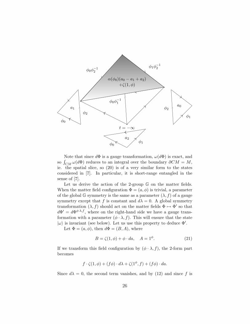
Concretely, a configuration of the “matter field” Φ will be an as-signment of an element of Π1 to every vertex, an element of Π2 toevery edge, Π3 to every face, and so on, for which a single d-simplexis pictured below with 2-group labeling, with φi ∈ Π1, ai ∈ Π2.

3The case of a general d-group is algebraically more involved.

24

t = −∞

φ1

φ0

φ2

a2

a1

a0

Spatial Slice

Triangulation of part of CM , with the cone point at time past infinity.

The ground state in the basis |Φ〉 is

|ω〉 =∑

Φ

exp[2πi

∫CM

ω(dΦ)]|Φ〉. (20)

The integral over CM indicates a sum over all simplices as above. Theintegrand is formed from a cocycle representative ω of the class of theaction (note different representative give different states in the samephase). This d-cocycle is evaluated on each simplex using the labelsgiven by φ. The notation dΦ indicates the induced map CM → BG.It means that we first extend Φ by the identity on all labels on theinterior of CM . Then dΦ is the gauge field generated by a gaugetransformation parametrized by this extension. Finally, ω is evaluatedon this gauge field in the ordinary way to obtain an element of R/Z.We draw it below for the figure above using the rules derived in section4.

25

t = −∞

φ0φ−11

φ0φ−12

φ1φ−12

φ1φ0

a2

a1

φ2

φ0

a0φ2

φ1

α(φ0)(a0 − a1 + a2)+ζ(1, φ)

Note that since dΦ is a gauge transformation, ω(dΦ) is exact, andso∫CM ω(dΦ) reduces to an integral over the boundary ∂CM = M ,

ie. the spatial slice, so (20) is of a very similar form to the statesconsidered in [7]. In particular, it is short-range entangled in thesense of [7].

Let us derive the action of the 2-group G on the matter fields.When the matter field configuration Φ = (a, φ) is trivial, a parameterof the global G symmetry is the same as a parameter (λ, f) of a gaugesymmetry except that f is constant and dλ = 0. A global symmetrytransformation (λ, f) should act on the matter fields Φ 7→ Φ′ so thatdΦ′ = dΦφ·λ,f , where on the right-hand side we have a gauge trans-formation with a parameter (φ · λ, f). This will ensure that the state|ω〉 is invariant (see below). Let us use this property to deduce Φ′.

Let Φ = (a, φ), then dΦ = (B,A), where

B = ζ(1, φ) + φ · da, A = 1φ. (21)

If we transform this field configuration by (φ · λ, f), the 2-form partbecomes

f · ζ(1, φ) + (fφ) · dλ+ ζ(1φ, f) + (fφ) · da.

Since dλ = 0, the second term vanishes, and by (12) and since f is

26

constant, so does the third. We are left with

f · (ζ(1, φ) + φ · da).

Compare with (21). Meanwhile the 1-form part of dΦ′ is simply 1fφ.One can easily check that the same 2-connection can be obtained

by acting on a trivial 2-connection by a gauge transformation parametrizedby Φ′ = (a+φ ·λ+κ(f, φ), fφ), where κ was defined in (18). In otherwords, the global symmetry transformation rules for matter fields are

φ 7→ fφ,

a 7→ a+ φ · λ+ κ(f, φ).

Further, since ω is invariant under the simultaneous action of π1 onitself and on π2, the global symmetry transformation preserves ω(dΦ)and therefore simply permutes the summands in |ω〉, leaving the stateinvariant. Gauging the symmetry leads to the 2-group TQFT withcocycle ω.

8.4 Examples

Let us collect here a couple examples of interesting 2-groups. First isthe 2-group with Π1 = (Z/p)3, Π2 = Z/p, α trivial, and β(a1, a2, a3) =a1a2a3. A crossed module that realizes this 2-group is

Z/p→ UT (p, 3)→ UT (p, 4)→ Z/p3,

where UT (p, k) is the group of upper triangular k × k matrices overFp with 1s on the diagonal (generalizing the Heisenberg group k = 3).The center map places the three northeast elements of a 3× 3 matrixinto the three northeast elements of a 4× 4 matrix.

We have already computed

ζ(a, f) = f1(a2 + df2)(a3 + df3) + a1f2(a3 + df3) + a1a2f3.

andκ(g, φ) = −g1φ2dφ3.

Under a global symmetry transformation parametrized by (g, λ) wetherefore have

φ1 7→ φ1 + g1

φ2 7→ φ2 + g2

27

φ3 7→ φ3 + g3

α 7→ α+ λ− g1φ2dφ3.

Our next example is a 2-group with Π1 = Z/p, Π2 = Z/p, α trivial,and

β(a) = aδa

p,

where a denotes a lift of a, which is ordinarily just defined mod p, toan integer-valued cochain. Thus β is an integer defined mod p. Wehave used this lifting throughout the paper so far, where we mightwrite β = aδa/p, but it will be important for trivializing β that wekeep it explicit here. The derivation is a little bit technical, so onecan feel free to skip to the global symmetry transformations.

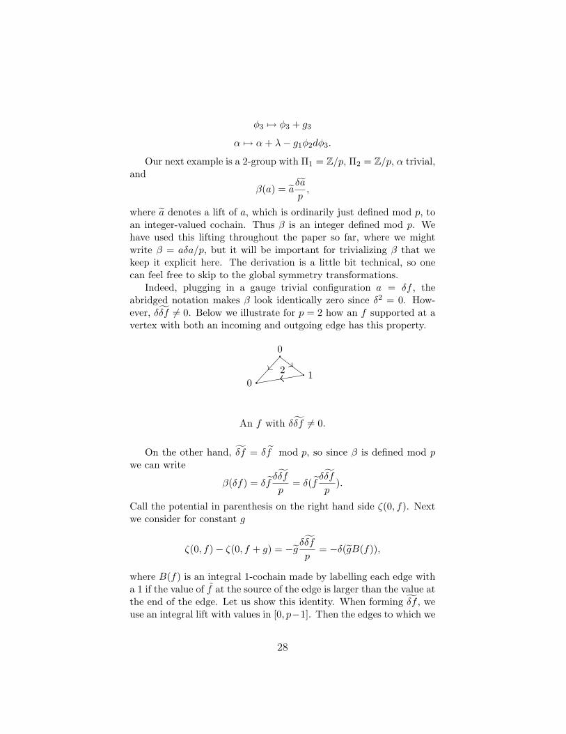
Indeed, plugging in a gauge trivial configuration a = δf , theabridged notation makes β look identically zero since δ2 = 0. How-ever, δδf 6= 0. Below we illustrate for p = 2 how an f supported at avertex with both an incoming and outgoing edge has this property.

10

0

2

An f with δδf 6= 0.

On the other hand, δf = δf mod p, so since β is defined mod pwe can write

β(δf) = δfδδf

p= δ(f

δδf

p).

Call the potential in parenthesis on the right hand side ζ(0, f). Nextwe consider for constant g

ζ(0, f)− ζ(0, f + g) = −g δδfp

= −δ(gB(f)),

where B(f) is an integral 1-cochain made by labelling each edge witha 1 if the value of f at the source of the edge is larger than the value atthe end of the edge. Let us show this identity. When forming δf , weuse an integral lift with values in [0, p−1]. Then the edges to which we

28

must add p to make positive are the ones that are negative. Since δfon an edge 0→ 1 is f1 − f0, this occurs iff f0 > f1. When computingδδf , the values of f all cancel and we are just left with these ps,which we divide by p to get 1s. Putting this together, δδf/p = δB(f).The descendant potential we defined above for this example is thusκ(g, f) = −gB(f).

In the above description of the ground state of an SPT with thissymmetry group, we have matter consisting of Z/p labels φ at verticesand Z/p labels α along edges. Under a global symmetry parametrizedby (g, λ) we have

φ 7→ φ+ g

α 7→ α+ λ− gB(φ).

Gauging this symmetry produces a gauge field with gauge group givenby the 2-group just described.

Appendix: Classifying space of a 2-group

This discussion follows [15]. In this section we implicitly think of Gas a 2-category.

The classifying space of a 2-group G is a topological space BG withG as its homotopy type. We can construct BG inductively as a cellcomplex with 1 0-cell, 1-cells corresponding to 1-morphisms in G, 2-cells corresponding to 2-morphisms, 3-cells corresponding to relationsamong the 2-morphisms, 4-cells added to kill any π3 introduced in theprevious stage, 5-cells added to kill any π4, and so on. Note that therelations among 1-morphisms are imposed by inserting the identity2-morphisms, and any π2 created among these is killed by the 3-cellsimposing the relations among 2-morphisms.

Consider a configuration for the G gauge theory. Using a sections : Π1 → G to make the A variables live in G and including the Bvariables in H, we can interpret this configuration as a composablediagram in G. Mapping each 0-cell of X to the unique 0-cell of BG,1-cells to the 1-cell of the corresponding 1-morphism (an element ofG), and 2-cells to the 2-cell of the corresponding 2-morphism (this isgenerally an element of H but the constraint (3) implies it is actuallyan element of Π2), we obtain a map from the 2-skeleton of X toBG. The 3-cell constraint (4) implies that we can extend this mapto all of X. Changing which section one uses amounts to a gaugetransformation of the original configuration.

29

Conversely, by cellular approximation any map X → BG gives usa configuration for the G gauge theory. Cellular homotopies are gaugetransformations, so we always get gauge-equivalent configurations ifwe pick a different cellular approximation.

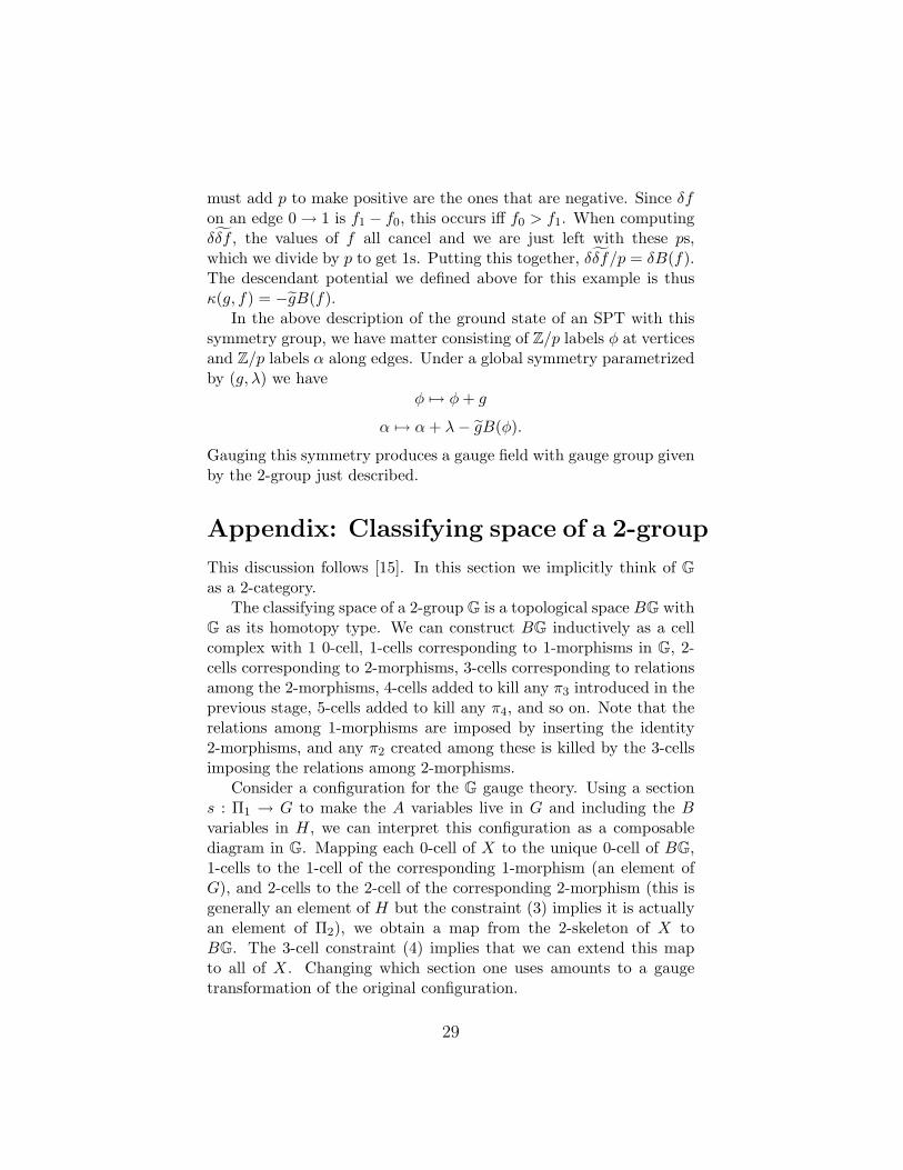
There is a map of 2-groups, which may be thought of as a functor,from G to the group Π1 (considered as a 2-group with only identity2-morphisms) given by identifying isomorphic 1-morphisms in G. Thisgives a map on the 3-skeleton of BG to BΠ1. Since the higher cellsare added to kill homotopy groups for each space, we can inductivelyextend this to a map BG → BΠ1. The fiber of this map over theunique 0-cell of BΠ1 is the classifying space B2Π2 of the group of2-morphisms from the identity 1-morphism to itself. This space hassecond homotopy group Π2 and all others vanishing.

This map is well known to be a fibration

BG

BΠ1

B2Π2

,

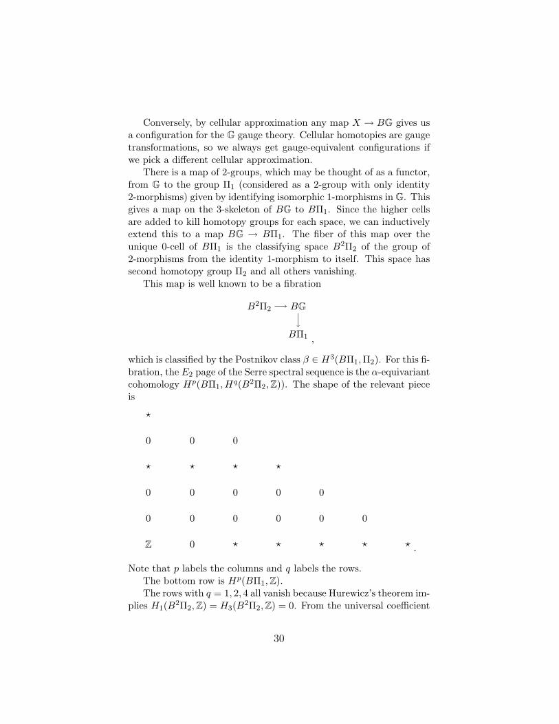
which is classified by the Postnikov class β ∈ H3(BΠ1,Π2). For this fi-bration, the E2 page of the Serre spectral sequence is the α-equivariantcohomology Hp(BΠ1, H

q(B2Π2,Z)). The shape of the relevant pieceis

Z

0

0

?

0

?

0

0

0

?

0

?

0

0

?

0

?

0

0

?

?

0

0

?

0

? .

Note that p labels the columns and q labels the rows.The bottom row is Hp(BΠ1,Z).The rows with q = 1, 2, 4 all vanish because Hurewicz’s theorem im-

plies H1(B2Π2,Z) = H3(B2Π2,Z) = 0. From the universal coefficient

30

theorem it then follows H1(B2Π2,Z) = 0, and since all cohomologyclasses on B2Π2 in positive degree are |Π2|-torsion, the 2nd and 4thcohomology groups also vanish.

The universal coefficient theorem also tells us that H3(B2Π2) =Hom(Π2,R/Z) = Π2, so the q = 3 row is Hp(BΠ1, Π2), where Π1

acts on Π2 via α. For example, H0(BΠ1, Π2) is the subgroup of Π1-invariant characters in Π2.

It is also known that H5(B2Π2,Z) = H4(B2Π2,R/Z) is the groupof quadratic functions q : Π2 → R/Z [22]. The isomorphism is dis-cussed in detail in [3]. The group in the (0, 5) spot in the top left isthen the subgroup of Π1-invariant quadratic forms.

The first possibly non-zero differential is on the E3 page:

H0(BΠ1, H5(B2Π2,Z))→ H3(BΠ1, Π2).

We find it difficult to prove, but we believe that this map sends anelement of the left-hand side, which is a Π1-invariant quadratic formq : Π2 → R/Z to 〈β,−〉q, where the bracket denotes the bilinearpairing 〈x, y〉q = q(x+ y)− q(x)− q(y).

The next possibly non-zero differentials are on the E4 page:

Hj(BΠ1, Π2)→ Hj+4(BΠ1,Z) ' Hj+3(BΠ1,R/Z).

This map is contraction with β.The last relevant possibly non-zero differential is on the E6 page:

H0(BΠ1, H5(B2Π2,Z))→ H6(BΠ1,Z).

We believe this differential is actually zero.This is enough to give the description of the topological actions we

give in section 6.

References

[1] R. Dijkgraaf and E. Witten, “Topological Gauge Theories andGroup Cohomology,” Commun. Math. Phys. 129, 393 (1990).

[2] S. Gukov and A. Kapustin, “Topological Quantum Field The-ory, Nonlocal Operators, and Gapped Phases of Gauge Theories,”arXiv:1307.4793 [hep-th].

[3] A. Kapustin and R. Thorngren, “Topological Field The-ory on a Lattice, Discrete Theta-Angles and Confinement,”arXiv:1308.2926 [hep-th].

31

[4] R. Thorngren, “Electric-Magnetic Duality of Topological GaugeTheories from Compactification,” arXiv:1309.1489 [hep-th].

[5] F. Quinn, “Lectures on axiomatic topological quantum field the-ory,” in: Geometry and Quantum Field Theory, Park City, UT,1991, IAS/Park City Math. Ser. 1, 323-453, AMS, 1995.

[6] D. S. Freed, M. J. Hopkins, J. Lurie and C. Teleman, “Topo-logical Quantum Field Theories from Compact Lie Groups,”arXiv:0905.0731 [math.AT].

[7] X. Chen, Z. -C. Gu, Z. -X. Liu and X. -G. Wen, “Symmetry pro-tected topological orders and the cohomology class of their sym-metry group,” Phys. Rev. B 87, 155114 (2013) [arXiv:1106.4772[cond-mat.str-el]].

[8] M. Levin and Z. -C. Gu, “Braiding statistics approach tosymmetry-protected topological phases,” Phys. Rev. B 86,115109 (2012) [arXiv:1202.3120 [cond-mat.str-el]].

[9] L. -Y. Hung and X. -G. Wen, “Quantized topological terms inweakly coupled gauge theories and their connection to symmetryprotected topological phases,” arXiv:1211.2767 [cond-mat.str-el].

[10] K. Walker and Z. Wang, “(3+1)-TQFTs and Topological Insula-tors,” arXiv:1104.2632 [cond-mat.str-el].

[11] C. W. von Keyserlingk, F. J. Burnell and S. H. Simon, “Three-dimensional topological lattice models with surface anyons,”Phys. Rev. B 87, 045107 (2013) [arXiv:1208.5128 [cond-mat.str-el]].

[12] J. C. Baez, A. D. Lauda, “Higher-Dimensional Algebra V: 2-groups,” arXiv:math/0307200 [math.QA].

[13] A. Hatcher, “Algebraic Topology,” Cambridge University Press,2001.

[14] K. Brown, “Cohomology of groups”, Springer, 1982.

[15] J. Baez and D. Stevenson, “The Classifying Space of a Topolog-ical 2-Group”, [http://arxiv.org/abs/0801.3843 [math.AT]]

[16] J. Baez and U. Schreiber, “Higher gauge theory: 2-connectionson 2-bundles,” hep-th/0412325.

[17] U. Schreiber and K. Waldorf, “Connections on non-abelian gerbesand their holonomy,” arXiv:0808.1923 [hep-th].

32

[18] J. Cheeger and J. Simons, “Differential characters and geometricinvariants,” in: Geometry and Topology (College Park, 1983/84),Springer, 1985.

[19] J. Polchinski, “String theory. Vol. 2: Superstring theory and be-yond,” Cambridge, UK: Univ. Pr. (1998) 531 p

[20] E. Witten, “Quantum Field Theory and the Jones Polynomial,”Commun. Math. Phys. 121, 351 (1989).

[21] O. Aharony, N. Seiberg and Y. Tachikawa, “Reading between thelines of four-dimensional gauge theories,” arXiv:1305.0318 [hep-th].

[22] S. Eilenberg, S. MacLane, “On the groups H(Π, n). II. Methodsof computation,” Ann. Math. (2) 60 (1954) 49.

33