higher order beam theories and isogeometric methods …

International Journal of Bridge Engineering (IJBE), Vol. 5, No. 3, (2017), pp. 133-182

HIGHER ORDER BEAM THEORIES AND

ISOGEOMETRIC METHODS IN THE ANALYSIS OF

CURVED BRIDGES - ASSESSMENT OF

DIAPHRAGMS’ GUIDELINES

Ioannis N. Tsiptsis1 and Evangelos J. Sapountzakis

2

1,2 Institute of Structural Analysis and Antiseismic Research, School of Civil Engineering

National Technical University of Athens, Greece

e-mail: [email protected], [email protected]

ABSTRACT: Towards improving conventional beam elements in order to

include nonuniform warping effects in the dynamic analysis of bridge decks, in

this paper, independent warping parameters have been taken into account and

advanced stiffness matrices have been proposed. In addition to this, curved

beam’s behavior becomes more complex, even for dead loading, due to the

coupling between axial force, bending moments and torque that curvature

produces. Thus, the importance of simulating geometry exactly arises in order

to approximate accurately the response of the curved beam. For this purpose,

the Isogeometric tools (b-splines and NURBS), either integrated in the Finite

Element Method (FEM) or in a Boundary Element based Method (BEM) called

Analog Equation Method (AEM), are employed in this contribution for the

static and dynamic analysis of horizontally curved bridge decks of open (I

girders) or closed (box-shaped) cross section. Free vibration characteristics and

responses of the stress resultants and displacements to static, moving and

earthquake loading have been studied. Design guidelines for intermediate

diaphragms have been applied for different thin-walled box-shaped bridge

decks and assessed as an indirect way to prevent distortional effects.

KEYWORDS: Higher order beam theories (HOBT); curved beam;

Nonuniform torsion; Isogeometric Analysis (IGA); spacing of diaphragms;

1. INTRODUCTION Thin-walled straight or curved structures having open or closed cross-section

are widely used in bridge engineering due to their large bending and torsional

rigidities as well as their low self-weight. As far as their flexural behavior is

concerned, the involved members of these structures are usually analyzed

employing beam elements based on Euler-Bernoulli or Timoshenko beam

theories. Both of these theories maintain the assumption that cross sections

remain plane after deformation. Thus, the formulation remains simple; however

mailto:[email protected]

mailto:[email protected]

134 HOBT and isogeometric methods in the analysis of curved bridges

it fails to capture “shear lag” phenomenon, which is associated with a

significant modification of normal stress distribution due to nonuniform shear

warping [1,2]. This phenomenon has been reported long ago [3-5] in many

structural members such as beams of box-shaped cross sections, folded

structural members or beams of materials weak in shear. In up-to-date

regulations, the significance of shear lag effect in flexure is recognized;

however in order to simplify the analysis and permit the use of available

conventional finite beam elements, the “effective breadth” concept [6-8] is

recommended. This simplifying approach may fail to capture satisfactorily the

actual structural behavior of the member, since the influence of shear lag

phenomenon is not constant along the beam length, while apart from the

geometrical configuration of the cross section it depends also on the type of

loading [9,10]. Similar considerations with the ones made for flexure could be

also adopted for the torsional problem, which is also very often encountered in

the analysis of curved-in-plan bridges. It is well-known, that when a beam

undergoes general twisting loading under general boundary conditions, is

leaded to nonuniform torsion. This problem has been extensively examined in

the literature (e.g. see [11,12]) and its major characteristic is the presence of

normal stress due to primary torsional warping. In an analogy with Timoshenko

beam theory when shear deformation is of importance, Secondary Torsional

Shear Deformation Effect (STSDE) [13,14] has to be taken into account as well.

The additional secondary torsional warping due to STSDE causes similar

effects with shear lag in flexure, i.e. a modification of the initial normal stress

distribution. It is noted that due to the complicated nature of torsion, simplified

concepts such as “effective breadth” cannot be applied to take into account this

behavior.

The above described effects may become substantial in complex structural

forms comprising box-shaped homogeneous or composite cross sections, curved

members, short spans or arbitrary loading. Hence a realistic estimation of stress

state employing conventional beam elements becomes difficult, since generally

commercial programs consider six degrees of freedom (DOFs) at each node of a

member of a spatial frame, ignoring in this way all the warping effects due to

corresponding warping restraint [15-17]. Therefore, it can be concluded that in

order to accurately estimate and assess the actual stress state of a spatial framed

structure more rigorous analyses need to be performed.

Even though refined models based on shell or solid finite elements provide

the means to perform such analyses, the inclusion of nonuniform warping

effects in beam elements based on so-called “Higher-Order Beam Theories”

[18,19] is of increased interest due to their important advantages over more

elaborate approaches. More specifically

A Beam formulation reduces significantly modeling effort (solid models

require cumbersome post- and pre-processing even in relatively simple

Tsiptsis & Sapountzakis 135

cases).

It permits isolation of structural phenomena and results interpretation

contrary to the reduced oversight of the 3-D FEM models (quantities such as

rotation, warping parameter, stress resultants etc. are also evaluated in

contrast to solid model which yields only translations and stress

components).

It allows straightforward model handling (support modeling and external

loading are easily applied).

It avoids difficulties in discretizing a complex structure, while the resulting

increased number of DOFs of the 3-D models leads to severe or unrealistic

computational time.

It avoids difficulties in discretizing a structure including thin-walled

members (shear-, membrane-locking phenomena).

It facilitates parametric analyses (solid modeling often requires construction

of multiple models).

It does not require shape functions for the kinematical components; hence

the minimum number of elements can be employed, while the accuracy of

function derivatives is not compromised.

The use of shell elements cannot give accurate results since warping of the

walls of a cross section cannot be taken into account (midline model).

Comparing to straight beam formulations, the behaviour exhibited by curved

members is far more complex regarding twist deformations. It is well known,

that in case of a horizontally curved beam under transverse loading not only

vertical displacement but twist deformation with respect to its longitudinal axis

arises as well. Regarding curved beam formulations, a series of straight-line

segments is generally used in practice in order to approximate the curved

geometry, though ignoring warping transmission between these segments.

Vlasov [20] presented a solution for curved beams with open arbitrary cross

sections. Then, Dabrowski [21] gave an analysis for closed box-shaped cross

sections. Having in mind the above, it is easily concluded that the influence of

shear lag phenomenon due to both flexure and torsion, which is not constant

along the beam length, should be also considered for curved geometries. The

early curved-beam models that have been formulated are either restricted to the

analysis of only the beam behaviour in the plane of curvature [22] or do not take

into account secondary shear deformation effect caused by nonuniform warping

[23, 24], while other efforts consider only doubly symmetric cross sections [25].

In general, even in recent or past years, although the planar problem has been

extensively studied, comparatively little work has been done concerning the

general three dimensional, non-planar, or coupled lateral-torsional responses of

curved beams [22, 25-28]. Regarding the distortional analysis related to the

intermediate diaphragms, which is more important for box girders, the number

of researches is quite limited. The study related to the distortional analysis of


box girders was initiated by Dabrowski who first formulated the distortional

phenomenon of box members with a symmetric cross section [29]. Later and

more recently, other research efforts were undertaken regarding the distortional

analysis of the structures to give design guidelines on the intermediate

diaphragms. Park et al. in [30] and [31] developed a straight and a curved box,

respectively, beam finite element having nine degrees of freedom per node in

order to propose tentative design charts for adequate maximum spacing of

intermediate diaphragms. However, in most of these studies, the placement of

diaphragms was not related whether to dynamic property analysis or dynamic

response analysis.

When compared to the effort involved in static analysis, there has not been

much effort put into the dynamic analysis of curved box girder bridges [32].

The geometric complexities and the spatial coupling effect between bending

and torsion make the analysis of curved bridges difficult. Bridge design codes

usually provide guidance for the dynamic analysis of straight bridges (dynamic

amplification factor, natural frequencies, modelling of vehicles, placement of

diaphragms etc.). These design recommendations have been used by some

designers for curved bridges, even though some researches carried out [33-35]

revealed that need to be reviewed. When bridges are curved, different kinds of

loads can cause lateral bending and torsional modes of vibration in addition to

the common longitudinal or flexural modes of vibration and so there are still

many possible as well as crucial problems to be investigated regarding the

dynamic response, for example, forced vibration due to moving loads and

earthquake, vehicle-bridge coupling vibration, and wind-induced vibration [36-

38]. Some research efforts analyzed out-of-plane vibrations of beams either

with uniform or varying cross section and curvature [39,40]. In other studies,

the dynamic responses of thin-walled curved box girder bridges due to truck

loading have been investigated. The curved box girder bridges has been

numerically modelled using finite elements which take into account the

torsional warping, distortion and distortional warping [41,42]. However, most

of the previous models have been formulated for specific type of loading and

cross section either considering or not some higher order phenomena.

In this study, the dynamic generalized warping problem of horizontally

curved beams of arbitrary cross section, loading and boundary conditions is

presented. This beam element formulated is employed in the analysis of curved

bridge decks of open or closed (box-shaped) cross section, taking into account

nonuniform warping and shear deformation effects (shear lag due to both

flexure and torsion). Except for these effects, curvature influences also the

internal forces and deformations of the curved continuous beam, even for dead

loading, due to the fact that the curved beam produces coupling between axial

force, bending moments and torque, leading to the development of both angle of

twist and displacement in the radial direction [45]. The numerical solution of

the problem is obtained by Isogeometric tools, either integrated in the Finite


Element Method (FEM) [43] or in a Boundary Element based Method (BEM)

called Analog Equation Method (AEM) [44]. To the authors’ knowledge

Isogeometric analysis is for the first time employed in the design of curved

bridges with higher order beam theories, especially combined with a BEM-

based method. The developed horizontally curved model takes into account

simultaneously in-plane and out-of-plane flexures, extension and torsion and

permits the investigation of their coupling. The structure (e.g. bridge deck) is

subjected to the combined action of arbitrarily distributed or concentrated axial

and transverse loading, as well as to bending, twisting and warping moments.

Its edges are subjected to the most general boundary conditions, including also

elastic support. Nonuniform warping distributions are taken into account by

employing four independent warping parameters multiplying a shear warping

function in each direction and two torsional warping functions, which are

obtained by solving corresponding boundary value problems, formulated

exploiting the longitudinal local equilibrium equation. In this study, the cross

section is considered not deformable in its plane through the presence of a

sufficient number of diaphragms along the bridge deck, preventing distortion.

Design guidelines related to the intermediate diaphragms have been provided to

prevent from excessive distortional warping in the longitudinal direction and

transverse bending deformation along the cross section perimeter. Thus, fixed

values of the stress ratio of the distortional warping normal stress to the bending

normal stress are used. Moreover, having in mind that a rigid diaphragm is

usually placed in the sections over each pier, both the angle of twist and

warping are prevented at these places (bimoment has nonzero values at the

support sections). The assessment of these regulations is carried out in this

research effort through numerical examples and parametric studies. This could

be a natural starting point for the investigation of distortional effects’ impact on

the analysis of curved bridges. Additional degrees of freedom in order to take

into account distortional warping are part of the subsequent research. By

employing a distributed mass model system accounting for longitudinal,

transverse, rotatory, torsional and warping inertia, ten boundary value problems

with respect to the variable along the beam time-dependent 1-D kinematical

components are formulated. Free vibration characteristics and responses of the

stress resultants and displacements to static, moving and earthquake loading

have been studied.

The essential features and novel aspects of the present formulation compared

with previous ones are summarized as follows.

i. The developed beam formulation is capable of the complete analysis (static-

[45] and dynamic-present formulation) of spatial curved beams of arbitrary

closed or open cross section with one plane of constant curvature (either

small or great) considering flexural-torsional shear lag effects and transverse

loading to the plane of curvature (as is usually the case in practice). The


necessity to include nonuniform warping and STSD effects in the dynamic

analysis of curved bridge decks is demonstrated (for the static analysis refer

to [45]).

ii. The numerical solution of advanced beam theories and its application to the

analysis of horizontally curved bridges is based on b-splines [46-47] and

NURBS (Isogeometric Analysis) offering the advantage of integrated

computer aided design (CAD) in the analysis. Comparing to the previous

works of the authors [46-47], where straight beam formulations examined,

regarding the use of Isogeometric tools, the present NURBS’ formulation

allows the integration of the initially curved geometry (which was not

previously the case) in the static and dynamic analysis of the advanced beam

element employing the same basis functions for the representation of the

curve at both deformed and undeformed state. In addition to this, the order of

the basis functions is not predefined and can be adjusted by the user.

iii. The assessment of the design guidelines which specify the maximum

spacing of intermediate diaphragms through comparisons of the proposed

curved model to the corresponding solid or plate ones and some parametric

studies is a first step towards suggesting further provisions and limitations on

the application of these regulations.

Numerical examples are worked out to illustrate the method, designate its

efficiency, accuracy and computational cost, as well as verify its integrity

comparing with the results of traditional methods used for the analysis of

bridges. NURBS and b-splines of various degrees have been employed. Knot

insertion and degree elevation are proved to be very beneficial in refining the b-

spline curve and increasing the accuracy [43]. In addition to this, different radii

of curvature have been applied to the model in order to investigate their impact

on the arising internal forces.

2. STATEMENT OF THE PROBLEM

2.1 Curved beam model and generalized warping Let us consider a curved prismatic element of length L with an arbitrarily

shaped cross section of homogenous, isotropic and linearly elastic material with

modulus of elasticity E and shear modulus G , occupying the region of the

yz plane with finite number of inclusions (Fig.1). The cross section can also be


(a)

(b)

Figure 1. Prismatic curved beam under axial-flexural-torsional loading (a) of an arbitrary

homogenous cross section occupying the two dimensional region (b).

considered as composite. Let also the boundary of the region be denoted by.

This boundary curve is piecewise smooth, i.e. it may have a finite number of

corners. In Fig.1 CXYZ is the principal bending coordinate system through the

cross section’s centroid C , while Cy , Cz are its coordinates with respect to

Sxyz reference coordinate system through the cross section’s shear center S .

It holds that Cy y Y and Cz z Z . The initial radius of curvature is

considered constant, is denoted by R and is parallel to Z axis. The beam

element is subjected to the combined action of arbitrarily distributed or

concentrated axial loading ( )x xp p X along X direction, transverse loading


( )y yp p x and ( )z zp p x along the y , z directions, respectively, twisting

moments ( )x xm m x along x direction, bending moments ( )Y Ym m x ,

( )Z Zm m x along Y , Z directions, respectively, as well as to warping

moments (bimoments) ( )P Px x

m m x

, ( )P PY Y

m m x

, ( )P PZ Z

m m x

and

( )S Sx x

m m x

(Fig.1) [1]. The possible external loading of warping moments

is defined in [45].

Under the action of the aforementioned arbitrary external loading and of

possible restraints, the beam member is leaded to nonuniform flexure and/or

nonuniform torsion. Starting with the flexural behavior of the beam, the

following remarks can be made. It is well-known that the bending moment at a

beam cross section represents the distribution of normal stresses due to bending

(primary normal stresses Pxx ). Due to the aforementioned bending moment

variation along the beam length (nonuniform bending), shear stresses arise on

horizontal sections of an infinitesimal curved beam element (Fig.2),

equilibrating the variation of normal stresses due to bending. Cauchy principle

dictates that corresponding shear stresses arise on the plane of the cross section

as well. If the assumption that plane sections remain plane after deformation

(Euler-Bernoulli or Timoshenko beam theories) is maintained, the arising shear

stresses obtain a uniform distribution over the section [1]. However, this

distribution violates local equilibrium since the requirement of vanishing

tractions xn on the lateral surface of the beam is not satisfied. Thus, the

aforementioned shear stresses exhibit a nonuniform distribution over the cross

section’s domain so that both local equilibrium and vanishing tractions xn on

the lateral surface of the beam are satisfied. These nonuniform shear stresses

will be referred to as primary (or St.Venant) shear stresses ( Pxy ,

Pxz ) and lead

the cross section to warp. Furthermore, due to the nonuniform character of this

warping along the beam length a secondary normal stress distribution Sxx is

developed. This normal stress distribution is responsible for the well-known

shear lag phenomenon and it is taken into account by employing an independent

warping parameter multiplying the warping function, which depends on the

cross sectional configuration. The nonuniform distribution of secondary normal

stresses Sxx along the length of the beam results in the development of

secondary shear stresses Sxy ,

Sxz , which equilibrate the variation of

Sxx at an

infinitesimal beam element. The above remarks are also valid for the problem of

nonuniform torsion taking into account secondary torsional shear deformation


effect – STSDE [1, 13 and 14].

Figure 2. Primary stress of infinitesimal curved beam element and additional terms due to

curvature effect. “Perturbed” straight beam formulation.

Within the above described context, in order to take into account nonuniform

flexural and torsional warping (including shear lag effect due to both flexure

and torsion), in the study of the aforementioned element at each node of the

element ends, four additional degrees of freedom are added to the well-known

six DOFs of the classical three-dimensional frame element. The additional

DOFs include four independent parameters, namely x , Y , Z , x multiplying a shear warping function in each direction ( Y , Z ) and two

torsional warping functions ( x , x ), respectively. These DOFs describe the

“intensities” of the corresponding cross sectional warpings along the beam

length, while these warpings are defined by the corresponding warping function

(PY , P

Z , Px , S

x ), depending only on the cross sectional configuration. Thus,

the “actual” deformed configurations of the cross section due to primary (in

each direction) shear and primary, secondary torsional warpings are given as

, ,PY Yx t y z , , ,P

Z Zx t y z , , ,Px xx t y z

and , ,S

x xx t y z at

any time instant and position along the beam longitudinal axis, respectively.

Moreover, additional terms are added due to curvature effect (Fig. 2) and the


curved beam can be treated as a “perturbed” straight beam avoiding a more

refined treatment, which would be more beneficial to geometries with large

curvatures. Force F in Fig.2 stands in general for any additional vector (even

displacement or strain) that will be added as a result of the differential

geometry. Finally, the corresponding stress resultants of the aforementioned

additional DOFs are the warping moments PY

M

, PZ

M

, Px

M

, Sx

M

(bimoments) along the beam length, arising from corresponding normal stress

distributions. These bimoments due to the aforementioned warpings constitute

additional “higher order” stress resultants, which are developed in the

nonuniform shear and torsion theories.

Within the context of the above considerations and for rigid cross section with

respect to in-plane deformation, the displacement components of an arbitrary

point of the beam at any time instant are given as

primary

, , , , , , , , ,

, , , , ,

P S

PY Z x S

u x y z t u x y z t u x y z t

u x t x t Z x t Y x t y z

secondary

, , , , , ,P P SY CY Z CZ x Sx t y z x t y z x t y z (1a)

, , , , ,xv x y z t v x t z x t

, , , , ,xw x y z t w x t y x t (1b,c)

where u , v , w are the axial, transverse and radial beam displacement

components with respect to the Sxyz system of axes, while Pu ,

Su , denote

the primary and secondary longitudinal displacements, respectively. Moreover,

,v x t , ,w x t describe the deflection of the centre of twist S , while ,u x t

denotes the “average” axial displacement of the cross section. ,x x t is the

angle of twist due to torsion, while ,Y x t , ,Z x t are the angles of rotation

due to bending about the centroidal Y , Z axes, respectively. ,x x t ,

,x x t are the independent warping parameters introduced to describe the

nonuniform distribution of primary and secondary torsional warping, while

,Y x t , ,Z x t are the independent warping parameters introduced to

describe the nonuniform distribution of primary warping due to shear.

After establishing the displacement field, the strain-displacement relations

will be used for the curved beam element described in the previous section. The

general shell theory for cylindrical shells [48] can also explain the occurrence of


additional terms. More specifically, the additional terms due to curvature

regarding the axial strain xx are w

R (which stands for the increase in length

due to the radial displacement w according to [49]) and x

R

(which is the

decrease in the bending curvature with respect to Z axis). Thus, assuming

1Z

R [28] for the strain in the tangential direction in cylindrical coordinates,

the axial strain-displacement relation is given as

, , , , ,

primary

1 ( ) Pxxx x x Y x Z x x x S

w Z wu u Z Y

R R R R

, , ,

secondary

1P P SY x CY Z x CZ x x S

Z

R

(2)

According to the shear components of strain

, , , , ,xy x y x x x yv u v z u

, , , , ,xz x z x x x zw u w y u (3a,b)

setting as

,P Zx x x

R

,

PZ x Y

uw

R ,

PY x Zv (4a,b,c)

,S P Zx x x x x x

R

,

T S Zx x x x x x x

R

(4d,e)

,SZ Y x Y

uw

R ,

SY Z x Zv (4f,g)

and neglecting Z

R effect for shear strains (viewed as higher order term by

itself), the shear strain-displacement relations are given as


, , , , ,

primary

P P P P P Pxy Z y CY y Y y CZ y x S y

m m mZ Y z

, , , , ,

tertiarysecondary

S P S P S P S T SZ CY y Y CZ y x S y S y x S y

m m m m m

(5a)

, , , , ,

primary

P P P P P Pxz Z z CY z Y z CZ z x S z

m m mZ Y y

, , , , ,

tertiarysecondary

S P S P S P S T SZ CY z Y CZ z x S z S z x S z

m m m m m

(5b)

It is worth here noting that in eqn. (4a), the term Z

R

has been added to the

primary shear strain due to torsion Px according to the concept presented in

Fig. 2. Additionally, the primary transverse shear strain PZ due to flexure in XZ

plane (which is the plane of curvature) is given in eqn. (4b), when employing

the equations of general shell theory [48] and considering that the Kirchhoff

hypothesis is not valid ( ,x Yw ). On the contrary, the primary transverse

shear strain PY due to flexure in XY plane is not affected by the curvature and

is given in eqn. (4c). The above mentioned expressions of shear strains are also

analytically derived according to the refined theory of thick cylindrical shells

presented in [50]. Finally, the secondary and tertiary shear strains due to

primary and secondary torsional warping of the cross section are given in eqns.

(4d,e), respectively, while similarly, the secondary transverse shear strains due

to warping in XZ and XY planes of the cross section are given in eqns. (4f,g) ,

respectively.

Employing the Hooke’s stress-strain law, the resulting components of the

Cauchy stress tensor can be obtained after substituting the components of the

strain tensor given in eqns. (2, 5) as xx xxE , xy xyG and xz xzG .

However, as stated above, attention should be paid to the fact that the terms

,S PZ CY iG , ,

S PY CZ iG , ,

T Sx S iG ( ,i y z ) are not capable of representing an

acceptable shear stress distribution, leading to violation of the longitudinal local

equilibrium equation and the corresponding zero-traction condition on the

lateral surface of the beam. Thus, a correction of stress components is

performed without increasing the number of global kinematical unknowns


according to [1] and [45]. In order to establish the differential equations of

equilibrium based on the corrected shear stresses, the principle of virtual work

is employed. The geometric constants of the curved beam’s cross section are

given and explained in [45]. The stress resultants expressed in terms of the

kinematical components can be derived according to [1] and [45]. Using the

expressions of the strain components (eqns. (2, 5)), the definitions of the

stresses and applying the principle of virtual work or any other variational

principle following standard arguments in the calculus of variations, the

governing differential equations for the curved beam in terms of the kinematical

components can be derived. Thus, the local stiffness matrix tk of the spatial

curved beam can be evaluated after solving the system of the linear equations.

Finally, substituting equations of stress resultants to the differential equations of

the curved beam, the equations of equilibrium of the beam are derived as

,z

x x

QN p

R (6a)

,y x yQ p ,z x z

NQ p

R (6b,c)

,t

Z x y Z

MM Q m

R ,Y x z YM Q m (6d,e)

,P PCZ CZ

Syx

M Q m

,P P

CY CY

Szx

M Q m

(6f,g)

,Z

t x t

MM m

R (6h)

,P PS S

S Tt tx

M M M m

,S S

S S

Ttx

M M m

(6i,j)

where the externally applied loads are related to the components of the traction

vector applied on the lateral surface of the beam xt , yt , zt as

d , , ,i ip x t s i x y z

(7a)

dt z ym x t y t z s

(7b)

dY xm x t Z s

dZ xm x t Y s

(7c,d)

d , , , ,P P P Si x S CY CZ Sm x t i s i

(7e)

The governing differential equations are subjected to the corresponding

boundary conditions, which are given as

1 2 3ba u N 1 2 3byv V 1 2 3bzw V (8a,b,c)

1 2 3Z bZM 1 2 3Y bYM (8d,e)


1 2 3PCZ

Z bM

1 2 3P

CYY b

M

(8f,g)

1 2 3x btM 1 2 3PS

x bM

1 2 3SS

x bM

(8h,i,j)

at the beam ends ( 0,x L ), where the reaction forces bN , byV , bzV , bZM ,

bYM , PCYb

M

, PCZb

M

, btM , PSb

M

, SSb

M

are the stress resultants at the

beam ends.

Finally, , , , , , , , ,k k k k k k k k k k ( 1,2,3k ) are functions

specified at the boundaries of the beam ( 0,x L ). The boundary conditions

(eqns. (8)) are the most general boundary conditions for the problem at hand,

including also the elastic support. It is apparent that all types of the

conventional boundary conditions (clamped, simply supported, free or guided

edge) can be derived from these equations by specifying appropriately these

functions (e.g. for a clamped edge it is

1 1 1 1 1 1 1 1 1 1 1 ,

2 3 2 3 2 3

2 3 2 3 2 3 2 3 2 3 2 3 0 ).

2.2 Curved beams and equations of motion In order to derive the differential equations of motion with respect to the

kinematical components, the terms of inertia contributions

mass , , , dtt tt ttVW u u v v w w V have to be added in the previous

and constitutive equations should be employed. is the density of the material

and , ,u v w are the generalized displacements as previously described. Thus,

the generalized vibrational beam behaviour is described by the differential

equations given in eqns. (9) and the spatial mass matrix tm can finally be

derived. Unlike the stiffness matrix and mass matrix of structure, it is not

necessary to construct the global damping matrix from the element damping

matrix by assembling technique and thus no damping matrix of element is

needed to be derived. Much commercial software employs Rayleigh damping

which is a linear combination of mass matrix and stiffness matrix. For the

proposed curved beam formulation damping is neglected.

, , ,, ,2

,

2x xx xYY

xx Y xx

P S SZ Z x Y Z Y

w u wEIEA u

R R R R

G u GA A w A

R R R


,S S S T S TCY S CY S CY S

Zx x x x

G GD D D

R R R

,

inertial contribution

tt xAu p (9a)

, , ,

,, , ,S S S T S T

CZ S CZ S CZ S

P S SY Y xx Z x Y Z x

Z xx x x xx x x

G A A v GA

G D D GDR

, ,


tt C x tt yA v z p (9b)

,, , , S S S T

CY S CY S

xP S SZ Z xx Y x Z Y x

uG A A w GA G D D

R

,, , , ,S T

CY S

Z xx x x xx x x x

EA wGD u

R R R

,

, , ,2 2


2xYY

Y x tt C x tt z

uEI wA w y p

RR R

(9c)

,, ,

,S S S TCZ S CZ S

x x P S SZZ Z xx Y Y x Z Y Z

Zx x x

EI G A A v GAR

G D DR

,S T S S S TCZ S CZ S CZ S

x Z x Z

GGD D D v

R

,

,

S S S TCY S CY S

Y x Y

S T Zt t x x x

G uD D w

R R

GI I

R R

, ,


T P Zt x t x x ZZ Z tt Z

G GI I I m

R R R

(9d)


,, ,

2 xYYYY Y xx xx

wEIEI u

R R

,

P S SZ Z x Y Z Y

uG A A w GA

R


Zx x x xG D D GD

R

,


YY Y tt YI m (9e)

, , , ,P P P P P SCZ S CZ CZ CZ S

Sx xx Z xx x xx Y Z x ZE I I I GA v

,S S S T S TCZ S CZ S CZ S

Zx x x xG D D GD

R

, , ,


P P P S P P PCZ S CZ S CZ CZ CZ

x tt x tt Z ttI I I m

(9f)

, , , ,P P P P P SCY S CY CY CY S

Sx xx Y xx x xx Z Y x Y

uE I I I GA w

R


Zx x x xG D D GD

R

, , ,


P P P S P P PCY S CY S CY CY CY

x tt x tt Y ttI I I m

(9g)

,,, ,

, ,Z x Z xP S T T

t x xx t t x xx t x xx xGI G I I GIR R

, , ,S S S T S S S TCZ S CZ S CY S CY S

Z x xx Z xG D D v G D D

,, , , ,

x xY x xx Y x ZZ Z x

u Ew I

R R R

, , ,


C tt C tt p x tt tA z v y w I m

(9h)

, , , ,P P P P P PS S CY S CZ S

S T Zx xx Y xx Z xx t t x x xE I I I G I I

R

,S S S T S S S TCZ S CZ S CY S CY S

Tt x Z x ZGI G D D v G D D


, , , ,


P P P P P P PS S CY S CZ S S

Y x Y x tt Y tt Z tt

uw I I I m

R

(9i)

, , , ,P S P S S SCY S CZ S S S

T ZY xx Z xx x xx t x x x xE I I I GI

R

, ,S T S TCZ S CY S

Z x Z Y x Y

uGD v GD w

R

, , ,


S S SP S P SS S SCY S CZ S

x tt Y tt Z ttI I I m

(9j)

The above governing differential equations except for the boundary conditions

(eqns. 8) are also subjected to the initial conditions ( 0,x L )

0,0 u x u x , 0,,0t tu x u x (10a,b)

0,0 v x v x , 0,,0t tv x v x (10c,d)

0,0Z Zx x , 0,,0Z t Z tx x (10e,f)

0,0 w x w x , 0,,0t tw x w x (10g,h)

0,0Y Yx x , 0,,0Y t Y tx x (10i,j)

0,0 x xx x

, 0,,0x t x tx x (10k,l)

0,0x xx x , 0,,0x t x tx x (10m,n)

0,0x xx x , 0,,0x t x tx x (10o,p)

0,0Y Yx x , 0,,0Y t Y tx x (10q,r)

0,0Z Zx x , 0,,0Z t Z tx x (10s,t)

After establishing the stiffness and mass matrices of the spatial curved beam

element the equation of motion in matrix form can be given as follows

{ } { }t i t i tm U k U p (11)

where tm , tk are the generalized mass and stiffness matrices, respectively.

tp is the load vector which is equal to 0 for the free vibration case. { }iU

is the vector containing the second derivatives of the different kinematical

components with respect to time while{ }iU is the generalized unknown vector

containing the values of the kinematical components and their first derivatives,

which will be evaluated numerically.


The natural frequencies and modes in which the beam vibrates for the different

motions can be obtained by separation of variables ,iu x t which is assumed

to have the form

, i ti iu x t u x e (12)

where iu x is a function of only the spatial variable x , while 1i , and

is the natural frequency. Inserting (12) into (11) and dividing by the

common exponential term results in the following typical generalized

eigenvalue problem

2 0t t ik m u (13)

which can be tackled through any solver.

3. NUMERICAL SOLUTIONS FOR CURVED BEAMS

3.1 A BEM-based method combined to isogeometric analysis

The evaluation of the kinematical components ,u x t , ,v x t , ,w x t ,

,x x t , ,Y x t , ,Z x t , ,x x t , ,Y x t , ,Z x t and ,x x t

is

accomplished using the AEM [44]. These have continuous derivatives up to the

second order with respect to x at the interval 0, L and up to the first order at

0,x L and up to the second order with respect to t , satisfying the initial-

boundary value problem described by the coupled governing differential

equations of equilibrium (eqns. (9)) along the beam, the initial conditions (eqns.

(10)) and the boundary conditions (eqns. (8)) at the beam ends 0,x L .

According to this method, for these functions, the following relation is valid

2

2

( , )( , )i

i

d u x tq x t

dx (14)

where ( , )iu x t are the different kinematical components and ( , )iq x t are the

corresponding fictitious loads ( 1,...,10i ). Eqns. (14) are quasi-static, i.e. the

time variable appears as a parameter and they indicate that the solution of eqns.

(9), (8), (10) can be established by solving eqns. (14) under the same boundary

conditions (eqns. (8)), provided that the fictitious load distributions ( , )iq x t (

1,...,10i ) are first established. Isogeometric tools have been employed to

approximate both geometry and the fictitious load curve.

The fundamental solution of eqn. (14) is a partial solution of the following

differential equation

2

i2

d u ( x, )( x )

dx

(15)


where iu ( x, )and its derivatives are given as

1

( , ) 1( , ) sgn

2

idu xx r

dx

(16a)

2

1( , ) ( , )

2ix u x r (16b)

with , ,r x x points of the beam.

Employing this fundamental solution, the integral representation of the

kinematical components is obtained as

2 2 100

( , )( , ) ( , ) ( , ) ( , ) ( , ) ( , )

LL

ii i i

du x tu t x q x t dx x x u x t

dx

(17)

Eqn. (17) implies that if ( , )iq x t and all boundary values ( ( , )iu x t , ( , )idu x t

dx) at

the beam ends 0, L are known, ( , )iu x t can be calculated at any internal point

of the beam. Differentiating eqn. (17), the expressions for the derivatives of

( , )iu x t are derived as

1 100

( , ) ( , )( , ) ( , ) ( , )

LL

i ii

du t du x tx q x t dx x

dxd

(18)

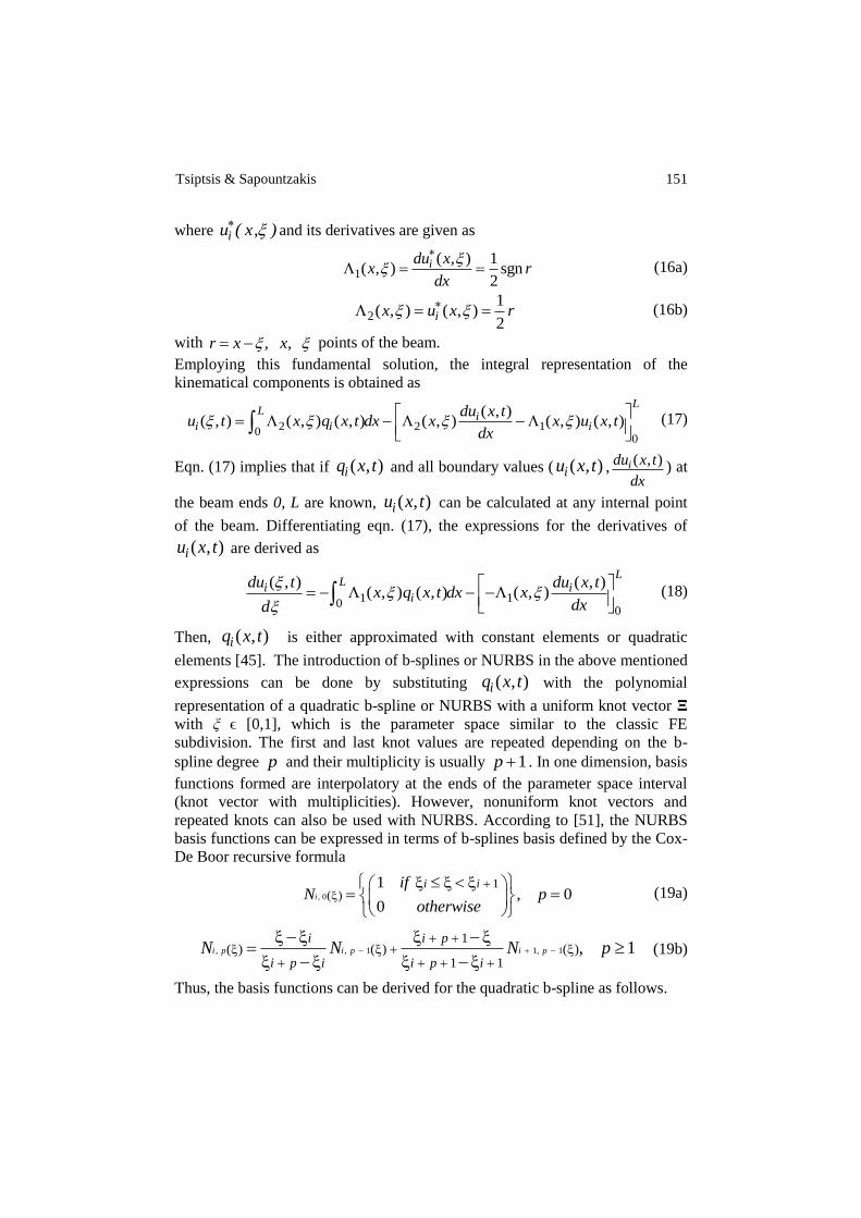
Then, ( , )iq x t is either approximated with constant elements or quadratic

elements [45]. The introduction of b-splines or NURBS in the above mentioned

expressions can be done by substituting ( , )iq x t with the polynomial

representation of a quadratic b-spline or NURBS with a uniform knot vector Ξ

with ξ ϵ [0,1], which is the parameter space similar to the classic FE

subdivision. The first and last knot values are repeated depending on the b-

spline degree p and their multiplicity is usually 1p . In one dimension, basis

functions formed are interpolatory at the ends of the parameter space interval

(knot vector with multiplicities). However, nonuniform knot vectors and

repeated knots can also be used with NURBS. According to [51], the NURBS

basis functions can be expressed in terms of b-splines basis defined by the Cox-

De Boor recursive formula

, 0

1( )

1, 0

0i

i iifN p

otherwise

(19a)

, , 1 1, 1

1( ) ( ) ( )

1 1, 1i p i p i p

i i p

i p i i p iN N N p

(19b)

Thus, the basis functions can be derived for the quadratic b-spline as follows.


2

( )0,2 0,1 1,1

0 1 (1 ) 0

0 0 1 0 0

ifN N N

otherwise

(20a)

( )1,2 1,1 2,1

0 1 2 (1 ) 0

1 0 1 0 0

ifN N N

otherwise

(20b)

2

( )2,2 2,1 3,1

0 1 0

1 0 1 1 0

ifN N N

otherwise

(20c)

The quadratic b-spline curve is defined by

2

,2

0

( ) ( )i i ii

i

C N P

(21)

where iiP are the control points 0iP , 1iP and 2iP of the initial control polygon

shown in Fig. 3. Substituting basis functions to eqn. (21), the expression of the

fictitious load ( , )iq x t at any time instant is derived as

2 2 20 0 0 1 1 2( , ) 2 2 2i i i i i i iq x t P xP x P xP x P x P (22)

Three equidistant collocation points have been used, which are presented in the

same figure with the control points (Fig. 3). These points are on the longitudinal

axis of the curved beam.

Figure 3. Beam element, representation of fictitious load q(x,t), initial control and collocation

points for a kinematical component.

Considering the cubic b-spline, the expression for the fictitious load ( , )iq x t is

derived as


3 2 2 3

0 1 2 33 3 3 3

( ) 3 ( ) 3 ( )( , )i i i i i

l x x l x x l x xq x t P P P P

l l l l

(23)

where iiP are the control points 0iP , 1iP , 2iP and 3iP .

If four equidistant collocation points for discretization are used, the control

polygon of the fictitious load curve and the collocation points are presented in

Fig. 4.

Figure 4. Representation of fictitious load q(x,t) for the cubic b-spline, control and collocation

points for a kinematical component (the control polygon is presented in dashed line).

Similarly, the expression for the fictitious load ( , )iq x t for the quartic B-spline

is derived as 4 3 2 2

0 1 24 4 4

3 4

3 44 4

( ) 4 ( ) 6 ( )( , )

4 ( )

i i i i

i i

L x x L x x L xq x t P P P

L L L

x L x xP P

L L

(24)

where iiP are the control points 0iP , 1iP , 2iP , 3iP and 4iP .

Eqns. (17) and (18) written for the boundary points constitute a system of four

simultaneous integral equations, while the boundary conditions (8) are

formulated in matrix form giving four more equations. Combining the

aforementioned equations, the following system is derived

11 12 1 1

21 22 2 2

{ } {0}{ }

{ } { }{0}

ii i

i i

E E u DE u D T

E E u T

(25)

where [ ]E is a square 40x40 matrix, { }iu ,{ }D ,{ }iT are 40x1 vectors, 11[ ]E ,


12[ ]E are 20x20 known coefficient matrices and 1{ }D is 20x1 known

coefficient vector, all given in the following equations.

21 1 22 2 2[ ]{ } [ ]{ } { }i iE u E u T (25a)

1

2 00

2 1

2 00

( , ) ( , ){ }

( , ) ( , )

i

i

i

x q x t dxT

x q x t dx

(25b)

'

1{ } (0) (0)T

i i iu u u (25c)

'

2{ } (1) (1)T

i i iu u u (25d)

2 0 1 0

21

2 1 1 1

(0, ) ( (0, ) 1)

(0, ) (0, )E

(25e)

2 0 1 0

22

2 1 1 1

(1, ) (1, )

(1, ) ( (1, ) 1)E

(25f)

11 1 12 2 1[ ]{ } [ ]{ } { }i iE u E u D (25g)

2

0{ } { }

{ }i i i i

i

T P T F PT

(25h)

Thus, the following system is derived from eqns. (25) and (25h)

1 1

i i i iE u D F P u E D E F P

(26)

With known values at beam ends and applying the integral representations (17)

and (18) at the internal collocation points, the following can be calculated

{ } [ ] [ ]i i iU A P C u (27a)

' '{ } [ ] [ ']i i iU A P C u (27b)

where '( , )i iU U are the vectors containing the values of the different

kinematical components and their first derivative at internal collocation points.

The coefficients of the square matrices [ ],[ ']A A are given by the numerical

solution of the integrals in eqns. (28a, b). The [ ],[ '],[ ''],[ ''']C C C C matrices

are given in eqns. (28c, d).

2( , ) ( , )j

i iA x q x t dx

(28a)

1' ( , ) ( , )j

i iA x q x t dx

(28b)


2 1 1 1 2 1 1 1

2 2 1 2 2 2 1 2

2 3 1 3 2 3 1 3

(0, ) (0, ) ( , ) ( , )

(0, ) (0, ) ( , ) ( , )

(0, ) (0, ) ( , ) ( , )

l l

C l l

l l

(28c)

1 1 1 1'

1 2 1 2

1 3 1 3

(0, ) 0 ( , ) 0

(0, ) 0 ( , ) 0

(0, ) 0 ( , ) 0

l

C l

l

(28d)

Substituting eqn. (26) into eqns. (27a, b), the following are derived

{ } [ ]i iU B P R (29a)

'{ } [ '] 'i iU B P R (29b)

where

1

B A C E F

(30a)

1

' ' 'B A C E F

(30b)

1

{ }R C E D

(30c)

1

{ '} 'R C E D

(30d)

Then, the stiffness and mass matrices of the beam element, which behavior is

described by eqns. (9) for the dynamic problem, can be calculated employing

eqn. (11). Eqns. (9) can be re-written as follows

[ ] [ ]t t t t tm B q k B q p (31)

where tq in the AEM combined with b-splines or NURBS are the values of

the control points while [ ]B contains the coefficients of B and 'B matrices.

The diagonal matrix 0[ ]A is also determined and contains the values of basis

functions , ( 1... 2... )i jN i n and j p for the n different collocation points

and different p-degree b-spline cases. Then, ,tm tk are formulated and eqn.

(31) is solved.

Instead of b-splines, NURBS curves in terms of b-spline basis functions can

be employed in the AEM technique. Their expressions are given in the

following section.


3.2 FEM and NURBS numerical solutions The problem described in section 2.1 can be set in the equivalent variational

formulation through the principal of virtual work and finally derive eqns (9). In

order to discretize eqns. (9), the displacement field iu x given in section 3.1

is approximated by means of polynomial interpolating functions of p-degree as

extensively is described in [52]. Substituting the displacement approximation

for each discretization element (n in total), the equilibrium equations in terms of

the nodal displacements of the finite element mesh can be expressed. Thus,

tk matrix can be obtained by assembling the contributions from the

individual elements. This can be performed numerically by using the Gauss

quadrature rule. In order to compute Gauss base points and weight factors an

algorithm has been employed according to [53]. The same procedure can be

followed in the AEM technique, with quadrature nodes being the collocation

points, if the analytical solution of the integrals employed needs to be avoided

for computational reasons. The assembling of “stiffness” matrix [ ]B

is

different in this case, too.

As a next step in discretizing eqns. (9), p-degree NURBS interpolating

functions can be employed for the representation of the displacement field

iu x . In this case, curve C given in eqn. (21) has a p-degree NURBS

representation defined by

,

1

( ) ( )n

i i p ii

i

C R P

(32)

where iiP are the control points employed for each kinematical component and

, ( )i pR , which are the NURBS basis functions, can be expressed as follows

,

,

,

1

( )( )

( )

i p ii p n

i p i

i

N wR

N w

(33)

where , ( )i pN are given in eqns. (19) and iw ( ) are weights related to the

ith control point and increase the capabilities of the b-splines interpolation

([43]). Values of the basis functions and their derivatives will be obtained for

each quadrature node. It should be noted that if all weights are equal, then

, ,( ) ( )i p i pR N and curve C is a b-spline curve. In addition to this, the

geometry of the beam is described by a NURBS structure through an initial

control polygon given by the following spatial coordinates ( , , , )i i i ix y z w . This

polygon will be later refined as new knots will be inserted and degree will be


elevated in order to achieve more accurate results. tk matrix can finally be

obtained following the same procedure as previously described for the AEM

technique.

Non-uniform knot vectors Ξ and repeated knots are the key ingredients of

NURBS flexibility. In addition to this, among all the properties of NURBS

interpolation the most interesting is the high degree of continuity ([43]).

4. NUMERICAL EXAMPLES - ASSESSMENT OF DIAPHRAGMS’

GUIDELINES In order to validate the proposed formulation of the curved beam element

described above and examine the advantages attained by the use of the methods

proposed in terms of simplicity, accuracy and computational effort, computer

programs have been written and representative examples have been studied. The

numerical results have been obtained employing NURBS, beam FEs and

constant or quadratic elements for the representation of the AEM fictitious

loads. Then, the results are compared to those obtained by the application of the

Finite Element Method (FEM) employing beam, solid (quadrilateral or

triangular) or plate elements. The computer software FEMAP 2008 [54] has

been used for this purpose. In addition to these, up to 400 boundary elements

depending on the cross section type (cross sectional discretization) have been

employed in order to evaluate the geometric constants with BEM.

As another part of this section, design guidelines for specifying the

maximum spacing of intermediate diaphragms have been applied to the

aforementioned solid models and compared to the proposed one which does not

take into account distortional effects. Three different examples of box-shaped

cross sections subjected to different geometric limits have been examined.

According to thin-walled theory, the upper bounds of these limit sets are

/ 0.1t d and / 0.1d L , where t , d and L are the thickness, width and

length of the curved box-shaped cross section, respectively.

4.1 Extremely thin-walled monosymmetric box-shaped cross section

( / 0.02t d , / 0.1d L ) In this example, in order to investigate the importance of warping in the

analysis of beams as proposed in this study as well as the placement of

intermediate diaphragms, the static problem of a monosymmetric box shaped

straight cantilever bridge beam during its erection phase is examined. Its cross

section is shown in Fig. 5 (7 24 10E kN m ,

7 22 10G kN m - these

properties have been selected for comparison reasons and give 0 ,

2 47.85kN sec / m , 10L m , R ) under a concentrated load


1000yP kN in the vertical direction eccentrically applied at its free end. In

Table A.1 of the Appendix the geometric constants of the cross section are

presented.

In Fig. 6 a model of the beam implemented in FEMAP [54] employing

FEM quadrilateral solid elements is shown. In the same figure the total

deflection is also recorded. It is worth here noting that in order to obtain the

distributions of the kinematical components and stress resultants from the solid

model, rigid diaphragms were placed in regular distances (20 in total),

permitting the measurement of rotation angles and translations of the reference

nodes. The existence of diaphragms also ensured the absence of local

distortional phenomena of the cross sectional profiles. Results coincide with the

beam formulation of the present study.

Figure 5. Box-shaped cross section of the beam of example 4.1.

Figure 6. Model in FEMAP employing 780 quadrilateral solid finite elements. Deflection w(x) is

displayed along the length of the beam.

Y

Z


The Guide Specifications for Horizontally Curved Highway Bridges by the

AASHTO [55] specify the maximum spacing of the intermediate diaphragms

DL as

1/2

25200 7500

D

RL L ft

L

where L and R denote the span length

and radius of curvature in feet, respectively. This provision meets the

requirement that the distortional warping normal stress is limited within 10% of

the bending normal stress and the transverse bending normal stress is limited to

137.3MPa or lower. In addition to this, the Hanshin Expressway Public

Corporation of Japan provided the Guidelines for the Design of Horizontally

Curved Girder Bridges [56], specifying the maximum spacing of the

intermediate diaphragms in curved box girder with respect to that in straight

box girders multiplied by a reduction factor, which is equal to unity for a span

length less than 60 m. It should be noted here that the boundary conditions and

the cross section shape are not taken into account for both specifications

directly.

According to these guidelines, Fig. 7(a) shows the deformed shape and total

translation of the beam displayed in Fig. 6 employing 2 diaphragms (one at

midspan and one at the free edge) while Fig. 7(b) is the same but without the

employment of any diaphragms. Results of models displayed in Figs. 6 and

7(a), which are similar to each other, almost coincide with the results obtained

by the proposed beam formulation. However, it is obvious from Fig. 7(b) that

the absence of diaphragms leads to a larger total translation by 18% due to the

development of distortional warping. Thus, the proposed beam formulation can

predict a highly accurate behavior of the 3d model in terms of simplicity and

safety and comply with the guidelines without considering any distortional

effects.

(a)


(b)

Figure 7. Deformed shapes and total vertical translation of the beam of example 4.1 (a) for 2

diaphragms and (b) without diaphragms.

Then, the same beam is considered curved having the same length and a radius

of curvature 6.366R m forming an arc of 90° angle in top view. In Fig. 8

two models of the beam implemented in FEMAP [54] employing FEM

quadrilateral solid elements are shown. The difference between the two models

is in the use of diaphragms in the cross section plane. In the first one 13

diaphragms have been employed while in the second model only one. The

bridge beams are subjected to a vertical concentrated load 1000yP kN

applied at the centroid of their free end cross sections. In the same figure the

total deflections are also recorded. It is worth here noting that the placement of

the rigid diaphragms along the length of the curved beam becomes quite

cumbersome due to the complexity of the solid model. In addition to this, much

more quadrilateral solid elements have been employed comparing to the straight

beam formulation (Fig. 6) for accuracy reasons. Comparing the deformed

shapes of the beams, it is obvious that the existence of diaphragms ensures

indeed the absence of local distortional phenomena of the cross sectional

profiles along the arc length while the total maximum translation is reduced by

46%. Due to the very thin-walled structure of the cross section, a plate model in

FEMAP [54] has also been employed for comparison reasons with the solid

model and in order to detect any possible locking phenomena present.

In Table 1 the values of the kinematical components v x , x x and Z x

for the vertical force yP concentrically applied at the free edge of the beam

are presented for i) proposed curved beam elements with NURBS (cubic) , ii) a-

1500 quadrilateral plate elements with 13 diaphragms (FEMplate 13 Diaph.), ii)

b- 1500 quadrilateral plate elements with 1 diaphragm (FEMplate 1 Diaph.), ii)

c- 1500 quadrilateral plate elements with 2 diaphragms (FEMplate 2 Diaph.)


according to guidelines previously mentioned, iii) 10976 quadrilateral solid

elements with 13 diaphragms in FEMAP 2008 (FEMsolid 13 Diaph.), iv) 10976

quadrilateral solid elements with 2 diaphragms in FEMAP 2008 (FEMsolid 2

Diaph.) according to guidelines previously mentioned and v) 10976

quadrilateral solid elements with one diaphragm in FEMAP 2008 (FEMsolid 1

Diaph.). Analysis with cubic NURBS gives results closer to the solid model

with diaphragms as it is expected. The results obtained by the analysis of the

solid model with diaphragms almost agree with those obtained by the plate

model with diaphragms (discrepancies around 1%). However, it is important to

notice that the results obtained by the respective models with only 1 diaphragm

differ from each other (discrepancies vary from 15 to 23%). The solid model

seems to be stiffer than the plate one while the different displacement values are

exclusively related to distortional phenomena (mainly attributed to torsion)

since the corresponding models with diaphragms (no distortion) show the same

level of accuracy.

(a)

(b)

Figure 8. Deformed shapes of models in FEMAP employing 10976 quadrilateral solid finite

elements and (a) 13 diaphragms or (b) one diaphragm.


Table 1. Kinematical components of the beam of Figure 5 for vertical load

( )v m

at x=L

( )x rad

at x=L

( )Z rad

at x=L

4 cubic NURBS 0.4879 -0.0202 -0.0742

FEMplate

13 Diaph. 0.4701 -0.0231 -0.0691

FEMplate

2 Diaph. 0.5516 -

0.02902 -0.0812

FEMplate

1 Diaph. 0.9748 -0.0951 -0.1470

FEMsolid

13 Diaph. 0.4647 -0.0229 -0.0685

FEMsolid

2 Diaph. 0.5346 -0.0279 -0.0790

FEMsolid

1 Diaph. 0.8215 -0.0726 -0.1235

It is worth here noting that if diaphragms are placed in the solid model

according to the guidelines (2 diaph. case), the vertical translation is more than

the proposed formulation by 8.7%. Additionally, the angle of twist is increased

by 25% and the angle of rotation due to bending by 6%. Discrepancies are

slightly larger comparing to the corresponding plate model. The proposed

curved beam element is obviously more strict regarding the placement of

diaphragms in terms of safety against distortional effects comparing to solid and

plate models. This implies the use of more diaphragms comparing to the those

specified by the guidelines. In addition to this, comparing stresses between

different solid models, it is proved that the normal stress due to distortion is

more than the specified 10% of the normal stress due to bending for the 2 diaph.

model.

A paramentric study considering different radii of curvature for the same

beam length and cross section has been conducted and different models have

been examined. In Table 2 the discrepancies between the proposed curved beam

formulation and the model with the diaphragmatic arrangement according to the

Py Lateral

Loading


guidelines have been compiled. It is evident that as the curvature of the beam (

1/ R ) becomes greater, the “error” of the specified diaphragmatic model

becomes larger in an exponential rate and this rate seems to be greater for

torsion. In addition to these, considering the solid model with no diaphragms

and comparing to the other models, it seems that distortional effects are of more

importance for large curvatures and a more refined treatment should be

considered. It should also be noted that that the high ratios of the dimensions to

thickness of the cross section’s walls is also an important factor, especially for

torsion.

Table 2. Discrepancies (%) in kinematical components’ values for different

radii of curvature between the proposed model and those according to

guidelines

(%) v

at

x=L

(%)

x

at x=L

(%)

Z

at x=L

R=∞ 0.00 0.64 0.00

R=28.65m 1.09 1.41 1.06

R=12.73m 3.03 3.40 1.91

R=6.37m 8.73 27.60 6.08

The numerical procedure and the dynamic response of the beam are examined

in the following. Particularly, in Fig. 9 the distribution of the vertical deflection

v x for the concentrated load 1000yP kN in the vertical direction

eccentrically applied this time at its free end. Curved beam elements proposed

can accurately give the maximum deflection of the beam model under

consideration. However, the distribution along the X axis of the arc in plan can

satisfactorily be described only by the NURBS approximation of the proposed

beam model due to the fact that the same NURBS functions, as for the

representation of the kinematical components, have been used to describe the

geometry of the curved beam and no post processing computations need to be

done as in FEM beam elements. The discrepancies arising between the

NURBS’ model and the solid one are probably due to the number of the

diaphragms used and their positions along the length, which make the solid

Py eccentric

Lateral

Loading


model stiffer than it should be. Another reason might be shear locking problem.

Additionally, the dynamic problem of the aforementioned curved beam has

been studied and the values of different eigenfrequencies have been compiled in

Table 3 for the same analysis cases as in the previous Table 1. It is obvious that

the analysis employing the proposed curved beam formulation with NURBS

approximation is closer to the FEM solid model with 13 diaphragms while the

eigenfrequencies of the solid model without diaphragms are quite smaller.

However, the diaphragmatic model seems to be stiffer than the proposed model

especially for higher eigenfrequencies. It is also worth noting that convergence

is obtained with few beam elements when NURBS are employed.

Figure 9. v x distributions derived from the analysis of solid and curved beam models of

example 4.1.


Table 3. Eigenfrequencies of the beam of Figure 5

Mode Number FEMsolid

1 Diaph.

FEMsolid

2 Diaph. FEMsolid

13 Diaph.

4 cubic

NURBS

10cubic

NURBS 1 0.1172 0.1416 0.1548 0.1317 0.1317

2 0.2556 0.2615 0.2704 0.2191 0.2191

7 0.3262 0.3644 1.0436 1.1045 1.1042

8 0.3562 0.3799 1.4233 1.2313 1.2311

9 0.4022 0.4761 1.5021 - 1.3345

In Fig. 10 the bending moment distribution is plotted for different methods

employing either the proposed beam elements or the ones used in commercial

software (Timoshenko beam elements). The proposed method is validated. It is

worth noting here that when employing NURBS there is no need for post

processing of data in order to derive stresses and stress resultants as it is the

case in FEM. This is due to the fact that the same basis functions are used for

the representation of geometry and kinematical components.

Figure 10. ZM x

distributions derived from the analysis of curved beam models of example 4.1

and printed directly along with the curved model.

Thus, the matter is just to derive deformations and their first derivative

employing the same NURBS structure for specific locations along the curve of


the beam. In addition to this, when employing AEM much more discretization

elements need to be used for the same accuracy level.

In Fig. 11 the torsional moment and Bimoment distributions are plotted

employing the analysis of the proposed beam model with NURBS on the curved

model directly without any post-processing. Considering commercial FEM

beam elements secondary Torsional Moments and Bimoments are not

considered. However, the magnitude of Bimoment near the fixed support is

around 10% of the total Torsional Moment and should be indeed considered in

the analysis. In addition to this, secondary Torsional Moment varies from 15

(near support) to 0% of the total Torsional Moment and should also be

considered.

Figure 11. Torsional Moment and Bimoment distributions derived from the analysis of the

proposed curved beam model of example 4.1 and printed directly along with the curved model.

Finally, in Fig. 12 the dynamic response of the curved cantilever beam

previously described is plotted in terms of the tip deflection out of the curvature

plane. The eigenfrequency of the first mode is 49.08 rad/sec (T=0.0204

seconds). A static load 2000yP kN applied at the centroid of the free end

has been dynamically applied in three different ways, namely suddenly applied


for 0.025 seconds, gradually applied for the first 0.005 seconds and gradually

applied for 0.015 seconds. It is obvious that the amplification is less severe for

the last case due to the fact that the load rise is more gradual. This is equal to

1.3 while for the case of the suddenly applied load is equal to 1.95. Regarding

the other case of gradually applied load but with a shorter rise time, the

amplification factor is equal to 1.83. Considering a straight beam of the same

length and loading, the amplification factor for the case of transient response is

equal to 1.98.

Figure 12. Deflection v x at the tip of the curved cantilever beam shown in Fig. 8a for different

cases of dynamic loading.

4.2 Moderately thin-walled monosymmetric box-shaped cross section

( / 0.086t d , / 0.086d L ) A cantilever beam of a monosymmetric box-shaped (Fig. 13) cross section

( 7 23 10E kN m , 7 21.5 10G kN m -high strength concrete, 32,5t / m

40L m , 25.465R m ) under a concentrated load 10000yP kN

concentrically applied, as this is shown in Fig. 14 is examined in order to

further validate the proposed beam formulation. In Table A.2 of the Appendix

the geometric constants of the cross section shown in Fig. 13 are presented.



Figure 14. Deformed shape of model in FEMAP employing 2500 quadrilateral solid finite

elements.

In Table 4 the values of the kinematical components v x , x x and Z x

for the vertical force yP concentrically applied at the free edge of the beam are

presented for i) proposed curved beam elements with NURBS (cubic), ii) 2500

quadrilateral solid elements in FEMAP 2008 with 1 or 2 diaphragms (FEMsolid

1 or 2 Diaph), iii) 2500 quadrilateral solid elements with 16 diaphragms

according to guidelines of [55] in FEMAP [54] (FEMsolid 16 Diaph.), iv) 2500

quadrilateral solid elements with 7 diaphragms according to guidelines of [56]

in FEMAP 2008 (FEMsolid 7 Diaph.) v) 2500 quadrilateral solid elements in

FEMAP 2008 with 4 diaphragms (FEMsolid 4 Diaph )and vi) 40 quadratic


elements in the AEM technique (AEM 40 quad.). It is worth nothing here that

when using 16 diaphragms, the vertical displacement is reduced by 23% while

the angle of twist and rotation due to bending are reduced by 10% and 30%,

respectively, comparing to the arrangement with 1 diaphragm. The differences

in the corresponding values of the models with 2 and 4 diaphragms from those

of the model with 1 diaphragm are larger in a disproportionate way when

comparing the corresponding values of the same models to those of the model

with 7 diaphragms. In addition to this, the proposed formulation gives results

closer to the solid model with two diaphragms. Regarding the values of stresses,

the discrepancies in shear stresses between models with 2, 4 and 7 diaphragms

are not of much importance in comparison with those in normal stress.

Additionally, the 2-diaphragmatic model exhibits stresses closer to the model

with 4 diaphragms than that with 1 diaphragm. These imply that distortional

effects are not of the same importance as considered in the guidelines and the

use of the numbers of diaphragms specified make the solid model stiffer than it

should be in real resulting in uneconomic design practices for a case like this

one.

Table 4. Kinematical components of the beam of Figure 13 for vertical load

( )v m

at x=L

( )x rad

at x=L

( )Z rad

at x=L

4 cubic NURBS 0.3197 -0.007029 -0.0104

FEMsolid

1 Diaph 0.3547 -0.00867 -0.0115

FEMsolid

2 Diaph 0.3256 -0.00782 -0.0103

FEMsolid

7 Diaph. 0.2914 -0.00756 -0.0090

FEMsolid

16 Diaph. 0.2746 -0.00778 -0.0081

FEMsolid

4 Diaph. 0.3021 -0.00753 -0.0094

AEM 40 quad. 0.3197 -0.07020 -0.0104

Py Lateral

Loading


Similarly to previous example, in Fig. 15 the distribution of the vertical

deflection v x

along the x axis of the curved geometry in plan for the

concentrated load in the vertical direction mentioned previously. As it is the

case in the previous example, curved beam elements proposed can accurately

give the maximum deflection of the beam model under consideration. It is

worth noting here that the approximation of the v x

distribution when

employing quadratic elements in the AEM technique exhibits a stiffer behavior

comparing to NURBS approximation.

Moreover, the dynamic case is studied and the eigenfrequencies are evaluated

and compiled in Table 5 for the solid model and the proposed one analysed

employing NURBS. The values of the proposed formulation are closer to the

solid model with 1 or 16 diaphragms for the first five eigenfrequencies and

closer to the solid one with 16 diaphragms for the last three. However,

regarding the design quantities, the first eigenfrequencies are of main interest.

Thus, it is implied that distortion can be prevented with few number of

diaphragms.

Table 5. Eigenfrequencies of the beam of Figure 13

Mode Number FEMsolid

1 Diaph.

FEMsolid

16 Diaph. cubic

NURBS

1 0.0488 0.0541 0.0412

2 0.1408 0.1457 0.1203

3 0.1905 0.2208 0.2501

4 0.3002 0.3885 0.3200

5 0.4643 0.5033 0.4452

6 0.5309 0.6481 0.6465

7 0.6299 0.8718 0.7046

8 0.6797 1.0252 0.9412

9 0.7125 1.1320 1.1889

10 0.7361 1.4439 1.3252

In Fig. 16 the distribution of total, primary and secondary Torsional Moments

are plotted along the length of the curved beam for the concentrated load in the

vertical direction. In addition to this, the Bimoment distribution has also been

plotted. It is worth noting here that Torsion and Warping are of the same order

of magnitude near the support for this specific cross section. Thus, Warping

effect will cause important discrepancies between the commercial FEM beam

elements and the one proposed in this study. Secondary Torsional Moment has a

considerable value near support, too.


Figure 15. v x

distributions derived from the analysis of the solid and curved beam models of

example 4.2.

Figure 16. Torsional Moments and Bimoment distributions derived from the analysis of the

proposed curved beam model of example 4.2 and printed directly along with the curved model.


Considering the curved beam of Fig. 14 with fixed end supports and a load

20000yP kN applied at the centroid of the mid span, the amplification

factor of the transient response for is equal to 1.90 for a system’s period

T=0.127 seconds (first mode) at time t=0.0675 seconds.

4.3 Concrete monosymmetric box-shaped cross section ( / 0.1t d ,

/ 0.065d L ) The curved beam of a concrete monosymmetric box-shaped cross section

(7 23,25 10E kN m , 0,1667 - high strength concrete,

32,5t / m ,

33L m , 100R m ) shown in Fig. 17 is examined either as cantilever or

clamped for static and dynamic response. In Table A.3 of the Appendix A the

geometric constants of the cross section are presented.


According to guidelines previously mentioned for the placement of intermediate

diaphragms, either 5 [55] or 6 [56] diaphragms should be at least employed in

order to fulfill limitations. Considering a cantilever beam, as the less favorable

case in terms of boundary conditions, under a concentrated load 3000yP kN

eccentrically applied at its free end, several diaphragmatic arrangements have

been performed.

The distributions of the main displacements and the maximum stresses

arising have been illustrated in Fig. 18. The proposed formulation with NURBS

coincides with the FEM model of 6600 triangular solid elements and one rigid

diaphragm created with FEMAP [54] (errors around 0% for displacements and

stress resultants). The discrepancies between the proposed formulation and the

solid model without any diaphragms are quite small (less than 5%) and only for

the angle of twist the difference becomes larger (8.6 %). This implies that the

distortion is not of much importance for this cross section and structural

arrangement. Regarding the maximum normal and maximum shear stresses, it

seems that the after the placement of 4 diaphragms not much difference takes

place and even for less than 4 diaphragms the “errors” arising are around 5%.

Thus, guidelines might lead to cost ineffective solutions for this particular

curved bridge deck.


Figure 18. Discrepancies from solid model without diaphragms for a cantilever beam with the

cross section shown in Fig. 17.

In addition to these, the clamped model of the same beam is considered in Fig.

19. Similarly to the previous case of the cantilever beam, the proposed

formulation agrees to the solid model with one diaphragm. The discrepancies

between the models become larger for displacements as the number of

diaphragms increases comparing to the previous case of the cantilever beam.

However, stresses, which are of more importance in this case due to the fact that

the magnitude of displacements is quite low, are almost unaffected by the

placement of diaphragms. Thus, it seems that boundary conditions need to be

considered in the specification of diaphragms.


Figure 19. Discrepancies from solid model without diaphragms for a clamped beam with the

cross section shown in Fig. 17.

After specifying the maximum spacing of diaphragms and employing only one,

the dynamic problem of the clamped curved beam is examined. In Table 6 the

eigenfrequencies are compiled for three different cases, namely proposed

formulation, solid model with one diaphragm (FEMAP) and solid model

without diaphragm (ANSYS-SOLID45) [57]. It is important to note that

damping is considered in the last case. However, the eigenfrequencies of the

proposed curved beam formulation are in general quite close to solid model

without diaphragm and in fact are closer than the solid with one diaphragm,

especially after the fifth mode.


Table 6. Eigenfrequencies of the clamped beam shown in Fig. 17

Mode

Number

FEMsolid

1 Diaph.

Solid45

no

Diaph.

cubic

NURBS

Description of the

predominant modes

1 9.72 (1.73)* 9.67

(1.22)* 9.55

First mode of vertical

displacement

2 19.21 (0.65) 19.47

(0.70) 19.33

First mode of lateral bending

3 21.58 (4.62) 21.66

(4.97) 20.58

First mode of torsion

4 22.75 (1.11) 22.98

(2.10) 22.49

Second mode of vertical

displacement

5 33.59

(13.74)

36.57

(4.48) 38.21

6 37.10 (7.93) 38.67

(3.55) 40.04

7 44.16 (3.50) 43.74

(2.57) 42.61

8 47.68

(11.84)

51.39

(3.78) 53.33

*() difference between the corresponding solid model and the proposed beam model (cubic

NURBS)

Finally in Fig. 20 the dynamic response is obtained for the cases previously

mentioned plus the solid model without diaphragm created with FEMAP [54]

for comparison reasons. The models are subjected to a vertical cosine load

100cos(2 )yP t kN applied at midspan. It is worth noting that damping is

obvious through the oscillations present at the solid model with damping

(ANSYS-SOLID45) at the initial phase of its transient response. The rest of the

models exhibit in general a steady state response. However, this does not affect

significantly the results comparing to the other model without diaphragm

(FEMAP). The placement of diaphragm causes the reduction of the vertical

displacement throughout the application of the dynamic load. The proposed

formulation seems to be closer to this model and exhibits a quite smooth

behavior following the application of the load due to the absence of damping.



5. CONCLUDING REMARKS In this paper, the dynamic generalized warping analysis of curved beams is

mainly examined. In addition to this, Isogeometric tools integrated in FEM and

AEM are applied for the analysis of curved homogeneous bridge decks

considering nonuniform warping effects. The presented formulation is based on

advanced beam elements taking into account secondary torsional shear

deformation effect and shear lag effect due to both shear and torsion. The

importance of the proposed bridge beam formulation is highlighted when

considering the advantages of beam models compared with solid ones, as it is

mentioned in the introduction. Thus, the main purpose is for the beam

formulation to remain simple and with the least number of degrees of freedom

needed to describe its behavior accurately (distortional effects and local


buckling phenomena increase significantly the dimension of the problem).

NURBS structures give another important advantage over solid models,

especially with curved geometries, due to the fact that they do not require

cumbersome pre- and post-processing while integrate curved geometry in the

analysis employing the same shape functions. In addition to this, creation of

coarse models with quadrilateral solid elements and diaphragms is very time-

consuming. NURBS have been employed in combination with FEM or AEM

beam elements and compared to FEM models employing quadrilateral or

triangular solid elements and quadratic AEM beam elements. Results have also

been obtained when employing diaphragms in the solid models according to

guidelines of [55] and [56]. The main conclusions that can be drawn from this

investigation are:

a. Highly accurate results can in general be obtained using b-splines in the AEM

technique as well as NURBS in FEM beam formulations for the static and

dynamic analysis of the proposed beam element. Computational effort,

including post-processing of the results, is significantly reduced by the use of

NURBS comparing to FEM beam and solid models. Employment of NURBS

either in FEM or in AEM results in higher convergence rates and highly

accurate results with few elements. In addition to this, NURBS give more

accurate values for higher frequencies comparing to traditional FEM beam

elements

b. The magnitude of Bimoment is in general not negligible comparing to the

total Torsional Moment and both moments can also be of the same order of

magnitude as in the example 4.2. In addition to this, secondary Torsional

Moments can be significant and should also be considered in the analysis.

These higher-order additional stress resultants can now be integrated in the

analysis’ results and plotted in alignment with the curved geometry due to the

use of Isogeometric analysis.

c. Regarding very thin-walled structures (example 4.1), guidelines for spacing

of diaphragms to prevent distortional effects seem to lead to more unsafe

solutions formulations when curved beams are considered due to the high

level of warping and mainly the distortional one. In such cases the magnitude

of the curvature is of importance. However, in stiffer structures with higher

thickness to width ratios (examples 4.2 and 4.3), it seems that the guidelines

applied in this study might give uneconomic solutions in order to moderate

distortional effects. Thus, the specification of the maximum spacing of

intermediate diaphragms should be encountered as a multi-parameter

problem considering cross sectional geometry together with the plan view

dimensions.

d. Amplification factors of the dynamic response of a curved beam either for

suddenly or gradually applied force are similar to those of straight beam


formulations. The use of diaphragms seems to moderate the dynamic load

impact on the structure while the consideration of damping does not alters the

response in a significant way.

ACKNOWLEDGEMENTS This work has been supported by IKY Fellowships of Excellence for

Postgraduate Studies in Greece-Siemens Program.

REFERENCES [1] Dikaros I.C., Sapountzakis E.J. Generalized Warping Analysis of Composite Beams of

Arbitrary Cross Section by BEM Part I: Theoretical Considerations and Numerical

Implementation. Journal of Engineering Mechanics ASCE, in press, DOI:

10.1061/(ASCE)EM.1943-7889.0000775.

[2] Dikaros I.C., Sapountzakis E.J. Generalized Warping Analysis of Composite Beams of

Arbitrary Cross Section by BEM Part II: Numerical Applications. Journal of Engineering

Mechanics ASCE, in press, DOI: 10.1061/(ASCE)EM.1943-7889.0000776.

[3] Reissner E. Analysis of shear lag in box beams by the principle of minimum potential energy.

Q. Appl. Math. 1946; 41:268-78.

[4] Malcolm D.J., Redwood R.G. Shear lag in stiffened box-girders. J. Struct. Div. ASCE 1970;

96(ST7):1403-15.

[5] Moffatt K.R., Dowling P.J. Shear lag in steel box-girder bridges. Struct. Engineer 1975;

53:439-48.

[6] Eurocode 3: Design of Steel Structures – Part 1.5: Plated Structural Elements, European

Committee for Standardization, prEN 1993-1-5: 2004.

[7] Eurocode 4: Design of Composite Steel and Concrete Structures – Part 1.1: General Rules and

Rules for Buildings, European Committee for Standardization, prEN 1994-1-1: 2004.

[8] Eurocode 4: Design of Composite Steel and Concrete Structures – Part 2: General Rules and

Rules for Bridges, European Committee for Standardization, prEN 1994-2: 2004.

[9] Ie C.A., Kosmatka J.B. On the Analysis of Prismatic Beams Using First-Order Warping

Functions. International Journal of Solids and Structures 1992; 29(7):879-891.

[10] Katsikadelis J.T., Sapountzakis E.J. A Realistic Estimation of the Effective Breadth of

Ribbed Plates. International Journal of Solids and Structures 2002; 39:897-910.

[11] Vlasov V. Thin-walled elastic beams. Israel Program for Scientific Translations, Jerusalem;

1963.

[12] Sapountzakis E.J., Mokos V.G. Warping Shear Stresses in Nonuniform Torsion of

Composite Bars by BEM. Computational Methods in Applied Mechanics and Engineering

2003; 192:4337-4353.

[13] Mokos V.G., Sapountzakis E.J. Secondary Torsional Moment Deformation Effect by BEM.

International Journal of Mechanical Sciences 2011; 53, 897-909.

[14] Tsipiras V.J., Sapountzakis E.J. Secondary Torsional Moment Deformation Effect in

Inelastic Nonuniform Torsion of Bars of Doubly Symmetric Cross Section by BEM.

International Journal of Non-linear Mechanics 2012; 47, 68-84.

[15] Murín J., Kutiš V. 3D-beam element with continuous variation of the cross-sectional area.

Comput. Struct. 2002; 80:329-38.

[16] Murín J. 3D beam element with changing cross sectional area. Eng. Mech. 1999;1:25–35 [in

Slovak].

[17] Murín J. Beam element with varying cross-section satisfying local and global equilibrium

conditions. Mech. Eng. 1998; 49(3):208-23 [in Slovak].

[18] El Fatmi R., Ghazouani N. Higher Order Composite Beam Theory built on Saint-Venant’s


Solution. Part-I: Theoretical Developments. Composite Structures 2011; 93:557-566.

[19] Ghazouani N., El Fatmi R. Higher Order Composite Beam Theory built on Saint-Venant’s

Solution. Part-II: Built-in Effects Influence on the Behavior of End-Loaded Cantilever

Beams. Composite Structures 2011; 93:567-581.

[20] Vlasov V. Thin Walled Elastic Beams 2nd Edn. National Science Foundation Washington

DC; 1961.

[21] Dabrowski R. Warping torsion of curved box girders of non-deformable cross-section Der

Stahlbau 1965; 34:135-141.

[22] Lili Zhu, Yinghua Zhao and Guangxin Wang Exact solution for in-plane displacement of

redundant curved beam Structural Engineering and Mechanics 2010; 34(1):139-142.

[23] Luo Q.Z. and Li Q.S. Shear Lag of Thin-Walled Curved Box Girder Bridges Journal of

Engineering Mechanics 2000; 126(10); 1111-1114.

[24] Heins C. P. and Spates K. R. Behavior of single horizontally curved girder J. Struct. Div.

ASCE 1970; 96:1511-1524.

[25] Koo K. K. and Cheung Y. K. Mixed variational formulation for thin-walled beams with shear

lag Journal of Engineering Mechanics ASCE 1989; 115:2271-2286.

[26] Rosen A. and Abromovich H. Galerkin method as a tool to investigate the planar and non-

planar behaviour of curved beams Comput. Struct. 1984; 18:165-174.

[27] Yoo C. H. Matrix formulation of curved girders J. Engng Mech. Div. ASCE 1979; 105:971-

987.

[28] Gendy A. S. and Saleeb A. F. On the finite element analysis of the Spatial response of curved

beams with arbitrary thin-walled sections Computers & Structures 1992; 44(3):639-652.

[29] Dabrowski R. Curved thin-walled girders theory and analysis. Cement and Concrete

Association; 1968.

[30] Park N. H., Lim N. H. and Kang Y. J. A consideration on intermediate diaphragm spacing in

steel box girder bridges with a doubly symmetric section Engineering Structures 2003;

25:1665-1674.

[31] Park N. H., Choib Y. J. and Kang Y. J. Spacing of intermediate diaphragms in horizontally

curved steel box girder bridges Finite Elements in Analysis and Design 2005; 41:925–943.

[32] Heins C. P. and Sahin M. A. Natural frequency of curved box girders J Struct Div ASCE

1979; 105(ST12):2591-600.

[33] Billing J.R. and Green R. Design provisions for dynamic loading of highway bridge.

Transportation Research Report 950. Ontario Ministry of Transportation and

Communications, Dowsview, Ontario, Canada; 1984. p. 94-103.

[34] Cantieni R. Dynamic load test on highway bridges in Switzerland, 60 years experience of

EMPA. Report no.211. Dubendorf, Switzerland; 1983.

[35] Ontario Highway Bridge Design Code (OHBDC). Ministry of Transportation and

Communication, Ontario, Canada; 1983.

[36] Dimitrakopoulos E. G. and Zeng Q. A three-dimensional dynamic analysis scheme for the

interaction between trains and curved railway bridges Computers & Structures 2015; 149:43-

60.

[37] Huang X. M., Huang X. Y., Zhuo W. D., Shang-Guan P. and Li Y. Impact effect analysis for

a continuous concrete curved bridge due to multi-vehicle loading Journal of Vibration and

Shock 2012; 24:137-142.

[38] Shi Y., Xuan J. M. and Song Y. F. Analysis of vehicle-bridge coupling vibration of

continuous girder bridge under uneven deck Bridge Construction 2009; 6:15-22.

[39] Tüfekçi E. and Doğruer O. Y. Out-of-plane free vibration of a circular arch with uniform

cross-section: Exact solution Journal of Sound and Vibration 2006; 291:525-538.

[40] Huang C. S., Tseng Y. P., Chang S. H. and Hung C. L. Out-of-plane dynamic analysis of

beams with arbitrarily varying curvature and cross-section by dynamic stiffness matrix

method International Journal of Solids and Structures 2000; 37:495-513.

[41] Nallasivam K., Dutta A. and Talukdar S. Dynamic analysis of horizontally curved thin-


walled box-girder bridge due to moving vehicle Shock and Vibration 2007; 14:229-248.

[42] Huanga D., Wangb T. L. and Shahawyc M. Vibration of horizontally curved box girder

bridges due to vehicles Computers and Structures 1998; 68:513-528.

[43] Hughes T., Cottrell J. and Bazilevs Y. Isogeometric analysis: Toward Integration of CAD

and FEA Wiley; 2009.

[44] Katsikadelis J.T. The Analog Equation Method. A Boundary – only Integral Equation

Method for Nonlinear Static and Dynamic Problems in General Bodies Theoretical and

Applied Mechanics 2002; 27:13-38.

[45] Sapountzakis E.J. and Tsiptsis I.N. Generalized warping analysis of curved beams by BEM

Engineering Structures 2015; 100:535-549.

[46] Sapountzakis E. J. and Tsiptsis I. N. Quadratic B-splines in the analog equation method for

the nonuniform torsional problem of bars Acta Mechanica 2014; 225:3511-3534.

[47] Sapountzakis E. J. and Tsiptsis I. N. B-Splines in the Analog Equation Method for the

Generalized Beam Analysis Including Warping Effects Computers and Structures 2016; in

print.

[48] Sanders J. L Nonlinear Theories of Thin Shells Quarterly Applied Mathematics 1963; 21:21-

36.

[49] Timoshenko S. and Woinowsky-Krieger S. Theory of plates and shells McGraw-Hill; 1959.

[50] Voyiadjis G. Z. and Karamanlidis D. Advances in the Theory of Plates and Shells Elsevier;

1990.

[51] Piegel L. and Tiller W. The NURBS Book Berlin Heidelberg: Springer; 1997.

[52] Oñate E. Structural Analysis with the Finite Element Method. Linear Statics. Volume 1:

Basis and Solids CIMNE-Springer; 2009.

[53] Davis P.J. and Rabinowitz P. Methods of Numerical Integration Academic Press New York;

1975.

[54] FEMAP for Windows Finite element modeling and post-processing software. Help System

Index Version 11.0.1; 2013.

[55] American Association of State Highway and Transportation Officials (AASHTO). Guide

Specifications for Horizontally Curved Highway Bridges. Washington DC; 1993.

[56] Hanshin Expressway Public Corporation. Guidelines for the Design of Horizontally Curved

Girder Bridges. Japan; 1988.

[57] Yinhui Wang, Yidong Xu, Zheng Luo Haijun Wu and Liang liang Yan Spatial Finite

Element Analysis for Dynamic Response of Curved Thin-Walled Box Girder Bridges

Mathematical Problems in Engineering 2016; Volume 2016, Article ID 8460130.

APPENDIX Table A.1. Geometric constants of the beam in Figure 5

21.1960 01A E m 67.7889 05S S

S SI E m

45.6570 02YYI E m 52.8455 04P PCZ S

I E m

41.9962 02ZZI E m 51.5685 04P SCZ S

I E m

49.9893 04P PCZ CZ

I E m

26.3665 02PZA E m

22.3014 03SYA E m

42.0184 02PtI E m

43.7487 03 StI E m

41.4397 04 TtI E m


39.2153 04S SCZ S

D E m

30.00E+00S TCY S

D m

50.00E+00P SCY S

I m

50.00E+00P PC S

I m

47.0222 04P PCY CY

I E m

23.2130 02PYA E m

30.00E+00S SCY S

D m

33.0309 04S TCZ S

D E m

69.2289 04P PS S

I E m

27.2076 03SZA E m

Table A.2. Geometric constants of the beam in Figure 13

21.1280E+01A m 61.42222320E+01S S

S SI m

41.69887612E+02YYI m 5-2.81492352E+00P PCZ S

I m

41.90664591E+01ZZI m 53.96237278E+00P SCZ S

I m

43.35829281E+00P PCZ CZ

I m

22.60795231E+00PZA m

27.69037695E-01SYA m

44.24643347E+01PtI m

42.70455808E+01S

tI m

41.21016082E+00TtI m

32.62674568E-01S S

CZ SD m

33.63838338E-01S TCZ S

D m

56.20215034E-13P SCY S

I m

5-1.28945357E-13P PCY S

I m

41.20295288E+00P PCY CY

I m

26.75899175E+00PYA m

31.17081534E-13S SCY S

D m

32.75075432E-14S TCY S

D m

66.27435249E+01P PS S

I m

22.97414035E-01SZA m


Table A.3. Geometric constants of the beam in Figure 17

25.3700E+00A m

61.84556865E+00S SS S

I m

42.851910E+01YYI m 5-6.29061071E-01P P

CZ SI m

44.84561718E+00ZZI m 53.17151178E-01P S

CZ SI m

43.06077446E-01P PCZ CZ

I m

23.27457767E+00PZA m

21.45066966E-01SYA m

41.02573505E+01PtI m

43.95307960E+00S

tI m

42.53467905E-01TtI m

3-2.94263448E-01S SCZ S

D m

39.46320932E-02S TCZ S

D m

5-1.70696790E-14P SCY S

I m

5-1.22749033E-14P PCY S

I m

43.04551295E-01P PCY CY

I m

21.17985944E+00PYA m

3-1.13071027E-14S SCY S

D m

32.49995337E-15S TCY S

D m

64.16066218E+00P PS S

I m

22.88756060E-01SZA m

higher order beam theories and isogeometric methods …

Documents