P13ITE05 High Speed Networks

UNIT - II

Dr.A.Kathirvel

Professor & Head/IT - VCEW

UNIT - II

Queuing Analysis and models

Single server queues

Effects of congestion & congestion control

Traffic management

Congestion control in packet switching networks

Frame relay congestion control

Basic concepts

Performance measures

Solution methodologies

Queuing system concepts

Stability and steady-state

Causes of delay and bottlenecks

Performance Measures

Delay

Delay variation (jitter)‏

Packet loss

Efficient sharing of bandwidth

Relative importance depends on traffic type

(audio/video, file transfer, interactive)‏

Challenge: Provide adequate performance for

(possibly) heterogeneous traffic

Solution Methodologies

Analytical results (formulas)‏

Pros: Quick answers, insight

Cons: Often inaccurate or inapplicable

Explicit simulation

Pros: Accurate and realistic models, broad applicability

Cons: Can be slow

Hybrid simulation

Intermediate solution approach

Combines advantages and disadvantages of analysis

and simulation

Examples of Applications

Analytical Modeling Discrete-Event Simulation

M/G/./. &

G/G/./.

FIFO

Analysis

M/G/./. &

G/G/./.

Priority

Analysis

Decomposition

with Kleinrock

Independence

Assumption

DES only with

Explicit Traffic

Hybrid DES

with Explicit

and

Background

Traffic Single Link with FIFO Service

Best Effort Service for Standard Data Traffic Yes N/A N/A Yes Yes

Best Effort Service for LRD/Self-Similar

Behavior TrafficYes N/A N/A Yes Yes

"Chancing It" with Best Effort Service for

Voice, Video and DataYes N/A N/A Yes Yes

Single Link with QoS-Based Queueing

Using QoS to differentiate service levels for

the same type of trafficN/A

Yes (loss of

accuracy) N/A Yes Yes

Using QoS to support different requirements

for different application types given as a

detailed study of setting Cisco Router

queueing parameters

N/AHighly

approximateN/A Yes Yes

Network of Queues

General network model extending the

previous QoS queueing modelN/A

Hop-by-hop

Analysis (loss

of accuacy)

Yes (some loss of

accuracy - e.g., traffic

shaping)

Yes (Run time a

function of network

complexity)

Yes [Fast with

minimal loss of

accuracy]

Reduction of the general model to a

representative end-to-end pathN/A

Hop-by-hop

Analysis (loss

of accuacy)

N/A

Yes (Run time a

function of network

complexity)

Yes [Fast with

minimal loss of

accuracy]

Analysis Scenarios

Queuing System Concepts

Queuing system

Data network where packets arrive, wait in various queues,

receive service at various points, and exit after some time

Arrival rate

Long-term number of arrivals per unit time

Occupancy

Number of packets in the system (averaged over a long time)‏

Time in the system (delay)‏

Time from packet entry to exit (averaged over many packets)‏

Stability and Steady-State

A single queue system is stable if

packet arrival rate < system transmission capacity

For a single queue, the ratio

packet arrival rate / system transmission capacity

is called the utilization factor

Describes the loading of a queue

In an unstable system packets accumulate in various queues and/or get dropped

For unstable systems with large buffers some packet delays become very large

Flow/admission control may be used to limit the packet arrival rate

Prioritization of flows keeps delays bounded for the important traffic

Stable systems with time-stationary arrival traffic approach a steady-state

Little’s Law

For a given arrival rate, the time in the system is proportional to packet

occupancy

N = T

where

N: average # of packets in the system

: packet arrival rate (packets per unit time)‏

T: average delay (time in the system) per packet

Examples:

On rainy days, streets and highways are more crowded

Fast food restaurants need a smaller dining room than regular

restaurants with the same customer arrival rate

Large buffering together with large arrival rate cause large delays

Explanation‏of‏Little’s‏Law

Amusement park analogy: people arrive, spend time at various sites, and

leave

They pay $1 per unit time in the park

The rate at which the park earns is $N per unit time (N: average # of

people in the park)‏

The rate at which people pay is $T per unit time (: traffic arrival rate,

T: time per person)‏

Over a long horizon:

Rate‏of‏park‏earnings‏=‏Rate‏of‏people’s‏payment

or

N = T

Delay is Caused by Packet Interference

If arrivals are regular or sufficiently spaced apart,

no queuing delay occurs

Regular Traffic

Irregular but

Spaced Apart Traffic

Burstiness Causes Interference

Note that the departures are less bursty

Burstiness Example Different Burstiness Levels at Same Packet Rate

Packet Length Variation Causes

Interference

Regular arrivals, irregular packet lengths

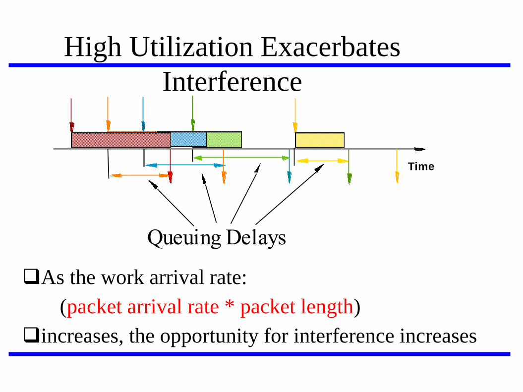
High Utilization Exacerbates

Interference

As the work arrival rate:

(packet arrival rate * packet length)‏

increases, the opportunity for interference increases

Time

Queuing Delays

Bottlenecks

Types of bottlenecks

At access points (flow control, prioritization, QoS

enforcement needed)‏

At points within the network core

Isolated (can be analyzed in isolation)‏

Interrelated (network or chain analysis needed)

Bottlenecks result from overloads caused by:

High load sessions, or

Convergence of sufficient number of moderate load

sessions at the same queue

Bottlenecks Cause Shaping

The departure traffic from a bottleneck is more regular than

the arrival traffic

The inter-departure time between two packets is at least as

large as the transmission time of the 2nd packet

Bottlenecks Cause Shaping

Bottleneck

90% utilization

Outgoing traffic Incoming traffic

Exponential

inter-arrivals

gap

Bottleneck

90% utilization

Outgoing traffic Incoming traffic

Large

Medium

Small

Variable packet sizes

Histogram of inter-departure times for small packets

sec

# of packets

Peaks smeared

Variable packet sizes

Constant packet sizes

21

Queuing Models

Widely used to estimate desired performance measures of the

system

Provide rough estimate of a performance measure

Typical measures

Server utilization

Length of waiting lines

Delays of customers

Applications

Determine the minimum number of servers needed at a

service centre

Detection of performance bottleneck or congestion

Evaluate alternative system designs

22

Kendall Notation

A/S/m/B/K/SD

A: arrival process

S: service time distribution

m: number of servers

B: number of buffers(system capacity)‏

K: population size

SD: service discipline

23

Service Time Distribution

Time each user spends at the terminal

IID

Distribution model Exponential

Erlang

Hyper-exponential

General

cf. Jobs = customers

Device = service centre = queue

Buffer = waiting position

24

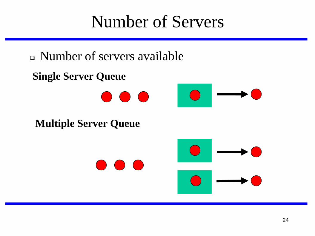
Number of Servers

Number of servers available

Single Server Queue

Multiple Server Queue

25

Service Disciplines

First-come-first-served(FCFS)‏

Last-come-first-served(LCFS)‏

Shortest processing time first(SPT)‏

Shortest remaining processing time first(SRPT)‏

Shortest expected processing time first(SEPT)‏

Shortest expected remaining processing time first(SERPT)‏

Biggest-in-first-served(BIFS)‏

Loudest-voice-first-served(LVFS)‏

26

Example

M/M/3/20/1500/FCFS

Time between successive arrivals is exponentially

distributed

Service times are exponentially distributed

Three servers

20 buffers = 3 service + 17 waiting

After 20, all arriving jobs are lost

Total of 1500 jobs that can be serviced

Service discipline is first-come-first-served

27

Default

Infinite buffer capacity

Infinite population size

FCFS service discipline

Example

G/G/1 G/G/1/

28

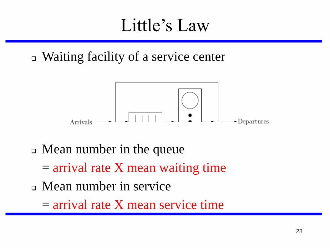
Little’s‏Law

Waiting facility of a service center

Mean number in the queue

= arrival rate X mean waiting time

Mean number in service

= arrival rate X mean service time

29

Example

A monitor on a disk server showed that the average time to

satisfy an I/O request was 100msecs. The I/O rate was about

100 request per second. What was the mean number of

request at the disk server?

Solution:

– Mean number in the disk server

= arrival rate X response time

= (100 request/sec) X (0.1 seconds)‏

= 10 requests

30

Stochastic Processes

Process : function of time

Stochastic process

process with random events that can be described by a

probability distribution function

A queuing system is characterized by three elements:

A stochastic input process

A stochastic service mechanism or process

A queuing discipline

31

Types of Stochastic Process

Discrete or continuous state process

Markov processes

Birth-death processes

Poisson processes Markov process

Birth-death process

Poisson process

32

Discrete/Continuous State Processes

Discrete = finite or countable

Discrete state process

Number of jobs in a system n(t) = 0,1,2,…

Continuous state process

Waiting time w(t)‏

Stochastic chain : discrete state stochastic process

33

Markov Processes

Future states are independent of the past

Markov chain : discrete state Markov process

Not necessary to know how log the process has been in the

current state

State time : memory less(exponential) distribution

M/M/m queues can be modelled using Markov processes

The time spent by a job in such a queue is a Markov process and

the number of jobs in the queue is a Markov chain

34

M/M/1 Queue

The most commonly used type of queue

Used to model single processor systems or individual devices in a computer system

Assumption

Interarrival rate of exponentially distributed

Service rate of exponentially distributed

Single server

FCFS

Unlimited queue lengths allowed

Infinite number of customers

Need to know only the mean arrival rate() and the mean service rate

State = number of jobs in the system*

35

M/M/1 Operating Characteristics

Utilization(fraction of time server is busy)‏

ρ = /

Average waiting times

W = 1/( - )

Wq = ρ/( - ) = ρ W

Average number waiting

L = /( - )

Lq = ρ /( - ) = ρ L

36

Flexibility/Utilization Trade-off

Utilization = 1.0 = 0.0

L Lq

W Wq

High utilization Low ops costs Low flexibility Poor service

Low utilization High ops costs High flexibility Good service

Must trade off benefits of high utilization levels with benefits

of flexibility and service

37

M/M/1 Example

On a network gateway, measurements show that the packets

arrive at a mean rate of 125 packets per seconds(pps) and the

gateway takes about two milliseconds to forward them. Using an

M/M/1 model, analyze the gateway. What is the probability of

buffer overflow if the gateway had only 13 buffers? How many

buffers do we need to keep packet loss below one packet per

million?

38

Arrival rate = 125pps

Service rate = 1/.002 = 500 pps

Gateway utilization ρ = / = 0.25

Probability of n packets in the gateway

(1- ρ) ρ n = 0.75(0.25)n

Mean number of packets in the gateway

ρ/(1- ρ) = 0.25/0.75 = 0.33

Mean time spent in the gateway

(1/ )/(1- ρ) = (1/500)/(1-0.25) = 2.66 milliseconds

Probability of buffer overflow

P(more than 13 packets in gateway) = ρ13 = 0.2313 =1.49 X 10-8 ≈ 15 packets per billion packets

To limit the probability of loss to less than 10-6

ρ n < 10-6

n > log(10-6)/log(0.25) = 9.96

Need about 10 buffers

39

Effects of congestion

Congestion occurs when number of packets

transmitted approaches network capacity

Objective of congestion control:

keep number of packets below level at

which performance drops off dramatically

40

Queuing Theory

Data network is a network of queues

If arrival rate > transmission rate

then queue size grows without bound and

packet delay goes to infinity

41

42

At Saturation Point, 2 Strategies

Discard any incoming packet if no buffer

available

Saturated node exercises flow control over

neighbours

May cause congestion to propagate throughout

network

43

Figure 10.2

44

Ideal Performance

i.e., infinite buffers, no overhead for packet

transmission or congestion control

Throughput increases with offered load until

full capacity

Packet delay increases with offered load

approaching infinity at full capacity

Power = throughput / delay

Higher throughput results in higher delay

45

Figure 10.3

46

Practical Performance

i.e., finite buffers, non-zero packet processing overhead

With no congestion control, increased load eventually causes moderate congestion: throughput increases at slower rate than load

Further increased load causes packet delays to increase and eventually throughput to drop to zero

47

Figure 10.4

48

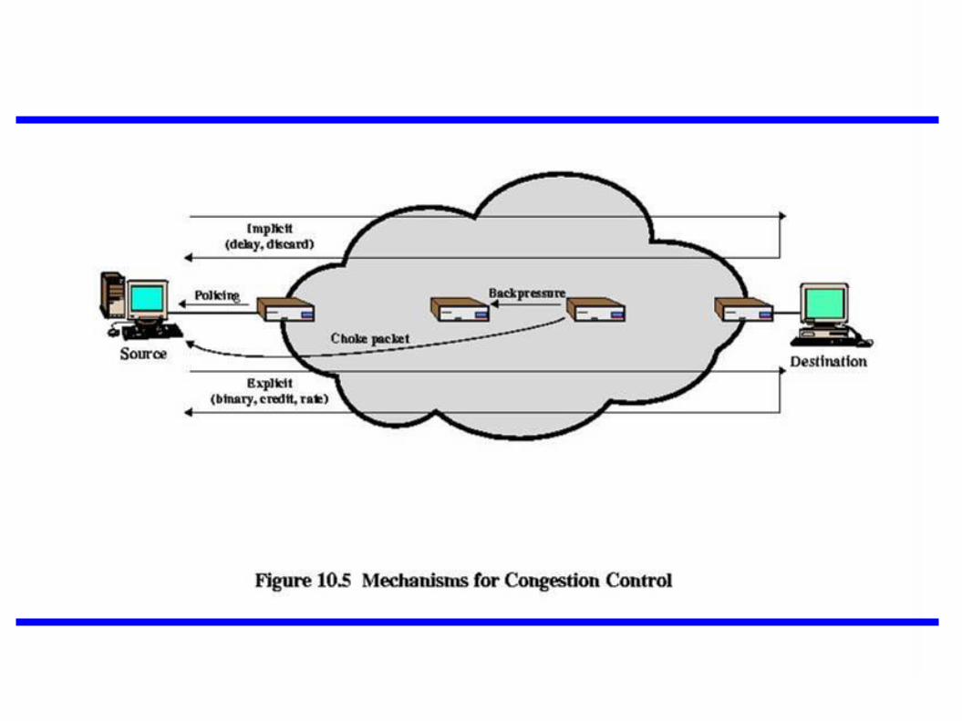
Congestion Control

Backpressure

Request from destination to source to reduce rate

Choke packet: ICMP Source Quench

Implicit congestion signaling

Source detects congestion from transmission

delays and discarded packets and reduces flow

49

Explicit congestion signaling

Direction

Backward

Forward

Categories

Binary

Credit-based

rate-based

50

Traffic Management

Fairness

Last-in-first-discarded may not be fair

Quality of Service

Voice, video: delay sensitive, loss insensitive

File transfer, mail: delay insensitive, loss sensitive

Interactive computing: delay and loss sensitive

Reservations

Policing: excess traffic discarded or handled on best-effort

basis

51

Figure 10.5

52

Frame Relay Congestion Control

Minimize frame size Maintain QoS Minimize monopolization of network Simple to implement, little overhead Minimal additional network traffic Resources distributed fairly Limit spread of congestion Operate effectively regardless of flow Have minimum impact other systems in network Minimize variance in QoS

53

54

Traffic Rate Management

Committed Information Rate (CIR)‏

Rate that network agrees to support

Aggregate of CIRs < capacity

For node and user-network interface (access)‏

Committed Burst Size

Maximum data over one interval agreed to by network

Excess Burst Size

Maximum data over one interval that network will attempt

55

56

Figure 10.7

57

Congestion Avoidance with Explicit Signaling

2 strategies

Congestion always occurred slowly, almost

always at egress nodes

forward explicit congestion avoidance

Congestion grew very quickly in internal nodes

and required quick action

backward explicit congestion avoidance

58

2 Bits for Explicit Signaling

Forward Explicit Congestion Notification

For traffic in same direction as received

frame

This frame has encountered congestion

Backward Explicit Congestion Notification

For traffic in opposite direction of received

frame

Frames transmitted may encounter

congestion

59

Questions ?