High Resolution Topology Design with Iso-XFEM

M. Abdi, I. Ashcroft, R. Wildman

Faculty of Engineering, The University of Nottingham, Nottingham NG7 2RD, UK

Abstract

Topology optimization, as a challenging aspect of structural optimization, has gained

interest in recent years as a method of designing structures to take advantage of the design

freedoms of advanced manufacturing techniques such as Additive Manufacturing (AM). The

majority of topology optimization algorithms are integrated with the Finite Element Method

(FEM) to enable the analysis of structures with complex geometry during the optimization

process. However, due to the finite element-based nature of the subsequent topology optimized

solutions, the design boundaries are dependent on the finite element mesh used and tend not to

have the desired smoothness for direct fabrication. The topology optimized solutions may,

therefore, need smoothing, reanalysing and shape optimization before they become

manufacturable. In this study, an Extended Finite Element Method (X-FEM) is employed and

integrated with an evolutionary structural optimization algorithm, aiming to avoid/decrease the

post-processing required from topology optimization design to manufacture. Rather than using

finite elements for boundary representation, an isoline/isosurface approach is used to capture the

design boundary during the optimization process. The comparison of the X-FEM-based solutions

with the FE-based ones for the topology optimization of test cases representing real industrial

components indicates significant improvements in the solutions’ boundary representation as well

as their structural performance.

Introduction

Additive manufacturing (AM) has grown over the last 30 years to be used in various

application areas. It contrasts with the conventional fabrication processes which are usually

subtractive or formative, in that the part is built up layer-by-layer. This layer manufacturing

approach allows producing parts of significantly greater complexity compared with traditional

processes and this increased complexity generally does not have a significant effect on the cost

of the process. Not only this provides the designer with significantly greater design freedom, it

also enables the built part to be closer to the optimum design than is possible with traditional

processes (Brackett et al 2011).

The level of freedom offered by AM processes necessitates the development of new

design tools since the current design tools were developed prior to AM and are therefore better

suited to traditional manufacturing methods. Topology optimization, however, offers great

potential for AM, since it is capable of achieving solutions with great complexity. Topology

optimization is a structural optimization technique, mainly developed in the last three decades,

which aims to find the best possible material distribution and connectivity for a structure within a

specified design domain under a set of loads and boundary conditions. It involves finding the

number of members required in the design and the manner in which these members are

1288

connected. There have been a significant number of papers dedicated to this subject mainly

based on homogenisation (Bendsøe and Kikuchi, 1988), Solid Isotropic Material with

Penalization (SIMP) (Bendsøe, 1989; Zhou and Rozvany, 1991), Evolutionary Structural

Optimization (ESO) (Xie and Steven 1993, 1997), level set method (Wang et al., 2003; Allaire et

al, 2004) and genetic algorithms (Jakiela et al. 2000; Ryoo and Hajela 2004). Most of the

proposed topology optimization algorithms have been applied to simple, standard problems, such

as Michelle-type structures and cantilever beams with rectangular domains, there has been less

attention on applying these algorithms to 3D real-life structures and loading scenarios. In some

cases the mathematical complexity or the size of the FE design domain doesn’t allow the

algorithm to be properly implemented. OptiStruct (Altair Engineering Inc.) is an example of

software designed to enable the SIMP method of topology optimization to be applied to real

components. Other software such as Nastran (MSC Software) and Abaqus FEA (Dassault

Systèmes) also have options to apply similar density-based approaches to find the solution to

topology optimization problems. Although the topology optimization modules of these software

applications are being widely used for research and engineering purposes, a drawback of the

density-based approaches (and many other element-based approaches) is that they cannot

provide a clear and smooth representation of the design boundaries in converged topologies. This

issue brings difficulties in interpreting the solutions, combining them with CAD and

manufacturing the topologies. Therefore the solutions usually need post-processing, reanalysing

and shape optimization before manufacture, which is costly and time consuming.

A possible alternative approach to the conventional element-based methods in topology

optimization is the use of the eXtended Finite Element Method (X-FEM) combined with an

implicit representation of the design boundaries (such as those in level set and isoline/isosurface

approaches). X-FEM extends the classical finite element approach by adding special shape

functions which can represent a discontinuity inside finite elements. Therefore in structural

optimization applications, X-FEM can be used where the boundary of the design crosses finite

elements, without the need to remesh the boundaries. In the isoline approach (Maute and Ramm,

1995; Lee et al, 2007; Victoria et al, 2009) the boundary of a design is represented by isolines of

a selected measure of structural performance behaviour, such as von Mises stress or strain energy

density. In a previous study (Abdi et al 2014a), an evolutionary based optimization approach

combined with X-FEM and isoline boundary representation was used for the topology

optimization of 2D continuum domains. The numerical comparison of the converged solutions

from Iso-XFEM approach with those obtained using bi-directional evolutionary structural

optimization (BESO) showed the efficiency of the algorithm. The aim of this paper is to extend

the Iso-XFEM method into 3D to address the application of X-FEM and isolines/isosurfaces of

structural performance to the topology optimization of real-life structures. To meet this aim, 2D

and 3D test cases including an industrial arm are considered and a comparison of the solutions

with BESO (as a discrete element-based topology optimization method) solutions is presented.

Isoline and Isosurface Boundary Representation

In general, isoline/isosurfaces are the lines/surfaces that represent the points of a constant

value, named the isovalue, in a 2D/3D space. The isoline approach is an implicit method of

defining the boundaries of a design in a 2D fixed grid design domain. In this approach the

boundaries are defined using the contours of a higher dimension (3D) of structural performance,

1289

such as Strain Energy Density (SED) or von Mises stress, obtained from finite element analysis

of the design space. The isosurface approach is the extension of the isoline method to the

representation of the boundaries of a 3D design using contours of a 4D structural performance. In

structural optimization applications (Victoria et al 2009, 2010; Abdi et al 2014a, 2014b) the

boundaries are defined by the intersection of the structural performance (SP) distribution with a

minimum level of performance (MLP), which is typically increasing during the optimization

process. Figure 1 shows a 2D fixed grid design domain discretized with a 30x30 mesh, where the

intersection of the SED distribution as a structural performance criteria with a minimum level of

SED gives the design boundary.

The regions of the design domain in which the structural performance is lower than the

MLP is defined as the void part of the domain and those which have a higher value than the MLP

form the solid part of the design domain. The relative performance, , is defined as:

(1)

Following this, the design domain can be partitioned into void phase, boundary and solid phase,

with respect to the values of relative performance, as

( ) {

( ) ( ) ( )

(2)

Figure 2 shows how the design space, D, from figure 1 is partitioned into , and

using the relative performance function ( ), distributed over the design space.

Figure 1. Design boundary represented by intersection of a SP with the MLP.

1290

Figure 2. A 2D design domain represented by its relative structural performance. (a) Relative

performance model. (b) Design domain.

By implementing the above isoline/isosurface approach, the design boundary is

superimposed on the fixed grid finite elements, making three groups of elements in the FE design

space: solid elements, void elements, and boundary elements (the elements which lie on the

boundary) as demonstrated in figure 3. The contribution of solid and void elements to the FE

framework could simply be considered using a soft-kill scheme (Huang and Xie, 2009) in which

instead of deleting the elements in the void phase, they are assigned a weak material property.

However, in order to accurately represent the design boundary whilst avoiding expensive

remeshing operations, an X-FEM approach can be employed as discussed in the next section.

Figure 3. The elements are classified into 3 groups by superimposing the design geometry on the

fixed grid FE mesh.

X-FEM for Structural Optimization

X-FEM (Belytschko and Black, 1999; Moës et al, 1999) is a generalized approach for the

classical finite element method which can represent discontinuities such as cracks, holes,

inclusions, and fluid/structure interaction, inside finite elements without the need to remesh the

internal boundaries. In the X-FEM, the classical finite element (FE) shape functions are extended

by adding discontinuous shape functions to the displacement field in order to enrich the FE

approximation space near the discontinuity. X-FEM has been applied to various kinds of

discontinuity by defining an enrichment function appropriate to the nature of the discontinuity. In

the case of structural optimization problems, X-FEM can be implemented to represent the

1291

evolving boundary of a design on a fixed grid FE mesh with no need for remeshing. In this case

the elements which lie on the design boundary experience a material-void discontinuity. In this

case, the X-FEM scheme for modelling holes and inclusions proposed by Sukumar et al (2001)

can be utilized to represent the FE approximation space near the discontinuity:

( ) ∑ ( ) ( ) (3)

where are the classical FE shape functions, are the nodal degrees of freedom and H(x) is a

Heaviside function with the following properties

( ) {

(4)

implying that the value of the Heaviside function switches from 1 to 0 in the void parts of the

design domain. In order to realize the above X-FEM scheme, integration over the element

domains are only performed on the solid sub-domain of the boundary elements while the fully

solid/void elements are treated using the conventional FEM. Following this, the stiffness matrix

of a 2D element can be defined by

∫ ( )

(5)

where is the element domain, is the displacement differentiation matrix, is the elasticity

matrix for the solid material and t is the thickness of the element.

Various partitioning schemes can be implemented to realize the above X-FEM integration

scheme, dependent to the element type that is used in the FE model of the domain of interest. In

the case of 2D quad elements, we can partition the solid sub-domain of the elements into sub-

triangles and use the Gauss quadrature method to numerically calculate the integral for each

triangle. The element stiffness matrix can then be obtained by summing the contributions of each

sub-triangle (figure 4).

Figure 4. Quadrilateral boundary elements represented by the 2D X-FEM scheme.

1292

Figure 5. Decomposing a boundary hexahedral element: (a) a boundary hexahedral element

where the whole element domain is partitioned into 24 sub-tetrahedra; (b) a solid sub-

tetrahedron; (c) a boundary sub-tetrahedron where the solid sub-domain is further partitioned

into sub-tetrahedrons.

In the case of 3D Hex elements, the solid sub-domain of the boundary elements are

partitioned into sub-tetrahedrons and the integration is numerically performed over the solid

tetrahedrons. In our implementation, the hexahedral boundary element is initially partitioned into

24 sub-tetrahedra by dividing each of the 6 surfaces of the element into 4 triangles and

connecting the edges of the triangles to the centroid of the hexahedron. The void tetrahedra are

then removed from the integration domain. The bi-material (solid/void) tetrahedra are again

partitioned into smaller sub-tetrahedra and the void tetrahedra removed from the integration

domain. Integration is eventually performed over the remaining solid tetrahedra (figure 5).

Evolutionary based Optimization Algorithm using Isolines/Isosurfaces

The optimization algorithm developed in this study is evolutionary based, i.e. based on the

simple assumption that the optimized solution can be achieved by gradually removing the

inefficient material from the design domain. Examples of evolutionary based optimization

methods include ESO in which inefficient elements are gradually removed throughout the

optimization process, and BESO in which the elements are added and removed simultaneously

throughout the process. However, unlike ESO and BESO in which the material removal/addition

is carried out at an elemental level, in this approach the optimization operates at a global level of

structural performance by the use of isoline/isosurface design representation. An appropriate

performance criterion is used to characterize the efficiency of material usage in the design

domain. Material is then removed from low relative performance regions ( ( ) ) and

redistributed to the high relative performance regions ( ( ) ). As shown in equation 1,

the relative performance can be calculated by subtracting a minimum level of performance

(MLP) from the structural performance (SP). However, in order to stabilize the evolutionary

1293

process, as suggested by Huang and Xie (2007), historical information of the structural

performance can be used by averaging the current relative performance with that from the

previous iteration:

Figure 6. Flowchart of the optimization method.

(6)

where i denotes the node number and it is the current iteration number. The minimum level of

performance (MLP) which is used in equation 1 to find the relative performance, is usually

increasing during the evolutionary process and can be calculated from:

/ (7)

where is the maximum performance over the design domain and is the redistribution

factor for the current iteration. is the current volume fraction of the solid material to the

whole domain, and is used in the above equation to accelerate the material removal process at

lower volume fractions. With the current redistribution factor, the iterative process of the

1294

extended finite element analysis and material removal/redistribution takes place until the

percentage change in volume fraction is less than a minimum value , which means that a

steady state is almost reached. Then, the redistribution factor is increased by adding an

evolutionary rate, ER:

. (8)

With the new redistribution factor, the extended finite element analysis and material

removal/redistribution is repeated until a new steady state is reached. The evolutionary process

continues until a desired optimum, such as a final volume fraction ( ) is reached. Figure 6

summarizes the optimization algorithm used in this study.

Test Cases

In order to illustrate the efficiency of the proposed Iso-XFEM algorithm, 2D and 3D test

cases are presented in this section. A Matlab code was developed to apply the Iso-XFEM

algorithm. The design domains of the test cases were more complex than the test cases used in

the previous study (Abdi et al, 2013), and the mesh was not necessarily structured in these cases.

Also, in the 3D test case, a non-design domain was considered which is usually the case in the

topology optimization of real structures. Therefore, due to the complexity of the initial

geometries, the FE models of the structures were created in a FE package and then imported into

Matlab in terms of Nodes and Elements matrices. All the results were generated using a desktop

computer with an Intel Xeon 2 processor of 2.4 GHz speed and 24 GB RAM.

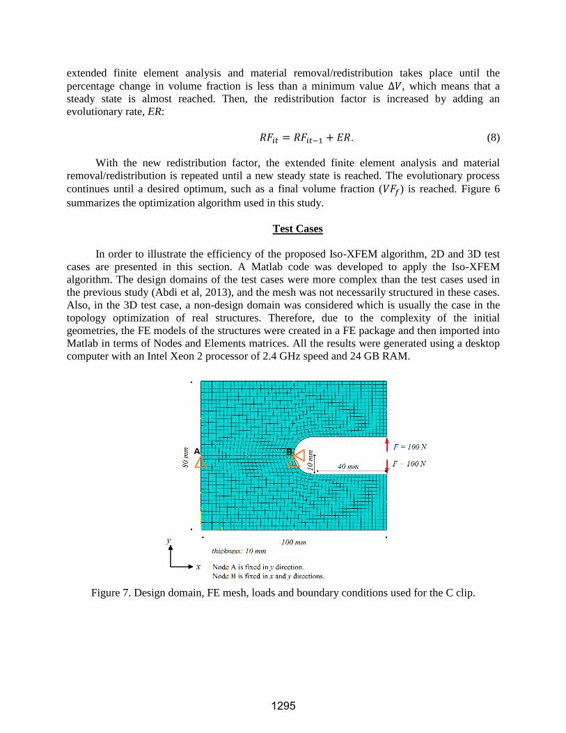
Figure 7. Design domain, FE mesh, loads and boundary conditions used for the C clip.

1295

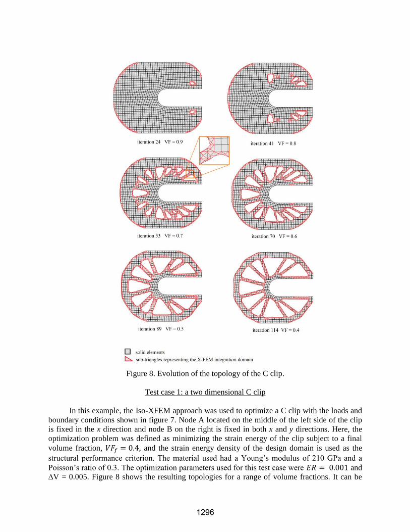
Figure 8. Evolution of the topology of the C clip.

Test case 1: a two dimensional C clip

In this example, the Iso-XFEM approach was used to optimize a C clip with the loads and

boundary conditions shown in figure 7. Node A located on the middle of the left side of the clip

is fixed in the x direction and node B on the right is fixed in both x and y directions. Here, the

optimization problem was defined as minimizing the strain energy of the clip subject to a final

volume fraction, , and the strain energy density of the design domain is used as the

structural performance criterion. The material used had a Young’s modulus of 210 GPa and a

Poisson’s ratio of 0.3. The optimization parameters used for this test case were and

∆V = 0.005. Figure 8 shows the resulting topologies for a range of volume fractions. It can be

1296

seen that the process of material removal was carried out by creating a number of holes in the

low SED regions of the design space, followed by the merging and enlarging of holes until the

desired volume fraction and convergence conditions were achieved. The triangles near the

boundary represent the X-FEM integration domains and are not elements. Therefore as no

element is added or removed to/from the design domain, the number of degrees of freedom

during the optimization process hasn’t been changed. However, the boundary of the converged

solution (figure 9) is smoothly defined by implementing the isoline and X-FEM approaches. The

optimization converged after 120 evolutionary iterations which took 170 seconds.

Figure 9. Converged solution for VF = 0.4 at iteration 120.

Test case 2: an industrial arm

In order to implement the Iso-XFEM topology optimization method on a practical

problem, the industrial arm shown in figure 10 which was previously studied using BESO

(Aremu et al, 2013), was considered. A load of 667.23 N was uniformly distributed on the lower

edge of surface A, and all degrees of freedom on surface B were fixed, forming a cantilever

beam. Two levels of difficulty existed in this problem compared to the 2D/3D cantilever

problems often used in the literature; an increasing geometrical complexity and existence of non-

design domain. The grey cylindrical regions in figure 10 were set as non-design domain and the

rest of the structure was the design domain. The objective was to minimize the total strain energy

subject to a final volume fraction of 15% of the design domain. The material properties of the

arm were a Young’s modulus E =74 GPa and Poisson’s ratio υ = 0.33. Two experiments

employing different mesh sizes were considered for this test case. In each of the experiments, the

optimized solution was obtained using the proposed Iso-XFEM approach and the element-based

BESO method. This was to enable the effectiveness and efficiency of the two approaches to be

compared.

Experiment 1

The whole domain was meshed using approximately 22000 hexahedral elements. The

optimization parameters were and . The resulting topologies obtained

using the Iso-XFEM method for a range of volume fractions up to 0.15 are shown in figure 11.

Employing the same mesh used for the previous experiment, the topology optimization problem

1297

of the arm was solved using a soft-kill BESO code based on Huang and Xie’s study (2007). The

BESO parameters used were an evolution rate, ER = 0.02, and sensitivity filter radius of 1.2

times the average element size. The converged solutions of the two approaches are shown in

figure 12.

Figure 10. Design domain and non-design domain of the industrial arm.

Figure 11. Evolution of the topology of the industrial arm.

1298

Figure 12. Converged solutions of experiment 1: (a) Iso-XFEM solution and (b) BESO solution

for VF = 0.15. Surface roughness was measured in regions Z1 and Z2.

Figure 13. Converged solutions in experiment 2: (a) Iso-XFEM solution and (b) BESO solution

for VF = 0.15.

1299

Experiment 2

In this experiment, the whole domain of the industrial arm was discretised using

approximately 32000 Hex elements. The topology optimization of the arm was considered using

both the BESO and Iso-XFEM optimization approaches with the same optimization parameters

as were used in experiment 1. Figure 13 shows the converged solutions obtained using the two

different approaches. It can be seen that the converged solutions in experiment 2 have similar

topologies to those seen in experiment 1 (figure 12), apart from the fact that topologies with

more members have been realized by using the finer mesh in experiment 2 (table 1).

Discussion

Considering experiment 1, it can be seen that both Iso-X-FEM and BESO approaches have

successfully obtained converged solutions for the topology optimization problem of the

industrial arm as an example of a real structure. It can be seen that the overall topologies of the

converged solutions look similar; however the Iso- XFEM solution has a much smoother surface

than the BESO solution. Measuring the surface roughness of the solutions is not very easy as it

varies depending on the geometrical features forming the topology. Assuming that spherical and

cylindrical features have higher values of surface roughness than flat features, two regions Z1

(hemispherical) and Z2 (cylindrical) in figure 12 for experiment 1 (and similar regions in figure

13 for experiment 2) were considered and their arithmetic mean surface roughness, , was

calculated, as shown in table 1. It can be seen that in both regions, much higher values of surface

roughness are obtained with the BESO solution. The jagged edges of the coarse finite elements

on the boundary of the BESO solution (figure 12b) has resulted in an unfeasible design boundary

which needs further interpretation of the topology and post processing such as smoothing,

reanalysing and shape optimization before manufacture. Comparing the strain energies of the

BESO and Iso-XFEM solutions in table 1, it can be seen that the Iso-XFEM approach has

resulted in a performance for the converged solution approximately 18% higher than the BESO

solution when compared with the same mesh size. It can also be seen that the BESO solution has

fewer members (less complexity) than the Iso-XFEM solution (tale 1). A reason for this could be

the sensitivity filtering scheme (Sigmond and Peterson, 1998) that is employed with the BESO

method (and many other element-based methods). This scheme is used to eliminate checkerboard

pattern problems, however this filtration scheme is not required for the proposed Iso-XFEM

method, although it can be used if solutions with less complexity are desired.

Comparing the time cost of the two optimization approaches in experiment 1 (table 1), one

may notice that the Iso-XFEM optimization approach operates slower than the BESO method for

the same initial mesh as it takes more time to calculate the properties of boundary elements using

the X-FEM integration scheme. However the time spent to solve the finite element linear system

of equations will be approximately the same, as the same number of degrees of freedom exists in

the both methods. Therefore it is expected that by increasing the mesh density which results in

increasing the number of degrees of freedom, the percentage difference between the solution

time of the two approaches decreases. This issue was investigated by performing experiment 2 in

which the design domain is discretised with a finer mesh than experiment 1.

1300

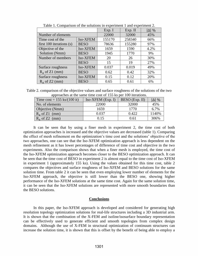
Table 1. Comparison of the solutions in experiment 1 and experiment 2.

Exp. I Exp. II | |

Number of elements 22000 32000 45%

Time cost of the

first 100 iterations (s)

Iso-XFEM 155170 258340 66%

BESO 78636 155280 97%

Objective of the

Solution (Nmm)

Iso-XFEM 1659 1590 4.2%

BESO 1945 1770 9%

Number of members Iso-XFEM 20 26 30%

BESO 15 19 27%

Surface roughness

of Z1 (mm)

Iso-XFEM 0.037 0.019 49%

BESO 0.62 0.42 32%

Surface roughness

of Z2 (mm)

Iso-XFEM 0.15 0.12 20%

BESO 0.65 0.61 6%

Table 2. comparison of the objective values and surface roughness of the solutions of the two

approaches at the same time cost of 155 ks per 100 iterations.

Time cost = 155 ks/(100 it) Iso-XFEM (Exp. I) BESO (Exp. II) | |

No. of elements 22000 32000 45%

Objective (Nmm) 1659 1770 6.7%

of Z1 (mm) 0.037 0.422 1140%

of Z2 (mm) 0.15 0.61 306%

It can be seen that by using a finer mesh in experiment 2, the time cost of both

optimization approaches is increased and the objective values are decreased (table 1). Comparing

the effect of mesh refinement on the optimization’s time cost and the solutions’ objective of the

two approaches, one can see that the Iso-XFEM optimization approach is less dependent on the

mesh refinement as it has lower percentages of difference of time cost and objective in the two

experiments. Also the comparison shows that when a finer mesh is employed, the time cost of

the Iso-XFEM optimization approach becomes closer to the BESO optimization approach. It can

be seen that the time cost of BESO in experiment 2 is almost equal to the time cost of Iso-XFEM

in experiment 1 (approximately 155 ks). Using the values obtained for this time cost, table 2

compares the objectives and surface roughness of Iso-XFEM and BESO solutions for the same

solution time. From table 2 it can be seen that even employing lower number of elements for the

Iso-XFEM approach, the objective is still lower than the BESO one, showing higher

performance of the Iso-XFEM solutions at the same time cost. Again for the same solution time,

it can be seen that the Iso-XFEM solutions are represented with more smooth boundaries than

the BESO solutions.

Conclusions

In this paper, the Iso-XFEM approach is developed and considered for generating high

resolution topology optimization solutions for real-life structures including a 3D industrial arm.

It is shown that the combination of the X-FEM and isoline/isosurface boundary representation

can be effectively used to generate efficient and smooth topologies from complex design

domains. Although the use of X-FEM in structural optimization of continuum structures can

increase the solution time, it is shown that this is offset by the benefit of being able to employ a

1301

coarse mesh to generate a smooth topology. Therefore, not only are the structural performances

of the final solutions higher than the solutions obtained from an evolutionary element-based

method like BESO, the total time that is required to present a solution with clearly defined

boundaries can be reduced.

Acknowledgements

The authors are grateful for the funding provided by the University of Nottingham.

References

Abdi, M., Wildman, R., Ashcroft, I. (2014a). Evolutionary topology optimization using extended finite element

method and isolines. Engineering Optimization, 46(5), 628-647.

Abdi, M., Ashcroft, I., Wildman, R. (2014b). An X-FEM based approach for topology optimization of continuum

structures. Advances in Intelligent Systems and Computing, 256, 277-289.

Allaire, G., Jouve, F., Toader, A. M. (2004). Structural optimisation using sensitivity analysis and a level set

method, J. Comp. Phys., 194, 363-393.

Aremu, A., Ashcroft, I., Wildman, R, Hague, R., Tuck, C., Brackett, D. (2013). The effects of bidirectional

evolutionary structural optimization parameters on an industrial designed component for additive manufacture.

Proc IMechE Part B: J Engineering Manufacture, 227(6), 794-807.

Bendsøe, M.P. (1989). Optimal shape design as a material distribution problem. Struct. Optim. 1, 193-202.

Bendsøe, M.P. and Kikuchi, N. (1988). Generating optimal topologies in structural design using a homogenization

method. Computer Methods in Applied Mechanics and Engineering, 71, 197-224.

Belytschko, T. and Black, T. (1999). Elastic crack growth in finite elements with minimal remeshing. International

Journal for Numerical Methods in Engineering, 45 (5), 601-620.

Brackett, D., Ashcroft, I., Hague, R. (2011). Topology optimization for additive manufacturing. Proceedings of the

24th Solid Freeform Fabrication Symposium (SFF2011), 348-362.

Daux, C., Moës, N., Dolbow, J., Sukumar, N., Belytschko, T. (2000). Arbitrary cracks and holes with the extended

finite element method. Int. J. Numer. Methods Engrg., 48 (12), 1741-1760.

Huang, X., Xie, Y. M. (2009). Evolutionary Topology Optimisation of Continuum Structures, Wiley.

Huang, X. and Xie, Y.M. (2007). Convergent and mesh-independent solutions for bi-directional evolutionary

structural optimization method. Finite Elem Anal Des, 43, 1039-1049.

Jakiela, M., Chapman, C., Duda, J., Adewuya, A., Saitou, K. (2000). Continuum structural topology design with

genetic algorithms. Comput Methods Appl Mech Eng, 186(2–4), 339-356.

Lee, D., Park, S., Shin, S., (2007). Node-wise topological shape optimum design for structural reinforced modeling

of Michell-type concrete deep beams. J Solid Mech Mater Eng, 1(9), 1085-96.

Li, L., Wang, M.Y., Wei, P. (2012). XFEM schemes for level set based structural optimization. Front. Mech. Eng.,

7(4), 335–356.

Maute, K., Ramm, E. (1995). Adaptive topology optimisation. Struct Optim, 10, 100-12.

1302

Moës, N., Dolbow, J. and Belytschko, T. (1999). A finite element method for crack growth without remeshing,

International Journal for Numerical Methods in Engineering. 46, 131-150.

Ryoo, J., Hajela, P. (2004). Handling variable string lengths in GA-based structural topology optimization. Struct

Multidisc Optim, 26, 318-325.

Sigmund, O. and Petersson, J. (1998). Numerical instabilities in topology optimization: A survey on procedures

dealing with checkerboards, mesh-dependencies and local minima. Struct. Optim. 16, 68-75.

Sukumar, N., Chopp, D. L., Moës, N. and Belytschko, T. (2001). Modeling Holes and Inclusions by Level Sets in

the Extended Finite Element Method. Computer Methods in Applied Mechanics and Engineering, 190, 6183-6200.

Victoria, M., Martı´, P., Querin, O.M. (2009). Topology design of two-dimensional continuum structures using

isolines. Computer and Structures, 87, 101-109.

Victoria, M., Querin, O.M., Martı´, P. (2010). Topology design for multiple loading conditions of continuum

structures using isolines and isosurfaces. Finite Elements in Analysis and Design, 46, 229-237.

Wang, M.Y., Wang, X., Guo, D. (2003). A level set method for structural topology optimisation. Comput. Meth

.Appl. Eng., 192, 227-46.

Wei, P., Wang, M.Y., Xing, X. (2010). A study on X-FEM in continuum structural optimization using level set

method. Computer-Aided Design, 42, 708-719.

Xie, Y. M. and Steven, G.P. (1997). Evolutionary structural optimization, London.

Xie, Y. M. and Steven, G.P. (1993). A simple evolutionary procedure for structural optimization. Computers &

Structures, 49, 885-896

Zhou, M., Rozvany, G.I.N. (1991). The COG algorithm, Part II: Topological, geometrical and general shape

optimisation. Comp. Meth. Appl. Mech. Eng., 89, 309-336.

1303