high resolution differential laser interferometry for the
TRANSCRIPT

Université de Neuchâtel
Institut de Microtechnique
High Resolution Differential LaserInterferometry for the VLTI
(Very Large Telescope Interferometer)
èse
présentée à la Faculté des sciencespour obtenir le grade de docteur ès sciences
par
Olivier Scherler
Acceptée sur proposition du jury :Prof. René Dändliker, directeur de thèse
Prof. Hans Peter Herzig, Prof. éo Lasser,Prof. Yves Salvadé, Dr. Samuel Lévèque, rapporteurs.
Soutenue le 28 juin 2006

ii


iv

v
Space is big. Really big. You just won’t believe how vastly hugelymindbogglingly big it is. I mean you may think it’s a long way down theroad to the chemist, but that’s just peanuts to space.
(e Hitchhiker’s Guide to the Galaxy)

vi

vii
Abstract
One method for locating extrasolar planets is to observe the lateral movement of a starin the sky caused by a planet in orbit around it. In order to detect this displacement,the angular position of the star has to be measured with high accuracy. is techniqueis called astrometry.
e Very Large Telescope Interferometer (VLTI) is operated by the European South-ern Observatory and located at the Paranal Observatory in Chile. e purpose of thePRIMA instrument (Phase Referenced Imaging and Micro-arcsecond Astrometry) ofthe VLTI is to perform high-resolution astrometric measurements and high-resolutionimaging of faint stars using white light interferometry, by combining the light collectedby two telescopes. In order to allow the detection of extrasolar planets, the astrometricmeasurement has to be performed with micro-arcsecond accuracy.
In astrometric mode the PRIMA instrument observes two targets at the same time: theobject of scientific interest, and a bright reference star. e angular position of the scienceobject relative to the reference star is obtained by monitoring the differential optical pathtravelled by the light of each object in two separate white-light interferometers.
e aim of this work was to develop a high-resolution laser metrology based on super-heterodyne interferometry, with an accuracy of 5 nm over a differential optical path of100mm. Moreover the laser source had to be stabilised on an absolute frequency refer-ence, in order to ensure the long-term stability and calibration required to achieve thetarget performance. Superheterodyne interferometry allowed the direct measurementof the differential optical path using two heterodyne interferometers working with twodifferent frequency shifts. e differential phase measurement between the two inter-ferometers was obtained by electronic mixing of the two heterodyne signals, leading tothe differential optical path needed for the astrometric measurement.
Keywords: Metrology, Interferometry, Superheterodyne Detection, Laser Stabilisation,Very Large Telescope Interferometer.

viii

Contents
1 Introduction 1
2 e Very Large Telescope Interferometer 5
2.1 Principle of the PRIMA instrument . . . . . . . . . . . . . . . . . . 5
2.2 Requirements for the laser metrology . . . . . . . . . . . . . . . . . 8
2.3 Concept of the PRIMA laser metrology . . . . . . . . . . . . . . . . 9
2.4 Summary of the requirements for the PRIMA metrology . . . . . . . 14
3 Digital phasemeter for superheterodyne detection 15
3.1 Superheterodyne detection . . . . . . . . . . . . . . . . . . . . . . . 15
3.1.1 Frequency shifter module . . . . . . . . . . . . . . . . . . . 15
3.1.2 Electronic signal processing . . . . . . . . . . . . . . . . . . 17
3.2 Digital phase measurement . . . . . . . . . . . . . . . . . . . . . . 21
3.2.1 Phase-locked loop . . . . . . . . . . . . . . . . . . . . . . . 21
3.2.2 Digital zero-crossing phasemeter . . . . . . . . . . . . . . . 22
3.2.3 Averaging of phase data . . . . . . . . . . . . . . . . . . . . 27
3.2.4 Error compensation fringe counter . . . . . . . . . . . . . . 28
3.2.5 Status registers . . . . . . . . . . . . . . . . . . . . . . . . . 29
3.2.6 Data transfer . . . . . . . . . . . . . . . . . . . . . . . . . 30
ix

x Contents
4 Frequency stabilisation of a Nd:YAG laser 31
4.1 Frequency noise of the laser . . . . . . . . . . . . . . . . . . . . . . 31
4.1.1 Measurement of the beat frequency . . . . . . . . . . . . . . 31
4.1.2 Measurements at large OPD . . . . . . . . . . . . . . . . . . 32
4.1.3 Required frequency noise spectrum . . . . . . . . . . . . . . 35
4.2 Absolute stabilisation . . . . . . . . . . . . . . . . . . . . . . . . . 36
4.2.1 Absolute frequency references . . . . . . . . . . . . . . . . . 36
4.2.2 Stabilisation of the second-harmonic wavelength on iodine . . 37
4.2.3 Centre-of-fringe locking . . . . . . . . . . . . . . . . . . . . 37
4.3 Second-harmonic generation . . . . . . . . . . . . . . . . . . . . . . 40
4.3.1 Birefringent phase matching . . . . . . . . . . . . . . . . . . 40
4.3.2 Conversion efficiency . . . . . . . . . . . . . . . . . . . . . 41
4.3.3 Birefringent walk-off . . . . . . . . . . . . . . . . . . . . . 45
4.3.4 Quasi-phase matching in periodically-poled crystals . . . . . . 47
4.4 Set-up for the laser stabilisation . . . . . . . . . . . . . . . . . . . . 48
4.4.1 Second harmonic generation . . . . . . . . . . . . . . . . . 49
4.4.2 Frequency modulation . . . . . . . . . . . . . . . . . . . . 49
4.4.3 Absorption . . . . . . . . . . . . . . . . . . . . . . . . . . 50
4.4.4 Optical detection . . . . . . . . . . . . . . . . . . . . . . . 50
4.4.5 Control loop . . . . . . . . . . . . . . . . . . . . . . . . . 51
5 Tests of the phasemeter and of the laser stabilisation 53
5.1 Tests of the phasemeter . . . . . . . . . . . . . . . . . . . . . . . . 53
5.1.1 Electrical tests of the phasemeter . . . . . . . . . . . . . . . 53
5.1.2 Test of accuracy using two-wavelength interferometry . . . . . 57
5.1.3 Dynamic tests . . . . . . . . . . . . . . . . . . . . . . . . . 59
5.2 Tests of the laser stabilisation . . . . . . . . . . . . . . . . . . . . . . 64
5.2.1 Characterisation of the iodine cell . . . . . . . . . . . . . . . 64
xi
5.2.2 Error signal monitoring . . . . . . . . . . . . . . . . . . . . 67
5.2.3 Test with long delay lines . . . . . . . . . . . . . . . . . . . 68
5.2.4 Further tests performed at ESO . . . . . . . . . . . . . . . . 69
6 Conclusion 73
Acknowledgements 77
Bibliography 79

xii Contents

Chapter 1
Introduction
e Very Large Telescope Interferometer (VLTI), operated by the European SouthernObservatory and located at the Paranal Observatory in Chile, generates interferencefringes by combining the light collected by two telescopes observing a single object.e PRIMA instrument of the VLTI [1, 2] aims to perform high-resolution astrometricmeasurements and phase-referenced imaging by observing the interference fringes oftwo objects at the same time and by monitoring the optical path travelled by the light inthese two interferometers. e objective of this instrument is the detection of extra-solarplanets as well as high-resolution imaging of faint stars.
For these measurements, the knowledge of the differential optical path between the twostellar interferometers is needed. Superheterodyne detection was therefore proposed forthis purpose.
Superheterodyne detection was developed for two-wavelength interferometry by Dänd-liker et al. [3]. In two-wavelength interferometry, a synthetic wavelength Λ is generatedfrom two individual wavelengths λ1 and λ2 and can be chosen to be much longer thanthe optical wavelengths. Measurement of the phase at the synthetic wavelength allowsone to reduce the sensitivity or to extend the range of unambiguity for interferometricmeasurements.
Superheterodyne detection uses two different heterodyne frequencies f1 and f2 for theindividual wavelengths λ1 and λ2 to permit high-resolution phase measurements at thesynthetic wavelength without optical separation of the individual wavelengths. By feed-ing the two heterodyne signals to an electronic mixer, it is possible to measure the phase
1

2 Chapter 1. Introduction
difference directly. For the VLTI, superheterodyne detection is not used to measure asingle optical path with two different wavelengths (as originally intended), but to meas-ure two distinct optical paths with a single wavelength.
e present work is the result of a collaboration between IMT (Institute ofMicrotechno-logy, Neuchâtel) and ESO (European Southern Observatory, Garching bei München).It was supported by the FINES program of the Swiss National Science Foundation.
e goal of this work was to develop a high-resolution laser metrology based on super-heterodyne interferometry, capable of measuring the differential optical path betweentwo distinct interferometers with 5 nm accuracy, without having to take two separatephase measurements and compute their difference. Moreover, the laser source had to bestabilised on an absolute frequency reference in order to ensure the long-term stabilityand calibration required to achieve the target resolution of 1 nm over 100mm.
Part of this work has already been published or presented at international conferences:
[A] S. Lévêque, Y. Salvadé, O. Scherler and R. Dändliker, “High accuracy laser met-rology enhances the VLTI,” Laser Focus World 38 (4), 101–104 (2002).
[B] S. A. Lévêque, R. Wilhelm, Y. Salvadé, O. Scherler and R. Dändliker, “Towardnanometer accuracy laser metrology for phase-referenced interferometry with theVLTI,” inW. A. Traub, ed., “Interferometry forOptical Astronomy II,” vol. 4838,pp. 983–994, SPIE (2003)
e principle of the PRIMA instrument of the VLTI is described in chapter 2. eneed for a high-accuracy laser metrology is explained and the specifications are derivedfrom the expected performance of PRIMA. e underlying concepts of heterodyne andsuperheterodyne interferometry are then presented.
Chapter 3 describes the optics and analogue electronics that were designed to implementsuperheterodyne detection, as well as the digital electronics that were built to performthe phase measurement. Emphasis has been put on the critical points that had to beaddressed in order to meet the specifications.
e frequency stabilisation of the metrology laser is presented in chapter 4. First, themeasurements of the frequency noise of the laser are discussed. e concept that wasselected for the stabilisation is then explained, including a discussion pertaining to thegeneration of the second harmonic of the laser. Finally, the stabilisation set-up is de-scribed.

3
Chapter 5 summarises all the tests that were performed on the digital phasemeter andon the stabilised laser in order to verify their performance. Finally, in-situ modificationsand tests of the stability of the laser are presented.

4 Chapter 1. Introduction

Chapter 2
e Very Large TelescopeInterferometer
2.1 Principle of the PRIMA instrument
e Very Large Telescope (VLT), located at the Paranal Observatory in Chile comprisesfour fixed unit telescopes (UT) of 8.2m diameter and four movable auxiliary telescopes(AT) of 1.8m diameter that can be positioned over thirty different stations. e VLToperating in interferometric mode is called the Very Large Telescope Interferometer(VLTI). In this mode, two telescopes are used at the same time to form a stellar in-terferometer.
e VLTI generates interference fringes from a stellar object by combining the lightcollected by two telescopes distant by several meters. Since the object is a wide spectrumsource, delay lines operating between the telescopes and the interferometric laboratoryare used to equal the optical paths followed by the stellar light through each telescope,making the interference possible. Observation of the interference fringes then allows thereconstruction of an image of the object with an increased resolution compared to thatof a single telescope.
e PRIMA instrument (Phase Referenced Imaging and Micro-arcsecond Astrometry)aims to improve the performance of the VLTI by observing at the same time as theobject of interest (science object) a bright reference star close to it [1]. e light from
5

6 Chapter 2. e Very Large Telescope Interferometer
both objects travels through a delay line which is controlled by observing the interferencefringes of the reference star and ensures the compensation of the optical path betweenthe two telescopes. A differential delay line is then used to apply the necessary remainingcompensation to the path followed by the light of the science object.
By measuring the optical path travelled by the light of each object using a high-accuracymetrology, the differential compensation applied between them can be measured. eknowledge of this quantity allows to improve the performance of the VLTI in severalways:
• Longer integration times are possible, giving access to fainter objects;
• e resolution of the image reconstruction can be increased by phase referencedimaging;
• High resolution astrometric measurements up to 10 µarcsec can be performed.
Layout of the VLTI
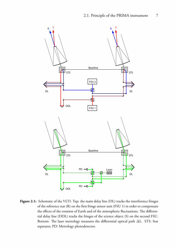
Figure 2.1 shows the layout of the VLT during interferometric operation. e light fromthe stellar object is collected using two telescopes and the white light interferometryfringes are observed on the fringe sensor unit (FSU). In order for fringes to be present,the optical path in both arms of the interferometer must be equal. is is achieved bymeans of moving delay lines between the telescopes and the fringe sensor unit.
e PRIMA instrument consists of two stellar interferometers, one for the reference starand one for the science object. e main delay line affects the path of both interferomet-ers in the same way. It is controlled by tracking the interference fringes of the referencestar and applies the corrections needed to compensate the effects of the rotation of Earthand of the atmospheric fluctuations on the optical paths. e differential delay line onlyaffects the optical path of the science interferometer and is controlled by tracking thefringes of the science object on a second FSU.
In astrometric mode, the PRIMA metrology measures the distance compensation ap-plied to the reference and science interferometers L1 and L2, respectively, by means of alaser interferometer in common path with the stellar light. As shown on Fig. 2.2, L1 andL2 depend on the distance between the telescopes, which is called the baseline (B), andthe angular position of the corresponding object. By measuring the differential com-pensation ∆L = L1 − L2, it is possible to calculate the angular separation between thereference and science objects.
2.1. Principle of the PRIMA instrument 7
STS STS
SR SR
FSU 1
FSU 2
DLDL
DDL
Baseline
STS STS
LaserPD
PD
DLDL
DDL
Baseline
Figure 2.1: Schematic of the VLTI. Top: the main delay line (DL) tracks the interference fringesof the reference star (R) on the first fringe sensor unit (FSU 1) in order to compensatethe effects of the rotation of Earth and of the atmospheric fluctuations. e differen-tial delay line (DDL) tracks the fringes of the science object (S) on the second FSU.Bottom: e laser metrology measures the differential optical path ∆L. STS: Starseparator, PD: Metrology photodetector.

8 Chapter 2. e Very Large Telescope Interferometer
S S
Baseline B
L1 = B sinα
α
Figure 2.2: Dependence of the distance compensation (L1) on the baseline (B) and the angularposition of the object (α).
2.2 Requirements for the laser metrology
e target accuracy for PRIMA in astrometric mode is of 10 µarcsec, or 5 × 10⁻¹¹ rad,with a baseline of 100m. is leads to a requirement on the accuracy of the measure-ment of ∆L of 5 nm, with a target resolution of less than 1 nm. is resolution mustbe reached with a minimum optical power of 20 nW. With a baseline of 200m, themaximum star separation of 1 arcmin leads to a maximum ∆L of 60mm. erefore, atarget range for the metrology system of 100mm was specified.
e maximum velocity of the main delay lines (DL) and of the differential delay line(DDL) at which the PRIMA metrology system should operate with the specified accur-acy is 10mm/s for the DL and 15mm/s for the DDL.emaximum velocity for whichthe system should be able to keep track of the interference fringes (slewing velocity) is36mm/s for the DL and 18mm/s for the DDL.
e rate of the data delivered by the metrology system should be selectable between0.5Hz and 8 kHz, with the value of ∆L averaged over the measurement period.
e laser source should have a wavelength above 1 µm to avoid stray light on the Siliconphotodetectors used for the adaptive optics of the VLT, but below 2 µm where astro-nomic observations are performed. e coherence length should be larger than 500m.erefore, a Nd:YAG laser at 1319 nm was chosen. In order to reach the target res-olution of 1 nm over a range of 100mm, the optical frequency of the laser should bestable to 10−8 and known with the same accuracy. e requirements are summarised inTable 2.1.

2.3. Concept of the PRIMA laser metrology 9
Differential OPD (∆L) Resolution < 1 nm
Accuracy < 5 nm
Max. range 100mm
Min. optical power 20 nW
Max. operating velocity DL 10mm/s
DDL 15mm/s
Max. slewing velocity DL 36mm/s
DDL 18mm/s
Output Data rate 0.5Hz − 8 kHz
Laser source Wavelength 1319 nm
Frequency stability 10−8
Table 2.1: Summary of the requirements for the PRIMA laser metrology.
2.3 Concept of the PRIMA laser metrology
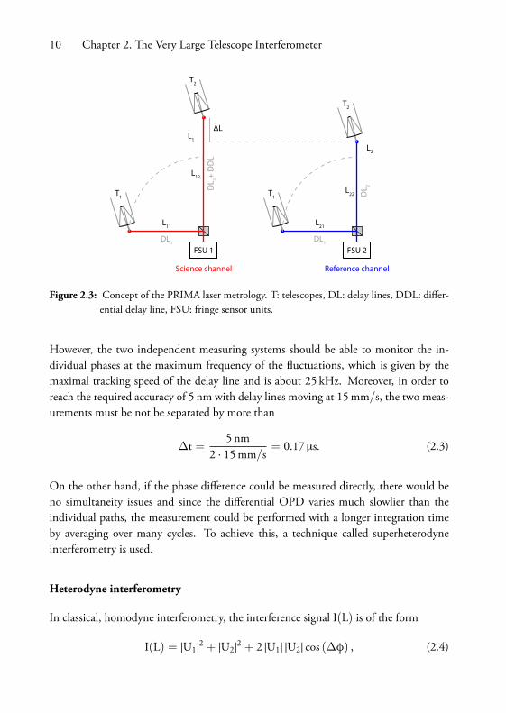
e value measured by the PRIMA metrology is ∆L = L1 − L2, the difference betweenthe optical path differences (OPD) of the reference and the science interferometers(Fig. 2.3). We call L11 and L12 the arm lengths of the science interferometer andL1 = L12 − L11 the OPD of the interferometer. Similarly, the arm lengths and theOPD of the reference interferometers are called L21, L22 and L2 = L22 − L21, respect-ively. Two laser interferometers are used to measure L1 and L2 from the interferometricphases φ1 and φ2 given by
φ1 =4πν1c
L1, φ2 =4πν2c
L2. (2.1)
A solution to measure ∆L is to measure φ1 and φ2 separately and compute the differ-ential OPD using the relation
∆L =c
4πν1φ1 −
c4πν2
φ2. (2.2)
10 Chapter 2. e Very Large Telescope Interferometer
FSU 1 FSU 2
Science channel Reference channel
DL1
DL 2+
DD
L
DL1
DL 2
L12
L11
L1
L22
L21
L2
∆L
T1
T2
T1
T2
Figure 2.3: Concept of the PRIMA laser metrology. T: telescopes, DL: delay lines, DDL: differ-ential delay line, FSU: fringe sensor units.
However, the two independent measuring systems should be able to monitor the in-dividual phases at the maximum frequency of the fluctuations, which is given by themaximal tracking speed of the delay line and is about 25 kHz. Moreover, in order toreach the required accuracy of 5 nm with delay lines moving at 15mm/s, the two meas-urements must be not be separated by more than
∆t =5 nm
2 · 15mm/s= 0.17 µs. (2.3)
On the other hand, if the phase difference could be measured directly, there would beno simultaneity issues and since the differential OPD varies much slowlier than theindividual paths, the measurement could be performed with a longer integration timeby averaging over many cycles. To achieve this, a technique called superheterodyneinterferometry is used.
Heterodyne interferometry
In classical, homodyne interferometry, the interference signal I(L) is of the form
I(L) = |U1|2 + |U2|
2 + 2 |U1| |U2| cos (∆φ) , (2.4)

2.3. Concept of the PRIMA laser metrology 11
with
∆φ =4πνc
L, (2.5)
where ∆φ is the phase difference of the interferometer, L the optical path difference andU1 and U2 are the amplitudes of the waves in each arm.
In heterodyne interferometry, however, a small shift f of the optical frequency of a fewtens of MHz is introduced between the two arms of the interferometer. e complexamplitudes of the two interfering waves are therefore given by
U1(z, t) = U01 eiφ1 ei2πνt,
U2(z, t) = U02 eiφ2 ei2π(ν+f)t,(2.6)
and the interference signal becomes
I(t) = |U01|2 + |U02|
2 + 2 |U01| |U02| cos (2πft + ∆φ)
= I1 + I2 + 2√I1I2 cos (2πft + ∆φ) .
(2.7)
Superheterodyne interferometry
In order to measure ∆L directly, without having to measure L1 and L2 separately andcompute the difference, a technique called superheterodyne interferometry is used [3].It consists of using two different heterodyne frequencies, f1 and f2, in the two interfer-ometers. Moreover, in order to avoid any crosstalk, an additional frequency offset f0is introduced between the two interferometers. erefore, the optical frequencies are νand ν + f1 for the science interferometer and ν + f0 and ν + f0 + f1 for the referenceinterferometer.
e interference signal for the two interferometers can be written as
I1(t) = I11 + I12 + 2√I11I12 cos(2πf1t + φ1),
I2(t) = I21 + I22 + 2√I21I22 cos(2πf2t + φ2),
(2.8)
where I11 and I12 are the intensities in each arm of the science interferometer, φ1 isthe phase difference of the science interferometer, and likewise I21, I22 and φ2 for thereference interferometer.
e phase difference of the science interferometer is linked to the OPD by
φ1 =4π(ν+ f1)
cL12 −
4πνc
L11 =4πνc
L1 +4πf1c
L12. (2.9)

12 Chapter 2. e Very Large Telescope Interferometer
Since only one delay line, L11, is moving the other one being passive, the term containingL12 will be constant. e phase therefore only varies with L1
φ1 =4πνc
L1. (2.10)
Similarly, the phase of the reference interferometer depends on L2 by
φ2 =4π(ν+ f0)
cL2. (2.11)
Superheterodyne detection consists of mixing both interference signals electronicallyafter detection. e signals are bandpass filtered around their heterodyne frequencies inorder to keep only the ac part, then they are mixed together and the result is bandpassfiltered around the difference between the two heterodyne frequencies. e result ofmixing the signals is their multiplication, which yields
I(t) ∝√I11I12 cos (2πf1t + φ1) ·
√I21I22 cos (2πf2t + φ2)
= I0[cos (2π (f1 + f2) t + φ1 + φ2)
+ cos (2π (f1 − f2) t + φ1 − φ2)].
(2.12)
Filtering around f1 − f2 gives
I(t) = I0 cos (2π (f1 − f2) t + φ1 − φ2) . (2.13)
In order to measure the phase φ1 − φ2 that leads to ∆L, a reference signal of the samefrequency with fixed phase must be generated. e superheterodyne detection processis depicted on Fig. 2.4. From Eqs. (2.10) and (2.11), we get for the phase difference
φ1 − φ2 =4πνc
L1 −4π(ν+ f0)
cL2
=4πνc
∆L −4πf0c
L2.(2.14)
We can see that due to the frequency offset f0 between the science and reference inter-ferometers, the measured phase not only depends on the differential OPD ∆L but alsoon the OPD of the reference interferometer L2. erefore, the variation of this OPDmust be monitored in order to be compensated. e phase shift δφ introduced by thevariation δL2 of the OPD is given by
δφ =4πf0cδL2. (2.15)

2.3. Concept of the PRIMA laser metrology 13
φ2
φ1
∆φ
I1( t ) ≈ cos(2πf
1t + φ
1)
I( t ) ≈ cos(2πf t + ∆φ)
I2( t ) ≈ cos(2πf
2t + φ
2)
f = f1 – f
2
∆φ = φ1 – φ
2
Heterodyne signals
Superheterodyne signalProbe
Probe
Reference
ReferenceProbe
Reference
Figure 2.4: Superheterodyne detection. e electronic mixing of the two heterodyne signals I1(t)and I2(t) results in the superheterodyne signal I(t), whose frequency and phase f and∆φ are equal to the difference of the frequencies and phases f1, f2 and φ1, φ2 of theheterodyne signals.
Since δφ depends only on the frequency difference f0, which is 78MHz in our case (seeTable 3.1), the required accuracy on δL2 in order to achieve 2π/1000 accuracy is notvery stringent:
∆(δL2) =c
4πf02π1000
= 1.9mm. (2.16)
A simple fringe counter on the reference interferometer can therefore be used to monitorδL2 within the target accuracy. If NFC is the current value of the fringe counter, δL2 isgiven by
δL2 =c
4π(ν+ f0)2πNFC ≈
c2ν
NFC, (2.17)
and
δφ =4πf0cδL2 =
2πf0ν
NFC. (2.18)
erefore, the differential OPD ∆L is given by
∆L =c
4πν(φ+ δφ) =
c4πν
(φ+
2πf0ν
NFC
). (2.19)

14 Chapter 2. e Very Large Telescope Interferometer
2.4 Summary of the requirements for the PRIMAmetrology
e PRIMAmetrology should measure ∆L with a resolution of 1 nm (2π/660 in phasefor λ = 1319 nm) and an accuracy of 5 nm (2π/130), with a maximum range of100mm. e minimum optical power is of 20 nW. e maximum velocities of thedelay lines and of the differential delay line under operating conditions are 10mm/sand 15mm/s, respectively. e maximum slewing velocities of the delay lines and ofthe differential delay line are 36mm/s and 18mm/s, respectively.
e output data rate should be selectable between 0.5Hz and 8 kHz and the internalsampling frequency (and thus the superheterodyne frequency) should be high enoughto allow the averaging of the value of ∆L over several cycles.
Furthermore, the frequency of the 1319 nm Nd:YAG laser should be stable to 10−8 andknown with the same accuracy.

Chapter 3
Digital phasemeter forsuperheterodyne detection
3.1 Superheterodyne detection
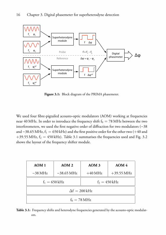
Figure 3.1 describes the principle of the superheterodyne phase measurement. eheterodyne signals at frequencies f1 and f2 are detected by four photodetectors andthe superheterodyne module performs the filtering and mixing operations described inchapter 2.3. It generates the superheterodyne signals at frequency f = f1 − f2 which arethen fed to the digital phasemeter that measures their phase difference ∆φ.
3.1.1 Frequency shifter module
e frequency shifter module generates the frequency shifts necessary to produce thedifferent heterodyne signals. e goal is to generate two heterodyne signals with a fre-quency difference ∆f = f1− f2 of a few hundreds of kilohertz in order to be fast enoughto allow an output averaged over several samples at the required 8 kHz, but slow enoughnot to introduce too stringent requirements on the analogue electronics. Moreover, thereshould be an offset f0 between the optical frequencies of the two interferometers, whichcan be sufficiently filtered to avoid crosstalk.
15
16 Chapter 3. Digital phasemeter for superheterodyne detection
Superheterodyne module
φ2
f2
∆φ
φ1
f1
Superheterodyne module
Digital phasemeter
φ2ref f
2
f ∆φref
f = f1 – f
2
∆φ = φ1 – φ
2
f ∆φ
φ1ref f
1
Probe
Reference
Figure 3.1: Block diagram of the PRIMA phasemeter.
We used four fibre-pigtailed acousto-optic modulators (AOM) working at frequenciesnear 40MHz. In order to introduce the frequency shift f0 = 78MHz between the twointerferometers, we used the first negative order of diffraction for two modulators (−38and−38.65MHz, f1 = 650 kHz) and the first positive order for the other two (+40 and+39.55MHz, f2 = 450 kHz). Table 3.1 summarises the frequencies used and Fig. 3.2shows the layout of the frequency shifter module.
AOM 1 AOM 2 AOM 3 AOM 4
−38MHz −38.65MHz +40MHz +39.55MHz
f1 = 650 kHz f2 = 450 kHz
∆f = 200 kHz
f0 = 78MHz
Table 3.1: Frequency shifts and heterodyne frequencies generated by the acousto-optic modulat-ors.

3.1. Superheterodyne detection 17
AOM
AOM
AOM
AOM
+38 MHz
+38.65 MHz
–40 MHz
Laser input
PM coupler
PM coupler
PM coupler650 kHz
450 kHz
–39.55 MHz
Figure 3.2: Layout of the frequency shifter module. AOM: acousto-optic modulators, PMcoupler: polarisation-maintaining fibre couplers.
3.1.2 Electronic signal processing
Figure 3.3 shows the schematic of the superheterodyne module, including the photode-tectors, the input bandpass filters, the mixer stage and the output bandpass filter with alimiting amplifier.
450 kHz
200 kHz
Science
650 kHz
Reference
Photodetectors
Bandpass filters
MixerBandpass filter
Limiter
Limiter
Limiter
Figure 3.3: Schematic of the superheterodyne module.

18 Chapter 3. Digital phasemeter for superheterodyne detection
–
+
VB
Vout
+
–
I = Popt
Sν
OPAhν
C
R
–+
Figure 3.4: Typical photodetector circuit. PD: photodiode, OPA: operational amplifier, R:transimpedance gain.
Photodetectors
Figure 3.4 shows a typical photodetector consisting of a photodiode and a transimped-ance circuit. e gain of the amplifier is given by the transimpedance resistor R. Fora given optical frequency ν, the sensitivity S of the photodetector is determined by thespectral sensitivity of the photodiode Sν and the transimpedance gain R as
S = R Sν = Rηehν
, (3.1)
where η is the quantum efficiency of the photodiode and e the electron charge. espectral sensitivity Sν relates the current I at the output of the photodiode to the opticalpower Popt, whereas the sensitivity of the photodetector S links the voltage Vout at theoutput of the amplifier to the optical power:
I = Popt Sν, (3.2)
Vout = RI = Popt S. (3.3)
e photodetectors of the phasemeter use InGaAs photodiodes with a spectral sensitivityof Sν = 0.88 A/W at 1.3 µm. e transimpedance gain is R = 1.4 × 10⁶ V/A, leadingto a sensitivity of S = 1.23V/µW.
Trigger error
In a zero-crossing phasemeter, the noise on the signal introduces an uncertainty on thetime of the crossing. Figure 3.5 illustrates this phenomenon. is uncertainty ∆t can

3.1. Superheterodyne detection 19
∆Vrms
∆t
Figure 3.5: Trigger error.
be calculated from the slope of the signal and the rms noise as
∆t =∆VrmsdVdt
∣∣∣V=0
. (3.4)
In the case of a cosine signal
V(t) = V cos (2πft + φ) , (3.5)
of amplitude V and frequency f, the slope is
dVdt
∣∣∣∣∣V=0
= 2πfV. (3.6)
Assuming that both the reference and the measurement signals contribute equally to thephase error δφ, we get
δφ = 2πf√
∆t2meas + ∆t2ref =√2
∆Vrms
V. (3.7)
e SNR, defined as the ratio of the electrical power of the signal and the electricalpower of the noise, is related to the rms noise by
SNR =Pel.signalPel.noise
=V2
⟨cos2 (2πft + φ)
⟩∆V2
rms=
12
V2
∆V2rms
. (3.8)

20 Chapter 3. Digital phasemeter for superheterodyne detection
erefore, the phase error can be expressed in terms of the SNR as
δφ =1√SNR
. (3.9)
To get the required phase resolution of 2π/660, the SNR of the electronic signals mustbe at least 11000 or, in logarithmic units, SNR > 40 dB.
Due to the movement of the delay lines at velocities up to 36mm/s, the frequency of theheterodyne signals is shifted by the Doppler effect during operation. In order to avoidintroducing a phase shift that depends on the movement of the delay lines, the phaseresponse of the photodetectors should be as flat as possible. In this intent, the bandwidthof the transimpedance amplifier was designed to be 7.5MHz, which is much higher thanthe frequency of the detected signals.
Bandpass filters
Tenth order Chebyshev bandpass filters are used to extract the heterodyne frequencies.However, the Doppler shift caused by the movement of the delay lines changes thefrequencies and if the phase responses of the 450 kHz and 650 kHz filters are different,a phase shift dependent on the velocity of the delay lines will be introduced. erefore,the phase response of the filters have to be matched to within 2π/660 (0.54 deg) overa width of 110 kHz, corresponding to the range of Doppler frequencies caused by themaximum speed of the delay lines of 36mm/s. It is not trivial to fulfil this requirementbecause the two bandpass filters operate around two different frequencies.
Limiting amplifiers and mixer
e 450 kHz and 650 kHz heterodyne signals are mixed and filtered around the su-perheterodyne frequency f = 200 kHz. e filters have a bandwidth of 55 kHz, cor-responding to the maximum Doppler shift caused by the movement of the differentialdelay line at a velocity of 18mm/s.
During the testing of the prototype version of the phasemeter, it was noticed that vari-ations of the amplitude of the heterodyne signals at the input of the mixer caused vari-ations of the phase of the superheterodyne signal. To solve this problem, limiting amp-lifiers were introduced at the mixer inputs to convert the sinusoidal heterodyne signalsinto square signals of constant amplitude. Other benefits of this configuration are thatthe mixing efficiency is higher compared to sinusoidal signals and that the amplitude

3.2. Digital phase measurement 21
of the square signals can be adjusted for maximum efficiency using an amplifier with avariable gain at the input of the mixer. Another limiting amplifier was placed after theoutput bandpass filter of the mixer to convert the superheterodyne signal into a squaresignal fed to the digital phasemeter.
e limiting amplifiers are composed of two stages. e first stage amplifies the signalwith a high gain and limits the amplitude using diodes and the second stage is a compar-ator that delivers a square signal in TTL format. e high gain of the amplifier results inan increased slope of the signal at zero-crossing, which renders the system less sensitiveto an offset of the comparator.
3.2 Digital phase measurement
e purpose of the digital phasemeter is to measure the phase between the 200 kHzreference and probe superheterodyne signals with a resolution of at least 2π/660. Itshould be able to monitor displacements of the differential delay line up to 120mm andshould perform averaging of data in order to measure with a frequency response between0.5Hz and 8 kHz.
Moreover, due to the frequency offset f0 between the science and reference channels, theOPD of the reference interferometer L2 has to be monitored using a fringe counter onthe 450 kHz heterodyne signal, as explained in chapter 2.3.
e digital logic of the phasemeter was implemented using programmable logic devices(PLD) of the MAX7000 family from Altera.
3.2.1 Phase-locked loop
A phase-locked loop (PLL) was used to generate the clock signals necessary to the oper-ation of the digital phasemeter. A 200MHz primary clock drives the fractional phase-meter and a 50MHz clock is used for the rest of the circuit, which can operate at lowerspeed.
Figure 3.6 shows the principle of the PLL. It is composed of a high-frequency voltage-controlled oscillator (VCO) at 200MHz and of a phase comparator circuit. e VCOfrequency is divided by 1024 to obtain a signal of roughly 200 kHz. e phase of thissignal is then compared to the phase of the reference superheterodyne signal. e low-pass filtered output of the phase comparator is fed back to the VCO. When the PLL

22 Chapter 3. Digital phasemeter for superheterodyne detection
Reference Reference 2
Clock
Clock 2
Reference Q
Reference PLL
Altera PLD
φ
Phase comparator
200 MHz VCO
Figure 3.6: Schematic of the phase-locked loop. Reference: reference superheterodyne signalat 200 kHz, Clock: 200MHz primary clock, Clock 2: 50MHz secondary clock,Reference 2: reference signal after clock synchronisation, ReferenceQ: reference signalin quadrature, Reference PLL: VCO frequency divided by 1024.
is locked, the frequency at the output of the VCO is 1024 times the frequency of thereference signal, or 200MHz.
We used aMini-Circuits POS-400P VCO and the phase comparator of an HEF4046BFPLL circuit. e frequency division was implemented with a digital counter in an AlteraPLD. Moreover, the same device was used to generate the secondary clock signal at50MHz as well as a reference signal in quadrature (phase shifted by π/2) used by thefractional phasemeter. Both the reference and the reference in quadrature were alsosynchronised with the primary clock to avoid stability problems in the digital phasemeterdue to asynchronous signals.
3.2.2 Digital zero-crossing phasemeter
Fractional phase
Figure 3.7 shows the principle of operation of a digital phasemeter. e goal is tomeasurethe phase between a reference and a probe signal of the same known frequency f . isis achieved by measuring the time between a raising edge of the reference signal and araising edge of the probe signal, using a digital counter. e counter is driven with aclock signal whose frequency fc gives the resolution δφ of the phasemeter. e phase φis calculated from the value of the counter Nφ and the resolution δφ. Nφ ranges from 0to N1, corresponding to phases between 0 and 2π. Since the frequency multiplier of thephase-locked loop must be a power of two and the resolution of the phasemeter mustbe at least 2π/660, the best value for N1 is 1024 and the counter has 10 bits.

3.2. Digital phase measurement 23
Count
Counter Enable
Signal
Reference
Clock
4 … 6
Figure 3.7: Principle of operation of a digital phasemeter. In this example the clock frequencyis 20 times higher than the signal frequency, therefore the resolution is 2π/20. Afterthe first measurement, the value of the counter is 4, corresponding to a phase of 2π/5or 72 deg.
e clock frequency fc is the frequency of the superheterodyne signal f multiplied by thePLL multiplier N1:
fc = N1 f. (3.10)
With a heterodyne signal at f = 200 kHz, the clock frequency of the digital phasemeteris thus 204.8MHz.
For the phase resolution δφ, which is given by the ratio of the signal and clock frequen-cies, we get then
δφ = 2πffc
=2πN1
=2π1024
, (3.11)
and the phase φ for a given measurement is calculated from the resolution and the valueof the counter Nφ by
φ = Nφ δφ = 2πNφN1
. (3.12)
In practice, problems can occur when the phase is near zero, because if the edges of thereference and probe signals are too close to each other, a new measurement could startbefore the previous one is read-out, resulting in an output value of zero. e solution isto use a second counter driven by a reference signal in quadrature to the other, i.e. phaseshifted by π/2. is way, for any phase, at least one of the two counters is read-outat the appropriate time and provides a valid phase value. When the value of the main

24 Chapter 3. Digital phasemeter for superheterodyne detection
counter is zero, the value of the quadrature counter is used instead, after being correctedto compensate for the phase shift introduced by the reference signal in quadrature.
Since the reference signal in quadrature is delayed by π/2, the correction that shouldbe added to the value of the counter is N1/4 = 256. Since N1 is a power of two, thisoperation can be easily achieved by acting only on the two most significant bits of Nφ.Equation (3.13) illustrate the logical operations used to perform this addition,
Fn−2
Fn−1 Fn−2 . . . F0+ 0 1 . . . 0
Fn−2 ⊕ Fn−1 Fn−2 . . . F0
(3.13)
where n = 10 is the maximum bit number of the counter and Fn−1 and Fn−2 are thetwo most significant bits of the fractional phase measured by the quadrature counter.
Integer phase
In addition to the fractional phasemeter, an integer fringe counter is needed in order tokeep track of the distance covered by the delay lines. An up/down counter is triggeredevery time the fractional phase crosses zero, with the direction of the count matchingthe direction of the crossing.
Figure 3.8 shows the control signals used to enable the counter and to choose the direc-tion. e range of values of the fractional phase is split into four quadrants. e counteris triggered by the clock signal CCk every time the phase changes quadrants. If the previ-ous and current values of Cnt are 1, it means that the value crossed zero and the counteris enabled. e counting direction is given by the UD signal. Equations (3.14)–(3.16)show how the control signals are generated from the two MSBs of the fractional phase
Cnt = Fprevn−2 ⊕ Fn−2, (3.14)
UD = Fn−1 ⊕ Fn−2, (3.15)
CCk = UDprev ⊕UD. (3.16)
Figure 3.9 shows the logic diagram of the fractional phasemeter. Counter A is enabled onan edge of the reference signal, whereas counter B is enabled on an edge of the referencesignal in quadrature. On the next edge of the probe signal, both counters are disabled,their values are loaded in a buffer and the counters are reset. e value of the quadrature

3.2. Digital phase measurement 25
Count
Up/Down
Cou
nt
Up
/Dow
n
Clock
enable enable
up
down
t
2π
π
φ
Figure 3.8: Control signals for the integer fringe counter. Cnt: count enable, UD: up/down,CCk: counter clock.
Signal
Reference
Clock
Reference Q
Fractionalphase
CounterBen
clr
CounterAen
clr
D = 0
DN
1
4+
0
1
reset
set
reset
set
DDD
Figure 3.9: Principle of the instantaneous phasemeter, fractional part. Reference: referencesignal, Reference Q: reference signal in quadrature, Signal: probe signal, Clock:200MHz clock, Counter A: main counter, Counter B: quadrature counter.

26 Chapter 3. Digital phasemeter for superheterodyne detection
en
up/down
Counter
Cnt
UD
CCk
Fn–1
Fn–2
IntegerphaseD
Figure 3.10: Principle of the instantaneous phasemeter, integer part. Fn−1, Fn−2: two MSBs ofthe fractional phase, Counter: integer fringe counter, UD: count direction up/down,CCk: counter clock, Cnt: counter enable.
counter is then compensated by adding N1/4 to it. If the value of counter A is zero, itmight mean that the value was read before it was ready. erefore, the value of counter Bis used instead by routing it to the output of the phasemeter by means of a multiplexer.
Figure 3.10 shows the logic diagram of the integer fringe counter. e two most signi-ficant bits of the fractional phase, Fn−1 and Fn−2, are used to generate the control signalsdescribed earlier: counter enable, clock and direction. e maximum distance to bemonitored by the phasemeter is 120mm (mechanical). With a wavelength of 1319 nm,18 bits are sufficient to store values up to 173mm (218 × λ/2). For safety, an extra bitwas allocated to the integer fringe counter. e output of the digital phasemeter is com-posed of the integer phase on 19 bits and the fractional phase on 10 bits, resulting in a29 bit word. e least significant bit (LSB) of this value represents a phase of 2π/1024,corresponding to a distance of 0.64 nm (mechanical).
Maximum speed of the differential delay line
In order that the integer fringe counting works correctly, the fractional phase must notchange by more than π/2 between two measurements. Otherwise, the phase skips aquadrant and the zero crossing is not detected properly. is condition limits the speedfor the differential delay line to
vmax =λ/4T
= 66mm/s, (3.17)
where the wavelength is λ = 1.3 µm and the time between the measurements is T =5 µs, corresponding to the period of the 200 kHz.

3.2. Digital phase measurement 27
3.2.3 Averaging of phase data
e resolution of the phasemeter can be improved by averaging its output over multiplemeasurements. For ideal signals, the phase resolution is given by the frequency of theclock signal
δφideal = 2πffc
=2πN1
. (3.18)
Introducing the error due to the noise in the signal leads to a phase resolution for a singlemeasurement of
δφsingle =
√4π2
N21
+1
SNR. (3.19)
In the case of a phasemeter averaging data on N = Tf independent measurements, theerror introduced by the limited SNR is reduced by a factor of
√Tf . e error due to
the clock frequency, however, is a rounding error which is always the same for a givenphase. It is therefore not reduced by averaging
δφavg =
√4π2
N21
+1
Tf SNR. (3.20)
Another benefit of on-board averaging is that it reduces the data rate at the output ofthe phasemeter by a factor N and therefore reduces the load on the local control unit(LCU) to acquire and process data.
In order to average data over several measurements, the phasemeter must sum and dividethem by the number of samples. However, division by an arbitrary number is not easilyimplemented in the programmable logic used to build the phasemeter. For this reason,the phasemeter prototype only supported averaging on a number of samples that wasa power of two, because the division then reduced to shifting the bits of the summedphase by log2 N positions.
For the final version of the phasemeter, averaging over an arbitrary number of sampleswas required. Using a digital signal processing board was considered but it added toomuch complexity to the system. erefore, the averaging operation has been split betweenthe phasemeter and the LCU in charge of reading the phasemeter output. e phase-meter adds the instantaneous phase values and counts the number of samples and theLCU performs the division.

28 Chapter 3. Digital phasemeter for superheterodyne detection
Cnt
DD
D
D
D
D
Phase
Sum
Ready
Trigger
Count
Σ
Figure 3.11: Principle of the phase adder. Σ: adder, Cnt: sample counter, D: flip-flops, Phase:integer and fractional phase, Ready: a new phase value is ready, Trigger: end of thecurrent averaging period and start of the next one.
Figure 3.11 shows the principle of the phase adder. When a new phase measurementbecomes available, a Ready signal is received from the instantaneous phasemeter. eadder adds the new values for the integer and fractional phase to the previous value ofthe sum and the sample counter is incremented. When a trigger signal is received at theend of the averaging period, the output latches are loaded with the current values of thesummed phase and the sample counter and the adder latch are reset.
e integration time for the averaged phase ranges from 125 µs (8 kHz) to 2 s (0.5Hz),corresponding to a number of samples between 25 and 400000. e width of the samplecountermust therefore be at least 19 bits (log2 400000 = 18.6) and the width of the adder48 bits (29 + 19).
3.2.4 Error compensation fringe counter
Figure 3.12 shows the principle of the error compensation fringe counter. It consists oftwo digital counters, one for the signal and one for the reference, and a subtractor thatcomputes the difference NFC between the value of the two counters. e variation δL2of the OPD of the reference interferometer is then calculated from Eq. (2.17)
δL2 =c2ν
NFC. (3.21)

3.2. Digital phase measurement 29
Signal
Reference
NFC
SignalCounter
ReferenceCounter
D D D
∆
Figure 3.12: Error compensation fringe counter. D: flip-flops, ∆: subtractor.
3.2.5 Status registers
In addition to the summed phase value, the number of samples and the error compens-ation fringe counter value, some status information was added to the data provided bythe phasemeter. is information includes:
• e dc level of each photodetector (4 × 8 bits);
• Whether the heterodyne signals are present (4 bits);
• Whether the reference and probe superheterodyne signals are present (2 bits);
• Whether there was an overflow of the instantaneous phasemeter or of the errorcompensation fringe counter (2 bits);
• Whether a trigger or a reset signal was detected (2 bits).
For the dc level of the photodetectors, four Maxim MAX152 8-bit analogue to digitalconverters were used. For the detection of the heterodyne signals, a frequency counterwas implemented in four Microchip PIC12 8-bit microcontrollers. e heterodyne sig-nal is considered present if its frequency is comprised within the 110 kHz bandwidthspecified for the input bandpass filters.

30 Chapter 3. Digital phasemeter for superheterodyne detection
MSB
Word
5
6
4
1
3
2
LSB
SOT (4 bits) 0
0
0
0
DC Ref 450k (8 bits)DC Probe 450k (8 bits) DC Ref 650k (8 bits)DC Probe 650k (8 bits)
Packet (4 bits)
Packet (4 bits)
EOT (4 bits)
Phase sum, high (16 bits)
Phase sum, low (32 bits)
Number of samples (19 bits)
Error compensation (24 bits)
Status (10 bits)
Figure 3.13: Data transfer packet.
3.2.6 Data transfer
e interface between the phasemeter and the LCU is a 32-bit digital I/O board. edata from the phasemeter must therefore be transmitted in a packet of several words.Figure 3.13 shows how the data was distributed over a packet of six 32-bit words.
In order to make sure that all packets were acquired by the LCU and that the acquisitionis synchronised with the phasemeter, two control bytes, named Start of Block (SOB) andEnd of Block (EOB) respectively, were added to the beginning of the first and the endof the last words of the packet. e first four bits contain the packet number, rangingfrom 0 to 15 and incremented for each packet transferred. e last four bits have fixedvalues.
Data integrity is checked by ensuring that:
• e packet number is the same for SOB and EOB;
• e last four bits of SOB and EOB have the correct values;
• e packet number is the number of the previous packet plus one.

Chapter 4
Frequency stabilisation of aNd:YAG laser
4.1 Frequency noise of the laser
e frequency noise of the laser wasmeasured using two different techniques. Long-termfrequency fluctuations were measured by monitoring the beat frequency between twofree-running lasers of the same model and the noise at higher frequencies was measuredby means of an interferometer with a very large optical path difference, using a 1 kmfibre delay.
4.1.1 Measurement of the beat frequency
Figure 4.1 shows the set-up used to monitor the beat frequency between the two free-running lasers. e laser beams were combined using a fibre coupler. e beat frequencywas detected with a high-speed photodetector (Newport) andmeasured with a frequencycounter (HP53131). e integration time was 100ms and the sampling rate 1Hz.
e power spectral density (PSD) of the the frequency noise of an individual laser wasdeduced from these measurements by dividing by two the PSD in Hz2/Hz of the beatfrequency measurement. Figure 4.2 shows the measurement of the beat frequency overone hour and the deduced PSD for a single laser.
31

32 Chapter 4. Frequency stabilisation of a Nd:YAG laser
Nd:YAG 1
Nd:YAG 2
PhotodetectorFibre coupler
Figure 4.1: Set-up for the measurement of the beat frequency between two free-running lasers.
Figure 4.2: Beat frequency measurement for the free-running lasers (left) and deduced frequencynoise PSD for a single laser (right). One can see that the frequency noise exhibits abehaviour close to 1/f noise.
4.1.2 Measurements at large OPD
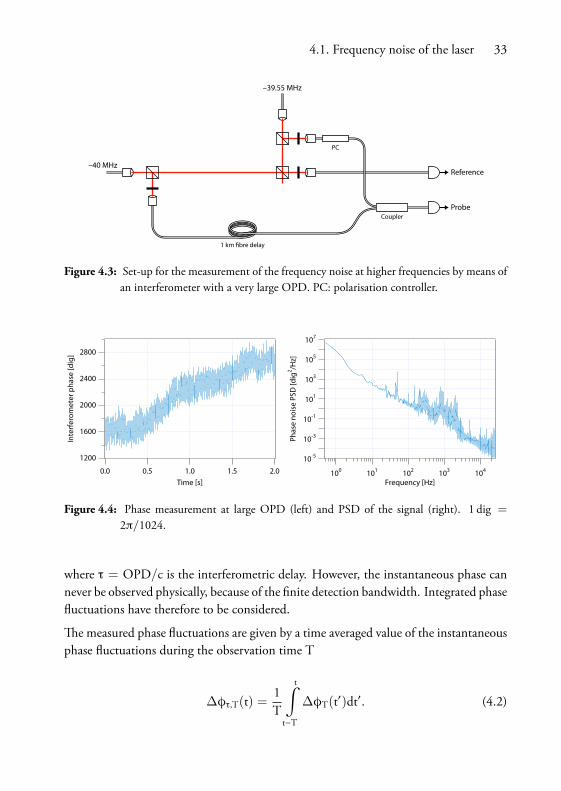
Figure 4.3 shows the set-up used to measure the frequency noise of the laser at higherfrequencies using the PRIMA phasemeter (see chapter 3, Fig. 3.1). e main interfer-ometer had a large OPD made with a length of fibre of 1 km. A second interferometerwas used for the reference signal. In order to monitor the individual OPD of the in-terferometer, the 450 kHz signal was monitored at 50 kHz over 2 s using the PRIMAphasemeter. An electrically generated signal common to the reference and probe wasused for the 650 kHz channel.
Figure 4.4 shows the phase measurement and the PSD of the phase fluctuations. It canbe shown [4] that the relation between the PSD of the instantaneous phase fluctuationsS∆φτ(f) and the PSD of the laser frequency fluctuations Sδν(f) is
S∆φτ(f) = 4π2τ2Sδν(f)(sinπ f τπ f τ
)2, (4.1)
4.1. Frequency noise of the laser 33
–40 MHz
–39.55 MHz
PC
Coupler
1 km fibre delay
Reference
Probe
Figure 4.3: Set-up for the measurement of the frequency noise at higher frequencies by means ofan interferometer with a very large OPD. PC: polarisation controller.
Figure 4.4: Phase measurement at large OPD (left) and PSD of the signal (right). 1 dig =
2π/1024.
where τ = OPD/c is the interferometric delay. However, the instantaneous phase cannever be observed physically, because of the finite detection bandwidth. Integrated phasefluctuations have therefore to be considered.
e measured phase fluctuations are given by a time averaged value of the instantaneousphase fluctuations during the observation time T
∆φτ,T(t) =1T
t∫t−T
∆φT(t′)dt′. (4.2)

34 Chapter 4. Frequency stabilisation of a Nd:YAG laser
is averaging introduces a factor(sinπ f Tπ f T
)2which, if the interferometric delay is much
smaller than the integration time, dominates over(sinπ f τπ f τ
)2. us, the PSD of the phase
fluctuations becomes
S∆φτ,T(f) = 4π2τ2Sδν(f)(sinπ f TπfT
)2. (4.3)
Assuming that the phase noise measured in Fig. 4.4 is mainly caused by the laser fre-quency noise spectrum, we can deduce from Eq. (4.3) the power spectral density of thelaser frequency fluctuations. For these measurements, the integration time T was of20 µs and the interferometric delay τ is given by OPD/c, where OPD = 1.5 km for a1 km fibre delay, since the index of refraction of the fibre is about 1.5.
Figure 4.5 shows the frequency noise spectrum of the laser estimated from the beatfrequency and the large OPD measurements. A white noise level was assumed above10 kHz, but the 1/f part may still be present until higher frequencies.
Figure 4.5: Estimated frequency noise spectrum of the laser.

4.1. Frequency noise of the laser 35
4.1.3 Required frequency noise spectrum
e variance of the measured phase fluctuations⟨∆φ2
τ,T
⟩is obtained by using the Par-
seval relation, which gives
⟨∆φ2
τ,T
⟩=
∞∫0
S∆φτ,T(f)df. (4.4)
Assuming as an approximation a white frequency noise within the detection bandwidthfor the stabilized laser, i.e. Sδν(f) = C0, for f < B = 1/2T, we have⟨
∆φ2τ,T
⟩≈ 2π2C0
τ2
T= 4π2C0τ
2B. (4.5)
To achieve the desired accuracy of 5 nm the maximal phase variations must be less than2π/132. erefore, the standard deviation σφ must be less than 2π/400 (three sigma).Using Eq. (4.5), we see that the value for C0 must fulfil the condition
C0 <σ2φ
4π2τ2B. (4.6)
For τ = 120mm/c = 0.4 ns and B = 8 kHz, we see that C0 < 5 × 10⁹ Hz2/Hz. epower spectral density of the remaining frequency fluctuations must therefore be less
Figure 4.6: Required frequency noise spectrum for the stabilised laser.

36 Chapter 4. Frequency stabilisation of a Nd:YAG laser
than 5 × 10⁹ Hz2/Hz (or 7.1 × 10⁴ Hz/Hz0.5) for frequencies f < 8 kHz. e powerspectral density shown in Fig. 4.6 allows therefore to fulfil this requirement. As it canbe seen, the cut-off frequency of the regulator does not need to be higher than 1Hz.
4.2 Absolute stabilisation
4.2.1 Absolute frequency references
e tunable range on the 1.3 µmNd:YAG laser is 50GHz, corresponding to wavelengthsbetween 1319 and 1319.3 nm. Table 4.1 shows a list of atomic or molecular frequencyreferences with absorption lines close to this range that may be suitable for absolutefrequency stabilisation [5].
However, none of these materials are very convenient, either requiring a very long ab-sorption path (up to 10m to reach a few tens of per cent absorption) or being dangerousand causing handling difficulties.
Gas Wavelength [nm] Comments
Carbon Dioxide 1311.8–1320 Very weak lines.
Water vapour 1280–1320 Very weak lines.
Hydrogen Fluoride 1278–1321.2 Highly corrosive.
Hydrogen Sulphide 1280–1320 Toxic.
Nitrate 1315–1320 Complex spectrum, maybe noabsorption line within the laserrange.
Methane 1312–1320 No absorption line within thelaser range.
Table 4.1: Atomic or molecular frequency references with absorption lines within 1319–1319.3 nm.

4.2. Absolute stabilisation 37
Second-harmonic Fundamental Transition
659.588 nm 1319.176 nm P(49)6-6
659.570 nm 1319.140 nm R(55)6-6
659.549 nm 1319.098 nm P(48)6-6
659.531 nm 1319.062 nm R(54)6-6
659.529 nm 1319.059 nm P(111)5-5
Table 4.2: Iodine absorption lines within the tuning range of the Nd:YAG laser.
4.2.2 Stabilisation of the second-harmonic wavelength on iodine
Another technique, first reported by Arie et al. [6], is to generate the second-harmonicof the Nd:YAG laser (at 659.5 nm) and stabilise it on iodine. Iodine is a good candidatefor laser stabilisation as its absorption lines are well known and not much subject totemperature drifts (about 10 kHz/°C).
ere are ten absorption lines in iodine within the tuning range of the laser. e fivestrongest ones are shown in Table 4.2. e transition used by Arie et al. was P(48)6-6.An iodine cell of length 13 cm was heated to 57 °C, leading to an absorption of about25% for a Doppler-broadened width of 800MHz. is is the technique that has beenretained for the stabilisation of the laser for the PRIMA metrology.
4.2.3 Centre-of-fringe locking
e stabilisation principle called centre-of-fringe locking [7, 8] consists of using the firstderivative of the transmission of the frequency reference as the frequency discriminant.
Figure 4.7 shows the transmission of an absorption line, as well as its first derivative.e absorption line is described in a good approximation by a Lorentzian line shape
T(ν) = 1 − Amax(∆ν/2)2
(ν − ν0)2 + (∆ν/2)2, (4.7)
where Amax is the absorption coefficient of the line, ∆ν the linewidth (FWHM) and ν0the centre frequency. One can see that the derivative is zero at the centre frequency ν0

38 Chapter 4. Frequency stabilisation of a Nd:YAG laser
Figure 4.7: An absorption line approximated by a Lorentzian shape and its first derivative.
and changes sign with (ν−ν0), making it a convenient error signal for the feedback loopof the frequency stabilisation.
It is possible to obtain an error signal proportional to the derivative of the absorptionline by modulating the frequency of the laser light
ν`(t) = ν+ νFM sin(2πft), (4.8)
where ν` is the frequency of the modulated laser light, νFM the frequency excursion andf the modulation frequency. Assuming a monochromatic wave, the transmitted light isgiven by
Pout(ν`) = PinT(ν`), (4.9)
where Pin is the power of the incident beam. By approximating T(ν`) with a first-orderTaylor series around the average frequency ν, the transmitted power becomes
Pout(t) = Pin [T(ν) + T′(ν)νFM sin(2πft)] , (4.10)
where T′(ν) is the first derivative of the transmission curve. e sinusoidal function atfrequency f is thus proportional to the first derivative of the transmission function.
e stabilisation principle is shown in Fig. 4.8. Synchronous detection is used tomeasurethe component at frequency f of the transmitted power, resulting in the error signal pro-

4.2. Absolute stabilisation 39
PZT
Temp
25%
75%
Dichroic filter
Detector EOM Iodine cell SHG
To PRIMA Metrology
EOM driver 25 MHz
Digital PI regulator
Lock-in amplifier
Laser
Figure 4.8: Stabilisation principle. SHG: second harmonic generation crystal, EOM: electro-optic modulator.
portional to T′(ν). e frequency modulation is achieved using an external frequencyor phase modulator. From Eq. (4.7), we can show that the slope of the frequency dis-criminant is
SFM = T′′(ν0) νFM =8Amax
∆ν2νFM, (4.11)
assuming a frequency excursion smaller than the linewidth. We note that this techniqueis insensitive to the laser power fluctuations and to the change of the absorption coef-ficient of the cell. In addition, synchronous detection allows to work at relatively highfrequencies (f > 10 kHz), where the 1/f noise of electronic components is no longerdominant.
Required optical power in the second harmonic
Assuming an input power Pin of 300 nW, which is a reasonable minimum for whatcan be expected after second harmonic generation, an absorption coefficient Amax of25% and a linewidth ∆ν of 800MHz, one can calculate the minimum detectable fre-quency drift δν, using a commercially available photodetector (Analog Modules, modelno 712A-2) with a voltage sensitivity SVP of 0.7 V/µW and a noise-equivalent power(NEP) of 2.1 pW/
√Hz. e voltage sensitivity at the output of the photodetector will
be
SVF = Pin SFM SVP = Pin8Amax
∆ν2νFM SVP = 0.052V/GHz. (4.12)
e detection bandwidth does not need to be very high, since the cut-off frequency ofthe regulator does not need to be higher than 1 Hz. erefore a cut-off frequency of 100

40 Chapter 4. Frequency stabilisation of a Nd:YAG laser
Hz for the lock-in amplifier is high enough. For a bandwidth B of 100 Hz, the voltagenoise is
σν = NEP SVP√B = 0.015mV. (4.13)
e signal-to-noise ratio of the detected signal for a frequency drift δν is
SNRac =(SVF δν)
2 ⟨cos2(2πft)
⟩σ2ν
=12
(SVF δν)2
σ2ν. (4.14)
e minimal detectable frequency drift δνmin is the value for which SNRac = 1. Wefind a value of δνmin = 400 kHz, which is well below the required 2MHz frequencystability. Synchronous detection should therefore allow to get the desired stability evenfor a second-harmonic power as low as 300 nW and a detection bandwidth of B =100Hz.
4.3 Second-harmonic generation
Second-harmonic generation uses the nonlinear dielectric properties of certain classesof crystals to generate a wave whose frequency is the double of that of the incomingwave [9, 10, 11]. e optical electric field E produces a polarisation P with a linear anda quadratic response
Pi = ε0χ(1)ik Ek + ε0χ
(2)iknEkEn i = x, y, z. (4.15)
where χ(1)ik and χ(2)ikn are respectively the linear and second-order nonlinear optical sus-ceptibilities of the crystal. Summations over repeated indices are assumed.
is nonlinear response allows an exchange of energy between electromagnetic fields ofdifferent frequencies. In the case of second-harmonic generation, this effect is used totransfer part of the energy of a wave of frequency ω to its second-harmonic at 2ω.
4.3.1 Birefringent phase matching
e general case for describing second-harmonic generation is three-wave mixing. eincoming beam is represented by twowaves of wave vectors k1 and k2 and of frequencyω

4.3. Second-harmonic generation 41
and the outgoing beam by a wave of wave vector k3 and of frequency 2ω. e phasematching condition must be fulfilled in order for second-harmonic light to be generated
k3 = k1 + k2. (4.16)
If the three waves propagate in the same direction, it becomes
2n3(2ω) = n1(ω) + n2(ω). (4.17)
Since the nonlinear medium is dispersive, this condition is in general not fulfilled. How-ever, by taking advantage of the birefringence of the crystal, phase matching can often beachieved by choosing an appropriate polarisation and direction of the incoming beamrelative to the crystal axes. is is called birefringent phase matching. Two types of phasematching are generally employed. ey are described here for a uniaxial crystal with anordinary index of refraction no and an extraordinary index ne.
In type I phase matching, the fundamental and harmonic are orthogonally polarised.e input is an extraordinary beam for which the index of refraction is n1 = n2 =nωe (θ), where θ is the angle between the axes of the crystal and the direction of propaga-tion. e output is an ordinary beam for which the index of refraction is n3 = n2ωo . ephase matching condition is
1(n2ωo )2
=1
(nωe (θ))2=
cos2 θ(nωo )2
+sin2 θ(nωe )2
. (4.18)
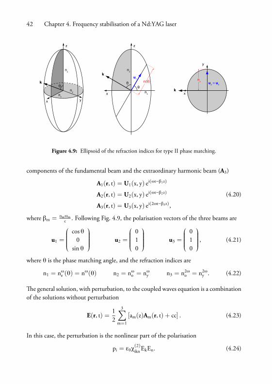
In type II phase matching, the incoming wave is polarised at 45 degrees relative to theaxes of the crystal (Fig. 4.9). e input is therefore the combination of an ordinary andan extraordinary beam, for which the index of refraction is n1 = nωe (θ) and n2 = nωo ,respectively. e output can be either an ordinary or an extraordinary beam. In the caseof an ordinary beam, the refractive index is n3 = n2ωo . e phase matching condition is
2n2ωo = nωe (θ) + nωo . (4.19)
4.3.2 Conversion efficiency
e first approach considered was to use type II phase matching in a KTP crystal togenerate the second harmonic light needed for the laser stabilisation.
e expected conversion efficiency in KTP can be calculated using coupled waves the-ory. e solutions without perturbation are the ordinary (A1) and extraordinary (A2)
42 Chapter 4. Frequency stabilisation of a Nd:YAG laser
y
u2 = u
3
x k
ny
x
z
θ θ
nx
nz
u1
k
n(θ) θ
z
x
k
nx
ny
nz
y
Figure 4.9: Ellipsoid of the refraction indices for type II phase matching.
components of the fundamental beam and the extraordinary harmonic beam (A3)
A1(r, t) = U1(x, y) ei(ωt−β1z)
A2(r, t) = U2(x, y) ei(ωt−β2z)
A3(r, t) = U3(x, y) ei(2ωt−β3z),
(4.20)
where βm = nmωmc . Following Fig. 4.9, the polarisation vectors of the three beams are
u1 =
cos θ0
sin θ
u2 =
010
u3 =
010
, (4.21)
where θ is the phase matching angle, and the refraction indices are
n1 = nωe (θ) = nω(θ) n2 = nωo = nωy n3 = n2ωo = n2ωy . (4.22)
e general solution, with perturbation, to the coupled waves equation is a combinationof the solutions without perturbation
E(r, t) =12
3∑m=1
[am(z)Am(r, t) + cc] . (4.23)
In this case, the perturbation is the nonlinear part of the polarisation
pi = ε0χ(2)iknEkEn. (4.24)

4.3. Second-harmonic generation 43
e coupled waves equation for the second harmonic is
da3dz
=iµ0
2TW3β3eiβ3z
∫dxdy
∫T
dtU∗3(x, y)e−iω3t · p(r, t). (4.25)
In this particular case, the propagation direction and the polarisations have been chosenfor the phase matching condition to be fulfilled. In addition, the following assumptionsare made:
• 1Wm
∫dxdyU∗m(x, y) = um;
• u3 has only a y component;
• e phase matching condition only preserves terms in a1a2, containing χ(2)yyx and
χ(2)yyz ;
• In KTP, χ(2)yyx is (nearly) zero.
Equation (4.25) for the second harmonic then becomes
da3dz
= −2iωn3cχ(2)yyz a1a2 sin θ. (4.26)
In order to calculate the conversion efficiency, intensities must be introduced by
Im =12
(ε0
µ0
) 12
nm |am|2 . (4.27)
I1 and I2 are half of the intensity If of the fundamental beam each and I3 is the intensityof the second harmonic
I1 = I2 =12If I3 = Ih. (4.28)
Moreover, since the conversion efficiency is very small, the amplitude of the fundamentalcan be assumed to be constant over the length of the crystal, leading to
a1(z) = a10 a2(z) = a20. (4.29)
erefore
a3(z) = −2iωn3cχ(2)yyz a10a20 sin θ z, (4.30)

44 Chapter 4. Frequency stabilisation of a Nd:YAG laser
and the conversion efficiency η is calculated as
η =I3
I1 + I2
=n3
∣∣∣a3(`)∣∣∣2n1 |a10|2 + n2 |a20|2
= 2(µ0
ε0
) 32 ω2`2
n3(ε0χ
(2)yyz sin θ
)2If ,
(4.31)
where ` is the length of the crystal and n3 = n1n2n3.
e indices of refraction of KTP were calculated using the Sellmeier equation [12]
n2i (λ) = ai + βi ∆T2 +bi + δi ∆T2
λ2 − ci + φi ∆T2 − [di + ρi ∆T2]λ2. (4.32)
At room temperature, the temperature-dependant coefficients can be left out of the equa-tion
n2i (λ) = ai +biλ2 − ci
− di λ2. (4.33)
Using the coefficients from Table 4.3, the indices of refraction of KTP at 1319 nm and659.5 nm were calculated as
nωx = 1.7339 nωy = 1.74164 nωz = 1.82153
n2ωx = 1.76072 n2ωy = 1.77026 n2ωz = 1.85919.
Coefficient x y z
ai 3.0065 3.0333 3.3134
bi 0.03901 0.04154 0.05694
ci 0.04251 0.04547 0.05657
di 0.01327 0.01408 0.01682
Table 4.3: Sellmeier equation parameters for KTP.
4.3. Second-harmonic generation 45
One can see that there is a small difference of index between the x and y directions, andtherefore KTP is not really a uniaxial crystal. However, it was treated as uniaxial forsimplification, the much higher index n3 playing the role of the extraordinary index ne.
e phase matching condition β1 + β2 − β3 = 0 gives
nω(θ) + nωy − 2n2ωy = 0. (4.34)
With nω(θ), the equation of the ellipsoid of refraction indices for the extraordinarybeam, can be solved for θ(
nω(θ) cos θnx
)2+
(nω(θ) sin θ
nz
)2= 1. (4.35)
It gives the phase matching angle θ = 60.4°.
e nonlinear electric susceptibility for KTP can be found in [13]
d31 = 6.5pmV
= χ311 = χ113 = χ131
d32 = 5.0pmV
= χ322 = χ223 = χ232
d33 = 13.7pmV
= χ333
d34 = 7.6pmV
= χ332 = χ323 = χ233
d35 = 6.1pmV
= χ331 = χ313= χ133.
(4.36)
For a crystal of a length of 8mm, with the beam focussed to a diameter 2w0 of 60 µm, asrecommended in [10] so that the Rayleigh distance z0 is equal to half the length of thecrystal, the calculated conversion efficiency η was of 3.1 × 10⁻⁵, leading to an expectedoutput power of 1.55 µW for an input power of 50mW.
However, the experimental results did not match this estimation. With an input powerof 60mW, only 17 nW of second harmonic light were obtained, corresponding to an ef-ficiency of 3×10⁻⁷. e cause of this reduced efficiency was identified to be birefringentwalk-off.
4.3.3 Birefringent walk-off
In anisotropic materials, the electric field E is not parallel to the electric induction D(Fig. 4.10). As a result, the wave vector k (perpendicular to D) is not parallel to the

46 Chapter 4. Frequency stabilisation of a Nd:YAG laser
α αθ
D E z
x
k
S
Figure 4.10: Birefringent walk-off.
Poynting vector S (perpendicular to E). is is know as birefringent walk-off. In the caseof second harmonic generation with Type II phase matching, the two components ofthe fundamental beam separate spatially because of this, and the interaction length (andtherefore the conversion efficiency, which is proportional to the square of the interactionlength) is reduced.
e relation between D and E is given by
Di = ε0εikEk, (4.37)
ε is related to the refractive indexes of the material by
ε =
n2x 0 00 n2y 00 0 n2z
. (4.38)
us we have
D =
Dcos θ
0D sin θ
E =Dε0
cos θ/n2x
0sin θ/n2z
. (4.39)
e walk-off angle α can then be calculated using the relation
cosα =D · E|D||E|
=
(cos θnx
)2+
(sin θnz
)2√cos2 θn4x
+ sin2 θn4z
. (4.40)
In KTP, in the conditions described above, the walk-off angle is of 43mrad, whichgives an interaction length of about 1.5mm for a beam diameter of 2w0 = 60 µm.

4.3. Second-harmonic generation 47
Collimating lens
SHG crystalPBS
PBS
Figure 4.11: Set-up for walk-off compensation.
e efficiency is therefore reduced to 10−6, which is closer to the 3 × 10⁻⁷ obtained inlaboratory.
A set-up for walk-off compensation was proposed and is depicted on Fig. 4.11. e ver-tical and horizontal components of the input polarisation are separated using a polarisingbeam splitter. A shift in the x-direction is introduced and the beams are recombined.Because of the focussing lens, the shift will introduce an angle between the two polar-isations that can be used to compensate the walk-off angle.
4.3.4 Quasi-phase matching in periodically-poled crystals
Given the relatively complex set-up required to compensate the walk-off angle and theapparition of periodically-poled nonlinear crystals for quasi-phase matching, the bi-refringent phase matching approach was abandoned in favour of quasi-phase matching.
Quasi-phase matching takes advantage of the fact that when the phase matching condi-tion is not fulfilled, as long as the phase between the input and the output is less than180 deg, energy flows from the fundamental to the harmonic frequency. is flow is re-versed for phases greater than 180 deg. e coherence length of the crystal is the distancefor which the phase is less than 180 deg.
In periodic poling, the axes of the crystal are flipped after each coherence length, whichresults in a phase change and the energy continues to flow from the fundamental tothe harmonic (Fig. 4.12). Periodic poling is achieved by periodic ferroelectric domain

48 Chapter 4. Frequency stabilisation of a Nd:YAG laser
ℓcoh
Phase-matched
Non-phase-matched
Quasi-phase-matched
Length
SHG
Figure 4.12: Quasi-phase matching.
reversal. In quasi-phase matching, the Poynting vector of all waves has the same dir-ection, which avoids birefringent walk-off problems. Moreover, all waves can have thesame polarisation, which grants access to the larger d33 nonlinear coefficient which isnot accessible with birefringent phase matching.
4.4 Set-up for the laser stabilisation
Figure 4.13 shows the set-up for the laser stabilisation. A quarter of the laser power istaken using a 25/75 polarisation-maintaining fibre coupler. e light is focused into theperiodically-poled LiNbO3 crystal using an aspherical lens and the harmonic beam iscollimated with an achromatic lens. At this point, a dichroic filter is used to block theinfrared beam and only keep the second harmonic. e beam is modulated in frequencyby means of an an electro-optic phase modulator and passes through the iodine absorp-tion cell. A second achromatic lens is used to focus the beam onto the photodetector.

4.4. Set-up for the laser stabilisation 49
PZT
Temp
25%
75%
Dichroic filter
Detector EOM Iodine cell SHG
To PRIMA Metrology
EOM driver 25 MHz
Digital PI regulator
Lock-in amplifier
Laser
Figure 4.13: Set-up for the laser stabilisation.
4.4.1 Second harmonic generation
e 20mm long periodically-poled Lithium Niobate crystal was placed in an oven(HC-Photonics OV03145305) whose temperature was regulated by a Newport OmegaCN77352-C4 PID controller, in order to optimise the conversion efficiency by match-ing the period of the periodic poling with the working wavelength. For an optical powerof 50mW in the fundamental beam focussed to a diameter of 51.5 µm and a temper-ature of 44.5 ± 0.1 °C, a second harmonic power of 12 µW was obtained at ESO bySamuel Lévêque and Nicolas Schuhler.
4.4.2 Frequency modulation
An electro-optic modulator was chosen to generate the frequency modulation of thelaser beam. Its effect is a modulation of the phase, given by
φ(t) = φ0 sin(2πft), (4.41)
where φ0 is the amplitude of the phase modulation and f the frequency of the modula-tion. is leads to a modulation of the frequency
ν(t) = ν+12π
dφdt
= ν+ fφ0cos(2πft). (4.42)
e frequency excursion depends therefore on the phase modulation amplitude φ0 andthe modulation frequency f . Assuming a phase amplitude of π (typical value), the mod-ulation frequency required to obtain a frequency excursion of 80MHz is 25MHz.
A New Focus model 4001-M resonant electro-optic phase modulator with its 3363-Bdriver was used. Resonant phase modulators operate at a single frequency, defined at

50 Chapter 4. Frequency stabilisation of a Nd:YAG laser
manufacturing, but require much lower drive voltages than their non-resonant counter-parts. e modulator used in this set-up was driven by a voltage of 16V.
A limitation of phase modulators is the residual amplitude modulation (RAM).Whereasan ideal phase modulator should not modulate the intensity of the optical beam, a mis-alignment of the input polarisation relative to the axes of the crystal can result in aslightly elliptical polarisation inside the modulator, which will introduce some level ofamplitude modulation. is effect can be minimised by using a collimated beam whosepolarisation is properly aligned with the principal axis of the modulator. During thesetting-up of the system, the RAM was monitored using the photodetector and minim-ised by acting on the polarisation and the position of the modulator.
4.4.3 Absorption
A fused silica absorption cell was manufactured by Hellma. It has a length of 150mmand an aperture of 50mm, with Brewster-angle windows. It was filled with iodine bythe Physikalisch-Technische Bundesanstalt, Braunschweig.
e cell had to be heated to a temperature of 60 °C in order to obtain an internal pressureof about 3.5 Torr. e cell was therefore placed in a cylindrical Aluminium housing withthermo-conductor gel foil to ensure a good thermic contact. Heating bands with a totalresistance of 30Ω were placed on the Aluminium cylinder and the whole was coveredwith an insulating foil.
A voltage-controlled power supply delivering 1 A at 60V (KNIEL CUI60.1) was usedto heat the cell. A Newport-Omega CN-77352-C4 temperature controller reading thevalue from a Positive Temperature Coefficient resistor (PTC) placed on the side of thecell.
During the testing of the cell, an absorption of only 7% was achieved by heating itto 65 °C. Moreover, fluctuations of absorption were observed. It turned out that thefluctuations were due to condensation of the iodine in the cold finger of the cell. Afteradding heating elements and insulation to the cold finger, absorptions between 25 and35% were achieved with temperatures between 60 and 70 °C.
4.4.4 Optical detection
e photodetector used was an Analog Modules model 712A-2. It has a voltage sensit-ivity of 0.7 V/µW and a noise of 2.1 pW/
√Hz. In order to access the highest specified

4.4. Set-up for the laser stabilisation 51
detection bandwidth of 60MHz and detect the laser light modulated at 25MHz, anexternal reverse bias of 45V was applied by means of the model 521-1 high voltage biassupply.
4.4.5 Control loop
For the control loop, the intensity at the output of the iodine cell is synchronouslydetected using a lock-in amplifier. e (R cos θ) output of the lock-in amplifier gives theerror signal proportional to the first derivative of the absorption lineshape, as depictedon Fig 4.7.
e Nd:YAG laser has two inputs for frequency tuning. e first one controls a Pelletierelement that acts on the temperature of the crystal. It has a broad frequency range (about3.6 V/GHz over 16GHz without mode hops in the region of the chosen absorption lineof iodine) but a large response time (about 5 s). e second one controls a piezoelectricelement that induces stress on the crystal, changing the index of refraction and thus theresonance frequency. It has a much smaller response time (130ms) but also a narrowerrange (±30MHz).
e control loop was designed so that the fast frequency fluctuations are compensatedby acting on the piezo input. A Proportional-Integral (PI) controller was used for thispurpose. e transfer function of the PI is
U =Kp
Ti
(1 + Tis
s
), (4.43)
where Kp is the proportional gain and Ti the integration time.
e slower temperature input was used to take care of the low frequency drifts thatwould otherwise saturate the piezo over time. For this purpose, a Lead/Lag controllerwas used, taking the output of the PI regulator as its input. Its transfer function is
U = G( 1 + Tlags1 + Tleads
). (4.44)
Table 4.4 summarises the parameters selected for the PI and Lead/Lag control loops. elag time of the Lead/Lag matching the integration time of the PI. Figure 4.14 shows thefrequency noise spectrum of the free-running laser, the transfer function of the controlloop and the expected frequency spectrum of the stabilised laser.

52 Chapter 4. Frequency stabilisation of a Nd:YAG laser
PI Lead/Lag
Kp 1.1 G 1
Ti 134ms Tlead 5 s
Loop rate 1 kHz Tlag 134ms
Table 4.4: Parameters for the PI and Lead/Lag control loops.
Figure 4.14: Frequency noise spectrum of the free-running laser, transfer function of the controlloop and expected frequency spectrum of the stabilised laser.

Chapter 5
Tests of the phasemeter and ofthe laser stabilisation
5.1 Tests of the phasemeter
5.1.1 Electrical tests of the phasemeter
e electrical tests of the PRIMA phasemeter measured the noise performance of thephotodetectors and the analogue boards as well as the correct operation of the digitalboard.
Characterisation of the photodetectors
As explained in chapter 3.1.2, the bandwidth of the photodetectors was designed tobe much higher than the frequency of the detected signals, in order to obtain a phaseresponse as flat as possible at the working frequencies and avoid the introduction ofphase shifts when the frequency of the heterodyne signals changes due to the movementof the delay lines.
e bandwidth and noise of the photodetectors were measured using a modulated laserdiode at 650 nm and an HP4195A network/spectrum analyser. ey all had similarcharacteristics with a bandwidth of 7.7MHz and a noise below −128 dBm/Hz, as ex-
53

54 Chapter 5. Tests of the phasemeter and of the laser stabilisation
pected in the design phase. With the minimum optical power of 20 nW and a detectionbandwidth of 55 kHz, this noise level corresponds to a SNR of 55 dB, which is wellabove the required SNR of 40 dB.
Characterisation of the bandpass filters
e specification for the bandwidth of the input bandpass filters at 450 and 650 kHzwas of 110 kHz, allowing for a Doppler shift ∆f of the heterodyne frequencies of up to±55 kHz corresponding to a velocity of the delay lines vOPLmax of
vOPLmax =λ∆f2
= ±36mm/s. (5.1)
e specified bandwidth for the output filters at 200 kHz was of 55 kHz allowing for amaximum velocity of the differential delay line of ±18mm/s.
e frequency and phase responses of the bandpass filters were also measured usingthe network analyser. e bandwidth for the input filters at 450 and 650 kHz was of150 kHz, allowing for a maximum velocity of the delay lines of ±49mm/s and thebandwidth for the output filters at 200 kHzwas of 69 kHz, corresponding to amaximumvelocity of the differential delay line of ±23mm/s.
Moreover, the difference of the phase responses of the 450 and 650 kHz filters, aligned ontheir centre frequency, was calculated in order to determine the phase shifts introducedby the frequency shift due to the movement of the delay lines (detuning frequency). eresult is shown on Fig. 5.1. One can see that the phase difference does not exceed 0.42°(2π/857), corresponding to a distance error of about 0.8 nm for detuning frequenciesbetween −55 kHz and +55 kHz
Measurement of the signal to noise ratio of the analogue boards with full crosstalk
Figure 5.2 shows the set-up used to measure the noise introduced by the analogue boardsand the crosstalks between the 450 and 650 kHz channels. Two phase-locked functiongenerators were used to generate signals at 450 and 650 kHz that were superposed usinga 50Ω power splitter and fed to the electric inputs of both channels of the phasemeter.is allows to simulate full crosstalk between the two heterodyne frequencies. e spec-trum of the digital superheterodyne signal at 200 kHz was measured at the output ofthe limiting amplifier.

5.1. Tests of the phasemeter 55
Figure 5.1: Calculated phase shift introduced by the bandpass filters at 450 kHz and 650 kHz.
450 kHz
200 kHz Spectrum Analyser
Mixer 650 kHz
50 Ω
50 ΩLimiter
Limiter
Limiter
10 MHz
FG 2 FG 1
Figure 5.2: Set-up used to measure the SNR of the analogue boards.
e optical power in each arm Pavg corresponding to a given input level Vpp was calcu-lated from the sensitivity of the photodetectors S, assuming an interference contrast mof 50%:
Pavg =Vpp
2mS, (5.2)
where S = 1.23V/µW.
Table 5.1 summarises the SNR measurements. For equivalent optical powers above7 nW, the SNR for both the reference and probe channels of the phasemeter was above

56 Chapter 5. Tests of the phasemeter and of the laser stabilisation
Input level Optical power SNR Ref SNR Probe
140mVpp 57 nW 60 dB 62 dB
70mVpp 28 nW 59 dB 61.5 dB
35mVpp 14 nW 60.5 dB 60.5 dB
17.5mVpp 7 nW 60 dB 59.7 dB
0.56mVpp 0.2 nW 43 dB 43 dB
Table 5.1: SNR in the analogue boards for different input levels.
450 kHz
200 kHz
PhasemeterPrototype
Mixer650 kHz
10 M
Hz
Limiter
Limiter
Limiter
450 kHz
200 kHz
Mixer650 kHz
Limiter
Limiter
Limiter
FG 2
FG 1
Figure 5.3: Set-up used to measure the phase resolution of the analogue phasemeter.
58 dB. For an equivalent power of 0.2 nW, the SNR was of 43 dB, which is still abovethe required SNR of 40 dB for an optical power of 20 nW.
Electrical tests with the phasemeter prototype digital board
e phase resolution of the analogue part of the phasemeter was measured using the set-up depicted on Fig. 5.3. Sinusoidal electrical signals at 450 kHz and 650 kHz commonto the reference and probe channels were generated using the phase-locked functiongenerators and the mean and rms values of the phase were calculated, for different inputlevels, on a run of 4000 measurements with a sampling frequency of 200 kHz. Eachmeasurement was averaged over 4 samples by the digital board.

5.1. Tests of the phasemeter 57
Signal level Optical power rms resolution
100mVpp 42 nW 0.55 digit
75mVpp 32 nW 0.50 digit
50mVpp 21 nW 0.61 digit
25mVpp 11 nW 0.77 digit
17mVpp 7 nW 0.80 digit
12mVpp 5 nW 0.86 digit
10mVpp 4 nW 0.91 digit
Table 5.2: Phase resolution of the analogue phasemeter for different input levels.
Table 5.2 summarises the phase resolution measurements. For an equivalent opticalpower of 21 nW, the rms resolution was of 2π/1678 (0.61 digit), corresponding to adistance of 0.4 nm. As explained in chapter 2.4, the required resolution for 20 nW is of2π/660.
5.1.2 Test of accuracy using two-wavelength interferometry
e goal of the test of accuracy was to demonstrate that the phase measured by thephasemeter accurately represents the distance travelled by the delay lines. However,measuring a 2π/130 accuracy over 120mm using a one-wavelength source at 1319 nmwould require a mechanical stability of the set-up of 5 nm and control of the refractiveindex of air, which is very difficult to achieve in the laboratory.
On the other hand, two-wavelength interferometry allows to generate a synthetic wave-length Λ = c/∆ν much longer than the individual optical wavelengths [3, 14]. In thiscase, it allows to reduce the sensitivity of the measurement while retaining the conceptof the test. Using a synthetic wavelength of 200mm, a mechanical stability of only0.1mm is required to demonstrate an accuracy of 2π/1000, which is easily achievablein the laboratory.
Figure 5.4 shows the set-up used for this test. Heterodyne frequency f1 is generated onthe first wavelength λ1 and heterodyne frequency f2 on wavelength λ2. erefore, the

58 Chapter 5. Tests of the phasemeter and of the laser stabilisation
PZT
Temp
+38 MHz
ν1 + 38 MHz
ν2 – 40 MHz
+38.65 MHz
ν1 + 38.65 MHz
ν2 – 39.55 MHz
–40 MHz
–39.55 MHz
AO
MA
OM
AO
MA
OM
ReferenceTranslation
stage
ProbeNd:YAG 1
Nd:YAG 2
Frequencyoffset control
Figure 5.4: Set-up for the test of accuracy.
interference signal is of the form
I(t) = a0 + a1 cos(2πf1t + φ1) + a2 cos(2πf2t + φ2), (5.3)
where φ1 = 4πL/λ1 and φ2 = 4πL/λ2 are the interferometric phases at each wave-length. By feeding this signal to both probe inputs of the superheterodyne module, onegets
Idem(t) = a12 cos[2π(f1 − f2)t + (φ1 − φ2)]. (5.4)
is signal has a frequency f = f1 − f2 and a phase φ = φ1 − φ2 = 4πL/Λ which isonly sensitive to the synthetic wavelength Λ.
Stabilization of the two Nd:YAG laser sources
A synthetic wavelength of 200mm corresponds to a frequency difference of 1.5GHz.In order to demonstrate 2π/1000 phase accuracy, this difference had to be stabilisedwith a relative accuracy better than 10−3. To achieve this, the beat frequency resultingfrom the superposition of the two laser beams was measured by means of a high-speedphotodetector (Newport amplified detector) and a frequency counter (HP53131). ebeat frequency was measured with an integration time of 100ms at a rate of 2Hz andthe feedback loop was implemented in software using LabVIEW. Figure 5.5 shows the

5.1. Tests of the phasemeter 59
Figure 5.5: Stabilisation of the beat frequency between the two lasers.
remaining fluctuations of the beat frequency with the stabilisation loop. e standarddeviation was measured to be 70 kHz, corresponding to a relative stability of 5 × 10⁻⁵.
Results of the test of accuracy
e translation stage wasmoved in steps of 0.9mmover 90mm, and the phase wasmeas-ured with the phasemeter prototype. e measurements were averaged over 4 samples,leading to a detection bandwidth of 50 kHz.
A straight line of slope 4π/nΛ, where n is the index of refraction (estimated to about1.0003), was fitted to the results and the deviations of the measurements were calcu-lated. Figure 5.6 shows the results of these measurements. One can see that the devi-ations do not exceed ±4 digits. e standard deviation was calculated to be 2.4 digits,corresponding to a standard deviation of the phase of 2π/850 (the averaged output ofthe phasemeter prototype was on 2048 bits,) which is better than the target resolutionof 2π/660.
5.1.3 Dynamic tests
emovement of the delay lines introduce aDoppler shift in the heterodyne frequencies.If the phase responses of the 450 and 650 kHz filters have different shapes, an unwanted

60 Chapter 5. Tests of the phasemeter and of the laser stabilisation
Figure 5.6: Results of the test of accuracy.
phase shift dependent on the velocity of the delay lines will be introduced between thereference and the science channels. e purpose of the dynamic tests was to verify thatthis phase shift was below the required accuracy of 2π/130.
A loud speaker was used to achieve the velocities in the range of ±12mm/s correspond-ing to the movement of the delay lines. e measurements were performed in two steps,first the simulation of the movement of the differential delay line and the characterisa-tion of the movement of the loud speaker and then the simulation of the movement ofthe main delay lines.
Simulation of the movement of the differential delay line
Figure 5.7 shows the optical set-up used to simulate the movement of the differentialdelay line. e 650 kHz signal for the probe channel was taken from the reference inter-ferometer so the phase of the superheterodyne signal was dependent on the movementof the loud speaker.
Figure 5.8 shows the measured position of the loud speaker and the corresponding velo-city obtained by its first derivative. e speaker was driven by a 1.5 Vpp signal at 1Hz,reaching velocities of ±15mm/s. e sampling rate was 10 kHz.

5.1. Tests of the phasemeter 61
+38 MHz
+38 MHz–39.55 MHz
+38.65 MHz
+38.65 MHz–40 MHz
–40 MHz
–39.55 MHz
Nd
:YAG
AO
MA
OM
AO
MA
OM
Ref 450 kHz
Ref 650 kHz
Probe 450 kHz
Loudspeaker
Pol. (V)
Pol. (V)
Pol. (V)
Probe 650 kHz
Figure 5.7: Optical set-up for the simulation of the movement of the differential delay line.
Figure 5.8: Measured position v.s time of the loud speaker and the corresponding velocity tosimulate the movement of the differential delay line.

62 Chapter 5. Tests of the phasemeter and of the laser stabilisation
ese measurements also show that the phasemeter was not skipping any fringes whenthe loud speaker was moving at velocities between ±15mm/s. Indeed, the skipping ofa fringe would introduce a jump of half a wavelength between two successive samples.Since the measurements were taken at a frequency of 10 kHz, such a jump would giverise to a spike in the velocity profile of 6.6mm/s. It can be seen from Fig. 5.8 that thereare no such spikes.
Simulation of the movement of the delay lines
Figure 5.9 shows the set-up used for the simulation of the movement of the delay lines.e signal applied to the loud speaker was the same sine signal as in the differential delayline phase. Figure 5.10 shows the movement of the loud speaker (measured during theprevious phase), the deduced velocity and the measured phase shifts introduced by themovement of the loud speaker, for velocities between ±12mm/s.
e phase difference φcorr caused by the 78MHz frequency offset between both het-erodyne interferometers was calculated from the movement of the loud speaker andsubtracted from the measured values in common mode:
φcorr(t) =∆νν
4πνc
LLS(t), (5.5)
+38 MHz
+38 MHz–39.55 MHz
+38.65 MHz
+38.65 MHz–40 MHz
–40 MHz
–39.55 MHz
Nd
:YAG
AO
MA
OM
AO
MA
OM
Ref 450 kHz
Ref 650 kHz
Probe 450 kHz
Loudspeaker
Pol. (V)
Pol. (V)
Pol. (V)
Probe 650 kHz
Figure 5.9: Optical set-up for the simulation of the movement of the delay lines.

5.1. Tests of the phasemeter 63
Figure 5.10: Loud speaker position, velocity and corresponding phase shifts vs. time.
Figure 5.11: Phase shift vs. velocity.
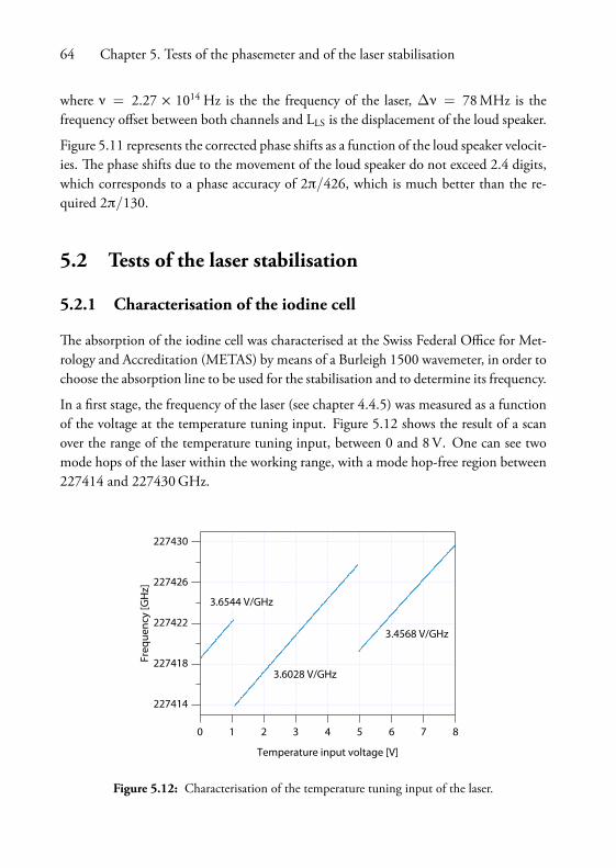
64 Chapter 5. Tests of the phasemeter and of the laser stabilisation
where ν = 2.27 × 10¹⁴ Hz is the the frequency of the laser, ∆ν = 78MHz is thefrequency offset between both channels and LLS is the displacement of the loud speaker.
Figure 5.11 represents the corrected phase shifts as a function of the loud speaker velocit-ies. e phase shifts due to the movement of the loud speaker do not exceed 2.4 digits,which corresponds to a phase accuracy of 2π/426, which is much better than the re-quired 2π/130.
5.2 Tests of the laser stabilisation
5.2.1 Characterisation of the iodine cell
e absorption of the iodine cell was characterised at the Swiss Federal Office for Met-rology and Accreditation (METAS) by means of a Burleigh 1500 wavemeter, in order tochoose the absorption line to be used for the stabilisation and to determine its frequency.
In a first stage, the frequency of the laser (see chapter 4.4.5) was measured as a functionof the voltage at the temperature tuning input. Figure 5.12 shows the result of a scanover the range of the temperature tuning input, between 0 and 8V. One can see twomode hops of the laser within the working range, with a mode hop-free region between227414 and 227430GHz.
Figure 5.12: Characterisation of the temperature tuning input of the laser.
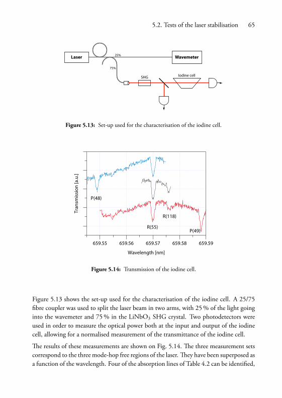
5.2. Tests of the laser stabilisation 65
25%
75%
Iodine cellSHG
Laser Wavemeter
Figure 5.13: Set-up used for the characterisation of the iodine cell.
Figure 5.14: Transmission of the iodine cell.
Figure 5.13 shows the set-up used for the characterisation of the iodine cell. A 25/75fibre coupler was used to split the laser beam in two arms, with 25% of the light goinginto the wavemeter and 75% in the LiNbO3 SHG crystal. Two photodetectors wereused in order to measure the optical power both at the input and output of the iodinecell, allowing for a normalised measurement of the transmittance of the iodine cell.
e results of these measurements are shown on Fig. 5.14. e three measurement setscorrespond to the three mode-hop free regions of the laser. ey have been superposed asa function of the wavelength. Four of the absorption lines of Table 4.2 can be identified,

66 Chapter 5. Tests of the phasemeter and of the laser stabilisation
Figure 5.15: Temperature scan of the laser, with an absorption of the iodine cell of about 7%.
the most promising one being R(55) as it is one of the strongest of the four and isconveniently located near the centre of the widest mode hop-free region of the laser.
As explained in chapter 4.4.3, the absorption of the iodine cell during these measure-ments was reduced to about 7% due to the condensation of the iodine in the cold fingerof the cell. However, the following measurements of the voltage sensitivity at the inputof the photodetector were performed with the modified cell heating and the expectedabsorption of 25%. Moreover, it was observed that at 25MHz, the voltage sensitivitySVP of the photodetector is only of 0.49V/µW instead of the expected 0.7 V/µW.
Figure 5.15 shows the first derivative of the transmission curve of the iodine cell over therange of the temperature tuning input of the laser (in blue), obtained by synchronouslydetecting the intensity at the output of the cell, as explained in chapter 4.2.3, along withthe corresponding frequency of the laser (in red). e slope of the signal at the centreof each absorption lines was calculated, giving the voltage sensitivity SVF. e valuefor the R(55) line is of 0.130V/GHz. It is better than the minimum required voltagesensitivity at the output of the photodetector calculated in chapter 4.2.3, but lower thanwhat could be expected from Eq. (4.12) in the current conditions.
Indeed, with an input power of Pin = 12 µW and a voltage sensitivity of the photo-detector of SVP = 0.49V/µW, the expected voltage sensitivity at the output of thephotodetector is of SVF = 0.412V/GHz. However, it was shown by Nicolas Schuhler

5.2. Tests of the laser stabilisation 67
and Samuel Lévêque at ESO that the absorption line is better approximated by a Gaus-sian function. In this case, the expected voltage sensitivity is of 0.266V/GHz. edifference can be caused by a frequency excursion of less than 80MHz in the EOM orby optical power losses between the SHG crystal and the detector.
5.2.2 Error signal monitoring
During the optimisation of the control loop, the easiest way to estimate whether the laserwas properly stabilised was by monitoring the error signal. Indeed, if the voltage sens-itivity at the output of the photodetector is known, the residual frequency fluctuationscan be calculated from the value of the error signal and the voltage sensitivity measuredwith a temperature scan of the laser.
However, it must be noted that this is not a measurement of the absolute stability of thesystem. Indeed, any external factor that affects the error signal will be corrected by thecontrol loop as if it were an error on the laser frequency.
Figure 5.16 shows the error signal for the laser in free running and in stabilised operation.Figure 5.17 shows the PSD of these measurements. One can see that the noise of thestabilised laser is below the required noise limit of 7.1 × 10⁴ Hz/
√Hz determined in
chapter 4.1.3.
Figure 5.16: Error signal in free-running (left) during 206minutes at a rate of 1Hz and in sta-bilised mode (right) during 39minutes at a rate of 1 kHz.

68 Chapter 5. Tests of the phasemeter and of the laser stabilisation
Figure 5.17: PSD of the error signal in free-running and in stabilised mode.
5.2.3 Test with long delay lines
e same test that was performed in chapter 4.1.2 to measure the frequency noise ofthe free running laser between 10Hz and 10 kHz was applied to the stabilised laser.e frequency fluctuations of the laser were deduced from the phase fluctuations of aninterferometer with a very large optical path difference achieved by a 1 km fibre delay.Figure 5.18 shows the set-up used.
+38 MHz
+38.65 MHz
Coupler
PC
Coupler
Coupler
Reference
Probe
1 km fibre delay
Figure 5.18: Set-up used for the test with long delay lines. PC: Polarisation controller.

5.2. Tests of the laser stabilisation 69
Figure 5.19: PSD of the frequency fluctuations of the free-running and stabilised laser.
Figure 5.19 shows the PSD of the frequency fluctuations of the free running and stabil-ised laser between 10Hz and 10 kHz. One can see that they are both below the requirednoise limit of 7.1 × 10⁴ Hz/
√Hz.
5.2.4 Further tests performed at ESO
After the stabilised laser was delivered to ESO, additional tests were performed by Nic-olas Schuhler and Samuel Lévêque that showed slow fluctuations of the laser frequencythat were outside the requirements. is section summarises the modifications that theymade to the system in order to correct this problem, as well as the results of the testsperformed to verify the performance of the improved stabilisation.
Redesign of the control loop
A new design for the control loop was introduced, in which two different PI controllersfor the piezo and temperature inputs of the laser operate almost independently. In orderto force the temperature loop to desaturate the piezo controller, the output of the piezoloop is added to the error signal at the input of the temperature loop, with a conversionfactor that takes into account the tuning rate of the piezo input of the laser and thevoltage sensitivity of the error signal.

70 Chapter 5. Tests of the phasemeter and of the laser stabilisation
Reduction of detection noise
As mentioned in chapter 5.2.2, any external factor that would affect the error signal(detection noise) would be interpreted as a variation of the laser frequency by the controlloop. ree sources of detection noise were identified at ESO:
• electronic crosstalk at 25MHz, originating from the cabling between the EOMand its driver;
• mechanical and acoustic vibrations affecting the 25/75 fibre coupler at the inputof the system;
• residual amplitude modulation (RAM) at the output of the EOM.
e electronic crosstalk was reduced with a clean recabling of the EOM. e fibrecoupler was removed and the dichroic filter is now used to collect the infrared lightand reinject it into an single-mode, polarisation-maintaining fibre for the PRIMA met-rology.
Part of the RAM could be reduced by adding a half-wave plate and a polariser at theinput of the EOM to allow a better matching of the polarisation of the incoming beamwith the axes of the EOM crystal. It was also determined that some RAM is intro-duced by a cavity effect in the crystal, whose length and refractive index change with thetemperature [15]. Tests were made by regulating the temperature of the EOM, but noimprovement was measured. Moreover, it was calculated that the temperature stabilityrequired to significantly reduce RAM due to the cavity effect is less than a tenth of adegree, which would add too much complexity to the system.
Tests with an optical frequency comb
e stabilised laser was brought to theMax Planck Institute forQuantumOptics (MPQ),Garching beiMünchenwho developed, through the firmMenloSystems, a self-referencedoptical frequency comb generator [16], which provides extremely stable frequency ref-erences in a wavelength range between one and two micrometres. ese tests of thefrequency stability of the laser were performed with the help of Dr Ronald Holzwarth,form MPQ and MenloSystems.
A beat signal was generated between the frequency comb and the stabilised laser and wasmeasured with a counter over 18 hours. Figure 5.20 shows the fluctuations of the beat

5.2. Tests of the laser stabilisation 71
Figure 5.20: Fluctuations of the beat frequency between the frequency comb and the Nd:YAGlaser (left) and PSD of the signal (right).
frequency and the PSD of the signal. e standard deviation is 808 kHz, which is belowthe specification of 2.2MHz.
72 Chapter 5. Tests of the phasemeter and of the laser stabilisation

Chapter 6
Conclusion
Digital phasemeter for superheterodyne detection
A differential phase detection system for the PRIMA instrument of the Very Large Tele-scope Interferometer has been developed based on superheterodyne interferometry. etarget accuracy was of 5 nm, with 1 nm resolution over a range of 100mm and 20 nW ofoptical power. e heterodyne frequencies of 450 kHz and 650 kHz required to obtaina 200 kHz superheterodyne frequency were generated with four fibre-pigtailed acousto-optic modulators.
A superheterodyne detection module has been developed, that performs optical detec-tion as well as electronic filtering and mixing of the heterodyne signals. e photode-tectors have a sensitivity of 1.23V/µW, a bandwidth of 7.7MHz and a noise below−128 dBm/Hz. With a 55 kHz bandwidth and the minimum optical power of 20 nW,it corresponds to a signal-to-noise ratio of 55 dB, which is well over the required SNRof 40 dB. e input bandpass filters at 450 kHz and 650 kHz have a phase responsethat has been matched to 0.42 within the ±55 kHz bandwidth, resulting in a distanceerror of about 0.8 nm between the reference and science channels. is error is belowthe target resolution of the phasemeter. e SNR of the superheterodyne module wasmeasured to be over 58 dB for electric signals equivalent to an optical power of 20 nW.e SNR was above the required 40 dB for equivalent optical powers as low as 0.2 nW.
A digital phasemeter based on Altera programmable logic devices has been designed. Ituses a 200MHz clock generated from the 200 kHz reference heterodyne signal by means
73

74 Chapter 6. Conclusion
of a phase-locked loop, resulting in a 2π/1024 phase resolution for a single measure-ment. It features a 19-bit integer fringe counter allowing for a range of 346mm andcan average phase data for arbitrary output rates between 0.5Hz and 8 kHz. e rmsresolution of the digital phasemeter was measured to be 2π/1678 over 4000 samples,corresponding to a distance of 0.4 nm. e required resolution was 2π/660. Tests ofaccuracy using two-wavelength interferometry on the phasemeter prototype showed anaccuracy of 2π/850. Dynamic tests reported a phase accuracy in common mode of2π/426 for delay line velocities between ±12mm/s, which is better than the requiredaccuracy of 2π/130.
Frequency stabilisation of a Nd:YAG laser
A set-up for the frequency stabilisation on iodine of a Nd:YAG laser at 1319 nm hasbeen designed. e requirements are for a long-term frequency stability and calibrationof 10−8 or 2.26MHz. e second harmonic of the laser at 659.5 nm was generated byquasi-phase matching in a periodically-poled Lithium Niobate crystal. For an opticalpower of 50mW in the fundamental beam focussed to 51.5 µm in the centre of the20mm long crystal, a second-harmonic power of 12 µW was obtained, correspondingto an efficiency of 2.4 × 10⁻⁴.
Frequency modulation of the laser light, synchronous detection and a digital controlloop are used to stabilise the laser frequency on the centre of an absorption line of iodine.e high frequency fluctuations are compensated by a Proportional-Integral regulatoracting on the piezo input of the laser. A second PI regulator is used to desaturate thepiezo actuator. Tests with an interferometer of large OPD (1 km fibre delay) showed thatthe frequency fluctuations between 10Hz and 10 kHz are below the required noise limitof 7.1 × 10⁴ Hz/
√Hz. Beat frequency measurements of the stabilised laser with a self-
referenced optical frequency comb generator at the Max Planck Institute for QuantumOptics demonstrated a stability of 808 kHz over 18 hours.
Future work
Following the work presented in this thesis, a new project between the European South-ern Observatory, Haute École Arc Ingénierie, and the Institute of Microtechnology hasbegun. It aims at improving the PRIMA laser metrology by means of an absolute met-rology system based on multiple-wavelength interferometry [17].

75
Several lasers are stabilised on an optical frequency comb (FC1500, MenloSystems)provided by a mode-locked laser with appropriate frequency differences in order to gen-erate the desired synthetic wavelengths. A new phasemeter for multiple-wavelength in-terferometry based on superheterodyne detection is also being developed.
Such an absolute metrology could reduce the complexity of the internal optical pathcalibration scheme of the VLTI and lead to an accurate determination of the baselinelength, thus increasing the overall performance of PRIMA.

76 Chapter 6. Conclusion

Acknowledgements
Now comes the time to thank people, and I would therefore like to thank a number ofpeople who know where their towel is [42].
First of all I would like to thank Professor René Dändliker for welcoming me into hislaboratory, giving me the opportunity of doing a PhD under his supervision, closelyfollowing my work and always being present when I needed his advice or support.
Yves Savadé, who has been my supervisor throughout the project, for everything hetaught me. I’m also especially grateful for his continuing availability even after he leftthe group.
Marcel Groccia, who designed and realised the analogue electronics and helped me a lotwith the digital electronics as well as with my sadly necessary dealings in the underworldof Windows PCs.
Ali Pourzand, who worked with me on the laser stabilisation. Working in the lab wasmuch more fun when he was there, even when results were off by a factor of π2. Also,I need to apologise to him for losing the Magic Hex Wrench, I’m afraid it was eaten bythe Floor Kraken.
From ESO I would like to thank Samuel Lévêque, who was responsible for my project,he was always open to discussion, spotting the critical issues and providing useful feed-back, and Nicolas Schuhler whose assistance has been very helpful during the design andtesting of the system.
Also from ESO, Philippe Duhoux for his precious help on interfacing with the VLToperation software,MartinDimmler for his advice on the design of the digital board, andalso Frédéric Dérie, Françoise Delplancke, Andreas Glindemann and ReinhardWilhelmfor their involvement in the project.
77

78 Acknowledgements
From METAS, Rudolf almann and Jacques Morel for their help with the character-isation of the laser.
From the Applied Optics Group I would especially like to thank Iwan Märki, who de-fended his thesis the same week as I did, for his support during the home straight, hisfriendship, all our serious, not so serious and downright not serious discussions and alsofor taking me on an unforgettable and adventurous trip to a beautiful local maximumof our country.
Special thanks are in order for Wataru Nakagawa, who was always availble for me as acolleague, a mentor and a friend and tought me a lot, work-related and other.
Sylvain Jaquet with whom I shared an office for quite some time, for his friendship andhis support and for constantly nagging me about the fact that there was no fog in LaChaux-de-Fonds when we were choking from it in Neuchâtel.
Patrick Ruffieux, a true biker with a chain drive on his bike, not one of those sissies whoprefer drive shafts because they’re low maintenance and give a smooth ride.
Olivier Ripoll, who was my assistant when I did my semester work, which gave me theopportunity to appreciate the good ambience in the lab.
Also Piero Tortora, Omar Manzardo, Martin Salt, Felix Schädelin and the rest of theApplied Optics Group, for the good atmosphere and interesting discussions.
e members of the jury, René Dändliker, Hans Peter Herzig, éo Lasser, SamuelLévêque and Yves Salvadé.
Finally I would like to thank my family, for they encouragements throughout my studiesand my scientific career, right from the beginning when I was a kid dreaming to becomean inventor.

Bibliography
[1] F. Delplancke, S. A. Lévêque, P. Kervella, A. Glindemann and L. D’Arcio, “Phase-referenced imaging and micro-arcsecond astrometry with the VLTI,” in P. J. Lenaand A. Quirrenbach, eds., “Interferometry in Optical Astronomy,” vol. 4006, pp.365–376, SPIE (2000).
[2] S. A. Lévêque, R. Wilhelm, Y. Salvadé, O. Scherler and R. Dändliker, “Towardnanometer accuracy laser metrology for phase-referenced interferometry with theVLTI,” in W. A. Traub, ed., “Interferometry for Optical Astronomy II,” vol. 4838,pp. 983–994, SPIE (2003).
[3] R. Dändliker, R. almann and D. Prongué, “Two-wavelength laser interfero-metry using superheterodyne detection,” Opt. Lett. 13 (5), 339–341 (1988).
[4] Y. Salvadé and R. Dändliker, “Limitations of interferometry due to the flicker noiseof laser diodes,” J. Opt. Soc. Amer. A 17 (5), 927–932 (2000).
[5] T. Dennis, E. A. Curtis, C. W. Oates, L. Hollberg and S. L. Gilbert, “Wavelengthreferences for 1300-nm wavelength-division multiplexing,” J. Lightwave Technol.20 (5), 776–782 (2002).
[6] A. Arie, M. L. Bortz, M. M. Fejer and R. L. Byer, “Iodine spectroscopy and abso-lute frequency stabilization with the second-harmonic of the 1319-nm Nd:YAGlaser,” Opt. Lett. 18 (20), 1757–1759 (1993).
[7] R. V. Pound, “Electronic frequency stabilization of microwave oscillators,” Rev. Sci.Inst. 17 (11), 490–505 (1946).
79

80 Bibliography
[8] R. W. P. Drever, J. L. Hall, F. V. Kowalski, J. Hough, G. M. Ford, A. J. Munleyand H.Ward, “Laser phase and frequency stabilization using an optical-resonator,”Appl. Phys. B 31 (2), 97–105 (1983).
[9] A. Yariv and P. Yeh, Optical Waves in Crystals, John Wiley & Sons, Inc. (1984).
[10] A. Yariv, Optical Electronics, CBS College Publishing, 3rd ed. (1985).
[11] A. K. Ghatak and K. yagarajan, Optical Electronics, Cambridge University Press(1989).
[12] B. Boulanger, J. P. Feve and Y. Guillien, “ermo-optical effect and saturation ofnonlinear absorption induced by gray tracking in a 532-nm-pumped KTP opticalparametric oscillator,” Opt. Lett. 25 (7), 484–486 (2000).
[13] F. C. Zumsteg, J. D. Bierlein and T. E. Gier, “KxRb1−xTiOPO4: A new nonlinearoptical material,” J. Appl. Phys. 47 (11), 4980–4985 (1976).
[14] Y. Salvadé, Distance Measurement by Multiple-Wavelength Interferometry, Ph.D.thesis, Université de Neuchâtel (1999).
[15] E. A.Whittaker, M.Gehrtz andG.C. Bjorklund, “Residual amplitudemodulationin laser electro-optic phase modulation,” J. Opt. Soc. Amer. B 2, 1320 (1985).
[16] D. J. Jones, S. A. Diddams, J. K. Ranka, A. Stentz, R. S. Windeler, J. L. Hall andS. T. Cundiff, “Carrier-envelope phase control of femtosecond mode-locked lasersand direct optical frequency synthesis,” Science 288 (5466), 635–639 (2000).
[17] Y. Salvadé, A. Courteville and R. Dändliker, “Absolute metrology for the VeryLarge Telescope Interferometer (VLTI),” in P. J. Lena and A. Quirrenbach, eds.,“Interferometry in Optical Astronomy,” vol. 4006, pp. 424–431, SPIE (2000).
[18] S. Lévêque, Y. Salvadé, R. Dändliker and O. Scherler, “High-accuracy laser met-rology enhances the VLTI,” Laser Focus World 38 (4), 101–104 (2002).
[42] e Hitchhiker’s Guide to the Galaxy, Megadodo Publications, Light City, UrsaMinor Beta.