high performance conflict detection and resolution for
TRANSCRIPT

High Performance Conflict Detection andResolution for
Multi-Dimensional Objects
Von der Fakultät für Elektrotechnik und Informatikder Gottfried Wilhelm Leibniz Universität Hannover
zur Erlangung des GradesDoktor der Naturwissenschaften
Dr. rer. nat.genehmigte Dissertation von
Dipl.-Inform. Alexander Kuenzgeboren am 08.09.1974 in Bad Harzburg
2015

1. Referent . . . . . . . . . . . . . . . . . . . . . . . . . Prof. Dr. Franz-Erich Wolter2. Referent . . . . . . . . . . . . . . . . . . . . . . . . . . . . . . . . Prof. Dr. Dirk Kügler3. Referent . . . . . . . . . . . . . . . . . . . . . . . . . Prof. Dr. Gabriel ZachmannTag der Promotion . . . . . . . . . . . . . . . . . . . . . . . . . . . . . . . . . . . 20.07.2015

Preliminary Publications
Some ideas and figures have appeared previously in the followingpublications:
Patents
Kuenz, A. and N. Peinecke (2011, February). Effiziente 4D-Konflikt-Erkennung für großräumige Szenarien, Verfahren zur Ermittlungeiner potenziellen Konfliktsituation. Patent (EP 2 457 224 A2).Kuenz, A. and N. Peinecke (2012, June). Method for determining apotential conflict situation. Patent (US 20120158278).
Publications
Kuenz, A. (2014). Increasing the margins - more freedom intrajectory-based operations. In Proc. IEEE/AIAA 33rd DigitalAvionics Systems Conf. DASC 2014. (Best Paper of Session)Kuenz, A., G. Schwoch, and F.-E. Wolter (2013, October). Indi-vidualism in global airspace - user preferred trajectories in futureATM. In Proc. IEEE/AIAA 32nd Digital Avionics Systems Conf.DASC 2013. (Best Paper of Track)Kuenz, A. and G. Schwoch (2012, October). Global time-basedconflict solution: towards the overall optimum. In Proc. IEEE/AIAA31st Digital Avionics Systems Conf. DASC 2012.Kuenz, A. (2012, June). Optimizing tomorrows ATM using 4D-trajectory-based operations. In ODAS 2012.Kuenz, A. (2011, October). A global airspace model for 4D-trajec-tory-based operations. In Proc. IEEE/AIAA 30th Digital AvionicsSystems Conf. DASC 2011. (Best Paper of Session)Kuenz, A. and N. Peinecke (2009, October). Tiling the world -efficient 4D conflict detection for large scale scenarios. In Proc.IEEE/AIAA 28th Digital Avionics Systems Conf. DASC 2009.

Abstract
4D-trajectory based operations is one of the big enabler for fu-ture high-capacity, efficient and environmentally friendly air trafficmanagement. Every aircraft is scheduled to fly along a predicted4D path that can be calculated from gate to gate pre-flight. 4D-trajectories are optimized individually for aircraft taking into ac-count performance models, routes, weather conditions and airlinepreferences. However, individual calculation of trajectories doesnot ensure conflict-freeness with surrounding traffic. This workdescribes an efficient algorithm detecting conflicts for large trafficscenarios. Conflict detection is performed between aircraft trajecto-ries, also taking into account environmental constraints like severeweather zones and restricted areas. Basic idea is an N -dimensionalbisection of airspace allowing a significant reduction of complexity.Thus, potential conflicts are identified very fast. A slower highprecision conflict check is performed on potential conflicts only.On average, conflicts of one 4D-trajectory can be detected in aEuropean traffic sample holding more than 33 000 flights in lessthan 2.5 ms on standard PC hardware.Fast detection times are predestined for trial-and-error conflictresolution. Different conflict resolution methods are illustrated,taking into account the major key performance areas in air traf-fic management, e. g., safety, efficiency, and predictability. As anexample, deconfliction is performed on an optimized version ofaforementioned European traffic sample holding 33 000 flights.
Keywords: Conflict Detection and Resolution, 4D-Trajectory-Based Operations, N -dimensional Bisection

Zusammenfassung
Ein wichtiger Bestandteil kapazitätserhöhender, effizienter undumweltfreundlicher Zukunftskonzepte im Luftverkehrsmanagementsind 4D-Trajektorien. Jedes Luftfahrzeug fliegt in einem derarti-gen Szenario entlang einer 4D-Flugbahn, die bereits vor dem Startfür den gesamten Flugweg berechnet werden kann. Diese Flugbah-nen werden von Fluggesellschaften individuell für Flugzeugmuster,Routen und Wetterbedingungen optimiert. In einem gemeinsamenLuftraum sind individuell berechnete Trajektorien jedoch in derRegel nicht konfliktfrei. Diese Arbeit beschreibt einen effizientenAlgorithmus zur Erkennung von Konflikten in sehr großen Szena-rien. Die Konfliktidentifizierung erkennt Annäherungen zwischenVerkehrsteilnehmern sowie Verletzungen von Beschränkungsgebie-ten wie Schlechtwetter- und Flugverbotszonen. Die Grundidee isteine N -dimensionale Bisektion des Luftraums zur signifikanten Re-duktion der Gesamtkomplexität. Durch dieses Verfahren werdenpotenzielle Konflikte sehr schnell identifiziert. Ein präziser und lang-samerer Algorithmus zur finalen Entscheidung wird lediglich auf denzuvor identifizierten potenziellen Konflikten durchgeführt. In einemEuropäischen Verkehrsszenario mit mehr als 33 000 Flugzeugen kön-nen mit Hilfe des Algorithmus alle Konflikte einer 4D-Trajektorie imMittel in weniger als 2.5 ms auf Standard-PC-Hardware identifiziertwerden.Die geringen Antwortzeiten erlauben, dass über intelligente Versuch-und-Irrtum-Verfahren effizient Konfliktlösungsstrategien umgesetztwerden können. Für den 4D-Flugverkehr werden Lösungsstrategienaufgezeigt, die neben der Konfliktfreiheit noch andere Faktoren wieEffizienz, Emissionsvermeidung und Planbarkeit berücksichtigen.Beispielhaft werden Lösungsalgorithmen auf eine optimierte Varian-te des zuvorgenannten Europäischen Verkehrsszenarios mit 33 000Flügen angewendet.
Schlagworte: Konflikterkennung und -lösung, 4D-trajektorienba-sierte Konzepte, N -dimensionale Bisektion


Acknowledgements
This work would not have been possible without the support ofseveral people, to whom I am greatly indebted.
First of all, I like to thank Prof. Dr. Franz-Erich Wolter foraccepting to supervise my thesis. He always gave me good adviceand support.
I am also grateful to my head of institute Prof. Dr. Dirk Küglerfor taking over co-advisorship. Furthermore, he and my head ofdepartment, Dr. Bernd Korn, provided me with a great workingenvironment at DLR’s Institute of Flight Guidance and tolerated myresearch on conflict detection and avoidance even without directlyfeeding into a project from the beginning.
I also would like to thank Prof. Dr. Gabriel Zachmann for hiskind willingness to be third accessor.
At DLR, I had (and still have) very nice fellows supporting thecompletion of my thesis. Without claim to be complete, I thankDr. Niklas Peinecke for co-authoring my patent on conflict detectionand initiating the link to my supervisor, Christiane Edinger fordeveloping the highly sophisticated Advanced Flight ManagementSystem I used as trajectory prediction engine, Gunnar Schwochfor preparing optimized traffic scenarios, and Ralf Kohrs and UweTeegen for proof-reading. More generally, I thank all participantsof the coffee breaks of department FL23 for endless, all-embracing,

and very fruitful discussions on many details of this work. I amgrateful to everyone using the NDMap-implementation, extendingthe field of application, pointing me to problems, and requestinginteresting new features.
Last but not least, my thanks go to my wife Anja and mychildren Leonard and Annelie for accepting countless working hoursin the evenings and weekends for writing this thesis.

Contents
Acronyms 7
Symbols 11
1 Introduction 23
2 Related Work 272.1 Mathematics and Algorithms . . . . . . . . . . . . . 27
2.1.1 Bisection . . . . . . . . . . . . . . . . . . . . 282.1.2 Binary Tree . . . . . . . . . . . . . . . . . . . 282.1.3 Binary Space Partitioning Tree . . . . . . . . 282.1.4 k-dimensional Tree . . . . . . . . . . . . . . . 302.1.5 R-Tree . . . . . . . . . . . . . . . . . . . . . . 30
2.2 Conflict Detection Mechanisms . . . . . . . . . . . . 322.2.1 Multiple Phases for Complex Scenarios . . . 332.2.2 Discrete and Continuous Motion . . . . . . . 332.2.3 Convex Polygon Intersection . . . . . . . . . 342.2.4 Simple Polygon Intersection . . . . . . . . . . 35
1

2 CONTENTS
2.2.5 Plane Sweep Algorithms . . . . . . . . . . . . 362.2.6 Intersection and Range Searching . . . . . . . 372.2.7 Bounding Volume Hierarchy . . . . . . . . . . 382.2.8 Kinetic Data Structures . . . . . . . . . . . . 412.2.9 Sweep and Prune . . . . . . . . . . . . . . . . 432.2.10 Broad Phase Based on Delaunay Triangulation 442.2.11 Spatial Subdivision . . . . . . . . . . . . . . . 442.2.12 Spatial Hashing . . . . . . . . . . . . . . . . . 44
2.3 4D Trajectory Prediction . . . . . . . . . . . . . . . 462.3.1 The Advanced Flight Management System . 48
2.4 Conflict Detection in Aviation . . . . . . . . . . . . . 582.4.1 Conflict Situations in Aviation . . . . . . . . 59
2.4.1.1 Sector Load and Flow Control Con-flicts . . . . . . . . . . . . . . . . . . 60
2.4.1.2 Trajectory Based Conflicts . . . . . 602.4.1.3 Medium-Term Conflict Detection . . 612.4.1.4 Short-Term Conflict Alert . . . . . . 612.4.1.5 Airborne Collision Avoidance System 61
2.4.2 Trajectory-Based Conflict Detection . . . . . 622.4.3 Subdivision of Airspace . . . . . . . . . . . . 632.4.4 Conflict Detection Considering Uncertainty . 65
2.5 Conflict Resolution in Aviation . . . . . . . . . . . . 672.5.1 Conflict Resolution using Trial-and-Error . . 692.5.2 Conflict Resolution using Genetic Algorithm 702.5.3 Conflict Resolution based on Potential Fields 712.5.4 Conflict Resolution based on Light Propagation 722.5.5 Conflict Avoidance in Crowd Simulation . . . 722.5.6 Extended Flight Rules . . . . . . . . . . . . . 73
2.6 Geodetic Earth Systems . . . . . . . . . . . . . . . . 73

CONTENTS 3
2.6.1 Distances on Earth . . . . . . . . . . . . . . . 762.6.2 Map Projection . . . . . . . . . . . . . . . . . 77
2.6.2.1 Sinusoidal Projection . . . . . . . . 772.6.2.2 Mercator Projection . . . . . . . . . 772.6.2.3 Transverse Mercator Projection . . 78
3 Conflict Detection 813.1 Definitions . . . . . . . . . . . . . . . . . . . . . . . . 833.2 N-Dimensional Conflict . . . . . . . . . . . . . . . . 87
3.2.1 Conflicts without Time Reference . . . . . . . 883.2.2 Conflicts with Time Reference . . . . . . . . 88
3.3 N-Dimensional Tiling Algorithm . . . . . . . . . . . 893.3.1 Affected Tiles . . . . . . . . . . . . . . . . . . 923.3.2 Check for Penetration . . . . . . . . . . . . . 933.3.3 Check for Vicinity . . . . . . . . . . . . . . . 953.3.4 Symmetric Simplification . . . . . . . . . . . 973.3.5 Full Containment . . . . . . . . . . . . . . . . 983.3.6 Bounding Boxes . . . . . . . . . . . . . . . . 993.3.7 Building the Tree . . . . . . . . . . . . . . . . 1013.3.8 Monotonic Dimensions . . . . . . . . . . . . . 1023.3.9 Balancing the Tree . . . . . . . . . . . . . . . 1023.3.10 Broad Phase vs. Narrow Phase . . . . . . . . 1043.3.11 Memory Limitation . . . . . . . . . . . . . . 1053.3.12 Tile Knowledge . . . . . . . . . . . . . . . . . 105
3.4 Supported Objects . . . . . . . . . . . . . . . . . . . 1063.4.1 N-Dimensional Trajectories . . . . . . . . . . 1063.4.2 N-Dimensional Volumes . . . . . . . . . . . . 1073.4.3 N-Dimensional Moving Volumes . . . . . . . 109
3.5 N-Dimensional Conflict Detection . . . . . . . . . . . 113

4 CONTENTS
3.5.1 Conflict between Trajectories . . . . . . . . . 1163.5.1.1 Trajectory Conflict including Time
Reference . . . . . . . . . . . . . . . 1163.5.1.2 Trajectory Conflict without Time
Reference . . . . . . . . . . . . . . . 1173.5.2 Conflict between Trajectory and Volume . . . 118
3.5.2.1 Trajectory/Volume Conflict includ-ing Time Reference . . . . . . . . . 118
3.5.2.2 Trajectory/Volume Conflict with-out Time Reference . . . . . . . . . 118
3.5.3 Conflict Merging . . . . . . . . . . . . . . . . 1183.5.4 Output Format . . . . . . . . . . . . . . . . . 119
3.6 Objects in Focus . . . . . . . . . . . . . . . . . . . . 1213.7 Software Implementation . . . . . . . . . . . . . . . . 121
4 CD in 4D-Airspace 1254.1 Topological Isomorphism of Earth . . . . . . . . . . 126
4.1.1 The Earth-Mode . . . . . . . . . . . . . . . . 1264.1.2 Great Circle Connections . . . . . . . . . . . 1294.1.3 Singularity and Discontinuity of Longitudes . 1314.1.4 Alternative Earth Mapping . . . . . . . . . . 134
4.1.4.1 Spherical Coordinate System . . . . 1344.1.4.2 Geodesic Dome . . . . . . . . . . . . 136
4.2 Traffic Samples and Conditions . . . . . . . . . . . . 1374.2.1 German Traffic Sample . . . . . . . . . . . . 1374.2.2 European Traffic Sample . . . . . . . . . . . . 139
4.3 Results from Conflict Detection . . . . . . . . . . . . 1414.4 Performance Indicators . . . . . . . . . . . . . . . . . 145
4.4.1 Number of Trajectories . . . . . . . . . . . . 1454.4.2 Density of Trajectories . . . . . . . . . . . . . 147
CONTENTS 5
4.4.3 Number of Trajectory Sampling Points . . . . 147
4.4.4 Length of Trajectories . . . . . . . . . . . . . 148
4.4.5 Number of Potential and Real Conflicts . . . 148
4.4.6 Summary of Performance Indicators . . . . . 148
4.5 Performance Optimization for CD . . . . . . . . . . 148
4.5.1 Lateral Tile Size Optimization . . . . . . . . 149
4.5.2 Vertical Tile Size Optimization . . . . . . . . 149
4.5.3 Time-based Tile Size Optimization . . . . . . 151
4.5.4 Balancing the Tree . . . . . . . . . . . . . . . 152
4.5.5 Focus on Aircraft . . . . . . . . . . . . . . . . 156
4.5.6 Shrinking the Root Tile . . . . . . . . . . . . 157
4.6 Comparison with Octrees . . . . . . . . . . . . . . . 159
4.7 Application in Projects . . . . . . . . . . . . . . . . . 161
4.7.1 Future Air Ground Integration . . . . . . . . 161
4.7.2 Luftraummanagement 2020 . . . . . . . . . . 163
4.7.3 Volcanic Ash Impact on the Air TransportSystem . . . . . . . . . . . . . . . . . . . . . 164
4.7.4 Supercooled Large Droplets Icing . . . . . . . 167
4.7.5 4 Dimensional-Contracts - Guidance and Con-trol . . . . . . . . . . . . . . . . . . . . . . . 168
5 4D Conflict Resolution 171
5.1 Global Trial-and-Error CR . . . . . . . . . . . . . . . 172
5.2 Lateral Resolution . . . . . . . . . . . . . . . . . . . 175
5.3 Vertical Resolution . . . . . . . . . . . . . . . . . . . 177
5.4 Time-Based Resolution . . . . . . . . . . . . . . . . . 178
5.4.1 Moving Whole Flights in Time . . . . . . . . 179
5.4.1.1 Global Algorithm . . . . . . . . . . 180
5.4.1.2 Recursive Algorithm . . . . . . . . . 181

6 CONTENTS
5.4.2 Flight Duration Adaptation . . . . . . . . . . 1835.5 Deconflicting Optimized Traffic . . . . . . . . . . . . 183
5.5.1 Airport-Focused Conflict Resolution . . . . . 1875.5.2 Global Conflict Resolution . . . . . . . . . . . 1885.5.3 Resolution of En-Route Conflicts . . . . . . . 190
6 Verification and Validation 1936.1 Nominal Case . . . . . . . . . . . . . . . . . . . . . . 1946.2 Pseudo-Parallel Case . . . . . . . . . . . . . . . . . . 1946.3 Conflict Jitter Case . . . . . . . . . . . . . . . . . . . 1986.4 Singularity Case . . . . . . . . . . . . . . . . . . . . 2016.5 Discontinuity Case . . . . . . . . . . . . . . . . . . . 2026.6 Polygon Volume Case . . . . . . . . . . . . . . . . . 205
7 Conclusions and Outlook 209
8 Update after Disputation 2158.1 Conflict Metric . . . . . . . . . . . . . . . . . . . . . 2158.2 Performance . . . . . . . . . . . . . . . . . . . . . . . 216
Acronyms
4DCo-GC 4 Dimensional-Contracts - Guidance and Con-trol
AABB Axes Aligned Bounding BoxACAS Airborne Collision Avoidance SystemADS-B Automatic Dependent Surveillance-BroadcastAFMS Advanced Flight Management SystemANS Air Navigation ServiceAOC Airline Operation CenterArr ArrivalATC Air Traffic ControlATCo Air Traffic ControllerATM Air Traffic ManagementATRA Advanced Technology Research AircraftATTAS Advanced Technologies Testing Aircraft System
BADA Base of Aircraft DAtaBSP Binary space partitioningBVH Bounding Volume Hierarchy
CAS Calibrated Air SpeedCDA Continuous Descent ApproachCFMU Central Flow Management Unit
7

8 Acronyms
CGAL Computational Geometry Algorithms LibraryClb ClimbCPA Closest Point of ApproachCPU Central Processing UnitCrs CruiseCTAS Center-TRACON Automation System
DDR Demand Data RepositoryDep DepartureDFS DFS Deutsche Flugsicherung GmbHDLR Deutsches Zentrum fuer Luft- und Raumfahrt
(German Aerospace Center)dops Discrete Orientation PolytopesDsc DescentDWD Deutscher Wetterdienst
E-TMA Extended TMAEFR Extended Flight RulesENU East-North-UpERAT Environmentally Responsible Air TransportEurocontrol European Organisation for the Safety of Air
Navigation
FACTS Future Aeronautical Communications TrafficSimulator
FAGI Future Air Ground IntegrationFL Flight LevelFMS Flight Management SystemFP7 Seventh Framework Programme for Researchft feet
Glonass Globalnaja Nawigazionnaja Sputnikowaja Sis-tema
GPS Global Positioning System
ICAO International Civil Aviation OrganizationIFR Instrument Flight Rules
k-d tree k-dimensional tree

Acronyms 9
KDS Kinetic Data StructureKML Keyhole Markup LanguageKPA Key Performance Areaskts knots
LAnAb Leise An- und AbflügeLDLP Low Drag Low PowerLRM2020 Luftraummanagment 2020
MTCD Medium Term Conflict Detection
NDMap N-Dimensional Map-ImplementationNextGen Next GenerationNM Nautical Miles
PHARE Programme for Harmonised Air Traffic Man-agement Research in Eurocontrol
SCDA Segmented Continuous Descent ApproachSESAR Single European Sky ATM ResearchSLD Supercooled Large DropletSSR Secondary Surveillance RadarSTCA Short Term Conflict AlertSuLaDI Supercooled Large Droplets Icing
TBO Trajectory Based OperationsTMA Terminal Maneuvering AreaTOD Top Of DescentTRACON Terminal Radar Approach Control
VFW Vereinigte Flugtechnische WerkeVLSI Very-large-scale integrationVolcATS Volcanic ash impact on the Air Transport Sys-
temVR Virtual RealityVTS Vertical Tile Size
WGS84 World Geodetic System 1984

10 Acronyms
ZFB Zentrum für Flugsimulation Berlin

Symbols
A N-dimensional tile�amax Maximum tile values for each dimension N�amin Minimum tile values for each dimension Na Equatorial radius of Earth ellipsoidBO Axis aligned Bounding Box of Object Ob Polar distance from center of Earth ellipsoid�D Number of necessary subdivisions in R
N
f Flattening of Earth ellipsoidG Minimum gap time between two conflictsλ LongitudeL(�p1, �p2) Line segment from �p1 to �p2N Dimension in N
O Object. Either trajectory or volumeP 2D-Polygonϕ Latitude�p Point in R
N
�S Mandatory separation in RN
S Simplex in RN
T Trajectory objectτ Common timeti Trajectory instancesV Polygon Volume, implementation of volume ob-
ject
11

12 Symbols
V Volume object

List of Figures
1.1 En-Route Metrics for Airborne Conflicts . . . . . . . 25
2.1 Quad Tree Example . . . . . . . . . . . . . . . . . . 29
2.2 k-d Tree Example . . . . . . . . . . . . . . . . . . . . 31
2.3 R-Tree Example . . . . . . . . . . . . . . . . . . . . 32
2.4 Intersection Calculation between two Convex Polygons 35
2.5 Eliminating Half of at least one Vertex Chain . . . . 36
2.6 Four Types of Intersection according to Edelsbrunnerand Maurer (1981) . . . . . . . . . . . . . . . . . . . 38
2.7 ATTAS Cockpit allowing 3 Ways of Flying . . . . . 47
2.8 DLR’s former Research Aircraft ATTAS . . . . . . . 48
2.9 In- and Outputs of AFMS . . . . . . . . . . . . . . . 49
2.10 Approach Types supported by AFMS . . . . . . . . 50
2.11 Calculating the TOD . . . . . . . . . . . . . . . . . . 51
2.12 CDA Trajectory for Airbus A330-300 . . . . . . . . . 52
2.13 Noise Footprint of LDLP . . . . . . . . . . . . . . . 54
2.14 Noise Footprint of CDA . . . . . . . . . . . . . . . . 55
13

14 LIST OF FIGURES
2.15 CDA flown by ATTAS . . . . . . . . . . . . . . . . . 562.16 CDA flown by Airbus A330-300 . . . . . . . . . . . . 572.17 Example Grid with Conflict according to Koeners
and de Vries (2008) . . . . . . . . . . . . . . . . . . . 642.18 Conflict in Octree between V1 and V2 according to
Hildum and Smith (2004) . . . . . . . . . . . . . . . 652.19 Trajectory Prediction Error Ellipses according to
Erzberger et al. (1997) . . . . . . . . . . . . . . . . . 662.20 Three Types of Conflict Resolution . . . . . . . . . . 682.21 Horizontal Resolution according to Erzberger et al.
(2010) . . . . . . . . . . . . . . . . . . . . . . . . . . 692.22 Vertical Resolution according to Erzberger et al. (2010) 692.23 Time-Based Resolution according to Erzberger et al.
(2010) . . . . . . . . . . . . . . . . . . . . . . . . . . 702.24 Point P with Latitude ϕ and Longitude λ . . . . . . 752.25 Sinusoidal Projection . . . . . . . . . . . . . . . . . . 782.26 Mercator Projection . . . . . . . . . . . . . . . . . . 782.27 Transverse Mercator Projection . . . . . . . . . . . . 79
3.1 Lateral Separation between 4D-Trajectories . . . . . 843.2 Vertical Separation between 4D-Trajectories . . . . . 843.3 Time-based Separation between 4D-Trajectories . . . 843.4 4D-Hypercube (Tesseract) . . . . . . . . . . . . . . . 843.5 Bisection for 1-3 Dimensions . . . . . . . . . . . . . . 913.6 First Level Bisection of Tesseract with 16 Children . 913.7 Objects in Different Tiles having a Lateral Conflict . 933.8 Trajectory in Fly-Through and Fly-By Zone . . . . . 963.9 No Conflict without Fly-Through Object in Center
Tile . . . . . . . . . . . . . . . . . . . . . . . . . . . 973.10 Two Trajectories in Conflict with the Volume German
Airspace . . . . . . . . . . . . . . . . . . . . . . . . . 99

LIST OF FIGURES 15
3.11 Axis Aligned vs. Object Oriented Bounding Box . . 1003.12 Shape Generated by Moving Polygon . . . . . . . . . 1113.13 Shape Generated by Less Symmetric Polygon . . . . 1113.14 3D-Corridor for Moving Polygon . . . . . . . . . . . 1123.15 Generation of Vertical Corridor . . . . . . . . . . . . 1133.16 Intersection between Moving Polygon and Tile Plane
marked with Red Sphere . . . . . . . . . . . . . . . . 1143.17 Two Non-conflicting Objects in same Tile . . . . . . 1153.18 Calculation of Start and End of Conflict . . . . . . . 1173.19 Discretization of Time prevents Gap Jump . . . . . 1193.20 12 Objects and their Conflicts . . . . . . . . . . . . . 1223.21 Focus on Objects 10-12 . . . . . . . . . . . . . . . . 122
4.1 Latitudes and Longitudes on Earth . . . . . . . . . . 1264.2 Spherical and Corresponding Cartesian Model . . . 1274.3 Cartesian vs. Great Circle Connection . . . . . . . . 1294.4 Influence of Distance and Latitude on Great Circle-
Cartesian Distance . . . . . . . . . . . . . . . . . . . 1304.5 Douglas-Peucker for Polygonal Approximation . . . . 1314.6 Shortest Connection on Spherical and Cartesian Rep-
resentation . . . . . . . . . . . . . . . . . . . . . . . 1324.7 Passing the Date Line in Cartesian Coordinates . . . 1334.8 Alternate Earth Mapping . . . . . . . . . . . . . . . 1344.9 Icosahedron with 4 Triangle Subdivision . . . . . . . 1364.10 Airborne Aircraft in German Traffic Sample . . . . . 1384.11 German Air Traffic Sample . . . . . . . . . . . . . . 1384.12 Optimized European Air Traffic Sample . . . . . . . 1384.13 Airborne Aircraft in European Traffic Sample . . . . 1394.14 Four Points in Worst Case for a Flyable Route Layout1414.15 Detection Times for German Sample Baseline . . . . 142

16 LIST OF FIGURES
4.16 Detection Times for German Sample Advanced Baseline142
4.17 Detection Times for German Sample with TilingAlgorithm . . . . . . . . . . . . . . . . . . . . . . . . 144
4.18 Detection Times for European Sample with TilingAlgorithm . . . . . . . . . . . . . . . . . . . . . . . . 145
4.19 Detection Times for Quadrupled German Scenario . 146
4.20 Detection Times for Increased Number of SamplingPoints . . . . . . . . . . . . . . . . . . . . . . . . . . 147
4.21 Variation of Tile Size . . . . . . . . . . . . . . . . . . 150
4.22 Variation of Altitude . . . . . . . . . . . . . . . . . . 151
4.23 Variation of Time . . . . . . . . . . . . . . . . . . . . 152
4.24 Results for 80 Seconds Tile Duration (Germany) . . 153
4.25 Results for 80 Seconds Tile Duration (Europe) . . . 153
4.26 Results from Automatically Balanced Tree . . . . . . 154
4.27 Results from Modified Balancing Algorithm . . . . . 155
4.28 Algorithm’s Performance for Different Numbers ofSelected Aircraft . . . . . . . . . . . . . . . . . . . . 156
4.29 Results from Shrunk Root Tile . . . . . . . . . . . . 157
4.30 3D-Octree Latitude/Longitude/Altitude . . . . . . . 160
4.31 3D-Octree Latitude/Longitude/Time . . . . . . . . . 160
4.32 The FAGI Concept . . . . . . . . . . . . . . . . . . . 163
4.33 Conflicts between Air Traffic and Volcanic Ash Cloud165
4.34 Vertical and Lateral De-Confliction from SLD-IcingArea . . . . . . . . . . . . . . . . . . . . . . . . . . . 168
4.35 Contract Definition in the 4DCo-GC Project . . . . 170
5.1 Lateral Resolution of Conflict . . . . . . . . . . . . . 176
5.2 Vertical Resolution of Conflict . . . . . . . . . . . . . 177
5.3 Time-Based Resolution of Conflict . . . . . . . . . . 178
5.4 Flights from/to Frankfurt-Main as XYT-Diagram 24h180

LIST OF FIGURES 17
5.5 Flights from/to Frankfurt-Main as XYT-Diagramaround Noon . . . . . . . . . . . . . . . . . . . . . . 181
5.6 Solving Conflicts Recursively . . . . . . . . . . . . . 1825.7 29k Conflicts in European Sample . . . . . . . . . . 1845.8 Conflicts per Flight . . . . . . . . . . . . . . . . . . . 1855.9 Conflicts in Vicinity of Munich (Example) . . . . . . 1855.10 Conflicts by Flight Phase . . . . . . . . . . . . . . . 1865.11 Conflicts after Shift of ±30 seconds . . . . . . . . . . 1875.12 Conflicts after Shift of ±10 minutes . . . . . . . . . . 1875.13 Airport-Focused Reduction in Relation to Time-Shift 1885.14 Recursive Optimization Level 10 . . . . . . . . . . . 1885.15 Recursive Optimization Level 20 . . . . . . . . . . . 1885.16 Global Reduction in Relation to Time-Shift . . . . . 1895.17 Conflicts after Global Shift of ±10 minutes . . . . . 1905.18 Global Recursion Optimization Level 20 . . . . . . . 1905.19 Conflicts after Lateral and Vertical Resolution . . . . 1905.20 Very Short En-route Conflict in Red . . . . . . . . . 1905.21 Remaining Conflicts . . . . . . . . . . . . . . . . . . 191
6.1 Four Trajectories with Conflicts . . . . . . . . . . . . 1966.2 Pseudo-Parallel Trajectories . . . . . . . . . . . . . . 1986.3 Jitter in Conflict . . . . . . . . . . . . . . . . . . . . 2006.4 Conflict at North Pole . . . . . . . . . . . . . . . . . 2026.5 Conflicts at Date Line . . . . . . . . . . . . . . . . . 2046.6 Conflicts with Germany Volume . . . . . . . . . . . . 207
8.1 Improved Detection Times with New Data Structuresfor Europe . . . . . . . . . . . . . . . . . . . . . . . . 217
8.2 Improved Detection Times with New Data Structuresfor Geramy . . . . . . . . . . . . . . . . . . . . . . . 218

18 LIST OF FIGURES
List of Tables
2.1 Separation in [NM] Depending on Wake Categories . 58
2.2 Priority for Aircraft in Different Flight Phases(Duong et al., 1996) . . . . . . . . . . . . . . . . . . 74
2.3 Reference Ellipsoids for Earth . . . . . . . . . . . . . 76
3.1 Overview on N-dimensional Bisection . . . . . . . . . 90
3.2 Boundaries of N-dimensional Tiles . . . . . . . . . . 95
3.3 Root Tile covering one Day on Earth . . . . . . . . . 103
3.4 Balanced Root Tile holding one Day on Earth . . . . 103
3.5 Phase Merging of Conflict Types . . . . . . . . . . . 120
4.1 Setup of Conflict Map for 4D-Airspace . . . . . . . . 125
4.2 Properties of Traffic Samples . . . . . . . . . . . . . 143
4.3 Vertical Dimension with Increased Vertical Tile Size 150
4.4 Time Dimension with Increased Tile Duration . . . . 152
4.5 Modified Balancing Parameter . . . . . . . . . . . . 154
4.6 Number of Nodes - Earth vs. Shrunk . . . . . . . . . 158
4.7 Example Setup for Severity Dimension . . . . . . . . 166
19

20 LIST OF TABLES
8.1 Results from Trials with Increased Separation . . . . 216

Listings
3.1 NDMap Sample Program . . . . . . . . . . . . . . . 1233.2 NDMap Output of Sample Program . . . . . . . . . 124
6.1 Nominal Case Scenario . . . . . . . . . . . . . . . . . 1956.2 Nominal Output . . . . . . . . . . . . . . . . . . . . 1966.3 Pseudo-Parallel Scenario . . . . . . . . . . . . . . . . 1976.4 Pseudo-Parallel Output . . . . . . . . . . . . . . . . 1976.5 Jitter Scenario . . . . . . . . . . . . . . . . . . . . . 1996.6 Jitter Output . . . . . . . . . . . . . . . . . . . . . . 2006.7 Pole Scenario . . . . . . . . . . . . . . . . . . . . . . 2016.8 Pole Output . . . . . . . . . . . . . . . . . . . . . . . 2016.9 Discontinuity Scenario . . . . . . . . . . . . . . . . . 2036.10 Discontinuity Output . . . . . . . . . . . . . . . . . . 2036.11 Internal Representation of EASTWEST Trajectory . 2046.12 Polygon Volume Scenario . . . . . . . . . . . . . . . 2066.13 Polygon Volume Output . . . . . . . . . . . . . . . . 2076.14 Trajectory for German Polygon Volume . . . . . . . 2086.15 Moving Polygon Volume Output . . . . . . . . . . . 208
21

22 LISTINGS

Chapter 1Introduction
The two major Air Traffic Management (ATM) initiatives SingleEuropean Sky ATM Research (SESAR) in Europe and Next Gen-eration (NextGen) in the United States foresee drastic changes inATM already for the year 2020 (SESAR Joint Undertaking, 2013;Federal Aviation Administration, 2013). According to the SESARConsortium (2008), performance targets for the year 2020 comparedto a year 2005 reference are (amongst others):
• A 73 % increase of Instrument Flight Rules (IFR) flights inEurope to a total of 16 million annual flights.
• A 50 % decrease of en-route and terminal Air NavigationService (ANS)-cost in Europe per flight.
• A minimum of 98 % scheduled flights departing on time withan average departure delay of less than 10 min for the remain-ing flights.
• At least 95 % flights arriving on time with an average arrivaldelay of less than 10 min for the remaining flights.
• A 3 times increased safety level per flight.
23

24 CHAPTER 1. INTRODUCTION
• 10 % fuel savings per flight on average due to ATM improve-ments.
One key element of SESAR and NextGen to reach these ambi-tious goals is 4D-Trajectory Based Operations (TBO) (SESARConsortium, 2007, 2010; Federal Aviation Administration, 2012).
In a 4D-TBO environment every aircraft flies along a predicted4D-trajectory, describing the flight using 3D-positions (latitude,longitude and altitude) referenced by time. The expected benefitsare:
• Predictability of trajectories in advance allowing early plan-ning of operations, e. g., conflict detection and avoidance, highprecision flow control and arrival sequence planning.
• Safety benefiting from well-known future positions of aircraftfor each moment in time.
• Improved cost efficiency and less environmental impact byoptimizing routing, vertical profiles, and fuel burn for singleaircraft and the global traffic situation.
4D-TBO enables a paradigm shift from tactical to strategical AirTraffic Control (ATC). Instead of adjusting flights on severe weather,crossing traffic, and other upcoming events just in time, these issuesare supposed to be respected pre-emptively. Assuming properforecasts for aforementioned events, overall flight performance canbe improved significantly by performing more efficient avoidancemaneuvers.
However, allowing each aircraft to fly its personal optimumprofile does not work in a global traffic scenario. Conflicts wouldoccur with surrounding traffic. Globalization of ATM necessitatesconflict freeness for large airspaces, e. g., for the whole of Europe asrequested by SESAR. Detection and resolution of aforementionedconflicts is the central topic of this work.
Even though Airline Operation Centers (AOCs) usually respectissues like weather phenomena and restricted flight areas alreadywhen providing optimized profiles it is beneficial to integrate conflictdetection also for these environmental constraints in order to model
25
the whole global picture. Thus, a conflict resolution algorithm doesnot violate environmental constraints when solving traffic-basedconflicts.
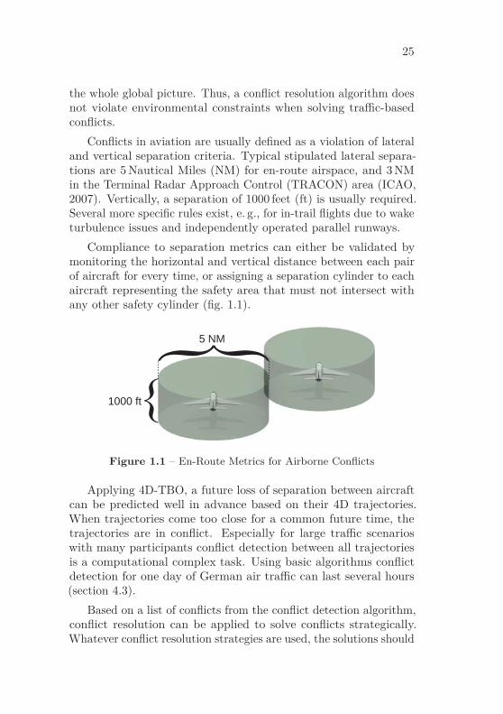
Conflicts in aviation are usually defined as a violation of lateraland vertical separation criteria. Typical stipulated lateral separa-tions are 5 Nautical Miles (NM) for en-route airspace, and 3 NMin the Terminal Radar Approach Control (TRACON) area (ICAO,2007). Vertically, a separation of 1000 feet (ft) is usually required.Several more specific rules exist, e. g., for in-trail flights due to waketurbulence issues and independently operated parallel runways.
Compliance to separation metrics can either be validated bymonitoring the horizontal and vertical distance between each pairof aircraft for every time, or assigning a separation cylinder to eachaircraft representing the safety area that must not intersect withany other safety cylinder (fig. 1.1).
{{ 5 NM
1000 ft
Figure 1.1 – En-Route Metrics for Airborne Conflicts
Applying 4D-TBO, a future loss of separation between aircraftcan be predicted well in advance based on their 4D trajectories.When trajectories come too close for a common future time, thetrajectories are in conflict. Especially for large traffic scenarioswith many participants conflict detection between all trajectoriesis a computational complex task. Using basic algorithms conflictdetection for one day of German air traffic can last several hours(section 4.3).
Based on a list of conflicts from the conflict detection algorithm,conflict resolution can be applied to solve conflicts strategically.Whatever conflict resolution strategies are used, the solutions should

26 CHAPTER 1. INTRODUCTION
be validated to really solve the conflict and not create new conflictsfurther downstream using the conflict detection algorithm again.
This work focuses on an efficient conflict detection algorithmand its impact on conflict resolution. The document is structuredas follows:
• Chapter 2 gives background information about search algo-rithms, 4D trajectories, conflict detection and conflict resolu-tion algorithms.
• Chapter 3 describes the implemented algorithm facilitatingconflict detection for an arbitrary number of dimensions.
• Chapter 4 illustrates how the generic algorithm from chapter 3is adapted, configured and optimized for conflict detection inthe aviation domain using 4 dimensions. Results from conflictdetection runs are presented for a German and a Europeantraffic sample.
• Chapter 5 focuses on conflict resolution using a trial-and-errormethod taking advantage of the high performance conflictdetection algorithm. The traffic sample covers one modifiedday of air traffic in Europe containing most direct routes fromdeparture to destination.
• Chapter 6 describes the validation of the product.
• A summary and outlook of the thesis is given in chapter 7.

Chapter 2Related Work
The chapter provides an overview about basic topics addressed bythe thesis. Section 2.1 focuses on different data structures thatare related to the tree structure of the presented conflict detectionalgorithm. An introduction on general conflict detection techniquesis given in section 2.2. Especially the conflict resolution depends onperformance limitations of aircraft. Section 2.3 provides backgrounddetails on the generation of aircraft trajectories.
Different algorithms performing conflict detection in aviationare summarized in section 2.4. Already existing conflict resolutiontechniques are described in section 2.5. Section 2.6 explains differentgeodetic Earth models and map projections in order to let aircraftfly shortest route on Earth.
2.1 Mathematics and Algorithms
This section summarizes fundamentals from mathematics and algo-rithms that are related to this work. The algorithm described isbased on N -dimensional bisection in order to reduce the problem’scomplexity.
27

28 CHAPTER 2. RELATED WORK
2.1.1 Bisection
Bisection is a method in mathematics and computer science thatrepeatedly cuts intervals into two parts. The method is used wherea complex problem can be divided into two smaller problems (Lewiset al., 1981).
A common use case is, for example, searching a number in asorted array. The number is compared to the central element of thearray. If it is bigger, the same is done within the upper interval,otherwise in the lower interval until the number is found.
The complexity of the bisection method is O(log N), with Nbeing the number of elements. Bisection can be performed using abinary tree structure.
2.1.2 Binary Tree
A binary tree is a tree data structure representing the bisectionmethod. Each node has at most two children. Depending on theuse case, the subdivision is data dependent or predefined by theinitial problem (region tree), where each node contains the dataelements corresponding to the sub-region (section 2.1.3).
2.1.3 Binary Space Partitioning Tree
Binary space partitioning (BSP) is a class of trees subdividing aspace into convex subsets recursively. The subdivision is usuallydone along hyperplanes. Famous representatives of BSP trees arequadtrees (2D) and octrees (3D). A quadtree represents a partitionof space in two dimensions. The root tile contains the entire startingregion. Each node is subdivided in four children until reaching theleaves. While quadtrees are used for segmentation of 2D-maps,octrees fulfill the identical task within 3D-space. Nodes of an octreehave 8 children generated by 3 subdividing planes, with exceptionof the leaves. Dworkin and Zeltzer (1993) propose to use a hex-treein order to represent dynamic motion of objects in a static way.The conflict detection algorithm described in chapter 3 uses anN -dimensional BSP tree.
2.1. MATHEMATICS AND ALGORITHMS 29
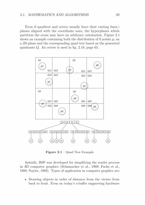
Even if quadtree and octree usually have their cutting lines/-planes aligned with the coordinate axes, the hyperplanes whichpartition the scene may have an arbitrary orientation. Figure 2.1shows an example containing both the distribution of 9 points pi ona 2D-plane and the corresponding quad tree based on the generatedquadrants Q. An octree is used in fig. 2.18, page 65.
p1
p2
p3
p4
p5
p6
p7 p8
p9
Q1 Q2
Q3 Q4
Q11 Q12
Q13 Q14Q21 Q22
Q23 Q24
Q41 Q42
Q43 Q44
Q31 Q32
Q33 Q34
Q1 Q2 Q3 Q4
Q11 Q12 Q13 Q14
p7 p1 p6p9
Q41 Q42 Q43 Q44
p2 p4
Q31 Q32 Q33 Q34Q21 Q22 Q23 Q24
p3 p8 p5
Figure 2.1 – Quad Tree Example
Initially, BSP was developed for simplifying the render processin 3D computer graphics (Schumacker et al., 1969; Fuchs et al.,1980; Naylor, 1993). Types of application in computer graphics are:
• Drawing objects in order of distance from the viewer fromback to front. Even on today’s z-buffer supporting hardware

30 CHAPTER 2. RELATED WORK
sorting is still necessary when drawing transparent objects(Kelly et al., 1994).
• Cutting complex objects into primitives easier to handle.
Other applications of BSP trees are collision detection, ray tracingand other calculations on complex spatial scenes. A special k-dimensional BSP tree is the k-d-tree.
2.1.4 k-dimensional Tree
The k-dimensional tree (k-d tree) is a BSP for organizing points ink-dimensional space described by Bentley (1975). Every non-leafnode has two children. Thus, a k-d tree splits only once per levelalong a hyperplane. Splitting a k-d tree once in every of the kdimensions creates a tree of depth k. k-d trees are not necessarilybalanced. The splitting hyperplanes are not necessarily at the centeror median point of the interval.
Figure 2.2 shows an example containing both the distributionof 9 points on a 2D-plane and the corresponding k-d tree.
Wald and Havran (2006) describe how to use k-d trees for raytracing. They provide an algorithm to build the tree in O(N log N).Instead of storing points, there are variations of the k-d tree workingon volumetric objects (Rosenberg, 1985; Houthuys, 1987).
In contrast, the algorithm proposed in chapter 3 divides up to Ndimensions in each level. A dimension is omitted for splitting only ifthe minimum tile size would be violated by the subdivision in thatdimension. Splitting hyperplanes are always aligned to axis, andalways split a dimension in the center of the interval. The simplicityof the structure allows very fast access to tree tiles utilizing smallportions of memory, only.
2.1.5 R-Tree
Another tree structure providing spatial access methods is theR-tree proposed by Guttman (1984). Manolopoulos et al. (2006)describe various types of R-trees and their applications. Key idea of

2.1. MATHEMATICS AND ALGORITHMS 31
L1
L2 L3
L4 L5
p7 p1 p2 p4
L6
p3 p8
L7
p9 L8
p5 p6
p1
p2
p3
p4
p5
p6
p7 p8
p9
L1
L2
L3
L4
L5
L6
L7
L8
Figure 2.2 – k-d Tree Example
an R-tree is to group closely spaced objects and represent them as aminimum bounding rectangle object in the next higher level of thetree. Each group has a predefined maximum number of entries. Aminimum fill is usually defined as a percentage of maximum number.Figure 2.3 shows an example containing both the distribution of 9points on a 2D-plane and the corresponding R-tree with a maximumof three entries.

32 CHAPTER 2. RELATED WORK
R1 R2
R3 R4 R5 R6
p1 p7 p3 p8 p2 p4 p5 p6 p9
p1
p2
p3
p4
p5
p6
p7 p8
p9
R1R1
R2
R4R3
R5R6
Figure 2.3 – R-Tree Example
This tree structure is especially efficient for finding the k nearestneighbor using a spatial join. A variation of the R-tree is the R*-tree storing points and volumetric objects. Beckmann et al. (1990)describe how to access points and rectangles efficiently using anR*-tree.
2.2 Conflict Detection Mechanisms
Conflict detection mechanisms are applied in many applicationfields as wire and component layout in Very-large-scale integration

2.2. CONFLICT DETECTION MECHANISMS 33
(VLSI), motion planning in robotics, solid modeling, ray tracing,Virtual Reality (VR), and many more. Common goal is usually todetect conflicts in an efficient, accurate and robust way. A goodoverview on conflict detection is provided by Mount (1997).
Identifying conflicts between two geometric objects and thecomputation of the intersection region depends strongly on the typeof objects. This section describes general techniques for collisiondetection.
2.2.1 Multiple Phases for Complex Scenarios
Scenarios for conflict detection may become very complex. Since ahigh precision conflict detection between objects often is computa-tional expensive due to high level of detail and complex metrics, adivision into two phases may be beneficial:
• The broad phase identifies potential conflicts only. This phaseusually works on low detail data (e. g., bounding boxes insteadof high detail objects) and omits as many object pairs aspossible from the second phase. A good broad phase generatesa low number of false-positives (i. e., a potential collision wasidentified, but it turns out to be a near miss) while ensuringthat it does not produce any false-negatives (i. e., existingcollisions are not identified as potential ones).
• The narrow phase performs the final collision detection withhigh accuracy. Often, the broad phase provides, in additionto the two objects, also information on where these objectsmay intersect.
If the range of detail is large, additional phases in-between may bebeneficial.
2.2.2 Discrete and Continuous Motion
Collision detection can be performed for static scenarios and sce-narios containing moving objects. The motion can be taken intoaccount in two ways:
34 CHAPTER 2. RELATED WORK
• In case of discrete motion, all objects are moved to theirpositions for a common specific time. This global time isincreased with constant or adapted steps. Collision detectionis performed on each predicted frame. The time step sizeneeds to be chosen with care. Too small time steps increasecomputational effort, while too big time steps increase theprobability of missing collisions. The optimum time step sizedepends on objects’ shapes and speeds. A chosen step size Δt
ensures that all conflicts with a minimum duration of Δt canbe found. Detection of collisions with durations less than Δt
cannot be guaranteed. The time step size for reactive real timesimulations is trivial and depends on the achievable collisionprediction rate. Even for real time simulations, a continuousmotion simulation is reasonable, because it guarantees todetect all collisions with their accurate time.
• Continuous motion avoids the discretization of time. Colli-sion detection is performed on positions depending on theadditional dimension t. Since calculation of collisions is muchmore complex without discretization of time, many methodssimulate motion discretely. However, especially for small,fine-grained objects that move fast, an adequate selection ofthe time step size is difficult.
2.2.3 Convex Polygon Intersection
The convex polygon intersection is often used in the narrow phase.Intersections between two convex polygons can be detected inlogarithmic time O(log N). An algorithm with this complexity wasproposed by Dobkin and Kirkpatrick (1983): Assuming that bothpolygons are given as a list of vertices in counterclockwise order, firstthe lowest and highest y-coordinates are determined for polygons Pand Q. Using a variant of binary search (compare section 2.1.1) thiscan be performed in O(log N). Polygons P and Q are then splitinto two convex chains PL, PR and QL, QR at lowest and highesty coordinates. Semi- infinite rays are attached to beginning andend of each chain. For right oriented chains, rays run parallel to

2.2. CONFLICT DETECTION MECHANISMS 35
the x-axis towards +∞, for left oriented towards −∞. P and Qintersect if and only if PL intersects QR and PR intersects QL.
Figure 2.4 reveals how P is split into PL and PR. Furthermoreit depicts how the median edge lines of PL and QR intersect. Ifthe intersection point is on both edges, the intersection is alreadyidentified. Otherwise, the algorithm distinguishes between an emptyregion that is untouched by both vertex chains, and the LR region,that can be reached according to the convexity assumption by bothchains. Depending on the geometry of intersection, half of at leastone vertex chain can be eliminated, marked in orange (fig. 2.5).
P
PRPL
QR
PL
Emptyregion
LR region
+
+
-
-
PL PR
x
y
Figure 2.4 – Intersection Calculation between two Convex Polygons
2.2.4 Simple Polygon Intersection
Without convexity assumption, conflict detection becomes morecomplex. First of all an algorithm is required providing a decision onthe simplicity of a given polygon. A polygon is simple if the vertexchain is not self-intersecting. A common approach to check for self-intersection is trying to triangulate the polygon. If the triangulationprocess fails, self-intersection is a possible reason. In particular, self-

36 CHAPTER 2. RELATED WORK
QR PL
Emptyregion
LR region
Emptyregion
LR region
PL
QR
+
+ +
+
-
-
-
-
x
y
Figure 2.5 – Eliminating Half of at least one Vertex Chain
intersection can be determined in O(N) using a modified version ofthe linear-time triangulation algorithm (Chazelle, 1991).
The same complexity can then be achieved for the intersectiontest of two simple polygons by merging both polygons using anarrow channel and determining self-intersection subsequently.
2.2.5 Plane Sweep Algorithms
Plane sweep is a class of algorithms detecting intersections betweenmultiple objects with usually simple geometry. Thus, a set of Nline segments can be tested for intersection in O(N log N) (Shamosand Hoey, 1976). The plane sweep method can be considered asbroad phase algorithm selecting potentially conflicting object pairs.
Plane sweep is based on simulating a left-to-right sweep on aplane using a vertical sweepline. While the sweepline goes from leftto right, a list of segments intersecting the sweepline is maintained,sorted from bottom to top by intersection point. The idea is toreduce intersection calculations to consecutive pairs in this listinstead of testing all O(N2) pairs.

2.2. CONFLICT DETECTION MECHANISMS 37
The sweepline is moved from left to right jumping from oneevent to the next. Events represent either line segment end pointsor intersections between two line segments. Events are stored in apriority queue sorted by their x-value.
Objects are usually classified as:
• Sleeping: object is not reached yet by the sweepline.
• Active: object is intersected by the sweepline.
• Dead: object is completely passed by the sweepline.
Using plane sweep all k intersections of N line segments can bereported in O((N + k) log N) time (Bentley and Ottmann, 1979).Intersections between any pair of k convex N -gons can be identifiedin O(k log k log N) time (Reichling, 1988).
Plane sweep also performs well for not too complex problemsin higher dimensions. Thus, it is possible to detect intersectionsbetween any pair of N spheres in 3D-space in O(N log2 N) time(Hopcroft et al., 1983).
2.2.6 Intersection and Range Searching
Intersection and range searching focuses on intersections betweenaxis aligned rectangles. Thus, it can be applied for rectangularobjects in the narrow phase, but also for Axes Aligned BoundingBox (AABB) broad phase calculations. According to Edelsbrunnerand Maurer (1981) two axis aligned rectangles A and B intersect if:
• A contains the left bottom point of B; or
• The left border line of A intersects with the bottom borderline of B; or
• The bottom border line of A intersects with the left borderline of B; or
• B contains the left bottom point of A.

38 CHAPTER 2. RELATED WORK
Figure 2.6 – Four Types of Intersection according to Edelsbrunnerand Maurer (1981)
Figure 2.6 depicts the four types of intersection listed above.Calculating all intersecting pairs from a set of N rectangles
can be performed in O(N log N) time for 2 dimensions (Chazelle,1988). Generalization on higher dimensions using hyper rectanglesis possible and adds an additional factor of log N in time for eachadditional dimension.
2.2.7 Bounding Volume Hierarchy
A bounding volume of a geometric object is a volume containingthe whole object. Bounding volumes simplify collision detectionespecially for complex object geometries. If two bounding volumes

2.2. CONFLICT DETECTION MECHANISMS 39
do not intersect, the corresponding objects also do not intersect.Bounding volumes with simple geometric structure allow fast detec-tion of intersections, but usually generate more false alarms becausethey cannot represent the contained object very tight. Differenttypes of bounding volumes are commonly used:
• AABBs have a simple representation and can be calculatedfast.
• Object oriented bounding volumes have a more complex rep-resentation, are more difficult to calculate, and containmentcheck is slower.
• Spherical bounding volumes allow very fast check of intersec-tion.
• k−Discrete Orientation Polytopes (dops) introduce a refine-ment of standard rectangular bounding volumes.
The idea of Bounding Volume Hierarchy (BVH) is building atree holding the object’s bounding volume in the root node. Nodesare subdivided into at least two parts by partitioning the geometricobject into at least two subsets and calculating the correspondingbounding volumes. That way, the union of bounding volumesconverges towards the shape of the geometric object with increasingdepth of the tree. The partitioning is performed until each subsetcontains one primitive only or according to a predefined abortcriterion, representing a leaf of the tree.
Conflict detection is performed on object’s root nodes first. Ifthe root bounding volumes do not intersect, the objects do notintersect. Otherwise, the children of the conflicting root nodesare examined for intersection. If the intersection test is positivebetween leaves, a conflict is very likely or even ensured, if the leaveshave the exact shape of the corresponding geometric subset.
The BVH technique is also often used for intersection tests be-tween Bézier curves. Bézier curves are frequently used in computergraphics to model smooth curves. Bézier curves allow indefinitelyscaling. Since a Bézier curve is completely contained in the convexhull of its control points (Prautzsch et al., 2002), in particular thecalculation of bounding volumes is very simple.

40 CHAPTER 2. RELATED WORK
Zachmann (1998); Klosowski et al. (1998) demonstrate how toapply BVH in VR for haptic force-feedback simulation. They inves-tigate on using different 3-dimensional bounding boxes, Klosowskiet al. concentrating on:
• 14-dops using the 6 halfspaces that define the facets of anAABB and 8 diagonal halfspaces cutting off the corners.
• 18-dops using the 6 halfspaces that define the facets of anAABB and 12 halfspaces cutting off the edges.
• 26-dops using the 6 halfspaces that define the facets of anAABB and 20 halfspaces cutting off 8 corners and 12 edges.
Bode and Hecker (2013) use BVH for conflict detection betweenairborne trajectories. They distinguish between broad and nar-row phase during the conflict detection process, where the BVHrepresents the narrow phase. The broad phase, represented bya combination of R-tree and interval tree, reduces the number ofpairwise comparisons for the narrow phase. Bode and Hecker use anolder and less performant publication of the algorithms presentedin this thesis as a baseline (see Kuenz (2011)). Current resultsprove that their approach consumes about the triple time (5 msversus 16 ms) to compare one trajectory against 30 000 others. Intheir outlook, they declare their intention to investigate on real4D-data structures for the broad phase, proposing k-d tree and BSPas candidates.
Teschner et al. (2005) propose to use BVH for collision detectionrespecting deformable objects in an adapted way. Instead of binarypartitioning, they prefer 4-ary or even 8-ary trees because of thebetter overall performance when updating or refitting the hierarchiesin case of motion. Furthermore, the hierarchy is strictly oriented onthe mesh topology of the object on generation, assuming that thistopology does not change on deformation. The article also givesdetails on techniques like stochastic collision detection, distancefields, and self collision detection. Fields of application are robotics,surgery simulation, and cloth simulation.
The approach described in this thesis does not utilize BVH. BVHis a powerful method for objects that are likely to collide. As also

2.2. CONFLICT DETECTION MECHANISMS 41
Bode and Hecker experienced, conflict detection based on BVH haslimited efficiency for sparse air traffic, necessitating a partitioning inbroad and narrow phase. Fast conflict detection avoids comparisonsbetween objects that are really far away from each other. A domesticflight in Spain cannot conflict with a domestic German flight, andthere is no need to compare any bounding boxes. Therefore, thiswork focuses on a really strong broad phase, eliminating as manycomparisons as possible in the first place. The narrow phase isrequired very rarely, and the position of a possible conflict is alreadylimited to a very small area in all dimensions. Furthermore, thecylindrical shape of objects (at least for aircraft objects) allows fastcollision detection without using BVH. Even when using complexdistance metrics like World Geodetic System 1984 (WGS84), theresults from the algorithms in use are very promising.
2.2.8 Kinetic Data Structures
Kinetic Data Structures (KDSs) are often used to model continu-ously moving objects in a geometric system, e. g., for the purposeof collision detection. According to Guibas (2001), a KDS can bespecified by
• a set of certificates defining elementary geometric relations,
• a motion plan describing the motion of objects in the nearfuture,
• events representing the violation of KDS certificates, and
• an event queue holding all events sorted by the time of certifi-cate violation.
The future time of failure for a certificate can be predicted if motionplans are available for all of its objects. An event is classifiedexternal when the combinatorial structure of the attribute changes,and internal, when the structure stays the same and the certificateneeds to be changed.
The performance of a KDS depends on four factors (Guibas,2001):
42 CHAPTER 2. RELATED WORK
• responsiveness: A KDS is responsive if the cost for repairinga failed certificate and updating the attribute computationare small. Small quantities are considered to be O(nε) in theproblem size.
• efficiency: A KDS is efficient if the number of certificatefailures is comparable to the number of external events.
• compactness: A KDS is compact if the number of certificatesis close to linear in the degrees of freedom of the movingsystem.
• locality: A KDS is local if each object participates in fewcertificates, only.
Basch et al. (1999) demonstrate how to apply KDS for collisiondetection. Instead of focusing on collision comparisons as illustratedin section 2.2.7 for BVH, Basch et al. concentrate on the free spacebetween moving objects. This free space is subdivided into cellsof a certain type. This space deforms while the objects move.The KDS proof of separation remains valid unless cells becomeself-intersecting. Desired characteristics for the cell types are
• self-collisions are easy to detect,
• tiling can adjust to the motion of the objects, and
• easy update of the tiling in case of self-collision.
Basch et al. use an external relative geodesic triangulationdefining a set of flexible shells surrounding each of the objects. Thespace between these shells is subdivided into pseudo-triangles. Oncea pseudo-triangle self-intersects as a result of moving objects, acertificate fails, either necessitating an update of the certificate orrepresenting a potential conflict.
Abam et al. (2006) illustrate how to apply KDS for collisiondetection in 3 dimensions. While most 2-dimensional approachesdecompose the free space between polygons into pseudo-triangles,a suitable decomposition for free space in 3D is less obvious. Abamet al. use guarding points around each object, assuming that the
2.2. CONFLICT DETECTION MECHANISMS 43
objects are fat. The positions of guarding points ensure that thelarger object must contain at least one guard from the smaller objectin case of collision.
The proposed solution handles events in O(log6 n) time andprocesses O(n2) events in the worst case. The authors state thattheir approach
“. . . should be seen as a proof that good bounds are pos-sible in theory–whether a simple and practical solutionexists that achieves similar worst-case bounds is stillopen.” (Abam et al., 2006)
Zachmann and Weller (2006) combined KDS with BVH to ahigh performance conflict detection for deformable objects. Whilethe pure conflict detection is performed using the BVH based onAABB and BoxTree, the KDS is used to keep the BVH up-to-dateaccording to the internal deformable object with the minimumnumber of updates.
Implementations for specialized KDS are available from theComputational Geometry Algorithms Library (CGAL) (The CGALProject, 2015). CGAL provides implementations for Delaunaytriangulation (two and three dimensions) and regular triangulation(three dimensions). Furthermore, exact and inexact operations onprimitives are supported along polynomial trajectories.
2.2.9 Sweep and Prune
Cohen et al. (1995) propose to project three dimensional AABBfrom moving 3D-objects onto the x, y, and z axes. They generatethree sorted lists, one for each dimension holding the correspondingobject intervals. By applying insertion sort, holding the lists sortedcan be performed in O(n). Furthermore, they keep track of changesin overlap status with an effort of O(n + s), s being the number ofpairwise overlaps. Whenever two objects overlap in all three lists,the corresponding polytope pair is declared active. Thus, the sweepand prune is a broad phase algorithm. The exact collision detectionroutine (i. e., the narrow phase) is called only for active polytope

44 CHAPTER 2. RELATED WORK
pairs. The motion is simulated by small time steps, assuming thatobjects are moving only slightly from frame to frame.
Coming and Staadt (2005) suggest a kinetic sweep and prunefor collision detection. Instead of simulating small time steps, theyapply a KDS to keep the interval lists sorted. An event is scheduledfor each pair of adjacent list elements to catch the crossing ofelements. Especially for linear motion, the time of crossing caneasily be predicted. That way, discrete time steps can be avoidedand time is handled continuously.
2.2.10 Broad Phase Based on Delaunay Triangu-lation
Tavares and Comba (2007) based their collision detection algorithmon a delaunay triangulation, supposed to be applied in the broadphase. While a triangle vertex represents the center of mass ofan object, the edges represent object pairs to be checked in thenarrow phase. For each frame of the animation, the triangulation isupdated. The performance results do not show benefits comparedto sweep-and-prune and brute-force bounding box methods.
2.2.11 Spatial Subdivision
When objects are small on average and they are distributed uni-formly, subdivision of their containment volume is beneficial. Typi-cal underlying structures for spatial subdivision are BSP tree (sec-tion 2.1.3), k-d Tree (section 2.1.4), and R-tree (section 2.1.5)(Samet,1990). In contrast to all aforementioned conflict detection mecha-nisms spatial subdivision can easily be used with any number ofdimensions.
2.2.12 Spatial Hashing
Spatial hashing is a special form of spatial subdivision using ahash-function mapping 3D positions to a 1D hash table index. Thehashing is performed in the broad phase, leading to a hash table

2.2. CONFLICT DETECTION MECHANISMS 45
where each index contains a small set of objects to be compared inthe narrow phase.
The idea of Teschner et al. (2003) is spatial hashing on objectsconsisting of tetrahedrons. Each primitive is mapped into a hashtable, allowing collision detection between objects and self colli-sion detection. The hash values are calculated from discretizedvertex positions (�x/l� , �y/l� , �z/l�) with l being the grid cell size.After mapping all vertices, the proposed algorithm computes allhash values that are affected by the AABB of a tetrahedron. If atetrahedron is mapped to an index containing vertices from othertetrahedrons, a penetration test is performed. Collisions betweentetrahedrons and edges are not considered. The hash function is de-fined as hash(x, y, z) = (73 856 093 ·x⊕19 349 663 ·y ⊕83 492 791 ·z)mod n, with n being the size of the hash table.
Spatial hashing does not build an explicit 3D data structure.Instead memory is used only for storing the hash table. The sizetypically depends on
• Size of the global bounding box.
• Size of objects.
• Acceptable collision risk for non-related objects being hashedon the same index.
• Inner data structure used within hash map.
Considering the scenario setup illustrated in table 4.1 onpage 125, the scenario contains 2Dx ∗ 2Dy ∗ 2Dz ∗ 2Dt cells, summingup to 239.73(∼1012) entries. Depending on the choice of the innerdata structure and the accepted overlap of hash values, a directadvantage concerning memory usage is not expectable.
Another difference between explicit spatial data structures andspatial hashing is the level of detail that needs to be taken intoaccount when inserting new objects. While the spatial hashingneeds to mark all affected grid elements, tree-structured spatialsubdivision only needs to adapt to the associated subdivision layer.Although aircraft and their occupation volume are small compared

46 CHAPTER 2. RELATED WORK
to minimum grid size, this difference especially arises when consider-ing the assigned trajectories. Thus, on insertion in a spatial hashingstructure, whole trajectories of aircraft need to be upsampled to theunderlying grid structure and mapped into the hash table. Applyingdynamic spatial subdivision, the mapping to final grid size is onlyrelevant in densely occupied areas.
2.3 4D Trajectory Prediction
When trying to detect and solve conflicts it is essential to take theproblem complexity of the application area into account. If, forexample, the motion of objects can easily be described in a closedanalytical form, an analytical solution may be beneficial. If objectsfollow complex trajectories depending on many factors as describedhere, other data representations should be preferred. Therefore, thissection describes the ways to operate an aircraft, and the predictionof an aircraft trajectory, either pre-flight or airborne.
The primary goal is to move the aircraft from the departureto the arrival airport, satisfying the very high safety standardsof air transport, in accordance with economic and environmentaldemands, and providing acceptable working conditions for the pilotcrew. While this is true for decades now, the way how to do sochanged significantly. Even though following list also represents thechronological order of employment, today all three types of controlare typically integrated in modern transport aircraft:
• The most basic way to fly a transport aircraft is by givinginstructions using the control column or side stick and thethrust lever. The pilot directly controls the aircraft.
• A more automated way of flying an aircraft is using theautopilot. The autopilot controls lateral and vertical speed,bearing, altitude and localizer/glideslope in approach mode.The pilot controls the aircraft on a higher, semi-automaticlevel.
• A Flight Management System (FMS) provides a fully auto-matic control system for flying an aircraft. The pilot enters

2.3. 4D TRAJECTORY PREDICTION 47
whole routes into the FMS. The system predicts a trajectoryfrom departure to destination and automatically guides theaircraft along this route. The pilot manages the aircraft. Thepilot still may use the control systems above, however thisdecreases predictability and typically efficiency of flight. Thelower level systems are the safety net for the FMS.
Figure 2.7 shows the cockpit from the former research aircraftAdvanced Technologies Testing Aircraft System (ATTAS) oper-ated by Deutsches Zentrum fuer Luft- und Raumfahrt (GermanAerospace Center) (DLR) providing all aforementioned ways ofcontrolling an aircraft. The ATTAS is a Vereinigte FlugtechnischeWerke (VFW) 614 twin engine jet transport aircraft modified withworldwide unique equipment for research purpose (fig. 2.8). ATTASwas recently retired after 26 years in service. Its direct successoris Advanced Technology Research Aircraft (ATRA), a modifiedAirbus A320-232.
Figure 2.7 – ATTAS Cockpit allowing 3 Ways of Flying
ATTAS is equipped with one of world’s most advanced FMS.The Advanced Flight Management System (AFMS) was developedby the Institute of Flight Guidance at DLR Braunschweig. Variousflight trials with ATTAS and also first trials with ATRA proved

48 CHAPTER 2. RELATED WORK
Figure 2.8 – DLR’s former Research Aircraft ATTAS
high accuracy and flexibility of the AFMS (Korn and Kuenz, 2006;Kuenz et al., 2007).
Using an FMS for automatic flight execution does not onlyreduce pilot’s workload but is also the on-board technical enablerfor TBO.
2.3.1 The Advanced Flight Management System
This section holds a description of DLR’s AFMS being a good rep-resentative for a modern FMS. The initial version of the AFMS wasstarted in early 1990s (Adam and Kohrs, 1992; Kohrs, 1992; Czerl-itzki, 1994; Czerlitzki and Kohrs, 1994) and since then continuouslyimproved.
By means of strategic trajectory planning and a correspondingguidance module the AFMS allows planning of highly accurate 4D-trajectories and following them with little deviations autonomously.
Figure 2.9 shows the in- and output data of the AFMS. Gener-ation of 4D-trajectories is performed based on a list of waypointsdescribing the route from departure (or actual position when alreadyairborne) to the destination, altitude, speed and time constraints,aircraft’s performance data and an accurate weather forecast. Theweather forecast for flight trials is provided by Germany’s national

2.3. 4D TRAJECTORY PREDICTION 49
List of Waypoints
Altitude, Speed and Time
Constraints
Aircraft Model
Weather Forecast
Descent Parameter
AFMS Cockpit
ATTASReal Weather
Figure 2.9 – In- and Outputs of AFMS
meteorological service Deutscher Wetterdienst (DWD). Using thedescent parameters given by the pilot the AFMS allows predicting:
• Low Drag Low Power (LDLP) approaches with selected in-tercept altitude and level length. LDLP tries to use cleanconfiguration as long as possible. Besides a significantly highernoise emission, extracting slats, flaps and gear increases dragand thus reduces flight’s efficiency. However, the LDLP inter-cepts the final glideslope in level flight in order to allow lateadjustments for the final descent.
• Continuous Descent Approach (CDA) with selected interceptaltitude. The CDA also makes use of low drag configura-tions. Furthermore, CDA avoids the final level at glideslopeintercept. Therefore, the aircraft flies higher and thus moreefficient. Noise pressure level immissions on the ground arereciprocally proportional to the altitude, doubling the altitudereduces noise pressure level by 50 % (Deutsches Institut fürNormierung, 1999).
• Segmented Continuous Descent Approach (SCDA) with se-lected start of steep descent and intercept altitude. The steep
50 CHAPTER 2. RELATED WORK
descent profile is produced by an early configuration in highaltitudes. The steep descent part is flown with flaps andgear out. Drag is increased for this procedure, and thus alsofuel burn. However, depending on aircraft type, the noiseinfluence of the higher altitude of the profile can outweigh theincreased noise emissions due to configuration.
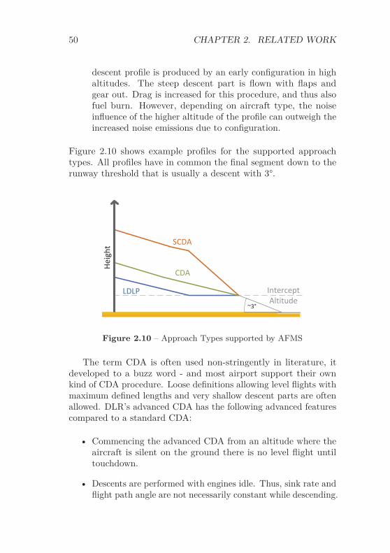
Figure 2.10 shows example profiles for the supported approachtypes. All profiles have in common the final segment down to therunway threshold that is usually a descent with 3°.
Height
InterceptAltitude
LDLP
CDA
SCDA
~3°
Figure 2.10 – Approach Types supported by AFMS
The term CDA is often used non-stringently in literature, itdeveloped to a buzz word - and most airport support their ownkind of CDA procedure. Loose definitions allowing level flights withmaximum defined lengths and very shallow descent parts are oftenallowed. DLR’s advanced CDA has the following advanced featurescompared to a standard CDA:
• Commencing the advanced CDA from an altitude where theaircraft is silent on the ground there is no level flight untiltouchdown.
• Descents are performed with engines idle. Thus, sink rate andflight path angle are not necessarily constant while descending.

2.3. 4D TRAJECTORY PREDICTION 51
Idle thrust does not only reduce noise emissions of the enginesbut also reduces noise immissions on the ground and fuelconsumption due to higher and therefore more economicalflight profiles.
• The vertical profile can be specified independently of thelateral path. This enables the implementation of specialprocedures like curved approaches.
One main task when calculating a 4D-trajectory performing a CDAis to predict an appropriate position for the Top Of Descent (TOD).First, the AFMS calculates the glideslope intercept point by meansof glideslope angle, intercept altitude and runway threshold positionand elevation. The AFMS calculates the TOD by stepping backwardfrom the glideslope intercept point (see fig. 2.11), implying an idledescent to the glideslope intercept.
Glideslope, ~3°
Idle DescentLevel Flight TOD
Glideslope Intercept
Figure 2.11 – Calculating the TOD
The foreseen airspeeds depend on phase of flight and type ofaircraft. Optimum speeds for different flight phases and all otherrelevant information about aircraft are published for most trans-port aircraft by the European Organisation for the Safety of AirNavigation (Eurocontrol) in the Base of Aircraft DAta (BADA),current version in use is 3.9 Eurocontrol (2011).
Once having generated a 4D-trajectory the AFMS providesguidance commands to fly along the calculated trajectory. A 4D-tra-jectory consists of a lateral route with altitude and time informationfor every waypoint. If an appropriate connection to the autopilot isavailable these commands are directly forwarded to the aircraft thatwill automatically follow the trajectory. If such a connection is notavailable the guidance commands can be displayed as instructions

52 CHAPTER 2. RELATED WORK
to be carried out by the pilot. The AFMS guidance commandscontrol the aircraft in all 4 dimensions (lateral, vertical and time).
0 4 8 12 16 20 24 28 32
0 4 8 12 16 20 24 28 32Duration : 00:09:35Used Fuel : 329 kg
Distance along Route [NM]
kts
CAS:
Altitude:
140160180200220240
ft
500100015002000250030003500400045005000550060006500700075008000
IdleDescent
Descent Deceleration
Descent Deceleration 250 190 kts DescentDeceleration190 170 kts
DescentDeceleration
DescentDeceleration160 133 kts
Flaps 1Flaps 2
Flaps FullGear Down1800ft AGL
WAYP0
DIRAL
ALESI
VE028
LERDI
RW26
Figure 2.12 – CDA Trajectory for Airbus A330-300
For a precise prediction and guidance along 4D-trajectoriesthe AFMS has also to consider the aircraft’s configuration. Thehigher drag and lift coefficients of extended flaps otherwise leadsto deviations which might not be accepted in a 4D TBO trafficmanagement, as described by de Muynck et al. (2011).
Figure 2.12 depicts an example of an advanced CDA calculatedby the AFMS for the Airbus A330-300. Usually, a flight is subdi-vided into five phases: Departure (Dep), Climb (Clb), Cruise (Crs),Descent (Dsc) and Arrival (Arr). The example starts in cruiseflight.
The TOD is in Flight Level (FL) 80 where the aircraft is in cleanconfiguration. The descent starts idle with a constant CalibratedAir Speed (CAS) of 250 knots (kts). This is followed by an energysharing phase where the aircraft both descents and decelerates. Theglideslope is intercepted at 3000 ft with 170 kts, flaps just coming

2.3. 4D TRAJECTORY PREDICTION 53
out to position 2. At 1800 ft above ground level the aircraft isconfigured for landing (flaps full, gear down). Flying the standardglideslope approach the aircraft will need thrust to hold the landingspeed on the very last part before landing. Deviations may occurduring the execution of an advanced CDA due to:
• Insufficient or imprecise aircraft performance data.
• Jitter in the configuration points.
• Bad weather forecast.
• . . .
When forced to deviate from the predicted trajectory because ofunforeseen influence described above, the AFMS guidance function-ality tries to hold the time deviation at minimum and in exchangeaccumulate the altitude error. The altitude error is compensatedwhen intercepting the glideslope. This type of readjustment dependson whether the aircraft is too high or too low.
Being in time and having a positive altitude error (aircraft istoo high) means that the aircraft has too much energy left. Sincethe engines are idle in descent there is no way out with the thrust.Therefore, the AFMS reacts by increasing the drag. If the AFMSdetects a positive altitude error when intercepting the glideslope itbrings forward dynamically the configuration times for flaps andgear. A negative altitude error (aircraft is too low) implies a lackof kinetic energy. An early reaction in form of setting higher thrustshould be avoided because:
• Slow response times of jet engines make a closed loop controldifficult.
• Even small changes of the engine speed are felt disturbing bythe passengers.
A negative altitude error is corrected by insertion of a less steepsegment. Only in extreme cases this segment will be a level segment.In order to get rid of the missing energy, the AFMS brings forwardthe point of leaving idle thrust. Thus, there is no new phase of

54 CHAPTER 2. RELATED WORK
closed loop low power control but a small extension of the thrustphase just before landing.
Figure 2.13 and fig. 2.14 are noise footprints for an AirbusA320 approach to Frankfurt via Gedern. The trajectories werecalculated by the AFMS and fed into the DLR noise calculationtool SIMUL (Boguhn, 2007). The noise areas start with a darkblue for >55 dB(A) and increase in steps of 5 dB(A). The differencebetween fig. 2.13 and fig. 2.14 illustrates the noise benefit achievableby selecting the advanced CDA descent in favor of LDLP.
Figure 2.13 – Noise Footprint of LDLP
The AFMS prediction and guidance capabilities have been vali-dated in several simulation runs using the A330-300 Full FlightSimulator formerly operated by the Zentrum für FlugsimulationBerlin (ZFB) and flight trials with DLR’s test aircraft ATTAS andATRA.
Both the simulations and real flight trials were performed start-ing in FL70-FL110 with enough way left to touchdown allowing

2.3. 4D TRAJECTORY PREDICTION 55
Figure 2.14 – Noise Footprint of CDA
prediction of advanced CDA and LDLP approaches. The ATTASand ATRA flights were arranged at the base airport Braunschweigprincipally using the runway 26. The destination airport for theA330 simulations was Munich.
Figure 2.15 displays a typical result of an advanced CDA ap-proach with ATTAS. The figure depicts with a red line the occurredaltitude error with a maximum of 70 ft, the airspeeds, the times offlaps and gear transitions and the altitude profile. Typical precisionfor more than 100 approaches was a maximum of ±150 ft altitudeerror and ±5 s time deviation at the touchdown point.
The figure also shows that the altitude error peaks are at thetransitions from one flight path angle to the next, e. g., at the TODand the glideslope intercept point. This behavior is reasoned by thefact that the AFMS does not calculate flight path angle transitionsand therefore they are not part of the trajectory. Hence, the altitudeerror calculation by building the difference between actual altitudeand trajectory tends to be bigger than the real altitude error.

56 CHAPTER 2. RELATED WORK
7000
Altitude:
ft
500
15001000
2000250030003500400045005000550060006500
22 24 26 28 30 32 34 36 38 40
Alt Error:
CAS:
ft
kts
VE028
LERDI
RW26
ALESI
22 24 26 28 30 32 34 36 38 40
22 24 26 28 30 32 34 36 38 40200190180170160150140
500
50100150
150100
DIRBO
Figure 2.15 – CDA flown by ATTAS
Two flight trials have been untypical with a time precision ofrather bad 10 seconds. Investigations revealed that an impreciseweather forecast reasoned the unusual time deviation. On oneoccasion, the Harz mountains created a constant downdraft intheir lee, where Braunschweig is situated, but the weather forecastfile only contained information about the horizontal wind and notabout vertical wind components. On the other occasion, a minijet stream was encountered between 5000 ft and 10 000 ft, but thewind was only forecasted at these two altitudes and around, notin-between. Thus the jet stream was not detectable in the winddata and not taken into account when predicting the trajectory.Finally, considering the imprecise weather forecast, a time deviationof 10 seconds is not bad at all for more than 30 NM of flight.
The main driving factor for the A330 simulations was to provethe usability of the AFMS for any aircraft listed in the BADAfolder (currently 295 aircraft) and not ATTAS only. The resultsin fig. 2.16 prove high quality of the AFMS prediction as well as asuitable BADA modeling. Top down, the figure depicts the time
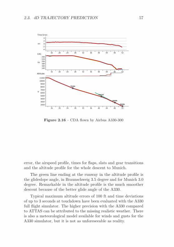
2.3. 4D TRAJECTORY PREDICTION 57
11000
Altitude:
ft
Time Error:
CAS:
sec
kts
240220200180160140
024
42
1000090008000700060005000400030002000
16 20 24 28 32 36 40 44 48 52
16 20 24 28 32 36 40 44 48 52
16 20 24 28 32 36 40 44 48 52
TEGBA
MAGAT
OM08L
RW08L
Figure 2.16 – CDA flown by Airbus A330-300
error, the airspeed profile, times for flaps, slats and gear transitionsand the altitude profile for the whole descent to Munich.
The green line ending at the runway in the altitude profile isthe glideslope angle, in Braunschweig 3.5 degree and for Munich 3.0degree. Remarkable in the altitude profile is the much smootherdescent because of the better glide angle of the A330.
Typical maximum altitude errors of 100 ft and time deviationsof up to 3 seconds at touchdown have been evaluated with the A330full flight simulator. The higher precision with the A330 comparedto ATTAS can be attributed to the missing realistic weather. Thereis also a meteorological model available for winds and gusts for theA330 simulator, but it is not as unforeseeable as reality.

58 CHAPTER 2. RELATED WORK
2.4 Conflict Detection in Aviation
Several algorithms already exist performing conflict detection inaviation. Nowadays, a conflict in aviation based on radar and/orAutomatic Dependent Surveillance-Broadcast (ADS-B) positiondata usually exists if lateral distance in latitude/longitude planeis lower than 5 NM and the vertical distance is below 1000 ft. Inthe vicinity of airports in approach and departure phase, a reducedseparation is often used depending on wake categories of bothpreceding and succeeding aircraft. Bigger aircraft produce strongerwake turbulence while smaller aircraft are more sensitive to waketurbulence areas. The International Civil Aviation Organization(ICAO) defines separations collected in table 2.1 (ICAO, 2007),based on following categories:
• Heavy (H): All aircraft types with 136 000 kg or more maxi-mum take-off weight.
• Medium (M): All aircraft types with less than 136 000 kg, butmore than 7000 kg maximum take-off weight.
• Light (L): All aircraft types with 7000 kg or less maximumtake-off weight.
Table 2.1 – Separation in [NM] Depending on Wake Categories
Preceding aircraftHeavy Medium Light
Succeeding aircraftHeavy 4 3 3Medium 5 3 3Light 6 5 3
Although the Airbus A380 is classified as heavy it produces sig-nificantly more wake turbulence than all other heavy classifiedaircraft. Therefore, the ICAO advises 6 NM distance to succeedingheavy, 7 NM distance to succeeding medium, and 8 NM distance tosucceeding light aircraft (ICAO, 2008).

2.4. CONFLICT DETECTION IN AVIATION 59
In addition, special separation requirements exist for paralleland nearly parallel runways. According to ICAO (2004b), two majormodes of operation are distinguished for arrivals:
• For independent parallel approaches, radar separation minimaare not prescribed for aircraft on extended runway center lines.
• For dependent parallel runways, radar separation minima areprescribed for aircraft on extended runway center lines.
According to ICAO (2004a), the minimum separation for de-pendent approach operations between runway center lines is 915 m;independent operations are recommended with at least 1035 m sep-aration. If the airport’s Secondary Surveillance Radar (SSR) doesnot provide:
• a minimum azimuth accuracy of 0.06 degrees; or
• an update period of 2.5 seconds or below; or
• a high resolution display featuring position prediction anddeviation alert;
a larger distance of 1310 m or even 1525 m is necessary for inde-pendent parallel approach operations, depending on whether theaircraft operation would be adversely affected. However, at least aminimum azimuth accuracy of 0.3 degrees or better and an updateperiod of 5 seconds or less is required for independent approachoperations.
Dependent runway approaches foresee a 3 NM radar separa-tion for flights approaching on the same runway and 2 NM radarseparation for aircraft landing on adjacent runways.
ICAO (2004b) also defines dependent and independent parallelrunway operations for departures and mixed mode.
2.4.1 Conflict Situations in Aviation
Conflict detection is necessary in different situations with differenttime horizons. This section gives a summary on conflicts in aviation,starting with the longest planning horizon.

60 CHAPTER 2. RELATED WORK
2.4.1.1 Sector Load and Flow Control Conflicts
Every aircraft flying according to IFR in Europe needs to file aflight plan and feed it into the Central Flow Management Unit(CFMU). The flight plan contains, amongst others:
• Estimated time of departure and arrival.
• Cruise speed.
• Requested flight route.
• Cruise flight level.
• Departure and arrival airport.
• Alternate airport.
• Type and callsign of aircraft, wake category.
• Number of persons on board.
Based on the flight plan, the CFMU (operated by Eurocontrol)assigns slots at departure and arrival airports. The CFMU validatesthat all sectors used by the requesting aircraft are still below theirmaximum load limit. The load factor of sectors is not calculated onsingle aircraft events, but estimated on traffic flows. Time horizonfor CFMU planning goes from 6 days to one hour before departure.
2.4.1.2 Trajectory Based Conflicts
Modern ATM concepts are often based on TBO. Every aircraftflies according to a 4D trajectory that is conflict free from all othertrajectories. Furthermore, additional information can be takeninto account as weather phenomena, restricted areas and otherconstraints. TBO can be performed with several time horizons:
• Strategical: Several months before departure, airline opera-tion centers need to have rough estimations of departure andarrival times, e. g., in order to sell tickets. Typically, accuracyof these predicted times is rather low because they are based

2.4. CONFLICT DETECTION IN AVIATION 61
on vague weather forecasts. However, even if the predicted tra-jectories differ from the really flown ones, a general feasibilityproof based on individual flights can be performed.
• Pre-tactical: Coming closer to the departure time, trajecto-ries can be updated with more accurate information. Chang-ing trajectories necessitates new conflict detection and resolu-tion.
• Tactical: When aircraft cannot comply with their assignedtrajectories, new trajectories need to be predicted that areconflict-free from the surrounding traffic and other constraints.
2.4.1.3 Medium-Term Conflict Detection
Medium Term Conflict Detection (MTCD) recognizes conflicts ofan aircraft usually with a time horizon of 20 minutes ahead atmaximum. This conflict detection can be based on different data,e. g., on trajectories using TBO, aircraft intend data broadcastedvia ADS-B, or extrapolation of current flight data.
2.4.1.4 Short-Term Conflict Alert
Short Term Conflict Alert (STCA) is usually used as an Air TrafficController (ATCo) support tool with a prediction horizon of 2minutes. STCA is integrated as a safety net; its presence is ignoredwhen calculating airspace capacity. The conflict detection is usuallybased on extrapolating current aircraft state data.
2.4.1.5 Airborne Collision Avoidance System
The Airborne Collision Avoidance System (ACAS) was introducedin order to reduce (near) midair collisions (Eurocontrol, 2012).ACAS is the last safety net on the air side. The conflict detectionis based on SSR transponder signals; non transponding aircraft arenot detected. ACAS works on small time scale. The maximumgeneration time of a traffic advisory is 48 seconds before reachingthe Closest Point of Approach (CPA). With a maximum generation

62 CHAPTER 2. RELATED WORK
of 35 seconds, ACAS issues a resolution advisory. According to(ICAO, 2002), ACAS I supports see and avoid but does not provideresolution advisories. Resolution advisories are always vertical intoday’s dominant version ACAS II, and coordinated with otherACAS II equipped aircraft via a selective mode S link, so that twoaircraft choose complementary maneuvers.
2.4.2 Trajectory-Based Conflict Detection
Conflict detection on a set of N aircraft trajectories can easily beperformed by brute-force conflict detection between every possiblepair of two trajectories. This results in N(N −1)/2 comparisons andthus a complexity of O(N2). A conflict between two trajectoriest1, t2 can be detected by segment and point comparisons of the twotrajectories (Schwoch, 2008).
The segment based method compares every segment of t1 withevery segment of t2. If both segments described by great circlesubsets intersect, a collision is detected. However, this approachdoes not detect parallel conflicting trajectories.
Therefore, the point based method compares each trajectorypoint of t1 with the time-corresponding point of t2, and the otherway round. If the distance is below the mandatory separationdistance, a conflict is detected.
If trajectory points are too sparse, new interpolated trajectorypoints are added in order to catch all conflicts. This procedure isused as the baseline conflict detection algorithm for performancetests in chapter 4. As the algorithm’s complexity indicates thismethod is not reasonable for large scenarios with many trajectories.
An advanced baseline can be defined by adding an optimization:trajectories not having a common time frame (i. e., t1 arrives beforet2’s departure, or t1 departs after t2’s arrival) are early omitted sincethey do not conflict. This method is used as advanced referencein chapter 4. The performance benefit of the optimized baselinealgorithm is significant.
Further optimization following the same basic idea was per-formed within the Programme for Harmonised Air Traffic Manage-

2.4. CONFLICT DETECTION IN AVIATION 63
ment Research in Eurocontrol (PHARE). Kremer et al. (1999)proposed a method of performance increase by means of coarsefilters. Coarse filtering reduces number of trajectory pairs underinvestigation for a final conflict check. If aircraft do not have over-lapping flight levels, the corresponding pairs can be omitted forconflict detection. Furthermore, Kremer proposed to cut flightsinto the parts departure, en-route, and descent. For each part, thebounding boxes can be checked for intersection with the potentialconflict partner’s bounding boxes to reduce number of final conflictprobes.
2.4.3 Subdivision of Airspace
Koeners and de Vries (2008) described an approach on how tosubdivide a given airspace in three dimensions (latitude, longitudeand time) to reduce the effort of conflict detection. A static grid isfilled by trajectories, grid cells are either marked as occupied or free(fig. 2.17). Cells occupied by only one trajectory are colored blue fortrajectory 1 and green for trajectory 2, while cells occupied by bothtrajectories are colored red. Koeners and de Vries propose a cellsize being half of the separation size. When storing routes in thegrid, a cell buffering technique copies data also to all neighboringcells (Jardin, 2005). Since the subdivision is static this method isonly reasonable for strongly limited geographical areas, e. g., theterminal maneuvering area of an airport.
An octree subdividing latitude, longitude and altitude is usedby Hildum and Smith (2004); Smith (2008). Subdivision is appliedeach time an octant contains a conflict. The octree is stored usinga linear octree structure as described by Gargantini (1982). Theidea of a linear octree is a linear access on octants by means ofa key derived from the latitude, longitude and altitude position.This allows access on every octant organized in a binary tree inO(log N) time. Each octant then stores a list of intersecting objectswith the corresponding intersection times. Figure 2.18 shows anexample of a conflict situation. The proposed algorithm also checksneighbor-octants in order to detect every conflict.

64 CHAPTER 2. RELATED WORK
Longitude
Tim
e
Figure 2.17 – Example Grid with Conflict according to Koenersand de Vries (2008)
This approach is especially beneficial if time extension of thescenario is small, and separation is guaranteed laterally or vertically.The described method is not efficient for areas majorly ensuringseparation by time, e. g., an octant containing the threshold of anarrival runway.
Jardin (2003) uses a static 3D-grid subdividing latitude, longi-tude and time. He applies a grid spacing of 5 NM and 30 secondsin time, resulting in ∼16 MiB of memory necessary for Continen-tal United States per flight level. Each grid cell holds a singlebinary value indicating if the cell is occupied by other aircraft orweather. An explicit conflict list is not generated by the algorithmsince Jardin performs direct conflict solution when a new trajec-tory conflicts with already occupied cells on insertion. Of course,neighboring cells also need to be taken into account.
Jen Chiang et al. (1997) proposed a static 3D-geometric subdivi-sion with minimum requested separation size. Conflicts are detectedby searching multiple aircraft in one tile and the 26 surroundingneighbors. This approach is fast since most neighbor tiles are emptyin practice. However, the tests need to be performed for severaldiscrete times with time offset Δt. Section 3.3.1 describes a differentmethod for handling neighborhoods.

2.4. CONFLICT DETECTION IN AVIATION 65
V3
V1
V2
V3V3
Figure 2.18 – Conflict in Octree between V1 and V2 according toHildum and Smith (2004)
2.4.4 Conflict Detection Considering Uncertain-ty
Amongst others, Erzberger investigated the idea of respecting tra-jectory uncertainties in conflict detection (Erzberger et al., 1997).Claiming at least 10 minutes ahead time for conflict detection, theoptimum time is a trade-off between efficiency and certainty. Theearlier a resolution maneuver is initiated, the more efficient it is.However, the more look ahead time is applied on trajectories, themore uncertainty is integrated in the conflict decision.
The conflict detection functionality is based on trajectoriesand statistical model of prediction errors, represented as ellipsoidsin three-dimensional space (fig. 2.19). In order to limit conflictdetection trials, Erzberger et al. propose three methods:

66 CHAPTER 2. RELATED WORK
Predicted Time
Predicted Time
Path Cross Angle
Prediction Error Ellipse
Minimum Predicted Separation
Predicted Trajectories
Figure 2.19 – Trajectory Prediction Error Ellipses according toErzberger et al. (1997)
• Trajectory pair pruning omits conflict detection if trajectoriesare spatially exclusive in either altitude or horizontal position.Therefore, it is checked if the trajectories fly in separated flightlevels and if their lateral bounding boxes intersect. That way,60 % to 80 % of all possible trajectory pairs are pruned.
• Separation computations are minimized. For example, lateralcalculations are avoided if aircraft are already separated ver-tically. Lateral cross-distances are calculated only if x- andy-distance are both below laterally required separation.
• Time skipping avoids conflict detection on trajectory segmentsthat are already ensured to have no conflict. Thus, if twotrajectories have a big distance at one test time τ , theirdistance is assumed to not converge faster towards zero than10 000 ft min−1 vertically and 0.33 NM s−1 (about 2 Mach atstandard sea level conditions) laterally. Therefore, if two

2.5. CONFLICT RESOLUTION IN AVIATION 67
aircraft have a distance of 200 NM at a given time τ , it is notnecessary to test them again before τ + 10 minutes.
The combination of the above described methods leads to a conflictdetection time of 10 seconds for up to 800 trajectories and a predic-tion horizon of 30 minutes running on the scalable multi-workstationarchitecture of Center-TRACON Automation System (CTAS).
In contrast to Erzberger’s proposal the conflict detection algo-rithm described in this work has no direct support for uncertaintymanagement for several reasons:
• Trajectory prediction and execution accuracy has increasedin the last decades, compare section 2.3.1.
• A prediction horizon of 30 minutes is not enough in a TBOenvironment handling gate-to-gate traffic. An uncertaintyforecast for flights lasting several hours is hard to predict, ifpossible at all, with an acceptable accuracy.
• This approach handles whole trajectories. Thus, it coversalso the bottlenecks of today’s airspace, which are usually therunways. Aircraft are staggered densely on runways both forarrivals and departures. Allowed deviations from their fore-seen trajectories is only few seconds in arrival and departurephase. Including uncertainties that accumulate during theflight to the arrival phase decreases runway’s throughput toan unacceptable level.
2.5 Conflict Resolution in Aviation
In general there are three types of conflict resolution in aviation asdepicted in fig. 2.20:
• Lateral conflict resolution avoids a predicted conflict by alateral detour.
• Vertical conflict resolution lets one aircraft sink below or climbabove the conflict partner.
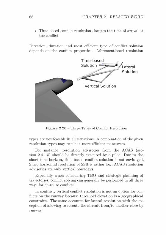
68 CHAPTER 2. RELATED WORK
• Time-based conflict resolution changes the time of arrival atthe conflict.
Direction, duration and most efficient type of conflict solutiondepends on the conflict properties. Aforementioned resolution
Figure 2.20 – Three Types of Conflict Resolution
types are not feasible in all situations. A combination of the givenresolution types may result in more efficient maneuvers.
For instance, resolution advisories from the ACAS (sec-tion 2.4.1.5) should be directly executed by a pilot. Due to theshort time horizon, time-based conflict solution is not envisaged.Since horizontal resolution of SSR is rather low, ACAS resolutionadvisories are only vertical nowadays.
Especially when considering TBO and strategic planning oftrajectories, conflict solving can generally be performed in all threeways for en-route conflicts.
In contrast, vertical conflict resolution is not an option for con-flicts on the runway because threshold elevation is a geographicalconstraint. The same accounts for lateral resolution with the ex-ception of allowing to reroute the aircraft from/to another close-byrunway.

2.5. CONFLICT RESOLUTION IN AVIATION 69
Several publications already handle conflict resolution. Thefollowing sections give an extract.
2.5.1 Conflict Resolution using Trial-and-Error
Erzberger et al. (2010) propose to not only search for one solutionsolving the conflict under investigation but continue the search andafterwards select the best from several solutions. A major factorfor a good solution is a small introduced time delay. Since conflictresolution is complex, Erzberger et al. distinguish several casesfor lateral (fig. 2.21), vertical (fig. 2.22) and time-based (fig. 2.23)solutions.
Direct-To
Left/Right Path Stretch
Analytical Turn
Left/Right Route Offset
Figure 2.21 – HorizontalResolution according to Erz-berger et al. (2010)
Step Altitude Climb/Descent
Temporary Altitude, Climb
Temporary Altitude, Descent
Figure 2.22 – Vertical Reso-lution according to Erzbergeret al. (2010)
Some of the resolution types are not applicable in any circum-stance. For instance, the lateral direct-to maneuver depends on anexisting dogleg that can be bypassed directly to a waypoint furtherdownstream. Doglegs are commonly used today but should not bestandard in envisaged TBO. In exchange, if a direct-to is possible itis usually even more efficient than the unresolved situation before.
According to Erzberger et al., the path stretching has the bestsuccess rate among the horizontal resolution types. The additionalwaypoint is put on an ellipse with the aircraft’s position as onefocus and the return point as second focus. The radii depend onthe specified delay.

70 CHAPTER 2. RELATED WORK
Mach
Time
Time
True Airspeed
Top of Descent
Figure 2.23 – Time-BasedResolution according to Erz-berger et al. (2010)
Summarizing, Erzberger et al. create ∼128 potential solutions(2 direct-to, ∼16 vertical, 6 analytical turn, 4 route offset, ∼80path stretch, and ∼20 speed). Based on these, he generates ∼128trial trajectories with a trajectory predictor and probes them in theconflict detector. From up to 15 solutions, he chooses the one thatfits best according to predefined metrics.
2.5.2 Conflict Resolution using Genetic Algo-rithm
Durand et al. (1996) propose to solve conflicts globally with geneticalgorithms. Starting with a population of conflicting trajectories,three basic operators are used to influence conflicts: selection,mutation and crossover. A fitness function is defined, definingthe desired properties of the population, e. g., having no conflictsand being cost efficient. The selection operator picks suitableindividuals from the population to breed a new generation. Themutation operators ensure genetic diversity by changing one or morevalues from single individuals. The crossover operator generateschildren based on more than one parent individual. The processiterates as long as fitness improves. Problems of genetic algorithmsare:

2.5. CONFLICT RESOLUTION IN AVIATION 71
• Quality of the overall process strongly depends on the qual-ity of the fitness function. Defining a good fitness functionsometimes is a difficult task. If the fitness function is com-plex, frequent calls destroy the overall performance. Fitnessfunctions should be continuous instead of false/true in orderto give hints for convergence direction.
• Genetic algorithms scale badly with complexity. Large popu-lations with many parameters span a large search space.
• Genetic algorithms tend to converge to local optima insteadof finding a global optimum. This behavior can be avoidedby changing the fitness function appropriately.
• It is difficult to estimate convergence behavior and time to so-lution. Certification of genetic algorithms is (at least) difficultin aviation.
2.5.3 Conflict Resolution based on PotentialFields
Another approach of solving conflicts is based on potential fields’theory (Kelly and Eby, 2000; Roussos et al., 2008). The basic ideais to use an electrostatic modeling of the problem where aircraftare handled as electrons with negative charge. Since same chargespush away each other, conflict avoidance is directly integrated inthe model. Destinations have a positive load which attracts aircraft.Aircraft are moving towards their destination while being influencedfrom the resulting electric field. Thus, aircraft/ electrons beinginstantiated at their departure fly a most likely conflict free routetowards their destination.
Calculation of complex global situations is very demanding andtime consuming using potential fields. Therefore, this kind of con-flict resolution is mostly used on local conflict situations. A bigproblem is constraining the algorithm in order to get flyable trajec-tories respecting the performance and maneuverability limitationsof aircraft and constraints from ATM.

72 CHAPTER 2. RELATED WORK
2.5.4 Conflict Resolution based on Light Propa-gation
Dougui et al. (2010) propose an algorithm based on the differentrefractions of light. Refraction indices are assigned according tothe congestion of airspace. Optimal trajectories are then found bycalculating the shortest light path between two points respectingthe local metrics built, e. g., from refraction indices and aircraftprotection zones. Calculation times are reduced by limiting thesearch space using a branch-and-bound method.
The proposed algorithm runs in (2D+time) and usually comesup with a flyable conflict free trajectory.
2.5.5 Conflict Avoidance in Crowd Simulation
Crowd simulation is often used in computer graphics and movieproductions when the movement and behavior of a large amount ofobjects and characters shall be simulated. The individual entitiesbehave according to assigned rules and thus interact with their en-vironment, e. g., by avoiding conflicts with other entities. Althoughcrowd simulation is often used to simulate human behavior in a3-dimensional system, the same mechanisms can easily be adaptedto a 4-dimensional system simulating aircraft traffic.
Foudil et al. (2009) perform crowd simulation in a discretizedcoordinate system modeled as a grid of cells. The path of an objectis generated using the A∗ algorithm (Hart et al., 1968), each objectoccupying one cell at each time. The predicted path is collision freefrom static objects. Conflicts with other entities are classified inToward (head-to-head), Away (overtake situation) and Glancing(side-on). Conflict avoidance is then performed on human lifeexperience, e. g., by taking the smallest deviation for the Towardcase and performing a slow down to avoid an Away collision.
Unfortunately, the proposed fallback procedure to stop walkingwhen no solution can be found is not directly transferable on aircraft,being strongly limited by deceleration gradient and minimum airspeed. Especially queuing at saturated arrival runways requiresother techniques, preferably with a larger look ahead time.

2.6. GEODETIC EARTH SYSTEMS 73
Golas et al. (2013) propose a hybrid approach of local collisionavoidance in the vicinity of crowd entities and approximate, long-range collision avoidance. The long term look ahead is based on anextrapolation of the known path. In order to avoid wrong decisionsbased on approximated data, the look ahead time is restricted.
Even though the approach of Golas et al. has a higher poten-tial to draw near the overall optimum than a pure local collisionavoidance, a centralized global system seems more suitable to findthe most efficient solution than a distributed crowd simulation witheach entity having a very restricted view.
2.5.6 Extended Flight Rules
The Extended Flight Rules (EFR) do not provide an algorithmsolving conflicts but a method to identify for a conflict situationwhich aircraft has right of way (Duong et al., 1996). The priorityassignment considers maneuverability, current flight phase, andspeed of both aircraft.
If two aircraft in normal operation and same flight phase havingan encounter the faster aircraft must give way to the slower.
In normal operation with different flight phases, priority isassigned as described in table 2.2. The letter R on the maindiagonal corresponds to aforementioned distance/speed rule. A andB means priority is given to aircraft A or B respectively. The EFRalso define further rules, amongst others, for encounters betweenmore than two aircraft, different equipped aircraft, and emergencies.
2.6 Geodetic Earth Systems
Since the algorithms described in this paper assume a Euclideancoordinate system while the problem in focus is Earth related, thissection describes some commonly used Earth models. Chapter 4illustrates how the shape of Earth is taken into account by thealgorithms.

74 CHAPTER 2. RELATED WORK
Table 2.2 – Priority for Aircraft in Different Flight Phases (Duonget al., 1996)
Aircraft BPhase Climb Cruise Descent
Phase Subphase Init
ial
Inte
rmed
.Fi
nal
Nor
mal
Pre
-Des
c.
Init
ial
Inte
rmed
.Fi
nal
Airc
raft
A
Initial R A A A A A A BClimb Intermed. B R B B B B B B
Final B A R B B A A B
Cruise Normal B A A R A A A BPre-Desc. B A A B R A A B
Initial B A B B B R B BDescent Intermed. B A B B B A R B
Final A A A A A A A R
Geodetic Earth models are simplified geometrical systemsdescribing the shape of Earth. Positions on Earth are oftengiven in East-North-Up (ENU) notation referenced by a longi-tude λ ∈ [−π, π), latitude ϕ ∈ [−π/2, π/2], and a height. Positionson the northern hemisphere have a positive latitude, positions onthe eastern hemisphere positive longitudes, and positions beingfurther away from Earth center higher heights. The 3D-position ofa surface point P (ϕ, λ) depends on the geodetic reference systembeing used (fig. 2.24).
A simple model of Earth is the spherical system, assuming thatthe shape of Earth is close to a sphere. There are several differentEarth radii used in literature depending on the optimization criteriausually lying between 6370 km and 6380 km.

2.6. GEODETIC EARTH SYSTEMS 75
Equator
P
CPr
ime
Mer
idia
n
Figure 2.24 – Point P with Latitude ϕ and Longitude λ
Since the Earth is flattened at the poles by ∼ 21 km moreaccurate geodetic systems are based on oblate ellipsoids of revolution.The flattening f is defined as
f =a − b
a= 1 − b
a(2.1)
a is the equatorial radiusb is the polar distance from the center
Table 2.3 gives an overview on global reference ellipsoids forEarth in chronological order. Following a decision of the ICAO,
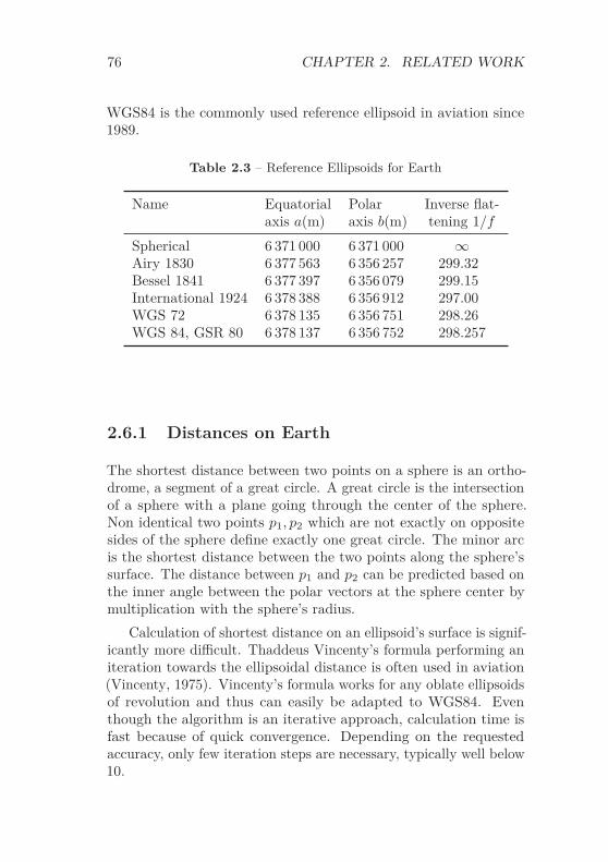
76 CHAPTER 2. RELATED WORK
WGS84 is the commonly used reference ellipsoid in aviation since1989.
Table 2.3 – Reference Ellipsoids for Earth
Name Equatorial Polar Inverse flat-axis a(m) axis b(m) tening 1/f
Spherical 6 371 000 6 371 000 ∞Airy 1830 6 377 563 6 356 257 299.32Bessel 1841 6 377 397 6 356 079 299.15International 1924 6 378 388 6 356 912 297.00WGS 72 6 378 135 6 356 751 298.26WGS 84, GSR 80 6 378 137 6 356 752 298.257
2.6.1 Distances on Earth
The shortest distance between two points on a sphere is an ortho-drome, a segment of a great circle. A great circle is the intersectionof a sphere with a plane going through the center of the sphere.Non identical two points p1, p2 which are not exactly on oppositesides of the sphere define exactly one great circle. The minor arcis the shortest distance between the two points along the sphere’ssurface. The distance between p1 and p2 can be predicted based onthe inner angle between the polar vectors at the sphere center bymultiplication with the sphere’s radius.
Calculation of shortest distance on an ellipsoid’s surface is signif-icantly more difficult. Thaddeus Vincenty’s formula performing aniteration towards the ellipsoidal distance is often used in aviation(Vincenty, 1975). Vincenty’s formula works for any oblate ellipsoidsof revolution and thus can easily be adapted to WGS84. Eventhough the algorithm is an iterative approach, calculation time isfast because of quick convergence. Depending on the requestedaccuracy, only few iteration steps are necessary, typically well below10.

2.6. GEODETIC EARTH SYSTEMS 77
2.6.2 Map Projection
This section describes some widely used map projection techniquesto map a spherical/ellipsoidal Earth system on a 2D plane. Chap-ter 4 explains how the conflict detection algorithm of chapter 3is adapted for usage with geodetic Earth systems based on thesemappings. There is no optimum projection, every mapping createsdistortions.
2.6.2.1 Sinusoidal Projection
The sinusoidal projection (also known as Mercator equal-area pro-jection, fig. 2.25) is a pseudo-cylindrical projection preserving thearea (Snyder, 1987). It shows relative sizes accurately, but distortsshapes and directions. The transformation from sphere (ϕ, λ) intoplane (x, y) coordinates is simple:
x = (λ − λ0) · cos(ϕ), y = ϕ (2.2)
λ0 is the central meridian
2.6.2.2 Mercator Projection
The Mercator projection (fig. 2.26) is a cylindrical map projection.Since it represents loxodromes (i. e., lines crossing all meridiansof longitude at the same angle) with constant course, it is thestandard map projection for nautical purposes. The Mercatorprojection preserves well angles and shapes of small objects, butdistorts larger objects. The scale increases from the Equator to thepoles, where it is infinite.
x = (λ − λ0) , y = ln[tan
(π
4+
ϕ
2
)](2.3)
λ0 is the central meridian
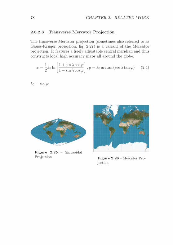
78 CHAPTER 2. RELATED WORK
2.6.2.3 Transverse Mercator Projection
The transverse Mercator projection (sometimes also referred to asGauss-Krüger projection, fig. 2.27) is a variant of the Mercatorprojection. It features a freely adjustable central meridian and thusconstructs local high accuracy maps all around the globe.
x =12
k0 ln[
1 + sin λ cos ϕ
1 − sin λ cos ϕ
], y = k0 arctan (sec λ tan ϕ) (2.4)
k0 = sec ϕ
Figure 2.25 – SinusoidalProjection Figure 2.26 – Mercator Pro-
jection

2.6. GEODETIC EARTH SYSTEMS 79
Figure 2.27 – Transverse Mercator Projection

80 CHAPTER 2. RELATED WORK

Chapter 3Conflict Detection
Efficient algorithms are required to perform conflict detection forcomplex problems in a reasonable time. Several algorithms alreadyexist realizing high performance conflict detection, but usuallycome from different application areas with different environmentalconstraints.
The constraints for conflict detection in aviation are:
• Objects (e. g., aircraft) and their occupied space are smallcompared to the containment area (i. e. airspace). Typicalshapes of occupied space are cylinders with diameters of5 NM and heights of 1000 ft (fig. 1.1 on page 25). Althoughthe underlying non-linear coordinate system increases effort,overall collision detection in narrow phase is simple.
• Aircraft are typically staggered vertically with valid 1000 ftseparation. Approximation of the separation cylinder with asphere would result in a high false-positive rate.
• Aircraft move fast in airspace, typically resulting in conflictswith short durations. Aircraft move on continuous trajectories.Due to their high speed compared to their size discretizationof time should be avoided.
81

82 CHAPTER 3. CONFLICT DETECTION
• 4D airspace is sparsely filled with objects only. However,designated areas of airspace are crowded, especially areas inthe vicinity of airports.
• No-fly zones with complex 4D shapes are additional hazardsin airspace that shall be respected.
• Different conflict metrics may apply for different parts ofairspace.
• WGS84 distance metrics are complex to calculate (section 2.6).
• Even though the trajectories of aircraft are assumed to bewell-known for whole flights, updates of trajectories shouldbe possible with low costs.
• The expected number of conflicts in aviation scenarios isusually low. Even a dense scenario with unaligned trajectoriesusually yields less than one conflict per aircraft on average(compare table 4.2 on page 143).
• The algorithm should allow to dynamically add (e. g., newscheduled departures) and delete (e. g., canceled flights) ob-jects.
Since already pairwise comparisons of trajectories are compu-tationally expensive, an efficient broad phase avoiding pairwiseconflict detections in the first place is desirable. BVH as describedin section 2.2.7 allows a very fast first comparison between twotrajectories based on their bounding boxes, but does not skip thecomparison completely.
Applying KDS from section 2.2.8 requires the generation ofcertificates and prediction of events for aircraft. Furthermore, aKDS implementation for three dimensions seems to be ambitious (noknown 3D-implementation yet), especially with cylindrical shapedobjects.
Also the sweep and prune approaches described in section 2.2.9are not reasonable for the given problem. Handling the dimensionsone-by-one would result in a large number of altitude intersectionseach generating an event even if the objects are laterally wellseparated.

3.1. DEFINITIONS 83
The 3D subdivision described in section 2.4.3 using octrees ispromising, but a static subdivision of worldwide airspace with areasonable memory equipped computer would allow a flat tree only.Furthermore, it is not intuitive to skip one dimension (Koeners andde Vries skipped altitude while Hildum and Smith skipped time),as long as no memory constraints exist.
The algorithm developed in this thesis is based on N-dimensionalbisection. The fundamental idea is based on an early exclusionof conflict checking whenever a conflict is obviously impossible.In 4D-airspace, a conflict check may be excluded if two aircraftare separated laterally (fig. 3.1). Separation is ensured either inx-direction, y-direction, or a combination of both. If two aircraftfly in significantly different altitudes, they are separated vertically(fig. 3.2). Finally, aircraft are allowed to fly exactly the same routewith exactly the same vertical profile if they only fly at differenttimes (fig. 3.3).
3.1 Definitions
This section gives some definitions for basic objects referred towithin the following chapters.A line segment in N-dimensional space is defined as a point set bytwo points �p1 and �p2:
L(�p1, �p2) = {�x : �x = �p1 + μ (�p2 − �p1)} (3.1)
�x, �p1, �p2 ∈ RN
0 ≤ μ ≤ 1, μ ∈ R
A trajectory is defined as a set of connected line segments by kpoints �p1, . . . , �pk:
T (�p1, . . . �pk) = L(�p1, �p2) ∪ L(�p2, �p3) ∪ . . . ∪ L(�pk−1, �pk) (3.2)

84 CHAPTER 3. CONFLICT DETECTION
Figure 3.1 – Lateral Separa-tion between 4D-Trajectories
Figure 3.2 – VerticalSeparation between 4D-Trajectories
Figure 3.3 – Time - basedSeparation between 4D-Tra-jectories
Figure 3.4 – 4D-Hypercube(Tesseract)
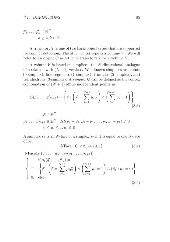
3.1. DEFINITIONS 85
�p1, . . . , �pk ∈ RN
k ≥ 2, k ∈ N
A trajectory T is one of two basic object types that are supportedfor conflict detection. The other object type is a volume V . We willrefer to an object O as either a trajectory T or a volume V .
A volume V is based on simplices, the N -dimensional analogueof a triangle with (N + 1) vertices. Well known simplices are points(0-simplex), line segments (1-simplex), triangles (2-simplex), andtetrahedrons (3-simplex). A simplex S can be defined as the convexcombination of (N + 1) affine independent points as
S(�p1, . . . , �pN+1) =
{�x :
(�x =
N+1∑i=1
μi�pi
)∧
(N+1∑i=1
μi = 1
)}
(3.3)
�x ∈ RN
�p1, . . . , �pN+1 ∈ RN : det(�p2 − �p1, �p3 − �p1, . . . , �pN+1 − �p1) �= 0
0 ≤ μi ≤ 1, μi ∈ R
A simplex s1 is an N -face of a simplex s2 if it is equal to one N -faceof s2.
NFace : S × S → {0, 1} (3.4)
NFace(s1(�q1, . . . , �qN ), s2(�p1, . . . , �pN+1)) =⎧⎪⎪⎪⎨⎪⎪⎪⎩
1,
if s1(�q1, . . . , �qN ) ={�x :
(�x =
N+1∑i=1
μi�pi
)∧
(N+1∑i=1
μi = 1
)∧ (∃j : μj = 0)
}
0, else(3.5)

86 CHAPTER 3. CONFLICT DETECTION
�x ∈ RN
j ∈ {1, . . . , N + 1}�p1, . . . , �pN+1 ∈ R
N
�q1, . . . , �qN ∈ RN
0 ≤ μi ≤ 1, μi ∈ R
Finally, a volume V is defined as a homogeneous simplicial N -complex recursively by a set of simplices connected by faces ofdimension N-1:
V (s1, . . . , sk) ={
s1, if k = 1V (s1, . . . , sk−1) ∪ sk, if k > 1 (3.6)
∃j : (NFace(sj ∩ sk, sj) = 1) ∧ (NFace(sj ∩ sk, sk) = 1)s1, . . . , sk ∈ S(�p1, . . . , �pN+1)
j ∈ {1, . . . , k − 1}
The bisection algorithm described in this chapter operates on tiles.A tile A is a subset of a N-dimensional Euclidean space defined bytwo vectors holding minimum (�amin) and maximum (�amax) valuesfor each dimension.
A(�amin,�amax) = {�x : (amin,i ≤ xi ≤ amax,i) for all i ∈ {1, . . . , N}}(3.7)
�x,�amin,�amax ∈ RN
A similar definition can be given by the Cartesian product of Nintervals:
A(�amin,�amax) = [amin,1, amax,1]×[amin,2, amax,2] × . . . ×[amin,N , amax,N ]
(3.8)
One dimension of an object can be defined to be a time dimension. Ifa time dimension is specified, let it be assigned to the last dimensionN of an object without loss of generality. Time τ then serves as

3.2. N-DIMENSIONAL CONFLICT 87
a common reference for conflict detection. Therefore, a trajectoryneeds to be one-dimensional along time axis and capable of beingparameterized by a time τ .
∃1(�x ∈ T ) : xN = τ (3.9)
�x ∈ RN
amin,N ≤ τ ≤ amax,N
This restriction does not account for volumes though, volumes canbe (N − 1)-dimensional along time. The functions V (τ) and T (τ)correspond to the volume/trajectory for the given time τ
V (τ) = {V (s′1, . . . , s′
m) ⊂ V (s1, . . . , sk) : s′i,N = τ
for all i ∈ {1, . . . , m}}(3.10)
T (τ) = {�x ∈ T : xN = τ} (3.11)
�x ∈ RN
O(τ) resolves to T (τ) or V (τ) for trajectories or volumes, respec-tively. The result of O(τ) has always full dimension N with the Nthdimension being constantly equal to τ in order to avoid differentdimensions in calculations.
3.2 N-Dimensional Conflict
This section defines if two objects are in conflict. It needs to bedistinguished if a time reference shall be taken into account, or ifall dimensions are treated equally.

88 CHAPTER 3. CONFLICT DETECTION
3.2.1 Conflicts without Time Reference
Two trajectories t1, t2 ∈ T are in conflict if the separation of trajec-tories is lower than a predefined mandatory separation �S in all Ndimensions.
∃(�p1 ∈ t1)∃(�p2 ∈ t2) : (|�p1 − �p2|i < Si) for all i ∈ {1, . . . , N}(3.12)
�pk ∈ RN , point on trajectory tk
�S ∈ RN , mandatory separation
A volume v1 ∈ V is in conflict with an object o1 if v1 containspartly o1.
∃�p1 : (�p1 ∈ o1) ∧ (�p1 ∈ v1) (3.13)
3.2.2 Conflicts with Time Reference
If a time axis is specified within the N-dimensional vector, it is usedas a common reference of all objects. Two trajectories t1, t2 ∈ Tare in conflict, if their distance at a common time τ is lower thanthe necessary separation �S in all N dimensions.
∃τ : |t1(τ) − t2(τ)|i < Si for all i ∈ {1, . . . , N} (3.14)
τ ∈ R, common time�S ∈ R
N , mandatory separation
A volume v1 ∈ V is in conflict with an object o1 ∈ (T ∪ V ) if v1contains partly o1 at a common time τ .
∃τ, �p1 : (�p1 ∈ o1(τ)) ∧ (�p1 ∈ v1(τ)) (3.15)
τ ∈ R, common time

3.3. N-DIMENSIONAL TILING ALGORITHM 89
The separation in time dimension is zero by definition. Therefore,time separation does not need to be checked explicitly. Nevertheless,the time component of �S shall be positive.
Obviously, a conflict with time reference is also a conflict withouttime reference for SN > 0 because the difference in time dimensionis zero. Therefore, data with time reference can be treated with bothalgorithms. Checking conflicts with time reference is a specializationof the standard check without time reference.
Setting SN > 0 to an arbitrary small epsilon
SN = ε (3.16)
ε > 0
provides identical results with and without time reference. However,there are good reasons to consider time separately:
• The mandatory separation �S is also used as minimal tile sizefor the bisection algorithm. Simply setting one dimension toε produces unwanted results.
• Having a common reference between all objects can be usedbeneficially as a speed-up by reducing necessary comparisons.
• Based on monotony of time dimension binary search can beapplied.
• The conflict tree size can be reduced significantly in timereference mode (section 3.3.3).
3.3 N-Dimensional Tiling Algorithm
Detecting N -dimensional conflicts in a large set of objects is a timeconsuming task. For example, Germany’s airspace is an operationarea of more than 10 000 flights on busy days, each flight representedby a high-precision 4D-trajectory with several hundred sampling
90 CHAPTER 3. CONFLICT DETECTION
points. Comparing each trajectory against each other without anyoptimization produces unacceptable response times.
In order to avoid extensive conflict detection, the provided algo-rithm separates objects by generating N -dimensional tiles holdingjust one object. The tiles are organized in a tree structure. Depend-ing on the number of dimensions N , one node of the tree has up to2N children.
Starting condition for the tiling algorithm is an N -dimensionalorthogonal tile being large enough to hold all objects in all dimen-sions in terms of a convex hull. Objects are treated by the algorithmconsecutively. In the beginning, this root tile is empty.
Objects are inserted in the root tile. The conflict detection isperformed directly on insertion. As soon as a tile (e. g., the roottile) is affected by more than one object, the tile is subdivided in alldimensions by adding up to 2N children. Figure 3.5 illustrates thesubdivision process for the one-, two-, and three-dimensional cases.Tile shape for the 4D-case is a 4D-hyperrectangle, its cubic versionalso known as tesseract(fig. 3.4). Table 3.1 gives an overview ontile shapes and their subdivision.
Table 3.1 – Overview on N-dimensional Bisection
Dimension Tile shape Number of tiles in depth1 2 3 m
1 Line 2 4 8 2m
2 Rectangle 4 16 64 4m
3 Rectangular box 8 64 512 8m
4 4D-Hyperrectangle 16 256 4096 16m
......
......
......
n n-D Hyperrectangle 2n 22·n 23·n 2m·n
Having in mind the aviation background, the 4-dimensionalcase is of particular interest. Therefore, fig. 3.6 depicts the sixteenfirst-level children of a tesseract.

3.3. N-DIMENSIONAL TILING ALGORITHM 91
>
Figure 3.5 – Bisection for 1-3 Dimensions
Figure 3.6 – First Level Bisection of Tesseract with 16 Children
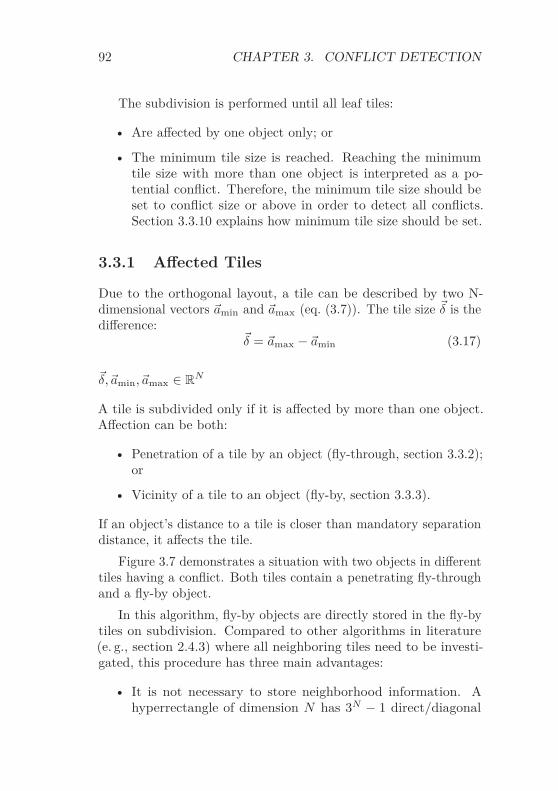
92 CHAPTER 3. CONFLICT DETECTION
The subdivision is performed until all leaf tiles:
• Are affected by one object only; or
• The minimum tile size is reached. Reaching the minimumtile size with more than one object is interpreted as a po-tential conflict. Therefore, the minimum tile size should beset to conflict size or above in order to detect all conflicts.Section 3.3.10 explains how minimum tile size should be set.
3.3.1 Affected Tiles
Due to the orthogonal layout, a tile can be described by two N-dimensional vectors �amin and �amax (eq. (3.7)). The tile size �δ is thedifference:
�δ = �amax − �amin (3.17)
�δ,�amin,�amax ∈ RN
A tile is subdivided only if it is affected by more than one object.Affection can be both:
• Penetration of a tile by an object (fly-through, section 3.3.2);or
• Vicinity of a tile to an object (fly-by, section 3.3.3).
If an object’s distance to a tile is closer than mandatory separationdistance, it affects the tile.
Figure 3.7 demonstrates a situation with two objects in differenttiles having a conflict. Both tiles contain a penetrating fly-throughand a fly-by object.
In this algorithm, fly-by objects are directly stored in the fly-bytiles on subdivision. Compared to other algorithms in literature(e. g., section 2.4.3) where all neighboring tiles need to be investi-gated, this procedure has three main advantages:
• It is not necessary to store neighborhood information. Ahyperrectangle of dimension N has 3N − 1 direct/diagonal

3.3. N-DIMENSIONAL TILING ALGORITHM 93
Figure 3.7 – Objects in Different Tiles having a Lateral Conflict
neighbors. For a 4D map, this would increase necessarymemory by 34 − 1 = 80 pointers per tile – 640 B on 64 bitcomputer.
Identifying neighbors dynamically, without storing them, isnot an option since neighbor search is too slow.
• Keeping neighborhood information consistent is a complextask and computational expensive in a dynamic heterogeneoustree.
• In contrast to a static array, it is not feasible to check forconflicts against all candidates from neighboring tiles in adynamic tree. After the first subdivision of root tile, everytile is a direct neighbor of every other tile. Thus, conflictcheck has to be limited on objects close to the border.
3.3.2 Check for Penetration
A tile A is penetrated by an object O if at least one point of O iswithin A.
∃(�p ∈ O) : (�p ∈ A) (3.18)
This equation is good for the sake of mathematical definition, butsince objects are defined as infinite point sets, it cannot be checkeddirectly by a computer program.
Due to the orthogonality of the underlying coordinate system,penetration of a tile by an object can be re-formulated allowing

94 CHAPTER 3. CONFLICT DETECTION
an implementation on a computer. An object penetrates an N-dimensional tile if:
• All points of the object are within the tile; or
• At least one boundary of the object intersects with one of the2 · N tile boundaries; or
• The object contains the complete tile (only relevant for vol-umes).
Bullet one is easy to verify. Only one (e. g., the first) point �p of theobject needs to be checked.
∀i : amin,i ≤ pi ≤ amax,i (3.19)
i ∈ {1, . . . , N}�p ∈ R
N
If the tile encloses the test point �p, the object obviously penetratesthe tile A. If the result is negative, not all points of O lie in thetile.
Bullet three can be checked with comparable effort. Only onepoint �p (e. g., �amin) of the tile needs to be checked to be within avolume V .
(�p ∈ V (s1, . . . , sk)) ⇔ ∃i : �p ∈ si (3.20)
i ∈ {1, . . . , k}
Again, if the volume contains the point �p, the volume obviouslypenetrates the tile A. If the result is negative, not all points of Aare located within the object.
If both checks are negative, the intersection of tile and ob-ject boundaries need to be checked. For each dimension, an N -dimensional tile has a lower and an upper boundary. Since tiles areaxis-aligned, the shape of tile boundaries has one dimension lessthan the tile itself (table 3.2).

3.3. N-DIMENSIONAL TILING ALGORITHM 95
Table 3.2 – Boundaries of N-dimensional Tiles
Dim. Tile Boundary Number ofshape shape boundaries
1 Segment Point 22 Rectangle Segment 43 Rectangular box Rectangle 64 4D-Hyperrect. Rectangular box 8...
......
...n n-D Hyperrect. (n-1)-D Hyperrect. 2 · n
The final check whether object boundaries intersect with thetile depends on the object type. The corresponding algorithms areexplained in section 3.4.1 for trajectories and within section 3.4.2for implemented volumes.
3.3.3 Check for Vicinity
The vicinity test can be performed easiest by using a dilatation ofthe tile. Instead of checking distances to a given tile, the tile isextended by the separation margins. Figure 3.8 depicts a trajectorythat penetrates both the tile itself and the extended fly-by tile.Based on the two N-dimensional vectors �amin and �amax describingthe tile, the dilatation tile can be described by
�a′min =
(�amin − �S
)and �a′
max =(�amax + �S
)(3.21)
amin, amax, a′min, a′
max ∈ RN
�S ∈ RN , mandatory separation
Thus, vicinity check can be performed as described in section 3.3.2using �a′
min and �a′max.
In time reference mode, a dilatation of time is not necessarybecause proximity in time is not relevant for the conflict decision.

96 CHAPTER 3. CONFLICT DETECTION
Figure 3.8 – Trajectory in Fly-Through and Fly-By Zone

3.3. N-DIMENSIONAL TILING ALGORITHM 97
Penetrated by one aircraft
Penetrated by one aircraft
Affected by two aircraft
Figure 3.9 – No Conflict without Fly-Through Object in CenterTile
Objects are only compared at identical times τ . Avoiding thedilatation in time provides a significant decrease of used memoryand significant increase of calculation speed. For the aviationexample, this results in ∼25 % better run-time and ∼40 % lessmemory. Therefore, we set for the time reference mode
a′min,N = amin,N and a′
max,N = amax,N (3.22)
A tile contains a potential conflict only if:
• It is affected by at least two objects; and
• Penetrated by at least one object.
A tile with fly-by objects, only, does not contain any conflicts(fig. 3.9).
3.3.4 Symmetric Simplification
Figure 3.7 on page 93 illustrates that conflicts are detected twice.Both tiles displayed contain a fly-by and a fly-through object, each.While this is technically not a problem since detected conflicts aremerged, symmetric situations are both memory and time consuming.Thus, the idea of this section is avoiding symmetric situations byskipping the fly-by object in one of the two tiles.
A clear rule needs to be defined in order to ensure that fly-by situations are at least taken into account by one tile. The

98 CHAPTER 3. CONFLICT DETECTION
implemented method skips fly-by objects by their relative positionto the tile. For each dimension i it is checked whether the tile-relevant part of the object is below the corresponding amin,i or aboveamax,i. If no dimension is found where the object is constantly belowor above the corresponding tile dimension, the fly-by object is kept,resulting in a potential extra effort.
Otherwise, the fly-by object is kept only if it is constantly abovethe maximum tile value for at least one dimension. Focusing onthe left tile in fig. 3.7, the right trajectory is constantly above themaximum x-value of the left tile. Concerning the right tile, theleft trajectory is constantly below the x-value of the right tile andthus is omitted. For the aviation example, this technique improvesrun-time by ∼15 % and decreases memory usage by ∼25 %.
3.3.5 Full Containment
If a volume V contains one point of a tile A and volume’s boundariesdo not intersect the tile’s boundaries, the volume V includes thecomplete tile.
∀�x ∈ A ⇒ �x ∈ V (3.23)
Every other object also penetrating this tile has a real conflictwith the volume V . No extra information concerning volume Vis gained with further subdivision of the appropriate internal tile.Therefore, volumes containing whole tiles can be treated as a fly-byobject for the tiling decision.
For example, if only one aircraft flies in German airspace, andthe trajectory is checked for conflict against a volume representingGerman airspace, subdivision only needs to be done until one tile iscompletely inside German airspace and also contains the trajectory.
Figure 3.10 depicts two aircraft flying through the volume object"German airspace". The southern aircraft enters and leaves Germanyat the east-boundaries. The northern aircraft starts within theGerman volume, and leaves the volume through the upper boundary.Once a tile contains a trajectory and the tile is completely inside theGerman volume, it is not necessary to perform further subdivision,although the tile technically is penetrated by two objects.
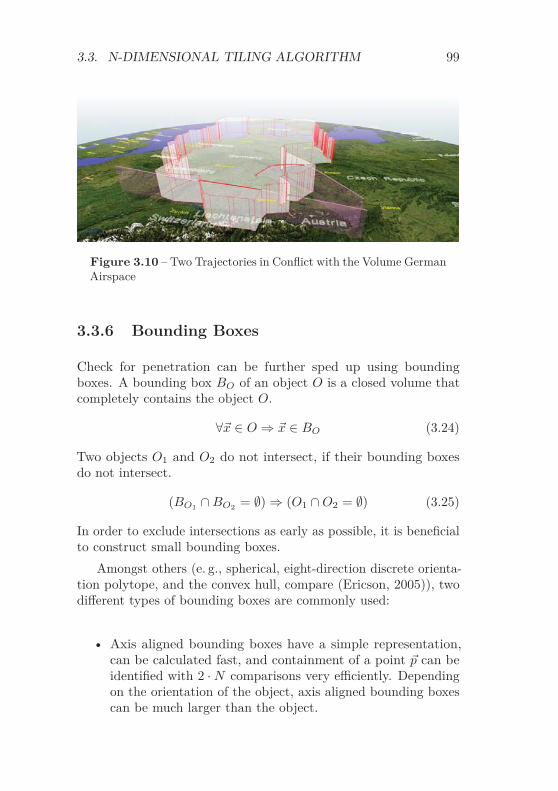
3.3. N-DIMENSIONAL TILING ALGORITHM 99
Figure 3.10 – Two Trajectories in Conflict with the Volume GermanAirspace
3.3.6 Bounding Boxes
Check for penetration can be further sped up using boundingboxes. A bounding box BO of an object O is a closed volume thatcompletely contains the object O.
∀�x ∈ O ⇒ �x ∈ BO (3.24)
Two objects O1 and O2 do not intersect, if their bounding boxesdo not intersect.
(BO1 ∩ BO2 = ∅) ⇒ (O1 ∩ O2 = ∅) (3.25)
In order to exclude intersections as early as possible, it is beneficialto construct small bounding boxes.
Amongst others (e. g., spherical, eight-direction discrete orienta-tion polytope, and the convex hull, compare (Ericson, 2005)), twodifferent types of bounding boxes are commonly used:
• Axis aligned bounding boxes have a simple representation,can be calculated fast, and containment of a point �p can beidentified with 2 · N comparisons very efficiently. Dependingon the orientation of the object, axis aligned bounding boxescan be much larger than the object.

100 CHAPTER 3. CONFLICT DETECTION
Figure 3.11 – Axis Aligned vs. Object Oriented Bounding Box
• Object oriented bounding boxes have a more complex rep-resentation, are more difficult to calculate, and containmentcheck is slower. Object oriented bounding boxes approximatean object usually with a smaller volume than axis alignedbounding boxes.
Figure 3.11 shows an example for both axes aligned (light grey) andobject oriented bounding box (light green) types in 2D. If objects’sizes are big compared to distances between objects, and they areusually not aligned to axis, object aligned bounding boxes mightbe beneficial. This approach focuses on the simpler and faster axisaligned bounding boxes:
BO(bmin, bmax) ={�x ∈ O : (bmin,i ≤ xi ≤ bmax,i) for all i ∈ {1, . . . , N}} (3.26)
Conflicts can be excluded early by a non-intersection of boundingboxes. Since the geometry of a bounding box is similar to that ofa tile, comparisons can be performed inter objects and between

3.3. N-DIMENSIONAL TILING ALGORITHM 101
objects and tiles. Two bounding boxes b1 and b2 do not intersect if∃i : (b1max,i < b2min,i) ∨ (b1min,i > b2max,i) (3.27)
i ∈ {1, . . . , N}
3.3.7 Building the Tree
Task of the conflict tree is to represent all objects in a consistentway supporting a fast detection of separation violations.
Concerning the implementation, the conflict detection moduleholds separately:
• A list of all objects.
• The tree structure with references to the objects.
• A list of conflicts between stored objects.
A major invariant of the software is that all entries are consistentwhen the module is accessible from the outside. Therefore, when anew object is added to the tree, the object is added to the internalobject list, all necessary tiles are generated immediately, and finallythe list of conflicts is updated.
When a tile needs to be subdivided because it is affected byat least two objects with at least one penetration, all 2N childrenneed to be checked for affection by the new object. Some of thechildren tiles might already exist from earlier inserted objects, allother affected tiles need to be generated. This recursive process isperformed until further subdivision is not required or separationsize is reached.
If a leaf is completely inside of a/some volume(s) (section 3.3.5),a conflict with the volume(s) is detected. If one of the leaves hasminimum tile size �S a potential conflict is detected with all otherobjects of the tile (section 3.5). Otherwise, the object is proven tobe free of conflict.

102 CHAPTER 3. CONFLICT DETECTION
3.3.8 Monotonic Dimensions
When adding a new object, all dimensions are checked for monotony.If a dimension increases or is partly constant with increasing index,the dimension is monotonically increasing. If a dimension decreasesor is partly constant with increasing index, the dimension is mono-tonically decreasing. In time reference mode, the time dimensionof an implemented trajectory object is always strictly increasingdue to eq. (3.9). But also other dimensions can be monotonic,for instance a trajectory going strictly from West to East has amonotonic longitudinal axis.
When identified, monotony can be used beneficially for speedingup intersection calculation with an axis-oriented plane. Instead ofchecking each trajectory segment to have vertices on opposite sidesof the plane, binary search can be applied to identify the correctsegment directly.
3.3.9 Balancing the Tree
When configuring the tree, dimensions are usually independent.Value range and mandatory separation might differ significantlybetween dimensions. Dimensions can even have different physicalunits. The user has to ensure that units are used consistently foreach dimension. Based on the starting interval I = [�Imin, �Imax] andthe separation �S, the number of subdivisions �D can be defined as
Di = log2 ((Imax,i − Imin,i) /Si) (3.28)
�D, �Imin, �Imax, �S ∈ RN
i ∈ {1, . . . , N}
If the resulting vector has a big range max(Di) − min(Di), theminimum tile size is reached in different tree depths. Although thisis technically not a problem, such behavior produces an unbalancedtree that subdivides deeper tiles in a subset of dimensions only.
If such behavior is unwanted, the software provides an automaticbalancing functionality. When the interval I and minimum tile size
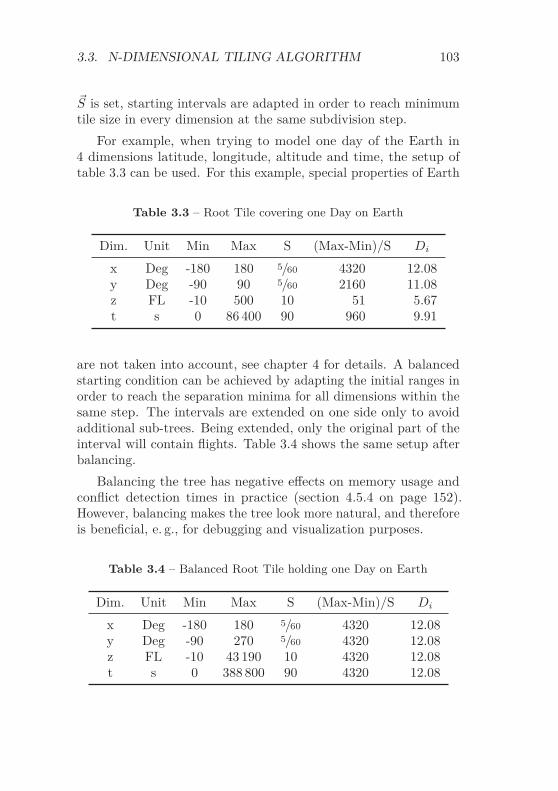
3.3. N-DIMENSIONAL TILING ALGORITHM 103
�S is set, starting intervals are adapted in order to reach minimumtile size in every dimension at the same subdivision step.
For example, when trying to model one day of the Earth in4 dimensions latitude, longitude, altitude and time, the setup oftable 3.3 can be used. For this example, special properties of Earth
Table 3.3 – Root Tile covering one Day on Earth
Dim. Unit Min Max S (Max-Min)/S Di
x Deg -180 180 5/60 4320 12.08y Deg -90 90 5/60 2160 11.08z FL -10 500 10 51 5.67t s 0 86 400 90 960 9.91
are not taken into account, see chapter 4 for details. A balancedstarting condition can be achieved by adapting the initial ranges inorder to reach the separation minima for all dimensions within thesame step. The intervals are extended on one side only to avoidadditional sub-trees. Being extended, only the original part of theinterval will contain flights. Table 3.4 shows the same setup afterbalancing.
Balancing the tree has negative effects on memory usage andconflict detection times in practice (section 4.5.4 on page 152).However, balancing makes the tree look more natural, and thereforeis beneficial, e. g., for debugging and visualization purposes.
Table 3.4 – Balanced Root Tile holding one Day on Earth
Dim. Unit Min Max S (Max-Min)/S Di
x Deg -180 180 5/60 4320 12.08y Deg -90 270 5/60 4320 12.08z FL -10 43 190 10 4320 12.08t s 0 388 800 90 4320 12.08

104 CHAPTER 3. CONFLICT DETECTION
3.3.10 Broad Phase vs. Narrow Phase
The N -dimensional tiling algorithm performs the broad phase anddoes not identify real conflicts but potential conflicts, only. Thefinal conflict check needs to be performed afterwards in the narrowphase. Thus, all real conflicts are handled twice:
• First by the tiling algorithm with low costs CT .
• Second by the final conflict check that might be very expensivein terms of calculation costs CF .
If the likelihood of conflicts PC is low, exclusion of many non-conflicting situations is beneficial. Conflict likelihood increaseswhen coming further down in the tiling tree. The total costs Ccalculate as
C = PC · (CT + CF ) + (1 − PC) · CT (3.29)
PC ∈ R, 0 ≤ PC ≤ 1 (conflict likelihood)CT , CF > 0, CT � CF (costs)
Using the tiling algorithm is beneficial as long as C is lower thanCF . Obviously this strongly depends on CT
CFand PC . Therefore,
the size of the smallest tile does not necessarily need to be theconflict detection size. If conflicts have a high likelihood and CT
CFis
close to one, smallest tile size should be bigger than the mandatoryseparation size. Therefore, the tiling algorithm is called with anincreased requested separation �S, while the final conflict check(section 3.5) uses the original separation.
Especially in time reference mode (section 3.2.2) time separationcan be freely adjusted in order to achieve best possible detectionperformance.

3.3. N-DIMENSIONAL TILING ALGORITHM 105
3.3.11 Memory Limitation
The bisection algorithm in its basic version performs a time-memorytradeoff. In order to reach fast computation times, it uses a tremen-dous amount of memory. Depending on the problem and computerhardware, the algorithm might exceed physical available memory.Therefore, two mechanisms are implemented helping to adjust thetradeoff:
• Static: By means of a max tree depth, the user can limitthe refinement of the tree. The algorithm does not generatenodes that exceed the defined tree depth. This method is anindicator only to reduce memory size; it does not allow toexplicitly name a memory limit.
• Dynamic: The algorithm provides a feature of monitoringmemory usage against available system memory. If the ratioexceeds a given value (e. g., 70 %), it automatically decreasesthe depth of tree by one. Depending on the tree size andespecially on the number of leaves, this operation might takesome time. However, it prevents memory problems on reducedhardware. The tree depth reduction is performed every timethe given ratio is exceeded.
3.3.12 Tile Knowledge
As already mentioned in section 3.3.7, each tile stores references tothe objects affecting it including the type of affection (fly-throughor fly-by, and if the object contains the complete tile). In order toincrease algorithm’s speed, more information is stored in tiles.
When verifying tile affection, the segments of trajectories arechecked successively. Negative results can beneficially be used forfurther subdivisions. Trajectory segments not affecting a node willalso not affect any of its children because every child is a real subsetof its father.
Therefore, the interval affecting a tile is stored for each object.In the beginning, this interval is set to [1, K] with K being the

106 CHAPTER 3. CONFLICT DETECTION
number of trajectory definition points. If possible this interval isreduced when going down the tree.
3.4 Supported Objects
The implemented software provides two objects in its current version:trajectories and a special implementation of volumes, the polygonvolume. A variation of a polygon volume, the moving polygonvolume, is described in section 3.4.3. Further objects can be definedeasily if necessary.
3.4.1 N-Dimensional Trajectories
The trajectories supported by the module directly implement as alist of N -dimensional points connected by line segments, as definedin eq. (3.2), page 83. Concerning the penetration check defined insection 3.3.2, one boundary of the object intersects with one of the2 · N tile boundaries if an edge of the trajectory intersects with atile boundary. Edges E can be identified for trajectories as the linesegments from eq. (3.2). An object’s edge E intersects with a tileboundary if corresponding vertices eb and ee are on opposite sidesof the boundary
∃i : (eb,i − bi) ∗ (ee,i − bi) ≤ 0 (3.30)
i ∈ {1, . . . , N}�b ∈ {�amin,�amax}
�eb, �ee ∈ RN being begin and end of edge E
in one dimension and the intersection point �p of the edge with theboundary �b for the same dimension i
�p =bi − eb,i
ee,i − eb,i∗ �ee +
(1 − bi − eb,i
ee,i − eb,i
)∗ �eb (3.31)

3.4. SUPPORTED OBJECTS 107
�b ∈ RN
�eb, �ee ∈ RN being begin and end of edge E
i ∈ {1, . . . , N}
is within the tile in all dimensions.If at least one edge intersects with a tile boundary, the object
penetrates the tile. If:
• Not all points of the trajectory are in the tile; and
• No edge intersects with a tile boundary;
it does not penetrate the tile.
3.4.2 N-Dimensional Volumes
Volumes are not implemented as generic as in eq. (3.6). Reasonsfor defining volumes another way are:
• Simplicial complexes are not the most intuitive way to imaginea volume.
• Simplicial complexes have more degrees of freedom than atypical user needs.
• Segmentation of a volume into simplices is a non-trivial taskfor humans, especially for high dimensions.
• Intersection of simplicial complexes with tiles is complex forhigh dimensions.
Instead of generic simplicial complexes, the implementation isbased on simple 2D-polygons P. We define 2D-polygons P as acomplex of 2-simplices (i. e., triangles, compare eqs. (3.3) to (3.6)):
P(s1, . . . , sk) ={
s1, if k = 1P (s1, . . . , sk−1) ∪ sk, if k > 1 (3.32)

108 CHAPTER 3. CONFLICT DETECTION
∃j : (NFace(sj ∩ sk, sj) = 1) ∧ (NFace(sj ∩ sk, sk) = 1)s1, . . . , sk ∈ S (�p1, �p2, �p3)
j ∈ {1, . . . , k − 1}
Every dimension higher than 2 is defined by an interval, beingconstant for all points of the 2D polygon. Thus, a polygon volumeV is defined as the Cartesian product
V = P ×[�Imin, �Imax
](3.33)
�Imin, �Imax ∈ RN-2
A volume as described above intersects with a tile if all N −2 intervaldimensions intersect with the corresponding tile intervals, and thepolygonal part intersects with the 2D-part of the tile. Therefore,fastest way to exclude an intersection is to find a dimension j where
(Imin,j > amax,j+2) ∨ (Imax,j < amin,j+2) (3.34)
j ∈ {1, . . . , N − 2}�amin,�amax ∈ R
N being the tile limitations
If the tile includes all intervals, the polygon’s outline needs to bechecked. While the polygon’s outline would need to be extractedexplicitly from the point set eq. (3.32), the software implementationcreates polygons from a given outline. Thus, the outline is explicitlyavailable.
Since the polygon’s outline has the same format as a (closed)2D-trajectory (section 3.4.1), the same algorithms can be applied.Having in mind the check for one point of the volume being partof the tile, and for one point of the tile being within the volume(section 3.3.2) validation of intersection between tiles and polygonvolumes are rather fast.

3.4. SUPPORTED OBJECTS 109
As written before (section 3.3.5), full containment is of interestfor polygon volumes. Full containment can easily be identified. Atile is completely within a polygon volume if:
• One point of the tile is within the polygon volume; and
• The polygon volume does not intersect with the tile boundaries
Due to the application of airborne traffic, the software is con-figured to detect conflicts involving trajectories, only. Therefore,conflicts between volumes are omitted, only trajectory/trajectoryand trajectory/volume situations are of relevance.
Based on polygon volumes, more complex constructs can bedefined by combination. Staggering polygon volumes above eachother allows to define volumes that change extension with altitude(e. g., for representation of cumulonimbus clouds that usually havea flat layer at the top). Defining different polygon volumes for shortconnected time periods represents a volume changing shape in time(e. g., for representation of ash-clouds).
3.4.3 N-Dimensional Moving Volumes
For the time referenced conflict detection, an extension of polygonvolumes is provided by the ability of assigning a trajectory TV to avolume V. This trajectory defines an offset in all (N-1) dimensionsas a function of time. Thus, the trajectory adds the capabilityof moving the polygon along an assigned path. The original timeinterval of V, if defined, is ignored. In accordance with eq. (3.33), apolygon volume V(τ) for time τ is defined as the Cartesian product
V(τ) = P ×[�Imin, �Imax
]× [0, 0] + TV(τ) (3.35)
�Imin, �Imax ∈ RN-3
TV ⊂ RN is the assigned trajectory
The penetration detection works similar to that described for thenon-moving polygon volume described in section 3.4.2 while respect-

110 CHAPTER 3. CONFLICT DETECTION
ing the movement induced by the assigned trajectory. A boundingbox intersection trial between the tile and the bounding box of thepolygon volume for the time interval [amin,N , amax,N ] allows a quickcheck if a situation represents a possible collision, at all. Whenpositive, it needs to be verified if:
• The moving polygon contains the whole tile. One point ofthe tile (e. g., the center point 0.5 · (�amin +�amax)) needs to bechecked to be inside the polygon.
• The tile contains the whole polygon. One point of the polygonneeds to be checked to be inside the tile.
• The tile intersects with the moving polygon. If both testsabove provide negative results, polygon intersection needsto be tested. The intersection test also helps to calculatecomplete containment (section 3.3.5). If one point of thepolygon is inside the tile (see above) and the tile does notintersect with the polygon volume, the tile is completely withinthe polygon volume.
A moving polygon volume V(τ) is in conflict with a tile A if
∃τ : ∃�x : (�x ∈ V(τ)) ∧ (�x ∈ A) (3.36)
τ ∈ {amin,N , amax,N } ∧ (∃1�y ∈ TV : yN = τ)
However, checking the intersection between a volume and a tile forevery time τ is not possible that way on a computer. Discretizationof time is necessary, but also introduces several problems:
• Discretization reduces the accuracy of results. If a situationof interest is active for a very short time period, the resolutionof discretization needs to be good enough to detect the issue.
• High resolution discretization results in many computationalexpensive calculations. Especially with large tiles (i. e., thetiles close to the tree root) and long trajectories performancewould be low using straight forward discretization.

3.4. SUPPORTED OBJECTS 111
Figure 3.12 – Shape Generated by Moving Polygon
Figure 3.13 – Shape Generated by Less Symmetric Polygon
Therefore, another approach is chosen to calculate intersections.Figure 3.12 shows the blue shape generated by the red moving poly-gon in 2D along two trajectory segments in black/white. The bluecorridor represents the polygon along the two trajectory segments.The only values of interest for the corridor are the points withbiggest distance back and front (along track), and left and right(cross-track) from the central trajectory. These values define a rect-angle in 2D and change from one segment to the next, dependingon the trajectory’s direction and polygon’s shape.
The idea is translating x/y into along/cross-track componentsand thus overlaying along-track distance and time. Figure 3.13shows a less symmetric polygon creating a different shape.

112 CHAPTER 3. CONFLICT DETECTION
Figure 3.14 – 3D-Corridor for Moving Polygon
The corridor can also be calculated vertically and for all otherhigher dimensions, see fig. 3.14. The corridor is an object oriented(i. e., trajectory segment oriented) bounding volume (compare sec-tion 3.3.6) for the moving polygon. That way, a conservativerepresentation of the moving polygon for a specified time intervalis provided.
Figure 3.15 illustrates the calculation of higher dimension’s cor-ridor sizes using the example of altitude. Since the vertical size of apolygon is constant for the whole polygon by definition, it is enoughto investigate the four corners of the red polygon volumes. Basedon the gradient z′ = (Δz/Δdistance) of the trajectory segment, thestandard altitude interval from start of trajectory segment needs tobe extended by:
• (AlongTrackBefore ∗ z′); and
• (AlongTrackBehind ∗ z′).

3.5. N-DIMENSIONAL CONFLICT DETECTION 113
Figure 3.15 – Generation of Vertical Corridor
Based on the calculated corridor, intersections with the tile(if any) can be found fast and easily. Therefore, the trajectorydefining the volume’s movement is intersected with all tile boundaryplanes. If the intersection point is closer to a tile boundary thanthe corridor’s size, the corridor intersects with the tile. Since thecross-track tile size depends on the trajectory segment direction,it is beneficial to center the trajectory in cross track directionin order to reach a symmetric (and thus no direction dependent)lateral corridor size. Figure 3.16 depicts an intersection of a movingpolygon volume with a tile. Even though the centered trajectorydoes not penetrate the tile boundaries, the intersection point withthe front plane of the tile marked by the red ball is close enough toindicate a possible conflict between tile and corridor.
Finally, the potential conflict needs to be verified to be a realconflict by searching an intersection between the volume and thetile. The potential conflict provides an appropriate time frame forthat verification. Since the search area now has very limited size,time can be discretized to small values, e. g., to one time unit.
3.5 N-Dimensional Conflict Detection
As explained above, output of the broad phase algorithm describedin section 3.3 represents a list of potential conflicts. Depending onthe application area, potential conflicts might not fulfill all condi-

114 CHAPTER 3. CONFLICT DETECTION
Figure 3.16 – Intersection between Moving Polygon and Tile Planemarked with Red Sphere

3.5. N-DIMENSIONAL CONFLICT DETECTION 115
Penetrated by two aircraftPenetrated by
one aircraftPenetrated by
one aircraft
Figure 3.17 – Two Non-conflicting Objects in same Tile
tions of a real conflict. In aviation, separation minima are typicallydefined as a 2D circle in latitude/longitude plane. Figure 3.17 showsa situation where one tile is penetrated by two aircraft. However,even if latitude and longitude of both flights are closer than the al-lowed 5 NM, they are separated with the circular metric mentionedbefore.
The narrow phase conflict detection check is also essential ifit was decided to reduce depth of the tree by stopping the broadphase process earlier (e. g., going down to a separation of 10 NMonly, compare section 3.3.10) or memory limits were reached (sec-tion 3.3.11).
Validating a potential conflict as a real conflict might be acomplex task. Therefore, this check is not done within the softwarecore, but the detection module expects a pointer to an externalfunction deciding if two given points are in conflict:
bool isRealConflict(point �p1, point �p2, trend �t1, trend �t2) (3.37)
�p1, �p2,�t1,�t2 ∈ RN
In time reference mode, the trends �t1 and �t2 hold the differentialcoefficient for points �p1 and �p2 along the corresponding trajectoriesbased on one time unit. Trends can be used if conflict situationdepends on current state of objects. In aviation, aircraft might bedefined to have a conflict depending on their vertical speed.
116 CHAPTER 3. CONFLICT DETECTION
The conflict function defined in eq. (3.37) is called for trajectoryobjects only, because volumes are checked with regard to penetra-tion, only.
Summarizing, once the tiling algorithms indicates potentialconflicts, these need to be verified as real conflicts. The finalconflict check depends on the involved object types and is describedin the following sections.
3.5.1 Conflict between Trajectories
Section 3.2.1 and section 3.2.2 define a real conflict situation withoutand with time reference respectively. In the following, the processof conflict validation based on potential conflicts is described fortrajectories.
3.5.1.1 Trajectory Conflict including Time Reference
Based on the identified potential conflict and the correspondingtile A, a τ fulfilling eq. (3.14) needs to be identified in the intervalτ ∈ [Amin,N , Amax,N ]. Since A is a leaf tile, the interval is rathersmall and can be searched with a small discretization in time. Assoon as the conflict function from eq. (3.37) turns true for one τ , aconflict is identified.
Once a conflict is identified, it is extended in time dimensionin order to get start and end of conflict. A minimum gap time Gbetween two conflicts ensures that two parallel trajectories withsmall position jitter are continuously in conflict when moving closeto mandatory separation �S.
The minimum gap time G is also useful for the process ofcalculating minimum and maximum conflict time. Starting fromthe conflict-proved time τ , the conflict function from eq. (3.37) ischecked at τ ± k · G with k = 1, 2, 3, . . .. When the conflict check isnegative, the step size is continuously reduced down to the foreseenresult accuracy. Figure 3.18 shows how conflict start and end areiteratively calculated starting at the conflict-proved time τ . Thisprocedure allows fast detection of the conflict interval. However,due to the discretization of time, this approach may leave gaps

3.5. N-DIMENSIONAL CONFLICT DETECTION 117
Conflictproved
time, start of iteration
Step sizeStep size Step size Step size
Figure 3.18 – Calculation of Start and End of Conflict
that are smaller than the minimum gap time G. Therefore, a finalmerging is necessary, see section 3.5.3.
3.5.1.2 Trajectory Conflict without Time Reference
Without time reference, a tile contains a conflict if two trajec-tories t1, t2 come closer than the given mandatory separation �S(eq. (3.12)). Therefore, the minimum distance between two tra-jectories needs to be calculated. Before calculating the distance,trajectories are normalized with �S in order to have a common metricfor all dimensions.
Based on the normalized trajectories, all relevant segments fromt1 are checked against all relevant segments from t2. Segments arerelevant if they affect the tile. If the result is less or equal 1 in eachdimension, the result is finally verified with the external conflictfunction eq. (3.37).
If conflicts are identified for multiple segments, they are merged.The trajectory point index for the first conflict partner is stored forlater use, see section 3.5.4 for details.

118 CHAPTER 3. CONFLICT DETECTION
3.5.2 Conflict between Trajectory and Volume
As mentioned before, a conflict between a volume and a trajectoryexists when the trajectory penetrates the volume. As for trajectories,the conflict detection procedure differs with regard to time referenceavailable or not.
3.5.2.1 Trajectory/Volume Conflict including Time Ref-erence
The conflict with time reference is comparable with the proceduredescribed in section 3.5.1.1. Instead of testing the conflict functionit is checked if the volume for time τ contains the trajectory point.
3.5.2.2 Trajectory/Volume Conflict without Time Refer-ence
In contrast to the inter-trajectory conflict detection described insection 3.5.1.2, conflict detection for volumes is not performedwithin tile boundaries only, but for the whole volume. Therefore,each segment of the trajectory is checked for intersection with thevolume boundaries. In addition, start and/or end of trajectorywithin the volume is stored as a conflict.
Based on that conflict list, conflicts are sorted according to thetrajectory point index and grouped to pairs. These pairs then holdentry and exit point of the polygon volume.
3.5.3 Conflict Merging
As described in section 3.5.1.1, the discretization of time mayproduce gaps that are smaller than the minimum gap time G.Figure 3.19 illustrates this behavior. Since the third time offsetpoints to a no-conflict situation, the conflict is limited to the left sideof the conflict gap. Another position of the conflict gap could haveproduced the correct result containing the whole conflict. However,taking the gap problem into account directly when calculating theconflict interval would be computational expensive.

3.5. N-DIMENSIONAL CONFLICT DETECTION 119
ConflictConflict
GapConflict
Minimum Gap
Minimum Gap
Minimum Gap
Minimum Gap
Figure 3.19 – Discretization of Time prevents Gap Jump
In order to ensure that no conflict gap is smaller than minimumgap size G a final merge is performed when a new conflict is identified.If another conflict already exists with identical conflict partnerscombined with a smaller distance to the new conflict than G, bothconflicts are merged.
Having knowledge about the extent of conflicts helps with earlyocclusion of already detected conflicts. The conflict in fig. 3.18 isdetected in all three upper and the center lower tile. Since thefirst tile detecting the conflict calculates the whole conflict area, allsubsequent conflicts are based on a time τ , already characterizedby the first conflict, and these may be omitted.
3.5.4 Output Format
The result of conflict detection is a list of conflicts. Each conflict isdescribed by:
• References to both conflict partners. For conflicts betweenheterogeneous object types, trajectories are always first inorder.
• Start and end time of conflict in time reference mode. If notime reference is specified, start and end contain the linearlyinterpolated point index for the first conflict partner.

120 CHAPTER 3. CONFLICT DETECTION
• Trends of both objects. In time reference mode, the trendshold the differential coefficient for the conflict duration alongthe corresponding trajectories based on one time unit. Trendsare zero for non-trajectory objects and inactive time referencemode.
• The Closest Point of Approach (CPA) holds the point wherethe distance between both objects is smallest. In order tocompare distances for heterogeneously scaled coordinate sys-tems each dimension is normalized using the correspondingentry of mandatory separation �S. If objects intersect, theCPA is the first intersection point. Otherwise, the CPA is themidpoint between closest corresponding points of objects.
The CPA is useful when displaying conflict situations.
• The phase of conflict classifies conflicts for each object andcomes from the aviation domain. Conflicts appearing nolater than two minutes after start of trajectory are consideredto be departure conflicts. Conflicts ending no earlier thantwo minutes before end of trajectory are considered to bearrival conflicts. Conflicts with positive/negative climb-rateare considered to be climb/descent conflicts.
Furthermore, object’s conflict types are merged to a commonconflict type. Table 3.5 shows the resulting global conflicttype. The choice of conflict resolution algorithm stronglydepends on the conflict type.
Table 3.5 – Phase Merging of Conflict Types
Dep Arr Clb/Crs/Dsc
Dep Dep ArrDep OtherArr ArrDep Arr Other
Clb/Crs/Dsc Other Other Other
• The 2D-length of conflict can be used for prioritization/clas-sification issues.

3.6. OBJECTS IN FOCUS 121
• The minimum 2D-distance of conflict helps with adjustmentof lateral conflict solution. Other algorithms are used if twotrajectories intersect or if they just come close.
• Reference to one node of conflict. This is just a cross referencefor internal use.
Conflicts between 3 or more partners are reported separately. Thatmeans, if three trajectories t1, t2, t3 have a conflict at a commonpoint/interval,
(32
)= 3 conflicts will be reported (t1 with t2, t1 with
t3, and t2 with t3). The common conflict of four trajectories isreported as
(42
)= 6 conflicts.
3.6 Objects in Focus
In some cases, it is not relevant to get all conflicts of a scenario,but only the conflicts involving a pre-defined subset of objects.Of course, this can be easily achieved by filtering the conflicts ofinterest from the final conflict list but it can also be done moreefficiently.
The software implementation allows to define a list of objects infocus. Since the knowledge about focus objects is already used whenbuilding the tree, defining objects in focus should be performedbefore adding object. Tiles are subdivided the same way as before,but only if it contains at least one object in focus. Depending onthe number of focused objects compared to the scenario size, thismay reduce both memory usage and calculation times drastically.
Figure 3.20 and fig. 3.21 show the detected conflicts for anunfocused and focused scenario.
3.7 Software Implementation
The software developed is written for standard PC hardware usingC++, graphical output is done using OpenGL. While the primaryoperating system in use is Linux, it works as well on a MicrosoftWindows platform. The number of dimensions of the problem and

122 CHAPTER 3. CONFLICT DETECTION
1
12
2
3
4
5
6
7
8
9
10
11
Figure 3.20 – 12 Objectsand their Conflicts
1
12
2
3
4
5
6
7
8
9
10
11
Figure 3.21 – Focus on Ob-jects 10-12
the information if it contains a time reference are stored usingtemplate variables. This increases compilation times, but holdssoftware complexity low. The core software module has ∼8500 linesof code and can be compiled for 32 bit and 64 bit hardware. Thelatter one is preferred because it allows addressing more than 4 GiBof memory and therefore allows handling larger scenarios. Sincemany pointers and references are used in the code, the 64 bit versionneeds more memory for the same scenario though.
The software module is called N-Dimensional Map-Implementa-tion (NDMap), providing above described N-dimensional tilingalgorithm and additional functionality for conflict resolution. List-ing 3.1 shows a small example code demonstrating how to use theNDMap.
The output of this example is shown in listing 3.2. The resultreports two conflicts between the trajectory and the concave polygonvolume. Adding an object took around 1.7 ms, 116.5 KiB of memoryare used. The tree has 1 element of level 0 (this is the root tile), 5tiles of level 1, 4 of level 2, . . ., and 139 tiles of level 13. In total, thetree contains 662 nodes. 684 objects have been inserted in nodes aspenetrating object and 254 as fly-by.
All results in this work are calculated on a Dell Precision T7500computer powered by an Intel Xeon X5687 with 3.6 GHz runninga 64 bit Linux operating system (Suse 12.2). Since the algorithmperforms well with a really huge scenario, the computer is equippedwith well above standard 96 GiB main memory. Although the Cen-

3.7. SOFTWARE IMPLEMENTATION 123
Listing 3.1 – NDMap Sample Program
#include "NDMap.hpp"NDMap<4, true> myMap; // create a map with 4 dimensions
including time referencemyMap.setInterval(’x’, -180, +180); // longitude in
[-180,180] degreemyMap.setInterval(’y’, -90, +90); // latitude in
[-90,90] degreemyMap.setInterval(’z’, 0., 100000.); // altitude in
[0,100000] feetmyMap.setInterval(’t’, 0., 86400.); // time in
[0,86400] seconds (=one day)myMap.setSeparationMinima(NDVec<4>(5 / 60., 5 / 60.,
1000.,90.));// 5 minutes x and y, 1000ft, and 90seconds
myMap.setDebug(false);myMap.setTiming(); // Turn on timing of add/del methodsmyMap.setIdentifier ("Test 4D");
NDPoly<4,true> temp("Poly"); // create a polygontemp.addPoint(NDVec<2>(0,35)); // Two dimensions onlytemp.addPoint(NDVec<2>(.4,37)); // Object exists in all
altitudes...temp.addPoint(NDVec<2>(0,40)); // ...and for every
timetemp.addPoint(NDVec<2>(1.5,38));temp.addPoint(NDVec<2>(.6,35));myMap.addObject(&temp,true); // store polygon in map
NDTraj<4,true> traj("Traj"); // create a trajectorytraj.addPoint(NDVec<4>(.1,30,10000,0)); // South to
North flight from y=30traj.addPoint(NDVec<4>(.1,50,10000,50));// to y=50
degree at x=.1myMap.addObject(&traj,true); // store trajectory in map
cout << myMap; // print relevant information
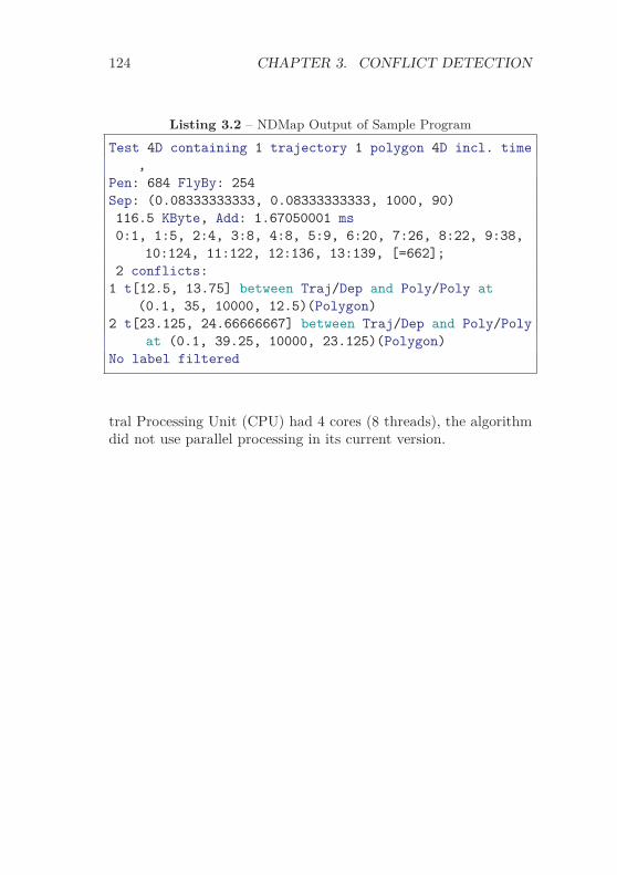
124 CHAPTER 3. CONFLICT DETECTION
Listing 3.2 – NDMap Output of Sample Program
Test 4D containing 1 trajectory 1 polygon 4D incl. time,
Pen: 684 FlyBy: 254Sep: (0.08333333333, 0.08333333333, 1000, 90)116.5 KByte, Add: 1.67050001 ms0:1, 1:5, 2:4, 3:8, 4:8, 5:9, 6:20, 7:26, 8:22, 9:38,
10:124, 11:122, 12:136, 13:139, [=662];2 conflicts:
1 t[12.5, 13.75] between Traj/Dep and Poly/Poly at(0.1, 35, 10000, 12.5)(Polygon)
2 t[23.125, 24.66666667] between Traj/Dep and Poly/Polyat (0.1, 39.25, 10000, 23.125)(Polygon)
No label filtered
tral Processing Unit (CPU) had 4 cores (8 threads), the algorithmdid not use parallel processing in its current version.

Chapter 4Conflict Detection in4D-Airspace
This chapter describes how the conflict detection algorithm ex-plained in chapter 3 can be used for conflict probe of 4D-trajectoriesin aviation. First of all, the algorithm needs to be configured cor-rectly. Therefore, the number of dimensions N is set to 4 and timereference mode is activated. Table 4.1 shows the setup for eachdimension covering one day of world-wide air traffic. S defines themandatory separation for each dimension. D is the resulting depthfor each dimension.
Table 4.1 – Setup of Conflict Map for 4D-Airspace
Dim. Unit Min Max S D∗
x/Longitude Deg -180 180 5/60 12.08y/Latitude Deg -90 90 5/60 11.08z/Altitude ft −1000 100 000 1000 6.66t/Time s 0 86 400 90 9.91∗ with D=log2
( max − minS
)
125

126 CHAPTER 4. CD IN 4D-AIRSPACE
4.1 Topological Isomorphism of Earth
4.1.1 The Earth-Mode
The last but one column of table 4.1 holds the mandatory separation�S. The value 5/60 is supposed to be the equivalent of 5 NM forlongitudes and latitudes. Due to Earth’s sphere-like shape, this isnot true for longitudes. One nautical mile is about one minute ofarc measured along latitude, or about one minute of arc of longitudeat the equator (fig. 4.1). All longitudinal minutes aside the equatormeasure less than 1 NM. Therefore, 5/60° is about 5 NM on theequator, but less aside.
15°
Figure 4.1 – Latitudes and Longitudes on Earth
If a tile is smaller than the mandatory separation �S conflictsmay be overlooked. The real distance between longitudinal arcs isillustrated best by the sinusoidal projection (fig. 2.25 on page 78).

4.1. TOPOLOGICAL ISOMORPHISM OF EARTH 127
Obviously, the distance between 5 longitudinal minutes at the polesis zero and therefore lower than any longitudinal separation Sλ.
Latit
ude
Longitude
5NM5NM
Figure 4.2 – Spherical and Corresponding Cartesian Model
When representing Earth in a Cartesian coordinate system, itis preferable to have an overlapping model (i. e., an aircraft flyingclose to a border between two tiles penetrates both tiles) instead ofhaving an uncovered gap between two tiles.
In order to respect the non-parallelism of longitudes the tilingalgorithm provides an Earth-mode. In Earth-mode the conflictdetection algorithm uses longitudes λ directly as x coordinates,see fig. 4.2. However, the non-parallelism of longitudes is takeninto account by adapting the longitudinal separation Sλ to theappropriate latitude ϕ:
S′λ(ϕ) =
Sλ
cos ϕ(4.1)
When precision needs to be very high and a spherical Earth modelis not accurate enough, the elliptical Mercator projection leads to(Osborne, 2008):
S′λ(ϕ) =
Sλ · (1 − e2 sin2 ϕ
)cos ϕ
(4.2)

128 CHAPTER 4. CD IN 4D-AIRSPACE
e2 = 2f − f2 = 0.00667053982 is the eccentricity of Earthwith f = 0.0033408505 being the flattening of Earth
Both eq. (4.1) and eq. (4.2) are not defined at the poles for ϕ = ±90°.Coming close to the Poles, objects occupy all longitudes.
Since e2 sin2 ϕ is close to zero, elliptical effects are very smalland often negligible in favor of faster calculations. For the sphericalformula, the longitudinal minutes matching 5 NM double at a lati-tude of 60°, since S′
λ(60°) = Sλ/0.5. For more complex objects, itis not necessary to recalculate cos ϕ each time. For not too big ob-jects, a common ϕ can be used, based on a conservative estimationchoosing the latitude of the object point being farthest from theequator. This can be calculated easily by analysis of the object’sbounding box.
Even though the decision is not critical in terms of overallcorrectness, the subdivision process also needs to be adapted inEarth mode. Since tiles are rectangular, but the longitudinal rangechanges with latitude, we need to specify which longitudinal rangeis taken for the subdivision decision. Starting with the whole Earthas root tile, longitudinal range at both minimum (Antarctic) andmaximum (Arctic) latitude is zero and thus not a good choice. Themaximum (full) longitudinal range is reached in the center of thelatitude interval. Concerning the longitudinal subdivision, a tileA(amin, amax) is generated as long as
(amax,λ − amin,λ) ≥ S′λ
(amax,ϕ + amin,ϕ
2
)(4.3)
Due to the tree structure and above formulated tiling decision,the tiling is not perfect at the Poles. Regarding the distance criteriaone tile is enough very close to the Poles, but the tree structuresubdivides longitudes in every depth step as long as it is beneficialfor the central latitude of a tile. Thus, several Pole tiles are usuallygenerated with an overlapping area of influence.

4.1. TOPOLOGICAL ISOMORPHISM OF EARTH 129
4.1.2 Great Circle Connections
As described in section 2.6.1, shortest surface connections on aspherical Earth model are great circles. Disregarding wind influence,it is most efficient for aircraft to fly along great circles. However, thetiling algorithm is based on a Cartesian coordinate system whereshortest connections between points are straight lines. Dependingon distance and direction, great circle distance and route differsignificantly from the Cartesian direct connection (fig. 4.3).
Maximum Deviation
Figure 4.3 – Cartesian vs. Great Circle Connection
Realizing great circles in the tiling algorithm is no problemtechnically. However, it would increase computation times sincegreat circle intersection is far more complex than axes-alignedCartesian intersection calculation.
The difference between Cartesian and great circle connectiongets smaller with more sampling points. Thus, conflict detectionworks precise enough with a sufficient number of sampling points.If the trajectory provider is unable to deliver denser points, theimplemented object class provides functionality interpolating newpoints based on great circle and WGS84 calculation before per-forming conflict probe. Figure 4.4 shows how the distance betweengreat circle and Cartesian connection depends on length of flightand its latitude, departure and arrival positions both having same
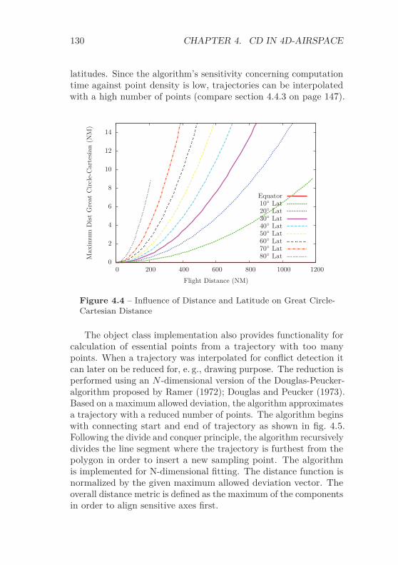
130 CHAPTER 4. CD IN 4D-AIRSPACE
latitudes. Since the algorithm’s sensitivity concerning computationtime against point density is low, trajectories can be interpolatedwith a high number of points (compare section 4.4.3 on page 147).
0
2
4
6
8
10
12
14
0 200 400 600 800 1000 1200
Max
imum
Dis
tG
reat
Cir
cle-
Car
tesi
an(N
M)
Flight Distance (NM)
Equator10◦ Lat20◦ Lat30◦ Lat40◦ Lat50◦ Lat60◦ Lat70◦ Lat80◦ Lat
Figure 4.4 – Influence of Distance and Latitude on Great Circle-Cartesian Distance
The object class implementation also provides functionality forcalculation of essential points from a trajectory with too manypoints. When a trajectory was interpolated for conflict detection itcan later on be reduced for, e. g., drawing purpose. The reduction isperformed using an N -dimensional version of the Douglas-Peucker-algorithm proposed by Ramer (1972); Douglas and Peucker (1973).Based on a maximum allowed deviation, the algorithm approximatesa trajectory with a reduced number of points. The algorithm beginswith connecting start and end of trajectory as shown in fig. 4.5.Following the divide and conquer principle, the algorithm recursivelydivides the line segment where the trajectory is furthest from thepolygon in order to insert a new sampling point. The algorithmis implemented for N-dimensional fitting. The distance function isnormalized by the given maximum allowed deviation vector. Theoverall distance metric is defined as the maximum of the componentsin order to align sensitive axes first.

4.1. TOPOLOGICAL ISOMORPHISM OF EARTH 131
1.2.3.
4.
5.
Figure 4.5 – Douglas-Peucker for Polygonal Approximation
4.1.3 Singularity and Discontinuity of Longi-tudes
Earth’s longitude is singular at the Poles and has a discontinuityat the ±180° meridian. Positions at Poles, i. e., latitude ϕ = ±90°,have an undefined longitude. Furthermore, the latitude/longitudegrid is highly non-linear close to the Poles. However, the Polesingularity is solved using the Cartesian ENU coordinate systemshown in fig. 4.2. When checking conflicts with tiles the singularityof eqs. (4.1) to (4.2) needs to be taken into account. Close to Poleobjects can be defined to be within all longitudinal Pole tiles, ifthere exist more than one. In worst case this results in a potentiallyconflicting object having no real conflict.
The discontinuity at the ±180° meridian (also known as inter-national date line) is more difficult to respect in an adequate way.The most efficient way of handling the discontinuity is avoidingit. Thus, if the air traffic scenario under investigation is limited toEurope, flights typically do not cross the date line. Working on ascenario with traffic between the United States and Asia is possibleby using a longitudinal interval of [0, 360] instead of [−180, 180]as long as the prime meridian through Greenwich is not crossed.That way, each scenario not touching one selected meridian canbe aligned by a suitable longitudinal interval avoiding the problem

132 CHAPTER 4. CD IN 4D-AIRSPACE
of discontinuity. However, if no such untouched meridian can beidentified, another solution is necessary.
On a spherical Earth model, longitudinal meridians -180° and180° (generally (k · 360° − 180°), k ∈ Z) are identical. The Cartesianrepresentation (fig. 4.2 on page 127) puts the endpoints of theinterval to the left and right border respectively, producing themaximum possible distance for identical longitudes. While a greatcircle connection on the spherical model is defined to be the shortestconnection between both points, the Cartesian representation onlyprovides one direct connection within the interval. Aiming for theshortest connection shortcuts via the longitudinal discontinuityneed to be taken into account. The green and red connections infig. 4.6 show the short and long great circle routes from P1 to P2in spherical and Cartesian representation.
Date Line
Date Line
P1 P2 P1
P2
Figure 4.6 – Shortest Connection on Spherical and CartesianRepresentation
The major issue with the connections crossing the date line isnot respecting it in a proper way, but finding an efficient solutionwithout downgrading the overall performance. The implementationrespects the wrap-around for the longitudinal dimension in Earth-mode. Additional sampling points are automatically inserted fortrajectories having the shortest connection via the longitudinaldiscontinuity λX . In total, four points are inserted around λX :

4.1. TOPOLOGICAL ISOMORPHISM OF EARTH 133
• The first point p1 is inserted just before passing the disconti-nuity. The point is located at amax,λ − ε for increasing andamin,λ + ε for decreasing longitudes.
• The second point p2 has same coordinates as p1, but a markedaltitude that is not within the scenario’s altitude interval.
• The third point p3 has same coordinates as p4 with the same(marked) altitude as p2.
• The fourth point p4 is inserted just after passing the disconti-nuity. The point is located at amin,λ + ε for increasing andamax,λ − ε for decreasing longitudes.
The marked points p2 and p3 are inserted in order to guarantee thatthe large Cartesian connection p2p3 is not considered for conflictdetection without retarding the code (dotted horizontal line infig. 4.7). Invalid conflicts on the vertical segments p1p2 and p3p4are very unlikely and can be omitted directly after conflict detection.An example is given in section 6.5. This procedure solves all issuesconcerning the detection of trajectories penetrating a tile. However,a conflict between two aircraft flying parallel on opposite sides ofλX still stays undetected.
Eastern Hemisphere Western Hemisphere Western Hemisphere Western Hemisphere
p1 p4
Start
Destination
p2p3
Date Line
Date Line
p3 p2
Figure 4.7 – Passing the Date Line in Cartesian Coordinates
Therefore, the fly-by detection also needs to be adapted. Thedilatation procedure defined in section 3.3.3 does not respect apossible longitude discontinuity. Dilatation of a tile at the disconti-nuity boundary does not produce one single but two unconnected

134 CHAPTER 4. CD IN 4D-AIRSPACE
N -dimensional spaces. As explained in section 3.3.4 on page 97fly-by objects only need to be taken into account when passing onthe positive (i. e., right) side. Since the likelihood of an aircraftbeing less than 5 NM right of the longitudinal discontinuity is low,objects are checked on insertion if they are relevant as discontinuityfly-by. Thus, the extra fly-by volume is checked only for few relevantobjects.
4.1.4 Alternative Earth Mapping
Pole and discontinuity issues raise the question if there are othermore suitable mappings from 4D-airspace into a 4-dimensionalCartesian coordinate system.
4.1.4.1 Spherical Coordinate System
A mapping avoiding pole and discontinuity issues is the sphericalcoordinate system depicted in fig. 4.8. Every point on (and in)Earth has unique 3D-coordinates. Airspace surrounds Earth andcan be addressed the same way.
X-Axis
Y-Axis
Z-Axis
Earth
Figure 4.8 – Alternate Earth Mapping

4.1. TOPOLOGICAL ISOMORPHISM OF EARTH 135
Containing no air traffic at all, the Earth volume is free ofconflicts and thus will only be subdivided at the Earth surface bythe conflict detection algorithm. Due to a large Earth radius of∼6 370 km and a small airspace height of typically less than 20 km,the conflict detection algorithm needs to focus on a small but widelyspread part of the initial volume. Even though this results in adeep tree (degrading also the performance), the tiling algorithmis predestined for these conditions. The reason why the sphericalcoordinate system was not used in this work is the alignment ofconflict metrics.
Using spherical coordinates, conflict dimensions are not alignedto the coordinate system anymore. Thus, altitude separation needsto be calculated by building the difference between Pythagoreandistances of both trajectories to Earth center. Distances concerninglatitude and longitude are even more complex to distinguish. Whilesmall tiles at the North Pole have z as altitude and x, y for longitudeand latitude, z is the latitude at the Equator. The unaligned axesalso complicate fly-by detection. In addition, the user interfacewould need to map between usual latitude/longitude/altitude rep-resentation and internal x, y, z coordinates introducing workloadand accuracy degradation.
Another problem with spherical mapping is the support of sparsetrajectories. Long distance trajectories with few sampling pointsrely on a proper interpolation. While linear interpolation is accept-able for the mapping described in section 4.1.1, it is problematicwith spherical coordinates. The direct connection between twospherical points of same distance to center gets closer to the cen-ter. If the center angle between the two points is big enough, thedirect connection will penetrate the Earth volume. In extreme, theconnection between two opposite points goes through the Earthcenter. Thus, linear interpolation varies altitude between two pointshaving same altitude. Since altitude is more sensitive than lateralseparation (1000 ft versus 5 NM), very dense trajectory points arenecessary to stay accurate enough, or the interpolation methodneeds to be changed to a more complex one.
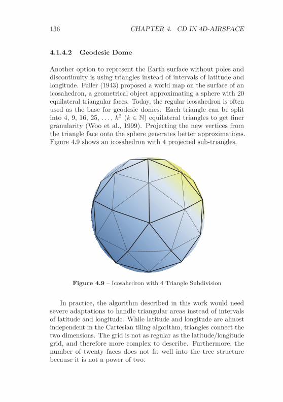
136 CHAPTER 4. CD IN 4D-AIRSPACE
4.1.4.2 Geodesic Dome
Another option to represent the Earth surface without poles anddiscontinuity is using triangles instead of intervals of latitude andlongitude. Fuller (1943) proposed a world map on the surface of anicosahedron, a geometrical object approximating a sphere with 20equilateral triangular faces. Today, the regular icosahedron is oftenused as the base for geodesic domes. Each triangle can be splitinto 4, 9, 16, 25, . . . , k2 (k ∈ N) equilateral triangles to get finergranularity (Woo et al., 1999). Projecting the new vertices fromthe triangle face onto the sphere generates better approximations.Figure 4.9 shows an icosahedron with 4 projected sub-triangles.
Figure 4.9 – Icosahedron with 4 Triangle Subdivision
In practice, the algorithm described in this work would needsevere adaptations to handle triangular areas instead of intervalsof latitude and longitude. While latitude and longitude are almostindependent in the Cartesian tiling algorithm, triangles connect thetwo dimensions. The grid is not as regular as the latitude/longitudegrid, and therefore more complex to describe. Furthermore, thenumber of twenty faces does not fit well into the tree structurebecause it is not a power of two.

4.2. TRAFFIC SAMPLES AND CONDITIONS 137
Integration of the triangular layout in the generic NDMap breaksthe general approach, and a separate approach would be preferable.Furthermore, since triangle borders are not axis-aligned, degradationin computation speed is anticipated. All in all, the higher structuralcomplexity is not a good trade-off for the absence of poles anddiscontinuities.
4.2 Traffic Samples and Conditions
In the remaining work, conflict detection and resolution is basicallyperformed on two scenarios described in this section, one scenariocovering one day of German traffic, and one scenario holding Euro-pean traffic.
4.2.1 German Traffic Sample
Germany has one of World’s densest net of airfields and airports(∼550 (Central Intelligence Agency, 2007)). The German air navi-gation service provider DFS Deutsche Flugsicherung GmbH (DFS)controlled 3.06 million flights in 2011 (DFS Deutsche Flugsicherung,2011). The German traffic sample is based on one of the busiestdays 2008 holding 10 256 flights. Using flight plans and radar tracks,trajectories were generated with the AFMS to get a traffic samplewith realistic assumptions. However, since aircraft comply with theperformance models and weight assumptions from the AFMS, theresulting sample is by no means identical to the real traffic day,and thus contains ∼3 k conflicts based on a conflict definition of5 NM/1000 ft in and above 5000 ft and 3 NM/1000 ft below.
Trajectories are not complete from departure to destination butcut close to the country borders in order to cover only the Germanpart of flight (fig. 4.11). Figure 4.10 shows the distribution offlights along daytime. Peak traffic level is ∼500 concurrent flights.The sample contains flights departing from, arriving in, and flyingthrough Germany. Some callsigns are used twice on the sameday; the second flight replaces the first one in conflict detection onoccurrence. Further information on the German traffic sample is

138 CHAPTER 4. CD IN 4D-AIRSPACE
0
100
200
300
400
500
600
00:00 04:00 08:00 12:00 16:00 20:00 00:00
Num
ber
ofA
irbo
rne
Flig
hts
Time of Day
Figure 4.10 – Airborne Aircraft in German Traffic Sample
gathered in table 4.2. The untypical high maximum flight durationsand distances are provoked by some experimental flights also beingpart of the traffic sample. These particular aircraft were obviouslynot accomplishing a transport task but performed special missionsproducing abnormal data.
Figure 4.11 – GermanAir Traffic Sample
Figure 4.12 – Optimized Euro-pean Air Traffic Sample

4.2. TRAFFIC SAMPLES AND CONDITIONS 139
0
500
1000
1500
2000
2500
3000
3500
4000
00:00 04:00 08:00 12:00 16:00 20:00 00:00
Num
ber
ofA
irbo
rne
Flig
hts
Time of Day
Figure 4.13 – Airborne Aircraft in European Traffic Sample
4.2.2 European Traffic Sample
The European traffic sample holds 33 069 airborne movements. Incontrast to the German sample, flights are not cut at Europeanborders, but are usually complete from departure to destination.The data is taken from the Demand Data Repository (DDR) pro-vided by Eurocontrol (2010). The sample contains flights departingfrom, arriving in, and flying through Europe. As in the Germansample, some callsigns were used multiple times a day. However,since the callsign is used as identifier in the NDMap the callsignswere unified by appending numbers in order to investigate the fulltraffic. As fig. 4.13 shows, the sample starts with departures at mid-night, and holds all aircraft flying into the next day. The peak levelof ∼3700 aircraft being airborne at the same time is significantlyhigher compared to Germany because:
• The scenario contains more than 3 times more movements;and

140 CHAPTER 4. CD IN 4D-AIRSPACE
• Flights are complete from take-off to touchdown. An aircraftdeparting from the United States flying into Europe later onis counted for the whole flight duration.
The European traffic sample was modified to create an optimizedscenario. In order to fly as efficient as possible, flights were put tomost direct routes and optimum altitude and speed profiles. Sincethe aircraft do not respect today’s airway structure the samplerepresents a future scenario.
The only data taken from the original sample is:
Callsign as an identifier for each flight.
Aircraft type describing the performance of specific aircraft
Departure and arrival runways defining the route to be flown
Departure time as the time reference for the flight
Cruise flight level defining the maximum altitude of flight.
All flights are optimized by applying the direct great circleconnection from departure to arrival airport. Since the originalrunways are used, up to two waypoints are inserted at each airport incase angles get too pointed (Kuenz and Schwoch, 2012). Figure 4.14shows an example where four additional points (D1 and D2 forthe departure and A1 and A2 for the arrival) are necessary to geta feasible route layout. The new constraints for the trajectorypredictor (compare section 2.3) were gathered by Gunnar Schwoch(DLR) in the context of the 4 Dimensional-Contracts - Guidance andControl (4DCo-GC) project under the European Union’s SeventhFramework Programme for Research (FP7).
Based on aforementioned inputs, new optimized trajectoriesare generated using the AFMS described in section 2.3.1. Besideshaving much more efficient trajectories, the main difference to thereal life traffic without conflicts is a significantly increased numberof conflicts. The use of flexible route structures changes flightdurations significantly by flying shorter great circle routes andaircraft-optimized speeds. This results in uncoordinated en-routeand arrival segments and an overall conflict count of nearly 29 000.

4.3. RESULTS FROM CONFLICT DETECTION 141
D1
D2 A1
A2
5 NM
5 NM
Figure 4.14 – Four Points in Worst Case for a Flyable RouteLayout
Further information on the European traffic sample is collected intable 4.2.
4.3 Results from Conflict Detection
Detection of conflicts becomes complex with a large number ofobjects. Figure 4.15 shows conflict detection times for the Ger-man sample using the basic algorithm described in section 2.4.2.Comparing each trajectory against each other results in conflictdetection times of more than 3.5 days for ∼10 k trajectories1. Dueto the quadratic complexity O(N2) using even bigger scenarios isunwise with this algorithm. Figure 4.16 depicts the results of theoptimized version of the algorithm described in section 2.4.2. Theoverall detection time is reduced to less than 5.5 hours by checkingconflicts only for aircraft being airborne simultaneously.
Even though the worst case complexity is still quadratic (e. g., ifall aircraft are airborne at the same time), the conflict detection timehas a nearly linear relation to the number of flights at least for thegiven scenario complexity. However, the overall poor performance of∼1.8 s detection time per trajectory restricts the variety of possibleapplication areas.
1Be aware of the y-axis scaling being non-consistent in this section due tovery different computation times.
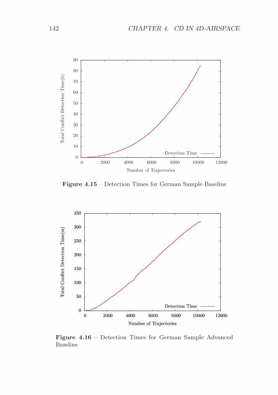
142 CHAPTER 4. CD IN 4D-AIRSPACE
0
10
20
30
40
50
60
70
80
90
0 2000 4000 6000 8000 10000 12000
Tota
lCon
flict
Det
ecti
onT
ime(
h)
Number of Trajectories
Detection Time
Figure 4.15 – Detection Times for German Sample Baseline
0
50
100
150
200
250
300
350
0 2000 4000 6000 8000 10000 12000
Tota
lCon
flict
Det
ecti
onT
ime(
m)
Number of Trajectories
0
50
100
150
200
250
300
350
0 2000 4000 6000 8000 10000 12000
Tota
lCon
flict
Det
ecti
onT
ime(
m)
Number of Trajectories
Detection TimeDetection Time
Figure 4.16 – Detection Times for German Sample AdvancedBaseline

4.3. RESULTS FROM CONFLICT DETECTION 143
Table 4.2 – Properties of Traffic Samples
German EuropeanAircraft [#] 10 256 33 069Uniques [#] 9783 33 069Extension Cut-to-border CompleteConflicts [#] 3051 28 986
Heavy [%] 12.5 % 9.6 %Medium [%] 83.8 % 83.8 %Light [%] 3.7 % 6.6 %
Duration (μ ± σ) 0:46:04 ± 0:19:11 2:01:45 ± 2:10:11[H:MM:SS] Interval [0:35, 7:43:38] [7:45, 17:59:57]
Distance (μ ± σ) 287.6 ± 118.4 820.9 ± 1021.8[NM] Interval [1.9, 2615.3] [19.5, 8310]
Points (μ ± σ) 47.1 ± 18.9 89.1 ± 61.0[#] Interval [2, 454] [6, 1019]
Latitude (μ ± σ) 50.3 ± 2.0 45.6 ± 10.3[deg] Interval [46.5, 55.2] [-35.0, 88.1]
Longitude (μ ± σ) 10.1 ± 2.6 8.0 ± 28.2[deg] Interval [5.5, 15.9] [-123.2, 140.4]
Altitude (μ ± σ) 24 914 ± 12 225 19 715 ± 14 042[ft] Interval [0, 45 000] [-72, 47 000]
Time (μ ± σ) 12:37:24 ± 5:10:57 13:49:40 ± 3:54:02[H:MM:SS] Interval [-2:21:01, 23:59:57] [-51:57, 39:05:36]
The tiling algorithm described in this document reduces detec-tion times significantly. Figure 4.17 depicts the performance of the4-dimensional tiling algorithm. The detection of all conflicts is per-formed in ∼18.5 s for the German traffic sample. Thus, the averagedetection time per trajectory is as low as 1.8 ms. Figure 4.17 alsoshows the allocated memory of the hexadecimal tree. Using about58 KiB per trajectory the algorithm can handle much more than theGerman area on standard off-the-shelf personal computer hardware.Both computation time and memory usage are mostly linear for

144 CHAPTER 4. CD IN 4D-AIRSPACE
the given scenario complexity. The computational performance canbe tuned to 1.61 ms per trajectory by adapting the minimum tileduration (fig. 4.24 on page 153). However, this increases the averagememory usage to 68 KiB per trajectory.
0
2
4
6
8
10
12
14
16
18
20
0 2000 4000 6000 8000 10000 120000
0.1
0.2
0.3
0.4
0.5
0.6
Tota
lCon
flict
Det
ecti
onT
ime(
s)
Mem
ory
Usa
ge(G
B)
Number of Trajectories
Detection TimeMemory Usage
Figure 4.17 – Detection Times for German Sample with TilingAlgorithm
Figure 4.18 depicts the results from the tiling algorithm for theEuropean sample. The prediction time is nearly linear with anaverage of 5.3 ms per trajectory. The steeper part in the center andthe more shallow start and end are likely caused by the time basedsorting of the scenario. Traffic density is lower around midnightand higher during daytime, compare fig. 4.13. The computationalperformance can be tuned to 4.97 ms per trajectory by optimizingthe minimum tile duration (fig. 4.25 on page 153).
Trying to find a reason for the rather big difference in calculationtimes to the German sample (5.3 ms vs. 1.8 ms) is a complex job.Performance indicators are discussed in section 4.4.

4.4. PERFORMANCE INDICATORS 145
0
20
40
60
80
100
120
140
160
180
0 5 10 15 20 25 30 350
0.5
1
1.5
2
2.5
3
3.5
4To
talC
onfli
ctD
etec
tion
Tim
e(s)
Mem
ory
Usa
ge(G
B)
Number of Trajectories in Thousand
Detection TimeMemory Usage
Figure 4.18 – Detection Times for European Sample with TilingAlgorithm
4.4 Performance Indicators
Worst case performance of the provided algorithm is O(N2) inparticular for the case that all N trajectories are identical. Buildingthe tree would not occlude any trajectory pairs from conflict probe.Thus, every single trajectory needs to be checked against each other,as also done by the baseline algorithm. However, as can be readfrom the promising results, in practice the algorithm performs verywell.
The main influencing factors on the algorithm’s run-time arediscussed in following sections.
4.4.1 Number of Trajectories
Since the conflict probing is done sequentially the number of trajec-tories has influence on the total run-time. Talking about calculationtimes per trajectory, the number of trajectories has only weak in-fluence. If the trajectories are well distributed in the 4D-airspace,

146 CHAPTER 4. CD IN 4D-AIRSPACE
calculation times are low even for a high number of trajectories. Iftrajectories are identical, computation of conflicts is complex forfew trajectories already.
The only weak dependence of trajectory count from calculationtimes per trajectory is proven by performing conflict detection ona quadrupled German traffic sample. Initially, the German trafficsample does not leave the Northern and Eastern hemisphere. Thequadrupled German traffic sample is generated by first mirroringtraffic at the zero meridian, and mirroring the resulting traffic at theequator. This leaves densities and length of trajectories constant,but quadruples the total trajectory count. As shown in fig. 4.19,the memory is four times higher than the memory used for theGerman traffic sample. In contrast, the computation time pertrajectory nearly stays the same with ∼2.3 ms per trajectory. Theadditional ∼0.5 ms per trajectory may be a result from the largerarrays for trajectories and conflicts, e. g., when verifying if a conflicthas already been identified before.
0
10
20
30
40
50
60
70
80
90
100
0 5 10 15 20 25 30 35 400
0.5
1
1.5
2
2.5
Tota
lCon
flict
Det
ecti
onT
ime(
s)
Mem
ory
Usa
ge(G
B)
Number of Trajectories in Thousand
Detection TimeMemory Usage
Figure 4.19 – Detection Times for Quadrupled German Scenario
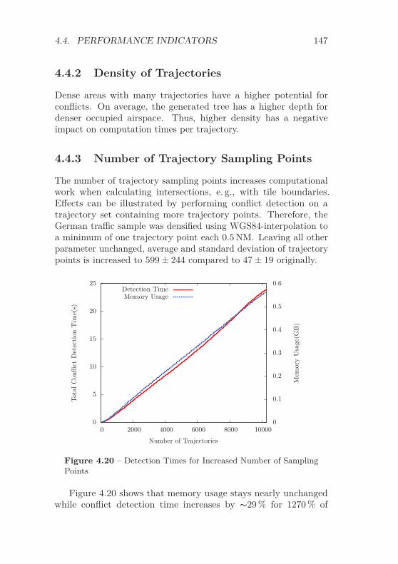
4.4. PERFORMANCE INDICATORS 147
4.4.2 Density of Trajectories
Dense areas with many trajectories have a higher potential forconflicts. On average, the generated tree has a higher depth fordenser occupied airspace. Thus, higher density has a negativeimpact on computation times per trajectory.
4.4.3 Number of Trajectory Sampling Points
The number of trajectory sampling points increases computationalwork when calculating intersections, e. g., with tile boundaries.Effects can be illustrated by performing conflict detection on atrajectory set containing more trajectory points. Therefore, theGerman traffic sample was densified using WGS84-interpolation toa minimum of one trajectory point each 0.5 NM. Leaving all otherparameter unchanged, average and standard deviation of trajectorypoints is increased to 599 ± 244 compared to 47 ± 19 originally.
0
5
10
15
20
25
0 2000 4000 6000 8000 100000
0.1
0.2
0.3
0.4
0.5
0.6
Tota
lCon
flict
Det
ecti
onT
ime(
s)
Mem
ory
Usa
ge(G
B)
Number of Trajectories
Detection TimeMemory Usage
Figure 4.20 – Detection Times for Increased Number of SamplingPoints
Figure 4.20 shows that memory usage stays nearly unchangedwhile conflict detection time increases by ∼29 % for 1270 % of

148 CHAPTER 4. CD IN 4D-AIRSPACE
the initial sampling points. Thus, the link between number ofsampling points and calculation times is not very strong. Thefact that memory usage even decreases slightly can be explainedby the WGS84-interpolation while the NDMap performs linearinterpolation internally.
4.4.4 Length of Trajectories
The trajectory length has significant influence on computation timesbecause long trajectories affect many tiles. Thus, a doubled lengthof a trajectory is comparable to two single length trajectories interms of computational burden.
4.4.5 Number of Potential and Real Conflicts
Obviously, a high number of conflicts in a scenario increases com-putational work. The average depth of the hexadecimal tree getshigher, and number of final conflict detection probes increases.
4.4.6 Summary of Performance Indicators
Finally, coming back to the difference of computation times betweenGerman and European sample, scenario density is probably not thereason because 10 000 trajectories in Germany is a higher averageload than 33 000 trajectories over whole Europe. Main reasons forthe worse performance of the European sample are likely the nearly3 times longer trajectories and the higher number of sampling points.Also the allocated memory is high compared to the German sample.About 106 KiB of memory was used per trajectory.
4.5 Performance Optimization for Con-flict Detection
This section discusses the choice of minimum tile sizes in order toguarantee a mandatory separation �S. As described in section 3.3.10

4.5. PERFORMANCE OPTIMIZATION FOR CD 149
on page 104 the minimum tile size needs to be at least as big as theminimum separation �S in order to detect all conflicts, but mightalso be bigger. Therefore, detection runs were performed withdifferent configurations of the hexadecimal tree to find the optimumset of parameters. In this section, all runs were performed usingthe German traffic sample.
4.5.1 Lateral Tile Size Optimization
Starting with the lateral tile size, fig. 4.21 shows detection timesand memory allocation for lateral separation distances from 5 NMto 20 NM. The detection time increases apart from some jittermonotonically with larger lateral tiles. The memory usage decreasesslightly with increasing lateral size of tiles. The figure also showsthe average number of penetrations and fly-bys per tile. Especiallyan increasing number of fly-bys per tile is noticeable. As depictedon fig. 3.8 on page 96, fly-by zones get larger with increasing lateralseparation size. The number of penetrations stays constant. Thereduction of tree depth counteracts the increasing number of fly-bys,resulting in an overall decreasing memory usage. Summarizing, itis beneficial for run-time to set the minimal lateral tile size to thelateral conflict size. Using larger tiles for the leaves reduces thenecessary memory slightly, but also increases calculation times.
4.5.2 Vertical Tile Size Optimization
The results look different when changing vertical tile size instead oflateral size as plotted in fig. 4.22. While memory usage decreasesslightly for increasing vertical size, detection times increase. Moreeye-catching are three steps where memory usage and calculationtime decrease simultaneously. This behavior can be explained byhaving a closer look at table 4.1. The altitude dimension needs thelowest number of subdivisions (6.66) to get down to minimum tilesize. By increasing the smallest vertical tile size, the number ofnecessary subdivisions is further decreased. Table 4.3 shows thenecessary number of subdivisions for increased Vertical Tile Size

150 CHAPTER 4. CD IN 4D-AIRSPACE
16
18
20
22
24
26
28
30
32
34
36
6 8 10 12 14 16 18 200.2
0.4
0.6
0.8
1
1.2
1.4
1.6
1.8
2
2.2
Tota
lCon
flict
Det
ecti
onT
ime(
s)
Mem
ory
Usa
ge(G
B)/
Affe
ctio
nspe
rT
ile
Smallest Tile Size (NM)
Detection TimeMemory Usage
Penetrations per TileFlyBys per Tile
Figure 4.21 – Variation of Tile Size
(VTS). Obviously, the steps in fig. 4.22 are placed where the numberof vertical subdivisions decreases by one.
Table 4.3 – Vertical Dimension with Increased Vertical Tile Size
Min Max VTS D∗
-1000 100 000 1000 6.66-1000 100 000 1578 6.00-1000 100 000 3156 5.00-1000 100 000 6312 4.00∗ with D=log2
( max − minVTS
)When the vertical subdivision downto minimum tile size is
finished in the tree, the whole tree starts getting thinner. Eachnode has a maximum of 8 instead of 16 children. This is beneficialfor memory and run-time. Summarizing, a starting value of 1000 ftis a good choice. Another efficient opportunity is using the nextpoint where the subdivision count decreases, namely 1578 ft orslightly above to be on the safe side. Using even higher minimum

4.5. PERFORMANCE OPTIMIZATION FOR CD 151
17
18
19
20
21
22
23
24
25
1000 2000 3000 4000 5000 6000 7000 8000 9000 100000
0.2
0.4
0.6
0.8
1
1.2
1.4
1.6
1.8To
talC
onfli
ctD
etec
tion
Tim
e(s)
Mem
ory
Usa
ge(G
B)/
Affe
ctio
nspe
rT
ile
Smallest Tile Altitude (ft)
Detection TimeMemory Usage
Penetrations per TileFlyBys per Tile
Figure 4.22 – Variation of Altitude
values is not beneficial for overall run-time. The approach of takingthe subdivision positions into account is respected by the modifiedbalancing algorithm in section 4.5.4.
4.5.3 Time-based Tile Size Optimization
The effects of varying the time-based tile size are shown in fig. 4.23.With a very fine granularity of one second, both memory usage andcomputation times are high. Too large tiles result in low memoryusage, but increased computation times. However, the initiallychosen 90 seconds representing a typical time-based separationbetween two succeeding aircraft with approach speeds are not thebest choice in terms of computation times. Table 4.4 shows thestep-creating increments of time depth. In order to increase thecalculation speed a minimum tile duration below 84.375 s should beselected. Figures 4.24 and 4.25 show the results for a tile duration of80 s for Germany and Europe respectively. Average detection timesare 1.61 ms for Germany and 4.97 ms for Europe per trajectory.

152 CHAPTER 4. CD IN 4D-AIRSPACE
Table 4.4 – Time Dimension with Increased Tile Duration
Min Max Duration D∗
0 86 400 90 9.910 86 400 84.375 10.000 86 400 168.75 9.000 86 400 337.5 8.000 86 400 675 7.00
∗ with D=log2( max − min
Duration
)
16
18
20
22
24
26
28
30
32
0 50 100 150 2000.4
0.6
0.8
1
1.2
1.4
1.6
1.8
2
Tota
lCon
flict
Det
ecti
onT
ime(
s)
Mem
ory
Usa
ge(G
B)/
Affe
ctio
nspe
rT
ile
Smallest Tile Time (s)
Detection TimeMemory Usage
Penetrations per TileFlyBys per Tile
Figure 4.23 – Variation of Time
4.5.4 Balancing the Tree
The results in this section are based on a minimum time durationof 80 s, as experienced in the last section.
As described in section 3.3.9, balancing of a tree adapts startingintervals of each dimension in a way that ensures reaching minimumtile size for all dimensions at the same level of depth. The resultsfrom an automatically balanced tree for the German traffic sampleare shown in fig. 4.26. While using about 25 percent more memory

4.5. PERFORMANCE OPTIMIZATION FOR CD 153
0
2
4
6
8
10
12
14
16
18
0 2000 4000 6000 8000 100000
0.1
0.2
0.3
0.4
0.5
0.6
0.7To
talC
onfli
ctD
etec
tion
Tim
e(s)
Mem
ory
Usa
ge(G
B)
Number of Trajectories
Detection TimeMemory Usage
Figure 4.24 – Results for 80 Seconds Tile Duration (Germany)
0
20
40
60
80
100
120
140
160
180
0 5000 10000 15000 20000 25000 300000
0.5
1
1.5
2
2.5
3
3.5
4
Tota
lCon
flict
Det
ecti
onT
ime(
s)
Mem
ory
Usa
ge(G
B)
Number of Trajectories
Detection TimeMemory Usage
Figure 4.25 – Results for 80 Seconds Tile Duration (Europe)
than the unbalanced version (compare fig. 4.17), calculation timeremains the same. Balancing on the European traffic sample also
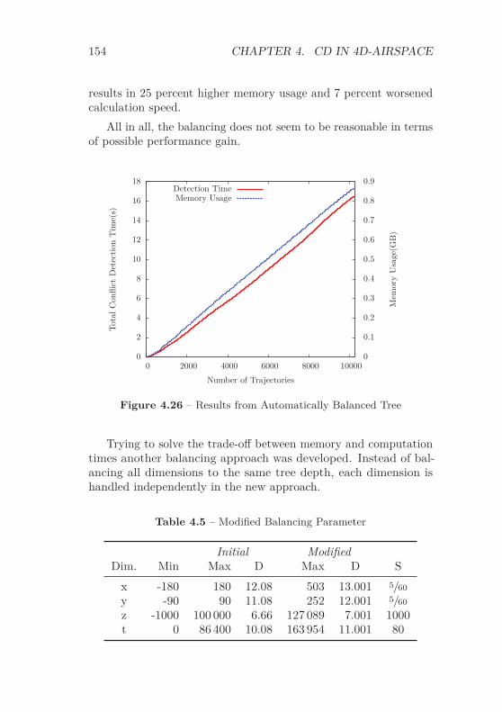
154 CHAPTER 4. CD IN 4D-AIRSPACE
results in 25 percent higher memory usage and 7 percent worsenedcalculation speed.
All in all, the balancing does not seem to be reasonable in termsof possible performance gain.
0
2
4
6
8
10
12
14
16
18
0 2000 4000 6000 8000 100000
0.1
0.2
0.3
0.4
0.5
0.6
0.7
0.8
0.9
Tota
lCon
flict
Det
ecti
onT
ime(
s)
Mem
ory
Usa
ge(G
B)
Number of Trajectories
Detection TimeMemory Usage
Figure 4.26 – Results from Automatically Balanced Tree
Trying to solve the trade-off between memory and computationtimes another balancing approach was developed. Instead of bal-ancing all dimensions to the same tree depth, each dimension ishandled independently in the new approach.
Table 4.5 – Modified Balancing Parameter
Initial ModifiedDim. Min Max D Max D S
x -180 180 12.08 503 13.001 5/60
y -90 90 11.08 252 12.001 5/60
z -1000 100 000 6.66 127 089 7.001 1000t 0 86 400 10.08 163 954 11.001 80
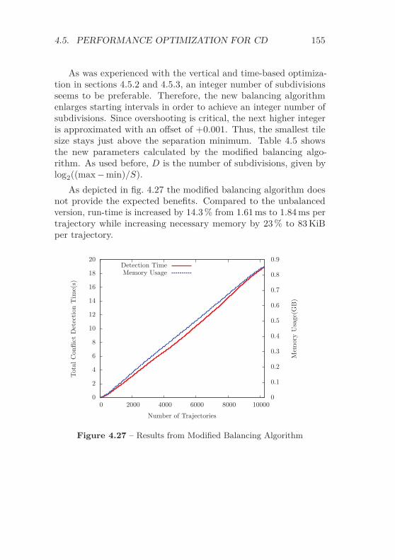
4.5. PERFORMANCE OPTIMIZATION FOR CD 155
As was experienced with the vertical and time-based optimiza-tion in sections 4.5.2 and 4.5.3, an integer number of subdivisionsseems to be preferable. Therefore, the new balancing algorithmenlarges starting intervals in order to achieve an integer number ofsubdivisions. Since overshooting is critical, the next higher integeris approximated with an offset of +0.001. Thus, the smallest tilesize stays just above the separation minimum. Table 4.5 showsthe new parameters calculated by the modified balancing algo-rithm. As used before, D is the number of subdivisions, given bylog2((max − min)/S).
As depicted in fig. 4.27 the modified balancing algorithm doesnot provide the expected benefits. Compared to the unbalancedversion, run-time is increased by 14.3 % from 1.61 ms to 1.84 ms pertrajectory while increasing necessary memory by 23 % to 83 KiBper trajectory.
0
2
4
6
8
10
12
14
16
18
20
0 2000 4000 6000 8000 100000
0.1
0.2
0.3
0.4
0.5
0.6
0.7
0.8
0.9
Tota
lCon
flict
Det
ecti
onT
ime(
s)
Mem
ory
Usa
ge(G
B)
Number of Trajectories
Detection TimeMemory Usage
Figure 4.27 – Results from Modified Balancing Algorithm

156 CHAPTER 4. CD IN 4D-AIRSPACE
4.5.5 Focus on Aircraft
As described in section 3.6, run-time and memory usage can bedrastically improved when the collision detection focuses on a subsetof trajectories. An exemplary application is the responsibility of anair traffic controller for a predefined subset of aircraft as describedin section 4.7.2.
Figure 4.28 depicts results for trial runs with 1-200 selectedaircraft based on the German traffic sample. Aircraft are selectedby random from the traffic sample and registered in the NDMapbefore loading the scenario. The random selection of aircraft im-pedes a monotonic increase of total detection time. Selecting onlyone aircraft, generation of the whole tree takes 1.1 seconds whileusing 401 KiB memory. Focusing on six aircraft as done in theLuftraummanagment 2020 (LRM2020) project, the tree generationincluding conflict detection for the selected 6 flights takes 1.5 s.
1
1.5
2
2.5
3
3.5
4
4.5
5
5.5
0 50 100 150 2000
10
20
30
40
50
60
Tota
lCon
flict
Det
ecti
onT
ime(
s)
Mem
ory
Usa
ge(M
B)
Number of Selected Trajectories
Detection TimeMemory Usage
Figure 4.28 – Algorithm’s Performance for Different Numbers ofSelected Aircraft
Selecting aircraft increases performance without creating a bigoverhead. The break-even point in terms of performance comparedto the standard setup is reached with ∼7600 selected aircraft, where

4.5. PERFORMANCE OPTIMIZATION FOR CD 157
the calculation takes ∼18 s and uses 583 MiB of memory. Thus, if afocus on a subset of aircraft can be set, this should be done unlessthe subset contains more than 7600 aircraft for the German trafficsample.
4.5.6 Shrinking the Root Tile
This section investigates if starting with large root tiles penalizesthe algorithm’s performance significantly. Selecting the whole worldas root tile for the German traffic sample with latitudes in [46.5°,55.2°] and longitudes in [5.5°, 15.9°] (table 4.2 on page 143) mayresult in an unnecessary long search path for conflicts.
Therefore, the conflict detection was executed with a shrunkroot tile with latitudes in [46.5°, 55.2°], longitudes in [5.5°, 15.9°]and altitudes in [-500 ft, 50 000 ft]. The unexpected results aredepicted in fig. 4.29. The shrunk root tile results claim 45 % morememory usage and a 37 % increase of calculation time. Turning onthe balancing algorithm produced even worse results.
0
5
10
15
20
25
0 2000 4000 6000 8000 100000
0.2
0.4
0.6
0.8
1
1.2
Tota
lCon
flict
Det
ecti
onT
ime(
s)
Mem
ory
Usa
ge(G
B)
Number of Trajectories
Detection TimeMemory Usage
Figure 4.29 – Results from Shrunk Root Tile

158 CHAPTER 4. CD IN 4D-AIRSPACE
Trying to explain the increase in memory usage and run-time,table 4.6 lists the number of generated tiles in each depth level forboth defined root tiles. As expected, the shrunk root tile needs lessdepth than the Earth root tile (10 versus 11), and the shrunk roottile generates a thicker tree close to the root (16 versus 4 nodes inlevel 1). In total, the shrinking increases the number of generatedtiles significantly by 45 %. Since the only values changed are thenumber of subdivisions for each single dimension, the reason needsto be the shift between the dimensions against each other. Onepossible explanation is that it might be beneficial to let the timedimension split before all other dimensions split occupied airspace.However, trials increasing all dimensions but time to magnify thateffect were not successful.
Table 4.6 – Number of Nodes - Earth vs. Shrunk
Earth-Root Shrunk-Root
0 1 11 4 162 8 2563 32 33884 116 39 8385 1754 364 2776 15 050 1 114 1107 65 182 617 1538 249 573 537 0199 602 255 445 24910 878 849 374 01111 593 092 N/A
Total 2 405 916 3 495 318
The observed behavior indicates that the algorithm is sensitiveagainst different starting conditions. It also illustrates that theproposed input balancing is not perfect – extending the shrunk tileto Earth dimensions obviously is a better option.
However, the conditions leading to the best calculation perfor-mance are nontrivial and for sure also not independent from the

4.6. COMPARISON WITH OCTREES 159
input data. Several trials with different starting intervals were per-formed with the result that the Earth intervals as initially chosenare close to optimum. Future work on that topic may result in aneven better input balancing algorithm.
4.6 Comparison with Octrees
Since the implementation of the NDMap is generic concerning thenumber of dimensions, detection runs can easily be performed withless than 4 dimensions. This section shows results from two 3D-octree configurations. In order to get the same final conflicts as inthe 4D version, the external conflict function still checks conflictsin all 4 dimensions.
Figure 4.30 presents the results using an octree holding latitude,longitude, and altitude as proposed by Hildum and Smith (comparesection 2.4.3 on page 63). Comparing the outcome with the 4D-configuration in fig. 4.24, the procedure needs only 12 % of memory,but uses a 36 times higher calculation time.
Generation of the data was a bit difficult. The final conflictdetection needs a 4-dimensional vector to validate the conflict.However, if time is not included in the tree, the corresponding4D-point cannot be identified clearly without ambiguity. Therefore,the NDMap was used in 4D mode. In order to avoid benefits fromthe time dimension, a minimum tile duration of 86 400 s (i. e., oneday) was applied.
Figure 4.31 shows results from another octree configuration ofthe NDMap holding latitude, longitude, and time. This time, theNDMap was configured in real 3D mode. Using about 364 MiB ofmemory, this configuration needs about 220 % of the time from thereference 4D-hexadecimal configuration in fig. 4.24. The relativegood performance indicates that two aircraft rarely cross above eachother at the same time. It also proves that the provided algorithmsperform well in 3 dimensions.
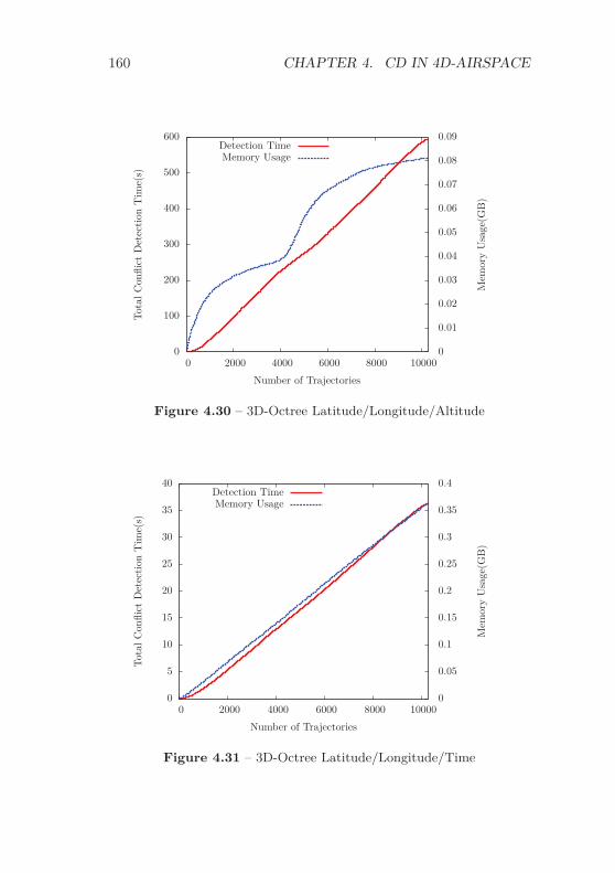
160 CHAPTER 4. CD IN 4D-AIRSPACE
0
100
200
300
400
500
600
0 2000 4000 6000 8000 100000
0.01
0.02
0.03
0.04
0.05
0.06
0.07
0.08
0.09To
talC
onfli
ctD
etec
tion
Tim
e(s)
Mem
ory
Usa
ge(G
B)
Number of Trajectories
Detection TimeMemory Usage
Figure 4.30 – 3D-Octree Latitude/Longitude/Altitude
0
5
10
15
20
25
30
35
40
0 2000 4000 6000 8000 100000
0.05
0.1
0.15
0.2
0.25
0.3
0.35
0.4
Tota
lCon
flict
Det
ecti
onT
ime(
s)
Mem
ory
Usa
ge(G
B)
Number of Trajectories
Detection TimeMemory Usage
Figure 4.31 – 3D-Octree Latitude/Longitude/Time

4.7. APPLICATION IN PROJECTS 161
4.7 Application in Projects
The software module NDMap has already been used by severalprojects at DLR. The applications differ in applied time horizons andtraffic complexity significantly. This section gives short descriptionsfor some of the projects and especially focuses on the applicationof the NDMap.
4.7.1 Future Air Ground Integration
The Future Air Ground Integration (FAGI) project has taken placefrom 2007 to 2009 and used a first version of the NDMap modulefor STCA and TBO (Kuenz and Edinger, 2010a,b). The projectfocused on providing a transition from today’s vector-based controlof aircraft into a TBO environment supporting both FMS equippedand unequipped aircraft.
The FAGI concept distinguishes aircraft by their equipage:
• Aircraft equipped with a 4D-FMS are capable to predict andfulfill 4D trajectories board-autonomously. The expectedaccuracy is ±6 s as one out of nine aircraft in European trafficwas capable in 2007 (Smedt and Berz, 2007).
• Conventional equipped aircraft without an onboard 4D-FMS are incapable of high precision board-autonomous 4D-guidance.
The key element of the proposed 4D concept for an advancedTerminal Maneuvering Area (TMA) handling is the late merging ofall arriving traffic. Before merging, arriving aircraft are separatedprocedurally by staggering them laterally in an Extended TMA(E-TMA) allowing each aircraft to fly its individual speed andaltitude profile. When entering the E-TMA, a time constraint forthe merging point is assigned to each aircraft. The late mergingpoint for all aircraft is located just before the final approach. Theearly assignment of time constraints enables arriving aircraft tofulfill the requested time in an efficient way, i. e., speed adaptation.Therefore, the E-TMA is rather big (80 NM to 120 NM radius). If

162 CHAPTER 4. CD IN 4D-AIRSPACE
speed variation is not enough to reach the constraint, strategic pathstretching can be used to delay aircraft further. Parallel routes fromevery entry point to the late merging point enables faster aircraftto overtake slower aircraft (fig. 4.32).
Aircraft not entering near a static E-TMA entry are guided bymeans of dynamic routing. Depending on the equipage, there aretwo different approaches possible:
• 4D-equipped aircraft are able to generate their own optimum4D-trajectory board-autonomously. They fulfill a groundpredicted time constraint at late merging with high precision,ideally without any interventions after the negotiation processwith ground control. Equipped aircraft fly direct routes tothe late merging point. Aircraft violating their contract withground control are supposed to be degraded to unequippedaircraft and thus follow the trombone routing
• Unequipped aircraft are not able to fulfill the given constraintson their own. Therefore, they are supposed to be guided bya ground based 4D guidance system as described by Kuenzet al. (2008). The ground-based guidance system generatesspeed vectors and, if necessary, also shortcuts to reach thetarget time. To get them precise in time at the merging point,they are guided along a trombone approach allowing ratherlate correction of merging times.
Aircraft flying the trombone can be delayed to allow insertion ofshort term departures and simplify handling of emergency situations.
Since a trajectory was generated for each aircraft flying trajec-tory based conflict detection was applied for the E-TMA using theNDMap.
However, since not every aircraft was FMS-equipped, an accurateadherence of the trajectory could not be assumed for all aircraft.Therefore, short term conflict detection was implemented usingcurrent aircraft state vectors’ extrapolation into near future. Basedon current 3D-position and 3D-velocity, position was extrapolatedby 2 minutes into future. The corresponding trajectory holdingcurrent and future position was fed into the NDMap in order toprovide STCA functionality to the air traffic controllers.

4.7. APPLICATION IN PROJECTS 163
Used by Unequipped Aircraft
EastE
ntry
South Entry
Wes
tEnt
ry
North Entry
E-TMA with 4static entries
enroute
Time-basedSeparation at Late
Merging Point
StrategicPath-
Stretching
Dynamic 4DRoutes for
dynamic entries
NM100
10
TromboneArea
Figure 4.32 – The FAGI Concept
Properties of the applied STCA are:
• Very short trajectories with usually only 2 points, durationof 2 minutes and a trajectory length below 20 NM.
• Very high update rate, depending on update rate of aircraftstates.
• Low conflict likelihood.
4.7.2 Luftraummanagement 2020
Sectorless ATM is the main concept element of the project LRM2020(Korn et al., 2009; Birkmeier et al., 2010). Instead of assigningcontrollers to geographical areas, controllers are assigned directly

164 CHAPTER 4. CD IN 4D-AIRSPACE
to several (e. g., 4-6) flights accompanying them during their wholestay in upper airspace. This should reduce the number of necessarycontrollers as well as communication overhead when switchingsectors. Since assigned aircraft are in geographical independentareas, the controller needs powerful assistance tools allowing himto handle his traffic safe and efficiently.
Conflict detection is performed with a mid-term time horizon.While a short term horizon reduces efficiency and increases urgencyto react, a long term horizon is not beneficial due to both uncer-tainties and for ATM controllers unusually early conflict warnings.
Since controllers have only to deal with aircraft that are withintheir responsibility, the NDMap can be optimized for every singlecontroller by focusing on the assigned aircraft. That way, mem-ory usage and detection times are drastically improved, comparesection 4.5.5.
4.7.3 Volcanic Ash Impact on the Air TransportSystem
The Volcanic ash impact on the Air Transport System (VolcATS)project tries to increase safety and improve adaptation of ATMunder volcanic eruption influence (Schlager et al., 2012). Projectgoals are:
• Satellite-based identification and short-term forecast of ash-free airspace.
• Installation and proving of miniature sensors for SO2 andparticles for scheduled flights allowing an early warning whenflying into an ash cloud.
• Development of ATM procedures for fast adaption of airspacein case of volcanic ash issues.
In times of the Eyjafjallajökull crisis in 2010, ash contaminatedairspace was clustered into three groups:
• Areas of low contamination with 0.2 mg/m3 to 2 mg/m3.

4.7. APPLICATION IN PROJECTS 165
• Areas of medium contamination with 2 mg/m3 to 4 mg/m3.
• Areas of high contamination with more than 4 mg/m3.
Figure 4.33 shows conflicts between air traffic and the ash cloudgenerated by Grímsvötn in May 2011. The different classificationof contamination is drawn in different colors.
Since the forecast of ash contamination is not accurate enoughtoday, the classification is not taken into account for the definitionof no-fly zones. Instead, aircraft are not allowed flying into visibleash zones.
However, improvement of the forecast accuracy and onboardsensors will allow a more sophisticated adaption of ATM in timesof volcanic eruption in the future. The gathered information shallbe merged in a repository center (Vujasinovic, 2012a).
Figure 4.33 – Conflicts between Air Traffic and Volcanic Ash Cloud
A big difference to other aforementioned projects is the classifi-cation into designated severity classes. If an ash cloud cannot beavoided at least the trajectory with minimum overall contaminationis desired. This does not necessarily mean that areas with high

166 CHAPTER 4. CD IN 4D-AIRSPACE
contamination need to be avoided hardest though. Leaving an ashcloud by shortly breaking through a high contamination area maybe preferable to a long stay in medium conditions. Since the projectis still in its beginning, progress concerning modeling the trafficand contamination is small so far. However, first ideas exist.
The most vulnerable parts of an aircraft to be damaged byvolcanic ash are engines. Ash contains silicium that melts at hottemperatures in the combustion chamber. The hot ash then coolsdown on the turbine blades and may stall the engine (Vujasinovic,2012b).
Thus, there is a link between contamination severity and enginetemperature. For the sake of an interesting example, let us assumethat designated combinations of engine temperature and ash con-centration are acceptable. The idea is to use the severity parameteras an additional dimension to model both ash concentration andengine temperature. That way, new conflict rules can be established.Table 4.7 illustrates how the new dimension can be defined. Valuesfrom 0 to 2 are assigned to ash concentrations from high to low.Values from 0 to −2 are assigned to engine temperatures from highto low. Based on the absolute difference, the new dimension raisesa conflict for an exemplary separation value of 2.5 if and only if:
• Engine temperature is high; or
• Ash concentration is high; or
• Ash concentration and engine temperature are both medium.
Table 4.7 – Example Setup for Severity Dimension
Airspace ContaminationHigh (0) Med (1) Low (2)
Engine Temp.High (0) 0 1 2Med (-1) 1 2 3Low (-2) 2 3 4
Following the example, medium engine temperature is accept-able in low contamination only, while low engine temperature is

4.7. APPLICATION IN PROJECTS 167
acceptable in low and medium contaminated airspace. However,trials in an engine test bench are necessary to show if above madeassumptions are reasonable.
Of course, above described procedure is just a rough estimationfor the real effects. The modeling also can be done in much moredetail adding several new dimensions covering properties like num-ber, size, shape, weight, melting point, and chemical compositionof particles. In order to take advantage from the NDMap an ap-propriate representation of data is necessary allowing comparisonwith a separation minimum, as performed for the severity example.Logical combination of parameters shall then be done within theexternal conflict function.
4.7.4 Supercooled Large Droplets Icing
The Supercooled Large Droplets Icing (SuLaDI) project investigatesicing problems in aviation (Voggenreiter and Etzenbach, 2012).Icing is especially dangerous for measurement equipment aboardof aircraft by distorting signals, engine inlets reducing thrust, andwings destroying the aerodynamics by increasing drag and reducinglift. While Jeck (2002) gives a definition of standard icing conditions,SuLaDI focuses on untreated Supercooled Large Droplet (SLD)conditions that represent a very specific and dangerous hazard toaircraft.
Assuming an accurate icing area forecast, the NDMap is used toavoid icing areas. Since the icing zones are additional restrictionsto already existing constraints from ATM, conflict resolution fromicing areas also needs to respect the baseline ATM constraints in asafe and efficient way. In particular, maneuvers avoiding icing areasshall not affect other traffic.
Icing zones are modeled as polygonal areas with minimum andmaximum altitude and time as hazard for all aircraft trajectories.Furthermore, icing areas can be moved by assigning movementtrajectories.
Figure 4.34 presents conflict solution from an exemplary SLDicing area.
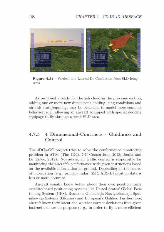
168 CHAPTER 4. CD IN 4D-AIRSPACE
Figure 4.34 – Vertical and Lateral De-Confliction from SLD-IcingArea
As proposed already for the ash cloud in the previous section,adding one or more new dimensions holding icing conditions andaircraft state/equipage may be beneficial to model more complexbehavior, e. g., allowing an aircraft equipped with special de-icingequipage to fly through a weak SLD area.
4.7.5 4 Dimensional-Contracts - Guidance andControl
The 4DCo-GC project tries to solve the conformance monitoringproblem in ATM (The 4DCo-GC Consortium, 2013; Joulia andLe Tallec, 2012). Nowadays, air traffic control is responsible formonitoring the aircraft’s conformance with given instructions basedon the available information on ground. Depending on the sourceof information (e. g., primary radar, SSR, ADS-B) position data isless or more accurate.
Aircraft usually know better about their own position usingsatellite-based positioning systems like United States’ Global Posi-tioning System (GPS), Russian’s Globalnaja Nawigazionnaja Sput-nikowaja Sistema (Glonass) and European’s Galileo. Furthermore,aircraft know their intent and whether current deviations from giveninstructions are on purpose (e. g., in order to fly a more efficient

4.7. APPLICATION IN PROJECTS 169
route) and therefore acceptable or if the guidance is physicallyunable to follow the instructions, e. g., given by a 4D-trajectory.
4DCo-GC puts the conformance monitoring responsibility intothe aircraft. In order to distinguish between allowed and severedeviations from a trajectory, a contract defining safety and freedommargins is negotiated between ground control and aircraft. Whileground control ensures that contracts of no two aircraft intersect,each aircraft has the task to stay in its assigned contract. For eachpoint in time, the contract defines allowed cross-track deviationsspecified in nautical miles, along-track deviations as a time, andvertical deviations as an allowed altitude offset. As soon as anaircraft forecasts that it cannot comply anymore with the givencontract, a new contract is calculated by the ground module.
Figure 4.35 shows how a contract is defined in the 4DCo-GCproject. The whole blue area around each aircraft is called contractbubble. An aircraft has a time-continuous contract bubble at eachtime from start to end of flight. For each time, the contract bubbleis safe from conflicts with all other contract bubbles. Contractbubble might touch each other, but not intersect. Contract bubblesare smaller around airports and bigger in less dense traffic situationlike en-route areas.
Aircraft are prevented to fly to the border of their contractsby the green safety bubble (SB). Safety bubbles must stay withinthe contract bubble in order to avoid dangerous contract violations.Thus, the allowed position of each aircraft is limited to the yellowfreedom bubble. The freedom bubble can be used by each aircraftto optimize efficiency of flight.
Assuming constant contract margins along time, conflict de-tection between contracts can be performed based on trajectoriesusing a separation adapted to the size of contract margins. Variablecontracts are much more difficult to handle, e. g., using morphingvolumes moving along a trajectory.
The NDMap was used within 4DCo-GC for generation of aconflict free scenario based on the optimized Europe sample. Sincethe optimized sample contains nearly 29 000 conflicts, effectiveconflict resolution algorithms were necessary in order to create a

170 CHAPTER 4. CD IN 4D-AIRSPACE
Contract Bubble
FreedomBubble FB
SB
ContractBubble
Freedom
BubbleFB
SB
Figure 4.35 – Contract Definition in the 4DCo-GC Project
conflict free sample. Conflict resolution algorithms are described inchapter 5.

Chapter 54D Conflict Resolution
As described in section 2.5, conflict resolution can either be per-formed laterally, vertically or time-based. The NDMap implemen-tation provides algorithms for all three types of conflict solution.All procedures use the trial-and-error method taking advantage ofthe high performance of the conflict detection algorithm.
Trial-and-error is not only facilitated by fast conflict detectiontimes (i. e., times for adding a new trajectory) but also by fast dele-tion times of 0.4 milliseconds for the German and 1.6 millisecondsfor the European sample. Thus, trajectories can be probed forconflicts in 2.0 ms (1.6 ms+0.4 ms) resulting in 500 trial-and-errorruns a second for the German sample and 1000 ms/(5.0+1.6) ms =151 probes a second for the European sample. Deletion times arethat high for the European sample because, for instance, conflictdeletion in the 29 k entries conflict vector is slow. Probing speedusually increases while reducing the number of remaining conflicts.
171

172 CHAPTER 5. 4D CONFLICT RESOLUTION
5.1 Global Trial-and-Error ConflictResolution
Conflict resolution is a complex task. Several issues need to betaken into account when trying to solve a conflict:
• The right of way is either given by a set of predefined rules(e. g., the EFR from section 2.5.6 on page 73) or dynamicallyassigned based on optimization metrics.
• The maneuver avoiding a conflict may create new conflictson the remaining route further downstream. Decision rulesneed to be defined if conflicts have different priorities (e. g.,depending on the flight phase), and whether moving a con-flict further downstream is an optimization and therefore apotential solution.
• Calculation of ambitious resolutions with minimum trajectorychange is usually more efficient, but also increases computa-tional effort.
• If multiple solutions are possible, the best solution needs to beidentified. Metrics are necessary to determine the preferredsolution.
Whether a conflict resolution is good or not needs to be welldefined. As for the global optimization of whole ATM, broadlyaccepted metrics are necessary to define the global optimum. ICAO(2005) defines following 11 expectations also known as Key Perfor-mance Areas (KPA) for the global ATM in alphabetical order:
• Access and equity.
• Capacity.
• Cost-effectiveness.
• Efficiency.
• Environment.

5.1. GLOBAL TRIAL-AND-ERROR CR 173
• Flexibility.
• Global interoperability.
• Participation by the ATM community.
• Predictability.
• Safety.
• Security.
Since the expectations are not independent conflicts of interestneed to be solved by a trade-off. An exception from the trade-offprocess is usually safety, since an acceptable safety is always highestpriority in aviation. Besides safety, keeping efficiency high is oneof the main factors when solving a conflict. However, also otherKPAs are relevant. Since the bottlenecks in ATM are usually theairports, holding an earlier accepted required time of arrival at thedestination airport is essential, ensuring the KPA predictability.
Regarding conflict resolution responsibility, there is also a trade-off between predictability and efficiency. Defining the right of wayaircraft according to a rule set like EFR increases predictability butmight not be the most efficient solution. The global optimum forthis decision might even be reached if both aircraft are responsibleto solve the conflict together, each solving a part of the conflict.
When performing trial-and-error conflict resolution, new probetrajectories need to be generated. Calculations can be performedwith different accuracy. While the complexity of trajectories is nota problem for the NDMap, it might be an issue for the (external)trajectory prediction engine not being able to deliver aircraft specificefficient trajectories fast enough.
It is not beneficial to use high accuracy trajectories for highfrequency conflict resolution testing for some reasons (Kuenz, 2011):
• Performance: The AFMS described in section 2.3.1 needs onaverage ∼ 100 ms to calculate realistic and flyable trajectoriesbased on aircraft model, list of waypoints, altitude, speed andtime constraints, and profile parameter. That is already pretty

174 CHAPTER 5. 4D CONFLICT RESOLUTION
fast compared to commercial FMS. However, the predictionof vertical and speed profiles is an iterative process. Thus,if altitude or time (e. g., required time of arrival) constraintsare tricky and difficult to meet, the prediction process mighttake up to 500 ms.
• Accuracy: Airborne trajectories are difficult to calculate by aground tool, considering a global ground based conflict resolu-tion tool. An aircraft knows best about its own performance.It provides up-to-date weather information by direct mea-surement in flight. Current aircraft weight is only known inaircraft, not on ground. Furthermore, airline specific proce-dures might not be published for ground tools. A study byStell (2010) on estimating descent trajectories of real flightswith a ground based tool illustrates difficulties localizing topof descent and predict meter fix times with high precision.
• Regeneration: When deviations occur in a flight, e. g., due tobad weather forecast, aircraft adapt their trajectories. Theseadaptations cannot be foreseen in the planning phase anyhow.
• Ambition: The best resolution maneuver is not the technicalsmart solution exactly fulfilling separation minima at any time.A more conservative approach with slightly worse efficiencyincluding some safety margins should be preferred to abateremaining uncertainties.
Therefore, the NDMap provides built-in conflict resolution algo-rithms generating simplified trial trajectories. Obstacle avoidancemaneuvers are generated
• Lateral, vertical and time-based.
• Based on performance indicators extracted from the initialtrajectory: Track-change, climb, descent, accelerate and de-celerate capabilities.
• If no resolution is found, deviation from original path issuccessively increased.
• If possible, avoidance maneuvers are generated for both con-flicting objects. The better solution gets implemented.

5.2. LATERAL RESOLUTION 175
• Providing simple metrics for solution rating. In the currentversion, route extension size and flight time are taken intoaccount.
Multiple conflicts are solved in chronological order. Result of theresolution process is a list of avoidance maneuvers, each containing:
• Reference to the object implementing the solution.
• Reference to the first conflict being solved.
• Number of conflicts being solved. Especially lateral andtime based solutions might solve (but also create) subsequentconflicts.
• Type of maneuver: climb x feet, descent x feet, avoid leftby x NM, avoid right by x NM, advance or delay flight by xseconds.
• Trial trajectory.
Anyhow, once having selected the best solution out of all trialtrajectories, a more precise AFMS trajectory should be generatedin order to validate the solution.
No matter how a conflict is solved, trial trajectories are alwaysgenerated for the complete remaining route. This way, downstreamconflicts can be taken into account. In the probing process, the trialtrajectory replaces the original conflicting trajectory. The updatedconflict list is compared to the original list of conflicts. If the newsituation is rated better, the probe trajectory is considered to be asolution. After probing with all foreseen trial trajectories is finished,the best rated solution, if any, is assigned as the solution of conflict.
5.2 Lateral Resolution
A lateral conflict resolution is shown in fig. 5.1. Calculation ofthe trial trajectories is mainly based on start and end of conflict.Trial trajectories are generated by moving the trajectory segmentbetween start and end of conflict orthogonal to its direction. In

176 CHAPTER 5. 4D CONFLICT RESOLUTION
Figure 5.1 – Lateral Resolution of Conflict
order to keep the rest of trajectory stable, two additional pointsare inserted before start of conflict and behind end of conflict. Thecorresponding δ is set to 120 seconds in the current version.
Although the figure shows for simplicity only probe trajectoriesdeviating to the right for one aircraft, probe trajectories are alwayscalculated for both aircraft in both directions, aiming for the overallbest solution. The parallel route offset starts with 0.5 NM and isincreased by 0.5 NM until finding a solution or reaching a predefinedmaximum.
Lateral conflict resolution has side-effects on the time. Theflight duration increases due to the lateral detour if speed staysunchanged. Both altitude and speed are assumed to be unchangedon the extra lateral segments. The resulting time variation producesa non-symmetric situation concerning left and right detour. Forthe conflict situation shown in fig. 5.1, the depicted solution isan efficient candidate. Compared to the time of original lateralintersection of trajectories, the aircraft from the south reaches thenew lateral intersection later due to the detour, and the aircraftfrom the east earlier. A deviation to the left delays the lateralintersection for both flights.
If and how this algorithm solves a conflict mainly depends onintersection angle, phase of flights, and speeds of aircraft. Lateral

5.3. VERTICAL RESOLUTION 177
Figure 5.2 – Vertical Resolution of Conflict
conflict resolution is not applicable for conflicts in the vicinityof airports. Obviously a lateral route offset is not possible on therunway, but usually also not reasonable in the dense airspace aroundairports.
5.3 Vertical Resolution
The vertical conflict resolution is depicted in fig. 5.2. Basically,the same algorithm as for the lateral resolution is applied. Thetrajectory segment between start and end of conflict is moved inaltitude. In order to leave the remaining trajectory unchanged,extra points are inserted before start and after end of conflict. Thecorresponding δ is set to 120 seconds per 1000 ft vertical deviation.
Again, probe trajectories are calculated for both aircraft in bothdirections. In contrast to the lateral resolution, the horizontal routelength stays the same. Assuming not too large altitude steps, climband descend speeds are of low importance, and times nearly stayunchanged. Altitude is increased and decreased by steps of 1000 ftas long as no solution was found or a maximum is reached.

178 CHAPTER 5. 4D CONFLICT RESOLUTION
Figure 5.3 – Time-Based Resolution of Conflict
At the runway threshold, also the vertical resolution is notapplicable due to the fixed threshold elevation. Depending on envi-ronmental constraints like noise sensitive areas, vertical resolutionscan be reasonable in the vicinity of airports. In the case the air-craft is in climb or descent, the procedure needs small adaptations.Climbing aircraft insert a level flight interrupting the climb in orderto dive below a conflict. Aircraft being close to their descent maybring forward part of it in order to create a lower conflict-resolvinglevel flight.
5.4 Time-Based Resolution
The main idea about time-based conflict resolution is reaching theconflict point’s original position at another conflict free time. Theoverflight time of a 3D-position (e. g., the start of conflict positionin fig. 5.3) can be adapted by different means.

5.4. TIME-BASED RESOLUTION 179
Assuming the aircraft is already airborne, overflight times canbe revised by speed variations and path shortening or stretching.As discussed before, path shortening requires doglegs in the initialroute to bypass, which are avoided in efficient route layouts. Onthe other hand, path stretching creates such doglegs and makesthe initial efficient routing inefficient. Thus, speed adjustment isthe proper mean to delay or advance an aircraft to avoid conflicts.However, assuming that original foreseen speeds are most efficientfor the given aircraft, adjustments also degrade overall performance.Furthermore, the δ in fig. 5.3 needs to be rather large, e. g., at atypical speed of 300 kts, δ needs to be ∼30 min to adjust overflighttime by 1 minute using a speed variation of 10 kts.
Assuming a strategic planning of air traffic where all aircraftare still on ground, a good way for time-based conflict avoidance isshifting the whole flight in time from departure to arrival.
5.4.1 Moving Whole Flights in Time
Shifting whole flights in time allows keeping flight duration constant.If a flight is shifted by few minutes only:
• Speed and altitude profiles can be assumed to stay unchangedcompared to the original route.
• Wind may change slightly due to different flight time, howeverthe influence is marginal and therefore negligible.
• Trajectories are as efficient as the initial trajectories.
• New trajectories can be calculated by decreasing/increasingtimes, no new profile needs to be calculated. Thus, predictionof trajectories is much faster.
Trying to adjust all trajectories of a scenario to get the optimumsolution is too complex even with very fast conflict detection andavoidance algorithms. Therefore, intelligent pre-selection of aircraftis necessary.
Figure 5.4 demonstrates the high traffic density. It containsFrankfurt/Main traffic with 1365 flights only (i. e. 4.1 %), extracted

180 CHAPTER 5. 4D CONFLICT RESOLUTION
from the European scenario. The coordinate system is time abovelatitude and longitude. The plot shows the whole day of traffic,with midnight on ground level and the end of day as upper delimiter.Trajectories are drawn in blue, with the conflicting segments inred. Figure 5.5 shows a close-up of the same data, scaling thetime-axis by factor 20 and moving the ground layer to t = 40 000 s.Since aircraft always climb when flying in XYT-notation, the flightdirection is directly visible, and type of conflicts can directly beextracted from the illustration.
Figure 5.4 – Flights from/to Frankfurt-Main as XYT-Diagram 24h
5.4.1.1 Global Algorithm
The global algorithm moves trajectories in time in order to reducescenario’s conflict count. First of all, conflicts of the scenario aresorted chronologically. Cycling through all conflicting objects, timeshifts are implemented on the corresponding trajectories using stepsof 10 seconds up to a maximum shift time, e. g., 10 minutes. Af-terwards, the trajectories are probed against the complete scenario.As soon as a conflict is solved by the shifting operation and thetotal number of conflicts for the corresponding flight is also reduced,the solution is considered to be the new trajectory for this flight.

5.4. TIME-BASED RESOLUTION 181
Figure 5.5 – Flights from/to Frankfurt-Main as XYT-Diagramaround Noon
5.4.1.2 Recursive Algorithm
Also the recursive algorithm tries to solve conflicts chronologically.Conflicting aircraft are moved in time in steps of 5 s in order to re-solve the conflict. Having already applied the global algorithm, thiswill typically not produce a proper solution because it is basicallythe same procedure as above described global conflict solution algo-rithm except from the finer granularity of 5 s. The main differenceis the handling of generated conflicts. Since the conflict detectionalgorithm validates the whole trajectory for conflicts, follow-upconflicts are well known for each probe trajectory.
Probe trajectories generating more follow-up conflicts than hav-ing solved before are skipped by the global algorithm. In contrast,the recursive algorithm validates if generated follow-up conflicts canbe avoided by time shift. As soon as conflict with a new aircraftarises this aircraft is also shifted by 5 s in the appropriate direction.Thus, that new conflict is immediately solved by re-establishing theoriginal distance. Since this might produce another conflict withanother aircraft, this algorithm is performed recursively and mightmove several aircraft simultaneously. The recursion is stopped at a

182 CHAPTER 5. 4D CONFLICT RESOLUTION
Arrival 1
Arrival 2
Arrival 3 Arrival 4 Arrival 5Arrival 0
Arrival 1 Arrival 2 Arrival 3 Arrival 4 Arrival 5Arrival 0
Arrival Slots
Figure 5.6 – Solving Conflicts Recursively
predefined depth (e. g., 10). Since moving an aircraft by 5 s mightproduce several conflicts all along the whole trajectory, recursiveconflict resolution may become computational complex for highdensity scenario. As soon as a conflict cannot be resolved with thegiven recursion depth, disadvantageous operations are undone.
Figure 5.6 shows the general idea using the example of an arrivalladder. Above the arrival slot ladder, the conflict is displayed. Ar-rival 2 is in conflict with arrival 1. However, due to bad distributionof arrival 3 and arrival 4, there is no free slot for arrival 2. Thedescribed algorithm delays arrival 2 until detecting a new conflictwith arrival 3. Since arrival 3 is the first aircraft producing a newconflict, it is also delayed. This produces another conflict betweenarrival 3 and arrival 4. By delaying all three arrivals furthermore, asolution can be found that is depicted below the arrival slot ladder.The solution implies that delaying the mentioned flights does notgenerate new conflicts somewhere else.
If delaying arrival 3 had generated a new conflict at its departureor in its en-route segment, the corresponding successor also wouldhave been delayed.
Summarizing, this algorithm does not only focus on aircraft inconflict situations but also shifts aircraft non-involved in conflictsin order to make room for conflict solutions.
Furthermore, this algorithm implements a shared conflict reso-lution when possible. If no solution can be found for arrival 2in fig. 5.6, the flight is nevertheless delayed as much as possiblewithout creating new conflicts. Thus, arrival 2 can already solve

5.5. DECONFLICTING OPTIMIZED TRAFFIC 183
one part of the conflict. The remaining part of the conflict can bepotentially solved by bringing forward arrival 1.
5.4.2 Flight Duration Adaptation
Another mean of solving conflicts time-based is changing the du-ration of flight. Due to the assumption that the initial flight’sefficiency is optimized, this degrades the performance. However,if traffic density is too high, constant flight duration constrainsthe number of solvable conflicts. In order to be still as efficient aspossible, small adaptations should be preferred.
Flight duration adaptations should also take into account:
• Overall flight duration: long haul flights can handle higheradaptations than short haul flight.
• Aircraft model: some aircraft have a tight flight enveloperegarding speed. Others allow changing speed in a biggerinterval.
• Aircraft’s efficiency: concerning global efficiency, it is moreefficient to penalize efficient aircraft, and allow less efficientaircraft to fly their optimum route. However, this wouldprivilege inefficient aircraft which does not sound like a fairidea. A well balanced trade-off between the KPAs needs toincorporate access and equity to ensure overall fairness.
5.5 Deconflicting European’s Opti-mized Traffic
This section describes deconfliction trials based on the Europeantraffic sample described in section 4.2.2 on page 139. Figure 5.7shows the conflicts of the optimized scenario where each aircraftflies its preferred route. Conflicts are illustrated by red trajectorysegments. Thus, short conflicts (e. g., rectangular intersections) arerather small, while two aircraft sharing the same route with a toosmall time offset are quite long.
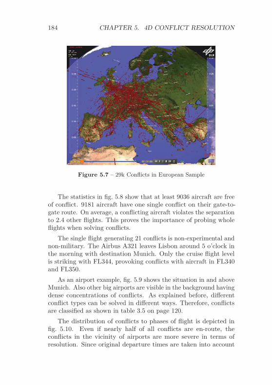
184 CHAPTER 5. 4D CONFLICT RESOLUTION
Figure 5.7 – 29k Conflicts in European Sample
The statistics in fig. 5.8 show that at least 9036 aircraft are freeof conflict. 9181 aircraft have one single conflict on their gate-to-gate route. On average, a conflicting aircraft violates the separationto 2.4 other flights. This proves the importance of probing wholeflights when solving conflicts.
The single flight generating 21 conflicts is non-experimental andnon-military. The Airbus A321 leaves Lisbon around 5 o’clock inthe morning with destination Munich. Only the cruise flight levelis striking with FL344, provoking conflicts with aircraft in FL340and FL350.
As an airport example, fig. 5.9 shows the situation in and aboveMunich. Also other big airports are visible in the background havingdense concentrations of conflicts. As explained before, differentconflict types can be solved in different ways. Therefore, conflictsare classified as shown in table 3.5 on page 120.
The distribution of conflicts to phases of flight is depicted infig. 5.10. Even if nearly half of all conflicts are en-route, theconflicts in the vicinity of airports are more severe in terms ofresolution. Since original departure times are taken into account
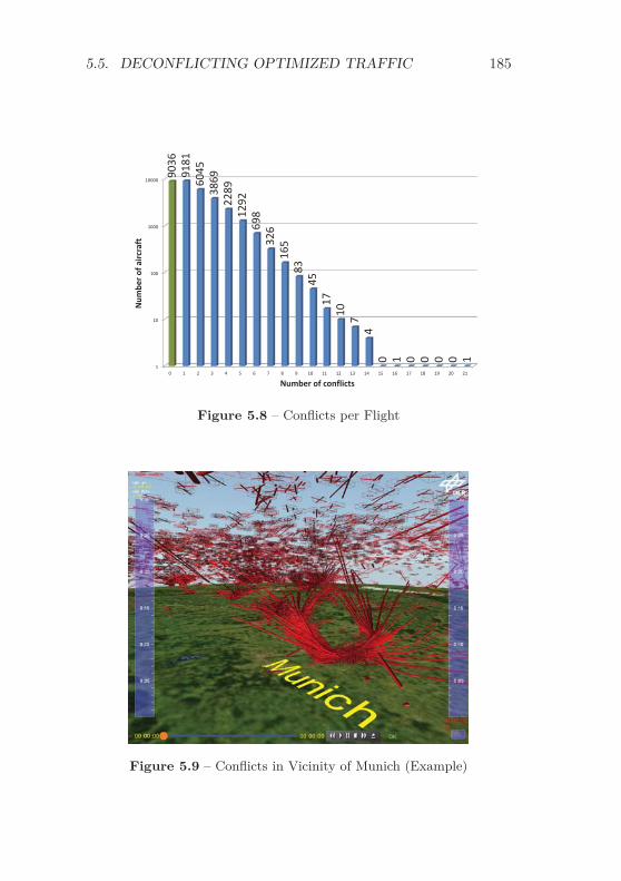
5.5. DECONFLICTING OPTIMIZED TRAFFIC 185
1
10
100
1000
10000
0 1 2 3 4 5 6 7 8 9 10 11 12 13 14 15 16 17 18 19 20 21
9036
91
81
6045
38
69
2289
12
92
698
326
165
83
45
17
10
7 4
0 1 0 0 0 0 1
Num
ber o
f airc
raft
Number of conflicts
Figure 5.8 – Conflicts per Flight
Figure 5.9 – Conflicts in Vicinity of Munich (Example)

186 CHAPTER 5. 4D CONFLICT RESOLUTION
7994
1150
6467
13375
ArrivalDeparture Arr/DepOther
Figure 5.10 – Conflicts by Flight Phase
when optimizing the scenario, flights are separated at the departurerunway threshold and thus the number of departure conflicts is low.Having departure conflicts at all can be reasoned by:
• Misinterpreted departure runways from the original data.Especially departures (and also arrivals) from parallel runwaysare difficult to distinguish.
• Inaccurate data with insufficient resolution.
• Too conservative conflict metrics. ICAO (2007) defines specialprocedures for, e. g., parallel or near-parallel runways (chapter6.7: Operations on Parallel or Near-Parallel Runways) allow-ing a separation below 3 NM. This accounts for departureand arrival traffic.
Arrival and departure/arrival conflicts are as expected becausearrival times changed with more direct routes and optimized speedprofiles.
Depending on a conflict’s classification different solution methodscan be applied. As described before, there are obvious restrictionsfor conflict resolution close to runway threshold:
• Since the threshold height is fixed, it is not possible to providea vertical solution.
• Lateral solution is feasible only for airports with multiplerunways and when the arrival runway is not fixed.

5.5. DECONFLICTING OPTIMIZED TRAFFIC 187
• Time-based solution is the most promising way to solve con-flicts on the thresholds.
The limited possibilities for conflict resolution at the runway thre-sholds advises to solve threshold conflicts first using time-basedshifting of trajectories as described in section 5.4.1.1.
5.5.1 Airport-Focused Conflict Resolution
A significant reduction of conflicts already can be reached with amaximum time shift of [-30 s, +30 s]. The number of airport locatedconflicts reduces to ∼64 %. Figure 5.11 depicts the remainingconflicts for each category. Even though the algorithm focuses onconflicts in airport vicinity, also en-route conflicts are reduced as aspin-off from trajectory movement.
5670 525
3757
11881
ArrivalDeparture Arr/DepOther
Figure 5.11 – Conflicts afterShift of ±30 seconds
791 97 484
7253
ArrivalDeparture Arr/DepOther
Figure 5.12 – Conflictsafter Shift of ±10 minu-tes
Allowing a time shift of [-10 min, +10 min], airport conflicts arereduced to ∼9 % (fig. 5.12), still without touching the scenario’sefficiency. Figure 5.13 illustrates how the number of airport relatedconflicts can be reduced with the corresponding maximum allowedtime offset. The top of the blue bars represents the number ofremaining airport-related conflicts.
Applying the recursive time shift described in section 5.4.1.2,conflicts at the airport can be further reduced to ∼6 % of initialairport conflicts (fig. 5.14) with a maximum recursion depth of 10.

188 CHAPTER 5. 4D CONFLICT RESOLUTION
0
5000
10000
15000
20000
25000
30000
0 30 60 90 120 150 180 210 240 270 300 330 360 390 420 450 480 510 540 570 600
Num
ber o
f Con
flict
s
Maximum Time-Offset in Seconds
Other Arr/Dep Departure Arrival
Figure 5.13 – Airport-Focused Reduction in Relation to Time-Shift
452 81 410
6305
ArrivalDeparture Arr/DepOther
Figure 5.14 – Recursive Op-timization Level 10
404 59 366
6132
ArrivalDeparture Arr/DepOther
Figure 5.15 – Recursive Op-timization Level 20
Figure 5.15 shows the results for an extended recursion depth of 20leaving 829 remaining conflicts close to airports.
5.5.2 Global Conflict Resolution
For a global conflict resolution, all conflicting trajectories are probedby movement in time without focusing on airport conflicts. Startingscenario is the outcome from the airport-related conflict resolution

5.5. DECONFLICTING OPTIMIZED TRAFFIC 189
described before. In order to avoid creation of new airport relatedconflicts as a possible side-effect from multiple en-route resolutionsa weighting of conflicts is introduced. Therefore, airport-relatedconflicts are defined to be 10 times more severe than en-routeconflicts. This ensures that no trade-off is done between en-routeand airport conflicts in favor of en-route conflicts. In contrast,the weighting factor even supports solving further airport-relatedconflicts with the trade-off of generating new en-route conflicts.
0
1000
2000
3000
4000
5000
6000
7000
0 30 60 90 120 150 180 210 240 270 300 330 360 390 420 450 480 510 540 570 600
Num
ber o
f Con
flict
s
Maximum Time-Offset in Seconds
Other Arr/Dep Departure Arrival
Figure 5.16 – Global Reduction in Relation to Time-Shift
The progress of the global time shifting is shown in fig. 5.16. Thetotal number of conflicts can be reduced drastically. The weightingof conflicts does not only preserve resolutions for airport relatedconflicts but even allows further reduction. The distribution ofconflicts with a time shift of ±10 minutes is depicted in fig. 5.17.After applying the recursive algorithm with a maximum recursiondepth of 20, the final distribution shown in fig. 5.18 is achieved.Thus, initially ∼29 k conflicts can be reduced to 1647 withoutdecreasing aircraft’s efficiency.

190 CHAPTER 5. 4D CONFLICT RESOLUTION
347 26
181 1470 ArrivalDeparture Arr/DepOther
Figure 5.17 – Conflicts afterGlobal Shift of ±10 minutes
316 23
156 1152
ArrivalDeparture Arr/DepOther
Figure 5.18 – Global Recur-sion Optimization Level 20
5.5.3 Resolution of En-Route Conflicts
En-route conflicts can be reduced further with lateral and verticalmaneuvers. Due to the weighting of airport versus en-route conflictsthis even further reduces the number arrival conflicts. The resultafter lateral and vertical resolution leaving less than 500 conflicts isshown in fig. 5.19.
319 23 144 10
ArrivalDeparture Arr/DepOther
Figure 5.19 – Conflicts afterLateral and Vertical Resolu-tion
Figure 5.20 – Very ShortEn-route Conflict in Red
Obviously, not all conflicts are solvable with the algorithmsapplied. Figure 5.20 shows one example for a remaining en-routeconflict. Flight DLRLC departed from Paris-Charles-de-Gaulle, isstill in climb and heads for the United States. Flight DLR9MWdeparted from London-Stansted, already reached cruise FL370, andheads for Murcia-San Javier. Both flights have a conflict accordingto the selected conflict metrics for as short as 0.7 seconds. Theclosest point of approach is reached when DLR9MW passed thepath intersection

5.5. DECONFLICTING OPTIMIZED TRAFFIC 191
Figure 5.21 – Remaining Conflicts
All remaining conflicts are depicted in fig. 5.21. Conflicts areconcentrating on major European airports like Paris-Charles-de-Gaulle, Amsterdam Schiphol, London-Heathrow, Rome-Fiumicino,Frankfurt Main, Zurich, and Munich Franz Josef Strauss. Mostof the mentioned airports have a parallel or near-parallel runwaysystem allowing reduced separation for parallel approaches anddepartures. Thus, at least some of the remaining conflicts are noconflicts in real life thanks to special operations allowing closerseparation.
Since this work focuses on conflict detection and resolutionwhile the exact specification of a conflict is done by the user by theexternal conflict function, this adaptation is not handled here.
Furthermore, not all effort was put yet into solving conflicts.One parameter not adapted yet is the flight duration. Thus, tryingto solve an arrival conflict by delaying an arrival by 10 seconds

192 CHAPTER 5. 4D CONFLICT RESOLUTION
relies on the freedom to simultaneously delay the departure by also10 seconds so far. Allowing to change the flight duration offersa good potential to solve the remaining conflicts. However, theaforementioned improvement on conflict specification should bedone first in order to guarantee that a conflict-free solution existsin terms of airport load.
In order to get a conflict free scenario for the 4DCo-GC project,another conflict resolution method was applied. The remaining 496conflicts were solved by flight cancellation. Although deletion ofone aircraft from each conflict reduces the total number of aircraftto 32 573, it ensures a still big and conflict-free scenario.

Chapter 6Verification and Validation
This chapter describes a verification and validation of the softwaremodule developed in this work. According to Boehm (1979), vali-dation and verification formulate different questions concerning thequality of a software project:
• Validation: "Are we building the right product?"
• Verification: "Are we building the product right?"
Since the product generated in this work was not created accordingto explicitly defined product requirements it is nevertheless difficultto distinguish between verification and validation. The developmentof the NDMap started with the rough idea of subdividing airspace inall 4 dimensions in order to allow efficient conflict detection. Whilethe basic concept remained, promising results with big scenarios ledto an extensive usage in projects all formulating their own require-ments. Verification (or according to Popper (1974) falsification) ofthe software is usually done on programming via testing softwareinvariants.
In order to validate that the software is reasonable for its opera-tional purpose, several use cases are checked below. Each use casecontains the scenario description in a Keyhole Markup Language
193

194 CHAPTER 6. VERIFICATION AND VALIDATION
(KML) like style1, a screenshot showing the result, and a printoutfrom the corresponding NDMap object. All scenarios are completelyfictional and do not represent reality. The trajectories are artificialand do not necessarily take aircraft performance parameter intoaccount. Conflict detection is done with the aforementioned metricsof 5 NM lateral and 1000 ft vertical.
6.1 Nominal Case
The scenario described in listing 6.1 defines one trajectory from Westto East at 50° latitude and three additional trajectories crossingthe first in different angles. Figure 6.1 depicts the resulting threeconflicts. As expected, the rectangular intersection results in ashort conflict, while the most pointed intersection has a muchbigger extension.
Listing 6.2 shows the corresponding NDMap output.Thus, the NDMap object uses 119.5 KiB of memory with a total
number of 415 generated tiles. Average time to add a trajectory was0.48 ms. Three conflicts were detected with duration from 13.9 s to57.5 s.
6.2 Pseudo-Parallel Case
The scenario described in listing 6.3 defines two trajectories goingexactly from South to North with a constant longitudinal distanceof 0.1°. Both trajectories start at the Equator where a tenth of adegree approximates conflict-free 6 NM. Going further to the North,the corresponding distance to a tenth of degree decreases, andtherefore results in a conflict beginning at the latitude where cos ϕ =5/6. Thus, the conflict should start at arccos(5/6) = 33.56° =33°33.6′ on a sphere. However, the implementation uses Vincenty’sformula based on WGS84 ellipsoid where the Equatorial radiusis slightly bigger compared to common sphere models (compare
1Note that altitudes are defined in meters in KML but converted to feet inthe NDMap, latitudes and longitudes are converted from degree to radian

6.2. PSEUDO-PARALLEL CASE 195
Listing 6.1 – Nominal Case Scenario
<Placemark id="EASTWEST"> <name>EASTWEST</name> <coordinates>
60,50,10000,100000,50,10000,16000</coordinates> </Placemark>
<Placemark id="SOUTHNORTH"> <name>SOUTHNORTH</name> <coordinates>
10,0,10000,1000010,60,10000,16000</coordinates> </Placemark>
<Placemark id="DEG45"> <name>DEG45</name> <coordinates>61,0,10000,99001,60,10000,15900</coordinates> </Placemark>
<Placemark id="DEG10"> <name>DEG10</name> <coordinates>28,45,10000,12100-10,55,10000,18100</coordinates> </Placemark>
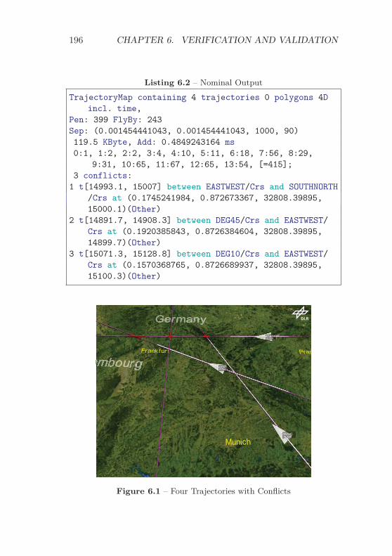
196 CHAPTER 6. VERIFICATION AND VALIDATION
Listing 6.2 – Nominal Output
TrajectoryMap containing 4 trajectories 0 polygons 4Dincl. time,
Pen: 399 FlyBy: 243Sep: (0.001454441043, 0.001454441043, 1000, 90)119.5 KByte, Add: 0.4849243164 ms0:1, 1:2, 2:2, 3:4, 4:10, 5:11, 6:18, 7:56, 8:29,
9:31, 10:65, 11:67, 12:65, 13:54, [=415];3 conflicts:
1 t[14993.1, 15007] between EASTWEST/Crs and SOUTHNORTH/Crs at (0.1745241984, 0.872673367, 32808.39895,15000.1)(Other)
2 t[14891.7, 14908.3] between DEG45/Crs and EASTWEST/Crs at (0.1920385843, 0.8726384604, 32808.39895,14899.7)(Other)
3 t[15071.3, 15128.8] between DEG10/Crs and EASTWEST/Crs at (0.1570368765, 0.8726689937, 32808.39895,15100.3)(Other)
Figure 6.1 – Four Trajectories with Conflicts

6.2. PSEUDO-PARALLEL CASE 197
Listing 6.3 – Pseudo-Parallel Scenario
<Placemark id="EAST"> <name>EAST</name> <coordinates>10,0,10000,1000010,60,10000,16000</coordinates> </Placemark>
<Placemark id="WEST"> <name>WEST</name> <coordinates>9.9,0,10000,100009.9,60,10000,16000</coordinates> </Placemark>
Listing 6.4 – Pseudo-Parallel Output
TrajectoryMap containing 2 trajectories 0 polygons 4Dincl. time,
Pen: 5014 FlyBy: 1661Sep: (0.001454441043, 0.001454441043, 1000, 90)1.1 MByte, Add: 7.225585938 ms0:1, 1:2, 2:1, 3:3, 4:5, 5:9, 6:18, 7:66, 8:64, 9:134,
10:542, 11:459, 12:854, 13:1574, [=3732];1 conflicts:
1 t[13380.1, 16000] between EAST/Arr and WEST/Arr at(0.173660256, 1.047040501, 32808.39895, 15999.1)(Arrival)
section 2.6.1). Therefore, based on the more precise WGS84 model,the conflict starts at ∼33°50′ and remains active until reaching endof trajectories.
Figure 6.2 depicts the resulting conflict. Listing 6.4 holds theresults from the corresponding NDMap.
As discussed earlier, nearly identical trajectories cause creationof many nodes, 3732 in total. Also the memory usage of 1.1 MiBand detection times of 7.2 ms are above typical average.

198 CHAPTER 6. VERIFICATION AND VALIDATION
Figure 6.2 – Pseudo-Parallel Trajectories
6.3 Conflict Jitter Case
This use-case is supposed to validate the anti-jitter functionalitydescribed in section 3.5.3. Therefore, the scenario described inlisting 6.5 defines two trajectories flying mostly parallel from Westto East, one with a constant latitude of 50° while the other onevaries between 49.9° and 49.95°. A tenth of degree latitude approx-imates conflict-free 6 NM, while a twentieth degree approximates toconflicting 3 NM. As defined by the input file, conflict distance isunderrun three times. However, the first two conflicts are mergedinto one because the distance in-between is too short. The thirdconflict is too far away to get merged.
Figure 6.3 depicts the resulting conflicts. Listing 6.6 shows theresults from the corresponding NDMap.
As experienced with the pseudo parallel case, conflict detectionis rather slow and memory consuming due to nearly identical routes.The first conflict starting at t =10 133 s is the union of the first twoseparation violations.

6.3. CONFLICT JITTER CASE 199
Listing 6.5 – Jitter Scenario
<Placemark id="NORTH"> <name>NORTH</name> <coordinates>0,50,10000,1000060,50,10000,16000</coordinates> </Placemark>
<Placemark id="SOUTH"> <name>SOUTH</name> <coordinates>0,49.9,10000,100001,49.9,10000,101002,49.95,10000,102003,49.95,10000,103004,49.9,10000,104005,49.95,10000,105006,49.95,10000,106007,49.9,10000,1070011,49.9,10000,1110012,49.95,10000,1120013,49.95,10000,1130014,49.9,10000,1140060,49.9,10000,16000</coordinates> </Placemark>

200 CHAPTER 6. VERIFICATION AND VALIDATION
Listing 6.6 – Jitter Output
TrajectoryMap containing 2 trajectories 0 polygons 4Dincl. time,
Pen: 654 FlyBy: 434Sep: (0.001454441043, 0.001454441043, 1000, 90)184.0 KByte, Add: 1.068359375 ms0:1, 1:2, 2:1, 3:2, 4:3, 5:6, 6:13, 7:44, 8:84, 9:22,
10:41, 11:66, 12:228, 13:126, [=639];2 conflicts:
1 t[10133.6, 10666.5] between NORTH/Crs and SOUTH/Crsat (0.05229006584, 0.8722282946, 32808.39895,10299.6)(Other)
2 t[11133.5, 11366.4] between NORTH/Crs and SOUTH/Crsat (0.2095267825, 0.8722282946, 32808.39895,11200.5)(Other)
Figure 6.3 – Jitter in Conflict

6.4. SINGULARITY CASE 201
Listing 6.7 – Pole Scenario
<Placemark id="POLE1"> <name>POLE1</name> <coordinates>-90,50,10000,10000-90,90,10000,16000</coordinates> </Placemark>
<Placemark id="POLE2"> <name>POLE2</name> <coordinates>90,50,10000,1000090,90,10000,16000</coordinates> </Placemark>
Listing 6.8 – Pole Output
TrajectoryMap containing 2 trajectories 0 polygons 4Dincl. time,
Pen: 1380 FlyBy: 3317Sep: (0.001454441043, 0.001454441043, 1000, 90)803.2 KByte, Add: 4.845458984 ms0:1, 1:3, 2:4, 3:6, 4:8, 5:12, 6:52, 7:100, 8:99,
9:204, 10:413, 11:609, 12:1006, 13:272, [=2789];1 conflicts:
1 t[15993.8, 16000] between POLE1/Arr and POLE2/Arr at(0, 1.570773099, 32808.39895, 15999.8)(Arrival)
6.4 Singularity Case
The scenario described in listing 6.7 defines two trajectories flyingexactly from South to North, starting at a latitude of 50° and endingat the North Pole 90°. The trajectories are located on oppositesides of Earth at longitudes of −90° and 90°. Both trajectoriesreach North Pole in same altitudes at the same time.
Figure 6.4 depicts the resulting conflict above North Pole. Thecorresponding NDMap output is shown in listing 6.8.

202 CHAPTER 6. VERIFICATION AND VALIDATION
Figure 6.4 – Conflict at North Pole
As already explained in section 4.1.1 the optimal representationcontains only one longitudinal tile at the Poles. Due to the treestructure each tile contains its children, and multiple tiles aregenerated close to the Poles. Thus, the NDMap generates a ratherhigh total number of 2789 nodes. However, the conflict at the NorthPole is detected reliably.
6.5 Discontinuity Case
The scenario described in listing 6.9 defines three trajectories. Twoaircraft fly exactly from South to North at longitudes 179.98° Eastand West respectively. The third trajectory intersects the datelineat the Equator.
Figure 6.5 depicts the two resulting conflicts. The pseudo parallelroutes are in conflict constantly. The East-West trajectory is inconflict with the flight at longitude 179.98° East. The NDMapoutput is shown in listing 6.10.

6.5. DISCONTINUITY CASE 203
Listing 6.9 – Discontinuity Scenario
<Placemark id="WEST"> <name>WEST</name> <coordinates>-179.995,-50,10000,10000-179.995,50,10000,15950</coordinates> </Placemark>
<Placemark id="EAST"> <name>EAST</name> <coordinates>179.995,-50,10000,10000179.995,50,10000,15950</coordinates> </Placemark>
<Placemark id="EASTWEST"> <name>EASTWEST</name> <coordinates>
178,1,10000,12500-178,-1,10000,13500</coordinates> </Placemark>
Listing 6.10 – Discontinuity Output
TrajectoryMap containing 3 trajectories 0 polygons 4Dincl. time,
Pen: 4041 FlyBy: 8300Sep: (0.001454441043, 0.001454441043, 1000, 90)2.3 MByte, Add: 5.306966146 ms0:1, 1:4, 2:6, 3:13, 4:17, 5:29, 6:55, 7:102, 8:102,
9:392, 10:788, 11:1410, 12:2679, 13:2546, [=8144];2 conflicts:
1 t[10000, 15950] between EAST/Dep and WEST/Dep at (0,-0.8726646304, 32808.39895, 10000)(Departure)
2 t[12975.9, 12980.9] between EAST/Crs and EASTWEST/Crsat (3.140681647, 0.0009402631346, 32808.39895,
12978.9)(Other)

204 CHAPTER 6. VERIFICATION AND VALIDATION
Listing 6.11 – Internal Representation of EASTWEST Trajectory
Trajectory for EASTWEST(6 Points)(3.106686115, 0.01745329238, 32808.39895, 12500)(3.14158637, 3.141596834e-06, 32808.39895, 12999.91)(3.14158637, 3.141596834e-06, 1e+30, 12999.911)(-3.14158637, -3.141596834e-06, 1e+30, 13000.089)(-3.14158637, -3.141596834e-06, 32808.39895, 13000.09)(-3.106686115, -0.01745329238, 32808.39895, 13500)
Figure 6.5 – Conflicts at Date Line
As experienced earlier, the NDMap generates a rather highamount of nodes due to parallelism of EAST and WEST. Listing 6.11shows a dump of the internal EASTWEST trajectory. The firstand last points are the original points of the trajectory, while points2-5 are automatically generated. Point 2 and point 5 hold theinterpolated positions just before and after passing the date-line.Point 3 and point 4 hold the connection between point 2 and point 5not lying in the NDMap’s interval at an altitude of 1030 ft.

6.6. POLYGON VOLUME CASE 205
6.6 Polygon Volume Case
The scenario described in listing 6.12 defines three objects. Twoflights are defined by trajectories. DLR1 departs from Nurembergwith direction South-East. DLR2 crosses the Southern part ofGermany from West to East.
The third object called Germany is a polygon volume approxi-mating the German borders. The scenario importer uses minimumand maximum altitudes for a volume object as lower and upperboundaries. Thus, the German polygon has a lower boundary of8000 meters and goes up to 11 300 meters.
Figure 6.6 depicts the three resulting conflicts. The trajectoriesare not in conflict with each other. DLR1 has a conflict between8000 and 11 300 meters with the polygon volume. DLR2 has twoconflicts with the German polygon interrupted by the non-Germanpart of Lake Constance. The NDMap output is shown in listing 6.13.
The NDMap generates a rather low amount of nodes (35), uses10.1 KiB of memory only. The average detection time per objectis 0.11 ms. This good performance is reached by means of the fullcontainment technique described in section 3.3.5.
Adding the lines from listing 6.14 to the German polygon volumemakes the volume move in time. The polygon volume appears attime zero (i. e., midnight). At time 36 000 s (i. e., ten o’clock) thepolygon is supposed to be 5000 meters lower. At noon (43 200 s),the polygon is still 5000 meters below start condition. Thereafter,the polygon is no more valid and disappears. Between the giventimes, the polygon state is linearly interpolated. Thus, the wholepolygon descends continuously between midnight and ten o’clockand stays there until noon.
This modification has two effects that are visible in the NDMapoutput (listing 6.15). The volume is already below DLR2 when itenters the polygon’s boundaries laterally. Therefore, there are nomore conflicts with DLR2. The conflict with DLR1 starts earlierbecause of the reduced altitude and has a shorter duration becausethe aircraft climbs while the volume descends.

206 CHAPTER 6. VERIFICATION AND VALIDATION
Listing 6.12 – Polygon Volume Scenario
<Placemark id="DLR1"><name>DLR1</name><coordinates>11.103056,49.493333,548.6,303.012.603611,49.085278,9022.1,973.013.360278,48.750833,11338.6,1257.013.490833,48.659444,11704.3,1318.013.606667,48.561944,11856.7,1379.015.108611,47.255000,11887.2,2195.0</coordinates>
</Placemark><Placemark id="DLR2">
<name>DLR2</name><coordinates>5.544444,48.245278,11277.6,3957.015.106944,46.899167,11277.6,6733.0</coordinates>
</Placemark><Placemark id="GERMANY">
<name>GERMANY</name><LinearRing><coordinates>
6.499999, 54.999989,113007.999998, 54.999989,80008.333332, 55.066655...[many points skipped to increase readability]...6.499999, 53.6666566.499999, 54.999989
</coordinates></LinearRing>
</Placemark>

6.6. POLYGON VOLUME CASE 207
Listing 6.13 – Polygon Volume Output
TrajectoryMap containing 2 trajectories 1 polygon 4Dincl. time,
Pen: 52 FlyBy: 0Sep: (0.001454441043, 0.001454441043, 1000, 90)10.1 KByte, Add: 0.1146647135 ms0:1, 1:3, 2:4, 3:5, 4:6, 5:16, [=35];3 conflicts:
1 t[892.1825376, 1252.267736] between DLR1/Clb andGERMANY/Poly at (0.2168154297, 0.8575587731,26246.71916, 892.1825376)(Polygon)
2 t[4673.562491, 4806.546029] between DLR2/Crs andGERMANY/Poly at (0.1398495709, 0.8359744606,36999.99872, 4673.562491)(Polygon)
3 t[5140.595825, 5807.581754] between DLR2/Crs andGERMANY/Poly at (0.1679282864, 0.8320218268,36999.99872, 5140.595825)(Polygon)
Figure 6.6 – Conflicts with Germany Volume

208 CHAPTER 6. VERIFICATION AND VALIDATION
Listing 6.14 – Trajectory for German Polygon Volume
<LineString><coordinates>
0,0,0,00,0,-5000,360000,0,-5000,43200
</coordinates></LineString>
Listing 6.15 – Moving Polygon Volume Output
TrajectoryMap containing 2 trajectories 1 polygon 4Dincl. time,
Pen: 46 FlyBy: 0Sep: (0.001454441043, 0.001454441043, 1000, 90)8.6 KByte, Add: 2.865722656 ms0:1, 1:2, 2:2, 3:3, 4:6, 5:16, [=30];1 conflicts:
1 t[882.6, 1231.3] between DLR1/Dep and GERMANY/Poly at(0.2164564936, 0.857656381, 25865.7097, 883)(
Polygon)

Chapter 7Conclusions and Outlook
This document describes a new and high performance method forconflict detection between multi-dimensional objects. Allowingto model problems with an arbitrary number of dimensions, theproposed algorithm offers a wide range of applications. The basicidea of the algorithm is an N -dimensional bisection of (air)spaceuntil reaching a given separation size. In order to achieve a goodperformance regarding calculation times and memory usage, severaltechniques were applied:
• Special handling of a selectable common time/reference dimen-sion reduces overall memory usage and increases performance.
• Instead of considering neighborhood of tiles, the algorithmdistinguishes between fly-through and fly-by objects alreadywhen building the tree.
• The algorithm is optimized to detect symmetric situationsonce only. This especially applies for fly-by situations whereone fly-by object is already omitted when building the tree.
• Large polygons are optimized by the full containment checkin order to avoid unnecessary subdivisions.
209

210 CHAPTER 7. CONCLUSIONS AND OUTLOOK
• Conflict detection is sped up by checking bounding boxes first.
• Monotony of dimensions is used beneficially, for example, byapplying binary search.
• Trials with different input value balancing techniques did notimprove performance.
• If the user has a focus on a subset of objects, preselection func-tionality of objects is provided increasing conflict detectionspeed significantly.
• Running the algorithm on a system with low memory is facili-tated by both static and dynamic memory saving mechanisms.
Conflict detection can be performed for N -dimensional trajecto-ries and N -dimensional polygon volumes. Furthermore, a trajectorycan be assigned to a polygon volume in order to model a volumemovement. The result of the tiling algorithm is a list containing alldetected conflicts.
Furthermore, a mapping is described from Earth-coordinatesto the Cartesian coordinate system used in the tiling algorithm. Aspecial Earth mode implemented in the NDMap respects furtheradaptations like non-uniform size of longitudes and avoidance ofsingularity issues at Poles and date line.
Based on a German and European traffic scenario, performancetests yield 1.6 ms detection time using 68 KiB per trajectory and5 ms detection time using 120 KiB per trajectory respectively.
Based on these promising results, conflict resolution was per-formed in a trial-and-error manner with 151 probes a second onthe European traffic sample. Since conflicts at the airports offerlimited possibilities for resolution (i. e., usually only time-based), afocus was put onto solving airport related conflicts first.
Conflict solving was performed on an optimized European traf-fic sample flying most direct routes with aircraft-optimized flightprofiles containing ∼29 000 conflicts initially. Allowing a maximumtime shift of ±10 minutes, conflicts were reduced to 1647 withoutdegrading aircraft’s efficiency. Applying lateral and vertical reso-

211
lution algorithms on the remaining conflicts, overall conflict countcan be reduced to 496.
Further freedom to solve conflicts lies in the adaptation offlight times that are still untouched. However, a better modelingof separation minima for arrival and departure traffic should beintegrated first in order to respect, for example, relaxed separationrequirements in independent parallel runway operations.
One main goal at implementation level was to keep the solutionas generic as possible. This also applies for further enhancements.Thus, parallel runway and in-trail detection for wake-turbulenceseparation should be possible without an underlying static runwaydatabase. On the other hand, detection needs to be fast withouta significant downgrade of current conflict detection times. Inorder to help the user with in-trail and independent parallel runwaysituations, corresponding generic information shall be predictedwithin the NDMap and provided to the external conflict function.This could be implemented, for example, by means of an internal3-dimensional NDMap holding latitude, longitude and bearing ofdeparture and arrival positions. As soon as a new departure ordestination does not collide with an entry in the NDMap a newrunway is generated.
Another more sophisticated option in terms of realism leaves thegeneric approach and uses real world airport/runway information.Integration of airport specific data should not be implemented inthe NDMap though, but should be provided by the external conflictfunction. One method performing this in an automated way isdescribed by Geister (2012).
Expectations from the more accurate modeling close to airportsare an improved calculation of conflicts. Using real wake-turbulenceseparation instead of 3 NM below 5000 ft increases the number ofconflicts. Since each pair of flights is forced already in the currentversion to have 5 NM separation until diving below 5000 ft andremaining route length to catch up is usually short, effects arelimited though. Using wake-turbulence separation instead of 5 NMstandard above 5000 ft for in-trail flights in the TRACON typicallydecreases number of conflicts.

212 CHAPTER 7. CONCLUSIONS AND OUTLOOK
Since many of the remaining conflicts are close to airports withindependent parallel runways, the number of remaining conflictsis expected to decrease significantly with the implementation ofindependent parallel runway separations.
Concerning the algorithm’s performance, improved data struc-tures may be beneficial for storing relevant information. Especiallyfor big scenarios, the vector data type holding the conflicts seemsto be a bottleneck and decreases performance.
Another option to further increase performance is parallel pro-cessing. Especially in the last decade, single CPU performanceincreased moderately, only. In the same time period, the number ofprocessing cores increased significantly. In order to get performanceimprovements from the increased number of cores, algorithms needto be adapted to allow distribution on multiple CPUs.
In order to allow parallel processing without blocking of sema-phores, multiple instances should handle different, non-overlappingsub-spaces. One main instance could distribute trajectories or partsof trajectories on a number of sub-space instances. One majorissue is the dynamic assignment of sub-spaces to process instances.Without analyzing the traffic scenario prior conflict detection, itis difficult to estimate a well balanced load distribution. Anotherchallenge is holding all information consistent across multiple in-stances, especially when considering that the processing order maybe different from the input data sequence.
An easier to implement approach for distributing the algorithmto multiple CPUs uses smaller sub-tasks, e. g., testing if an objectpenetrates a given tile. Thus, multiple tiles can be checked at thesame time. When a tile necessitates subdivision, the 2N childrencould be checked in parallel. However, tasks should have comparablecalculation effort, the management overhead gets more significantwith smaller tasks, and the high frequent synchronization mayfurther reduce expected benefits.
Especially the results from shrinking the root tile in section 4.5.6illustrate that the proposed balancing algorithms still do not reachthe optimum. Although the issue is complex, further effort mightresult in a beneficial input balancing.
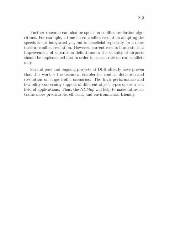
213
Further research can also be spent on conflict resolution algo-rithms. For example, a time-based conflict resolution adapting thespeeds is not integrated yet, but is beneficial especially for a moretactical conflict resolution. However, current results illustrate thatimprovement of separation definitions in the vicinity of airportsshould be implemented first in order to concentrate on real conflictsonly.
Several past and ongoing projects at DLR already have proventhat this work is the technical enabler for conflict detection andresolution on huge traffic scenarios. The high performance andflexibility concerning support of different object types opens a newfield of applications. Thus, the NDMap will help to make future airtraffic more predictable, efficient, and environmental friendly.

214 CHAPTER 7. CONCLUSIONS AND OUTLOOK
Chapter 8Update after Disputation
Since the disputation took place ∼18 months after submission ofthis thesis, several work proposed in the outlook already has beenperformed when passing to press. Because most of the new featuresconfirm the high value of the presented algorithms, this chaptergives a brief summary on what has been achieved since submission.
8.1 Conflict Metric
The conflict metric has been extended to cover parallel runway con-figurations for approach mode as defined in section 2.4. Furthermore,the dynamic wake turbulence separation has been implemented.As a result, it was possible with the presented conflict resolutionalgorithms to get the European scenario free of conflict.
Since resolution of the European scenario worked very well, Ifurthermore extended the separation requirements from 5 NM to6.5 NM, 8 NM, 10 NM, and even 12 NM. The idea was to use thewell known 5 NM as safety separation, and leave the remainingspace for allowed deviations from the trajectory. These alloweddeviations may be used pro-actively by the aircraft to optimize the
215

216 CHAPTER 8. UPDATE AFTER DISPUTATION
trajectory furthermore. They also give freedom when deviationsoccur, e. g., due to a bad weather forecast.
Even with the increased separation requirements, generationof a conflict free traffic scenario was always possible. Resultsare summarized in table 8.1. The last three rows hold necessaryadaptations to get the optimized scenario resolved:
• The average Time Shift describes the average absolute timeshift each aircraft was shifted from its initial departure time;
• The average Add. Climb specifies how many extra feet eachaircraft has to climb compared to its initial route on average;
• The average Add. Dist states how many extra distance eachaircraft has to fly compared to its initial route on average.
More detailed information is available from Kuenz (2014).
Table 8.1 – Results from Trials with Increased Separation
Scenario
5 NM 6.5 NM 8 NM 10 NM 12 NM
Separation 5 NM 6.5 NM 8 NM 10 NM 12 NMFreedom 0 NM 0.75 NM 1.5 NM 2.5 NM 3.5 NMConflicts 24 162 28 328 33 115 40 562 48 942
En-Route 11 137 15 303 20 088 27 534 35 912Airport 13 025 13 025 13 027 13 028 13 030
Time Shift 93.9 s 120.8 s 143.4 s 192.2 s 200.2 sAdd. Climb 16.9 ft 40.8 ft 59.8 ft 159.2 ft 220.0 ftAdd. Dist. 3.7 m 68 m 137 m 1.3 NM 3.5 NM
8.2 Performance
Improved data structures have been integrated in the algorithmespecially increasing the conflict detection speed for large scenarios.New links from objects to their conflicts increase coordination effort

8.2. PERFORMANCE 217
0
10
20
30
40
50
60
70
80
90
0 5 10 15 20 25 300
0.5
1
1.5
2
2.5
3
3.5
4
4.5To
talC
onfli
ctD
etec
tion
Tim
e(s)
Mem
ory
Usa
ge(G
B)
Number of Trajectories in Thousand
Detection TimeMemory Usage
Figure 8.1 – Improved Detection Times with New Data Structuresfor Europe
slightly only, but increase significantly the speed to validate if theconflict already exists. Furthermore, hash maps were added to findobjects much quicker than before. Figure 8.1 shows the increasedspeed of the NDMap with improved data structures. With about82 s the algorithm halves the original detection time. Even for thesmaller German traffic sample, the NDMap performs about 20 %better, compare fig. 8.2.

218 CHAPTER 8. UPDATE AFTER DISPUTATION
0
2
4
6
8
10
12
14
0 2000 4000 6000 8000 100000
0.1
0.2
0.3
0.4
0.5
0.6
0.7
0.8
Tota
lCon
flict
Det
ecti
onT
ime(
s)
Mem
ory
Usa
ge(G
B)
Number of Trajectories
Detection TimeMemory Usage
Figure 8.2 – Improved Detection Times with New Data Structuresfor Geramy

Bibliography
Abam, M., M. Berg, S.-H. Poon, and B. Speckmann (2006). Ki-netic collision detection for convex fat objects. In Y. Azar andT. Erlebach (Eds.), Algorithms - ESA 2006, Volume 4168, pp.4–15. Springer Berlin Heidelberg.
Adam, V. and R. Kohrs (1992). On board planning of 4D-trajectories. AGARD CP 504, 16.1–16.12.
Basch, J., J. Erickson, L. J. Guibas, J. Hershberger, and L. Zhang(1999). Kinetic collision detection between two simple polygons.In Proceedings of the Tenth Annual ACM-SIAM Symposium onDiscrete Algorithms, SODA ’99, Philadelphia, PA, USA, pp. 102–111. Society for Industrial and Applied Mathematics.
Beckmann, N., H. P. Kriegel, R. Schneider, and B. Seeger (1990).The r*-tree: an efficient and robust access method for points andrectangles. In Proceedings of the 1990 ACM SIGMOD interna-tional conference on Management of data - SIGMOD ’90, pp.322.
Bentley, J. L. (1975). Multidimensional binary search trees usedfor associative searching. Communications of the ACM 18(9),509–517.
219

220 BIBLIOGRAPHY
Bentley, J. L. and T. A. Ottmann (1979). Algorithms for reportingand counting geometric intersections. IEEE Transactions onComputers C-28 (9), 643–647.
Birkmeier, B., B. Korn, and D. Kügler (2010, October). SectorlessATM and advanced SESAR concepts: Complement not contra-diction. In 29th Digital Avionics Systems Conference.
Bode, S. and P. Hecker (2013, August). Efficient 4D trajectoryconflict detection for large scale atm simulations using bounding-volume hierarchies and time-spatial indexing. In Proceedings of theAIAA Modeling and Simulation Technologies (MST) Conference.
Boehm, B. (1979). Guidelines for verifying and validating softwarerequirements and design specifications. In Euro IFIP 79.
Boguhn, O. (2007). Internal Project Leiser Flugverkehr II. Technicalreport, Institute of Aerodynamics and Flow Technology, DLRGöttingen.
Central Intelligence Agency (2007). The CIA World Factbook.United States.
Chazelle, B. (1988). A functional approach to data structures andits use in multidimensional searching. SIAM J. Comput. 17,427–462.
Chazelle, B. (1991). Triangulating a simple polygon in linear time.Discrete & Computational Geometry 6, 485–524.
Cohen, J. D., M. C. Lin, D. Manocha, and M. Ponamgi (1995).I-collide: An interactive and exact collision detection system forlarge-scale environments. In In Proc. of ACM Interactive 3DGraphics Conference, pp. 189–196.
Coming, D. S. and O. G. Staadt (2005). Kinetic sweep and prunefor collision detection. In F. Ganovelli and C. Mendoza (Eds.),Workshop On Virtual Reality Interaction and Physical Simulation.
Czerlitzki, B. (1994). The experimental flight management system:Advanced functionality to comply with atc constraints. Air TrafficControl Quarterly Vol. 2(3), 159–188.

BIBLIOGRAPHY 221
Czerlitzki, B. and R. Kohrs (1994). 4D Flight Management -Planungsfunktionen zur Einhaltung von Zeitvorgaben. ZFW- Zeitschrift für Flugwissenschaften und Weltraumforschung 18,Heft 1, 40–47.
de Muynck, R., T. Bos, A. Kuenz, C. Edinger, L. Rappich, andS. Törner (2011). Real time ATC simulation of time based CDAoperations. In CEAS 2011.
Deutsches Institut für Normierung (1999, Oct). DIN ISO 9613-2:Dämpfung des Schalls bei der Ausbreitung im Freien.
DFS Deutsche Flugsicherung (2011). Luftverkehr in Deutschland -Mobilitätsbericht 2011.
Dobkin, D. P. and D. G. Kirkpatrick (1983). Fast detection ofpolyhedral intersection. Theroretical Computer Science 27, 241–253.
Douglas, D. and T. Peucker (1973). Algorithms for the reductionof the number of points required to represent a digitized line orits caricature. The Canadian Cartographer 10(2), 112–122.
Dougui, N., D. Delahaye, S. Puechmorel, and M. Mongeau (2010).A new method for generating optimal conflict free 4D trajectory.Proc 4th International Conference on Research in Air Transporta-tion 4, 185–191.
Duong, V., E. Hoffman, L. Floc’hic, J.-P. Nicolaon, and A. Bossu(1996). Extended flight rules (EFR) to apply to resolution ofencounters in autonomous airborne separation. http://www.asas-tn.org/library/asassworksdonesbysrdsbod/freer/freer/rules-02.pdf (March 2013), Boston.
Durand, N., J.-M. Alliot, and J. Noailles (1996). Automatic aircraftconflict resolution using genetic algorithms. In Proceedings ofthe 1996 ACM symposium on Applied Computing, SAC ’96, NewYork, NY, USA, pp. 289–298. ACM.
Dworkin, P. and D. Zeltzer (1993). A new model for efficientdynamic simulation. In Proceedings of the Eurographics Workshopon Animation and Simulation, pp. 135–147.

222 BIBLIOGRAPHY
Edelsbrunner, H. and H. A. Maurer (1981). On the intersection oforthongonal objects. Information Processing Letters 13, 177–181.
Ericson, C. (2005). Real Time Conflict Detection. Morgan Kauf-mann.
Erzberger, H., T. A. Lauderdale, and Y.-C. Chu (2010). Automatedconflict resolution, arrival management and weather avoidancefor atm. In 27th Congress of the Internation Council of theAeronautical Sciences, Volume 27.
Erzberger, H., R. A. Paielli, D. R. Isaacson, and M. M. Eshow(1997). Conflict detection and resolution in the presence ofprediction error. In Proc. 1st USA/Eur. Air Traffic Manage. Res.Development Seminar, pp. 50–56.
Eurocontrol (2010). DDR reference manual. http://www.eurocontrol.int/services/demand-data-repository-ddr (Jan.2013).
Eurocontrol (2011). Base of aircraft data (BADA) version 3.9.http://www.eurocontrol.int/eec/public/standard_page/proj_BADA.html (Jan. 2013).
Eurocontrol (2012). Airborne collision avoidance system ii. http://www.eurocontrol.int/dossiers/acas-ii (Jan. 2013).
Federal Aviation Administration (2012). Implementation plan.http://www.faa.gov/nextgen/media/ng2011_implementation_plan.pdf (Jan. 2013).
Federal Aviation Administration (2013). Next generation air trans-portation system. http://www.faa.gov/nextgen (Jan. 2013).
Foudil, C., D. Noureddine, C. Sanza, and Y. Duthen (2009). Pathfinding and collision avoidance in crowd simulation. In Journalof Computing and Information Technology.
Fuchs, H., Z. M. Kedem, and B. F. Naylor (1980). On visiblesurface generation by a priori tree structures. In SIGGRAPH ’80Proceedings of the 7th annual conference on Computer graphicsand interactive techniques, pp. 124–133.

BIBLIOGRAPHY 223
Fuller, B. (1943, March). Life Presents R. Buckminster Fuller’sDymaxion World, pp. 41–55. Henry Luce.
Gargantini, I. (1982). Linear octrees for fast processing of three-dimensional objects. Computer Graphics and Image Processing 20,365–374.
Geister, D. (2012). Constraint Generierung für domänenspezifis-che Modellierungssprachen. Ph. D. thesis, Leibniz UniversitätHannover.
Golas, A., R. Narain, S. Curtis, and M. C. Lin (2013). Hybrid long-range collision avoidance for crowd simulation. IEEE Transactionson Visualization and Computer Graphics 1, 29–36. Early Access.
Guibas, L. J. (2001). Kinetic data structures. In Chapman andHall/CRC (Eds.), Handbook of Data Structures and Applications,pp. 23–1–23–18. Mehta, Dinesh P.; Sahni, Sartaj.
Guttman, A. (1984). R-trees: A dynamic index structure for spatialsearching. In SIGMOD ’84 Proceedings of the 1984 ACM SIG-MOD international conference on Management of data, Volume1984, pp. 47–57.
Hart, P. E., N. J. Nilsson, and B. Raphael (1968). A formal basisfor the heuristic determination of minimum cost paths. 4 (2),100–107.
Hildum, D. W. and S. F. Smith (2004). Scheduling safe movementof air traffic in crowded air spaces. The Knowledge EngineeringReview 27, 309–331.
Hopcroft, J. E., J. Schwartz, and M. Sharir (1983). Efficient detec-tion of intersections among spheres. Internat. J. Robot Res. 2,77–80.
Houthuys, P. (1987). Box sort, a multidimensional binary sortingmethod for rectangular boxes, used for quick range searching.The Visual Computer 3, 236–249.
ICAO (2002). Annex 10 to the convention on international civilaviation: Aeronautical telecommunications. Technical report,International Civil Aviation Organization.

224 BIBLIOGRAPHY
ICAO (2004a). Annex 14 to the convention on international civil avi-ation: Aerodromes. Technical report, International Civil AviationOrganization.
ICAO (2004b). Doc 9643: Manual on simultaneous operations onparallel or near-parallel instrument runways (SOIR). Technicalreport, International Civil Aviation Organization.
ICAO (2005). Doc 9854: Global air traffic management opera-tional concept. Technical report, International Civil AviationOrganization.
ICAO (2007). Doc 4444: Air traffic management. Technical report,International Civil Aviation Organization.
ICAO (2008). Guidance on A380-800 wake vortex aspects. Technicalreport, International Civil Aviation Organization.
Jardin, M. (2003). Real-time conflict-free trajectory optimization.In 5th USA/Europe ATM R&D Seminar.
Jardin, M. (2005). Grid-based strategic air traffic conflict detection.In AIAA Guidance, Navigation, and Control Conference andExhibit, San Francisco, California.
Jeck, R. K. (2002). Icing design envelopes (14 cfr parts 25 and29, appendix c) converted to a distance-based format. Technicalreport, Federal Aviation Administration.
jen Chiang, Y., J. T. Klosowski, C. Lee, and J. S. B. Mitchell(1997). Geometric algorithms for conflict detection/resolutionin air traffic management. In Proceedings of the 36th IEEEConference on Decision and Control, Volume 2, pp. 1835–1840.
Joulia, A. and C. Le Tallec (2012). Aircraft 4D contract basedoperation: The 4DCo-GC project. In 28th Congress of the Inter-national Council of the Aeronautical Sciences.
Kelly, M., K. Gould, B. Pease, S. Winner, and A. Yen (1994).Hardware accelerated rendering of CSG and transparency. InSIGGRAPH’94 Proceedings of the 21st anual conference on Com-puter graphics and interactive techniques, pp. 177–184.

BIBLIOGRAPHY 225
Kelly, W. E. and M. S. Eby (2000). Advances in force field con-flict resolution algorithms. In AIAA Guidance, Navigation andControl Conference and Exhibit.
Klosowski, J. T., M. Held, J. S. B. Mitchell, H. Sowizral, andK. Zikan (1998). Efficient collision detection using boundingvolume hierarchies of k-dops. 4 (1), 21–36.
Koeners, J. and M. de Vries (2008). Conflict resolution support forair traffic control based on solution spaces: Design and imple-mentation. In Proc. IEEE/AIAA 27th Digital Avionics SystemsConf. DASC 2008.
Kohrs, R. (1992). Planung von 4D-Trajektorien an Bord einesFlugzeugs. DGLR Jahrbuch 2, 943–952.
Korn, B., C. Edinger, S. Tittel, D. Kügler, T. Putz, O. Hassa, andB. Mohrhard (2009). Sectorless ATM — a concept to increaseen-route efficiency. In Proc. IEEE/AIAA 28th Digital AvionicsSystems Conf. DASC 2009.
Korn, B. and A. Kuenz (2006, Oktober). 4D FMS for increasingefficiency of TMA operations. In Proc. IEEE/AIAA 25th DigitalAvionics Systems Conf. DASC 2006.
Kremer, H., W. Vertegaal, and R. Jansen (1999). Phare advancedtools conflict probe - final report. Technical report, Programmefor Harmonised ATM Research in EUROCONTROL.
Kuenz, A. (2011). A global airspace model for 4D-trajectory-basedoperations. In Proc. IEEE/AIAA 30th Digital Avionics SystemsConf. DASC 2011.
Kuenz, A. (2012, Juni). Optimizing tomorrows ATM using 4D-trajectory-based operations. In ODAS 2012.
Kuenz, A. (2014). Increasing the margins - more freedom intrajectory-based operations. In Proc. IEEE/AIAA 33rd Dig-ital Avionics Systems Conf. DASC 2014.
Kuenz, A., H. Becker, C. Edinger, and B. Korn (2008, Septem-ber). Performance-based TMA handling for mixed traffic using

226 BIBLIOGRAPHY
a ground based 4D-guidance for unequipped aircraft. In 26thICAS Congress (Ed.), 26th Congress of the International Councilof the Aeronautical Sciences, Number 26 in ICAS.
Kuenz, A. and C. Edinger (2010a, September). Future air groundintegration: A scalable concept to start with green approachestoday. In 27th Congress of the Internation Council of the Aero-nautical Sciences.
Kuenz, A. and C. Edinger (2010b, Oktober). Green approacheswithout trade-off: Final results from the FAGI-project. In Proc.IEEE/AIAA 29th Digital Avionics Systems Conf. DASC 2010.
Kuenz, A., V. Mollwitz, and B. Korn (2007, Oktober). Greentrajectories in high traffic TMAs. In Proc. IEEE/AIAA 26thDigital Avionics Systems Conf. DASC 2007.
Kuenz, A. and N. Peinecke (2009, Oktober). Tiling the world -efficient 4D conflict detection for large scale scenarios. In Proc.IEEE/AIAA 28th Digital Avionics Systems Conf. DASC 2009,Volume 28 of DASC Conference.
Kuenz, A. and N. Peinecke (2011, February). Effiziente 4D-Konflikt-Erkennung für großräumige Szenarien, Verfahren zur Ermittlungeiner potenziellen Konfliktsituation. Patent (EP 2 457 224 A2).
Kuenz, A. and N. Peinecke (2012, June). Method for determininga potential conflict situation. Patent (US20120158278).
Kuenz, A. and G. Schwoch (2012). Global time-based conflictsolution towards the overall optimium. In Proc. IEEE/AIAA31st Digital Avionics Systems Conf. DASC 2012.
Kuenz, A., G. Schwoch, and F.-E. Wolter (2013). Individualism inglobal airspace - user-preferred trajectories in future ATM. InProc. IEEE/AIAA 32nd Digital Avionics Systems Conf. DASC2013.
Lewis, G. N., N. J. Boynton, and F. W. Burton (1981). Expectedcomplexity of fast search with uniformly distributed data. Inform.Proc. Let. 13, 4–7.

BIBLIOGRAPHY 227
Manolopoulos, Y., A. Nanopoulos, and Y. Theodoridis (2006).R-trees: Theory and applications. Springer. ISBN 978-1-85233-977-7 1, 15–34.
Mount, D. M. (1997). Geometric intersection. In J. E. Goodmanand J. O’Rourke (Eds.), Handbook of Discrete and ComputationalGeometry (2 ed.)., Chapter 38, pp. 857–876. CRC Press LLC,Boca Raton, FL.
Naylor, B. (1993, May). Constructing good partitioning trees. InGraphics Interface (annual Canadian CG conference).
Osborne, P. (2008). The mercator projections. Technical report,University of Edingburgh, Edinburgh.
Popper, K. (1974). Autobiography: The philosophy of Karl Popper,Volume Abschnitt 8. P. A. Schilpp.
Prautzsch, H., W. Boehm, and M. Paluszny (2002). Bezier- andB-spline techniques. Springer.
Ramer, U. (1972). An iterative procedure for the polygonal ap-proximation of plane curves. Computer Graphics and ImageProcessing 1, 244–256.
Reichling, M. (1988). On the detection of a common intersection ofk convex objects in the plane. Informa. Process. Lett. 29, 25–29.
Rosenberg, J. (1985). Geographical data structures compared:A study of data structures supporting region queries. IEEETransaction on CAD Integrated Circuits Systems 4(1), 53–67.
Roussos, G. P., G. Chaloulos, K. J. Kyriakopoulos, and J. Lygeros(2008). Control of multiple non-holonomic air vehicles underwind uncertainty using model predictive control and decentralizednavigation functions. In Proc. 47th IEEE Conf. Decision andControl CDC 2008, pp. 1225–1230.
Samet, H. (1990). The Design and Analysis of Spatial Data Struc-tures. Addison-Wesley.

228 BIBLIOGRAPHY
Schlager, H., H. Mannstein, B. Weinzierl, F. Linke, and T. Mühl-hausen (2012). Projektplan volcanic ash impact on the air trans-port system. Project plan.
Schumacker, R. A., B. Brand, M. G. Gilliland, and W. H. Sharp(1969). Study for applying computer-generated images to visualsimulation. Technical report, U.S. Air Force Human ResourcesLaboratory.
Schwoch, G. (2008, June). Konflikterkennung und -lösung in zukün-ftigen Luftfahrtszenarien basierend auf 4D-Flugbahnen. Technicalreport, Technische Universität Braunschweig.
SESAR Consortium (2007). The ATM target concept D3. Technicalreport, SESAR Consortium.
SESAR Consortium (2008). Sesar master plan D5. Technical report,SESAR Consortium.
SESAR Consortium (2010). Sesar brochure: Modernising the euro-pean sky. Technical report, SESAR Consortium.
SESAR Joint Undertaking (2013). Sesar. http://www.sesarju.eu (Jan. 2013).
Shamos, M. I. and D. Hoey (1976). Geometric intersection problems.In Proc. th Annual Symp. Foundations of Computer Science, pp.208–215.
Smedt, D. D. and G. Berz (2007). Study of the required time ofarrival function of current FMS in an ATM context. In Proc.IEEE/AIAA 26th Digital Avionics Systems Conf. DASC 2007.
Smith, S. F. (2008). Constraint-based techniques for managingmovement in crowded airspaces. In 7th INO Workshop.
Snyder, J. P. (1987). Map projections: A working manual. USGSProfessional Paper 1395, 243–248.
Stell, L. (2010). Analysis of flight management system predictions ofidle-thrust descents. In Proc. IEEE/AIAA 29th Digital AvionicsSystems Conf. DASC 2010.

BIBLIOGRAPHY 229
Tavares, D. L. M. and J. L. D. Comba (2007). Broad-phase col-lision detection using delaunay triangulation. Technical report,Universidade Federal do Rio Graqnde do Sul (UFRGS).
Teschner, M., B. Heidelberger, M. Mueller, D. Pomeranets, andM. Gross (2003). Optimized spatial hashing for collision detectionof deformable objects. In Proceedings of the Vision, Modeling,and Visualization Conference, pp. 47–54.
Teschner, M., S. Kimmerle, B. Heidelberger, G. Zachmann,L. Raghupathi, A. Fuhrmann, M.-P. Cani, F. Faure, N. Magnenat-Thalmann, W. Strasser, and P. Volino (2005). Collision detectionfor deformable objects. In Computer Graphics Forum, Volume 24,pp. 61–81.
The 4DCo-GC Consortium (2013). 4DCo-GC project. http://www.4dcogc-project.org/ (Jul. 2013).
The CGAL Project (2015). CGAL User and Reference Manual(4.6.1 ed.). CGAL Editorial Board.
Vincenty, T. (1975). Direct and inverse solutions of geodesics on theellipsoid with application of nested equations. In Survey Review,Volume XXIII.
Voggenreiter, H. and W. Etzenbach (2012). DLR@UNI - Die insti-tutionalisierte Zusammenarbeit zwischen DLR und Universitäten.9-22.
Vujasinovic, R. (2012a). ATM and volcanic ash: An advanced ap-proach to adverse event. In International Conference on Researchin Air Transportation - ICRAT, Volume 5.
Vujasinovic, R. (2012b). Volcanic ash events: When the role ofdecision maker is assigned to a pilot. In Proc. of Integrated Com-munications Navigation and Suerveillance (ICNS) Conference.
Wald, I. and V. Havran (2006). On building fast kd-trees for raytracing, and on doing that in O(NlogN). In In Proceedings of the2006 IEEE Symposium on interactive ray tracing, pp. 61–70.

230 BIBLIOGRAPHY
Woo, M., J. Neider, T. Davis, and D. Shreiner (1999). OpenGLProgramming Guide: The Official Guide to Learning OpenGL,Version 1.2 (3rd ed.). Boston, MA, USA: Addison-Wesley Long-man Publishing Co., Inc.
Zachmann, G. (1998). Rapid collision detection by dynamicallyaligned dop-trees. In Proceedings of Virtual Reality Annual In-ternational Symposium, Atlanta, GA, USA, pp. 90–97.
Zachmann, G. and R. Weller (2006). Kinetic bounding volumehierarchies for deformable objects.

Index
4D-Trajectory, 244DCo-GC, 168
Affected Tiles, 92Aircraft Related Restrictions, 46Airport-Focused Conflict Prob-
ing, 187Alternative Earth Mapping, 134Aviation Conflicts, 59
Bézier Curves, 39Balancing, 102Binary Tree, 28Bounding Boxes, 38, 99Bounding Volume Hierarchy, 38Broad Phase, 33, 104BSP, 28
Comparison with Octrees, 159Complex Scenarios, 33Conclusions and Outlook, 209Conflict Detection, 81Conflict Detection in 4D-
Airspace, 125Conflict Detection Mechanisms,
32Conflict Resolution, 171
Conflict-Jitter, 198Continuous Motion, 33Convex Polygon, 34Crowd Simulation, 72
Date Line, 131, 202Definitions, 83Delauney Triangulation, 44Detection, 81Discontinuity, 131, 202Discrete Motion, 33Douglas Peucker Algorithm, 130
Earth-Mode, 126Earth-Shape Support, 126European Traffic Sample, 139Extended Flight Rules, 73
FAGI, 161Flight Duration, 183Focus Objects, 121Focus on Aircraft, 156Full Containment, 98
Gauss-Krüger, 78Geodesic Dome, 136Geodetic Earth Systems, 73
231

232 INDEX
German Traffic Sample, 137Global Conflict Probing, 188Global Shifting Algorithm, 180Great Circle Connections, 129
Hashing, 44Hyperrectangle, 90
Intersection Searching, 37Introduction, 23
k-d tree, 30Key Performance Areas, 172Kinetic Data Structures, 41
Lateral Resolution, 175Lateral Resolution Probing, 190Lateral Tile Size Optimization,
149Light Propagation, 72Line Segment, 83Luftraummanagement 2020, 163
Mathematics and Algorithms, 27Memory Limitation, 105Mercator Projection, 77Merging of Conflicts, 118
N-Dimensional Conflict Detec-tion, 113
N-Dimensional Conflicts, 87N-Dimensional Moving Polygon
Volumes, 109N-Dimensional Polygon Vol-
umes, 107N-Dimensional Trajectories, 106Narrow Phase, 33, 104Nominal Case, 194
Object, 85
Penetration, 93Performance Indicators, 145Performance Optimization for
CD, 148Plane Sweep, 36Poles, 131, 201Polygon Volume, 205Potential Fields, 71Pseudo-Parallel Trajectories, 194
R-tree, 30Ramer Algorithm, 130Range Searching, 37Recursion, see RecursionRecursive Shifting Algorithm,
181Related Work, 27Resolution, 171Results from Conflict Detection,
141Right of Way, 73Root Tile, 157
Sectorless ATM, 163Simple Polygon, 35Simplex, 85Singularity, 131, 201Sinusoidal Projection, 77Spatial Hashing, 44Spatial Subdivision, 44Suladi, 167Supported Objects, 106Sweep and Prune, 43Sweepline, 36Symmetric Simplification, 97
Tesseract, 90Tile Knowledge, 105Tiling Algorithm, 89
INDEX 233
Time-Based Resolution, 178Time-based Tile Size Optimiza-
tion, 151Time-Shift, 179Traffic Samples and Conditions,
137Trajectory, 83Trajectory Prediction, 46Transverse Mercator projection,
78Trial-and-Error, 172Triangulation, 44
Validation, 193Verification, 193Vertical Resolution, 177Vertical Resolution Probing, 190Vertical Tile Size Optimization,
149Vicinity, 95Volume, 86

234
Lebenslauf
Name Dipl.-Inform. Alexander Kuenz
Anschrift In den Grashöfen 5038110 BraunschweigTelefon Beruf: (0531) 295 [email protected]
Geburtsdatum und -ort08. 09. 1974 in Bad Harzburg
Familienstandverheiratet, ein Sohn (� 2008) und eine Tochter(� 2014)
Ausbildung8/1981-6/1994 Schulausbildung, Abitur am Werner-von-Sie-
mens Gymnasium Bad Harzburg
9/1994-3/1997 Ausbildung zum Mathematisch-Technischen As-sistenten (MaTA) beim DLR Braunschweig
3/1997-10/1997 Arbeit als MaTA beim DLR Braunschweig
10/1997-10/2001 Informatikstudium an der Technischen Universi-tät Braunschweig mit der Gesamtnote sehr gut
Studienschwerpunkte: Theoretische Infor-matik, Rechnerstrukturen, Telematik, Da-tenbanken, Signalverarbeitung
Studienarbeit: Entwicklung einer Client/Server-Applikation für eine Navigations-datenbasis

235
Diplomarbeit: An Architectural Model forHeterogeneous Hardware/Software Plat-forms
Berufliche Erfahrung10/1997-10/2001 Studienbegleitende Arbeit am Institut für Flug-
führung, DLR Braunschweig, Abteilung Anthro-potechnik und Simulation
seit 11/2001 Wissenschaftlicher Mitarbeiter in der Abteilungfür Pilotenassistenz
2001-2004 Mitarbeit an den Projekten ASSIST, ATTASUpgrade und Wasla Hale
2004-2007 Arbeitspaketleitung im DLR-internen ProjektLeiser Flugverkehr II
2005-2008 Arbeitspaketleitung im BMBF-Projekt LeiseAn- und Abflüge (LAnAb) im Forschungsver-bund Leiser Verkehr
2007-2009 Projektleitung des DLR-internen Projektes Fu-ture Air Ground Integration (FAGI)
2007-2009 Verantwortung für die Arbeitsanteile des Insti-tuts für Flugführung am DLR-internen ProjektFuture Aeronautical Communications TrafficSimulator (FACTS)
2007-2011 Projektleiter des DLR-Anteils im FP6-ProjektEnvironmentally Responsible Air Transport(ERAT)
2007-2009 Mitarbeit im europäischen Trajectory Predicti-on Gremium
seit 2008 Dozent bei CCG-Seminaren
2010-2013 Projektleiter des DLR-Anteils und Leiter desArbeitspakets Integration im FP7-Projekt4 Dimensional-Contracts - Guidance and Con-trol (4DCo-GC)

236
seit 2011 Projektleiter für die Arbeitsanteile des Institutsfür Flugführung im HGF-Projekt SupercooledLarge Droplets Icing (SuLaDI)
SprachkenntnisseEnglisch fließend in Wort und Schrift
Grundkenntnisse in Französisch, Spanisch undItalienisch
FortbildungenScientific Skills z.B. Noise Abatement Procedures Workshop
GBAS-WorkshopWakeNet WorkshopGate-to-Gate Open DaysCourage Trajectory Prediction WorkshopGenspace-Workshop (Lotsentraining)BZF und AZF FunksprechzeugnisseTeilnahme an und Beiträge zu diversen Konfe-renzen
Soft Skills z.B. Moderation von GesprächsrundenVerständliche und überzeugende Gesprächsfüh-rung mit Kollegen und KundenIntensivkurs Projektmanagement
Braunschweig, 21. September 2015