high angle-of-attack flight characteristics of a small uav
TRANSCRIPT

HIGH ANGLE-OF-ATTACK FLIGHT CHARACTERISTICS OF A SMALL UAV WITHA VARIABLE-SIZE VERTICAL TAIL
By
BARON JON JOHNSON
A THESIS PRESENTED TO THE GRADUATE SCHOOLOF THE UNIVERSITY OF FLORIDA IN PARTIAL FULFILLMENT
OF THE REQUIREMENTS FOR THE DEGREE OFMASTER OF SCIENCE
UNIVERSITY OF FLORIDA
2009
1

c© 2009 Baron Jon Johnson
2

I dedicate this to my loving parents, who have fully supported my every endeavor, and to
Michael Morton, a dear friend, roommate, and colleague who was taken far too early.
You will always be missed Morty.
3

ACKNOWLEDGMENTS
I would like to extend thanks to a number of supportive and inspiring people with
whom I’ve had the honor, privilege, and pleasure to work with during my time at the
University of Florida. First of all, thanks to my advisor, Dr. Rick Lind, for providing me
the opportunity to study under him during graduate school in the Flight Control Lab.
His guidance, suggestions, and critiques have proven invaluable. Thanks to Dr. Peter
Ifju for offering me the most exciting and rewarding job I could have ever imagined as an
undergraduate in the Micro Air Vehicle Lab.
A number of fellow students have also supported me in my time at UF, either directly
or indirectly. Scott Bowman has always provided a great deal of support and made
great contributions to my understanding of electronic systems, particularly in the field of
shooting bottle rockets from RC planes. Assistance, inspiration, and constant amusement
has been provided by the current members of the Flight Control Lab, listed in a very
particular order: Dong Tran, Sanketh Bhat, Daniel ’Tex’ Grant, Robert Love, Brian
Roberts, and Ryan Hurley. Other collaborators which have made strong impressions upon
me over the years include Mujahid Abdulrahim, Carlo Francis, Frank Boria, Dan Claxton,
Kyuho Lee, Adam Watts, Jos Cocquyt, and Patricia Miller.
4

TABLE OF CONTENTS
page
ACKNOWLEDGMENTS . . . . . . . . . . . . . . . . . . . . . . . . . . . . . . . . . 4
LIST OF TABLES . . . . . . . . . . . . . . . . . . . . . . . . . . . . . . . . . . . . . 7
LIST OF FIGURES . . . . . . . . . . . . . . . . . . . . . . . . . . . . . . . . . . . . 8
ABSTRACT . . . . . . . . . . . . . . . . . . . . . . . . . . . . . . . . . . . . . . . . 10
CHAPTER
1 INTRODUCTION . . . . . . . . . . . . . . . . . . . . . . . . . . . . . . . . . . 12
1.1 High Angle-of-Attack Flight . . . . . . . . . . . . . . . . . . . . . . . . . . 121.2 Motivation . . . . . . . . . . . . . . . . . . . . . . . . . . . . . . . . . . . . 131.3 Previous Research . . . . . . . . . . . . . . . . . . . . . . . . . . . . . . . . 131.4 Contributions . . . . . . . . . . . . . . . . . . . . . . . . . . . . . . . . . . 16
2 EXPERIMENTAL SETUP . . . . . . . . . . . . . . . . . . . . . . . . . . . . . 17
2.1 Aircraft . . . . . . . . . . . . . . . . . . . . . . . . . . . . . . . . . . . . . 172.2 Vertical Tail . . . . . . . . . . . . . . . . . . . . . . . . . . . . . . . . . . . 182.3 Avionics . . . . . . . . . . . . . . . . . . . . . . . . . . . . . . . . . . . . . 19
3 FLIGHT TESTING . . . . . . . . . . . . . . . . . . . . . . . . . . . . . . . . . 25
4 ANALYSIS TECHNIQUES . . . . . . . . . . . . . . . . . . . . . . . . . . . . . 28
4.1 Fourier Transform . . . . . . . . . . . . . . . . . . . . . . . . . . . . . . . . 284.2 Wavelet Transform . . . . . . . . . . . . . . . . . . . . . . . . . . . . . . . 284.3 Examples . . . . . . . . . . . . . . . . . . . . . . . . . . . . . . . . . . . . 30
4.3.1 Example 1: Stationary Sine Wave Signal . . . . . . . . . . . . . . . 304.3.2 Example 2: Stationary Signal with Multiple Frequency Components 314.3.3 Example 3: Chirp Signal with Increasing Frequency . . . . . . . . . 33
5 SYSTEM IDENTIFICATION . . . . . . . . . . . . . . . . . . . . . . . . . . . . 36
5.1 Procedure . . . . . . . . . . . . . . . . . . . . . . . . . . . . . . . . . . . . 365.2 Doublet Modeling . . . . . . . . . . . . . . . . . . . . . . . . . . . . . . . . 38
5.2.1 Longitudinal . . . . . . . . . . . . . . . . . . . . . . . . . . . . . . . 385.2.2 Lateral . . . . . . . . . . . . . . . . . . . . . . . . . . . . . . . . . . 405.2.3 Directional . . . . . . . . . . . . . . . . . . . . . . . . . . . . . . . . 41
5.3 Steady-State Flight . . . . . . . . . . . . . . . . . . . . . . . . . . . . . . . 435.3.1 Longitudinal . . . . . . . . . . . . . . . . . . . . . . . . . . . . . . . 435.3.2 Lateral . . . . . . . . . . . . . . . . . . . . . . . . . . . . . . . . . . 455.3.3 Directional . . . . . . . . . . . . . . . . . . . . . . . . . . . . . . . . 47
5

6 VERTICAL TAIL RELATIONSHIP TO WING ROCK . . . . . . . . . . . . . . 50
6.1 Upright Tail . . . . . . . . . . . . . . . . . . . . . . . . . . . . . . . . . . . 506.2 Inverted Tail . . . . . . . . . . . . . . . . . . . . . . . . . . . . . . . . . . . 526.3 Parameterization . . . . . . . . . . . . . . . . . . . . . . . . . . . . . . . . 56
7 SUMMARY . . . . . . . . . . . . . . . . . . . . . . . . . . . . . . . . . . . . . . 62
7.1 Recommendations . . . . . . . . . . . . . . . . . . . . . . . . . . . . . . . . 627.2 Conclusion . . . . . . . . . . . . . . . . . . . . . . . . . . . . . . . . . . . . 63
REFERENCES . . . . . . . . . . . . . . . . . . . . . . . . . . . . . . . . . . . . . . . 65
BIOGRAPHICAL SKETCH . . . . . . . . . . . . . . . . . . . . . . . . . . . . . . . . 69
6

LIST OF TABLES
Table page
2-1 Mini ShowTime Specifications . . . . . . . . . . . . . . . . . . . . . . . . . . . . 18
2-2 Mini ShowTime Components . . . . . . . . . . . . . . . . . . . . . . . . . . . . 18
2-3 Vertical Tail Specifications . . . . . . . . . . . . . . . . . . . . . . . . . . . . . . 19
2-4 Size and Mass of Avionics . . . . . . . . . . . . . . . . . . . . . . . . . . . . . . 20
2-5 IMU/FDR Wiring Sequence . . . . . . . . . . . . . . . . . . . . . . . . . . . . . 22
2-6 Technical Specifications of IMU Sensors . . . . . . . . . . . . . . . . . . . . . . 23
2-7 IMU Raw Output Multipliers and Resulting Units . . . . . . . . . . . . . . . . . 24
7

LIST OF FIGURES
Figure page
1-1 Graphical Representation of Angle-of-Attack . . . . . . . . . . . . . . . . . . . . 12
1-2 F/A-18 HARV and X-29 . . . . . . . . . . . . . . . . . . . . . . . . . . . . . . . 14
1-3 RQ-11B Raven Small Unmanned Aircraft System . . . . . . . . . . . . . . . . . 15
2-1 Mini ShowTime . . . . . . . . . . . . . . . . . . . . . . . . . . . . . . . . . . . . 17
2-2 Vertical Tails . . . . . . . . . . . . . . . . . . . . . . . . . . . . . . . . . . . . . 20
2-3 Interchangeable Vertical Tail Mounted on Fuselage . . . . . . . . . . . . . . . . 21
2-4 Airborne Sensors: IMU, GPS Receiver, and Flight Data Recorder . . . . . . . . 21
2-5 Avionics Mounted Under Canopy . . . . . . . . . . . . . . . . . . . . . . . . . . 22
2-6 Wiring Diagram of Mini ShowTime Aircraft for Data Collection . . . . . . . . . 23
3-1 Mini ShowTime in Representative High Angle-of-Attack Flight . . . . . . . . . . 26
3-2 Mini ShowTime in Inverted High Angle-of-Attack Flight . . . . . . . . . . . . . 27
4-1 Representative Wavelet Window Size Pattern . . . . . . . . . . . . . . . . . . . 29
4-2 Representative Morlet Mother Wavelet . . . . . . . . . . . . . . . . . . . . . . . 30
4-3 Signal for Example 1: 10 rad/s Sine Wave . . . . . . . . . . . . . . . . . . . . . 30
4-4 Frequency Analysis of Example 1 Signal . . . . . . . . . . . . . . . . . . . . . . 31
4-5 3-Dimensional Depiction of Example 1 Wavelet Transform . . . . . . . . . . . . 32
4-6 Signal for Example 2: Summation of 5 and 10 rad/s Sine Waves . . . . . . . . . 32
4-7 Frequency Analysis of Example 2 Signal . . . . . . . . . . . . . . . . . . . . . . 33
4-8 Signal for Example 3: Sinusoidal Chirp with Increasing Frequency . . . . . . . . 34
4-9 Chirp Frequency With Respect To Time . . . . . . . . . . . . . . . . . . . . . . 34
4-10 Frequency Analysis of Example 3 Signal . . . . . . . . . . . . . . . . . . . . . . 35
5-1 Elevator and Pitch Rate During Doublets . . . . . . . . . . . . . . . . . . . . . 38
5-2 Individual Contributions to Response from Longitudinal Model . . . . . . . . . 39
5-3 Aileron and Roll Rate During Doublets . . . . . . . . . . . . . . . . . . . . . . . 40
5-4 Individual Contributions to Response from Lateral Model . . . . . . . . . . . . . 41
8

5-5 Rudder and Yaw Rate During Doublets . . . . . . . . . . . . . . . . . . . . . . . 42
5-6 Individual Contributions to Response from Directional Model . . . . . . . . . . 43
5-7 Elevator and Pitch Rate During Steady Flight . . . . . . . . . . . . . . . . . . . 44
5-8 Uncommanded Pitch Rate . . . . . . . . . . . . . . . . . . . . . . . . . . . . . . 44
5-9 FFT of Measured Pitch Rate, Uncommanded Pitch Rate, and Elevator Input . . 45
5-10 Aileron and Roll Rate During Steady Flight . . . . . . . . . . . . . . . . . . . . 46
5-11 Uncommanded Roll Rate . . . . . . . . . . . . . . . . . . . . . . . . . . . . . . . 46
5-12 FFT of Measured Roll Rate, Uncommanded Roll Rate, and Aileron Input . . . 47
5-13 Rudder and Yaw Rate During Steady Flight . . . . . . . . . . . . . . . . . . . . 47
5-14 Uncommanded Yaw Rate . . . . . . . . . . . . . . . . . . . . . . . . . . . . . . 48
5-15 FFT of Measured Yaw Rate, Uncommanded Yaw Rate, and Rudder Input . . . 49
6-1 Time Responses in Upright Configuration . . . . . . . . . . . . . . . . . . . . . 51
6-2 FFT in Upright Configuration of Roll Rate and Aileron Deflection . . . . . . . . 52
6-3 Wavelet Transforms of Roll Rate in Upright Configuration . . . . . . . . . . . . 53
6-4 Wavelet Transforms of Aileron Deflection in Upright Configuration . . . . . . . 54
6-5 Time Responses in Inverted Configuration . . . . . . . . . . . . . . . . . . . . . 55
6-6 FFT in Inverted Configuration of Roll Rate and Aileron Deflection . . . . . . . 56
6-7 Wavelet Transforms of Roll Rate in Inverted Configuration . . . . . . . . . . . . 57
6-8 Wavelet Transforms of Aileron Deflection in Inverted Configuration . . . . . . . 58
6-9 Mean Roll Rate Peak Magnitudes and Peak-to-Peak Frequencies . . . . . . . . . 59
6-10 Upper and Lower Bounds of Wing Rock Frequency from FFTs and Wavelets . . 60
6-11 Mean Wing Rock Bandwidths . . . . . . . . . . . . . . . . . . . . . . . . . . . . 61
9
Abstract of Thesis Presented to the Graduate Schoolof the University of Florida in Partial Fulfillment of the
Requirements for the Degree of Master of Science
HIGH ANGLE-OF-ATTACK FLIGHT CHARACTERISTICS OF A SMALL UAV WITHA VARIABLE-SIZE VERTICAL TAIL
By
Baron Jon Johnson
May 2009
Chair: Richard C. Lind, Jr.Major: Aerospace Engineering
The angle-of-attack parameter has a significant influence on the aerodynamics, flight
dynamics, and handling qualities of aircraft. Flight at high angle-of-attack conditions
enables many missions; however, the flight dynamics are challenging to model and
are largely influenced by uncommanded and sometimes unpredictable motions. This
study investigates the flight dynamics of a small UAV that is piloted in open air at high
angle-of-attack conditions well beyond wing stall. Models are estimated from the flight
data to indicate some characteristics of the flight dynamics. The lateral dynamics are
linear and dominated by a traditional mode of roll convergence, while the longitudinal
and directional dynamics exhibit nonlinearities and require high-order terms. The models,
which are based upon responses to doublet perturbations, are used to predict steady-state
high angle-of-attack flight with significantly smaller control inputs. Uncommanded
oscillations are identified as the motions not predicted by the doublet-based models.
Uncommanded oscillations about all three axes are observed with the most notable being
about the roll axis, commonly called wing rock. This wing rock behavior of a small
UAV with different vertical tail sizes and configurations is studied using time, frequency,
and time-frequency analysis techniques. Wing rock is found to be a fairly narrow-band
phenomenon, but with frequency variations in time. The wing rock behavior is found to
be independent of vertical tail size but largely dependent on the vertical tail configuration;
10

specifically, wing rock is pronounced with any size upright vertical tail but virtually
non-existent with any size inverted vertical tail.
11

CHAPTER 1INTRODUCTION
1.1 High Angle-of-Attack Flight
Angle-of-attack is defined as the angle between the chord line or datum line of an
aircraft and the vector representing direction of motion, as shown in Figure 1-1, where
angle-of-attack is represented by α, pitch angle is represented by θ, and the flight path
inclination is represented by γ.
Figure 1-1. Graphical Representation of Angle-of-Attack
Angle-of-attack can be determined as a function of body-frame velocities, as indicated
in Equation 1–1, where vbx and vb
z are body-frame velocities in the x and z directions
respectively.
α = tan−1
(vb
z
vbx
)(1–1)
Many aircraft experience wing stall at angles-of-attack between 10 and 15◦ without
the use of high-lift devices or flow control mechanisms. The angle-of-attack at which stall
12

occurs, the critical angle-of-attack, provides the maximum lift coefficient available for the
wing. The transition through the critical angle-of-attack into the stalled flight regime
is characterized by substantial flow separation along the lifting surfaces and a loss of
the linear relationship between angle-of-attack and lift coefficient. Such stall conditions
typically limit an aircraft’s flight envelope, as flight beyond stall can be very difficult to
control and can result in dangerous spin autorotations. This study examines flight at
angles-of-attack well beyond wing stall, but with forward airspeed. Hovering, in which
the aircraft is pitched to a vertical attitude and maintains zero airspeed (at which point
angle-of-attack is ill-defined), is not within the realm of this study.
1.2 Motivation
The issue of airspeed resulting from high angle-of-attack conditions is a primary
benefit; specifically, the airspeed can be significantly reduced by operating at high
angle-of-attack conditions. Urban operations are especially impacted by airspeed. Such
low airspeed can enable sensing missions that want exposure to targets which are in close
proximity and thus quickly leave the field of view. The low airspeed coupled with a steep
descent can enable maneuvers such as perching, sensor placement, or landing in confined
areas without sacrificing ingress and egress speed (1).
High angle-of-attack flight could also provide greater obstacle avoidance capabilities
when flying in urban terrain since the turning radius in high angle-of-attack flight is
greatly reduced as compared to that of conventional forward flight. Sensing capabilities
could also be enhanced through the use of sensor pointing without the complexity and
weight of morphing aircraft or gimbaled sensors (2).
1.3 Previous Research
A variety of studies have considered the flight dynamics at high angle-of-attack
conditions. A modified F/A-18, called the High Alpha Research Vehicle (HARV), initiated
the study of thrust vectoring to achieve extreme conditions (3; 4). A novel configuration
for the X-29 used forward-swept wings and a canard to demonstrate flight at these
13

conditions (5). In each case, the flight dynamics were found to be challenging to model
because of the influence of aerodynamics. Additional issues, such as wing rock, were also
noted in varying levels at virtually all angle-of-attack conditions in the post-stall regime.
The F/A-18 HARV and the X-29 can be seen in Figure 1-2 (6; 7).
Figure 1-2. A)F/A-18 HARV [http://www.dfrc.nasa.gov/gallery/Photo/F-18HARV/,reprinted with permission] and B) X-29[http://www.dfrc.nasa.gov/gallery/Photo/X-29/, reprinted with permission]
The flight dynamics associated with small UAVs are receiving significant attention in
the community as a result of their mission potential. Several small, man-portable vehicles
feature a deep-stall short landing mode in which the elevator deflects and the power is
reduced while the aircraft steeply descends in a near-level attitude until it impacts the
ground (8; 9). The RQ-11B Raven, shown in Figure 1-3 (10), is an example of such a UAV
that features a deep-stall landing mode. The flight dynamics of small UAVs have also been
studied in hovering modes to enable autonomous control (11–13).
Small UAVs and remote-controlled (RC) aircraft are rapidly maturing in flight
capability for a variety of missions including urban operations. As such, the ability to
operate at high angle-of-attack conditions is a critical requirement for these platforms.
Such capability is usually achieved thanks to the combination of thrust generation
and control surfaces. These aircraft often utilize front-mounted propellers and tractor
propulsion that produces airflow over the wings and tail. The large control surfaces, which
14

Figure 1-3. RQ-11B Raven Small Unmanned Aircraft System[http://www.avinc.com/media gallery2.asp?id=224, reprinted with permission]
constitute 50% or more of the tail area and may deflect 45◦ or more, are thus able to use
this propwash to maintain control authority.
Flight at high angle-of-attack conditions is often characterized by wing rock. This
phenomenon is described as uncommanded self-induced oscillations primarily about the
roll axis. Some research has indicated that, although dominated by roll motions, the
uncommanded wing rock may actually be a lightly-damped dutch roll motion (14–16).
The source of the uncommanded wing rock is not completely known and seems to
vary by aircraft configuration. Some research has led to the belief that the wing rock
phenomenon is a limit cycle oscillation (LCO) caused either by the loss of dynamic roll
damping at high angles-of-attack (17; 18) or an aerodynamic hysteresis which generates
the spring-like forces required to drive the LCO (19–21).
The presence of sideslip has been shown to have an effect on wing rock at high
angles-of-attack, both as a cause and mitigator (20; 22; 23). Additionally, quite a
few studies have found the uncommanded wing rock phenomenon to be somewhat
unpredictable in nature, both in magnitude and periodicity (22; 24–27).
Some research has determined the phenomenon to be caused by vortices from the
leading edges of the wings (14; 28; 29), while other research has determined it to be
caused largely or entirely by vortices generated from slender forebodies impinging upon
15

downstream airframe components such as the vertical tail (26; 28; 30–34). This has led to
research on the wing rock relationship with and without a vertical tail surface (35).
1.4 Contributions
This paper investigates the flight dynamics of a small UAV during piloted flight at
high angle-of-attack. An avionics suite records 3-axis measurements along with servo
commands during steady-state trim flight and in response to doublet maneuvers for
identification purposes. The resulting data is used to estimate models of the flight
dynamics. These models indicate the lateral dynamics are relatively standard and
dominated by a roll convergence; however, the longitudinal dynamics and directional
dynamics require nonlinear terms and lag delays. Uncommanded behavior in steady
high angle-of-attack flight is extracted from the flight data through the use of the
doublet-generated models.
This study also investigates the effect of tail size and configuration on wing rock at
high angles-of-attack using time, frequency, and time-frequency analysis techniques. This
makes several contributions to the community that supplements previous research. First,
it is determined through time-frequency analysis that wing rock is a narrow frequency
band phenomenon, but with frequency variations in time. Second, wing rock magnitude
and frequency do not depend on the size of the vertical tail. Third, wing rock is essentially
eliminated when configured with a lower vertical tail of any size. This could be caused by
either the presence of the lower vertical tail or the absence of the upper vertical tail.
16

CHAPTER 2EXPERIMENTAL SETUP
2.1 Aircraft
The flight characteristics of the Mini ShowTime are studied in a high angle-of-attack
condition. This electric-powered aircraft, shown in Figure 2-1, is a commercially-available
off-the-shelf platform that is commonly used by the remote-control (RC) community.
Figure 2-1. Mini ShowTime
This aircraft is constructed from a lightweight balsa wood structure that allows the
wingspan to be large in comparison with the vehicle weight. The specific platform has a
weight of approximately 820 g along with the characteristics given in Table 2-1 (36). The
aircraft was outfitted with conventional RC components for control and propulsion, which
are listed in Table 2-2
This aircraft is used in the community for aerobatics because of its excellent agility
and outstanding characteristics at high angle-of-attack conditions. In particular, the
aircraft is highly controllable at high angle-of-attack conditions as a result of low
17

Table 2-1. Mini ShowTime Specifications
Parameter ValueWingspan 1090 mmLength 1065 mm
Wing Area 26.7 dm2
Flying Weight 820-850 gWing Loading 30.7-31.8 g/dm2
Flight Speed 0-20 m/s
Table 2-2. Mini ShowTime Components
Component Manufacturer ModelTransmitter Spektrum DX7
Receiver Spektrum AR6100eServos (4) JR DS285
Battery Eliminator Circuit (BEC) Castle Creations CC BECElectronic Speed Control (ESC) E-flite 40-Amp Brushless (V2)
Motor E-flite Park 480 BL Outrunner, 1020 KvPropeller APC 12x6EBattery Thunder Power 3S, 11.1 V, 2100 mAh
wing-loading and high thrust-to-weight ratio along with large control surfaces. These
characteristics enable a pilot to maintain orientations within reasonable limits for extended
durations.
The Mini ShowTime aircraft has fewer asymmetric and more symmetric features
than many aircraft. The most notable asymmetry is the vertical tail, which is above
the fuselage. Other minor asymmetries include the shape of the canopy and the landing
gear. There are several significant symmetric features of the aircraft: all flight surfaces
have symmetric airfoils, the wing and horizontal tail are located essentially along the
centerline of the aircraft, and all control surfaces have equivalent deflections in both
directions. These characteristics permit the comparison between upright and inverted
flight characteristics with essentially a single asymmetrical influence: the vertical tail.
2.2 Vertical Tail
The Mini ShowTime aircraft is modified to accomodate interchangeable vertical
tails. Vertical tails of varying height are constructed, including the stock tail size and
two taller and two shorter vertical tails. The weight difference between vertical tails is
18

negligible in terms of overall weight and CG location. Vertical tail volume coefficient is a
nondimensional measure of the directional stability of a particular airframe configuration
and CG location. A vertical tail with larger area or located farther behind the CG will
provide a larger restoring moment due to a sideslip and thus provide a larger vertical tail
volume coefficient for a given wing geometry. The vertical tail volume coefficient, Vv, is
calculated with Equation 2–1, where Sv represents vertical tail area, Lv represents the
distance from the CG of the aircraft to the aerodynamic center of the vertical tail, Sw
represents wing area, and b represents wing span (37).
Vv =
(Sv
Sw
) (Lv
b
)(2–1)
The height, area, and vertical tail volume coefficient of each tail are presented in
Table 2-3. The range of tail sizes provides areas and vertical tail volume coefficients
ranging from approximately 50% to 150% of the stock tail size. The vertical tails are
shown in Figure 2-2, and a tail mounted on the modified fuselage is shown in Figure 2-3.
Table 2-3. Vertical Tail Specifications
Tail Height (mm) Area (cm2) Vv
Smaller 64.86 90.67 0.01846Small 90.90 125.22 0.02549
Normal 115.29 162.10 0.03303Big 140.51 201.70 0.04107
Bigger 165.91 241.73 0.04920
2.3 Avionics
An avionics suite is integrated into the aircraft. This suite augments the baseline
configuration with sensors and actuators that are particularly appropriate for high
angle-of-attack testing.
Data describing the flight is obtained using the set of instruments shown in
Figure 2-4. A pair of sensor packages result from an inertial measurement unit (IMU)
and global positioning system (GPS). The IMU, which is a MEMSense nIMU, is a
MEMS-based unit with temperature compensation and digital I2C output of 3-axis
19

Figure 2-2. Vertical Tails: Drawing (top) and Actual (bottom)
accelerations, angular rates, and magnetic flux. The GPS, which is an Eagle Tree
Expander Module, notes location, groundspeed, course, and UTC timestamp at a rate
of 5 Hz. An additional flight data recorder (FDR), which is the Eagle Tree Systems FDR
Pro, logs the sensor outputs along with barometric altitude and servo commands. This
system is able to obtain more than 15 minutes of data at a rate of 25 Hz.
These sensors are relatively small, as noted in Table 2-4 (38; 39), and in each case the
weight is nearly negligible on the flight dynamics.
Table 2-4. Size and Mass of Avionics
Unit Size (mm) Mass (g)IMU 46.5 x 22.9 x 13.9 20GPS 36.0 x 43.0 x 13.0 23FDR 50.0 x 35.0 x 17.0 22
20

Figure 2-3. Interchangeable Vertical Tail Mounted on Fuselage
Figure 2-4. Airborne Sensors: IMU (left), GPS Receiver (middle), and Flight DataRecorder (right)
21

The IMU is mounted on a specially-installed shelf within the fuselage to lie very
close to the center of gravity along all three axes. The GPS and FDR, along with the
conventional RC receiver and battery eliminator circuit (BEC), are installed under the
canopy. The mounted location of each can be seen in Figure 2-5.
Figure 2-5. Avionics Mounted Under Canopy: A) FDR, B) GPS, C) RC Receiver (UnderGPS), D) IMU, E) BEC
An adapter was assembled to connect the IMU, which uses a Hirose HR30 6-pin
connector, to the FDR, which uses a 4-wire plug. The connection sequence is shown
in Table 2-5 (38). The complete wiring diagram of the experimental aircraft, including
conventional RC components, is shown in Figure 2-6. The BEC must be programmed to
output a voltage in the range of 5.4 - 7.0 V to properly power the IMU, FDR, and RC
systems simultaneously (38; 39).
Table 2-5. IMU/FDR Wiring Sequence
Hirose Port No. I2C Function FDR Wire1 SDA Yellow2 VDD Red3 Not Used NA4 Not Used NA5 GND White6 SCL Brown
22

Figure 2-6. Wiring Diagram of Mini ShowTime Aircraft for Data Collection
These avionics have been demonstrated as highly accurate when compared to
high-quality avionics. When compared to a high-quality IMU with laser-ring gyros, the
nIMU provided measurements that yielded velocity estimates within standard deviations
of approximately 0.2 m/s on all axes and attitude estimates within standard deviations
of approximately 0.2◦ in roll and pitch and 0.35◦ in heading (40). The manufacturer
specifications are given in Table 2-6 for each of the sensors (38).
Table 2-6. Technical Specifications of IMU Sensors
Sensor Dynamic Range Digital Sensitivity Offset/Drift NoiseGyro ±600 o/s 0.01831 o/s ±1 o/s 0.56 o/s
Accelerometer ±5 g 1.5259e− 4 g ±30 mg 4.87 mgMagnetometer ±1.9 Gauss 5.79e− 5 Gauss 2700 ppm/oC 5.6e− 4 Gauss
23

The data output from the nIMU and recorded by the FDR is in the form of signed
16-bit integers. The gyro, accelerometer, and magnetometer are converted to appropriate
units through the use of Equation 2–2 (38).
TrueV alue = RawV alue
(DynamicRange
21.5
32768
)(2–2)
Based on the dynamic range of each sensor as presented in Table 2-6, Equation 2–2
results in multipliers of the raw sensor output and resulting units as presented in
Table 2-7.
Table 2-7. IMU Raw Output Multipliers and Resulting Units
Sensor Multiplier Resulting UnitsGyro 2.747e-2 deg/s
Accelerometer 2.289e-4 GMagnetometer 8.698e-5 Gauss
24

CHAPTER 3FLIGHT TESTING
Open-loop flight testing was performed to collect data during high angle-of-attack
flight, both in a steady, straight and level trim condition and while executing doublet
maneuvers. Only straight passes were used for data collection, as turning flight often
required throttle and angle-of-attack changes. The passes for data collection ranged over
approximately 100 m in length. This length was constrained due to the visual acuity of
the pilot and the ability to perform small corrections to maintain the high angle-of-attack
flight condition. All flights were performed in a clear field with no obstructions to flight
and no turbulence-creating terrain. All flights were performed on days with little to no
wind at surface level. Any flight maneuvers that were visibly affected by an external
disturbance or pilot error were repeated. The altitude for the data collection passes was
approximately 30 m. Each flight was limited to no more than 10 minutes in length due
to both the onboard battery supply and the available memory of the FDR. The pilot
attempted to perform all maneuvers at an angle-of-attack of approximately 45◦ while
maintaining level horizontal flight with as few control inputs as possible to maintain such
a flight condition. Straight and level passes provided the convenience that angle-of-attack
was approximately equivalent to pitch angle. Variations in both vertical velocity and pitch
angle caused angle-of-attack to vary an estimated ±10◦. The Mini ShowTime in high
angle-of-attack flight is shown in Figure 3-1.
A series of flights was performed to collect data during doublet maneuvers and steady
high angle-of-attack flight with the stock (normal) vertical tail. Each flight began by
taking off and establishing the aircraft in high angle-of-attack flight. A complete pass
at high angle-of-attack was first performed to establish the trim position for all control
surfaces. Each subsequent pass then included three distinct actions: establishing the high
angle-of-attack trim condition at the desired heading, performing a doublet maneuver
with a control surface, and reestablishing the trim condition for the remainder of the
25

Figure 3-1. Mini ShowTime in Representative High Angle-of-Attack Flight
pass length. Each flight involved doublets of varying size by a single control surface. The
largest doublet for each control was constrained either by maximum control deflections or
by the pilot’s ability to quickly reestablish straight and level trim flight. A doublet was
performed with maximum deflection and several were performed with progressively smaller
deflections. A minimum of three passes with doublet maneuvers were performed for each
flight.
A series of flights was then performed to collect data during steady high angle-of-attack
flight with ten different vertical tail configurations: upright and inverted with each of the
five vertical tails. Inverted high angle-of-attack was performed in a similar fashion
to upright but with down (positive) elevator deflection to maintain the pitch angle.
Additionally, slight differences in rudder trim existed between upright and inverted due to
the large yaw moment from p-factor in high angle-of-attack flight. The Mini ShowTime in
inverted high angle-of-attack flight is shown in Figure 3-2.
Each flight consisted of establishing the aircraft in either upright or inverted high
angle-of-attack flight to determine approximate trim conditions. A minimum of five
straight, horizontal passes in high angle-of-attack flight were performed with each tail
configuration.
26

Figure 3-2. Mini ShowTime in Inverted High Angle-of-Attack Flight
An assistant with a stopwatch recorded the times at which each high angle-of-attack
pass began and ended, as well as when doublets were performed. After each flight, the
data from the FDR was downloaded to a computer with the USB cable and the FDR’s
buffer was cleared. The trim conditions for the aircraft remained consistent from flight to
flight. The flight testing procedure involved 14 flights which spanned four days.
27

CHAPTER 4ANALYSIS TECHNIQUES
4.1 Fourier Transform
A common method of signal analysis is the Fourier transform, which transforms a
signal from the time-domain to the frequency-domain. Fourier transforms accomplish this
by decomposing the signal into multiple infinite-length sine waves of various frequencies.
The correlation between the signal and a sine wave of a particular frequency represents
the energy of the signal at that particular frequency across the entire time span of the
signal. Fourier transforms are often represented graphically by plotting the relative
magnitude of the energy at each frequency across an appropriate frequency range. Strong
correlations will be represented by peaks in the magnitude at a particular frequency.
Fourier transforms are particularly useful for analyzing a stationary signal, or one whose
periodic behavior varies little over time, because the signal is compared against stationary
signals (41).
The Fourier transform of a discrete signal, such as that sampled from a continuous
signal, is called a discrete Fourier transform (DFT). The most common method with
which a DFT is applied is through a fast Fourier transform (FFT), which is a class of
efficient algorithms that compute the DFT (41).
4.2 Wavelet Transform
The wavelet transform is another signal analysis method which can provide frequency
information along with time-domain information, which makes it ideally suited to analyze
signals which are not stationary and may contain segments of periodicity, abrupt changes,
trends, and other momentary or local characteristics (41).
The wavelet transform is a windowing technique which utilizes long time intervals
to extract low frequency information and short time intervals to extract high frequency
information. The time-frequency plane becomes partitioned into windows of constant area,
as shown in Figure 4-1 (42), which results in a multiresolution analysis.
28

Figure 4-1. Representative Wavelet Window Size Pattern
Within each window the signal is compared to a mother, or original, wavelet of a
given scale and shift to determine a level of correlation. A wavelet is a limited duration
waveform which begins at, ends at, and has an average value of zero. The scale alters
the frequency of the wavelet by stretching or compressing the mother wavelet along the
time axis. The shift alters the location of the wavelet along the time axis. There are
many different types of mother wavelets which can be applied, but the Morlet wavelet is
the most common. The Morlet wavelet is a sine wave which is localized by a Gaussian
envelope and can be seen in Figure 4-2 (41).
The wavelet transform determines the correlation of a signal to the mother wavelet of
various scales and displays the correlation on a time-scale plot. The dominant frequency
of a wavelet can be approximated from the scale. A wavelet with a large scale is stretched
in time, which allows it to correlate with low frequency signals, and a wavelet with a small
scale is compressed in time, which allows it to correlate with high frequency signals (41).
The resulting wavelet transformation can be represented either as a 3-dimensional
plot, with axes representing time, frequency, and correlation magnitude, or as a 2-dimensional
plot with time and frequency axes and intensity representing correlation magnitude. High
correlation at a particular frequency appears on the wavelet transformation plot as
29

−4 −2 0 2 4−1
−0.5
0
0.5
1
Time (s)
Mag
nitu
de
Figure 4-2. Representative Morlet Mother Wavelet
alternating positive and negative correlation magnitudes due to phase shifts between the
mother wavelet and periodic signal.
4.3 Examples
4.3.1 Example 1: Stationary Sine Wave Signal
The first example demonstrates the Fourier and wavelet transforms on a stationary
sinusoidal wave with a frequency of 10 rad/s. The signal is shown in Figure 4-3.
0 2 4 6 8 10−1.5
−1
−0.5
0
0.5
1
1.5
Time (s)
Mag
nitu
de
Figure 4-3. Signal for Example 1: 10 rad/s Sine Wave
30

The Fourier transform is applied to the signal with an FFT algorithm. The
resulting frequency-domain representation displays a peak in magnitude at 10 rad/s.
The wavelet transform is also applied to the signal using a Morlet wavelet, and the
resulting representation displays a band of strong correlation centered at 10 rad/s along
the entire time period. The FFT and wavelet transform representations of the example
1 signal are shown in Figure 4-4. In this case the FFT and wavelet representations both
provide similar information about the signal, as it is stationary.
100
101
102
103
10−15
10−10
10−5
100
105
Frequency (rad/s)
Mag
nitu
de
Figure 4-4. Frequency Analysis of Example 1 Signal: FFT (left) and Wavelet (right)
The wavelet transform in Figure 4-4 can be viewed as a 3-dimensional plot in
Figure 4-5. The correlation magnitude is depicted along the z-direction, along with the
same time and frequency axes. It can be seen that along 10 rad/s, the wavelet transform
indicates alternating strong positive and negative peaks. This is due to the phase shift; at
times the scaled mother wavelet matches the signal well resulting in positive correlation,
and at other times it matches it well in an inverse relationship resulting in negative
correlation.
4.3.2 Example 2: Stationary Signal with Multiple Frequency Components
The second example demonstrates the Fourier and wavelet transforms on a signal
which is composed of multiple stationary signals of different frequencies. The signal is the
31

Figure 4-5. 3-Dimensional Depiction of Example 1 Wavelet Transform
summation of the 10 rad/s sine wave used in example 1 along with a second stationary
sine wave with a frequency of 5 rad/s. The signal for example 2 is shown in Figure 4-6.
0 2 4 6 8 10−1.5
−1
−0.5
0
0.5
1
1.5
Time (s)
Mag
nitu
de
Figure 4-6. Signal for Example 2: Summation of 5 and 10 rad/s Sine Waves
The Fourier transform is applied to the signal with an FFT algorithm, and the
resulting frequency-domain representation displays peaks at both 5 and 10 rad/s. The
wavelet transform is also applied to the signal using a Morlet wavelet, and the resulting
32

representation displays bands of strong correlation centered on both 5 and 10 rad/s along
the entire time period. The FFT and wavelet transform representations of the example
2 signal are shown in Figure 4-7. In this case, the FFT and wavelet representations both
provide similar frequency information about the signal, as it is again stationary. Both
techniques identified both dominant frequencies contained in the signal.
100
101
102
103
10−15
10−10
10−5
100
105
Frequency (rad/s)
Mag
nitu
de
Figure 4-7. Frequency Analysis of Example 2 Signal: FFT (left) and Wavelet (right)
4.3.3 Example 3: Chirp Signal with Increasing Frequency
The third example demonstrates the Fourier and wavelet transforms on signal
without consistent frequency components. The signal is a sinusoidal chirp with increasing
frequency, as shown in Figure 4-8.
The chirp signal shown in Figure 4-8 clearly increases frequency with time. The
frequency migration with respect to time is shown in Figure 4-9.
The Fourier transform is applied to the signal with an FFT algorithm, and the
resulting frequency-domain representation displays similar energy across all frequencies
below approximately 10 rad/s. The wavelet transform is also applied to the signal using
a Morlet wavelet. The resulting representation displays bands of strong correlation which
initially are at low frequency and increase with time until reaching approximately 10 rad/s
at the end of the sample. The FFT and wavelet transform representations of the example
3 signal are shown in Figure 4-10.
33

0 2 4 6 8 10−1.5
−1
−0.5
0
0.5
1
1.5
Time (s)
Mag
nitu
de
Figure 4-8. Signal for Example 3: Sinusoidal Chirp with Increasing Frequency
0 2 4 6 8 100
5
10
15
20
Freq
uenc
y (r
ad/s
)
Time (s)
Figure 4-9. Chirp Frequency With Respect To Time
In this case, the difference between the information that Fourier and wavelet
transforms provide is easily identified. The FFT identifies that there is strong correlation
across a range of frequencies, but gives no indication as to whether the correlations exist
weakly across all times or strongly over short time segments. The wavelet transform, on
the other hand, maintains the time-domain information. It is clearly seen that at any
particular time instance there is a strong correlation at a particular frequency and not
a wide range of frequencies. The overall range of frequencies identified by the wavelet
transform corresponds to the range of frequencies identified by the FFT, but the wavelet
34

100
101
102
103
10−20
10−10
100
1010
Frequency (rad/s)
Mag
nitu
de
Figure 4-10. Frequency Analysis of Example 3 Signal: FFT (left) and Wavelet (right)
transform also provides frequency information localized in time. It can be seen that the
centers of the correlation peaks of the wavelet in Figure 4-10 follow the trend of the chirp
frequency as shown in Figure 4-9.
35

CHAPTER 5SYSTEM IDENTIFICATION
5.1 Procedure
Least-squares regression is a common and effective method of fitting data. It is
particularly useful for modeling an overdetermined system with measurements that contain
random errors. Residuals are the differences between the measured and estimated values
at each data point, and the least-squares method determines the model which minimizes
the sum of the squared residuals. The least-squares equations can be represented with the
single matrix equation in Equation 5–1, where A is an n x m matrix of regressors, X is an
m x 1 vector of unknown coefficients, L is an n x 1 vector of measurements, and V is an
n x 1 vector of residuals, where n is the number of samples and m is the number of states
in the least-squares model (43).
AX = L + V (5–1)
In the specific case where n = m and A is a square matrix, the simple inverse of A
could be used to solve for the unknown coefficients. However, to guarantee an invertible
matrix for the general solution, the pseudoinverse of A is applied. The general solution of
the unknown coefficients is then calculated with Equation 5–2 (43).
X = (AT A)−1AT L (5–2)
Least-squares models are created for roll, pitch, and yaw rates, in which the regressors
are based on direct measurements of angular rates and control input commands. The
complete models also include nonlinear quadratic, cubic, and quartic terms in both
angular rates and control inputs. The models are based solely on direct measurements
from the onboard avionics, as a post-processing INS solution was not available at the time
of this research. Knowledge of aircraft attitude and angles-of-attack and sideslip could be
incorporated into system identification models when they are available.
36

Each regressor in the least-squares models is an average of three data points in order
to provide low pass filtering within the model. A lag of approximately 160 ms is added
into the control input regressor terms to compensate for the speed of the servos. This
lag is introduced by making the control input regressor terms functions of control inputs
from several prior sampling periods and not the most recent control inputs. A constant
regressor is included in each model to account for bias in the data. Each control surface
position is measured during the trimmed high angle-of-attack flight before and after
each doublet maneuver. These trim positions are not necessarily the trim positions in
the normal flight regime, particularly for elevator. The control input data is shifted such
that the trim positions for each control surface correspond to zero in order to remove any
unintended effect due to the large deflections at trim. All control inputs are in units of
percent of maximum deflection and angular rates are in units of deg/s. Other units can
be used with this system identification method, but would result in different regressor
coefficients.
High angle-of-attack flight is especially vulnerable to uncommanded motions, either
momentary disturbances or underdamped oscillatory motion. The models are fit to data
obtained during doublet maneuvers, and only short periods of time before and after each
doublet are included in order to minimize the influence of uncommanded motions. The
data from several doublets on each axis was concatenated such that each model is based
on several doublet maneuvers to reduce the impact of remaining uncommanded motions
and create a more robust model.
A reduced model can be created by removing one or more regressors from the
complete model. Removing regressors whose associated numerical values are small or have
large errors will result in higher accuracy for the estimates of the retained regressors (43).
This is accomplished through backward elimination, in which erroneous or insignificantly
small individual components in each complete model are removed iteratively. At each
iteration the model is used to simulate the output with the same inputs as the model is
37

based upon. The contribution of each regressor term is plotted to identify insignificant
or erroneous contributions which can then be removed. If the removal of a particular
regressor term reduces the accuracy of the model in predicting the doublet responses, the
term is retained. The final reduced models are presented in the following sections.
5.2 Doublet Modeling
5.2.1 Longitudinal
A model of the longitudinal dynamics is generated to relate the pitch rate to the
elevator commands. Such a model is estimated to relate a set of doublet commands to the
elevator and the resulting pitch rate. The measurements of pitch rate and the simulated
values from the model are shown in Figure 5-1 along with the doublets.
0 2 4 6 8 10 12 14−100
−50
0
50
100
150
Time (s)
Ele
vato
r (%
)
0 2 4 6 8 10 12 14−300
−200
−100
0
100
200
Time (s)
Pitc
h R
ate
(deg
/s)
Figure 5-1. Elevator (left) and Pitch Rate (right) during Doublets: Measured (—) andSimulated (−−−)
The model with simulated response in Figure 5-1 is given in Equation 5–3 as a
discrete-time equation, where q is pitch rate in deg/s and δe is elevator deflection in
%. This model depends upon a linear combination of lagged values for elevator angle
corresponding to 5 and 7 previous time steps. The current value of pitch rate also depends
upon lagged values of pitch rate corresponding to average values from 2, 4 and 6 previous
time steps.
38

q(k) = 1.0099− 2.1338δe(k − 4) + δe(k − 5) + δe(k − 6)
3
−0.2077δe(k − 6) + δe(k − 7) + δe(k − 8)
3+ 1.1516
q(k − 1) + q(k − 2) + q(k − 3)
3
−0.3956q(k − 3) + q(k − 4) + q(k − 5)
3− 0.0215
q(k − 5) + q(k − 6) + q(k − 7)
3
(5–3)
The contributions of each term from Equation 5–3 to the response in Figure 5-1
is shown in Figure 5-2. The largest contribution resulted from a negative pitch rate at
time of k resulting from a positive elevator deflection at time of k − 5; however, some
higher-order dynamics is also present because of the need to also retain a contribution
from the elevator deflection at time of k − 7. The state dynamics are evidenced by the
contributions from several lagged values of pitch rate. A positive pitch rate at time of
k − 2 generates a positive contribution to current pitch rate while a positive pitch rate
at either time of k − 4 or k − 6 actually generates a negative contribution to pitch rate.
Such disparity is partly due to out-of-phase states from a short-period mode although the
dynamics at high angle-of-attack do not necessarily have traditional modes.
0 2 4 6 8 10 12 14−300
−200
−100
0
100
200
Time (s)
Pitc
h R
ate
(deg
/s)
Figure 5-2. Individual Contributions to Response from Longitudinal Model:Elevator(k-5) (—o), Elevator(k-7) (—), Pitch Rate(k-2) (...), PitchRate(k-4) (−−−), Pitch Rate(k-6) (—.—.)
39

The model provides reasonable accuracy in reproducing the pitch rate as shown in
Figure 5-1; however, these longitudinal dynamics are expectedly difficult to model at
high angle-of-attack conditions. Certainly the aerodynamics are not necessarily linear
nor finite-dimensional functions of flight condition. Also, the lack of angle-of-attack
measurements does not necessarily limit the fidelity, given that a transfer function
always exists between an input and an output, but the lack almost certainly limits the
interpretation of the resulting model.
5.2.2 Lateral
A set of data relating to the lateral dynamics is generated from the doublets and
resulting roll rate shown in Figure 5-3. The doublets and resulting roll rates actually
vary by roughly a factor of 2 between the first and third command so a rich set of data is
available for the model.
0 1 2 3 4 5 6 7−100
−50
0
50
100
150
Time (s)
Aile
ron
(%)
0 1 2 3 4 5 6 7−200
−150
−100
−50
0
50
100
150
200
Time (s)
Rol
l Rat
e (d
eg/s
)
Figure 5-3. Aileron (left) and Roll Rate (right) during Doublets: Measured (—) andSimulated (−−−)
The model that simulated the roll rate in response to the doublets in Figure 5-3 is
given in Equation 5–4, where δa represents aileron deflection in %. This model simply
generates the roll rate at time of k from a bias term along with affine and quadratic terms
associated with average aileron angle at times of k − 5.
40

p(k) = −0.0744 + 1.4965δa(k − 4) + δa(k − 5) + δa(k − 6)
3
−8.42e− 5δ2a(k − 4) + δ2
a(k − 5) + δ2a(k − 6)
3(5–4)
This model indicates the lateral dynamics are dominated by a traditional mode of roll
convergence. The response is nearly linear in aileron angle, as shown in Figure 5-4, since
the nonlinear contribution is negligible. Such a result is somewhat logical given that any
effects of high angle-of-attack conditions would influence the aerodynamics of longitudinal
motion much more than the lateral motion.
0 1 2 3 4 5 6 7−150
−100
−50
0
50
100
150
200
Time (s)
Rol
l Rat
e (d
eg/s
)
Figure 5-4. Individual Contributions to Response from Lateral Model: Aileron (—) andAileron2 (−−−)
5.2.3 Directional
A pair of rudder doublets and associated yaw rates are used to obtain an estimate of
the directional dynamics. These doublets along with the yaw rates, both measured and
simulated, are shown in Figure 5-5.
The model that simulated the yaw rate in response to the doublets in Figure 5-5 is
given in Equation 5–5, where δa represents aileron deflection in %, δr represents rudder
deflection in %, and p represents roll rate in deg/s. This model requires more terms to
describe the dynamics than either the longitudinal model or lateral model. Essentially, the
41

0 1 2 3 4 5−40
−30
−20
−10
0
10
20
30
Time (s)
Rud
der
(%)
0 1 2 3 4 5−40
−20
0
20
40
60
Time (s)
Yaw
Rat
e (d
eg/s
)
Figure 5-5. Rudder (left) and Yaw Rate (right) During Doublets: Measured (—) andSimulated (−−−)
directional dynamics are estimated as being a nonlinear function of both the rudder and
the aileron along with being a nonlinear function of the roll rate.
r(k) = 1.3714− 0.9916δr(k − 4) + δr(k − 5) + δr(k − 6)
3
+0.0059δ2r(k − 4) + δ2
r(k − 5) + δ2r(k − 6)
3− 0.5073
δa(k − 4) + δa(k − 5) + δa(k − 6)
3
−0.0313δ2a(k − 4) + δ2
a(k − 5) + δ2a(k − 6)
3+ 0.0259
p(k − 1) + p(k − 2) + p(k − 3)
3
−0.0009p2(k − 1) + p2(k − 2) + p2(k − 3)
3(5–5)
The contributions from each term in Equation 5–5 to the simulated response in
Figure 5-5 are shown in Figure 5-6. The response is dominated by the contributions from
the rudder with the linear term providing the significant portion.
The directional dynamics are challenging to model as evidenced by the inconsistent
quality of the fit in Figure 5-5 despite the nonlinear terms in Equation 5–5. The nature of
the linear contributions is not consistent given that a positive rudder generates negative
yaw rate and a positive aileron generates negative yaw rate as adverse yaw but a positive
roll rate generates a positive yaw rate to imply some proverse yaw (44). Even the
42

0 1 2 3 4 5−30
−20
−10
0
10
20
30
40
Time (s)
Yaw
Rat
e (d
eg/s
)
Figure 5-6. Individual Contributions to Response from Directional Model: Rudder (—o),Rudder2 (—x), Aileron (−−−), Aileron2 (—.—.), Roll Rate (...), RollRate2 (—)
nonlinearities are inconsistent since any rudder generates a small positive contribution
to yaw rate while any aileron or roll rate generates a small negative contribution to yaw
rate.
The issue of flight testing must be considered when trying to evaluate the quality of
the model and any associated inconsistencies. In particular, the influence of gusts can be
extreme on the directional dynamics when flying at high angle-of-attack conditions but of
course any gust excitation is not properly represented in the model.
5.3 Steady-State Flight
5.3.1 Longitudinal
Flight data associated with steady-state high angle-of-attack flight is shown in
Figure 5-7 for the elevator commands and associated values of pitch rate. In this case,
the elevator commands in Figure 5-7 are a factor of 5 less than the elevator commands in
Figure 5-1 to indicate the pilot is merely moving the control surfaces to maintain flight
condition and thus not introducing significant energy.
43

0 10 20 30 40 50−40
−30
−20
−10
0
10
20
30
Time (s)
Ele
vato
r (%
)
0 10 20 30 40 50−100
−50
0
50
100
Time (s)
Pitc
h R
ate
(deg
/s)
Figure 5-7. Elevator (left) and Pitch Rate (right) During Steady Flight: Measured (—)and Simulated (−−−)
The contribution to pitch rate that is not predicted by the model in Equation 5–3 is
shown in Figure 5-8. Clearly the model is not able to reproduce the complete response
indicating the elevator is not able to account for the entirety of the measured pitch rate.
0 10 20 30 40 50−100
−50
0
50
100
Time (s)
Pitc
h R
ate
(deg
/s)
Figure 5-8. Uncommanded Pitch Rate
This uncommanded estimate of pitch rate from Figure 5-8 is represented in the
frequency domain in Figure 5-9 from a Fourier transform. The energy is concentrated
across low frequencies but a pair of modes, around 3 rad/s and 6 rad/s, is clearly
evident. These modes may correlate to a short-period mode; however, they are more
likely associated with some unmodeled dynamic of the high angle-of-attack condition.
44

10−1
100
101
102
10−2
100
102
104
Frequency (rad/s)
Mag
nitu
de
Figure 5-9. FFT of Measured Pitch Rate (...), Uncommanded Pitch Rate (—), andElevator Input (−−−)
Figure 5-9 indicates that between approximately 2 and 4 rad/s the uncommanded
pitch rate is larger than the measured pitch rate. This seems improper, as the uncommanded
pitch rate is extracted from the measured pitch rate and should therefore be a subset of
the measured pitch rate. However, phase shifts between the model-predicted pitch rate
and the measured pitch rate can result in uncommanded pitch rates estimated at higher
values than the measured pitch rate.
5.3.2 Lateral
The roll rate measured during steady-state high angle-of-attack flight is shown
in Figure 5-10 along with associated aileron commands. The deflections of the aileron
are nearly an order of magnitude less than the size of the doublets in Figure 5-3 to
indicate the pilot is providing only minimal excitation. Some unexplained drift to negative
deflection is clearly evident in Figure 5-10; however, this drift is extremely low-frequency
and thus can be directly eliminated in the analysis.
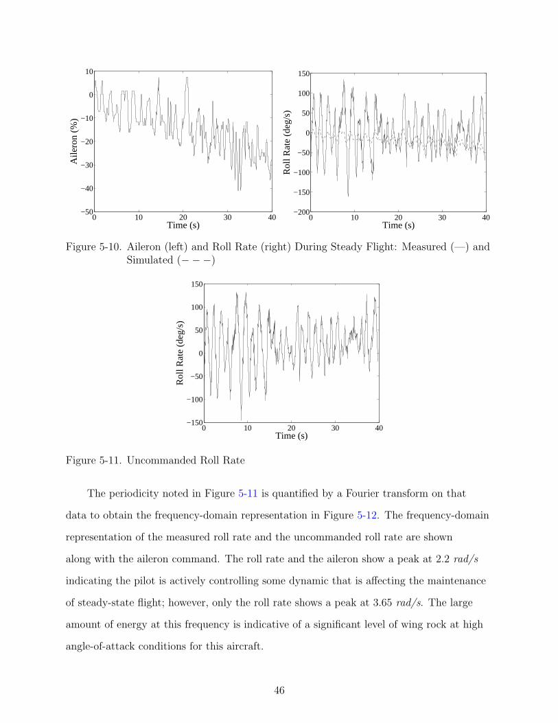
The uncommanded portion of the response, as determined by subtracting the
simulated response to the aileron from the measured response, is shown in Figure 5-11.
This portion is quite large in magnitude and actually appears quite periodic.
45
0 10 20 30 40−50
−40
−30
−20
−10
0
10
Time (s)
Aile
ron
(%)
0 10 20 30 40−200
−150
−100
−50
0
50
100
150
Time (s)
Rol
l Rat
e (d
eg/s
)
Figure 5-10. Aileron (left) and Roll Rate (right) During Steady Flight: Measured (—) andSimulated (−−−)
0 10 20 30 40−150
−100
−50
0
50
100
150
Time (s)
Rol
l Rat
e (d
eg/s
)
Figure 5-11. Uncommanded Roll Rate
The periodicity noted in Figure 5-11 is quantified by a Fourier transform on that
data to obtain the frequency-domain representation in Figure 5-12. The frequency-domain
representation of the measured roll rate and the uncommanded roll rate are shown
along with the aileron command. The roll rate and the aileron show a peak at 2.2 rad/s
indicating the pilot is actively controlling some dynamic that is affecting the maintenance
of steady-state flight; however, only the roll rate shows a peak at 3.65 rad/s. The large
amount of energy at this frequency is indicative of a significant level of wing rock at high
angle-of-attack conditions for this aircraft.
46

10−1
100
101
102
10−2
100
102
104
Frequency (rad/s)
Mag
nitu
de
Figure 5-12. FFT of Measured Roll Rate (...), Uncommanded Roll Rate (—), and AileronInput (−−−)
5.3.3 Directional
The steady-state characteristics of the directional dynamics is investigated using the
data in Figure 5-13. This data consists of small rudder commands to maintain the flight
condition and the associated yaw rates which were measured and simulated from the
model in Equation 5–5.
0 10 20 30 40 50−30
−20
−10
0
10
20
30
40
Time (s)
Rud
der
(%)
0 10 20 30 40 50−60
−40
−20
0
20
40
60
80
Time (s)
Yaw
Rat
e (d
eg/s
)
Figure 5-13. Rudder (left) and Yaw Rate (right) During Steady Flight: Measured (—) andSimulated (−−−)
47

The amount of yaw rate which can not be predicted by the model is given in
Figure 5-14. The yaw rate also has some clear periodicity and a substantial magnitude
indicating some element of steady-state flight is not captured by the model generated from
doublets.
0 10 20 30 40 50−40
−20
0
20
40
60
80
Time (s)
Yaw
Rat
e (d
eg/s
)
Figure 5-14. Uncommanded Yaw Rate
The frequency-domain representation of the yaw rate, both measured and uncommanded,
along with rudder commands indicates the periodicity. This data, as shown in Figure 5-15,
has a noticeable mode near 2.2 rad/s. Both the rudder and the yaw rate contain this
mode, as did the aileron and the roll rate, which may mean it correlates to a roll-yaw
coupled mode that the pilot is attempting to damp out and maintain condition.
Figure 5-15 indicates frequency regions where the uncommanded yaw rate is of
larger correlation than the measured yaw rate, particularly between approximately 2.5
and 5 rad/s and 6 and 10 rad/s. This seems improper, as the uncommanded yaw rate is
extracted from the measured yaw rate and should therefore be a subset of the measured
yaw rate. However, phase shifts between the model-predicted yaw rate and the measured
yaw rate can result in uncommanded yaw rates estimated at higher values than the
measured yaw rate.
48

10−1
100
101
102
10−2
100
102
104
Frequency (rad/s)
Mag
nitu
de
Figure 5-15. FFT of Measured Yaw Rate (...), Uncommanded Yaw Rate (—), and RudderInput (−−−)
49

CHAPTER 6VERTICAL TAIL RELATIONSHIP TO WING ROCK
6.1 Upright Tail
A series of flight tests are performed with the airplane in an upright orientation with
different vertical tails. Roll rates were examined as the primary indicator of wing rock
characteristics.
The roll rate measured during these tests is shown in Figure 6-1 along with the
associated aileron deflections. The aileron deflection is dramatically smaller than the
roll rate and thus difficult to distinguish. Clearly the roll rate shows some amount of
periodicity among all the tails; consequently, wing rock appears for any size of these tails.
Also, the magnitude of the roll rate shows variation during the response; however, this
magnitude is actually somewhat consistent despite variations in the tail size.
A frequency-domain representation of the roll rates and aileron deflections from
Figure 6-1 is computed and shown in Figure 6-2 using a Fourier transform. The roll rate
shows a consistent amount of energy around 4 rad/s which correlates with the consistent
magnitude observed in the time-domain responses. Very little energy is introduced by
the aileron around 4 rad/s, indicating that the energy observed in figure 6-2 represents
uncommanded wing rock. Also, this peak in energy is actually somewhat broad for every
tail and ranges from approximately 2 rad/s to 6 rad/s indicating the wing rock is a
broad-band phenomenon.
A time-frequency representation is computed for the roll rate to investigate the
temporal nature of any instantaneous frequencies in the wing rock. These representations
are shown in Figure 6-3 as computed by wavelet transforms using a Morlet wavelet.
The wing rock is evident by the high correlations shown around 4 rad/s; however,
this representation is notably different than the frequency-domain characterization in
Figure 6-2. The wing rock is shown to actually have a narrow band of energy when
50

020
4060
8010
0−
150
−10
0
−5005010
0
150
Tim
e (s
)
Magnitude
020
4060
8010
0−
150
−10
0
−5005010
0
150
Tim
e (s
)
Magnitude
020
4060
−15
0
−10
0
−5005010
0
150
Tim
e (s
)
Magnitude
020
4060
8010
0−
150
−10
0
−5005010
0
150
Tim
e (s
)
Magnitude
050
100
150
−15
0
−10
0
−5005010
0
150
Tim
e (s
)
Magnitude
Fig
ure
6-1.
Tim
eR
espon
ses
inU
pri
ght
Con
figu
rati
onfo
rA
)Sm
alle
rTai
l,B
)Sm
allTai
l,C
)N
orm
alTai
l,D
)B
igTai
l,E
)B
igge
rTai
l:R
ollR
ate
(—)
inde
g/s
and
Ailer
onD
eflec
tion
(...)
in%
51

10−1
100
101
102
100
102
104
106
Roll Rate FFTs
Frequency (rad/s)
Mag
nitu
de
10−1
100
101
102
100
102
104
106
Roll/Aileron FFt
Frequency (rad/s)
Mag
nitu
de
Figure 6-2. FFT in Upright Configuration of Roll Rate (left) and Aileron Deflection(right): Smaller Tail (– –), Small Tail (–.–.), Normal Tail (—), Big Tail (...),Bigger Tail (–x–)
localized in time using Figure 6-3. The broad-band nature observed in Figure 6-2 results
from the variations observed in Figure 6-3 in the central frequency of that narrow band.
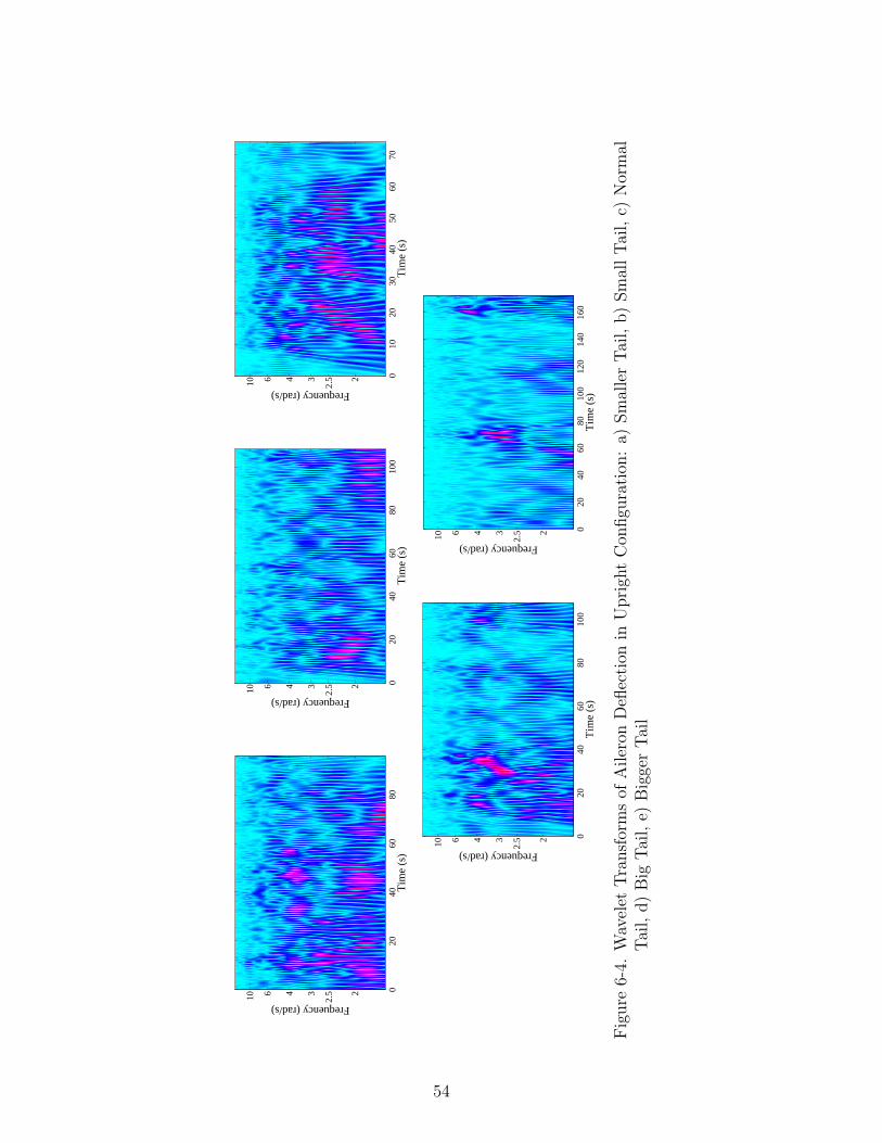
The wavelet transforms of the aileron deflection, as shown in Figure 6-4, do not
show significant correlation with the wing rock. In each case, the aileron deflections are
predominately at lower frequencies.
6.2 Inverted Tail
The airplane is flown in an inverted configuration for each of the different sizes of
vertical tail. The roll rate measured during these tests is shown in Figure 6-5 along with
the associated aileron deflections. The roll rates are approximately an order of magnitude
greater than the aileron deflections although both appear to have periodicity. In each case,
this magnitude and periodicity are relatively consistent despite variations to the tail.
The frequency-domain representations, shown in Figure 6-6, agree with the time-domain
analysis of Figure 6-5. The energy of the roll rate is about an order of magnitude greater
than the aileron for each tail. Also, the roll rate shows a minor broad-band peak near
4 rad/s although the energy is not excessive.
A wavelet transform is applied to the time-domain data to generate the representation,
shown in Figure 6-7, in the time-frequency domain. These plots show some correlation
52

Tim
e (s
)
Frequency (rad/s)
020
4060
80
23410 6
2.5
Tim
e (s
)
Frequency (rad/s)
020
4060
8010
0
2
2.534610
Tim
e (s
)
Frequency (rad/s)
010
2030
4050
6070
2
2.534610
Tim
e (s
)
Frequency (rad/s)
020
4060
8010
0
2
2.534610
Tim
e (s
)Frequency (rad/s)
020
4060
8010
012
014
016
0
2
2.534610
Fig
ure
6-3.
Wav
elet
Tra
nsf
orm
sof
Rol
lR
ate
inU
pri
ght
Con
figu
rati
on:
A)
Sm
alle
rTai
l,B
)Sm
allTai
l,C
)N
orm
alTai
l,D
)B
igTai
l,E
)B
igge
rTai
l
53
Tim
e (s
)
Frequency (rad/s)
020
4060
80
2
2.534610
Tim
e (s
)
Frequency (rad/s)
020
4060
8010
0
2
2.534610
Tim
e (s
)
Frequency (rad/s)
010
2030
4050
6070
2
2.534610
Tim
e (s
)
Frequency (rad/s)
020
4060
8010
0
2
2.534610
Tim
e (s
)Frequency (rad/s)
020
4060
8010
012
014
016
0
2
2.534610
Fig
ure
6-4.
Wav
elet
Tra
nsf
orm
sof
Ailer
onD
eflec
tion
inU
pri
ght
Con
figu
rati
on:
a)Sm
alle
rTai
l,b)
Sm
allTai
l,c)
Nor
mal
Tai
l,d)
Big
Tai
l,e)
Big
ger
Tai
l
54

010
2030
4050
60−
150
−10
0
−5005010
0
150
Tim
e (s
)
Magnitude
010
2030
4050
60−
150
−10
0
−5005010
0
150
Tim
e (s
)
Magnitude
010
2030
4050
60−
150
−10
0
−5005010
0
150
Tim
e (s
)
Magnitude
020
4060
80−
150
−10
0
−5005010
0
150
Tim
e (s
)
Magnitude
020
4060
−15
0
−10
0
−5005010
0
150
Tim
e (s
)
Magnitude
Fig
ure
6-5.
Tim
eR
espon
ses
inIn
vert
edC
onfigu
rati
onfo
rA
)Sm
alle
rTai
l,B
)Sm
allTai
l,C
)N
orm
alTai
l,D
)B
igTai
l,E
)B
igge
rTai
l:R
ollR
ate
(—)
and
Ailer
onD
eflec
tion
(...)
55

10−1
100
101
102
100
102
104
106
Roll Rate FFTs
Frequency (rad/s)
Mag
nitu
de
10−1
100
101
102
100
102
104
106
Roll/Aileron FFt
Frequency (rad/s)
Mag
nitu
de
Figure 6-6. FFT in Inverted Configuration of Roll Rate (left) and Aileron Deflection(right): Smaller Tail (– –), Small Tail (–.–.), Normal Tail (—), Big Tail (...),Bigger Tail (–x–)
around 4 rad/s; however, the magnitude of correlation is not excessively high in comparison
to the lower frequencies. This lack of excessive correlation agrees with the Fourier
transforms in Figure 6-6 and is evident for each tail.
A similar time-frequency representation of the aileron data, as computed through
wavelet transform and shown in Figure 6-8, indicates a strong correlation to the roll rates
that are shown in Figure 6-7. In particular, most of the peaks in correlation for roll rate
are matched by a peak in aileron at the same time and frequency. Examples of such
input/output matching can be seen with the smaller tail at approximately 2.5 to 3 rad/s
between 50 and 60 s and with the bigger tail at approximately 3 rad/s between 10 and
20 s and at approximately 3 to 4 rad/s between 45 and 60 s.
6.3 Parameterization
The time-domain plots of roll rate in upright and inverted high angle-of-attack flight,
shown in Figures 6-1 and 6-5 respectively, are analyzed. Peak averages and frequencies are
extracted for each vertical tail size and shown in Figure 6-9.
The time-domain analysis in Figure 6-9 indicates that wing rock frequency and
magnitude does not depend upon the size of the vertical tail. However, the wing rock
magnitude does change based on the vertical tail configuration: the average wing rock
56

Tim
e (s
)
Frequency (rad/s)
010
2030
4050
2
2.534610
Tim
e (s
)
Frequency (rad/s)
010
2030
4050
60
2
2.534610
Tim
e (s
)
Frequency (rad/s)
010
2030
4050
60
2
2.534610
Tim
e (s
)
Frequency (rad/s)
010
2030
4050
6070
2
2.534610
Tim
e (s
)Frequency (rad/s)
010
2030
4050
60
2
2.534610
Fig
ure
6-7.
Wav
elet
Tra
nsf
orm
sof
Rol
lR
ate
inIn
vert
edC
onfigu
rati
on:
A)
Sm
alle
rTai
l,B
)Sm
allTai
l,C
)N
orm
alTai
l,D
)B
igTai
l,E
)B
igge
rTai
l
57

Tim
e (s
)
Frequency (rad/s)
010
2030
4050
2
2.534610
Tim
e (s
)
Frequency (rad/s)
010
2030
4050
60
2
2.534610
Tim
e (s
)
Frequency (rad/s)
010
2030
4050
60
2
2.534610
Tim
e (s
)
Frequency (rad/s)
010
2030
4050
6070
2
2.534610
Tim
e (s
)Frequency (rad/s)
010
2030
4050
60
2
2.534610
Fig
ure
6-8.
Wav
elet
Tra
nsf
orm
sof
Ailer
onD
eflec
tion
inIn
vert
edC
onfigu
rati
on:
A)
Sm
alle
rTai
l,B
)Sm
allTai
l,C
)N
orm
alTai
l,D
)B
igTai
l,E
)B
igge
rTai
l
58

Figure 6-9. Mean Roll Rate Peak Magnitudes (—) and Peak-to-Peak Frequencies (...)
peak magnitude in the inverted flight condition is approximately half of that in the
upright flight condition across all tail sizes. The average wing rock frequency is nearly
constant at approximately 4 rad/s for all tail sizes in both upright and inverted high
angle-of-attack flight, which agrees with the peaks seen in the Fourier transforms in
Figures 6-2 and 6-6.
The difference in magnitude of uncommanded wing rock between upright and inverted
flight is likely more pronounced than Figure 6-9 indicates. Figures 6-3 and 6-4 show little
correlation between aileron input and roll rate frequencies in the upright configuration.
Figures 6-7 and 6-8 indicate, however, that a strong correlation exists between roll
rate and aileron input frequencies at essentially all times when roll rate oscillations are
observed in the inverted configuration. This indicates that uncommanded wing rock is
virtually nonexistent when in the inverted configuration.
The upper and lower bounds of wing rock frequency are extracted from Figures 6-2
and 6-3 and are shown in Figure 6-10. Only the upright configuration is analyzed for such
bounds because only uncommanded wing rock is of interest. The upper and lower bounds
as determined by both the FFTs and wavelets are fairly consistent for all upright tail
59

sizes. These bounds indicate that wing rock exists across a spectrum of frequencies, with
bandwidths of approximately 2 rad/s for all tail sizes.
Figure 6-10. Upper and Lower Bounds of Wing Rock Frequency from FFTs (—) andWavelets (...)
The time-frequency representations shown in Figure 6-3 actually indicate that
the wing rock oscillation is much narrower in bandwidth when localized in time than
Figure 6-10 indicates. The average bandwidth of the wing rock oscillations at all times
for each tail are extracted from the wavelet plots and are shown in Figure 6-11 along with
the broad bands extracted from Figure 6-10. The bandwidth at most times is notably
smaller in Figure 6-11 than in Figure 6-10. This indicates that wing rock is actually a
fairly narrow-band phenomenon, but variations in frequency over time within a broader
band lead to the appearance of a broad-band phenomenon with many classical analysis
techniques such as the FFT.
60

Figure 6-11. Mean Wing Rock Bandwidths: FFT (—), Wavelet Broad Limits (...), andWavelet Narrow Limits (– – –)
61

CHAPTER 7SUMMARY
7.1 Recommendations
High angle-of-attack flight can expand the flight envelope of a small UAV if it has
sufficient thrust-to-weight ratio and control surface size and deflection. The expanded
regions of the flight envelope, including lower airspeed limits and smaller recovery area
requirements, can enhance mission capability if maneuvering control can be achieved. As
such, modeling the flight dynamics is required to analyze the appropriateness of various
control schemes in this unconventional realm of flight.
The models identified from the flight data are somewhat limited in usefulness.
The models may be applicable with slight modifications to other aircraft with similar
configurations and sizing, but their usefulness beyond such a narrow range of aircraft
is unknown. The least-squares models display the general simplicity and complexity of
modeling the various axes of the aircraft dynamics. However, they do not accurately
predict substantial uncommanded motion that appears to be present about all three axes.
Additionally, the lack of angle-of-attack and angle-of-sideslip measurements or
estimates introduces uncertainty in modeling. Work is currently underway to obtain
inertial-based estimates of both such angles from the current avionics suite. The inclusion
of such parameters could greatly improve the accuracy of the models and permit higher
fidelity modeling approaches.
Angle-of-attack and sideslip estimates could also improve the ability to analyze wing
rock behavior in conjunction with time-frequency analysis techniques. Of particular
interest in future studies is the relationship between the wing rock frequency and
the angle-of-attack. A correlation between the variations in wing rock frequency and
fluctuations in angle-of-attack would be an extremely useful result. A lack of any
correlation between such parameters would also be notable finding.
62

The dependency of wing rock on vertical tail configuration is a useful result.
Further study of wing rock characteristics could analyze dependencies on other airframe
geometries, such as V-tail and twin-tail configurations, combined upper and lower vertical
tails, wingtip endplates, and flap/spoiler configurations.
An additional branch of future studies on this topic could include analyzing high
angle-of-sideslip flight. The high angle-of-sideslip flight realm is utilized very little in
practical applications; however, it could potentially increase maneuverability for operations
within urban environments or aid in sensor pointing for various surveillance and sensing
missions.
7.2 Conclusion
The flight dynamics at high angle-of-attack conditions are challenging to model.
An extensive set of data from a remote-controlled Mini Showtime aircraft is analyzed
in response to both commanded doublets and steady-state flight. The responses to
doublets demonstrate that the lateral dynamics are relatively straightforward to model
with a dominant roll convergence mode, while the longitudinal dynamics and directional
dynamics need nonlinearities and numerous states along with lags to properly represent
the flight characteristics. The responses at steady-state flight are particularly interesting
in that the roll rate indicates a significant contribution from wing rock while both the
roll rate and yaw rate have a contribution from a mode that the pilot is attempting to
damp. As such, a partial analysis of the behavior at high angle-of-attack conditions is
generated that demonstrates phenomena and characteristics that are not as evident at low
angle-of-attack conditions.
Uncommanded wing rock at high angle-of-attack flight is a complex phenomenon.
An extensive set of high angle-of-attack flight data from the Mini ShowTime aircraft
with multiple vertical tail sizes and configurations is analyzed. The aircraft has very few
asymmetries, except for the vertical tail, which allows upright and inverted flight to be
compared. Time-frequency analysis indicates that when the vertical tail is in the upright
63

position, pronounced uncommanded wing rock is present at approximately 4 rad/s for all
sizes of vertical tail. Uncommanded wing rock was virtually eliminated when a vertical tail
of any size was in the inverted configuration. These findings indicate that for this aircraft
uncommanded wing rock is greatly influenced by the presence or absence of upright and
inverted vertical tails, but not necessarily the size of such vertical tails.
64

REFERENCES
[1] Wright, K., and Lind, R., “Investigating Sensor Emplacement on Vertical Surfacesfor a Biologically-Inspired Morphing Design from Bats,” AIAA Paper 2007-6488,Aug. 2007.
[2] Grant, D., Abdulrahim, M., and Lind, R., “Flight Dynamics of a Morphing AircraftUtilizing Multiple-Joint Wing Sweep,” AIAA Paper 2006-6505, Aug. 2006.
[3] Regenie, V., Gatlin, D., Kempel, R., and Matheny, N., “The F-18 High AlphaResearch Vehicle: A High-Angle-of-Attack Testbed Aircraft,” NASA TM 104253,1992.
[4] Iliff, K., and Wang, K., “Flight Determined Subsonic Longitudinal Stability andControl Derivatives of the F-18 High Angle of Attack Research Vehicle (HARV)With Thrust Vectoring,” NASA TP 97-206539, 1997.
[5] Bauer, J., Clarke, R., and Burken, J., “Flight Test of the X-29A at High Angle ofAttack: Flight Dynamics and Controls,” NASA TP 3537, 1995.
[6] NASA Dryden F-18 High Alpha Research Vehicle (HARV) Photo Collection.July 26, 2001. National Aeronautics and Space Administration. Feb. 23, 2009<http://www.dfrc.nasa.gov/gallery/Photo/F-18HARV/>.
[7] NASA Dryden X-29 Photo Collection. Feb. 3, 2000. National Aeronautics and SpaceAdministration. Feb. 23, 2009 <http://www.dfrc.nasa.gov/gallery/Photo/X-29/>.
[8] AeroVironment Unmanned Aircraft Systems, <http://avinc.com/UAS.asp>.
[9] Quigley, M., Barber, B., Griffiths, S., and Goodrich, M., “Towards Real-WorldSearching with Fixed-Wing Mini-UAVs,” IEEE/RSJ International Conference onIntelligent Robots and Systems, Aug. 2005.
[10] AeroVironment, Inc.: Media Gallery. 2009. AeroVironment, Inc. Feb. 23, 2009<http://www.avinc.com/media gallery2.asp?id=224>.
[11] Frank, A., McGrew, J., Valenti, M., Levine, D., and How, J., “Hover, Transition,and Level Flight Control Design for a Single-Propeller Indoor Airplane,”AIAA Paper 2007-6318, Aug. 2007.
[12] Johnson, E., Turbe, M., Wu, A., Kannan, S., and Neidhoefer, J., “Flight TestResults of Autonomous Fixed-Wing UAV Transitions to and from StationaryHover,” AIAA Paper 2006-6775, Aug. 2006.
[13] Gree, W., and Oh, P., “Autonomous Hovering of a Fixed-Wing Micro Air Vehicle,”IEEE International Conference on Robotics and Automation, May 2006.
[14] Hwang, C., and Pi, W. S., “Some Observations on the Mechanism of Aircraft WingRock,” Journal of Aircraft, Vol. 16, No. 6, pp. 366-373, 1979.
65

[15] Liebst, B., Nolan, R., “Method for the Prediction of the Onset of Wing Rock,”Journal of Aircraft, Vol. 31, No. 6, pp. 1419-1421, 1994.
[16] Regenie, V., Gatlin, D., Kempel, R., and Matheny, N., “The F-18 High AlphaResearch Vehicle: A High-Angle-of-Attack Testbed Aircraft,” NASA TM 104253,1992.
[17] Ramnath, R. V., and Go, T. H., “An Analytical Approach to the Aircraft WingRock Dynamics,” AIAA Paper 2001-4426, 2001.
[18] Go, T. H., and Ramnath, R. V., “An Analysis of the Two Degree-of-Freedom WingRock on Advanced Aircraft,” Journal of Guidance, Control, and Dynamics, Vol. 25,No. 2, pp. 324-333, 2002.
[19] Schmidt, L. V., “Wing Rock Due to Aerodynamic Hysteresis,” Journal of Aircraft,Vol. 16, No. 3, pp. 129-133, 1979.
[20] Lie, F. A. P., and Go, T. H., “Analysis of Single Degree-of-Freedom Wing Rock dueto Aerodynamic Hysteresis,” AIAA Paper 2007-6489, 2007.
[21] Abramov, N., Goman, M., Demenkov, M., and Khabrov, A., “Lateral-DirectionalAircraft Dynamics at High Incidence Flight with Account of Unsteady AerodynamicEffects,” AIAA Paper 2005-6331, 2005.
[22] Bauer, J., Clarke, R., and Burken, J., “Flight Test of the X-29A at HighAngle-of-Attack: Flight Dynamics and Controls,” NASA TP 3537, 1995.
[23] Liebst, B. S., and DeWitt, B. R., “Wing Rock Suppression in the F-15 Aircraft,”AIAA Paper 1997-3719, 1997.
[24] Iliff, K. W., and Wang, K. C., “X-29A Lateral-Directional Stability and ControlDerivatives Extracted from High-Angle-of-Attack Flight Data,” NASA TP 3664,1996.
[25] Davison, M. T., “An Examination of Wing Rock for the F-15,” Master’s Thesis, AirForce Inst. of Technology, AFIT/GAE/ENY/92M-01, Feb. 1992.
[26] Brandon, J. M., and Nguyen, L. T., “Experimental Study of Effects of ForebodyGeometry on High Angle-of-Attack Stability,” Journal of Aircraft, Vol. 25, No. 7,pp. 591-597, 1988.
[27] Meyer, R. R., “Overview of the NASA Dryden Flight Research Facility AeronauticalFlight Projects,” NASA TM 104254, 1992.
[28] Ericsson, L. E., “Various Sources of Wing Rock,” Journal of Aircraft, Vol. 27, No. 6,pp. 488-494, 1990.
66

[29] Walton, J., and Katz, J., “Application of Leading-Edge Vortex Manipulations toReduce Wing Rock Amplitudes,” Journal of Aircraft, Vol. 30, No. 4, pp. 555-557,1993.
[30] Ericcson, L. E., “Sources of High Alpha Vortex Asymmetry at Zero Sideslip,”Journal of Aircraft, Vol. 29, No. 6, pp. 1086-1090, 1992.
[31] Ericsson, L. E., “Wing Rock Generated by Forebody Vortices,” Journal of Aircraft,Vol. 26, No. 2, pp. 110-116, 1989.
[32] Ericsson, L. E., “Further Analysis of Wing Rock Generated by Forebody Vortices,”Journal of Aircraft, Vol. 26, No. 22, pp. 1098-1104, 1989.
[33] L. E. Ericsson, “Effect of Deep-Stall dynamics on Forebody-Induced Wing Rock,”AIAA Paper 1996-3404, 1996.
[34] Alcorn, C. W., Croom, M. A., Francis, M. S., and Ross, H., “The X-31 Aircraft:Advances in Aircraft Agility and Performance,” Progress in Aerospace Sciences,Vol. 32, pp. 377-413, 1996.
[35] Gilbert, W. P., Nguyen, L. T., and Gera, J., “Control Research in the NASAHigh-Alpha Technology Program,” AGARD Fluid Dynamics Panel Symposium onAerodynamics of Combat Aircraft Control and Ground Effects, 1989.
[36] Mini ShowTime 4D ARF by E-flite (EFL2500), Horizon Hobby, Inc.,<http://www.horizonhobby.com>, Champaign, IL, 2006-2009.
[37] Smith, H. C., The Illustrated Guide to Aerodynamics, TAB Books, Blue RidgeSummit, PA, pp. 228-229, 1992.
[38] nIMU Datasheet Version 2.7, MEMSense, LLC, <http://www.memsense.com>,Rapid City, SD, 2007.
[39] Instruction Manual for the USB Flight Data Recorder Version 3.7, Eagle TreeSystems, LLC, <http://www.eagletreesystems.com>, Bellevue, WA, 2003-2005.
[40] Perry, J., Mohamed, A., Johnson, B., and Lind, R., “Estimating Angle of Attack andSideslip Under High Dynamics on Small UAVs,” Proceedings of the 21st Interna-tional Technical Meeting of the Satellite Division of the Institute of Navigation IONGNSS 2008, pp. 1165-1173, 2008.
[41] Misiti, M., Misiti, Y., Oppenheim, G., and Poggi, J., Wavelet Toolbox User’s Guide,Version 2, The MathWorks, Inc., Natick, MA, Chap. 1,6, 2000.
[42] Strang, G., Nguyen, T., Wavelets and Filter Banks, Wellesley-Cambridge Press,Wellesley, MA, Chap. 1, 1996.
[43] Klein, V., and Morelli, E. A., Aircraft System Identification Theory and Practice,AIAA Education Series, AIAA, Reston, VA, Chap. 5, 2006.
67

[44] Yechout, T., Introduction to Aircraft Flight Mechanics, AIAA Education Series,AIAA, Reston, VA, pp. 176-177, 2003.
68

BIOGRAPHICAL SKETCH
Baron Johnson’s aviation pursuits began with his first aerobatic rides a few days
prior to being born in Memphis, TN in 1983. After moving to Ocala, FL, Baron soloed an
L23 Super Blanik sailplane at the age of 14, and then soloed a Piper J-3 Cub on his 16th
birthday. Baron then pursued his private pilot license, which he received at the age of 17,
and his commercial pilot license, which he received at the age of 18, along with instrument
and multi-engine ratings. Baron has accumulated over 600 hours of flight experience,
including very unique opportunities such as flying in part of a 60-ship formation of and
serving as in-flight safety observer in the EAA AirVenture airshow.
After graduating from Belleview High School in 2002, Baron attended the University
of Florida in Gainesville, FL. He graduated cum laude with a Bachelor of Science in
aerospace engineering in 2007, and received a Master of Science in aerospace engineering
in 2009. While studying, Baron has had opportunities to work on many exciting UAV and
MAV programs while employed by the Florida Cooperative Fish & Wildlife Research Unit,
Micro Air Vehicle Lab, and Flight Control Lab. While member and pilot for the UF Micro
Air Vehicle Team, the team captured 4 consecutive victories at the International Micro Air
Vehicle Competition.
Baron has also been an active RC aviator during his years. His primary passions
in RC are IMAC Scale Aerobatics and F3C Helicopter Aerobatics. Baron has had the
opportunity to fly many RC demonstrations and competitions, and has won 4 national
championship titles along with other high finishes at international competitions.
Baron also authored a children’s book titled History Takes A Wild Ride, for which
he was awarded the key to the city of Memphis and appeared on NBC’s The Today Show.
Baron has had some incredible experiences and opportunities in his life for which he is
incredibly grateful.
69