herbert yoo and paul green - university of michigandriving/publications/umtri-99-14.pdffinal, 9/94 -...

Driver Behavior While FollowingCars, Trucks, and Buses

Herbert Yoo and Paul Green

May, 1999Technical Report UMTRI-99-14

umtriHUMAN FACTORS

Technical Report Documentation Page

1. Report No.

UMTRI-99-142. Government Accession No. 3. Recipient’s Catalog No.

4. Title and Subtitle

Driver Behavior While Following5. Report Date

May, 1999Cars, Trucks, and Buses 6. Performing Organization Code

account 0321217. Author(s)

Herbert Yoo and Paul Green8. Performing Organization Report No.

UMTRI-99-149. Performing Organization Name and Address

The University of Michigan10. Work Unit no. (TRAIS)

Transportation Research Institute (UMTRI)2901 Baxter Rd, Ann Arbor, Michigan 48109-2150

11. Contract or Grant No.

12. Sponsoring Agency Name and Address

Great Lakes Center for Truck and Transit Research13. Type of Report and Period Covered

final, 9/94 - 5/99University of Michigan Transportation Research InstituteAnn Arbor, Michigan 48109-2150 USA

14. Sponsoring Agency Code

15. Supplementary Notes

16. Abstract

A total of 16 drivers (8 ages 16-30, 8 ages 65 or older) drove a driving simulator atapproximately 45 mi/hr while following either a car, pickup truck, school bus, or tractortrailer. They drove on a winding two-lane road as they normally would, but wereinstructed not to pass the lead vehicle. The variance of the lead vehicles was eitherlow (4.2 mi/hr) or high (for the car and pickup truck only, 7.1 mi/hr). They alsoidentified signs when they appeared.

In general, older drivers followed at a greater distance than younger drivers (469 vs.282 ft) and some older drivers followed so the lead vehicle would be out of sight(600 ft). These following distances, corresponding to headway times of 4.3 and 7.1 s,are much greater than are typically reported from on-the-road studies.

Although subjects followed cars about 10 percent closer than other vehicles, therewere no other effects of vehicle type or its speed variability (within the range explored)on following distance. Further, both mean lateral position and the standard deviationof lateral position were unaffected by lead vehicle type or their speed variance,though there were significant individual differences. The lack of influence of vehiclecharacteristics may result from the absence of following traffic (and a rear view mirrorto see such) in this simulation, so the pressure to keep up with traffic was missing.This suggests that following studies may require simulations to include a rear visualchannel.17. Key Words

ITS, human factors, ergonomics,driving, collision avoidance, trafficdriving science, normal driving

18. Distribution Statement

No restrictions. This document isavailable to the public through theNational Technical Information Service,Springfield, Virginia 22161

19. Security Classify. (of this report)

none20. Security Classify. (of this page)

none21. No. of pages

**22. Price

Form DOT F 1700 7 (8-72) Reproduction of completed page authorized

Driver Behavior While Following Cars, Trucks, and Buses

ISSUES1

METHOD (simulator)2

RESULTS3

UMTRI Technical Report 99-14Herbert Yoo and Paul Green

iii

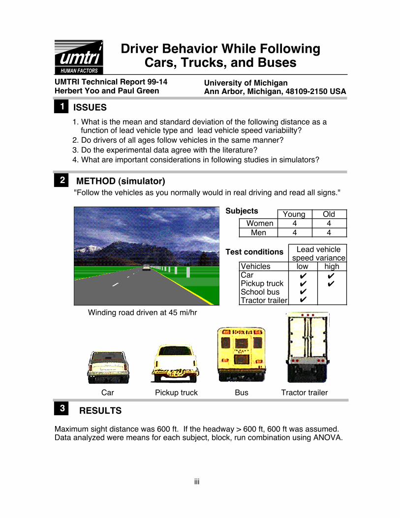
Subjects Young OldWomen 4 4

Men 4 4

1. What is the mean and standard deviation of the following distance as a function of lead vehicle type and lead vehicle speed variabiilty?

2. Do drivers of all ages follow vehicles in the same manner? 3. Do the experimental data agree with the literature?4. What are important considerations in following studies in simulators?

University of MichiganAnn Arbor, Michigan, 48109-2150 USA

"Follow the vehicles as you normally would in real driving and read all signs."

Maximum sight distance was 600 ft. If the headway > 600 ft, 600 ft was assumed.Data analyzed were means for each subject, block, run combination using ANOVA.

Test conditions

Car Pickup truck Bus Tractor trailer

Winding road driven at 45 mi/hr

Lead vehicle speed varianceVehicles low highCar Pickup truck School busTractor trailer

✔✔✔✔

✔✔

CONCLUSIONS4

0250500750

10001250150017502000

0 100 200 300 400 500 600

14448

Old men

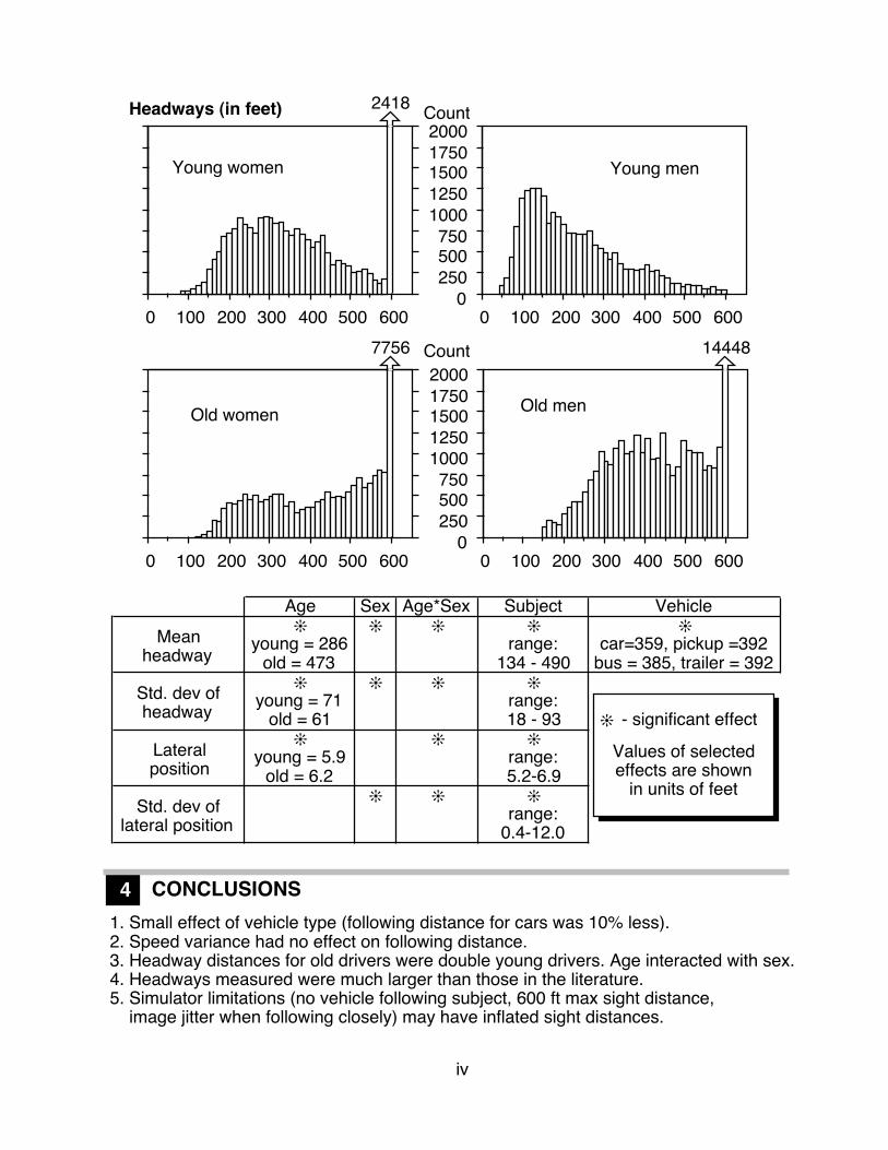
1. Small effect of vehicle type (following distance for cars was 10% less).2. Speed variance had no effect on following distance.3. Headway distances for old drivers were double young drivers. Age interacted with sex.4. Headways measured were much larger than those in the literature.5. Simulator limitations (no vehicle following subject, 600 ft max sight distance, image jitter when following closely) may have inflated sight distances.

Headways (in feet)

iv

0 100 200 300 400 500 6000

250500750

10001250150017502000

Young men

Count

Age Sex Age*Sex Subject Vehicle

Mean❊ ❊ ❊ ❊ ❊

headwayyoung = 286 range: car=359, pickup =392

old = 473 134 - 490 bus = 385, trailer = 392

Std. dev of❊ ❊ ❊ ❊

headwayyoung = 71 range:

old = 61 18 - 93❊ ❊ ❊

Lateral position

young = 5.9 range:old = 6.2 5.2-6.9

Std. dev of❊ ❊ ❊

lateral positionrange:

0.4-12.0

❊ - significant effect

Values of selected effects are shown

in units of feet

0 100 200 300 400 500 600

2418

Young women

0 100 200 300 400 500 600

7756

Old women

Count

v

PREFACE

The purpose of this project was to examine driver following behavior in a simulator,and as part of that process, upgrade the UMTRI driving simulator. Independent of theprimary research questions, there were two major technical challenges: (1) getting thelead vehicle to maneuver in a realistic manner, and (2) scanning and editing the leadvehicle images so that they appeared realistic. The authors would like to thank AlanOlson of UMTRI for his efforts to design and implement the autopilot routines forcontrolling lead vehicles. Edgar Manalo (formerly of UMTRI) played a major role increating the graphics files for lead vehicles and constructing the experiment scenarios.

vi

TABLE OF CONTENTS

INTRODUCTION ........................................................................................ 1Evidence from the Literature on Crash Statistics....................................................... 1Studies of How People Actually Follow Traffic........................................................... 1Issues................................................................................................................................. 4

TEST PLAN ............................................................................................... 5Overview............................................................................................................................ 5Test Participants............................................................................................................... 5Test Materials and Equipment....................................................................................... 6Test Activities and Sequence......................................................................................10

RESULTS ................................................................................................ 1 3Data Analysis Methods and ANOVA Approach .......................................................13What Affects Following Distance? ..............................................................................14What Affects Following Distance Variability? ...........................................................17What Affects Mean Lateral Position? .........................................................................19What Affects the Standard Deviation of Lateral Position? .....................................19Subjective Evaluation of the Simulation ...................................................................20

CONCLUSIONS....................................................................................... 2 3What Affects Following Distance and Its Variability? ..............................................23What Affects the Lateral Position and Lateral Variability of a FollowingVehicle?...........................................................................................................................23What Are Important Considerations in Simulator-Based FollowingStudies? ..........................................................................................................................23Closing Comment..........................................................................................................24

REFERENCES ......................................................................................... 2 5

APPENDIX A - DESCRIPTION OF ROADS............................................... 2 9

APPENDIX B - CONSENT FORM ............................................................. 3 1

APPENDIX C - BIOGRAPHICAL FORM .................................................... 3 3

APPENDIX D - EXPERIMENT INSTRUCTIONS........................................ 3 5

APPENDIX E - LEAD VEHICLE DYNAMICS ............................................ 3 9

APPENDIX F - EVALUATION FORM......................................................... 4 7

APPENDIX G - ANOVA TABLES .............................................................. 5 1

1

INTRODUCTION

Under the guise of ITS (Intelligent Transportation Systems) there is significant interestin implementing new systems to make driving safer, more efficient, and moreenjoyable. Products are being developed to provide navigation assistance, warndrivers of various types of collisions, provide information on various motoring-relatedservices, provide for automatic and semiautomatic lane keeping and speed control,and so forth. Some of these products could radically change the way people drive. Ifthat is the case, then there is a need for a fundamental understanding of how peopledrive, that is, to develop a science of driving. First, to determine where improvementsare possible, there is a need to know what drivers do now. Second, when prototypesof new systems are available, baseline data are needed to assess if any change hasoccurred. Finally, there is a more general need to develop models of how peopledrive, allowing design alternatives to be assessed using inexpensive computationmethods rather than expensive experimental evaluations (van Winsum, 1991). As anexample, such data such data has proven to be useful in predicting the effectivenessof alternative collision warning algorithms (Farber, 1995). To collect data on driving,cost-effective tools will be needed including instrumented vehicles, road monitoringsystems, and driving simulators.

Evidence from the Literature on Crash Statistics

One of the more commonly referred to sources of crash statistics is the Massie,Campbell, and Blower 1993 paper. That paper proposes a collision topology, ascheme for categorizing crash scenarios for the purpose of developing collisionavoidance strategies. Their topology considers the number of vehicles involved(single versus multiple), the driving situation (signalized intersection, signedintersection, nonintersection), and the geometry of the collision for multiple vehicles(same direction, opposite direction, crossing paths). Depending on the data baseused as a source, approximately 18-20 percent of the crashes considered involvedmultiple vehicles moving in the same direction not at an intersection. While many ofthose crashes involved lead vehicles that were stopped or slow moving, there wereother types of rear end collisions as well. (See also Eberhard, Moffa, and Swihart,1996.) Other sources indicate significant opportunities for reducing the frequency andseverity of rear-end crashes (Knipling, Mironer, Hendricks, Tijerina, Everson, Allen,and Wison, 1993; Farber, Freedman, and Tijerina, 1995; Eberhard, Moffa, andSwihart, 1996).

Studies of How People Actually Follow Traffic

The need to understand car following has been recognized for some time, and thebody of literature on this topic is considerable. Following is a tabular summary of theresearch to date. Studies on following behavior fall into four categories: (1) normativeevaluations of actual following distances, (2) studies that attempt to model followingbehavior, generally using control theory, (3) studies that emphasize perceptual issuessuch as the visual angle of the lead vehicle and speed perception, and (4) studies thatconcern the evaluation of ACC, headway warning, and collision avoidance devices.Notice that the number of studies with baseline data was limited when this project wasstarted. Further, none of the studies examined the influence of the type of vehicle

2

being followed, the focus of this experiment. As a whole, these studies suggest thatdrivers typically follow vehicles with time headways on the order of 1 to 2 seconds,though headways of up to 6 seconds are not unusual. They also suggest thatheadways of older drivers are about double those of younger drivers.

Table 1. Previous Studies of Following Behavior

Source Method Results CommentsSleight(1961)

25 drivers followlead vehicle onunopenedexpressway (30, 50mi/hr), drivenormally, withmaximum safety,and emergencyconditions

• means for 30, 50 mi/hrnormal (94, 184 ft)emergency (48, 90 ft)safety (98, 218 ft)

• headwaydetermined usingfilmed targets

Braunstein,Laughery, &Siegfried(1963)

follow vehicle onNY State Thruway(expressway),subjects were 3technicians

• emphasis on developingcomputer model, includesflowchart but no software• some sample parametersgiven

• size of target onfilm used todetermine distance

Rockwell &Ernst (1965)

2 studies (8 and 16subjects) onexpressway (50-65mi/hr), lead vehicleaccelerated,decelerated orspeed followed sinewave

• minimum time headwaywas inversely proportionalto speed (tmin = 0.0205 +(0.205/v), tmin in minutes, vin m/hr

use cable reelbetween vehicles tomeasure distance(see also Gantzerand Rockwell,1967)

Fenton &Rule (1971)

mathematicalanalysis

• application of feedbackcontrol theory

Janssen &Nilsson(1990)

fixed basesimulator, 2 lanewinding road drivenat 60, 70, 80, or 90km/hr, 56 drivers,driver with nocollision avoidancesystem then withone

• numerous histogramsshowing time headways,speed profiles• typical was sharp risefrom 0 to 1 s, sharp drop to2 s, constant level to 6s,then drop off to 10 s

see paper fordetails on collisionavoidance systemeffectiveness

McGehee,Dingus,Horowitz,Oberdier, &Parikh, J(1993)

1990 Olds Trofeowith headwaydisplay driven onrural roads by 108drivers (young,middle, old agegroups)

mean time headways:• 1.42 s w/o display, 2.68 sw/ display• day-young drivers 0.68 s,day-middle 1.80 s, day-old1.55 s, dusk-young 0.74 s,dusk-middle 2.54 s, duskold 1.60 s

• big difference dueto display• no explanation ofwhy middle agedtimes were longrelative to other agegroups

3

Nirschl & Eck(1994)

BMW 730iL over190 km highwaycourse, 4 drivers

• focus on taxonomy ofsituations for ACC• approach and follow atjust over 1.0 s

literature says 3types of drivers-constant distance,constant time,behavior varies withroad

Ota (1994) 31 young drivers,highway (50 km/hr)and expressway(80 km/hr),following distances:1. comfortable, 2.dangerous, 3.minimum safe, 4.neither too far ornear

• for 3 speeds (50, 60, 80km/hr):comfortable: 1.25, 1.3, 1.4sdangerous: .55, .60, .65 smin. safe: 1.15, 1.0, 1.15 snot far or near: 1.65 1.60,1.65 s

• considerablediscussion ofpersonality traitsand headway

Hattori,Asano,Iwama, &Shigematsu(1995)

driver follows leadvehicle at 80-100km/hr

• develops 3 state model offollowing (following,braking, coasting)• emphasis on statetransition

• includes situationsof approaching aslower lead vehicle• model appearsuseful

Sayer,Fancher,Bareket,Johnson(1995)

1993 Saab 9000Turbo, 3 drives(baseline, manualcruise, ACC), 55mile expresswayroute, 36 drivers (3age groups)

• provides velocityhistograms (mean 66.3mi/hr, sd=5.3 mi/hr)• # brake applications/mi(5.8/mi, sd=3.6/mi)

Suetomi,Kido,Yamamoto, &Hata (1996)

45 young maledrivers, Mazdamotion-basesimulator, alsocollected on roaddata

• headway = 20 + 0.67speed (km/hr)• simulator and on roaddata for 4 DOF motion werecomparable• time headways: peak at1.5 s, symmetrical from 1 to3 s, some trail out to 6 s

• emphasis onvalue of motion: 0DOF leads tobraking to hard, 3DOF leads toovershoot, 4 DOFgives reasonablebehavior

van Winsum& Heino(1996)

U of Groningensimulator, 2 laneroads driven at 40,50, 60, or 70 km/hr,54 young & middleage drivers, part 1was following, part2 involved braking

• mean time headway was1.0 s regardless of leadvehicle speed• time headways forindividual drivers wereconsistent

• braking results notsummarized here(See paper fordetails.)

4

Allen,Magdaleno,Serafin,Eckert, &Sieja (1997)

• midsize sedandrive around Fordtest track (40-60mi/hr) by 12 Fordemployees• Saab 9000 onopen road (60mi/hr, 36 drivers, 3age groups)

• crossover model forspeed control modified toyield extended crossovermodel with additionalheadway error terms• mean headway of 85 ft ontest track, 122 ft on openroad• 97 ft for young, 121 formiddle, 188 for old

• time histories ofthrottle, speed,range, etc.transformed usingFFT and plotted infrequency domain• very strongtheoretical model

Fairclough,May, andCarter (1997)

16 drivers on openroad, drive at 56,72, 88, and 105km/hr, with andwithout headwaysystem, in peak oroff peak traffic

• 3 types of drivers: closefollowers (mode 1.0 to 1.5s), medium, & cautiousfollowers (mode 1.5 to 2.0s) (as shown in histograms)

• examinedheadway feedback• data on overtaking

Issues

The goals of this project are to determine how the distribution of following distancesand lane variance of drivers is affected by the size of the vehicle ahead and its speedvariability. This experiment was conducted in a driving simulator. Hirose, Matsumotoaand Inomata (1976) have show a fairly good correspondence between following datacollected on the road and following data collected in a moving belt driving simulator.

More specifically, this experiment examined the issues listed below.

1. What is the mean and standard deviation of the following distance for each vehicletype?

Common experience suggests drivers follow larger vehicles at a greater distance sothey can see around them.

2. How does speed variance of the lead vehicle affected following distance?

The more erratic the lead vehicle, the greater the following distance.

3. Do drivers of all ages follow vehicles in the same manner?

Common experience and the literature indicate older drivers will follow at greaterdistances.

4. Do the experimental data agree with the literature? If there are differences, how canthey be explained?

5. What are important considerations in following studies in simulators?

5

TEST PLAN

Overview

The subjects drove a simulated vehicle while following other simulated vehicles andidentifying road-side signs. The lead vehicles varied in type and speed variance.Headway, speed, lateral position and other measures were recorded for each vehicle.Dependent variables (of the subject's car) examined were means and standarddeviations of headway and lateral position.

Test Participants

Sixteen licensed drivers participated in this experiment, 8 men and 8 women. Withineach gender bracket there were 4 older (65 years and above) and 4 younger (16-30years) drivers. Participants were recruited using lists from previous UMTRI studies andfrom among friends of the experimenters. Two additional subjects were dropped, onedue to illness and one due to a mistrial. All were paid $20 for their participation.

Table 2 summarizes the characteristics of the subjects. Subjects reported driving 300to 30,000 miles per year. The subjective aggressiveness rating, lane driven mostoften, involvement in rear-end collisions, and any stoppage for speeding weredetermined by a survey completed by the subjects (one older male did not respond tothese measures). This sample seems reasonably representative of U.S. drivers.

Table 2. Subject information

Female Male Young Old TotalYoung(4) Old(4) Young(4) Old(4) (8) (8) (16)

Mean age 19.3 72.0 21.8 67.0 20.5 69.5 45.0Mean years of driving 3.9 52.5 6.0 51.5 4.9 52.0 28.5Mean annual mileage 12,000 5,200 4,875 17,250 8,438 11,225 9,831Exposure to simulator 25% 100% 25% 100% 25% 100% 63%

Range of visual acuity

Aggressiveness Rating 5.8 4.8 5.3 4.0 5.5 4.4 5.0

Rear-end collisions 0% 50% 0% 25% 0% 38% 19%Stopped for speeding 0% 0% 0% 0% 0% 0% 0%

13

0

L C R

02 2

L C R

1 noresponse

1 1 1

L C R

1 12

L C R

24

2

L C R

13 3

L C R L C R

3

75

20/15-20/25

20/40-20/100

20/13-20/18

20/25-20/35

20/13-20/25

20/25-20/100

20/13-20/100

Lane driven most often:L-Left

C-CenterR - Right

Notes:• One older male subject did not respond to the last four entries of this table.• Exposure to simulator - percentage who participated in previous simulator studies• Aggressiveness rating - 1 = least aggressive and 9 = most aggressive (self rated)• Rear-end collisions - percentage of sample that were involved in a rear-end collision• Stopped for speeding - percentage stopped by police for speeding in the last 3 years

6

Test Materials and Equipment

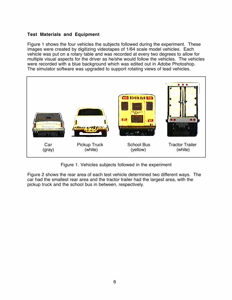
Figure 1 shows the four vehicles the subjects followed during the experiment. Theseimages were created by digitizing videotapes of 1/64 scale model vehicles. Eachvehicle was put on a rotary table and was recorded at every two degrees to allow formultiple visual aspects for the driver as he/she would follow the vehicles. The vehicleswere recorded with a blue background which was edited out in Adobe Photoshop.The simulator software was upgraded to support rotating views of lead vehicles.

Car Pickup Truck School Bus Tractor Trailer (gray) (white) (yellow) (white)

Figure 1. Vehicles subjects followed in the experiment

Figure 2 shows the rear area of each test vehicle determined two different ways. Thecar had the smallest rear area and the tractor trailer had the largest area, with thepickup truck and the school bus in between, respectively.

7

0

100

200

300

400

500

600

700

Car Pickup truck Bus Tractor trailer

Roof to Bumper Roof to Tire

Figure 2. Vehicle rear area comparison

This experiment was conducted using the UMTRI Driver Interface Research Simulator,a low-cost driving simulator based on a network of Macintosh computers (Olson andGreen, 1997). The simulator consists of an A-to-B pillar mockup of a car, a projectionscreen, a torque motor connected to the steering wheel, a sound system (to provideengine, drive train, tire, and wind noise), a sub-bass sound system (to provide verticalvibration), a computer system to project images of an instrument panel, and otherhardware. The projection screen, offering a 30 degree horizontal field of view, was 20feet (6.1 m) in front of the driver, effectively at optical infinity.

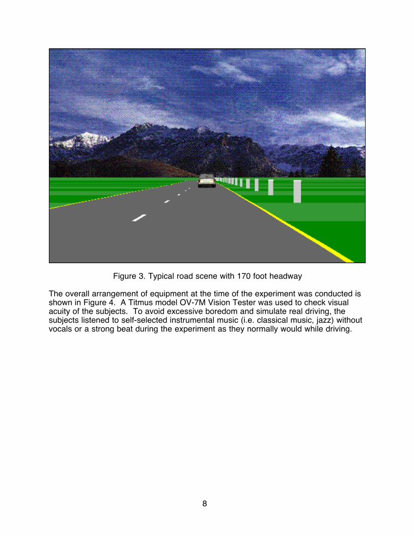
The driving environment depicted consisted of traffic signs, trees, road edge posts, andlead vehicles. Subjects drove on a 20-feet-wide, two-lane, winding road. The roadhad solid edge delineation and a dashed centerline. Appendix A provides a completegeometric description of the test roads. Figure 3 shows a typical road scene.

8

Figure 3. Typical road scene with 170 foot headway

The overall arrangement of equipment at the time of the experiment was conducted isshown in Figure 4. A Titmus model OV-7M Vision Tester was used to check visualacuity of the subjects. To avoid excessive boredom and simulate real driving, thesubjects listened to self-selected instrumental music (i.e. classical music, jazz) withoutvocals or a strong beat during the experiment as they normally would while driving.

9

36'

15'

12'

20'

1

10

3

4

5

7

6

2

9

8

14

1985 Chrysler Laser mockup with simulated hood8'X10' projection screen with 3M hi-white encapsulated reflective sheetingPMI Motion Technologies ServoDisk DC motor (model 00-01602-002 type U16M4) with Copley Controls Corp. controller (model 413) and power supply (model 645)3-spoke steering wheelSharp color LCD projection system (model XG-E850U)4"X13" plexiglas screenELO Touch Systems Intellitouch monitor (model E284A-1345)Sharp computer projection panel (model QA-1650)3M overhead projector (model 9550)Kenwood stereo cassette deck (model KX-48C), stereo graphics equalizer (model GE-7030), and AM-FM stereo receiver (model KRA-4080)Power Macintosh 9500/200Power Macintosh 7100/80AVPower Macintosh 8500/120Macintosh Quadra 840AVPanasonic GP-KS152"lipstick" CameraAlpine MRV-T300 AmplifierAura AST-1B-4 Bass ShakersBernoulli Mac Transporter 230-MB driveDell OptiPlex GXM 5166Macintosh Quadra 700Video recording systemPanasonic WV-BP510 low level light camera

1

11

131415

16

3

4

5

76

2

9

8

12

192021

17

18

10

11

16

13 22

18

18

20

22

21

17

17

12

19

15

Figure 4.Planview of simulatorlaboratory

10

Test Activities and Sequence

Subjects began by completing consent (Appendix B) and biographical forms(Appendix C), and having their vision checked. (See Appendix D for completeinstructions.) Then the subject was seated in the driving simulator. After the protocolwas described, the subject practiced driving until he/she was comfortable and wasfamiliar with the simulator handling. Then the subject drove for 6 runs of about 6 or 7minutes in length with two different vehicles to follow in each run. Specifically, thesubjects were told to "follow the vehicles as you normally would in real driving." Thefirst vehicle appeared came into sight on the road and later pulled off to the side of theroad. The second vehicle merged onto the road in view far ahead of the subject andlater came to a stop. For each steady-state portion of the following task for eachvehicle, headway, speed, and lateral position data was recorded.

The time history of the lead vehicle followed a script that specified the time when thevehicle was to accelerate or decelerate and to what speed. A copy of the script andthe equations of motion that determined the performance of the lead vehicle appear inAppendix E. The values selected were based on recommendations from vehicledyanamics experts in UMTRI's Engineering Research Division. In this experimentthere were two lead vehicle speed conditions: (1) low (mean speed 46 mi/hr (75km/hr), standard deviation 4.2 mi/hr (6.8 km/hr) and (2) high (mean speed 48 mi/hr (77km/hr), standard deviation 7.1 mi/hr (11.4 km/hr)). The slight difference in mean speedwas a design error. Figures 5 and 6 show the lead vehicle speeds for the two testconditions as a function of time.

Spe

ed (

mi/h

r)

25

30

35

40

45

50

55

60

0 50 100 150 200

Time (s)

Figure 5. Speed of lead vehicle (low variance)

11

Spe

ed (

mi/h

r)

25

30

35

40

45

50

55

60

0 50 100 150 200

Time (s)

Figure 6. Speed of lead vehicle (high variance)

Table 3 shows how the type of vehicles and their speed variance were partiallycounterbalanced across runs. The bus and the tractor trailer had low speed variabilitywhile the car and the pickup had both low and high speed variability, combinationsconsistent with their performance capabilities.

Table 3. Vehicles followed for each run

Subjects Run 1 Run 2 Run 3 Run 4 Run 5 Run 6

1,9 CC PP T B C T PP CC C P P B2,10 T C PP CC B P B T CC PP P C3,11 B T P B CC PP P C T C PP CC4,12 PP CC C P B C CC PP T B P T5,13 B C CC PP T P B C PP CC P T6,14 T B C B PP CC P T P C CC PP7,15 CC PP T P C T PP CC B P C B8,16 P T PP CC P B C B CC PP T C

Key: C = Car, P = Pickup truck, B = Bus, T = Tractor trailer,normal typeface = low speed variation, outlined typeface = high speed variation

Road curvature was intended to be varied in two ways: large and small. However, thestudent that developed the roads to be used in the simulation did not vary thecurvature of the roads. Unfortunately this mistake was caught when the data wasbeing analyzed, too late to rerun subjects.

As a secondary task, subjects also asked to call out the type of highway sign he/shedrove by: "Interstate," "U.S.," or "Michigan" (see Figure 7). The secondary task was

12

added so that the subject would not be totally focused on the lead vehicle, just as inreal driving.

Interstate U.S. Michigan

Figure 7. Road signs subjects were asked to identify while driving

After the subject had completed all test runs, subjects rated the how much each type ofvehicle blocked their vision, ranked the following distances, and rated the fidelity of thesimulator on several dimensions (Appendix F).

13

RESULTS

Data Analysis Methods and ANOVA Approach

The test data was taken from two 11,430 ft (347 m) segments from one steady-statedrive which contained two vehicle-following tasks (with breaks). Vehicle parametersincluding headway distance were sampled at a maximum of 30 Hz when the leadvehicle was far away, to a minimum of 12 Hz when the lead vehicle was closer. Forthe most part, data was collected approximately at 18 to 24 Hz. There wereapproximately 768,000 sampling periods in the entire road data set. These segmentswere taken from just after the lead vehicle merged onto the road to just before the leadvehicle pulled off the road, sections of the test sequence that should represent steadystate driving.

The simulator only collected headway data up to 600 feet (the maximum sightdistance). Drivers were not told per se to stay within the sight distance of the leadvehicle. In fact, many of the older drivers did not want to see the lead vehicle, andlagged behind so it would not be in sight (Table 4). Therefore, all headway valuesexceeding 600 feet were capped at 600 feet, skewing the data. Various alternativeswere explored to estimate the headway distance in those cases (e.g., extrapolatingfrom when vehicles were in sight), however such procedures proved to becumbersome and based on tenuous assumptions. The capped values created smallerdifferences resulting in conservative conclusions.

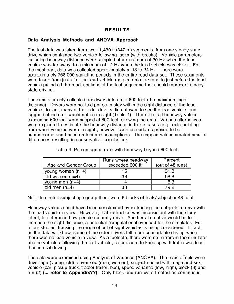
Table 4. Percentage of runs with headway beyond 600 feet.

Age and Gender GroupRuns where headway

exceeded 600 ft.Percent

(out of 48 runs)young women (n=4) 15 31.3old women (n=4) 33 68.8young men (n=4) 4 8.3old men (n=4) 38 79.2

Note: In each 4 subject age group there were 6 blocks of trials/subject or 48 total.

Headway values could have been constrained by instructing the subjects to drive withthe lead vehicle in view. However, that instruction was inconsistent with the studyintent, to determine how people naturally drive. Another alternative would be toincrease the sight distance, a potential computational overload for the simulator. Forfuture studies, tracking the range of out of sight vehicles is being considered. In fact,as the data will show, some of the older drivers felt more comfortable driving whenthere was no lead vehicle in view. As a footnote, there were no mirrors in the simulatorand no vehicles following the test vehicle, so pressure to keep up with traffic was lessthan in real driving.

The data were examined using Analysis of Variance (ANOVA). The main effects weredriver age (young, old), driver sex (men, women), subject nested within age and sex,vehicle (car, pickup truck, tractor trailer, bus), speed variance (low, high), block (6) andrun (2) (... refer to Appendix??). Only block and run were treated as continuous.

14

The model used included those seven main effects, plus the interactionsof age and vehicle, age and variance, sex with those two factors, vehicleand variance, and the sex age interaction, and that interaction withvehicle. (... hard to follow) The rationale for this choice is that sex and age ofteninteract with other characteristics, and it was important to explore those interactionswith other factors of interest. Also, given the interest in vehicle differences, vehicleinteractions were included. All other interactions were pooled into the residual errorterm.

An alternative approach explored was to consider the data piecemeal, analyzing thecar and pickup truck at two levels of speed variance in one model, and to consider allfour vehicles at low variance in another model. This approach proved to be verycomplicated and confusing when explained. An alternative approach would havebeen to treat the vehicle-variance combination as a 6-level factor, and explorevariance effects in post-hoc tests. As the data results will show, speed variance did nothave a significant effect, so separating it in this manner would have been considerableadditional work with no demonstrable benefit.

To simplify the analysis, the mean values for each subject for each run (192 total datapoints for each dependent measure) served as the unit of analysis. Again, headwaysin excess of 600 feet were assumed to be 600 feet. The measures explored includedmean headway, headway variance, lateral position, and lateral position variance.Although other measures were collected (e.g., speed, yaw angle), there was noreason they should be affected by the lead vehicle and were not explored.

What Affects Following Distance?

Following distance was significantly affected by all individual differences (age, sex,age* sex, subjects nested within sex), all at the p<0.0001 level. (See Appendix G forthe ANOVA tables.) The mean distance was 286 feet for younger drivers and 473 forolder drivers, 65 percent greater. Since the speeds driven for all conditions wereessentially identical, this also represents a 65 percent difference in time headway.Had the sight distance not been capped for older drivers, their following distancewould have been much greater. The age*sex interaction is shown in Figure 8. Noticeyounger men followed most closely (221 feet), reflecting their aggressiveness, but oldmen maintained the greatest following distance (491 feet), reflecting their diminishedcapabilities.

Differences between individuals were substantial with the estimated followingdistances varying from 134 to 490 feet. For the 490 foot case, the actual value wasprobably much large given values of only up to 600 feet were recorded. At the 45mi/hr mean speed of the lead vehicle, these distances correspond to headway times of2.0 to 7.4 s, times that are far larger than are reported for on-the-road studies (Table 1).

The impact of these characteristics is most clearly shown in the histograms of followingdistance (Figure 9). To emphasize differences in the shape of the distributions, thevertical axes have been truncated.

15

young old150

200

250

300

350

400

450

500

550

men

womenM

ean

Hea

dway

(ft)

95%tileconfidenceinterval

Figure 8. Sex * age interaction and headway

0250500750

10001250150017502000

0 100 200 300 400 500 600Headway (ft)

2418

Young women

Cou

nt

0250500750

10001250150017502000

Cou

nt

0 100 200 300 400 500 600Headway (ft)

Young men

16

0250500750

10001250150017502000

0 100 200 300 400 500 600Headway

7756

Old women

Cou

nt

0250500750

10001250150017502000

0 100 200 300 400 500 600Headway (ft)

14448

Old men

Cou

nt

Figure 9. Histograms for headway distance as a function of age and sex.

The effect of vehicle type was significant (p=.01) but variance and all other factorswere not. Figure 10 shows those effects. The main difference is that drivers followedthe car a bit closer (359 ft) than the pickup (392), bus (386), or large truck(392). Thus,although vehicle size does have some influence on following distance, the effect doesnot occur for all vehicles.

17

Bus Car Pickup Truck280

300

320

340

360

380

400

420

440

460

Low varianceHigh variance

Vehicle

Mea

n H

eadw

ay (

ft)


Figure 10. Following distances as a function of lead vehicle type

What Affects Following Distance Variability?

In a manner similar to the mean following distance, the standard deviation of headwaydistance was significantly affected by driver age (p=0.02), driver sex (p<0.0001), theage by sex interaction (p=0.02), and subject (p<0.0001). However, no other factorswere significant. Figure 11 shows the standard deviation data for the age * sexinteraction. For individual subjects, headway standard deviations ranged from 18 to93 ft. Seven of the 16 subjects were in the 50 to 80 ft range.

young old40

45

50

55

60

65

70

75

80

85

90

95

women

Age

Sta

ndar

d D

evia

tion

of H

eadw

ay (

ft)

men


18

Figure 11. Age by sex interaction for headway variability.

Figure 12 shows the headway variability data as a function of vehicle type and leadvehicle speed variance. (Confidence intervals have been omitted for clarity.) There isno explanation why the headway variance when following the car and pickup truckwere less when their speed were greater other than chance variation. The differencesare quite small (less than 1 mi/hr in one case, 4 mi/hr in the second).

Bus Car Pickup Truck58

60

62

64

66

68

70

72

74

Vehicle

Sta

ndar

d D

evia

tion

of H

eadw

ay (

ft)

Low speedvariance

High speedvariance

Figure 12. Effect of lead vehicle type and speed variance on headway variability

What Affects Mean Lateral Position?

The pronounced individual differences and need to see around a lead vehicle suggestlane placement might be affected by the lead vehicle type, although the large followingdistances reported should minimize blockage. In this case, only age, the age by sexinteraction, and subject (p<.0001) were significant. Figure 13 shows the interaction.The primary difference is that older women drove farther from the centerline (by 0.7feet) than young women. Subject means ranged from 5.3 to 6.8 to the right of thecenterline.

19

young old5.4

5.6

5.8

6

6.2

6.4

6.6

Age

Mea

n La

tera

l Pos

ition

(ft)

from

Lan

e C

ente

rline

women

men


Figure 13. Effect of age and sex on mean lateral position.

Vehicle differences were absent, will the means for all 4 vehicle types differing by lessthan 0.075 feet, less than 1 inch.

What Affects the Standard Deviation of Lateral Position?

On might speculate that the size of the lead vehicle might affect how drivers wouldfollow such a vehicle. For example, the larger the vehicle, the greater the concern formaintaining a safe following distance (with less attention devoted to maintaining laneposition). In fact, the standard deviation of lane position was affected only by sex, theage by sex interaction, and subjects nested within age and sex. Figure 14 shows thesex by age interaction. Standard deviations ranged from 0.41 to 1.18 feet. In general,young men were best and staying centered in the lane and young women had thepoorest performance. Normally, in these situations, the performance of older menwould be poorest, but there were only four subjects in each age-sex group.

20

young old.60

.65

.70

.75

.80

.85

.90

.95

1.0

1.1

Age

Sta

ndar

d D

evia

tion

of L

ater

al P

ositi

on (

ft)women

men

Figure 14. Effect of age and sex on standard deviation of lateral position

Vehicle differences were nonexistent, with the standard deviation of lateral positionranging from 0.79 ft for the bus to 0.83 ft for the car.

Subjective Evaluation of the Simulation

Subjects rated the realism of various aspects of the simulator. The overall meanresponses are found in Table 5. Most of the ratings fall between 4 and 5, indicatingthat the subjects did not find the simulation too artificial or too realistic. There were nonoticeable differences between age or gender groups. Efforts to improve the scenefidelity are in progress.

21

Table 5. Subjective rating of simulator realism.(1 to 7 scale, with 1 = very artificial and 7 = very real)

System Scale Ratingsteering effort required to operate 4.5

response time 4.9accelerator effort required to operate 4.1

response time 4.3brakes effort required to operate 5.4

response time 5.4graphics road scene 4.0

road signs 4.4lead vehicles 4.1

sound loudness 4.7pitch/tone 4.4

vibration intensity 4.7frequency 4.6

In contrast to the general trends of the data, subjects believed that they followedvehicles at a farther distance proportional to the size of the vehicle. Table 6 shows thatthe vehicle ranking for the amount of vision blockage (ranked 1 to 4) was identical tothe ranking (1 to 4) for the following distance that they thought they preferred for eachvehicle.

Table 6. Subjective ranking of vehicle size and preferred headway

Vehicle Vision Blocked Following DistanceTractor trailer 1.2 3.2Bus 2.0 3.1Pickup truck 3.0 2.1Car 3.6 1.3

The subjects were also asked what affects their following distances during real driving.Table 7 lists responses from that evaluation survey. Interestingly, visibility around thevehicle was the most commonly offered reason, even though the following distanceswere great and their was no oncoming traffic.

22

Table 7. Subjects' comments on what affects their following distances

# of timesmentioned

Comment

8 visibility around lead vehicle7 behavior of lead vehicle - speed, accelerations, erratic6 speed3 size2 type of car2 road type - curves vs. straight potions1 smell1 type of load1 "vision - slower on curves"1 avoid tailgating1 weather1 amount of traffic

Finally, as a reminder, subjects were asked to identify signs when they appeared toavoid excessive fixation on the lead vehicle. Subjects did quite well on this task,successfully identifying 1141 of 1152 signs (99% success rate). Ten signs weremissed and one was incorrectly identified.

23

CONCLUSIONS

What Affects Following Distance and Its Variability?

Following distance and its variability were primarily affected by individual differences,though following distances were less when following a car than other vehicles (byabout 30 feet, a 10% difference). For the lead vehicle speed variances examined, thatfactor had no influence on following distance. Following distances for older subjectswere 65 % greater for older subject than young subjects (473 vs. 286 feet). Headwayvariance (for 45 mi/hr) ranged from 18 to 93 ft. The extremes of the following distanceswere young men (closest) and old men (farthest). In this experiment older subjectsoften did not want to see the lead vehicle, so they often followed at in excess of themaximum sight distance in the simulator (600 feet). These values are several timeslarger than are reported in the literature for driving in traffic.

What Affects the Lateral Position and Lateral Variability of a FollowingVehicle?

Lateral position and lane variability were not expected to be affected by the nature ofthe lead vehicle, and that proved to be the case. These dependent measures wereprimarily influence by subject age, the age by sex interaction, and subject with age-sexcategory differences. Subject standard deviations ranged from 0.41 to 1.18 feet

What Are Important Considerations in Simulator-Based FollowingStudies?

It appears likely that limitations of the simulator and experiment design may haveaffected the results of this study. In order of their likely importance these include (1)the lack of following traffic, (2) constraints on the maximum sight distance, (3) updateproblems associated with close following, and (4) lead vehicle image bitmap jitter.

Since there were no mirrors in the simulator, the pressure to keep up with traffic (dueto a vehicle following the subject) was not present. The stress imposed by beingclosely followed can be considerable. In the context of the UMTRI simulator, adding amirror-based rear vision system would be a challenge given the laboratory size,though LCD displays simulating mirrors is a possibility.

Subjects were instructed to "follow the vehicles as you normally would in real driving."As a consequence, some subjects did not want to see the lead vehicle, and sometimesfollowed at a distance beyond the cutting plane of the scene generator (the maximumsight distance), here set to 600 feet. When the maximum was exceeded, the headwaywas assumed to be 600 feet. Had a larger maximum distance been used, the meanheadways would have proved to be larger. To avoid overloading the simulatorprocessor, there might be benefit in extending the cutting plane distance for the leadvehicle, but not the road scene in future studies.

Simulator update problems may also have encouraged subjects to follow at greaterthan normal distances. When driving close to a lead vehicle, the image wasnoticeably pixelated from enlargement of the scanned image bitmap of the vehicle.

24

Also, when driving close, updating the lead vehicle image bitmap decreased theupdate rate of the simulator, making it less responsive and comfortable to drive.

Finally, when closely following a lead vehicle, the change in the angular aspect wasgreater as the subject shifted their position laterally within the lane. This cause the bitmap of the lead vehicle to change, and in some situations the lead vehicle image tojitter as the bitmap alternated between two choices. Increasing headway eliminatedthis annoying jitter. Since this experiment, some changes have been made to thesoftware to change the thresholds for swapping bitmaps.

Closing Comment

For the conditions examined, the size and speed variance of the lead vehicle had littleinfluence on following behavior. However, this lack of differences may be aconsequence of the larger than normal following distances observed, distancesinfluenced by the simulator characteristics. These data contain hints there aresignificant limitations to using the UMTRI simulator as is for vehicle following studies.Some of these problems are readily resolved and steps to complete them are inprocess.

25

REFERENCES

Allen, R.W., Magdaleno, R.E., Serafin, C., Eckert, S., and Sieja, T. (1997). Driver CarFollowing Behavior Under Test Track and Open Road Driving Condition (SAE paper970170), Warrendale, PA: Society of Automotive Engineers.

Braunstein, M.L., Laughery, K.R., and Siegfried, J.B. (1963). Computer Simulation ofDriver Behavior During Car Following: A Methodological Study (Technical Report YM-1797-H-1), Buffalo, NY: Cornell Aeronautical Laboratory (available from NTIS as AD623 783).

Eberhard, C.D., Moffa, P.J., and Swihart, W.R. (1996). Taxonomy and SizeAssessment for Forward Impact Crashes Applicable to Forward Collision WarningSystems (SAE paper 961666), Warrendale, PA: Society of Automotive Engineers.

Fairclough, S. H.; May, A. J.; Carter, C. 1997. The Effect of Time Headway Feedbackon Following Behaviour, Accident Analysis and Prevention , May, 29 (3), 387-397.

Farber, E. (1995). Rear-End Collision-Warning Algorithms with Headway Warning andLead Vehicle Deceleration Information, Proceedings of the Second World Congresson Intelligent Transportation Systems , Yokohama, Japan: VERTIS, 1128-1133.

Farber, E., Freedman, M., and Tijerina, L. (1995). Reducing Motor Vehicle CrashesThrough Technology, ITS Quarterly , summer issue, 11-21.

Fenton, R.E. and Rule, R.G. (1971) On the Effects of State-Variable Feedback onDriver-Vehicle Behavior in Car Following, Symposium on Psychological Aspects ofDriver Behavior , volume 2, Applied Research, Voorburg, The Netherlands: Institute forRoad Safety Research SWOV, (paper II.1.B).

Gantzer, D. and Rockwell, T.H. (1967). Effects of Discrete Headway and RelativeVelocity Information on Car-Following Performance, Highway Research Record # 159 ,Washington, D.C.: National Academy of Sciences, Highway Research Board, 36-46.

Hattori, Y., Asano, K., Iwama, N., and Shigematsu, T. (1995). Analysis of Driver'sDecelerating Strategy in a Car-following Situation, Vehicle System Dynamics , 24,299-311.

Hirose, T., Matsumoto, S., and Inomata, S. (1976). Car-following Simulation UsingAutomobile Driving Simulator, Proceedings of the 16th International TechnicalCongress , FISITA, Tokyo, Japan: Society of Automotive Engineers of Japan, p. 6.131 -6.138.

Hoffman, E.R. and Mortimer, R.G. (1993). Drivers' Estimates of Time to Collision,Accident Analysis and Prevention , 26 (4), 511-520.

Hoffman, E.R. and Mortimer, R.G. (1994). Scaling of Relative Velocity BetweenVehicles, Proceedings of the Human Factors and Ergonomics Society 38th AnnualMeeting , Santa Monica, CA: Human Factors and Ergonomics Society, 847-851.

26

Janssen, W. and Nilsson, L. (1990). An Experiment Evaluation of In-Vehicle CollisionAvoidance Systems (DRIVE Deliverable GIDS/MAN2), Haren, the Netherlands:University of Groningen, Traffic Research Centre.

Knipling, R.R., Mironer, M. Hendricks, D.L., Tijerina, L., Everson, J., Allen, J.C., andWilson, C. (1993). Assessment of IVHS Countermeasures for Collision Avoidance:Rear-End Crashes (Technical Report DOT HS 807 995), Washington, D.C.: U.S.Department of Transportation, National Highway Traffic Safety Administration.

Knipling, R.R., Mironer, M., Hendricks, D.L., Tijerina, L., Everson, J., Allen, J.C., andWison, C. (1993). Assessment of IVHS Countermeasures for Collision Avoidance:Rear-End Crashes (Technical Report DOT HS 807 995), Washington, D.C.: U.S.Department of Transportation, National Highway Traffic Safety Administration.

Massie, D.L., Campbell, K.L., and Blower, D.F. (1993). Development of a CollisionTypology for Evaluation of Collision Avoidance Strategies, Accident Analysis andPrevention , 25 (3), 241-257.

McGehee, D.V., Dingus, T.A., Horowitz, A.D., Oberdier, L.M., and Parikh, J.S. (1993).Effect of a Headway Display on Driver Following Behavior: Experimental Field TestDesign and Initial Results, Proceedings of the Intelligent Vehicles '93 Symposium ,Tokyo, Japan: Institute of Electrical and Electronics Engineers.

Nirschl, G. and Eck, R. (1994). Driver- and Situation-Specific Effect on AssistanceSystems for Speed and Distance Control, Proceedings of the Human Factors andErgonomics Society 38th Annual Meeting , Santa Monica, CA: Human Factors andErgonomics Society, 857-861

Ota, H. (1994). Distance Headway Behavior between Vehicles from the Viewpoint ofProxemics, IATSS Research , 18 (2), 6-14.

Rockwell, T.H. and Ernst, R.L. (1965). Studies of Car Following (Technical Report202B-5), Columbus, OH: Ohio State University, Engineering Experiment Station.

Sayer, J. R.; Fancher, P. S.; Bareket, Z.; Johnson, G. E. (1995). Automatic TargetAcquisition Autonomous Intelligent Cruise Control (AICC): Driver Comfort, Acceptance,and Performance in Highway Traffic (SAE paper 950970), Warrendale, PA: Society ofAutomotive Engineers.

Schiff, W. and Oldak, R. (1990). Accuracy of Judging Time to Arrival: Effects ofModality, Trajectory, and Gender, Journal of Experimental Psychology: HumanPerception and Performance , 16 (2), 303-316.

Sleight, R. B. (1961). Effects of Instructions and Distance Judgment Aids onAutomobile Following Distance, Arlington, VA: Applied Psychology Corporation,

27

Suetomi, T., Kido, K., Yamamoto, Y., and Hata, S. (1996). A Study of CollisionWarning System Using a Moving -Base Driving Simulator, Proceedings of the SecondWorld Congress on Intelligent Transport Systems '95 , (4 ) Yokohama, Japan: VERTIS,1807-1812.

van Winsum, W. (1991). Cognitive and Normative Models of Car Driving (DRIVEDeliverable GIDS/DIA3), Haren, the Netherlands: University of Groningen, TrafficResearch Centre.

van Winsum, W. and Heino, A. (1996). Choice of Time-Headway in Car-Following andthe Role of Time-to-Collision Information in Braking, Ergonomics , 39 (4), 579-592.

Watanabe, T., Kishimoto, N., Kayafune, K., Yamada, K., and Maede, N. (1996).Development of an Intelligent Cruise Control System, Proceedings of the SecondWorld Congress on Intelligent Transport Systems , Yokohama, Japan: VERTIS, 1229-1235.

29

APPENDIX A - DESCRIPTION OF ROADS

Road 1 Road 3Length Curve Curvature Length Curve Curvature

(ft) Type (ft) (ft) Type (ft)900 Right 10000 450 Straight 0600 Straight 0 630 Left 11000480 Left 11000 1170 Right 10000840 Right 9500 600 Straight 0480 Straight 0 1140 Left 12000990 Left 13000 1260 Straight 0990 Straight 0 930 Right 9500930 Left 9500 990 Straight 0

1260 Straight 0 990 Right 130001140 Right 12000 480 Straight 0

600 Straight 0 840 Left 95001170 Left 10000 480 Right 11000

630 Right 11000 600 Straight 0450 Straight 0 900 Left 10000

Road 2 Road 4Length Curve Curvature Length Curve Curvature

(ft) Type (ft) (ft) Type (ft)900 Left 10000 450 Straight 0600 Straight 0 630 Right 11000480 Right 11000 1170 Left 10000840 Left 9500 600 Straight 0480 Straight 0 1140 Right 12000990 Right 13000 1260 Straight 0990 Straight 0 930 Left 9500930 Right 9500 990 Straight 0

1260 Straight 0 990 Left 130001140 Left 12000 480 Straight 0

600 Straight 0 840 Right 95001170 Right 10000 480 Left 11000

630 Left 11000 600 Straight 0450 Straight 0 900 Right 10000

31

APPENDIX B - CONSENT FORM

Subject: ____________ Date: _____________

Vehicle Following Study

Participant Consent Form

University of Michigan Transportation Research Institute

Human Factors Division

The purpose of this experiment is to investigate how the following distances and lanepositions of passenger cars vary as a function of the size of the lead vehicle, variationsin its speed, presentation of road signs and road curvature. During the experiment,you will drive a simulator and will simply drive behind various vehicles for severalminutes at a time while taking notice of highway signs.

The entire study will take approximately 1 hour and 40 minutes to complete. You willbe paid $20 for your participation. A few drivers experience motion discomfort whileoperating the simulator. Should you feel uncomfortable at any time and for anyreason, you may stop the experiment. You will be paid regardless.

Thank you for your help with our study. If you have any questions, please do nothesitate to ask the experimenter at any time.

The sessions will be videotaped. Do you object to being videotaped?

Yes No

I have reviewed and understand the information presented above. My participation inthis study is entirely voluntary.

Subject Signature Date

_________ Subject Name (PRINTED) Witness

Investigator: Paul Green

33

APPENDIX C - BIOGRAPHICAL FORM

Subject: ____________ Date: _____________

University of Michigan Transportation Research InstituteHuman Factors Division

Following Behavior Biographical Form

General Information

Name: __________________________________________

Sex (circle one): Male Female Age: _________

Occupation:__________________________________________________________

(If retired, please note your former occupation. If student, note your major )

Driving Experience

Are you a licensed driver (circle one)?Yes No

How many years have you been driving? __________

What kind of car do you drive the most?

Year: __________ Make: _____________ Model: ________________

Approximate annual mileage: _________________

Simulator Experience

Have you ever driven the UMTRI driving simulator? Yes No

How susceptible are you to motion sickness (circle one)?

Never Rarely Sometimes Often Don't Know

34

Driving Behavior

How aggressive a driver do you consider yourself be?

1 2 3 4 5 6 7 8 9

least mostaggressive aggressive

Suppose there are three lanes on an expressway. In which lane would you drivemost often?

Left Lane Center Lane Right Lane

Have you ever been in a collision when you rear-ended another vehicle?

Yes No

If yes, describe:

________________________________________________

_____________________________________________________________

_____________________________________________________________

Have you ever been stopped for speeding over the last 3 years?

Yes No

If Yes, how many times? ____________

How many speeding tickets did you receive? __________

1 2 3 4 5 6 7 8 9 10 11 12 13 14 T R R L T B L R L B R B T R 20/200 20/100 20/70 20/50 20/40 20/35 20/30 20/25 20/22 20/20 20/18 20/17 20/15 20/13

TITMUS VISION: (Landolt Rings) Correctivelenses worn?

Yes / No

35

APPENDIX D - EXPERIMENT INSTRUCTIONS

Experiment InstructionsDriver Behavior While Following Trucks and BusesGreat Lakes Center for Truck and Transit Research


Before Subject Arrives

Check

• sound• projector• load practice runs• change headway to 600 ft.• bass shaker

Make sure you have:• participant consent forms• biographical form• post test evaluation form• payment form and money• experiment order

Test Subject's Vision

"Please put on contacts or glasses if you use them when you drive."

Turn on both eye switches on the vision tester. Adjust the height of the visiontester for the subject. Make sure subject wears any vision correction that isworn while driving. Note on the biographical form if corrective lenses wereworn.

“Can you see in the first diamond that the top circle is complete but the otherthree are incomplete? In each diamond, tell me the location of the completecircle - top, left, right, or bottom.”

Prompt the subject until s/he has missed two in a row. Record the last numberanswered correctly on the bottom of the biographical form.

Stop test when 2 consecutive incorrect answers are given. Take the last correctanswer to be the subject’s visual acuity.

37

Introduction

Seat Subject in car and sit in front of subject

• Purpose: "The purpose of this experiment is to investigate how yourhighway following behavior while driving is affected by changing drivingconditions."

• Primary Task: "Your primary task will be to drive along a typical highwayroad while following a vehicle."

• Secondary Task: "In addition, you will have a secondary task to verballynote any highway signs you may see."

• Time: "The entire experiment will take approximately 1 hour and 40minutes."

• Pay: "You will be paid $20. You can stop anytime if you feel any discomfort.You will be paid regardless."

Hand out Consent and Biographical form

There are a few forms that we need to complete before we can begin...• Consent Form: "Please read and sign the consent form. It basically

repeats the information that I just told you."• Biographical Form: "This is the biographical form. It just asks for some

general information about yourself."• Music Selection: "You will be listening to music as you drive. Please

select a CD." (present subject with CDs)• Questions?: "If you have any questions, please feel free to ask at any

time."

Introduce subject to simulator features

• Seat Adjust: "There are seat controls located on the floor on your left."• Steering Adjust: "You can adjust the steering wheel by pulling on this

lever."• Torque Motor Warning: "The steering system will feel very much like a

real car, so simply drive as you would a real car."• Brakes and Accelerator: "The brake and the accelerator are both fully

functional."• Seat Belt: "Please wear your seat belt. The simulator will vibrate but will

not move."

38

Experiment Procedures

Introduce to the format of the experiment

• "There will be 6 driving sessions of about 6 or 7 minutes each with shortbreaks in between."

• "In each session, you will have 2 different vehicles to follow."• "Don't pass any vehicles, but you may go by a vehicle when it is going off the

road."• "You will be driving along a two lane highway. Remain in the right lane at

all times"• "Drive at or below the posted speed limit: 55 mph."• Show Signs "When you see one of these three signs, say 'Interstate,'

'Michigan,' or 'US,' corresponding to the type of sign as soon as yourecognize them. You will not need to announce speed limit signs."

• "With the exception of no passing, follow the vehicles as younormally would in real driving. Please watch your speed andremember to call out the highway signs."

Begin the Practice Run

"To get you to used to the simulator, you will now practice driving."• During the practice run, show the subject feedback of the simulator : "Now I

will have you perform some maneuvers to familiarize you with the vehiclebehavior and audio feedback. Put your left tire over the center line. Can youfeel the bumps of the center line? Now put your vehicle in the left lane of theroad. The beeping means that you are on the wrong side of the road. Itdoes not mean there is a car beeping at you. Now put your right tires on theright shoulder of the road. Can you feel the gravel?"


Begin the real run

Don't forget to: 1) Start the music2) To show elapsed time on traffic computer3) Collect data for subject4) Collect data for lead vehicles5) Write down the times of responses

"Now we can begin the experiment."

39


41

APPENDIX E - LEAD VEHICLE DYNAMICS

Script for Speed - Low Variance Condition

#truck limitations (values that follow are vehicle image identifiers)#401 Bus3b.multiLib#402 mercedes5b.multiLib#403 PickUp2b.multiLib#404 Trailer2b.multiLib

#######################################lead vehicle mergesset picture 402set location 1 34set target speed 0set speed 0set ypos 12

set target ypos 5set target speed 45

set accel 5after time 20set accel 6after time 10set accel 7after time 11set accel 0

###########################################data collection on lead 1

after location 2 20

##accel from 45 to 50 in 5 secondsset accel 7after time 5set accel 0set target speed 50

after time 4


after time 4

42

##brake from 55 to 50 in 2 secondsset brake 5after time 2set brake 0set target speed 50

after time 4


after time 10

##brake from 45 to 40 in 2.5 secondsset brake 5after time 3set brake 0set target speed 40

after time 5


after time 9


after time 4


after time 4

43


after time 4


after time 10


after time 5


after time 9


after time 4


after time 4

##brake from 55 to 50 in 2 seconds

44

set brake 5after time 2set brake 0set target speed 50

after time 4


after time 10


after time 5


###########################################lead vehicle leavesafter location 3 1set target speed 0set brake 4

Script for Speed - High Variance Condition

# first real pilot, truck limitations#401 Bus3b.multiLib#402 mercedes5b.multiLib#403 PickUp2b.multiLib#404 Trailer2b.multiLib

#######################################lead vehicle mergesset picture 403set location 1 34set target speed 0

45

set speed 0set ypos 12

set target ypos 5set target speed 45

set accel 5after time 20set accel 6after time 10set accel 7after time 11set accel 0

###########################################data collection on lead 1

after location 2 20


after time 8


after time 8


after time 9


46

after time 20


after time 7


after time 15

##accel from45 to 50 in 5 secondsset accel 7after time 5set accel 0set target speed 50

after time 8


after time 8


after time 9


after time 20

47


after time 7


###########################################lead vehicle leavesafter location 3 1set target speed 0set brake 4

after location 3 12set target ypos 20

Vehicle Acceleration Equations

Acceleration is computed as:

Acceleration = (TractiveForce - BrakeForce - RollingResistance - AscentResistance - AccelerationResistance - AerodynamicResistance) / (VehicleMass * 1.6)

Speed = Speed + Acceleration * UpdateInterval

where the UpdateInterval is usually 1/30th of a second.

The equations for the values used to compute acceleration are as follows:

TractiveForce = AcceleratorPercent * AcceleratorCoefficient TractiveForce is the force exerted by the drive wheels. AcceleratorPercent is the percent application of the accelerator pedal. AcceleratorCoefficient is a constant.

BrakeForce = BrakePercent * BrakeCoefficient BrakeForce is the force exerted by the brakes. BrakePercent is the percent application of the brake pedal. BrakeCoefficient is a constant.

48

RollingResistance = VehicleWeight * cos(VehiclePitch) * RollingCoefficient RollingResistance is the result of friction. VehicleWeight is the weight of the vehicle. VehiclePitch is the vehicle's pitch angle. RollingCoefficient is a constant.

AscentResistance = VehicleWeight * sin(VehiclePitch) AscentResistance is the force of gravity due climbing or descending hills.

AccelerationResistance = VehicleMass * Acceleration * 1.3 AccelerationResistance is the result of the vehicle's inertia. VehicleMass is the mass of the vehicle.

AerodynamicResistance = RelativeSpeed * RelativeSpeed * DragCoefficient AerodynamicResistance is aerodynamic drag. RelativeSpeed is Speed plus WindSpeed. WindSpeed is the sum of three sine waves and is intended to model variable wind speed/direction. DragCoefficient is a constant.

The default values for the various constants have changed over time and their exactvalues are not available. In general, TractiveForce, BrakeForce (when brakes wereused) and AerodynamicResistance are the dominant forces. AscentResistance is ofno consequence if there are no hills (as was the case). RollingResistance is aconstant. AccelerationResistance is only important at low speeds or during fastacceleration.

49

APPENDIX F - EVALUATION FORM

Subject: ____________ Date: _____________

Vehicle Following Study


Human Factors Division

Tractor trailer Pickup Truck School Bus Car

1) Rank the four vehicles based upon how much they blocked your vision:(1=blocked the most ... 4=blocked the least)

Tractor trailer

Pickup truck

School bus

Car

2) Rank the four vehicles based upon your preferred following distance:(1=closest ... 4=farthest)

Tractor trailer

Pickup truck

School bus

Car

3) What affects how closely you follow vehicles when you drive a real car?

50

Interstate U.S. Michigan

4) Rank these signs from easiest to most difficult to recognize while driving thesimulator (1=easiest to recognize ... 3=most difficult to recognize).

Interstate

U.S.

Michigan

5) What affects how easily you are able to recognize a sign?

51

6) Please rate the realism of UMTRI Driving Simulator:

CONTROLS

STEERING very very artificial real

Effort required to operate the steering wheel: 1 2 3 4 5 6

7

Time for road scene to respond to steering 1 2 3 4 5 67

wheel movement:

ACCELERATOR very very artificial real

Effort required to operate accelerator pedal: 1 2 3 4 5 6

7

Time for road scene to respond to accelerator 1 2 3 4 5 67

pedal movement:

BRAKE very very artificial real

Effort required to operate the brake pedal: 1 2 3 4 5

6 7

Time for road scene to respond to brake 1 2 3 4 56 7

pedal movement:

GRAPHICS

very very artificial real

Road scene appearance: 1 2 3 4 5 6

7

Road sign appearance: 1 2 3 4 5 67

Lead vehicle appearance: 1 2 3 4 5 67

52

SOUND & VIBRATION

very very artificial real

Sound loudness (engine and road sounds): 1 2 3 4 5

6 7

Sound pitch/tone (independent of loudness, 1 2 3 4 56 7 did it sound realistic?)

Vibration intensity 1 2 3 4 5 6 7

Vibration frequency (independent of intensity, 1 2 3 4 5 6 7 did it feel realistic?)

53

APPENDIX G - ANOVA TABLES

Source df Sum of Squares Mean Square F-Value P-Value

Sex 1 91692.045 91692.045 28.421 .0001Age 1 1100196.628 1100196.628 341.017 .0001Block 1 5875.220 5875.220 1.821 .1791Run 1 11193.891 11193.891 3.470 .0643Variance 1 387.661 387.661 .120 .7293Vehicle 3 35911.099 11970.366 3.710 .0129Sex * Age 1 276844.980 276844.980 85.811 .0001Sex * Vehicle 3 1721.898 573.966 .178 .9113Age * Variance 1 1115.473 1115.473 .346 .5574Age * Vehicle 3 4188.595 1396.198 .433 .7298Variance * Vehicle 1 4717.918 4717.918 1.462 .2283Subject (Sex, Age) 12 1631805.962 135983.830 42.150 .0001Sex * Age * Vehicle 3 5340.669 1780.223 .552 .6477Residual 159 512969.997 3226.226Dependent: Headway(mean)

Type III Sums of Squares


Sex 1 10330.803 10330.803 24.981 .0001Age 1 2261.000 2261.000 5.467 .0206Block 1 65.901 65.901 .159 .6903Run 1 3.469 3.469 .008 .9271Variance 1 175.024 175.024 .423 .5163Vehicle 3 1862.425 620.808 1.501 .2164Sex * Age 1 2524.986 2524.986 6.106 .0145Sex * Vehicle 3 7087.722 2362.574 5.713 .0010Age * Variance 1 28.976 28.976 .070 .7916Age * Vehicle 3 650.034 216.678 .524 .6664Variance * Vehicle 1 60.296 60.296 .146 .7031Subject (Sex, Age) 12 93867.855 7822.321 18.915 .0001Sex * Age * Vehicle 3 560.707 186.902 .452 .7163Residual 159 65753.522 413.544Dependent: Headway(SD)


54


Sex 1 .255 .255 3.070 .0817Age 1 3.887 3.887 46.748 .0001Block 1 .026 .026 .311 .5779Run 1 .145 .145 1.740 .1891Variance 1 .038 .038 .455 .5009Vehicle 3 .105 .035 .420 .7392Sex * Age 1 6.365 6.365 76.561 .0001Sex * Vehicle 3 .242 .081 .971 .4079Age * Variance 1 .019 .019 .232 .6310Age * Vehicle 3 .104 .035 .418 .7402Variance * Vehicle 1 .025 .025 .305 .5813Subject (Sex, Age) 12 27.930 2.327 27.994 .0001Sex * Age * Vehicle 3 .449 .150 1.799 .1495Residual 159 13.219 .083Dependent: YPos(mean)



Sex 1 .543 .543 15.598 .0001Age 1 .024 .024 .680 .4107Block 1 .003 .003 .092 .7617Run 1 .017 .017 .476 .4912Variance 1 .029 .029 .829 .3639Vehicle 3 .016 .005 .155 .9264Sex * Age 1 1.987 1.987 57.065 .0001Sex * Vehicle 3 .022 .007 .214 .8865Age * Variance 1 .015 .015 .444 .5063Age * Vehicle 3 .014 .005 .133 .9405Variance * Vehicle 1 .057 .057 1.628 .2039Subject (Sex, Age) 12 3.440 .287 8.235 .0001Sex * Age * Vehicle 3 .048 .016 .460 .7103Residual 159 5.535 .035Dependent: YPos(SD)


herbert yoo and paul green - university of michigandriving/publications/umtri-99-14.pdffinal, 9/94 -...

Documents