harries corner detector derived by local autocorrelation function (survey)

HARRIES CORNER DETECTOR DERIVED BY LOCAL

AUTOCORRELATION FUNCTION (SURVEY)

Angu Ramesh B

Final year M.E (Medical Electronics), SXCCE, TN, INDIA

Mail: [email protected], Mobile: +918056723334

Harries operator is nothing but a corner detector in a digital image, which is

based on interest point detection. We should easily recognize the point by looking at

intensity values within an image and we can able to absolves the change of

Appearance in Neighborhood of a pixel obtained and the feature extracted with

respect to intensity pattern, so there is a possibility for incorporating either spatial and

geometrical information

In computer vision, usually we need to find matching points between different

frames of an environment. Due to know how two images relate to each other, we can

use both images to extract information of them. When we say matching points we are

referring, in a general sense, to characteristics in the scene that we can recognize easily.

We call these characteristics features such as flat regions, edges, corners (interest

points) which is shown in the figure 3.2 and figure 3.3. Corners are special than

remaining two because, since it is the intersection of two edges, it represents a point in

which the directions of these two edges change. Hence, the gradient of the image (in

both directions) have a high variation, which can be used to detect it.

3.2 EQUATION EXPLANATION

Since corners represents a variation in the gradient in the image, we will look for

this “variation”. Consider a grayscale image . We are going to sweep a

window (with displacements in the x direction and in the right

direction) and will calculate the variation of intensity.

(3.1)

mailto:[email protected]

Where:

is the window at position

is the intensity at

is the intensity at the moved window

Since we are looking for windows with corners, we are looking for windows

with a large variation in intensity. Hence, we have to maximize the equation above,

specifically the term:

(3.2)

Using Taylor expansion:

(3.3)

Expanding the equation and cancelling properly:

(3.4)

Which can be expressed in a matrix form as:

(3.5)

Let’s denote:

(3.6)

So, our equation now is:

(3.7)

A score is calculated for each window, to determine if it can possibly contain a

corner:

(3.8)

where:

det(M) =

trace(M) =

a window with a score greater than a certain value is considered a “corner

Figure 3.2(Corner Edge response.1) Figure 3.3(Corner Edge response.2)

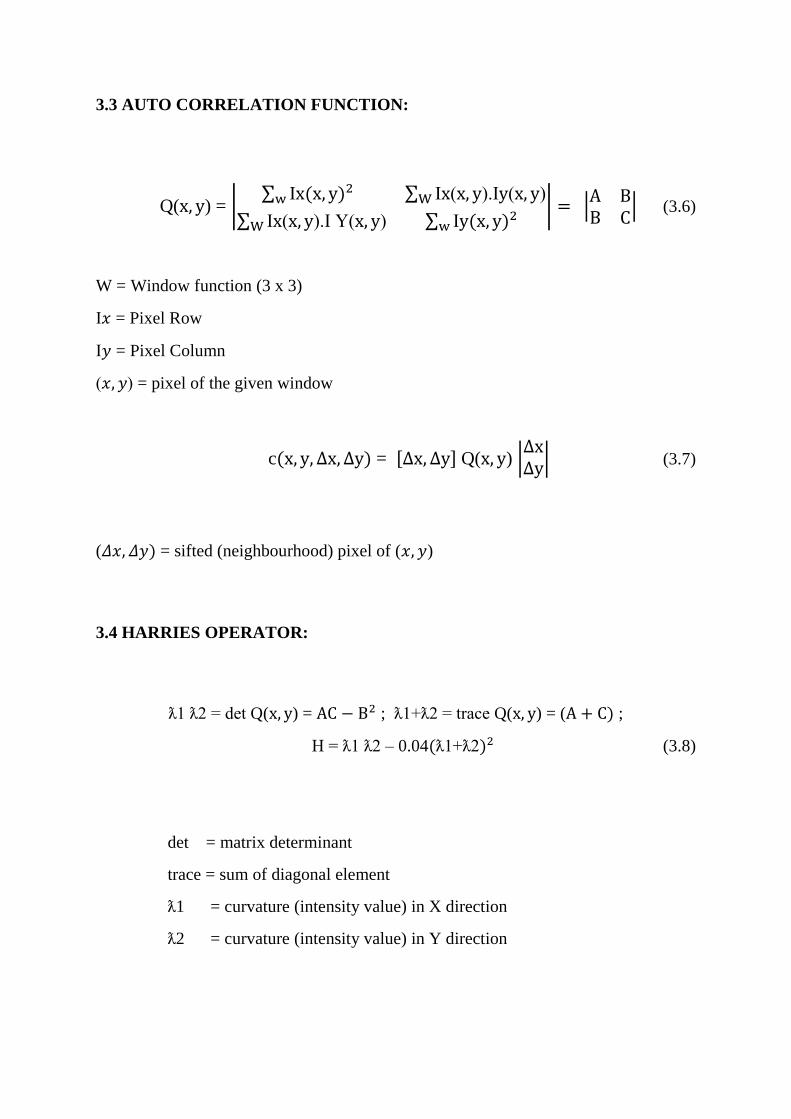
3.3 AUTO CORRELATION FUNCTION:

Q(x, y) = |∑ Ix(x, y)2w ∑ Ix(x, y).Iy(x, y)W

∑ Ix(x, y).I Y(x, y)W ∑ Iy(x, y)2w | = |

A BB C

| (3.6)

W = Window function (3 x 3)

I𝑥 = Pixel Row

I𝑦 = Pixel Column

(𝑥, 𝑦) = pixel of the given window

c(x, y, Δx, Δy) = [Δx, Δy] Q(x, y) |ΔxΔy

| (3.7)

(𝛥𝑥, 𝛥𝑦) = sifted (neighbourhood) pixel of (𝑥, 𝑦)

3.4 HARRIES OPERATOR:

ƛ1 ƛ2 = det Q(x, y) = AC − B2 ; ƛ1+ƛ2 = trace Q(x, y) = (A + C) ;

H = ƛ1 ƛ2 – 0.04(ƛ1+ƛ2)2 (3.8)

det = matrix determinant

trace = sum of diagonal element

ƛ1 = curvature (intensity value) in X direction

ƛ2 = curvature (intensity value) in Y direction

3.5 OVERALL BLOCK DIAGRAM OF HARRIS OPERATOR

Figure: 3.4 (Overall Block Diagram of Harris Operator)

RESULT AND DISCUSSION

For a human, it is easier to identify a “corner”, but a mathematical detection is

required in case of algorithms. Chris Harris and Mike Stephens in 1988 improved upon

Moravec's corner detector by taking into account the differential of the corner score

with respect to direction directly instead of using shifted patches. Moravec only

considered shifts in discrete 45 degree angles whereas Harris considered all directions.

Harris detector has proved to be more accurate in distinguishing between edges

and corners. In this a circular Gaussian window is used to reduce noise and local

autocorrelation function is used for find out the correlation between the original position

and sifted position. Harris equation provides the both Eigen values of x and y direction,

when the both Eigen values are larger that’s become corner or interest points, when only

any one of Eigen values of x and y direction are larger that’s become edges, and both

Eigen values are become low, that’s become flat region. Here by the feature has been

extracted with respect to intensity pattern

In this section we are computing some test images and medical images as a X

direction [A(x,y)], Y direction [C(x,y)], Diagonal direction [B(x,y)] and also corner

detected images with their corresponding input image [I(x,y)] are shown in the

figure:3.4.

4.1 OUTPUT

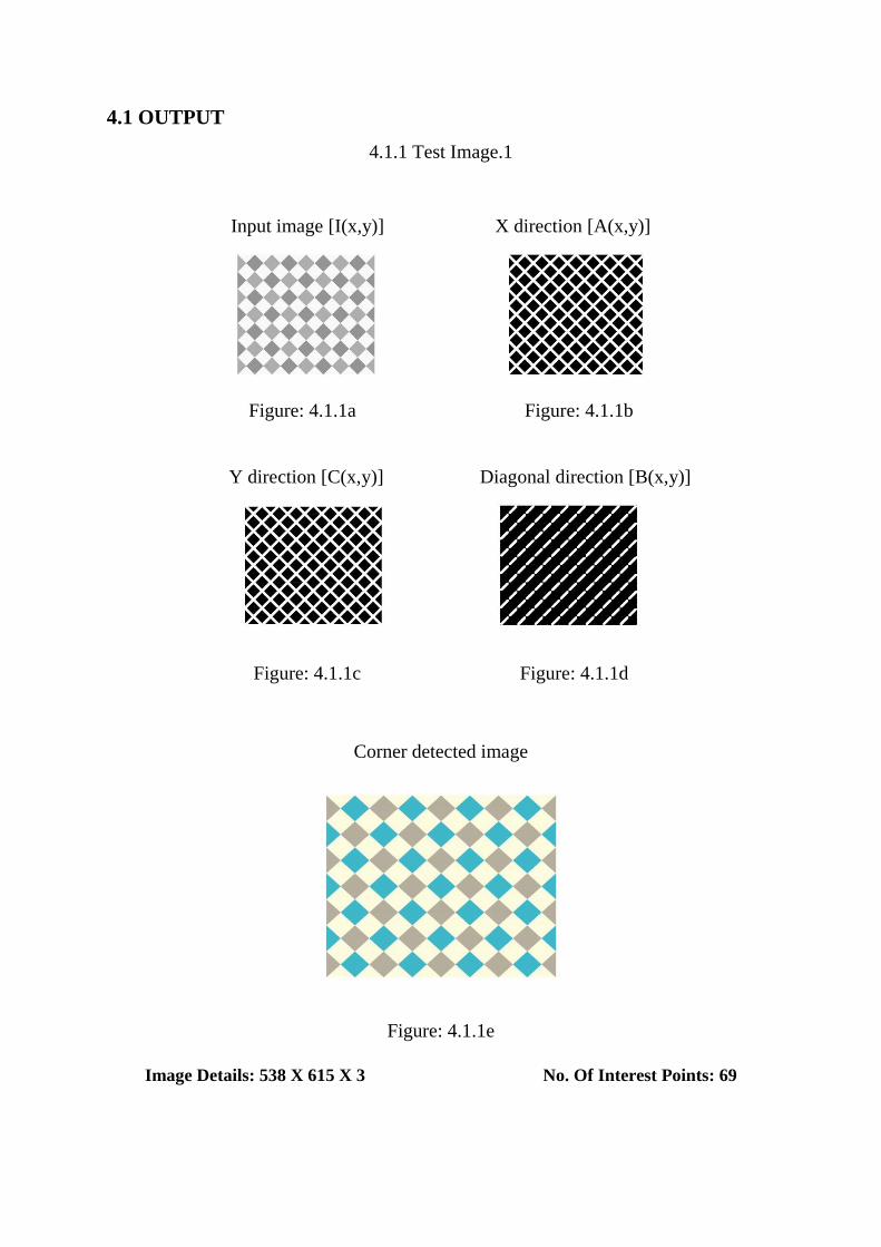
4.1.1 Test Image.1

Input image [I(x,y)] X direction [A(x,y)]

Figure: 4.1.1a Figure: 4.1.1b

Y direction [C(x,y)] Diagonal direction [B(x,y)]

Figure: 4.1.1c Figure: 4.1.1d

Corner detected image

Figure: 4.1.1e

Image Details: 538 X 615 X 3 No. Of Interest Points: 69

4.1.2 Test Image.2






Figure: 4.1.2e


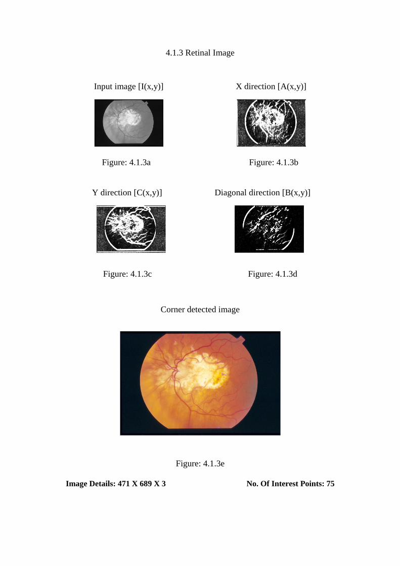
4.1.3 Retinal Image






Figure: 4.1.3e


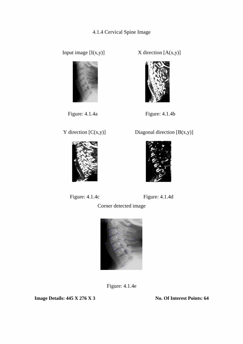
4.1.4 Cervical Spine Image






Figure: 4.1.4e


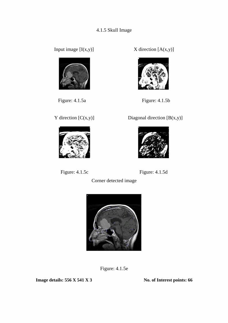
4.1.5 Skull Image






Figure: 4.1.5e

Image details: 556 X 541 X 3 No. of Interest points: 66

CONCLUSION

The image features are extracted with respect to the intensity pattern of the image

using harries corner detector which is derived by the local autocorrelation function.

Here by the system can able to achieve the spatial and geometrical information during

the similarity measurement processes

For an example, here I take 2 retinal images for registration and extracted the

features like interest points (corners) with respect to intensity pattern. Image1 has 75

interest points and image2 has 79 interest points. This points are used to labelling the

high intensity regions of the two images which can be used to find out the similarity

between the images

harries corner detector derived by local autocorrelation function (survey)

Education