harmony filter: a robust visual tracking system using the improved harmony search algorithm

Image and Vision Computing 28 (2010) 1702–1716

Contents lists available at ScienceDirect

Image and Vision Computing

j ourna l homepage: www.e lsev ie r.com/ locate / imav is

Harmony filter: A robust visual tracking system using the improved harmonysearch algorithm

Jaco Fourie a,b,⁎, Steven Mills b, Richard Green a

a Computer Science and Software Engineering, University of Canterbury, Christchurch, New Zealandb Geospatial Research Centre (NZ) Ltd, Christchurch, New Zealand

⁎ Corresponding author. Computer Science and SoftwCanterbury, Christchurch, New Zealand.

E-mail address: [email protected] (J. Fourie).

0262-8856/$ – see front matter © 2010 Elsevier B.V. Adoi:10.1016/j.imavis.2010.05.006

a b s t r a c t
a r t i c l e i n f o
Article history:Received 14 May 2009Received in revised form 6 May 2010Accepted 22 May 2010

Keywords:Visual trackingHarmony search algorithmSoft computingEvolutionary algorithm 2000 MSC: 68T45

In this article a novel approach to visual tracking called the harmony filter is presented. It is based on theHarmony Search algorithm, a derivative free meta-heuristic optimisation algorithm inspired by the waymusicians improvise new harmonies. The harmony filter models the target as a colour histogram andsearches for the best estimated target location using the Bhattacharyya coefficient as a fitness metric.Experimental results show that the harmony filter can robustly track an arbitrary target in challengingconditions. We compare the speed and accuracy of the harmony filter with other popular tracking algorithmsincluding the particle filter and the unscented Kalman filter. Experimental results show the harmony filter tobe faster and more accurate than both the particle filter and the unscented Kalman filter.

are Engineering, University of

ll rights reserved.

© 2010 Elsevier B.V. All rights reserved.

1. Introduction

The ability to track an arbitrary object through a video sequence isimportant in many applications including augmented reality [1],video compression [2] and driver assistance [3]. When only visualinformation from a camera is used to accomplish this, the problem isknown as visual tracking. The process is complicated by the fact thatthe tracker's target can only be approximately represented using ourlimited information. System noise that is always present whenworking with real video data further decreases our ability to ac-curately recognise the target in every video frame.

In the past researchers performed visual tracking using a variety ofmethods and algorithms. One of themost popular remains the Kalmanfilter and its extensions [4,5]. In the original Kalman filter thedistribution of the target location was assumed to be Gaussian. Thisapproximation caused the algorithm to be less robust in ambiguousenvironments or in situations where the target is tracked throughvisual clutter. In an attempt to improve robustness various adaptionshave been made to the original Kalman filter including the extendedKalman filter (EKF) and the unscented Kalman filter (UKF) [4].

One of the most successful algorithms for visual tracking is theparticle filter algorithm introduced by Isard and Blake [6]. The particlefilter algorithm is an importance sampling method and is also knownas a sequential Monte Carlo method due to the Monte Carlo samplingstep that forms its basis. The particle filter can accurately model non-Gaussian distributions and is more robust in visual clutter than

Kalman filter based methods. However, to accurately model complexnon-Gaussian distributions, the particle filter requires significantcomputational resources that may not be available.

Recently, researchers have started to investigate evolutionaryalgorithms as an alternative way to perform visual tracking. Mostapproaches involve the use of genetic algorithms or the particleswarm optimisation algorithm [7–10]. The advantage of thesemethods is that no assumptions are made about the shape of thedistribution or the noise in the system. This gives the methods thepotential for accurate solutions even in challenging ambiguousenvironments. However, the improved accuracy often comes at acost of increased computational resources.

The purpose of this study is to investigate a new evolutionaryalgorithm called Harmony Search as an algorithm to perform visualtracking. Harmony Search is a meta-heuristic evolutionary algorithmbased on the way musicians improvise to find optimal harmony in aperformance [11]. The algorithm has been demonstrated in civil,mechanical, and electrical engineering as an efficient optimisationalgorithm that often finds a solution faster than genetic algorithms orneural network based algorithms could [12,13]. It has also proved tobe very successful in many other diverse fields including computervision, image segmentation, vehicle routing and music composition[14–18]. We show that Harmony Search can be used as a robust andcomputationally inexpensive algorithm for performing visualtracking.

We develop the harmony filter algorithm by first defining how thevisual tracking problem can be interpreted as an optimisationalgorithm. Once the value to be optimised has been defined anappropriate cost function to evaluate possible solutions is given. TheHarmony Search algorithm is then used to optimise solution vectors

http://dx.doi.org/10.1016/j.imavis.2010.05.006

mailto:[email protected]

http://dx.doi.org/10.1016/j.imavis.2010.05.006

http://www.sciencedirect.com/science/journal/02628856

1703J. Fourie et al. / Image and Vision Computing 28 (2010) 1702–1716

using the cost function until the system converges to the best solution.We show that this can be done in real-time and compare its speed andaccuracy with other popular methods including the particle filter andthe unscented Kalman filter (UKF).

We build on our previous research [15] and offer a more detailedexposition in this article. An expanded analysis is also provided andmore extensive results are presented.

In the next section we investigate current state-of-the-art meth-ods for visual tracking. We note the limitations of these systems andindicate the assumptions that are made and the effect these have oneach method's performance. In Section 3 Harmony Search is in-troduced and some extensions to the original algorithm are in-vestigated. Section 4 gives an overview of the harmony filter'sarchitecture. Detailed implementation details are then given andcertain aspects of the design are discussed. The section concludes withan analysis of the parameter sensitivity of the system and a discussionon the overall computational complexity of the algorithm. In Section 5we compare the harmony filter with other popular algorithms forperforming visual tracking and discuss the results. We conclude thearticle in Section 6 and identify future research directions that stemfrom this study.

2. Related work

The Kalman filter is one of the earliest algorithms successfully usedin visual tracking. Gutman et al. published a paper in 1990 detailing ageneric tracking scheme that could track targets with varying dy-namics using the Kalman filter [4]. Since then researchers have mademuch progress adapting and improving the Kalman filter for tracking,with one of the most successful extensions being the unscentedKalman filter [19].

Issard et al. published the Condensation algorithm in 1997 andintroduced the first application of the particle filter algorithm to visualtracking [6]. Condensation proved to be superior to the Kalman filterin tracking curves through environments cluttered with local dis-tractors. It also showed that stochastic importance sampling methodscan be used when real-time performance is required.

By efficiently combining a number of methods Nummiaro et al.designed a fast and robust tracking system also based on the particlefilter [20]. This method uses colour histograms as a target model andformulates the problem in such a way that gradient based opti-misation algorithms can be used to perform target localisation. TheBhattacharyya coefficient is used to measure the similarity betweenhistograms and acts as the fitness metric when optimisation algo-rithms are used. It is defined as

Bðt; cÞ = ∑N

i=1

ffiffiffiffiffiffiffiffiffiffiffiffiffiffiffitðiÞcðiÞ

q;

where N is the number of bins in the histograms and t and c are thehistograms being compared. It was shown that this approach givessuperior performance during large scale changes in the target orduring rapid and erratic movement.

The use of colour histograms as a target model in trackingapplicationswas explored bymany researchers. Chen et al. introducedthe Adaptive Color Vision System (ACVS) that uses adaptive colourhistogram models that automatically update themselves to adaptto changing light conditions [21]. The models adapt by learning adistribution of colours through various light conditions and using thisdistribution rather than the original histogramas the targetmodel. Thehistogram back projection method, used to robustly recognise objectsin an image, is then used to match targets with models [22]. Thismethod works well in maintaining robust target acquisition throughchanging light conditions but fails when similarly coloured objects tothe target enter the frame. This is due to the target model adapting to

match objects from a range of similar colours in order to be robustduring lighting changes.

Comaniciu et al. proposed a visual tracking method that usescolour histograms and formulates the problem in such a way thatgradient based optimisation algorithms can be used to perform targetlocalisation [23]. This method also uses the Bhattacharyya coefficientto measure the similarity between histograms [24]. It creates asmooth evaluation function that is optimised using the mean shiftprocedure. Various optimisations regarding the computational com-plexity of the algorithm was made resulting in a system that is able toperform real-time tracking robustly in environments containingvisual clutter. This method proved to be robust under partial occlusionand was able to maintain target localisation during erratic motion andchanging light conditions. It effectively showed that colour histo-grams contain enough information for robust target localisation andthat the Bhattacharyya coefficient is an efficient metric with which toformulate visual tracking as an optimisation problem.

By showing that visual tracking can be achieved efficiently usinggradient based optimisation algorithms researchers started investi-gating optimisation algorithms that are popular in other fields such asthe genetic algorithm and the particle swarm optimisation (PSO)algorithm. Sulistijono et al. proposed a method using PSO for a headtracking application [9]. This is a completely different approach to theones previously mentioned and does not use colour histograms torepresent targets. Instead, template matching with a previouslyconstructed head template is used to define the function to beoptimised. PSO or a genetic algorithm is then used to optimise thisfunction in order to correctly localise the head tracker. The headtemplate is simply an image of a generic head indicating where hairand skin coloured pixels are expected to be found. Performancecomparisons between the PSO and genetic algorithm implementa-tions show that the genetic algorithm tends to converge to a morestable solution but that PSO is faster. Both algorithms can be adjustedto favour speed over accuracy by limiting the number of functionevaluations until convergence.

Zang et al. also showed that the PSO algorithm can be successfullyapplied to visual tracking [10]. In their work the PSO algorithm isadapted specifically for use in visual tracking. The parameters thatcontrol the movement of the particles in the swarm is updateddynamically depending on the fitness values of the particles. In thisway the temporal continuity information of the sequence is taken intoaccount resulting in improved accuracy and robustness. It was alsoshown theoretically that this framework could be interpreted as amulti layer importance sampling based particle filter. Experimentalresults showed that this PSO based tracking system ismore robust andeffective than state-of-the-art particle filter and unscented particlefilter based tracking systems especially during fast and erratic motion.

Minami et al. used a genetic algorithm to design a visual servingsystem that is able to recognise and track a target, in this case a fish,using only a grey-scale image [7]. They employ an elitist selectionstrategy in the genetic algorithm that maintains the best individualsolution throughout all generations. This is similar to the strategy ofPSO that constantly keeps track of the best solution in the population.The genetic algorithm is used to optimise a function that minimisesthe difference between a previously defined fish template and theimage captured by the camera. The evaluations function used tomeasure this distance is not related to the Bhattacharyya coefficientbut is similar to template matching used by Sulistijono et al. Thesystem proved successful in recognising and robustly tracking a fishtarget in real-time using limited amounts of computational resources.

The following observations can be made from the six visualtracking systems that were investigated. Firstly, fast and robusttracking can be achieved using colour histograms and the Bhattachar-yya coefficient. Also, fast and accurate optimisation of the resultingfitness function can be achieved using evolutionary algorithms. This isdue to the algorithm's ability to sacrifice accuracy for speed by forcing

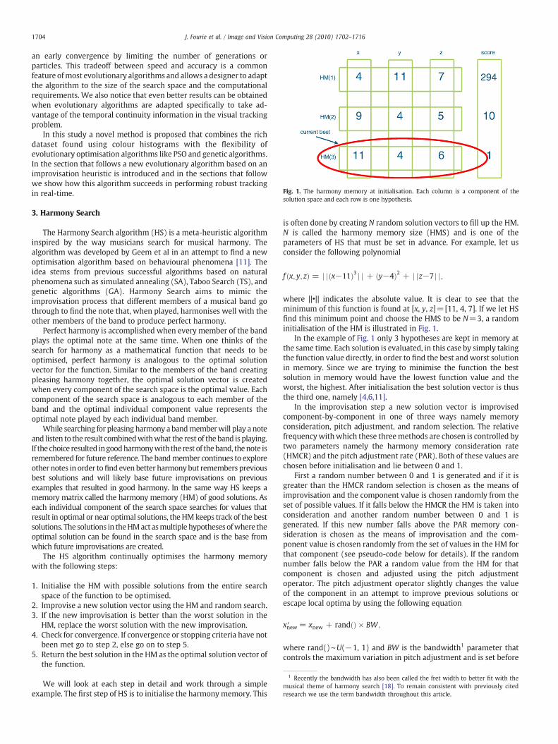
Fig. 1. The harmony memory at initialisation. Each column is a component of thesolution space and each row is one hypothesis.

1 Recently the bandwidth has also been called the fret width to better fit with themusical theme of harmony search [18]. To remain consistent with previously citedresearch we use the term bandwidth throughout this article.

1704 J. Fourie et al. / Image and Vision Computing 28 (2010) 1702–1716

an early convergence by limiting the number of generations orparticles. This tradeoff between speed and accuracy is a commonfeature ofmost evolutionary algorithms and allows a designer to adaptthe algorithm to the size of the search space and the computationalrequirements. We also notice that even better results can be obtainedwhen evolutionary algorithms are adapted specifically to take ad-vantage of the temporal continuity information in the visual trackingproblem.

In this study a novel method is proposed that combines the richdataset found using colour histograms with the flexibility ofevolutionary optimisation algorithms like PSO and genetic algorithms.In the section that follows a new evolutionary algorithm based on animprovisation heuristic is introduced and in the sections that followwe show how this algorithm succeeds in performing robust trackingin real-time.

3. Harmony Search

The Harmony Search algorithm (HS) is a meta-heuristic algorithminspired by the way musicians search for musical harmony. Thealgorithm was developed by Geem et al in an attempt to find a newoptimisation algorithm based on behavioural phenomena [11]. Theidea stems from previous successful algorithms based on naturalphenomena such as simulated annealing (SA), Taboo Search (TS), andgenetic algorithms (GA). Harmony Search aims to mimic theimprovisation process that different members of a musical band gothrough to find the note that, when played, harmonises well with theother members of the band to produce perfect harmony.

Perfect harmony is accomplished when every member of the bandplays the optimal note at the same time. When one thinks of thesearch for harmony as a mathematical function that needs to beoptimised, perfect harmony is analogous to the optimal solutionvector for the function. Similar to the members of the band creatingpleasing harmony together, the optimal solution vector is createdwhen every component of the search space is the optimal value. Eachcomponent of the search space is analogous to each member of theband and the optimal individual component value represents theoptimal note played by each individual band member.

While searching for pleasing harmony a bandmemberwill play a noteand listen to the result combinedwithwhat the rest of the band is playing.If the choice resulted ingoodharmonywith the rest of theband, thenote isremembered for future reference. The bandmember continues to exploreother notes in order tofind even better harmonybut remembers previousbest solutions and will likely base future improvisations on previousexamples that resulted in good harmony. In the same way HS keeps amemory matrix called the harmony memory (HM) of good solutions. Aseach individual component of the search space searches for values thatresult in optimal or near optimal solutions, the HMkeeps track of the bestsolutions. The solutions in theHMact asmultiple hypotheses ofwhere theoptimal solution can be found in the search space and is the base fromwhich future improvisations are created.

The HS algorithm continually optimises the harmony memorywith the following steps:

1. Initialise the HM with possible solutions from the entire searchspace of the function to be optimised.

2. Improvise a new solution vector using the HM and random search.3. If the new improvisation is better than the worst solution in the

HM, replace the worst solution with the new improvisation.4. Check for convergence. If convergence or stopping criteria have not

been met go to step 2, else go on to step 5.5. Return the best solution in the HM as the optimal solution vector of

the function.

We will look at each step in detail and work through a simpleexample. The first step of HS is to initialise the harmonymemory. This

is often done by creating N random solution vectors to fill up the HM.N is called the harmony memory size (HMS) and is one of theparameters of HS that must be set in advance. For example, let usconsider the following polynomial

f ðx; y; zÞ = j j ðx−11Þ3 j j + ðy−4Þ2 + j jz−7 j j ;

where ||•|| indicates the absolute value. It is clear to see that theminimum of this function is found at [x, y, z]=[11, 4, 7]. If we let HSfind this minimum point and choose the HMS to be N=3, a randominitialisation of the HM is illustrated in Fig. 1.

In the example of Fig. 1 only 3 hypotheses are kept in memory atthe same time. Each solution is evaluated, in this case by simply takingthe function value directly, in order to find the best andworst solutionin memory. Since we are trying to minimise the function the bestsolution in memory would have the lowest function value and theworst, the highest. After initialisation the best solution vector is thusthe third one, namely [4,6,11].

In the improvisation step a new solution vector is improvisedcomponent-by-component in one of three ways namely memoryconsideration, pitch adjustment, and random selection. The relativefrequencywithwhich these threemethods are chosen is controlled bytwo parameters namely the harmony memory consideration rate(HMCR) and the pitch adjustment rate (PAR). Both of these values arechosen before initialisation and lie between 0 and 1.

First a random number between 0 and 1 is generated and if it isgreater than the HMCR random selection is chosen as the means ofimprovisation and the component value is chosen randomly from theset of possible values. If it falls below the HMCR the HM is taken intoconsideration and another random number between 0 and 1 isgenerated. If this new number falls above the PAR memory con-sideration is chosen as the means of improvisation and the com-ponent value is chosen randomly from the set of values in the HM forthat component (see pseudo-code below for details). If the randomnumber falls below the PAR a random value from the HM for thatcomponent is chosen and adjusted using the pitch adjustmentoperator. The pitch adjustment operator slightly changes the valueof the component in an attempt to improve previous solutions orescape local optima by using the following equation

xnew′ = xnew + randðÞ × BW;

where rand()∼U(−1, 1) and BW is the bandwidth1 parameter thatcontrols the maximum variation in pitch adjustment and is set before


initialisation. The pitch adjustment operator is similar to the mutationoperator found in genetic algorithms.

DefineM as the number of components in the search space and UBiand LBi as the upper and lower bound value of the ith component. LetU(0, 1) be a random number between 0 and 1 generated from auniform distribution. The pseudo-code for the improvisation processis then given as follows.

for each i∈ [1, M] doif U(0, 1)NHMCR then {random selection}

xi′←LBi+r×(UBi−LBi)where r∼U(0, 1)

else {memory consideration}xi′←xi

jwhere j∼U(1, HMS)

if U(0, 1)≤PAR then {pitch adjustment}xi′←xi′+r×BW where r∼U(−1, 1)

end ifend if

end for

An example of all three improvisation methods being used togenerate a new solution vector is illustrated in Fig. 2. The first com-ponent, x, is generated using memory consideration. This means thatthe x-value of the new improvisation has to be ∈{4, 9, 11} and in thiscase 11 was chosen. The second component, y, is improvised usingpitch adjustment. The value from the second solution vector (4) wasselected and as small random offset applied to create the improvisedvalue of 5. The third component, z, is improvised using randomselection and can be any value in the set of all possible values for z inthe search space. As seen in the example, the value does not need to bepresent in the HM and in this case the value 12 was chosen.

The new improvised vector is now evaluated and compared withthe worst solution in the HM. Since the new improvisation, [5,11,12],evaluates to a lower score, which is better since we are minimising, itreplaces the vector [4,7,11] that was the worst vector in the HM.Notice that after the HM is updated that the worst solution is notnecessarily the new improvisation but can be any vector in the HM. Inthis case the new worst is the second vector, [4,5,9].

After improvisation the convergence and stopping criteria arechecked. These come in many forms and are often problem specific.The easiest stopping criteria is simply to stop after a set number ofimprovisations. The designer might decide that after 1000 improvisa-tions the best solution in the HM is close enough to the optimalsolution. It often happens, however, that HS found this point after only

Fig. 2. A new improvised solution vector. The new improvisation is better than theworst solution in the HM and will thus replace it.

200 improvisations and that no progress was made in the last 800improvisations. When real-time operation is important this situationhas to be detected so the algorithm can be terminated early and notime is wasted on improvisations that make no improvements.

One way to detect this is to consider the algorithm convergedwhen after C improvisations no change in the HM was made. Theparameter C has to be chosen carefully to minimise wasted im-provisations while at the same time not causing the algorithm toprematurely converge when significant improvements can still bemade. A safer way to detect convergence might be to measure thedistance between the best and worst solution in the HM. If thisdistance is sufficiently small it means that the algorithm converged toa single point in the search space and has probably converged. Thedanger of this approach is that HS could temporarily be stuck in a localoptimum but will eventually escape given enough time. This makes itappear to be converged when it is really not. When consideringstopping and convergence criteria the best approach seems to be acombination of many methods manually tailored to the specific pro-blem through experimentation.

It is important to realise that these methods for detecting con-vergence are heuristic just like the main algorithm and that accuratedetection cannot be guaranteed. Even though a combination of thesemethods generally give excellent results, there are instances wherethe algorithm runs the maximum number of iterations even thoughimprovement of the solution has stopped earlier.

The primary parameters of the Harmony Search algorithm, asmentioned in the preceding paragraphs, are as follows. The harmonymemory size (HMS) controls the number of hypotheses that are keptin memory simultaneously. It is usually kept small (b10) to ensurequick convergence but can cause the algorithm to become easilytrapped in local optima when chosen too small. The HMS is usuallytuned to the size of the search space and the number of components.

The harmony memory consideration rate (HMCR) controls theamount of random search. This is usually kept high (N0.8) in order toencourage memory consideration and is usually set to favour con-vergence over exploration. When the function contains many localoptima and the HM is initialised using random solution vectors theHMCR is usually set slightly lower to make sure the search space isproperly explored and local optima are avoided.

The pitch adjustment rate (PAR) and bandwidth (BW) parameterswork together to either favour accurate but slower convergence orquick convergence to approximated optima. When the PAR is highand the BW is small, many solutions close to existing hypotheses areexplored. This will cause accurate solutions to be found when thehypotheses in the HM are all in the basis of attraction of some optimalpoint. This is made at the expense of quick exploration and as the BWbecomes smaller, the convergence will become slower.

3.1. The improved harmony search algorithm

The improved harmony search algorithm (IHS) was developed byMahdavi et al. and enhances the original HS algorithm by automat-ically fine tuning the PAR and BW parameters [13]. In the original HSalgorithm the PAR and BW parameters must be chosen by thedesigner and it is often difficult to knowwhat their value should be togive the fastest possible convergence at the required accuracy. Withthe IHS algorithm the designer only has to specify a minimum andmaximum possible value for both the PAR and the BW.

The key insight that led to IHS is that the value of the PAR and theBW has to change dynamically depending on how long the algorithmhas been optimising. At the beginning of the optimisation processpriority has to be given to thoroughly exploring the search space andthe largest possible diversity of solutions are sought after in the HM.This can be accomplished by a small PAR that favours memory con-sideration over pitch adjustment and a large BW that favours largedeviations from the original.

image of Fig.�2


Similarly, near the end of the convergence process priority must begiven to tight and accurate convergence and it is assumed that thehypotheses in theHMare already in thebasis of attraction of the optimalpoint. The best way to accomplish this is to keep the PAR large toencourage pitch adjustment and the BW small for maximum accuracy.

This strategy of continually updating the value of the PAR and BWis implemented in IHS by recalculating the PAR and BW at everyiteration using the following equations.

PARðiÞ = PARmin +PARmax−PARmin

NI⋅ i

BWðiÞ = BWmaxeðk⋅iÞ

k =ln BWmin

BWmax

� �

NI;

where PARmin, PARmax are the minimum and maximum possiblevalues of the PAR and BWmin, BWmax are the same with respect to theBW parameter. NI is the total number of iterations and i is the iterationindex. This causes the PAR to climb linearly from the minimum valueat the start of the process to its maximum when the total number ofiterations have been reached. The BW starts off at its maximum valueand then falls exponentially until it reaches its minimum at the end ofthe optimisation. IHS has been shown to perform better than theoriginal HS algorithm in a wide range of benchmark problems andgenerally requires fewer evaluations of the function that is optimisedthan other evolutionary algorithm [13].

4. The proposed tracking system

As we saw in Section 2, the visual tracking problem can beinterpreted as an optimisation problem. Using colour histograms tomodel targets allows us to define a fitness function by comparing thehistogram of the target with other histograms generated from regionsin the image. The histogram that most resembles the target's histo-gram represents the optimal point in the search space of all possiblehistograms that can be generated from a specific frame. This optimalhistogram corresponds to the most likely location of the target.

In this way visual tracking, or the problem of locating the target inevery frame, becomes a frame-by-frame optimisation problem. Thefitness function that measures the relative fitness of hypotheses in thesolution space is the distance between the candidate histogram andthe target histogram. This distance is measured using the previouslymentioned Bhattacharyya coefficient. The smaller the Bhattacharyyacoefficient, the more the candidate resembles the target and thebetter hypotheses the candidate represents.

As an optimisation problem, any optimisation technique can beused to find this optimal histogram. We have seen how HarmonySearch can be used as a general optimisation algorithm and will showin the sections that follow how it is used to create a visual trackingsystem called the harmony filter.

4.1. Architecture

The architecture of the harmony filter consists of two components.The main tracker part contains the user interface and has a framegrabber that receives a constant stream of images from a camera orvideo file input. It is also responsible for keeping a referencehistogram of the target and displaying each frame in real-time oncethe target had been located. The second and novel part of the system isthe Harmony-Search-based optimiser. It is responsible for locating thetarget in the image frame. This overview is illustrated in Fig. 3.

4.2. Implementation

In this section we investigate and discuss each component of thearchitecture outlined in the previous section. The process starts withthe user selecting the target by drawing a box around it. The trackerthen creates a colour histogram of the area specified as the target andsaves it as the template histogram.

Once the template histogram has been created it is sent to theoptimiser and saved as part of the fitness function. Now themain loopthat processes every frame on a per-frame basis starts. The first step isto initialise the Harmony Search optimiser with the current location ofthe target. The optimiser returns the target location and the frame isdisplayed with the target location marked by a square. This loopcontinues until no more frames are available.

The harmony search optimiser is initialised when the user choosesa target and its template histogram is generated. This is done by firstconverting the colour space from RGB to HSV. A two-dimensionalhistogram is then generated from the (H)ue and (S)aturationchannels while the (V)alue channel is discarded. The V channelcontains most of the colour information that is sensitive to lightchanges [20,25,26]. By ignoring the V channel and concentrating onthe H and S channels the model becomes more robust to changinglight conditions between frames. By only using a two-dimensionalhistogram and not the full three-dimensional one we also gain anoverall speed increase. This histogram is then saved by the optimiseras the template histogram and is used whenever a candidatehistogram is evaluated.

Every time the optimiser is queried for the target location theharmony memory is initialised using the current frame and thetarget's previous location. The previous location is used to predict thestate vector that describes the target's location, velocity, and scale as afive-dimensional vector. A state vector is defined as xi=[x, y, ẋ, ẏ, s]where ẋ, ẏ is the target's location in pixel coordinates, ẋ, ẏ is the targetvelocity, and s is a scaling parameter that controls the size of the boxdefining the target.

A simple motion model that assumes steady velocity of the targetbetween frames is used to fill the HM with estimated predictions ofthe target location. A random acceleration in the x and y direction (ax,ay) is generated and used to create a new state vector as follows.

xt+1 = xt + xt +12ax

yt+1 = yt + yt +12ay

xt+1 = xt + axyt+1 = yt + ay

Each new candidate state vector is weighed by creating the cor-responding histogram and comparing it with the template histogramusing the Bhattacharyya coefficient. The new vector with its weight isthen added to the HM until the HM is filled.

Once the HM has been initialised the main loop of the HarmonySearch algorithm is started and new improvisations are made untilconvergence. Convergence is decided using three tests. The first testmeasures the Euclidean distance between the vector with the highestweight and the one with the lowest. If the distance is less than somethreshold and the bestweight is above another threshold it is assumedthat the algorithm converged and is terminated. The first thresholdvalue is a pixel distance indicating the maximum distance from thebest to the worst vector that is considered as a sign of convergence.

However, it is possible that during the initialisation phase allvectors are initialised to an area in the image that no longer containsthe tracked object. In this scenario all the candidate vectors areequally bad even though they might be spatially close together, in-dicating possible convergence. The second threshold prevents this

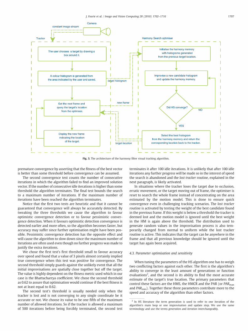
Fig. 3. The architecture of the harmony filter visual tracking algorithm.

2 In HS literature the term generation is used to refer to one iteration of thealgorithm's main loop or one improvisation and update step. We use the sameterminology and use the terms generation and iteration interchangeably.


premature convergence by asserting that the fitness of the best vectoris better than some threshold before convergence can be assumed.

The second convergence test counts the number of consecutiveiterations in which the algorithm failed to find an improved solutionvector. If the number of consecutive idle iterations is higher than somethreshold the algorithm terminates. The final test bounds the searchto a maximum number of iterations. If the maximum number ofiterations have been reached the algorithm terminates.

Notice that the first two tests are heuristic and that it cannot beguaranteed that convergence will always be accurately detected. Bytweaking the three thresholds we cause the algorithm to favouroptimistic convergence detection or to favour pessimistic conver-gence detection. When it favours optimistic detection convergence isdetected earlier and more often, so the algorithm becomes faster, butaccuracy may suffer since further optimisation might have been pos-sible. Pessimistic convergence detection has the opposite effect andwill cause the algorithm to slow down since the maximum number ofiterations are often used even though no further progress wasmade tojustify the extra iterations.

We chose the first test's first threshold small to favour accuracyover speed and found that a value of 3 pixels almost certainly impliedtrue convergence when this test was positive for convergence. Thesecond threshold simply guards against the unlikely event that all theinitial improvisations are spatially close together but off the target.The value is highly dependent on the fitness metric used which in ourcase is the Bhattacharrya coefficient. We chose the second thresholdas 0.62 to assure that optimisation would continue if the best fitness isnot at least equal to 0.62.

The second test's threshold is usually needed only when thetracker is lost and is not converging to any single coordinate be itaccurate or not. We choose its value to be one fifth of the maximumnumber of allowed iterations. So if the tracker is allowed a maximumof 500 iterations before being forcibly terminated, the second test

terminates it after 100 idle iterations. It is unlikely that after 100 idleiterations any further progress will be made so in the interest of speedthe search is abandoned and the lost tracker routine, explained in thenext paragraph, is likely activated.

In situations where the tracker loses the target due to occlusion,erratic movement, or the target moving out of frame, the optimiser isreset to search the whole frame instead of concentrating on the areaestimated by the motion model. This is done to ensure quickconvergence even in challenging tracking scenarios. The lost trackerroutine is activated by testing the weight of the best candidate foundin the previous frame. If this weight is below a threshold the tracker isdeemed lost and the motion model is ignored until the best weightin the HM is again above the threshold. The distribution used togenerate random values in the improvisation process is also tem-porarily changed from normal to uniform while the lost trackerroutine is active. This indicates that the target can be anywhere in theframe and that all previous knowledge should be ignored until thetarget has again been acquired.

4.3. Parameter optimisation and sensitivity

When tuning the parameters of the HS algorithm one has to weightwo conflicting factors against each other. The first is the algorithm'sability to converge in the least amount of generations or functionevaluations2, and the second is its ability to find the most accurateestimate of the target's true location. The primary parameters thatcontrol these factors are the HMS, the HMCR and the PAR (or PARmax

and PARmin). Together these three parameters contribute more to thespeed and accuracy of the algorithm than other factors.

image of Fig.�3

Fig. 5. A performance comparison using different values of the HMS.


The aim is to find the optimal value of these parameters that willgive us the most accurate estimate in the least amount of generations.We are also interested in the sensitivity to change of each of theseparameters. This will give us an indication of the robustness of thealgorithm and an indication of howmuch time has to be spent in fine-tuning the parameters.

We tested the algorithm's performance using several differentparameter values on a challenging tracking problem involving ahuman target walking along a footpath. A video was recorded using alow-cost web cam with a resolution of 352×288. The video quality islow and the target itself is only an 11×55 pixels area. As the targetmoves along the path it gets occluded by trees and other objects andalso moves through areas of increased light and shadow. Patterns inthe surrounding trees and reflections off the wet footpath also provideample local distractors that can cause the tracker to lose its target. Avideo frame from this example is shown in Fig. 4.

We start our analysis with the HMS and vary its value from 5 to 30.In all of the experiments the accuracy of the tracker was approxi-mately the same and no amount of optimisation saved the trackerfrom losing the target at certain points in the sequence. For this reasonit was decided to instead concentrate on speed. Fig. 5 shows a graphcomparing the speed of 25 different implementations correspondingto 25 different values of the HMS. The values in this graph weregathered by running the algorithm once for each frame in thesequence and calculating the average over all frames. This was donefor each value of HMS that we tested.

The algorithm is fairly stable to change in the HMS and even theworst choice of the HMS still resulted in an average of less than 200generations till convergence. The best choice for this example wasHMS=7 and experience showed that 6≤HMS≤8 almost always gavegood results. This agrees with the findings of Omran et al. that alsofound the optimal HMS to be between 2 and 10 [27].

Next the HMCR was investigated and varied from 0.5 to 0.99. Wefound the HMCR to be slightly more sensitive to change than the HMSbut still stable enough that any value between 0.7 and 0.99 couldsafely be chosen. However, the results show that higher values ofHCMR causes quicker convergence. This is likely due to the motionmodel accurately initialising the HM to be close to the correct locationwhich means that random search should be discouraged. A graphcomparing the performance of various values of the HMCR is shown inFig. 6. As shown, the lowest average number of generations tillconvergence was found at HMCR=0.95. This is the same value thatMahdavi et al. used in their examples [13].

Fig. 4. The challenging tracking problem used for parameter optimisation andsensitivity analysis.

The final parameter wewere interested inwas the pitch adjustmentrate. Since we use the improved harmony search (IHS) algorithm, thePAR is adjustedautomatically at the start of each generation.Weare thusinterested in the range of values the PAR is allowed to take and aim tofind the optimal values of the PARmin and the PARmax. PARmin was variedfrom 0.1 to 0.3 while PARmax was varied from 0.7 to 0.9. As claimed byMahdavi et al. [13], the effect of varying thePARmin and the PARmax is lessthan changing the PARdirectly and the algorithm therefore requires lessfine tuning. A contour plot comparing the average number ofgenerations till convergence for various values of PARmin and the PARmax

is shown in Fig. 7. The overall optimal values were found to bePARmax=0.9 and PARmin=0.3 but the performance difference betweenthese values and the values that did second best are almost negligible.

In this section we showed the effects of varying the HMS, HMCRand the PAR, particularly the effect it had on convergence speed.Varying the parameter values had little effect on the accuracy of thealgorithm in the example we used for testing. We rather focus onspeed and found the algorithm to give stable performance over a largerange of parameter values.

Optimal values were found for the HMS, HMCR and PAR pa-rameters. However, the optimisations aremade under the assumptionthat these parameters are not correlated and can be optimisedindependently. Relaxing this assumption would likely deliver moreoptimal values and further study into this is anticipated.

4.4. Computational complexity

The primary loop in the harmony search algorithm is the improvise-and-update loop that is repeated once every generation. Only one

Fig. 6. A performance comparison using different values of the HMCR.

image of Fig.�4

image of Fig.�5

image of Fig.�6

Fig. 7. A performance comparison using different values of the PAR.


evaluation of the fitness function is done in each generation so thetime spent optimising is almost fully dependent on the number ofgenerations till convergence. The number of generations needed forconvergence cannot easily be determined since it is dependent on thestate of the target and its surrounding environment at that time. Thisalsomeans that the time till convergencewill bedifferent for each frameand that the tracker's frame rate will not be constant.

An example of this inconsistent convergence speed is shown inFig. 8. It shows the number of generations needed for convergence atevery frame in the challenging tracking problem that was used in theprevious section. Notice that the tracker converges quickly at thebeginning of the sequence but later frequently only converges after500 generationswhichwas set to be themaximumnumber allowed inthis example. This is due to the target starting in an area where it isrelatively easy to track and then later moving away from the camerato an area where it is often occluded and where there are more localdistractors. Moving away from the camera also causes the target tobecome smaller which means a smaller histogram is created and lessdata is available from which to identify the target from. As the con-ditions for accurate tracking becomeworse the number of generationsneeded to converge increases.

It is therefore important that the criteria for convergence arechosen carefully so that number of generations till convergence iskept to a minimum. We previously mentioned that three tests areused to detect convergence and this example illustrates all three.When the target is easily identified, as was seen in the first fewframes, convergence is usually detected with the first test since all the

Fig. 8. The number of generations needed for convergence over all frames.

hypotheses in the HM quickly converge to the same optimal solution.This test frequently correctly detects convergence in less than 100generations as seen in Fig. 8. However, when tracking becomes moredifficult all the hypotheses will not converge to the same point and thefirst test will not be able to detect convergence. This is seen later in theexample when the target starts moving away from the camera. If thetarget is occluded or has moved out of frame the tracker will not findany good solution and the second test will eventually detect this stateand converge due to no progress being made for a prolonged numberof generations. This always leads to slower convergence since thealgorithm will only decide that no further progress can be madeafter numerous idle generations. As seen in the example this alwaystakes more than 100 generations and frequently takes more than 200generations.

However, when multiple local distractors are present it mayappear to the algorithm that is slowly making progress by convergingto multiple weaker hypotheses. This is the worst possible situationand it leads to the maximum number of generations reached beforeconvergence can be detected. We see this happening a few timesin the example of Fig. 8 when 500 generations are needed forconvergence.

It is clear that accurately detecting convergence is the key tominimising the computational complexity of the harmony filter algo-rithm. However, when the tracker is lost and cannot find any goodsolutions it is better to continue on with the next frame in the hopethat the situation improves rather than wastefully searching for asolution that does not exist.

Consider the example of Fig. 9. It illustrates the evolution of theHM by plotting theweight of the best hypothesis for every generation.First, notice that the initial best weight is less than 0.36 and the finalweight is less than 0.48. These lowweights indicate that the tracker isclearly lost and that even after 500 generations of searching the targetcould still not be found. The target is most likely occluded and the beststrategy would be to continue on to the next frame.

According to the graph the search should have been abandonedafter about 100 generations since no further progress to the besthypothesis was made. However, this is not as simple as it seems.Consider the more detailed view of the HM shown in Fig. 10. It showsthe location of both the best and worst hypothesis in the HM as pixelcoordinates. Notice that the minimum weight hypothesis changesfrequently and is still changing after 450 generations. This indicatesthat the HM was still being optimised even thought the final re-sult, the best hypothesis, reached its final value after less than 100generations.

Contrast this result with the example of Figs. 11 and 12. In this casethe HM is initialised with good hypotheses indicated by the high

Fig. 9. In this example the tracker is lost but continued to search until the maximumnumber of generations were reached.

image of Fig.�7

image of Fig.�8

image of Fig.�9

Fig. 10. A detailed view of the HM when convergence could not be detected. Fig. 12. A detailed view of the HM when convergence is correctly detected.


initial weight. After less than 100 generations the HM converges to asolution with a weight higher than 0.7 indicating that the target wasmost likely identified correctly. Notice also from Fig. 12 that the finallocation of the best and worst hypotheses are less than 5 pixels awayfrom each other indicating that it was the first convergence test thatcorrectly detected convergence here.

Deciding when to stop the search process and continue on to thenext frame is a trade-off between speed and accuracy. The algorithmwould benefit greatly from a better way of detecting occlusion andwhen there is no possibility of further improving the hypotheses inthe HM. The overall frame rate of the tracker could be significantlyimproved if better convergence tests were provided and further studyinto this is anticipated.

4.5. Theoretical advantages

Before moving on to results it is worth mentioning the theoreticaladvantages of the harmony filter. We start by investigating the wayprior information about the target motion is combined with the mostrecent observation of the target to accurately localize it. We comparethe way that the particle filter does this with the harmony filter'sapproach and argue that the harmony filter makes better use of allavailable information.

In most particle filters the motion model that forms the priorinformation is used as the proposal density function from which theinitial particle cloud is drawn. These particles are sampled from adensity function that does not take observational information fromthe most recent frame into account and is therefore frequently in-

Fig. 11. In this example all the hypotheses quickly converge to the same point andconvergence is correctly detected.

accurate. This inaccuracy is especially bad when fast erratic motioncauses the motion model to fail in accurately predicting the target'slocation. However, the particle filter does not ignore observationalinformation but uses it to score the particles by their probability ofhaving located the target. A resampling step is then performed thatfilters out low probability particles and duplicates high probabilityones.

Over several frames this process guides the particle cloud to themost likely location of the target. However, notice that the location ofthe particles in the search space have not changed since the initialsampling from the proposal distribution function. This means thatinaccuracies from the motion model can only be corrected, at best, inthe next frame following resampling.

In contrast, the harmony filter uses the most recent observationalinformation extensively and uses prior information only to initialisethe search process. As mentioned in previous sections, the harmonymemory is initialised by propagating the previous target locationthrough the motion model. This is similar to the way the particle filtergenerates the particle cloud by propagating the resampled cloud fromthe previous frame through the motion model. However, unlike theparticles of the particle filter, the improvisations in the harmony filterchange their position in the search space many times during theoptimisation process by comparing with current observationalinformation. In this way inaccuracies in prior information from themotion model can be immediately corrected and the error does notpropagate to the next frame. Notice though, that when the priorinformation is accurate the harmony filter makes full of this bydetecting early convergence and saving computational resources byterminating the search process. In contrast the particle filter alwaysevaluates all particles in every frame even when an earlier evaluatedparticle successfully located the target.

By effectively using prior information when it is accurate anddiscarding it when it is not, the harmony filter potentially gains atheoretical advantage over the particle filter that always relies onprior information to generate the particle cloud. The harmony filterrelies heavily on the most current observational information toimprove the initial improvisations in contrast with the particle filterthat only uses it to score particles without changing their initialposition in the search space.

5. Results

In this section we demonstrate the harmony filter's ability to trackobjects in various challenging environments. The algorithm is alsocompared with various other successful tracking algorithms includingthe unscented Kalman filter (UKF) and the particle filter. We con-centrate on three video sequences that test the tracker's ability to

image of Fig.�10

image of Fig.�11

image of Fig.�12

Fig. 14. An accuracy comparison between different tracker implementations forexample 1.


accurately track a target through quick erratic motion, local dis-tractors, occlusion, low resolution images, bad and variable lightingand the target moving in and out of frame.

In all three examples we use the parameter values found by thesensitivity analysis of Section 4.3. BWmin and BWmax were chosen as 1and 12 respectively to favour accuracy over speed. The thresholdvalues for the convergence test were chosen as detailed in Section 4.2.To ensure a fair comparison none of these values were modified orfine tuned to specifically improve performance in any of the threeexperiments but was kept at the values stated here. In order to ensurethat our comparison with the UKF and particle filter implementationsare fair we use the exact same motion model discussed in Section 4.2,as the dynamic model used in updating the particle filter and the UKF.

Our first two examples were captured with a low cost web cam at aresolution of 352×288 at 15 frames/s. The first example is the sameone used for the parameter sensitivity analysis of the previous sectionand thus includes all the tracking challenges associated withocclusion, poor quality images, changing light and local distractors.In order to test tracker accuracy we manually labelled the video byidentifying the centre of the tracked object in each frame. The distancebetween the true centre and the centre estimated by the tracker isthen calculated and used as an accuracy metric. This only gives anindication of the true accuracy though since scale changes or changesin the size of the tracked object are ignored. Figs. 13 and 14 show thespeed and accuracy of the harmony filter comparedwith two differentimplementations of a particle filter based tracker (one using 300particles and one using 500) and an unscented Kalman filter basedtracker.

In order to keep the details of the graph large enough to dis-tinguish individual traces, only the first portion of the graph is shownin Fig. 14. Notice that the two particle filter implementations con-stantly lose the target while the UKF and harmony filter implementa-tions usually stay within 50 pixels of the target's centroid. This is likelydue to local distractors pulling the particle clouds of the particle filtersaway from the target and the fairly predictable motion of the targetcausing the UKF to accurately predict the target's next position. Theharmony filter proved robust in the vicinity of local distractors andcould also quickly re-acquire the target after occlusion. This issomething the UKF had trouble with but was better performed bythe particle filters. Due to the harmony filter detecting convergencesooner or later depending on the environment, its speed variessignificantly compared with other implementations as seen in Fig. 13.However, on average the harmony filter was faster than both theparticle filters and the UKF. The average time till convergence for allthree algorithms is shown in Table 1.

Two examples that illustrate the difference in accuracy betweenimplementations are shown in Fig. 15. For each example three screen

Fig. 13. A speed comparison between different tracker implementations for example 1.

captures are shown that correspond to the harmony filter, a particlefilter implementation and a UKF implementation. In each image theestimated position of the target is shown by a red square.

In the second example an orange square is tracked on a back-ground with few local distractors. This environment makes it mucheasier for the tracker to recognise the target and one would expect theperformance of all the trackers to improve compared to the previousexample. However, this example was used to test the tracker'sperformance during quick erratic movement that is difficult to predictusing the simple motion model used. This motion was generated byrapidly rotating and translating the camera in random directions. Thecamera's lens was also occluded for prolonged periods of time to testthe tracker's recovery of the target after it has been lost for manyframes.

The results from the performance comparison of the secondsequence is seen in Figs. 16 and 17. In the speed comparison graph wesee a situation similar to the one in the first example. While theparticle filters and the UKF show fairly constant performance, theharmony filter's performance varies depending on the environment atthat frame. Due to the prolonged periods of occlusion, during whichthe harmony filter took a long time to converge, its speed is morecomparable to the other trackers but is still slightly faster on average.Table 2 shows the average time till convergence for this example.

However, when comparing accuracies the harmony filter proves tobe the most robust implementation. As soon as the erratic motionstarted the UKF lost track of the target and never got the opportunityto recover properly. The particle filters also lost track but sometimesrecovered after only a few frames. The harmony filter recoveredalmost immediately from erratic motion and prolonged occlusion, andwas still robustly tracking the target at a time when all other trackerswere still trying to recover.

Two examples illustrating this claim are shown in Fig. 18. As beforethree images are shown for each example, one for every filterimplementation. In the first example the camera lens is covered by ahand for several frames and then removed. The harmony filterrecovered after the hand was removed and immediately found thetarget again. However, the particle filter and the UKF could not

Table 1Average time till convergence for example 1.

Algorithm Time till convergence (ms)

Harmony filter 20.44Particle filter (300 particles) 45.73Particle filter (500 particles) 72.48UKF 24.22

image of Fig.�13

image of Fig.�14

Fig. 15. Illustrated here are two challenging tracking scenarios from the first example sequence. In the first scenario (the first column of this figure) local distractors in the reflectivepavement and changing light conditions cause the particle filter to get lost. The UKF and harmony filter proved to be more robust. In the second scenario the target is partiallyoccluded causing the particle filter to again lose the target. Both the UKF and harmony filter managed to stay with the target but the harmony filter was better aligned with the trueposition of the target.


recover from this situation. A similar situation is seen in the secondexample. Quick erratic motion causes the UKF and particle filter tolose the target without recovering but the harmony filter managed toonly lose the target momentarily and quickly recovered.

Our final example comes from a sequence recorded for the CAVIARproject [28]. It was chosen to test the tracker's ability to accurately tracka target that changes its basic shape constantly. The sequence shows twomen fighting each other and ends with one man knocking the other to

the floor and running away. Themen often occlude each other or part ofeach other, and by ducking, waving their arms and falling to the floorthey change their shape as well. Notice also that the rectangle used toidentify and model the target is now a very poor fit to the shape of thetarget. This makes it difficult for trackers to maintain the target positionthrough local distractors in the scene and only themost robust oneswillsucceed. For these reasons it is challenging to track one of themen usinga system that models targets as histograms of rectangular patches.

image of Fig.�15

Fig. 16. An accuracy comparison between different tracker implementations for example 2. The sub-image is an enlarged section of the graph illustrating and comparingperformance immediately following a long period of occlusion. The Harmony Filter is shown to recover quickly from occlusion while the UKF and particle filters only momentarilyrecover the target for one or two frames.


Two tracking examples from this sequence are shown in Fig. 19.The aim is to track the man wearing black and in the first example theman wearing the light blue shirt partially occluded the other man bymoving in front of him. This action caused both the particle filter andthe UKF to lose the target while the harmony filter managed torobustly track it. In the second example the man in black is knocked tothe ground causing the model of the target to change considerably.This made all three trackers much more sensitive to local distractorsin the image and only the harmony filter managed to stay with theoriginal target.

Speed and accuracy comparisons from this example are shown inFigs. 20 and 21. The speed comparison was similar to the previousexamples with the harmony filter again the fastest on average. Theaverage times till convergence are shown in Table 3. It also proved tobe the most accurate even though it lost the target near the end of thesequence without successfully recovering.

5.1. Discussion

In this section we used three example tracking problems toevaluate the harmony filter's ability to robustly and efficiently track


an arbitrary target through a video sequence. Speed and accuracymetrics were used to compare its performance with other popularalgorithms used in visual tracking. The same target model and motionmodel was used in all tracker implementations. In all three examplesthe harmony filter proved to be consistently more accurate than theother algorithms and was also faster on average.

However, one problem with the harmony filter is that its speed isdependent on the tracking environment and thus cannot guarantee aconstant frame rate. As seen in the speed comparisons of Figs. 13, 17and 21, the harmony filter is not consistently the fastest over allframes. While the speed of the particle filter and UKF remains con-sistent, we see spikes in the harmony filter's trace that indicate slowerthan usual convergence. If we compare the location of these spikeswith the corresponding locations in Figs. 14, 16 and 20, we see thatslow convergence is usually accompanied by bad accuracy from allimplementations. As previously illustrated, the frames with pooraccuracy are most often the result of occlusion. During occlusion theharmony filter cannot find a good solution in the frame and localdistractors that resemble the target can cause it to take a long timebefore the search is abandoned. The same situation can also occurduring erratic motion when the target is usually blurred or deformed,or when the target is rotated as in our third example.

Constant performance is especially important in real-time applica-tions since the available time till convergence is bounded. Usually theharmony filter returned the estimated location of the target longbefore the other algorithms but in some cases it took the longest.

By limiting the maximum number of allowable generations thatHarmony Search can use, the maximum time till convergence can becapped and thus guarantee that the frame ratewill never drop below acertain level. The frame rate still won't be constant since earlyconvergence can still occur but it will be bounded above. However,




image of Fig.�16

image of Fig.�17

Fig. 18. Two challenging tracking scenarios are shown from the second example. In the first example the target is occluded for several frames and recovery from occlusion iscompared between the various trackers. In the second example the camera is pulled and rotated to simulate quick and erratic motion of the target. Only the harmony filter couldsuccessfully track the target in both situations.


capping the number of generations too low runs the risk of producinginaccurate estimations. As long as the filter's speed is bounded to beno slower than a chosen limit, a non-constant speed is acceptableeven in real-time applications.

6. Conclusion

Algorithms for efficient and accurate visual tracking have been thesubject of much computer vision research over the years. The most

successful of these have all been based on statistical filters or MonteCarlo methods, for example, the Kalman filter and the particle filter.However, these algorithms often suffer in accuracy when the target'smotion cannot be accurately modelled or when the sensor or motionnoise cannot be assumed to be Gaussian.

The harmony search algorithm is able to find an optimal solutionvector in a large multi-dimensional space without making any as-sumptions on the system noise or the shape of the search area. Thismakes it a potentially good algorithm for finding the best estimate of

image of Fig.�18

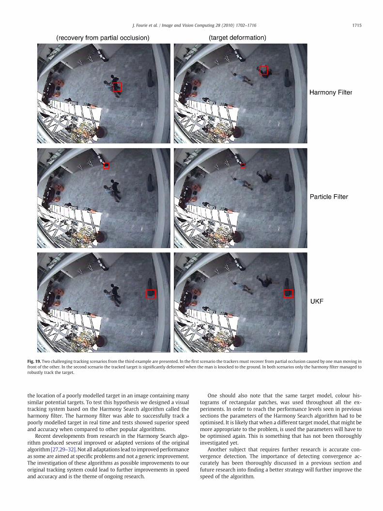
Fig. 19. Two challenging tracking scenarios from the third example are presented. In the first scenario the trackers must recover from partial occlusion caused by one manmoving infront of the other. In the second scenario the tracked target is significantly deformed when the man is knocked to the ground. In both scenarios only the harmony filter managed torobustly track the target.


the location of a poorly modelled target in an image containing manysimilar potential targets. To test this hypothesis we designed a visualtracking system based on the Harmony Search algorithm called theharmony filter. The harmony filter was able to successfully track apoorly modelled target in real time and tests showed superior speedand accuracy when compared to other popular algorithms.

Recent developments from research in the Harmony Search algo-rithm produced several improved or adapted versions of the originalalgorithm[27,29–32]. Not all adaptations lead to improvedperformanceas some are aimed at specific problems and not a generic improvement.The investigation of these algorithms as possible improvements to ouroriginal tracking system could lead to further improvements in speedand accuracy and is the theme of ongoing research.

One should also note that the same target model, colour his-tograms of rectangular patches, was used throughout all the ex-periments. In order to reach the performance levels seen in previoussections the parameters of the Harmony Search algorithm had to beoptimised. It is likely that when a different target model, that might bemore appropriate to the problem, is used the parameters will have tobe optimised again. This is something that has not been thoroughlyinvestigated yet.

Another subject that requires further research is accurate con-vergence detection. The importance of detecting convergence ac-curately has been thoroughly discussed in a previous section andfuture research into finding a better strategy will further improve thespeed of the algorithm.

image of Fig.�19

Fig. 20. An accuracy comparison between different tracker implementations forexample 3.



The current version of the harmony filter outperformed both theparticle filter implementation and the UKF implementation in all ofour experiments. To the author's knowledge this is the first time thatthe Harmony Search algorithm has been adapted for use in a visualtracking system and our initial results showed it to be a superioralternative to the popular particle and Kalman filter approaches.

References

[1] V. Ferrari, T. Tuytelaars, L.V. Gool, Real-time Affine Region Tracking And CoplanarGrouping, Conference on Computer Vision and Pattern recognition 2, 2001, p. 226.

[2] A.D. Bue, D. Comaniciu, V. Ramesh, C.S. Regazzoni, Smart Cameras With Real-timeVideo Object Generation, ICIP, 2002, pp. 429–432.

[3] U. Handmann, T. Kalinke, C. Tzomakas, M. Werner, W. von Seelen, An imageprocessing system for driver assistance, Image and Vision Computing 18 (5)(2000) 367–376.

[4] P. Gutman, M. Velger, Tracking targets using adaptive Kalman filtering, IEEETransactions on Aerospace and Electronic Systems 26 (1990) 691–699.




[5] M. Li, B. Hong, Z. Cai, R. Luo, Novel Rao-Blackwellized particle filter for mobilerobot SLAM using monocular vision, International Journal of IntelligentTechnology 1 (1) (2006) 63–69.

[6] M. Isard, A. Blake, Condensation–conditional density propagation for visualtracking, IJCV 29 (1) (1998) 5–28.

[7] M. Minami, J. Agbanhan, T. Asakura, Manipulator visual servoing and tracking offish using a genetic algorithm, Industrial Robot: An International Journal 26 (4)(1999) 278–289.

[8] Y. Morsly, M.S. Djouadi, Genetic Algorithm combined to IMM approach forTracking Highly Maneuvering Targets, IAENG International Journal of ComputerScience (2008) 35 advanced online publication 19 February 2008.

[9] I.A. Sulistijono, N. Kubota, Human head tracking based on particle swarmoptimization and genetic algorithm, Journal of Advanced ComputationalIntelligence and Intelligent Informatics 11 (6) (2007) 681–687.

[10] X. Zhang, S. Maybank,W. Hu, X. Li, M. Zhu, Sequential particle swarm optimisationfor visual tracking, Proceedings of CVPR, 2008, pp. 1–8.

[11] Z.W. Geem, J.H. Kim, G. Loganathan, A new heuristic optimization algorithm:harmony search, Simulation 76 (2) (2001) 60–68.

[12] K.S. Lee, Z.W. Geem, A new meta-heuristic algorithm for continuous engineeringoptimization: harmony search theory and practice, Computer Methods in AppliedMechanics and Engineering 194 (2005) 3902–3933.

[13] M. Mahdavi, M. Fesanghary, E. Damangir, An improved harmony search algorithmfor solving optimization problems, Applied Mathematics and Computation 188(2007) 1567–1579.

[14] O. Alia, R. Mandava, D. Ramachandram, M. Aziz, Dynamic fuzzy clustering usingharmony search with application to image segmentation, Signal Processing andInformation Technology (ISSPIT), 2009 IEEE International Symposium on, , 2009,pp. 538–543, doi:10.1109/ISSPIT.2009.5407590.

[15] J. Fourie, S. Mills, R. Green, Visual Tracking Using the Harmony Search Algorithm,Image and Vision Computing New Zealand, IVCNZ 23rd International Conference, ,2008, pp. 1–6, doi:10.1109/IVCNZ.2008.4762068.

[16] J. Fourie, S. Mills, R. Green, Directed Correspondence Search: Finding FeatureCorrespondences in Images Using the Harmony Search Algorithm, Image andVision Computing New Zealand (IVCNZ), 2009.

[17] Z. Geem, K. Lee, Y. Park, Application of harmony search to vehicle routing,American Journal of Applied Sciences 2 (12) (2005) 1552–1557.

[18] Z.W. Geem, et al., Recent Advances In Harmony Search Algorithm, 1st Edition, Vol.270 of Studies in Computational Intelligence, Springer, Berlin, 2010.

[19] P. Li, T. Zhang, B. Ma, Unscented Kalman filter for visual curve tracking, Image andVision Computing 22 (2004) 157–164.

[20] K. Nummiaro, E. Koller-Meier, L.V. Gool, An adaptive color-based particle filter,Image and Vision Computing 21 (1) (2003) 99–110, doi:10.1016/S0262-8856(02)00129-4.

[21] T. Chen, R. Luo, T. Hsiao, Visual tracking using adaptive color histogrammodel, The25th Annual Conference of the IEEE Industrial Electronics Society, Vol. 3, 1999,pp. 1336–1341.

[22] M. Swain, D. Ballard, Indexing Via Color Histograms, Proceedings of The ThirdInternational Conference on Computer Vision, 1990, pp. 390–396.

[23] D. Comaniciu, V. Ramesh, P. Meer, Kernel-based object tracking, IEEE Transactionson Pattern Analysis and Machine Intelligence 25 (5) (2003) 564–575 doi:http://dx.doi.org/10.1109/TPAMI.2003.1195991.

[24] T. Kailath, The divergence and Bhattacharyya distance measures in signalselection, IEEE Transactions on Communication Technology 15 (1) (1967) 52–60.

[25] H. Guyen, G. Kogut, R. Barua, A. Burmeister, N. Pezeshkian, D. Powell, N.Farrington, M. Wimmer, B. Cicchetto, C. Heng, V. Ramirez, A Segway RMP-BasedRobotic Transport System, SPIE Proc. 5609: Mobile Robots XVII, 2004.

[26] J. Sattar, A Visual Servoing System for an Amphibious Legged Robot, Master'sthesis, McGill University, Montréal, Québec (2005).

[27] M. Omran, M. Mahdavi, Global-best harmony search, Applied Mathematics andComputation 198 (2008) 643–656.

[28] EC funded CAVIAR project/ist 2001 37540, http://homepages.inf.ed.ac.uk/rbf/CAVIAR/ (July 2008).

[29] M. Fesanghary, M. Mahdavi, M. Minary-Jolandan, Y. Alizadeh, Hybridizingharmony search algorithm with sequential quadratic programming for engineer-ing optimization problems, Computer Methods in Applied Mechanics andEngineering 197 (33-40) (2008) 3080–3091.

[30] L. Hong-qi, L. Li, T. Kim, X. Shao-long, An improved PSO-based of harmony searchfor complicated optimization problems, International Journal of Hybrid Informa-tion Technology vol 1 (No. 1) (2008) 57–64.

[31] Z.W. Geem, Improved harmony search from ensemble of music players, LectureNotes in Computer Science 4251 (2006) 86–93.

[32] Z.W. Geem, Particle-swarm harmony search for water network design, Engineer-ing Optimization 41 (4) (2009) 297–311.

http://dx.doi.org/10.1109/ISSPIT.2009.5407590

http://dx.doi.org/10.1109/IVCNZ.2008.4762068

http://dx.doi.org/10.1109/TPAMI.2003.1195991

http://dx.doi.org/10.1109/TPAMI.2003.1195991

http://homepages.inf.ed.ac.uk/rbf/CAVIAR/

http://homepages.inf.ed.ac.uk/rbf/CAVIAR/

image of Fig.�20

image of Fig.�21

harmony filter: a robust visual tracking system using the improved harmony search algorithm

Documents