handbook to the partners in flight population estimates...

Handbook to the Partners in Flight Population Estimates Database, Version 2.0

Partners in Flight Science Committee

January 2013 Authors: Peter J. Blancher, Environment Canada Kenneth V. Rosenberg, Cornell Lab of Ornithology Arvind O. Panjabi, Rocky Mountain Bird Observatory Bob Altman, American Bird Conservancy Andrew R. Couturier, Bird Studies Canada Wayne E. Thogmartin, United States Geological Survey

Recommended citation: Blancher, PJ, KV Rosenberg, AO Panjabi, B Altman, AR Couturier, WE Thogmartin and the Partners in Flight Science Committee. 2013. Handbook to the Partners in Flight Population Estimates Database, Version 2.0. PIF Technical Series No 6. http://www.partnersinflight.org/pubs/ts/

http://www.partnersinflight.org/pubs/ts/

2

Preface:

This Handbook outlines updates and other changes made to the Partners in Flight (PIF) Population Estimates Database since 2007; it is current to Version 2.0 of the PIF Population Estimates Database (http://www.rmbo.org/pif_db/laped/). These changes do not alter the general approach outlined in the original Guide to the PIF Population Estimates (Blancher et al. 2007, http://www.rmbo.org/pif_db/laped/guide.aspx), which should be consulted for a full description of methods, potential uses of data and their limitations, and the meaning of individual variables, keeping in mind the changes described here. Version 2.0 of the database is a companion to PIF’s “Saving Our Shared Birds” document (Berlanga et al. 2010, http://www.savingoursharedbirds.org/), and as such, most estimates included in the database were produced in 2008 for use in that report. Though Saving Our Shared Birds did not report species-specific population estimates (as was done in Rich et al. 2004), updated estimates were relied on for scoring the Population Size assessment factor, for estimating the magnitude of loss of common birds in steep decline, and to illustrate the high percentage of birds shared internationally. This update addresses some of the recommendations of the Thogmartin et al. (2006) peer review, however much work remains to fully address the limitations outlined by Thogmartin et al. (2006), Blancher et al. (2007), Confer et al. (2008), Thogmartin (2010) and Matsuoka et al. (2012).

Summary of Changes:

We made the following updates and revisions (see next section for details):

Updated Breeding Bird Survey (BBS) count data to 1998-2007 (formerly 1990-1999);

Used Ontario atlas point count data from 2001-2005 to fill a large gap in BBS coverage in northern Ontario and adjacent provinces;

Updated population estimates from species-specific surveys where possible;

Changed some Detection Distances to improve comparisons across species, based on detection data in a few other large datasets (from Ontario, California, Colorado, and boreal Canada);

Used species-specific Pair Adjustments, rather than a multiple of 2 for all species;

Revised Time of Day Adjustments to include BBS data to 2005 (previously to 2002);

Used NatureServe digital range data to extrapolate populations south of the U.S. (formerly estimated by PIF Science Committee members);

Reduced estimates for regions in the Canadian arctic by the proportion of permanent ice cover in those regions;

Where data from one region were extrapolated into a neighbouring region to fill a data gap (mainly in boreal and arctic Canada), we adjusted extrapolated values based on the relative extent of species breeding range in the two regions;

Modified the presentation of data to add estimates by country and include all landbirds with BBS data;

http://www.rmbo.org/pif_db/laped/

http://www.rmbo.org/pif_db/laped/guide.aspx

http://www.savingoursharedbirds.org/

3

Added a calculator that allows users to modify underlying parameters and see their effect on the population estimate.

Thus these new estimates are a result of numerous changes both in the data included and in the process. So users should use caution when comparing an estimate from the original database (Version 2004) to one from version 2.0.

Contents: Preface 2

Summary of Changes 2 Details of Changes Made since original estimates (Version 2004) 4

o Data updates o Analytical changes o Changes to presentation

Results – Summary of changes in the estimates 8

Next Steps 10 Acknowledgements 12 Literature Cited 13 Appendix 1: Updated Example of Population Estimates 15 Appendix 2: Example Use of the Population Estimate Calculator 16

4

Details of Changes Made since original estimates (Version 2004):

o Data Updates:

Breeding Bird Survey (BBS) data

The original version (2004) of the PIF Population Estimates Database relied on BBS count data

from 1990-1999, stratified by geo-political regions in U.S. and Canada, as a basis for the

estimating average density of birds. Analyses for the 2010 Saving Our Shared Birds document

used BBS count data from 1998-2007, so that estimates are in effect eight years more current,

important mainly for populations undergoing rapid increases or declines, or in regions where

sampling effort has increased.

We updated Time of Day Adjustments to make use of stop by stop BBS count data from 1997 to

2005, versus 1997-2002 in the original database. The additional years of data increased

samples sizes and thus our ability to estimate a more precise adjustment factor.

Ontario Breeding Bird Atlas point count data

The BBS does not sample the Hudson Bay Lowlands in northern Ontario or neighbouring

provinces, due to a dearth of roads and people. These lowlands encompass a large portion

(346,000 km2) of the Taiga Shield and Hudson Plains Bird Conservation Region (BCR 7; U.S.

NABCI Committee 2000). In the original version of the PIF database, population estimates for

this region were extrapolated from relatively few BBS routes scattered across the vast Taiga

Shield portion of BCR 7. In this update, we replaced extrapolations with estimates based on

atlas point count data collected in Ontario during 2001-2005 (Cadman et al. 2007).

Point count averages were calculated for each species in each of 82 10 x 10 km2 atlas squares in

Ontario BCR 7 that included at least 10 point counts – 1,855 point counts in all, each of 5

minutes duration. A point count average for the full region was calculated by averaging the

square averages, stratifying by the extent of species breeding range in each of 3 ecoregions

(Hudson Bay Coast, Northern Taiga, James Bay) within BCR 7. These region-wide count

averages were then converted to a BBS route average equivalent, based on a comparison of

atlas point count averages and BBS route averages in BCR 12 Ontario, a region well sampled by

both programs in 2001-2005.

BBS equivalent averages for Ontario BCR 7 were also used to fill gaps in Manitoba and Quebec

portions of BCR 7, averaged with BBS data from Labrador BCR 7 in the case of Quebec, and

adjusted by the relative extent of species breeding range in Ontario versus the other regions.

5

Species-specific updates

Several range-wide population estimates in the PIF database are based on species-specific

surveys and knowledge, especially for listed Endangered Species. Where updates were

available, we updated these (see source information in database); in many cases, estimates

remained unchanged after review.

o Analytical Changes:

Detection Distances

Detection Distance categories are used to convert BBS counts into rough estimates of density,

with distance of detection differing widely among species. We reviewed and, in many cases,

modified distance categories used for each species, based on information received following a

PIF request for input, new published data (e.g., Hamel et al. 2009), and comparisons with

distance information in four regional point count datasets (California, Colorado, Ontario, boreal

Canada). The main intent was to improve relative Detection Distances assignments among

species, and thus increase reliability of PIF’s Population Size assessment scores (PS score).

Three distance categories were added (50m, 100m, 300m) to provide smaller jumps between

categories, and to increase correlation of distances assigned versus those in comparison

datasets.

After these modifications were made, correlations with distance information in regional

datasets improved to about 0.7 or greater, similar to correlations among regional datasets

where the same or similar species were included. No attempt was made to adjust all species to

average (usually shorter) distances in the regional datasets, in part because regional datasets

employed different count methods, included off-road counts, and did not account for

movement by birds during counts. Nevertheless, PIF’s population estimates appear to be

generally conservative relative to other sources of estimates (Rosenberg and Blancher 2005,

Matsuoka et al. 2012), most likely as a result of the use of relatively long Detection Distances.

Pair Adjustments

Original estimates included a multiple of 2 for all species on the assumption that, on average

across BBS routes at the peak time of detection, no more than one bird per pair is detected on

BBS counts. However, we know that detection of both members of a pair differs across species,

largely depending on how they are detected on BBS routes (e.g., by song or by sight, singly vs.

in groups). To improve the relativity of estimates across species, we assigned species to one of

five Pair Adjustment categories (1.0, 1.25, 1.5, 1.75, 2.0) after consideration of the following

information for each species:

6

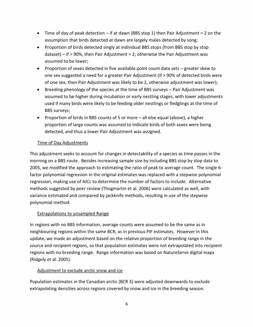
Time of day of peak detection – if at dawn (BBS stop 1) then Pair Adjustment = 2 on the

assumption that birds detected at dawn are largely males detected by song;

Proportion of birds detected singly at individual BBS stops (from BBS stop by stop

dataset) – if > 90%, then Pair Adjustment = 2; otherwise the Pair Adjustment was

assumed to be lower;

Proportion of sexes detected in five available point count data sets – greater skew to

one sex suggested a need for a greater Pair Adjustment (if > 90% of detected birds were

of one sex, then Pair Adjustment was likely to be 2, otherwise adjustment was lower);

Breeding phenology of the species at the time of BBS surveys – Pair Adjustment was

assumed to be higher during incubation or early nestling stages, with lower adjustments

used if many birds were likely to be feeding older nestlings or fledglings at the time of

BBS surveys;

Proportion of birds in BBS counts of 5 or more – all else equal (above), a higher

proportion of large counts was assumed to indicate birds of both sexes were being

detected, and thus a lower Pair Adjustment was assigned.

Time of Day Adjustments

This adjustment seeks to account for changes in detectability of a species as time passes in the

morning on a BBS route. Besides increasing sample size by including BBS stop by stop data to

2005, we modified the approach to estimating the ratio of peak to average count. The single 6-

factor polynomial regression in the original estimates was replaced with a stepwise polynomial

regression, making use of AICc to determine the number of factors to include. Alternative

methods suggested by peer review (Thogmartin et al. 2006) were calculated as well, with

variance estimated and compared by jackknife methods, resulting in use of the stepwise

polynomial method.

Extrapolations to unsampled Range

In regions with no BBS information, average counts were assumed to be the same as in

neighbouring regions within the same BCR, as in previous PIF estimates. However in this

update, we made an adjustment based on the relative proportion of breeding range in the

source and recipient regions, so that population estimates were not extrapolated into recipient

regions with no breeding range. Range information was based on NatureServe digital maps

(Ridgely et al. 2005).

Adjustment to exclude arctic snow and ice

Population estimates in the Canadian arctic (BCR 3) were adjusted downwards to exclude

extrapolating densities across regions covered by snow and ice in the breeding season.

7

Advanced very high resolution radiometer (AVHRR) land cover data from 1995 (Natural

Resources Canada 1995) provided the basis for estimating % cover of snow and ice in the three

ecozones that comprise BCR 3: Arctic Cordillera (75.3% snow and ice), Northern Arctic (29.0%),

and Southern Arctic (1.7%). Bird species abundances were adjusted according to the

proportion of the population estimate from each of the three ecozones.

o Changes to Presentation of Data

The database structure remains largely the same as in the previous version, with separate

downloadable spreadsheets available for BCR-wide estimates, state- province- and territory-

wide estimates, building block estimates at the intersection of these two (BCR x jurisdiction

geopolitical polygons), as well as estimates at the continental scale. As before, the latter

spreadsheet includes BBS-wide and global estimates by species in addition to estimates for the

U.S. and Canada combined. New in this updated spreadsheet are estimates for each country

individually. Other changes in content include:

Additional species entries - the regional spreadsheets now include entries for all

landbirds with BBS data, even when range-wide species estimates were from other

sources; in the latter case, underlying data are presented but no BBS-based population

estimate is calculated.

BBS Population Calculator - each downloadable spreadsheet now includes a “BBS Pop’n

Calculator” column, which uses the underlying data in the table to calculate a BBS-based

population estimate. Subject to differences in rounding, this value should be identical

to the values in the “Population Estimate” and “Population Estimate (unrounded)”

columns; in the continental spreadsheet the calculator value will be the same as the

value in the “Population Estimate BBS” and “BBS Pop’n Estimate (unrounded)” columns.

Users can now make changes to any of the underlying data (BBS average, Detection

Distance, Pair Adjustment, Time of Day Adjustment) and/or include an adjustment for

biased coverage of the landscape by BBS (Landscape Bias Adjustment), and instantly see

the revised estimate in the Calculator column. Examples are provided below in

Appendix 2.

8

Results: Changes to the Estimates

Sources for global population estimates in the updated database are generally split into two

groups:

338 species with calculated estimates, based on a combination of BBS counts, Ontario

Atlas point counts, checklist data combined with Breeding Bird Census densities for the

Northwest Territories & Nunavut, and range extrapolations.

118 species with other (non-calculated) sources of population estimates. Though not

relied on for estimates, BBS count data are available (and included in the database) for

most (93) of these species.

Of the non-calculated global estimates, 30 were modified in this update, resulting in 11 changes

to PIF’s Population Size (PS) assessment scores, 8 based on higher estimates, 3 lower.

We updated all of the calculated estimates. The following comparisons, including results shown

in Figures 1-3 and Table 1, are from 319 species detected on at least 20 BBS routes in both

decades.

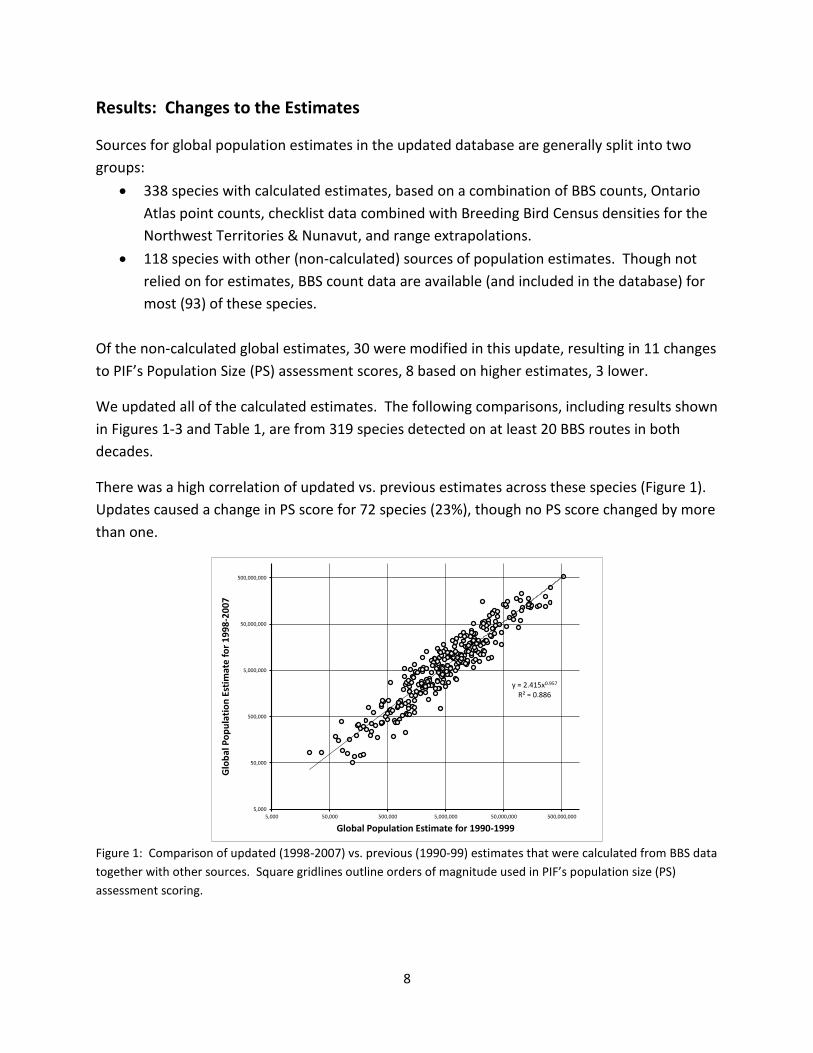
There was a high correlation of updated vs. previous estimates across these species (Figure 1).

Updates caused a change in PS score for 72 species (23%), though no PS score changed by more

than one.

y = 2.415x0.957

R² = 0.886

5,000

50,000

500,000

5,000,000

50,000,000

500,000,000

5,000 50,000 500,000 5,000,000 50,000,000 500,000,000

Glo

bal

Po

pu

lati

on

Est

imat

e f

or

19

98

-20

07

Global Population Estimate for 1990-1999

Figure 1: Comparison of updated (1998-2007) vs. previous (1990-99) estimates that were calculated from BBS data

together with other sources. Square gridlines outline orders of magnitude used in PIF’s population size (PS)

assessment scoring.

9

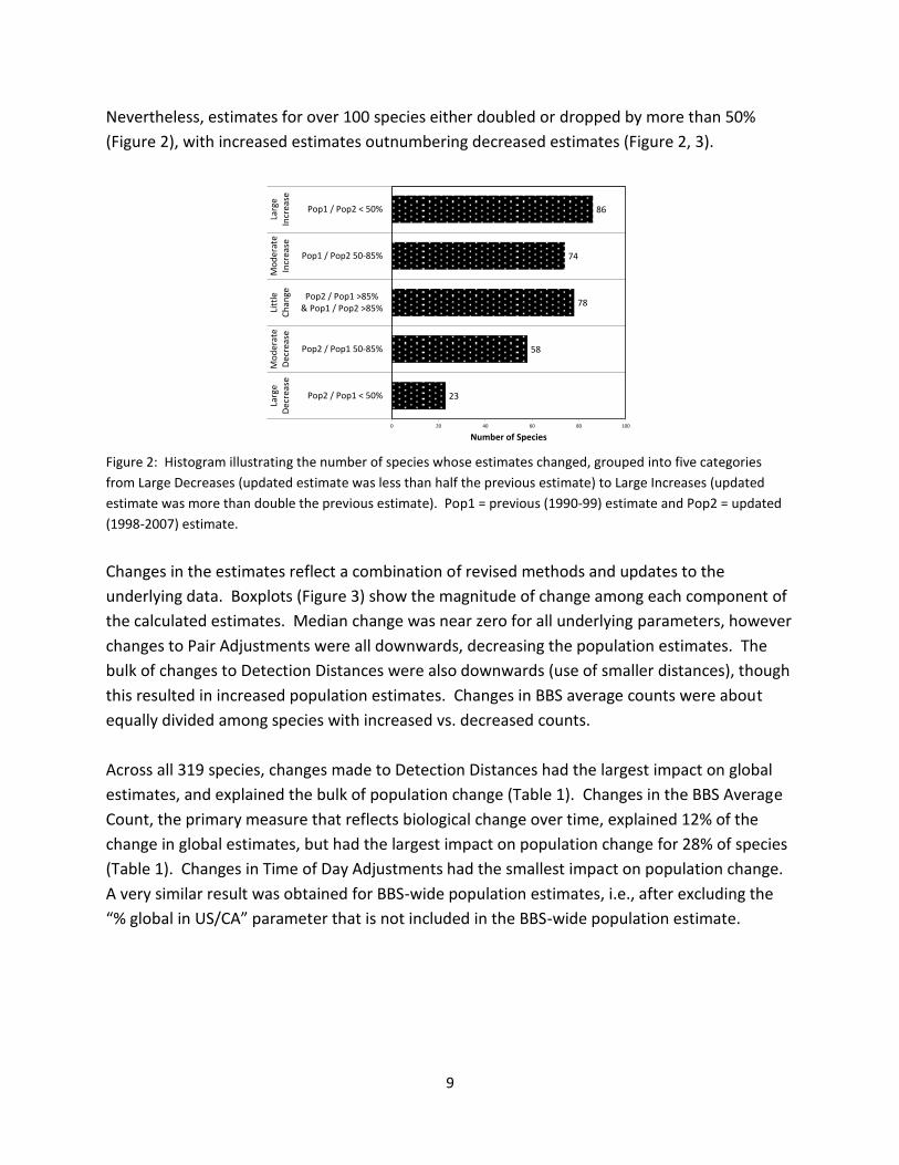
Nevertheless, estimates for over 100 species either doubled or dropped by more than 50%

(Figure 2), with increased estimates outnumbering decreased estimates (Figure 2, 3).

23

58

78

74

86

0 20 40 60 80 100

Pop2 / Pop1 < 50%

Pop2 / Pop1 50-85%

Pop2 / Pop1 >85%& Pop1 / Pop2 >85%

Pop1 / Pop2 50-85%

Pop1 / Pop2 < 50%

Larg

eD

ecre

ase

Mo

der

ate

Dec

reas

eLi

ttle

Ch

ange

Mo

der

ate

Incr

ease

Larg

eIn

crea

se

Number of Species

Figure 2: Histogram illustrating the number of species whose estimates changed, grouped into five categories

from Large Decreases (updated estimate was less than half the previous estimate) to Large Increases (updated

estimate was more than double the previous estimate). Pop1 = previous (1990-99) estimate and Pop2 = updated

(1998-2007) estimate.

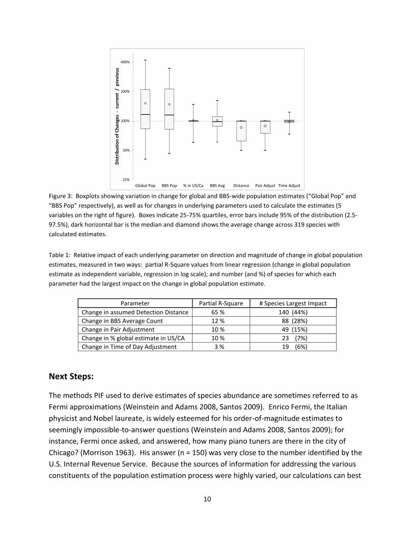
Changes in the estimates reflect a combination of revised methods and updates to the

underlying data. Boxplots (Figure 3) show the magnitude of change among each component of

the calculated estimates. Median change was near zero for all underlying parameters, however

changes to Pair Adjustments were all downwards, decreasing the population estimates. The

bulk of changes to Detection Distances were also downwards (use of smaller distances), though

this resulted in increased population estimates. Changes in BBS average counts were about

equally divided among species with increased vs. decreased counts.

Across all 319 species, changes made to Detection Distances had the largest impact on global

estimates, and explained the bulk of population change (Table 1). Changes in the BBS Average

Count, the primary measure that reflects biological change over time, explained 12% of the

change in global estimates, but had the largest impact on population change for 28% of species

(Table 1). Changes in Time of Day Adjustments had the smallest impact on population change.

A very similar result was obtained for BBS-wide population estimates, i.e., after excluding the

“% global in US/CA” parameter that is not included in the BBS-wide population estimate.

10

25%

50%

100%

200%

400%

Global Pop BBS Pop % in US/Ca BBS Avg Distance Pair Adjust Time Adjust

Dis

trib

uti

on

of

Ch

ange

s -

curr

en

t /

pre

vio

us

Figure 3: Boxplots showing variation in change for global and BBS-wide population estimates (“Global Pop” and

“BBS Pop” respectively), as well as for changes in underlying parameters used to calculate the estimates (5

variables on the right of figure). Boxes indicate 25-75% quartiles, error bars include 95% of the distribution (2.5-

97.5%), dark horizontal bar is the median and diamond shows the average change across 319 species with

calculated estimates.

Table 1: Relative impact of each underlying parameter on direction and magnitude of change in global population

estimates, measured in two ways: partial R-Square values from linear regression (change in global population

estimate as independent variable, regression in log scale); and number (and %) of species for which each

parameter had the largest impact on the change in global population estimate.

Parameter Partial R-Square # Species Largest Impact

Change in assumed Detection Distance 65 % 140 (44%)

Change in BBS Average Count 12 % 88 (28%)

Change in Pair Adjustment 10 % 49 (15%)

Change in % global estimate in US/CA 10 % 23 (7%)

Change in Time of Day Adjustment 3 % 19 (6%)

Next Steps:

The methods PIF used to derive estimates of species abundance are sometimes referred to as

Fermi approximations (Weinstein and Adams 2008, Santos 2009). Enrico Fermi, the Italian

physicist and Nobel laureate, is widely esteemed for his order-of-magnitude estimates to

seemingly impossible-to-answer questions (Weinstein and Adams 2008, Santos 2009); for

instance, Fermi once asked, and answered, how many piano tuners are there in the city of

Chicago? (Morrison 1963). His answer (n = 150) was very close to the number identified by the

U.S. Internal Revenue Service. Because the sources of information for addressing the various

constituents of the population estimation process were highly varied, our calculations can best

11

be described as approximations (Starfield et al. 1994, Weinstein and Adams 2008, Santos 2009).

Nevertheless, Fermi approximations are often quite reliable because the multiplication of

several estimated factors will include some factors that may be estimated too high and other

factors estimated too low, canceling out potential error (Weinstein and Adams 2008, Santos

2009).

Several of the “next steps” outlined in the original Guide (Blancher et al. 2007) were addressed

in this update (use of more recent BBS data, revised Time of Day Adjustments, species-specific

Pair Adjustment factors), or partially addressed (inclusion of additional independent estimates,

refinement of some Detection Distances). Nevertheless, improvements are possible and

warranted. Future refinements to regional and continental avian population estimates should

describe and improve their precision as well as decrease potential biases. Briefly, we focus on

three obvious areas of improvement; more are described by Thogmartin et al. (2006), Blancher

et al. (2007), Confer et al. (2008), Thogmartin (2010), and Matsuoka et al. (2012).

1) Reporting precision – The current population estimation approach multiplies several

constants. These constants are, in fact, measured with uncertainty. This uncertainty could be

accommodated in the estimation process to better understand the precision of the estimates.

Estimates of the BBS Average Count, for instance, have an associated variance term (BBS SE),

reported in the PIF Population Estimates Database Version 2.0, that was derived from count

variance among BBS routes in a region. Variance terms can also be calculated for the modeled

Time of Day Adjustments and, possibly, for the Detection Distances (at least for those species

with model-based estimates of detection distance) and Pair Adjustments. Reporting and

combining these measures of uncertainty should allow us to calculate confidence intervals on

the population estimates themselves. Understanding the level of uncertainty in the population

estimates would help guard against unwarranted inferences. Further, understanding the

greatest sources of uncertainty in the estimates could help direct future studies.

2) Improving precision - Because the PIF population estimation procedure is most sensitive to

changes in Detection Distance, the most important avenue for future study is in improving

estimates of species detectability. Detectability is a function of availability and perceptibility.

Availability is a function of whether the species is vocalizing during the count period and within

the count radius of a Breeding Bird Survey stop location; perceptibility is a function of whether

the bird is available for detection given the skill level of the observer, proximate bird cues, and

environmental conditions. Studies determining, for instance, the frequency of calls within the 3-

min time period of a BBS stop survey could help amend the current detection adjustments. For

those species where this information is not likely to be forthcoming, phylogenetic, community,

and guild relatedness may allow us to leverage information from well-studied species and apply

it to lesser studied species.

12

3) Decreasing bias – Most of the PIF population estimates are derivations of Breeding Bird

Survey counts. The biggest criticism the Breeding Bird Survey faces is the fact that it is a road-

side survey. The surveys may not correctly sample the distribution of habitat across a Bird

Conservation × State area, and species may be attracted to or avoid roads. Understanding, and

where possible accommodating, the extent of bias associated with the road-side nature of this

survey would go a long way to improving the credibility of these population estimates.

Acknowledgements:

The data on which most of these estimates are based were collected by many thousands of

volunteers with the North American Breeding Bird Survey (BBS), Northwest Territories/Nunavut

Bird Checklist Survey, Breeding Bird Census, hawk watches and other surveys, as well as

scientists involved with individual species, many of whom provided input on individual species

estimates. Our heartfelt thanks to all of these people, and to staff of BBS offices in the U.S. and

Canada and other agencies that have worked hard to vet and make these data available to all.

We also thank NatureServe, in collaboration with Robert Ridgely, James Zook, The Nature

Conservancy - Migratory Bird Program, Conservation International - Center for Applied

Biodiversity Science, World Wildlife Fund - US, and Environment Canada - WILDSPACE for

access to digital range map data that have become an integral part of our calculations.

Regional point count datasets that were used to modify Detection Distance assignments were

provided by C.J. Ralph (California), Arvind Panjabi / Rocky Mountain Bird Observatory (Colorado

grasslands), Denis Lepage / Bird Studies Canada (Ontario), and Erin Bayne / Boreal Avian

Modelling Project (boreal Canada). Christopher Rustay helped develop the species-specific Pair

Adjustments used in this update. Ian Marshall provided the AVHRR land cover data for arctic

ecozones. Several members of the PIF Science Committee provided comments on drafts of this

document and content of the database itself.

Finally we wish to thank those scientists who have critically evaluated the PIF approach to

population estimates, made suggestions for improvements, and/or developed alternative

approaches for more reliable estimates (see examples in Literature Cited below). In time those

approaches may replace the need for the tens of thousands of BBS-based population estimates

provided here.

13

Literature Cited: Berlanga, H, JA Kennedy, TD Rich, MC Arizmendi, CJ Beardmore, PJ Blancher, GS Butcher, AR

Couturier, AA Dayer, DW Demarest, WE Easton, M Gustafson, E Iñigo-Elias, EA Krebs, AO Panjabi, V Rodriguez Contreras, KV Rosenberg, JM Ruth, E Santana Castellón, RMa Vidal, T Will. 2010. Saving Our Shared Birds: Partners in Flight Tri-National Vision for Landbird Conservation. Cornell Lab of Ornithology: Ithaca, NY www.savingoursharedbirds.org

Blancher, PJ, KV Rosenberg, AO Panjabi, B Altman, J Bart, CJ Beardmore, GS Butcher, D

Demarest, R Dettmers, EH Dunn, W Easton, WC Hunter, EE Iñigo-Elias, DN Pashley, CJ Ralph, TD Rich, CM Rustay, JM Ruth, TC Will. 2007. Guide to the Partners in Flight Population Estimates Database. Version: North American Landbird Conservation Plan 2004. Partners in Flight Technical Series No 5. http://www.partnersinflight.org/pubs/ts/

Cadman, MD, DA Sutherland, GG Beck, D Lepage, AR Couturier. 2007. Atlas of the Breeding

Birds of Ontario, 2001-2005. Bird Studies Canada, Environment Canada, Ontario Field Ornithologists, Ontario Ministry of Natural Resources and Ontario Nature, Toronto, ON.

Confer, JL, RE Serrell, M Hager, E Lahr. 2008. Field tests of the Rosenberg-Blancher method for

converting point counts to abundance estimates. Auk 125: 932–938. Hamel, PB, MJ Welton, CG Smith, RP Ford. 2009. Test of Partners in Flight effective detection

distance for Cerulean Warbler. Proceedings of the Fourth International Partners in Flight Conference: Tundra to Tropics 328–333.

Matsuoka, SM, EM Bayne, P Solymos, PC Fontaine, SG Cumming, FKA Schmiegelow, SJ Song.

2012. Using binomial distance-sampling models to estimate the effective detection radius of point-count surveys across Boreal Canada. Auk 129: 268-282.

Morrison, P. 1963. Fermi questions. American Journal of Physics 31: 626–627. Natural Resources Canada. 1995. AVHRR Land Cover of Canada. Ottawa: Canada Centre for

Remote Sensing. Rich, TD, CJ Beardmore, H Berlanga, PJ Blancher, MSW Bradstreet, GS Butcher, DW Demarest,

EH Dunn, WC Hunter, EE Iñigo-Elias, JA Kennedy, AM Martell, AO Panjabi, DN Pashley, KV Rosenberg, CM Rustay, JS Wendt, TC Will. 2004. Partners in Flight North American Landbird Conservation Plan. Cornell Lab of Ornithology. Ithaca, New York. http://www.partnersinflight.org/cont_plan/default.htm

Ridgely, RS, TF Allnutt, T Brooks, DK McNicol, DW Mehlman, BE Young, JR Zook. 2005. Digital

Distribution Maps of the Birds of the Western Hemisphere, version 2.1. NatureServe, Arlington, Virginia, USA.

http://www.savingoursharedbirds.org/

http://www.partnersinflight.org/pubs/ts/

http://www.partnersinflight.org/cont_plan/default.htm

14

Rosenberg, KV, PJ Blancher. 2005. Setting Numerical Population Objectives for Priority Landbird Species. Proceeding of the Third International Partners in Flight Conference 1: 57-67.

Runge, MC, JR Sauer, ML Avery, BF Blackwell, MD Koneff. 2009. Assessing allowable take of

migratory birds. Journal of Wildlife Management 73: 556-565. Santos, A. 2009. How many licks? Or, how to estimate damn near anything. Running Press,

Philadelphia, Pennsylvania, USA. Starfield, AM, KA Smith, AL Bleloch. 1994. How to model it: problem solving for the computer

age. Interaction, Edina, Minnesota, USA. Thogmartin, WE. 2010. Sensitivity analysis of North American bird population estimates.

Ecological Modelling 221: 173-177. Thogmartin, WE, FP Howe, FC James, DH Johnson, ER Reed, JR Sauer, FR Thompson III. 2006. A

review of the population estimation approach of the North American landbird conservation plan. Auk 12: 892-904.

U.S. NABCI Committee. 2000. North American Bird Conservation Initiative. Bird Conservation

Region Descriptions. A Supplement to the North American Bird Conservation Initiative Bird Conservation Regions Map. September 2000. http://www.nabci-us.org/aboutnabci/bcrdescrip.pdf

Weinstein, L, JA Adams. 2008. Guesstimation: solving the world’s problems on the back of a

cocktail napkin. Princeton University Press, Princeton, New Jersey, USA.

http://www.nabci-us.org/aboutnabci/bcrdescrip.pdf

http://www.nabci-us.org/aboutnabci/bcrdescrip.pdf

15

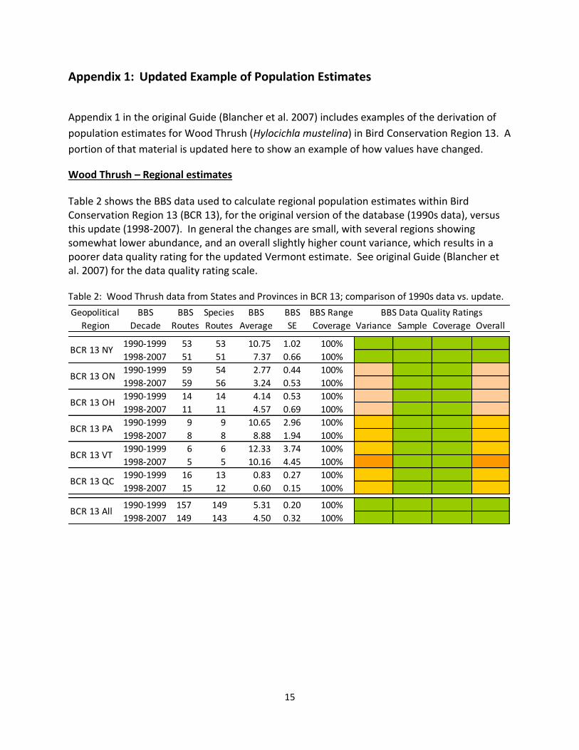
Appendix 1: Updated Example of Population Estimates

Appendix 1 in the original Guide (Blancher et al. 2007) includes examples of the derivation of

population estimates for Wood Thrush (Hylocichla mustelina) in Bird Conservation Region 13. A

portion of that material is updated here to show an example of how values have changed.

Wood Thrush – Regional estimates

Table 2 shows the BBS data used to calculate regional population estimates within Bird Conservation Region 13 (BCR 13), for the original version of the database (1990s data), versus this update (1998-2007). In general the changes are small, with several regions showing somewhat lower abundance, and an overall slightly higher count variance, which results in a poorer data quality rating for the updated Vermont estimate. See original Guide (Blancher et al. 2007) for the data quality rating scale. Table 2: Wood Thrush data from States and Provinces in BCR 13; comparison of 1990s data vs. update.

Geopolitical BBS BBS Species BBS BBS BBS Range

Region Decade Routes Routes Average SE Coverage Variance Sample Coverage Overall

1990-1999 53 53 10.75 1.02 100% 0 Green 0 Green 0 Green 0 Green


1990-1999 59 54 2.77 0.44 100% 1 Beige 0 Green 0 Green 1 Beige




1990-1999 9 9 10.65 2.96 100% 2 Yellow 0 Green 0 Green 2 Yellow



1998-2007 5 5 10.16 4.45 100% 3 Orange 0 Green 0 Green 3 Orange





BCR 13 NY

BCR 13 ON

BBS Data Quality Ratings

BCR 13 OH

BCR 13 PA

BCR 13 VT

BCR 13 QC

BCR 13 All

16

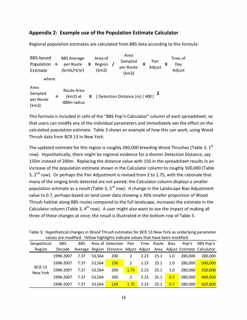
Appendix 2: Example use of the Population Estimate Calculator

Regional population estimates are calculated from BBS data according to this formula:

BBS-based

Population

Estimate=

BBS Average

per Route

(birds/rt/yr)

X

Area of

Region

(km2)

/

Area

Sampled

per Route

(km2)

XPair

AdjustX

Time of

Day

Adjust

where

Area

Sampled

per Route

(km2)

=Route Area

(km2) at

400m radius

X [ Detection Distance (m) / 400 ]2

.

This formula is included in cells of the “BBS Pop’n Calculator” column of each spreadsheet, so

that users can modify any of the individual parameters and immediately see the effect on the

calculated population estimate. Table 3 shows an example of how this can work, using Wood

Thrush data from BCR 13 in New York.

The updated estimate for this region is roughly 280,000 breeding Wood Thrushes (Table 3, 1st

row). Hypothetically, there might be regional evidence for a shorter Detection Distance, say

150m instead of 200m. Replacing the distance value with 150 in the spreadsheet results in an

increase of the population estimate shown in the Calculator column to roughly 500,000 (Table

3, 2nd row). Or perhaps the Pair Adjustment is revised from 2 to 1.75, with the rationale that

many of the singing birds detected are not paired; the Calculator column displays a smaller

population estimate as a result (Table 3, 3rd row). A change in the Landscape Bias Adjustment

value to 0.7, perhaps based on land cover data showing a 30% smaller proportion of Wood

Thrush habitat along BBS routes compared to the full landscape, increases the estimate in the

Calculator column (Table 3, 4th row). A user might also want to see the impact of making all

three of these changes at once; the result is illustrated in the bottom row of Table 3.

Table 3: Hypothetical changes in Wood Thrush estimates for BCR 13 New York as underlying parameter

values are modified. Yellow highlights indicate values that have been modified.

Geopolitical BBS BBS Area of Detection Pair Time Route Bias Pop'n BBS Pop'n

Region Decade Average Region Distance Adjust Adjust Area Adjust Estimate Calculator

1998-2007 7.37 53,564 200 2 2.23 25.1 1.0 280,000 280,000

1998-2007 7.37 53,564 150 2 2.23 25.1 1.0 280,000 500,000

1998-2007 7.37 53,564 200 1.75 2.23 25.1 1.0 280,000 250,000

1998-2007 7.37 53,564 200 2 2.23 25.1 0.7 280,000 400,000

1998-2007 7.37 53,564 150 1.75 2.23 25.1 0.7 280,000 620,000

BCR 13

New York

handbook to the partners in flight population estimates...

Documents