handbook on poverty statistics: concepts …unstats.un.org/unsd/methods/poverty/pdf/un_book final 30...
TRANSCRIPT
1
HANDBOOK ON POVERTY
STATISTICS: CONCEPTS, METHODS
AND POLICY USE
SPECIAL PROJECT ON POVERTY STATISTICS
UNITED NATIONS STATISTICS DIVISION
DECEMBER 2005
2
PREFACE ..................................................................................................................................................... 6 ABOUT THE AUTHORS............................................................................................................................ 8 CHAPTER 1. INTRODUCTION.............................................................................................................. 14
1.1 A BROAD CONSULTATIVE PROCESS.............................................................................................. 15 1.2 ROADMAP.................................................................................................................................... 17
CHAPTER II. CONCEPTS OF POVERTY............................................................................................ 23 INTRODUCTION......................................................................................................................................... 23 2.1 BASIC APPROACHES..................................................................................................................... 27 2.1.1 POVERTY LINES........................................................................................................................... 29 2.1.2 ABSOLUTE VERSUS RELATIVE POVERTY ...................................................................................... 32 2.1.3 COST OF BASIC NEEDS APPROACH .............................................................................................. 33 2.1.4 HOUSEHOLDS AND INDIVIDUALS: ADULT EQUIVALENCE AND SCALE ECONOMIES ....................... 35 2.1.5 ADJUSTMENT FOR NON-FOOD NEEDS........................................................................................... 39 2.1.6 SETTING AND UPDATING PRICES .................................................................................................. 41 2.2 INTERNATIONAL COMPARISONS................................................................................................... 43 2.3 TOWARD HARMONIZATION.......................................................................................................... 47 REFERENCES............................................................................................................................................. 50
CHAPTER III. POVERTY MEASURES ................................................................................................ 52 INTRODUCTION......................................................................................................................................... 52 3.1 DESIRABLE FEATURES OF POVERTY MEASURES ........................................................................... 54 3.2 FOUR COMMON MEASURES.......................................................................................................... 57 3.2.1 HEADCOUNT MEASURE................................................................................................................ 58 3.2.2 POVERTY GAP.............................................................................................................................. 60 3.2.3 WATTS INDEX.............................................................................................................................. 64 3.2.4 SQUARED POVERTY GAP.............................................................................................................. 66 3.3 COMPARING THE MEASURES........................................................................................................ 67 3.4 EXIT TIME AND THE VALUE OF DESCRIPTIVE TOOLS..................................................................... 71 3.5 BROADER CONCERNS................................................................................................................... 78 3.5.1 COMPARISONS WITHOUT POVERTY MEASURES ............................................................................ 78 3.5.2 MEASUREMENT ERROR................................................................................................................ 79 3.6 CONCLUSIONS ............................................................................................................................. 81 REFERENCES............................................................................................................................................. 84
CHAPTER IV. COUNTRY PRACTICES IN COMPILING POVERTY STATISTICS .................... 85 INTRODUCTION......................................................................................................................................... 85 4.1 INCOME- OR EXPENDITURES-BASED MEASUREMENT APPROACHES .............................................. 86 4.1.1 SPECIFY A FOOD POVERTY THRESHOLD ....................................................................................... 87 4.1.2 FOOD BASKET CONSTRUCT AND FOOD POVERTY LINE ( fpl ) ...................................................... 92 4.1.3 ALTERNATIVE APPROACHES TO COSTING A FOOD BASKET: PRICE PER KCALORIE AND HOUSEHOLD
LEVEL fpl ............................................................................................................................................... 95 4.1.4 COMPUTING THE TOTAL POVERTY LINE ( tpl )............................................................................. 96
A. List of specified essential non-food needs...................................................................................... 97 B. Regression 98 C. Engel�s coefficient ....................................................................................................................... 100 D. Comparative performance of the three procedures..................................................................... 101
4.1.5 UPDATING POVERTY MEASURES AND ESTIMATING POVERTY TRENDS........................................ 103 4.1.6 RELATIVE AND SUBJECTIVE INCOME/EXPENDITURES BASED POVERTY LINES ............................ 107 4.2 DIRECT MEASURES OF FOOD POVERTY ...................................................................................... 109
3
4.2.1 ESTIMATING THE EMPIRICAL CUMULATIVE DISTRIBUTION FUNCTION (CDF) OF PER CAPITA ENERGY CONSUMPTION ........................................................................................................................................ 109 4.2.2 HOUSEHOLD SIZE FOR PER CAPITA CALCULATIONS ................................................................... 113 4.2.3 ESCHEWING PER CAPITA CALCULATIONS................................................................................... 116 4.3 NON-INCOME MEASUREMENT METHODS.................................................................................... 117 4.4 CONCLUSION............................................................................................................................. 120 REFERENCES........................................................................................................................................... 125
CHAPTER V. STATISTICAL TOOLS AND ESTIMATION METHODS FOR POVERTY MEASURES BASED ON CROSS-SECTIONAL HOUSEHOLD SURVEYS.................................... 128
INTRODUCTION....................................................................................................................................... 128 5.1 CROSS-CUTTING ISSUES IN POVERTY MEASUREMENT ................................................................ 130 5.1.1 REASONS FOR FAVORING CONSUMPTION EXPENDITURE AS A WELFARE INDICATOR .................. 130 5.1.2 CONSISTENCY OF HOUSEHOLD SURVEY METHODS AND POVERTY COMPARISONS ...................... 135 5.1.3 CORRECTION METHODS FOR RESTORING COMPARABILITY TO INCOMPARABLE SURVEYS .......... 138 5.1.4 MEASUREMENT ERROR IN CROSS-SECTIONAL SURVEY DATA..................................................... 142 5.1.5 VARIANCE ESTIMATORS FOR COMPLEX SAMPLE DESIGNS.......................................................... 145 5.2 TYPES OF SURVEYS.................................................................................................................... 151 5.2.1 INCOME AND EXPENDITURE (OR BUDGET) SURVEYS .................................................................. 151 5.2.2 CORRECTING OVERSTATED ANNUAL POVERTY FROM SHORT REFERENCE PERIOD HIES AND HBS
DATA ......................................................................................................................................... 156 5.2.3 LIVING STANDARDS MEASUREMENT STUDY SURVEYS ............................................................. 159 5.2.4 CORE AND MODULE DESIGNS..................................................................................................... 163 5.2.5 DEMOGRAPHIC AND HEALTH SURVEYS..................................................................................... 164 5.3 PRICING AND UPDATING THE VALUE OF POVERTY LINES............................................................ 167 5.3.1 SPATIAL PRICE DEFLATORS........................................................................................................ 168 5.3.2 WHOSE COST OF LIVING?........................................................................................................... 172 5.3.3 USING PRICES TO IMPUTE THE VALUE OF CONSUMPTION ........................................................... 175 5.3.4 PRACTICAL ISSUES IN COLLECTING PRICE DATA ........................................................................ 177 5.4 ASSESSING INDIVIDUAL WELFARE AND POVERTY FROM HOUSEHOLD DATA .............................. 184 5.4.1 EQUIVALENCE SCALES .............................................................................................................. 186 5.4.2 THE ROTHBARTH METHOD OF MEASURING CHILD COSTS........................................................... 191 5.4.3 THE ENGEL METHOD OF MEASURING CHILD COSTS.................................................................... 194 5.4.4 THE ENGEL METHOD OF MEASURING SCALE ECONOMIES........................................................... 195 5.4.5 ADJUSTING POVERTY STATISTICS WHEN ADULT EQUIVALENTS ARE UNITS ................................ 197 5.4.6 METHODS FOR ESTIMATING THE INTRA-HOUSEHOLD ALLOCATION OF CONSUMPTION............... 198 5.4.7 COLLECTING NON-MONETARY DATA ON INDIVIDUALS TO ESTIMATE GENDER-SPECIFIC MEASURES
OF POVERTY .............................................................................................................................. 200 5.5 CONCLUSION............................................................................................................................. 201 REFERENCES........................................................................................................................................... 203
CHAPTER VI. STATISTICAL ISSUES IN MEASURING POVERTY FROM NON-HOUSEHOLD SURVEYS SOURCES.............................................................................................................................. 206
INTRODUCTION....................................................................................................................................... 206 6.1 PROSPECTS FOR EXPANDING THE POVERTY DATABASE ............................................................. 208 6.2 LIMITATIONS OF HOUSEHOLD SURVEYS FOR POVERTY ASSESSMENT ....................................... 210 6.3 INTEGRATING DIFFERENT DATA TECHNIQUES AND SOURCES ................................................... 213 6.4 MULTI-DIMENSIONAL NATURE OF POVERTY............................................................................. 215 6.5 POVERTY MEASURES AND THE MILLENNIUM DEVELOPMENT GOALS ....................................... 218 6.5.1 RELEVANCE OF THE MDGS....................................................................................................... 219 6.5.2 SIGNIFICANCE OF NON-MARKET GOODS AND SERVICES ............................................................. 220 6.6 PROBLEM OF DETERMINING CAUSES AND EFFECTS ................................................................... 221 6.7 DATA MINING FROM ADDITIONAL SOURCES OF INFORMATION................................................ 223 6.7.1 QUANTITATIVE SOURCES........................................................................................................... 223
A. Censuses, sample censuses, and partial censuses ...................................................................... 223 B. Ministerial reports and administrative records.......................................................................... 230
4
C. Civil registration systems and electoral registers ...................................................................... 235 D. Core Welfare Indicators Questionnaire [CWIQ]........................................................................ 237 E. Special enquiries and official commissions ................................................................................ 241
6.7.2 QUALITATIVE STUDIES AND PARTICIPATORY ASSESSMENTS .................................................... 242 A. Understanding the story behind the numbers ............................................................................. 242 B. Participatory Assessments .......................................................................................................... 244 C. Qualitative methods.................................................................................................................... 246 D. Other non-quantitative methods................................................................................................. 250
6.7.3 NATIONAL ACCOUNTS............................................................................................................... 256 A. Comparability between national accounts and household survey estimate of final household consumption and the concept of household actual final consumption .............................................. 258 B. Conceptual adjustments of household final consumption expenditure between household budget survey and national accounts............................................................................................................ 264 C. Empirical adjustments of household-consumption expenditure between household budget surveys and national accounts ....................................................................................................................... 270
6.8 MAPPING POVERTY CHARACTERISTICS..................................................................................... 275 6.8.1 PIECING THE PUZZLE TOGETHER................................................................................................ 275 6.8.2 DRAWING ON APPROPRIATE INDICATORS .................................................................................. 278 6.9 CONCLUSION............................................................................................................................. 279 ENDNOTES .......................................................................................................................................... 286
E.1. Social transfers in kind (SNA, para. 9.72)................................................................................. 286 Social transfers in kind include: ....................................................................................................... 286 E.2. Household production for own final consumption..................................................................... 286 E.3. Additional data for measuring household final consumption.................................................... 287
REFERENCES........................................................................................................................................... 289 CHAPTER VII. POVERTY ANALYSIS FOR POLICY USE: POVERTY PROFILES AND MAPPING................................................................................................................................................. 292
INTRODUCTION....................................................................................................................................... 292 7.1 POVERTY MONITORING AND POVERTY PROFILES ....................................................................... 294 7.1.1 CAPABILITY DEPRIVATION ........................................................................................................ 302 7.1.2 PRODUCTIVE ASSETS HELD BY POOR AND NON-POOR ................................................................ 308 7.2 POVERTY MAPPING.................................................................................................................... 309 7.3 SOME LIMITATIONS IN POVERTY MAPPING AND ALTERNATIVE WITHOUT CENSUS DATA ............ 314 7.4 PRACTICAL ISSUES OF IMPLEMENTING GEOGRAPHICAL TARGETING .......................................... 318 REFERENCES........................................................................................................................................... 322 APPENDIX............................................................................................................................................... 323
CHAPTER VIII. ANALYSIS OF POVERTY DYNAMICS ................................................................ 324 INTRODUCTION....................................................................................................................................... 324 8.1 CONCEPTUAL ISSUES ................................................................................................................. 325 8.1.1 RELATIONSHIP BETWEEN INEQUALITY AND MOBILITY............................................................... 326 8.1.2 CHRONIC VS. TRANSIENT POVERTY ........................................................................................... 328 8.1.3 COMPARING INCOME GROWTH AMONG POOR AND NON-POOR HOUSEHOLDS .......................... 333 8.2 DATA ISSUES ............................................................................................................................. 334 8.2.1 PANEL DATA VERSUS REPEATED CROSS-SECTIONAL DATA...................................................... 334 8.2.2 MEASUREMENT ERROR ............................................................................................................. 336 8.3 RECOMMENDATIONS FOR DATA COLLECTION........................................................................... 342 8.4 ANALYTICAL METHODS WITH EXAMPLES .................................................................................. 345 8.4.1 REPEATED CROSS-SECTIONAL DATA (INCLUDING POVERTY MONITORING) ................................ 345 8.4.2 PANEL DATA FOR TWO POINTS IN TIME ...................................................................................... 352 8.5 CONCLUSION............................................................................................................................. 365 REFERENCES........................................................................................................................................... 368
CHAPTER IX. CONCLUSION .............................................................................................................. 370 9.1 SUMMARY ................................................................................................................................. 370
5
9.2 STATISTICAL ADDENDUM: THE UN GLOBAL SURVEY ON POVERTY MEASUREMENT PRACTICES 373 ANNEXES................................................................................................................................................. 375
A.1 LIST OF THE UNITED NATIONS STEERING COMMITTEE ON POVERTY STATISTICS ............................ 375 A.2 LIST OF THE COUNTRIES WHO PARTICIPATED IN THE REGIONAL WORKSHOPS ON POVERTY MEASUREMENT....................................................................................................................................... 377 A.3 QUESTIONNAIRE OF THE UN GLOBAL SURVEY OF POVERTY MEASUREMENT PRACTICES AND STATISTICAL ADDENDUM ....................................................................................................................... 378
6
PREFACE
Poverty is multifaceted, manifested by conditions that include malnutrition,
inadequate shelter, unsanitary living conditions, unsatisfactory and insufficient supplies
of clean water, poor solid waste disposal, low educational achievement and the absence
of quality schooling, chronic ill health, and widespread common crime. Through the
signing of the Millennium Development Declaration in 2000, 191 UN member states
unanimously committed to reducing poverty. However, because it is not easy to define or
measure, monitoring poverty in its broad manifestations is a complex task conceptually
and empirically.
The provision of benchmark data needed for monitoring global targets rests on
national statistical offices, and meeting the current demands for poverty statistics is still
beyond the reach of most poor countries. The current status of reporting on the indicators
of the major UN global conferences - and more recently - the follow up of the
Millennium Development Goal (MDG) targets, raises concerns about the readiness of
national statistical offices to respond to this demand. A review of countries practices of
poverty measurements reveals that there is no uniform standard in the way countries
collect and process their data and there are large gaps in the development of poverty
statistics among the countries. With regard to the overall findings, however, current
practices show important similarities, with some variations as well. Poverty estimates
based on dietary caloric intake, for example, are well conceptualized and implemented
with a fair degree of consistency within regions and to some extent across regions.
This handbook is the first United Nations publication on the methodology of
assessing poverty. In line with the goals set forth by the Millennium Declaration, The
United Nations Statistics Division�s immediate concern is to strengthen each country�s
capacity to provide fundamental, consistent statistical information on poverty:
• How much poverty is there?
• Who are the poor?
7
• What are the characteristics of their living conditions? and
• How does poverty evolve over time?
These apparently simple questions involve complex responses. The most practical
challenge is attributable to the differences in national conditions and policy needs,
evidenced across the globe in the wide range of measurement practices.
The handbook provides a comprehensive review of the current practices of
poverty measurement worldwide and sketches a road to improving country practices
while achieving greater comparability within and across countries. It is hoped that this
book will serve as the basis for formulating national, regional and international statistical
programs to strengthen the capacity in member countries to collect and analyze data.
Our hope is that better data can directly improve national and international policies aimed
at reducing poverty globally.
Paul Cheung, Director
United Nations Statistics Division
8
ABOUT THE AUTHORS
Gisele Kamanou1 is Editor and Project Manager of the Special Project on
Poverty Statistics at the United Nations Statistics Division. She initiated, coordinated, and
managed the publication of this handbook and related activities since its launch in 2003.
Gisele Kamanou received her Ph.D. in Bio Statistics from the University of California at
Berkeley and has taught statistics at Columbia University. The main focus of her research
is the measurement of poverty and analysis of household-level data. Her most recent
work involved developing methods for combining cross-country development indicators
using modern statistical modeling techniques, of which models with mixed discrete and
continuous data. She coauthored �Measuring Vulnerability to Poverty,� a chapter
published in Insurance Against Poverty, edited by Stefan Dercon, Oxford University
Press, 2003, pp. 155-175.
Jonathan Morduch is Associate Professor of Public Policy and Economics at the
Wagner Graduate School of Public Service at New York University, where he teaches on
the economic and social development in low-income countries. His research focuses on
poverty and inequality, and has developed tools for measuring vulnerability,
decomposing inequality, and relating poverty reduction to growth processes. Morduch�s
recent research centers on poverty reduction through microfinance, and he is the co-
author of The Economics of Microfinance with Beatriz Armendariz de Aghion (MIT
Press, 2005). Jonathan Morduch has taught on the Economics faculty at Harvard
1 I wish to acknowledge the contribution and support of my colleagues in United Nations Statistics Division and in particular that of Christoff Paparella and Stefan Schweinfest.
9
University, was a National Fellow at the Hoover Institution at Stanford University, a
MacArthur Foundation Research Fellow at Princeton University, and an Abe Fellow at
the University of Tokyo. Morduch received his Ph.D. in Economics from Harvard
University.
Isidoro P. David received his Ph.D. in statistics from Iowa State University. He
taught at Ohio State University and University of the Philippines and later joined the
Asian Development Bank where he retired as chief statistician in 2000. His work at ADB
included formulating and directing technical assistance for improving statistical systems
of Asian and Pacific developing countries. He was President of the Philippine Statistical
Association, Vice-President of the International Association of Survey Statisticians, and
Council Member and Chair of the Agriculture Statistics Committee of the International
Statistical Institute. He served in various scientific program committees of the ISI and its
satellite associations. Since retiring from ADB, Dr. David has done consulting work for
various countries and international agencies, including ADB, FAO, UNDP, UNSD, UN-
ESCAP and World Bank. He chairs the Technical Committee on Survey Design of the
Philippine statistical system and is adjunct professor at the University of the Philippines
at Los Baños.
John Gibson is Professor in the Department of Economics at the University of
Canterbury, New Zealand, where he teaches microeconomics of development and
econometrics. His research focuses on poverty and the behavior of households in low-
10
income settings. His research also studies the effect that different data collection
methods can have on measurement error in surveys of living standards.
Professor Gibson has taught in the Economics Department at the University of Waikato
in New Zealand, and in the Economics Department and Center for Development
Economics at Williams College in the United States. He received his Ph.D. from the
Food Research Institute of Stanford University.
Ivo Havinga is Chief of the Economic Statistics Branch at the United Nations
Statistics Division.
Michael Ward has had a long career with UN institutions and The World Bank
where he developed a special interest in the inter-related questions of poverty, inequality,
and social disadvantage. He has published widely on statistical matters and is the author
of the �Quantifying the World� volume in the UN Intellectual History series.
to 1999. He received his Ph.D. in Economics from Stanford University in 1985.
Nanak Kakwani is presently the Director and Chief Economist of the
International Poverty Centre in Brasilia , Brazil. Before joining IPC, he was a professor
of Econometrics at the University of New South Wales in Sydney , Australia for 30
years. His research has focused on econometrics, poverty, inequality, pro-poor growth,
taxes, public policies, and health economics. Professor Kakwani has written more than
100 articles published by various international journals and is the author of �Analyzing
11
Redistribution Policies: A Study Using Australian Data, Cambridge University Press
1986� and �Inequality and Poverty: Methods of Estimation and Policy Applications,
Oxford University Press 1980�. He was a fellow in Australian Research Committee of
Social Science. He was also awarded Mahalanobis gold medal by the Indian Econometric
Society for outstanding contribution in quantitative economics.
Hyun H. Son is a poverty specialist at UNDP-International Poverty Centre in
Brasilia, Brazil. She has a Ph.D. in Economics. Dr. Son worked for the World Bank in
Washington, DC and held an academic position at Macquarie University in Sydney,
Australia. Her research area includes poverty, inequality, pro-poor growth, and public
policy.
Paul Glewwe is Associate Professor of Applied Economics at the University of
Minnesota, where he teaches econometrics and microeconomic analysis of economic
development. His research focuses on education in developing countries, concentrating
on the factors that determine academic outcomes in primary and secondary schools. He
also conducts research on malnutrition, inequality, and poverty in developing countries.
He is the author and editor of four books on these topics and has written over 30
academic journal articles. He has conducted research on China, Cote d�Ivoire, Ghana,
Honduras, Jamaica, Jordan, Kenya, Laos, Malaysia, Morocco, Peru, the Philippines, Sri
Lanka, Turkey, and Viet Nam. Before coming to the University of Minnesota, he was a
research economist at the World Bank from 1986
12
We gratefully acknowledge the important contributions of Michael Bamberger,
Christiaan Goortaert, and Sanjay Reddy--who reviewed and commented on the chapters.
Michael Bamberger has a Ph.D. in Sociology from the London School of
Economics. He worked for 13 years in Latin America with a number of NGOs on poverty
and gender-related programs and evaluations. During his 22 years with the World Bank,
he was adviser on monitoring and evaluation of the urban development program, where
he also conducted studies on interhousehold transfers and survival strategies of the urban
poor. Since retiring from the World Bank in 2001, Mr. Bamberger has been a consultant
to the UNDP, UN-DESA, USAID, the World Bank, and DFID on a range of subjects
relating to poverty, program evaluation, and the MDGs.
Christiaan Grootaert has a Ph.D. in Economics and recently retired after 23
years of service at the World Bank. He was Lead Economist in the World Bank�s Social
Development Department, and Manager of the Social Capital Initiative, which sponsored
empirical studies on the effects of social capital in 15 countries. During his career, Mr.
Grootaert researched the measurement and analysis of poverty, risk and vulnerability,
education and labor markets, child labor, and the role of institutions and social capital in
development. He has published widely in these areas and provided policy advice to
governments in Africa, Asia, Eastern Europe, and the Middle East. He recently
coauthored several books with T. van Bastelaer--The Role of Social Capital in
Development: An Empirical Assessment [Cambridge University Press] ] and Understanding
and Measuring Social Capital: A Multidisciplinary Tool for Practitioners [The World
13
Bank]. And he was the co-author of the World Development Report 2000/2001: Attacking
Poverty. Mr. Grootaert is currently an international development consultant.
Sanjay Reddy is an Assistant Professor of Economics at Barnard College,
Columbia University. His areas of work include development economics, international
economics, economics and philosophy, and economics and social theory. He is the co-
author of "How Not to Count the Poor". Prof. Reddy possesses a Ph.D. in economics
from Harvard University, an M.Phil. in social anthropology from the University of
Cambridge, and an A.B. in applied mathematics with physics from Harvard University.
He held several positions as consultant for development agencies and international
institutions, including the ILO, Oxfam, UNICEF, UNDP, UNU-WIDER and the World
Bank.
We would like to also thank members of the Steering Committee on Poverty
Statistics for their contribution in the early phases the Poverty Statistics Project, in
particular for their comments on the preliminary outline of the book. We acknowledge
the invaluable contribution of countries who participated in the regional workshops and,
in particular, those who shared their practices and made available their data which were
used to exemplify improvements but also difficulties countries still face in compiling
poverty statistics. The list of the members of the UN Steering Committee on poverty
statistics and that of the participating countries in the regional workshops are provided in
the Annexes at the end of the book.
14
CHAPTER 1. INTRODUCTION
Gisele Kamanou
Hundreds of millions of people struggle with poverty around the world. Their
plight may be obvious to the eye, but statisticians have had to labor hard to create
reliable, consistent, and comparable measures of poverty. Being poor is generally viewed
in terms of deprivation of some of life�s basic needs, such as food, shelter, clothing, basic
education, primary health care, and security. But accurately measuring these indicators is
no simple task, and philosophers still debate specifics of definitions. Balancing
philosophical understandings against the practical needs and constraints faced by national
statistical offices has been challenging, but great progress has been made in the past
several decades. This handbook is dedicated to furthering the process of improvement.
Governments around the world define and measure poverty in ways that reflect
their own circumstances and aspirations. Income is universally an important element,
even while most agree that money metrics are too narrow to capture all relevant aspects
of poverty. Still, the challenges of measuring poverty narrowly defined by a lack of
money are substantial in themselves, and statistical offices have adopted a wide array of
methodological approaches. These methodological choices can matter greatly, and the
ultimate users of data are usually left unaware of which choices were made and how they
matter. Without that knowledge, it is impossible to make fully reliable comparisons of
15
poverty rates across countries, or even to confidently compare rates for a single country
across different years.
To assist countries in responding to the increasing demand of poverty monitoring,
the United Nations Statistics Division (UNSD) launched in 2003 a Special Project on
Poverty Statistics with the ultimate goal being the preparation of this Handbook on
Poverty Statistics: Concepts, Methods and Policy Use. The next section describes the
process put into place to prepare the Handbook and the following one defines its scope
and contents, together with suggestions on how best to use the Handbook.
1.1 A broad consultative process
Four regional workshops--in Latin America and the Caribbean (May 2004),
Africa (July 2004), Asia and the Pacific (October 2004), and in the ESCWA countries
(November 2004)--on poverty measurements were conducted to support the drafting of
the handbook�s chapters. The specific objectives of the workshops were to discuss the
content of the handbook with countries to incorporate practical regional perspectives and
to identify common problems countries face in this area. UNSD also implemented a
global survey of poverty measurement approaches in 2005 to gauge the range of ways
poverty is measured. A questionnaire based on current measurement practices was
developed and sent to all countries worldwide (see Chapter 9 for a more details on the
survey and the questionnaire in the Annexes at the end of the book). An expert group
16
consisting of authors and chapter reviewers met in New York in June 2005 to
comprehensively review the first draft of the handbook.
This review of national poverty measurement practices from around the globe
showed that the basic needs approach to poverty assessment has gained highest
acceptance among the developing countries. Basic needs are grouped broadly into food
and non-food, while the income approach to measurement involves estimating the costs
of the two groups. The review however, showed a wide range of practices. For example,
the data reveal that 63 percent of 91 respondent countries apply the absolute concept of
poverty (41 countries responded that they use the absolute concept of poverty only and 16
other said both absolute and relative). Likewise there is a wide range of practice among
the 69 countries (for who adjusting for adult equivalent was applicable) who indicated
whether or not they make adjustments for adult equivalence in their poverty analyses
with 23 countries (33 percent) making some kinds of adjustments for age and/or sex.
Noteworthy is the difference in the minimum calorie requirement for an individual which
ranges from below 2000 kilocalories to close to 3000 kilocalories in some cases. The
thresholds spread almost uniformly between these two values, with a slight mode (17
countries) having a threshold between 2100 and 2300 kilocalories.
A complement of the income-based basic needs approach is the so-called
minimum basic needs (MBN) or unmet basic needs (UBN) approach. In the latter, non-
monetary indicators representing different dimensions of poverty are chosen, estimated,
and monitored. A few numbers of countries the UNSD surveyed also collect data on
17
�unmet basic needs.� Methods here are still being developed, and there is much less
uniformity of practice than there is around the analysis of income and spending-based
poverty measures. The three broad categories of basic needs often considered are
dwelling characteristics, access to safe water, and access to sanitation facilities. Basic
education and economic capacity (e.g., GDP growth rate) are sometimes included in an
expanded UBN set of indicators. Most commonly, statisticians calculate an index of
deprivation that combines the degrees of access to the various components.
Together, the data show a broad consensus about the guiding principles
underlying poverty measurement in monetary terms. They also revealed, however,
considerable variation in how the principles are implemented in practice. Reliable and
comparable data are critical for poverty reduction policies. Much progress has already
been made in improving data collection and measurement methods around the world, and
this handbook seeks to add to these improvements.
1.2 Roadmap
The handbook focuses on issues confronting developing countries. It provides
these countries with practical measurement options, taking regional and local specificities
into consideration to the extent possible. While it does not offer new concepts or
methods, the handbook�s strong methodological component will serve as a foundation for
empirical work conducted at the country level.
18
The target audience of the handbook are statisticians at government offices who
possess an intermediate to strong background in statistics, with significant familiarity
with common statistical modeling techniques such as regression or principal components
analysis. Some chapters of the handbook require an advanced level of statistical theory
whereas others are targeted to policy makers with minimal statistical literacy.
The publication is composed of nine chapters covering both theoretical and
applied work. On of the fundamental addition of this Handbook to the traditional manuals
on poverty statistics is its emphasis on practical issues while also addressing keys
methodological issues in poverty measurements.
Chapters 2 and 3 delineate the key issues in poverty analysis based on income and
consumption measures. They summarize the literature on advanced theories on poverty
indices with a focus on their implications for empirical studies. Chapter 2 begins by
noting the diversity of approaches to poverty measurement that are employed around the
world. In seeking a basis for achieving greater uniformity, the chapter introduces issues
around the setting of poverty lines and adjustments made for the age and gender
composition of households. One way to achieve greater comparability of measures is to
use �international poverty lines� such as the $1/day per person lines incorporated in the
United Nations Millennium Development Goals. The $1/day lines have strengths and
limits, but ultimately they cannot replace a country�s own poverty assessments. The
conclusion to chapter 2 highlights areas of concern in improving (and unifying) country-
specific approaches.
19
Chapter 3 starts off with a basic discussion of poverty measurement for readers
unfamiliar with the subject. However, readers with experience on poverty measurements
or users of poverty statistics would find these sections useful for understanding some
fundamentals of assessing poverty, which supports the more in depth discussions that
occur in Chapters 5 and 6. The chapter describes commonly-used poverty measures such
as the headcount, poverty gap, and the squared poverty gap. The first part of the chapter
shows how the measures weigh different degrees of deprivation. The second part of the
chapter describes a new and complementary approach to poverty measurement based on
the time before exit from poverty due to steady income growth. The conclusion argues
that publishing simple statistics such as the median income of the poor population can be
a useful addition to traditional poverty measures.
Chapter 4 discusses current practices of measuring poverty in developing
countries, summarizing the experiences of individual nations presented during the four
regional workshops organized in support of the handbook. The steps involved in
measuring poverty are discussed and analyzed systematically, and practical difficulties
met in implementing some of the steps are pointed out. Alternative ways of solving or
circumventing some of these difficulties are proposed, with particular reference to food
poverty statistics. The chapter highlights the major sources of non-comparability of
poverty statistics, exploring ways for harmonizing the practice of measuring poverty
across countries to improve comparability of poverty statistics.
20
Chapters 5 and 6 study the sources of data for poverty statistics, herein referred to
as survey and non-survey sources. Chapter 5 is written primarily for statisticians at
national statistical offices who have the responsibility of developing standards and
methods for data collection based on sampling techniques used by themselves or by other
government entities such as line ministries. The chapter focuses on techniques and broad
statistical considerations for generating reliable, comparable estimates of income,
consumption, and other monetary and non-monetary assets. It describes methods and data
for measuring poverty with cross-sectional household surveys. It starts by examining
several issues that are independent of the type of survey used: cross-survey
comparability, measurement error, and variance estimators for complex sample designs.
It then analyzes the different types of cross-sectional surveys available, in terms of their
suitability for poverty analysis. The chapter also considers the need for information on
prices when measuring poverty and the difficult issues involved in assessing individual
welfare and poverty from household data.
Chapter 6 is designed for a broader set of users, including non-survey statisticians
and other statisticians/data analysts without a strong background in modern statistical
theory. This chapter deals with certain limitations of household surveys for gathering data
relating to all the dimensions of poverty and where poor people can be found. It reviews
the relevance of various administrative and non-household survey sources for filling in
the gaps and for amplifying existing survey data on poverty in the context of the
Millennium Development Goals. The chapter also addresses the policy debate
surrounding use of national account for compiling poverty levels. Conceptual and
21
empirical differences between estimates of household consumption based on national
accounts versus household surveys are examined. Adjustments necessary to reconcile the
two estimates are then presented. Statisticians who compile data in line ministries and
statistical assistants in community-based registries, for example, will find practical
guidance on how best to utilize their data. In general, the chapter cautions on the limits of
non-survey data in poverty analysis.
In targeting data analysts and policy makers, Chapter 7 discusses poverty
profiling and poverty mapping and Chapter 8 focuses on poverty dynamics. Both
chapters present analytical techniques with country-level illustrations on how to use
poverty statistics to formulate national policy. Familiarity with interpretation of basic
statistical concepts, such as ratio, rate, and bias, is required. Some initial knowledge of
policy-targeting issues is also necessary to fully benefit from these two chapters�
findings. The main focus of Chapter 7 is the formulation of poverty reduction policies. It
shows how various statistical tools, specifically poverty profiles and mapping, can be
used to strengthen the impact of government programs and spending on poverty
alleviation. The chapter thus provides some country-specific examples to illustrate how
poverty profiles can be constructed and how they can be utilized to design policies. The
chapter also provides a review of methodology used in the construction of poverty
mapping, another important tool used by many governments to target the provision of
basic services, in particular education and health.
22
Chapter 8 continues the discussion begun in Chapter 7 by analyzing changes in
poverty over time. It examines three important conceptual issues in poverty analysis: the
relationship between income inequality and poverty at a single point in time and income
mobility over time, the distinction between chronic and transient poverty, and the
measurement of income growth among the poor. It discusses the relative merits of panel
data and repeated cross-sectional data, and the problem of measurement error in income
and expenditure data. It concludes by providing practical country examples of how to
analyze poverty dynamics using data from Indonesia, Papua New Guinea, Russia and
Vietnam.
Chapter 9 concludes the handbook by recommending some basic steps that should
be followed for improving accuracy of poverty statistics while fostering a harmonized
approach for collecting and comparing data across time and space.
23
CHAPTER II. CONCEPTS OF POVERTY
Jonathan Morduch
Introduction
Nelson Mandela came out of retirement in February 2003 to speak on behalf of
the Make Poverty History campaign in London, an effort to renew the global commitment
to eliminating poverty worldwide. �Like slavery and apartheid, poverty is not natural,�
Mandela intoned. �It is man-made, and it can be overcome and eradicated by the action
of human beings.� In imagining a world without poverty, Mandela echoed arguments
first made by reformers like Paine and Condorcet in the wake of the French Revolution
(Stedman Jones, 2004). Writing of an imminent effort to fight global inequality,
Condorcet wrote in 1793 that �everything tells us that we are now close upon one of the
great revolutions of the human race.�2 Condorcet�s great revolution remains unrealized
two centuries later, and advocates hope that Mandela�s strong voice will spur surer action
to eliminate the deprivations suffered by the world�s poor.
In turning from a moral case to the practical task, the initial questions are:
o How do we go from advocacy to action?
o What are the most important constituents of poverty?
2 Antoine-Nicolas de Condorcet, Sketch for a Historical Picture of the Progress of the Human Mind, 1795, as cited in Stedman-Jones (2004), p. 17.
24
o How can elements of deprivation be addressed that go beyond a lack of
private resources?
o How, as a practical matter, should poverty be officially defined and
measured in a world where technical and administrative capacities are
often limited, especially where national statistical offices are already
stretched thin?�
Experts have long-debated the philosophical foundations of what it means to be
poor. But for all of the precision of language and concept, it is a different matter entirely
to apply philosophies to data and implement concepts that appear so crystalline on paper.
The world of poverty measurement in practice is one of compromise, of short-cuts and
approximations. This handbook is devoted to improving the practice of compromise and
approximation, to making choices more transparent, and to identifying seemingly minor
methodological points that can have major implications for measured outcomes.
Compromise and approximation turn out to be critical matters. Researchers have
found, for example, that changing assumptions about data collection and measurement
methods can dramatically alter the poverty rate in Latin America�raising measured
poverty rates from 13 percent of the region to 66 percent. In the process, 250 million
people go from being counted as non-poor to poor (Székely, et al, 2000). The same
researchers describe how differences in assumptions led one set of researchers to find
poverty to be as low as 20 percent of the population of Mexico in 1994, while another set
of researchers found poverty to be as high as 46 percent. This difference shifts 25 million
25
people from one side of the poverty line to the other�even though both sets of
researchers were analyzing the same household survey.
Governments around the world have found it useful to define and measure
poverty in ways that reflect their own circumstances and aspirations. But a historical
assessment suggests that, on balance, greater uniformity of practice will be a major step
forward. One unintended consequence of the various indigenous methods of survey
collection in practice today is the difficulty of comparing poverty measures across
countries and across time. The lack of uniformity also makes it difficult to confidently
integrate country-level poverty measures to gain an overall sense of regional and global
poverty. At present, even basic parameters are treated very differently around the world.
Lack of purchasing power is universally an important element, for example, but some
statistical offices measure purchasing power as income and others measure it as
expenditures. Within each definition (income or expenditures), an even greater diversity
of approaches are employed. Wide differences arise in the setting of poverty lines, for
example, as well as variations in the types of data collected, survey methods, and ways
data are aggregated to create poverty measures.
Questions of measurement are not matters of mere description. The way that
poverty is gauged affects how policy questions are conceptualized, how groups are
targeted, and how countries determine progress in improving living standards. The
implications go beyond any given country at any given moment; they are critical for
future understandings, and for identifying how other countries consider, through
26
comparison, their own conditions and possibilities. Transparent, consistent poverty
measures based on transparent, consistent survey data are thus an international concern.
However, few methodological choices are completely obvious, and the result to date has
been a wide-range of practices with limited comparability.
The United Nations Statistical Division (UNSD) implemented a global survey of
approaches in 2004-5 to gauge the range of ways poverty is measured. By the end of
2005, government statistical offices in 93 countries provided detailed responses to the
survey. Of these countries, 62 completed a slightly longer �expanded� survey with a
broader set of questions.3 The survey was accompanied by four regional meetings also
organized by the UNSD (in Latin America, Africa, Asia, and Europe). Together, the data
show a broad consensus about the guiding principles underlying poverty measurement.
They also reveal, however, considerable variation in how the principles are implemented
in practice. As described throughout this handbook, these details matter, often to a
surprising degree.
This chapter and the handbook as a whole identify and build on the areas where
there is broad consensus. While identifying important variations in implementation, this
book explores ways to build greater consensus in international practice by translating
3 Responses to the longer survey were received by May 2004. The 62 countries included Albania, Armenia, Australia, Austria, Bahamas, Belarus, Burkina Faso, Cambodia, Cameroon, Canada, Croatia, Cyprus, Czech Republic, Denmark, Dominica, El Salvador, Finland, France, Gambia, Germany, Greece, Iran, Iraq, Ireland, Israel, Jordan, Kazakhstan, Kenya, Lithuania, Macedonia, Madagascar, Malawi, Maldives, Mauritius, Mexico, Moldova, Mongolia, Morocco, Nepal, Netherlands, Norway, Oman, Palestine, Paraguay, Philippines, Poland, Russian Federation, St. Kitts and Nevis, Senegal, Sierra Leone, Slovokia, Spain, Suriname, Sweden, Tajikstan, Thailand, Turkey, Uganda, United Kingdom, Ukraine, Vietnam, and Zanzibar.
27
principles into action. Section 2.1 discusses issues involved in establishing and updating
poverty lines. Section 2.2 describes debates around the international �$1/day� poverty
line, and Section 2.3 describes possibilities for harmonizing approaches.
2.1 Basic approaches
The earliest definitions of poverty centered on the inability to obtain adequate
food and other basic necessities. Today, the main focus continues to be on material
deprivations, i.e., the failure to command private resources. Development experts,
including Sen (1987), though, have argued that this notion of economic welfare remains
too narrow to reflect individual well-being, spurring active efforts over the past several
decades to expand the concept of poverty.
One direction of expansion begins with recognition that even material
deprivations may involve more than lack of private resources. If a village has no wiring
for electricity, residents can have substantial income but no steady power source. If
quality health facilities do not exist, no amount of money may be enough to purchase
effective, convenient care.
One direction is thus to use household surveys and community-based
questionnaires to ascertain a population�s access to basic services, irrespective of
household incomes. About 14 percent of respondents to the UNSD �expanded� survey
collect data on such �unmet basic needs� (56 statistical offices responded to the
28
question). Among the focuses are housing conditions, water, sanitation, electricity,
education, and infrastructure. Most commonly, statisticians calculate an index that
combines the degrees of access to the various components. They then describe
deprivations according to cut-off points in the index. Methods here are still being
developed, and there is much less uniformity of practice than around the analysis of
income and spending-based poverty measures. Still, even the emerging efforts are a
reminder that household budgets tell only one part of a story.
A second direction of expansion includes collecting data on household-level
deprivations along dimensions other than money. Researchers, for example, have
focused on social deprivations: the inability to fully participate in communities and,
perhaps, in religious life. They have also focused directly on physical deprivations, such
as those caused by disability, disease, and under-nutrition. And, increasingly, policy
makers have recognized that one part of what it means to be poor resides in a sense of
vulnerability to devastating loss--living on the edge of adequacy with its attendant
uncertainties.
Not surprisingly, a single, all-encompassing measure of poverty remains beyond
reach. One response is to turn to methods like �participatory rural assessments� (which
can be applied as well to urban areas). The idea in this approach is to ask members of a
village or neighborhood to define their own poverty standards and to identify who would
be judged poor according to that notion. The appeal of this approach is that it
accommodates local ideas and conditions; the disadvantage is that it could produce
29
various, noncomparable standards. Moreover, the results typically yield only a reckoning
of who is poorer than who, rather than an absolute measure of poverty against a fixed
benchmark.
Recognizing the trade-offs, researchers are now seeking compromises by
integrating qualitative and quantitative indicators into their analyses. While important in
itself, the qualitative data can also provide a helpful check on the robustness of lessons
learned from traditional quantitative analyses. The ongoing challenge faced by
statisticians and researchers (no matter which techniques they employ) is how to capture
important elements of poverty in transparent, reliable, and practical ways.
2.1.1 Poverty Lines
Despite the breadth of concerns, social scientists still find it useful to focus largely
on poverty as a lack of money�measured either as low income or as inadequate
expenditures. One reason for focusing on money is practical: inadequate income is clear,
measurable, and of immediate concern for individuals. Another reason is that low
incomes tend to correlate strongly with other concerns that are important but harder to
measure. Those in the worst health and with the lowest social status, for example, tend
also to come from the bottom of the income distribution. Lack of money serves as a
rough but quantifiable proxy for a host of deprivations. Thus, narrow definitions of
30
poverty claim particular attention throughout the handbook, even as income and
expenditure are understood to determine only part of overall well-being.4
Even within the narrow sphere of money-based measures, substantial questions remain
about how to proceed, and practices differ widely from country to country. There is no
consensus, for example, on whether money-based measures should focus on income
levels or on spending patterns. Poverty can be measured either by a lack of income or by
a shortfall in expenditures. While they are closely related conceptually, they can
sometimes be quite far apart quantitatively. The 2004-5 survey by UNSD showed that of
84 countries that responded to the question, almost half base their poverty calculations on
expenditure data, about 30 percent base the calculations on income data only, and 12
percent use both.
The ability to spend is primarily determined by one�s income. But spending and
income are not identical since households also borrow, sell assets, or draw on savings
when income is low. Conversely, households often save when times are especially
favorable. Measuring poverty as a shortfall in spending takes into account these kinds of
coping mechanisms and households� general abilities to �smooth consumption� over
time. A second difference concerns the ease and reliability of data collection. As
described in subsequent chapters, pure statistical issues reinforce the advantages to basing
poverty measures on expenditure data rather than income. As noted above, one purpose
4 The United Nations Millennium Development Goals for 2015 reflect the diversity of objectives through a broad list of primary and secondary goals focusing on deprivations, such as low levels of child and maternal health, education , and basic nutrition.
31
of the handbook is to clarify how these kinds of choices affect measurement�and how
they affect the understanding of poverty.
The usual next step is to identify a poverty line. A poverty line typically specifies
the income (or level of spending) required to purchase a bundle of essential goods
(typically food, clothing, shelter, water, electricity, schooling, and reliable healthcare).
Identifying the poor as those with income (or expenditures) below a given line brings
clarity and focus to policy making and analysis. Having a poverty line allows experts to
count the poor, target resources, and monitor progress against a clear benchmark.
Communicating the extent of poverty becomes easier, and explaining the notion of
deprivation simpler.
Statistical offices spend much time and effort setting and updating poverty lines.
However, the place of poverty lines needs to be put in context. A recent study of 17
Latin American countries, for example, shows that many other elements of poverty
measurement are more important than the choice of poverty lines. These include
adjustments for adult equivalent family size and the treatment of missing data in surveys
(Szekely, et al, 2000).
It is also important to bear in mind differences between concepts and reality. The
fact is that a poverty line (below which one is poor and above which one is not) has little
empirical correspondence in the daily lives of the poor. Researchers analyzing data on
households see no clear breaks or discontinuities in the relationship of income and health
32
or nutrition, and certainly no systematic breaks in living standards that correspond to
poverty lines as the term is used. Yet, poverty measures based on poverty lines serve an
important descriptive purpose and should be seen in that light.
2.1.2 Absolute versus relative poverty
A poverty line indicates deprivation in an absolute sense, i.e., the value of a set
level of resources deemed necessary to maintain a minimal standard of well being. With
such a definition, poverty is eliminated once all households command resources equal to
or above the poverty line. The $1/day per capita poverty line is one example of an
absolute poverty line, but most countries determine their own absolute poverty lines as
well.
Many wealthier countries, on the other hand, set poverty lines based on relative
standards. In the United Kingdom, for example, the poverty line is 60 percent of the
median income level (after taxes and benefits and adjusted for household size), an
approach adopted broadly in the European Union. In 2002/2003, the UK figure
translated into a poverty line of £283 per week (equivalent to $28,418 per year based on
2003 exchange rates) for a household with two adults and two children, a figure
considerably higher than the absolute 2003 poverty line in the United States of $18,400
per year for a similar family.5 The relative benchmarks used in Europe reflect the belief
that important deprivations are to be judged relative to the well-being of the bulk of 5 The US standard translates to $19.46 per day per capita or $7,104 per year per capita. UK data are from http://www.poverty.org.uk/summary/key_facts.htm. US data are from http://aspe.hhs.gov/poverty/figures-fed-reg.shtml. The websites were accessed in June 2005.
33
society, approximated by the income level of the household at the mid-point of the
income distribution. In short, inequality matters as a component of deprivation. As such,
relative poverty can be reduced but never eliminated--except in the extreme (and
implausible) case in which income equality is fully achieved.
When asked in the UNSD survey whether they calculated absolute poverty lines,
two-thirds of statistical offices answered affirmatively. Those that favored relative
approaches were mainly drawn from the OECD, including, for example, Australia,
Canada, Denmark, Ireland, Norway, and the United Kingdom. Where the incidence of
hunger and the inability to obtain basic essentials is more pronounced, however, the
preference strongly favors absolute measures of poverty�and the $1/day or $2/day lines
echo that choice.
2.1.3 Cost of Basic Needs approach
The way in which statistical offices set absolute poverty lines varies considerably.
Most begin with a �cost of basic needs� approach (described in greater detail in Chapters
4 and 5), but the variations in the application of the approach multiply with each step.
The basic approach begins with a nutritional threshold chosen to reflect minimal needs
for a healthy life, and adjustments are then made for non-food expenses (e.g., housing
and clothing). To set a poverty line, statisticians typically identify a basket of foods that
will deliver the minimal nutritional requirements. Assumptions about the underlying
nutritional requirements vary considerably around the world, though. Of 29 statistical
34
offices giving relevant information on the �expanded� UNSD survey of poverty
measurement practices, two-thirds adopted international standards in setting the food
threshold, almost all adopting nutritional standards set by the World Health Organization
and Food and Agriculture Organization (WHO/FAO). The others set standards based on
inputs from national experts.
Even when using the WHO/FAO standards, however, there is considerable
variation. In Armenia and Vietnam, for example, the reported minimum threshold is set
at 2,100 calories per person per day--with no adjustment for age, gender, or location.
Statisticians in Senegal, on the other hand, report that they use a threshold of 2,400
calories per adult per day (whether man or woman, with lower thresholds for children).
In Kenya, the standard is 2,250 calories for adult men, with lower thresholds for others.
In Sierra Leone and the Gambia, the minimum for adult men is 2,700 calories.
Differences arise in part because the WHO/FAO standards are specified by age, gender,
weight, and activity level�but only age and gender are collected in typical household
surveys. There is then considerable scope for variation in choices since different
assumptions about the activity levels and average weights of the population will lead to
different calorie standards.
An individual�s weight is important to calorie requirements since it determines
their basal metabolic rate (BMR). This is the amount of energy consumed merely to get
through the day, before extra calories are spent for specific activities. Experts estimate
that the basal metabolic rate accounts for 45 to 70 percent of total energy expenditures for
35
a person of a given age and gender. So adjusting for weight (and thus for BMR) is a
critical part of determining the minimum calorie needs of an individual
(WHO/FAO/UNU, 2001, p. 35).6
The balance of energy expenditure is determined by the person�s activity level. A
WHO/FAO/UNU report estimates that a moderately-active 25 year-old man requires at
least 2,550 calories per day if he weighs 50 kg. At 70 kg, his minimum requirement rises
to 3,050 calories per day (WHO/FAO/UNU, 2001, Table 5.4, p. 41). However, a 70-kg
man who is sedentary requires only 2,550 calories per day. So, activity level also matters
greatly in defining how much food one needs and therefore in setting poverty lines.
As noted above, however, neither activity level nor weight is collected in typical
household surveys. Thus, while adjustments can be made for age and gender,
statisticians must make assumptions about the average activity levels and weights of
individuals�and different assumptions lead to different nutritional thresholds. Given the
wide use of WHO/FAO standards, an important step toward comparability of poverty
approaches would be to reach a consensus on assumptions about weights and activity
levels used to establish food requirements standards by age and gender. Chapter 4
provides additional details on current practice.
2.1.4 Households and individuals: adult equivalence and scale economies
6 ftp://ftp.fao.org/docrep/fao/007/y5686e/y5686e00.pdf.
36
A second related area for finding consensus concerns adjustments for age and
gender. At a conceptual level, poverty is most often seen as a condition specific to
individuals. All members of a family may not be equally poor, however. For instance, a
grandparent or a child might face deprivation within a household that has adequate
resources. To capture this idea, researchers would ideally collect data on individuals, and
poverty measurement would take place at the individual level.
The unit of analysis, however, is rarely the level of the individual. Doing so
greatly raises logistical hurdles and survey costs. Even if all members of a household
could be identified and surveyed (each in full detail), it is often too difficult to allocate
particular flows of income, e.g., the value of a harvest for a farming family, to one
member or another, just as it is hard to determine who consumes which part of a common
pot of rice or pot of soup. In the end, the benefits of individual specificity are seldom
judged to outweigh the extra costs of data collection.
Instead, researchers collect data on households as collective units (where
households are often defined in surveys as those who share meals together or live under
the same roof). The question then asked is: Does the household command adequate
resources to provide for all members? The simplest way to proceed is to consider the per
capita income of the household, calculated by simply dividing total household income by
the number of household members. (The same method can be applied to total
expenditures.) This approach is taken, for example, in calculating the widely-used
$1/day and $2/day per capita poverty lines.
37
These per capita calculations weigh all household members identically. A forty-
five year-old man is equally weighted as his seventy-five-year-old mother or his ten-year-
old daughter. And a household with four adults is judged equally poor as another with
identical income but with two adults and two young children. Nor are adjustments made
for cost savings that might benefit larger households relative to smaller ones. The cost of
a second child, for example, may not be as great as the cost of the first. And the cost of
adding a fourth person to the household often exceeds the cost of adding a fifth. The
$1/day approach, though, like many other approaches, fails to account for such changes.
Creating weights that reflect �adult equivalents� helps address the first problem,
and adjusting for economies of scale helps respond to the second. The most common
approach to establishing adult equivalence standards is to weight, for example, a 45-year-
old male as �1� and to weight others in proportion to the resources they require. His
teenage daughter may take a weight of 0.7 and his elderly mother takes a weight of 0.8.
These weightings reflect the fact the daughter and her grandmother consume less than the
man to meet their basic needs. In reality, however, it is far from clear how to set specific
weights.
One method is to examine the relative consumption patterns of people of different
ages and genders and to use the ratios of consumption levels as weights (or to use a
similar approach based in observed consumption patterns). The approach would solve
the adult versus baby problem, but it runs into limits. A particular fear is that using
38
actual consumption patterns to determine �needs� could introduce elements of
discrimination into the analysis, particularly differences in consumption by men and
women of similar ages and, to a degree, children versus adults. If, say, 25 year-old men
are observed to eat twice as much as 25 year-old women, can we assume that the needs of
men are twice as great? Chapter 5 examines these issues in greater detail, but we can say
here that the answer is surely No.7
The UNSD survey reveals that 35 percent of the 74 respondents answering the
question make adjustments for adult equivalence in their poverty analyses. In Senegal,
for example, a simple adjustment is made such that all adults are given a weight of 1, and
all children under age 15 take a weight of 0.5. In Kenya, adults over the age of 15 are
also given a weight of 1, but children between the ages of 5 and 14 are weighted at 0.65.
Children between the ages of 0 and 4 count for 0.4 of an adult. In other countries, finer
scales are employed as well as adjustments for scale economies, and gender is
incorporated into the calculations following the WHO/FAO standards. Among 31
statistical offices responding to a question on the �expanded� UNSD survey about
adjustments to the minimum calorie threshold, 74 percent report that they adjust for
gender, and 58 percent adjust for both age and gender.
Making adjustments for children can matter particularly when comparing changes
in poverty over time. If parents give birth to a baby in a given year,per capita income or
7 One rough check on the method chosen is to also collect health and education data on
individuals (which are free of the kinds of allocation problems described above) to complement the household-level income/consumption data.
39
per capita expenditures will fall substantially for the family since the baby�s needs would
count as much as anyone else�s. But with adjustments that reflect adult equivalence, the
addition of the baby to the family�while adding costs�is counted in line with the
baby�s actual needs.
One implication of considering income on a per capita basis, instead of an adult-
equivalent basis, is that a population experiencing a rapidly declining fertility rate (fewer
babies born in successive years) will experience a faster decline in the short-term poverty
reduction. Conversely, environments with rapid fertility increases are apt to show
exaggeratedly increasing short-term poverty rates when age-adjustments are not made.
2.1.5 Adjustment for non-food needs
The food poverty line is just one part of the overall poverty threshold. There are
two common approaches to making adjustments for non-food needs. Roughly half of the
respondents to the UNSD survey use the �direct� method (conditional on constructing a
poverty line using the �cost of basic needs� approach). The direct method parallels the
way in which the food poverty line is constructed. First, necessary items are selected. In
the Gambia, for example, the list includes rent, clothing, firewood, transport, education,
and health costs. In Albania, by contrast, the list also includes tobacco and entertainment.
After the list is determined, the goods are priced and the non-food line is formed.
40
The UNSD survey shows that 38 of 91 statistical offices do not make specific
non-food adjustments, but of the 53 offices that reporting making adjustments, 54 percent
use an indirect method and 38 percent use the direct method described above (while 8
percent use both). One advantage of the indirect method is that it is simpler and can
capture a wider range of non-food needs. As an indirect method, though, it may include
expenditures on alcohol, tobacco, lotteries, certain religious ceremonies, and other
categories that might be deemed (rightly or wrongly) inappropriate as constituents of a
poverty line designed to measure �basic needs.�
The indirect procedure examines data on food consumption and total
expenditures. With a food poverty line in hand, the method entails finding the level of
non-food expenditure that would be typical of a household whose food consumption is
just at the food poverty line. There are two main ways to do this. The first way is to
begin by calculating the �Engel coefficient,� the ratio of food consumption to total
expenditures, and then to run a statistical regression that allows prediction of the Engel
coefficient for the household whose food expenditure is at the food poverty line.8
A second approach is to calculate the average Engel coefficient for households
whose food consumption is in the vicinity of the food poverty line (commonly above or
below by 10 percent). In either case, once the appropriate Engel coefficient has been
obtained, the overall poverty line can be found by multiplying the food poverty line by
the inverse of the Engel coefficient.
8 World Bank researchers have developed a robust method that involves obtaining the non-food component from the constant in a related regression approach.
41
2.1.6 Setting and updating prices
With the calorie thresholds in place, statisticians can identify a basket of foods
that will provide those minimum needs at least cost. Here, again, there is considerable
variation in practices. In the Gambia, for example, the food basket consists of 7 goods.
In Kenya, on the other hand, the list contains around 100 goods. In Sierra Leone and
Vietnam, the list is 40 items long, and in the Philippines, Senegal, and Armenia, the list
contains around 25 items. So, while experts in the Gambia and Sierra Leone employ
identical nutritional thresholds, the food baskets they construct vary considerably in size.
Size and composition of the basket affect the accuracy of the overall poverty line.
The trade-off in moving to a larger food basket is mostly given by the added costs of
collecting price data. Collecting a moderate-sized food basket (say, with 25 items) but
obtaining high-quality price data will likely enhance accuracy over either smaller or
larger food baskets, especially if the latter makes it more difficult to update prices.
The final step in constructing a food poverty line involves pricing the goods in the
basket. Again, practices differ considerably, and another set of choices must be made. In
the �expanded� UNSD survey, of 30 statistical offices that responded to the question,
only 7 percent adjust commodity prices to account for the fact that the poor often pay
higher prices than wealthier individuals since they tend to purchase lower quantities in a
single purchase and may have fewer choices of retail vendors. In addition, 20 percent
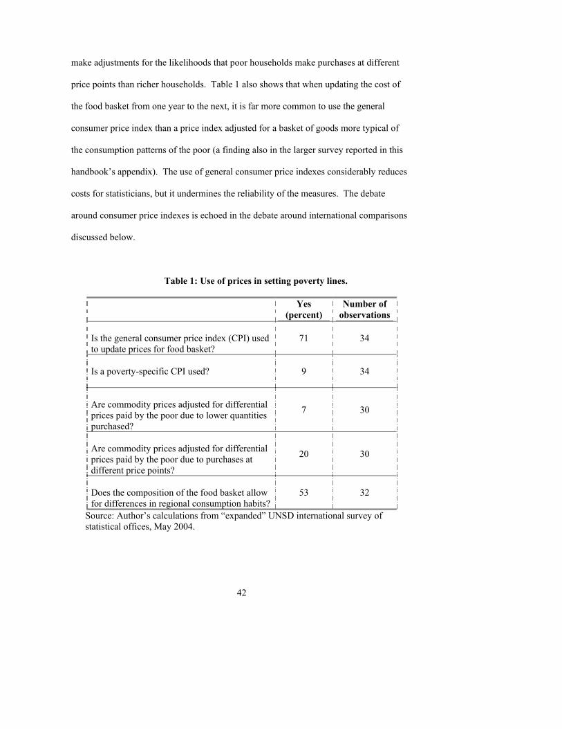
42
make adjustments for the likelihoods that poor households make purchases at different
price points than richer households. Table 1 also shows that when updating the cost of
the food basket from one year to the next, it is far more common to use the general
consumer price index than a price index adjusted for a basket of goods more typical of
the consumption patterns of the poor (a finding also in the larger survey reported in this
handbook�s appendix). The use of general consumer price indexes considerably reduces
costs for statisticians, but it undermines the reliability of the measures. The debate
around consumer price indexes is echoed in the debate around international comparisons
discussed below.
Table 1: Use of prices in setting poverty lines.
Yes (percent)
Number of observations
Is the general consumer price index (CPI) used to update prices for food basket?
71 34
Is a poverty-specific CPI used?
9 34
Are commodity prices adjusted for differential prices paid by the poor due to lower quantities purchased?
7 30
Are commodity prices adjusted for differential prices paid by the poor due to purchases at different price points?
20 30
Does the composition of the food basket allow for differences in regional consumption habits?
53 32
Source: Author�s calculations from �expanded� UNSD international survey of statistical offices, May 2004.
43
Some adjustment for these concerns is implicit in setting separate poverty lines
for urban and rural areas and for different regions. While 46 percent of respondents to
the �expanded� UNSD survey construct only a single poverty line, 25 percent construct
two lines, and 29 percent construct three lines or more. Having multiple lines can add
precision, especially in geographically diverse countries, although it drives costs up.
2.2 International comparisons
It would be helpful to find a way to slash through the multiplicity of possibilities
identified above. One way is to work toward the harmonization of approaches, seeking
methodological consensus across countries. Another is to start from scratch with so-
called international poverty lines.
Poverty measures are used both to compare progress across different countries
(where the need for international comparability is paramount) and within a single country
(where it is possible to customize the approach and definitions). The United Nations and
World Bank have adopted $1/day and $2/day per capita poverty lines for international
comparisons, even though national poverty lines may be more appropriate for
comparisons within a specific country.
44
The UN $1/day line happens to roughly approximate India�s poverty line in the
1980�s.9 The $1/day line was not constructed based on a notion of an international basket
of goods required to achieve basic capabilities, as described by Sen (1987) for example.
Instead, it was chosen as a simple, if arbitrary, threshold that could be used to set goals
and monitor progress. Given the challenge of constructing a consistent poverty line for
any given country, arbitrariness is not surprising when constructing a line meant to apply
globally.
One limit of the international lines is that for richer countries, the $1/day line (or
even the $2/day line) captures few of those considered poor by experts in the countries
themselves. The poverty line in the United States is roughly ten times higher than the
$1/day line, for example. The $1/day poverty line used by the United Nations and World
Bank is anchored in 1993 international prices, so it is instructive to compare the data to
the 1993 poverty line in the United States. In 1993, households in the United States with
two adults and two children were deemed poor if their income fell below $14,654 per
year�or $10.04 per day per person.10 The per-year figure for the US is thus ten times
higher than the international benchmark.
Another limit of the $1/day line involves the translation of the international line
(denominated in US dollars) into country-specific poverty lines (denominated in local
currency). The simplest approach would be to use official exchange rates. But many
9 The poverty line was originally set at $1 per day per person valued at 1985 international prices but was subsequently updated to $1.08 per day in 1993 international prices. The line is still referred to as the $1/day measure, however. 10 See, http://www.census.gov/hhes/poverty/threshld/thresh93.html.
45
goods consumed by the poor are not traded, and official rates can also be distorted by
government interventions. It is thus broadly accepted that official exchange rates cannot
be relied on to give the appropriate conversion of purchasing power when welfare
comparisons are made. These issues have led to a search for alternative methods of
conversion.
The United Nations and World Bank use a set of exchange rates calculated as part
of the International Comparisons Project. These rates are designed to be used for
comparing national income in different countries, and similar to consumer price indices,
these rates are calculated based on the relative prices of a set basket of goods in each
country. The idea is to calculate conversion factors that aim to equalize the purchasing
power of currencies in different countries (which is why they are termed �purchasing
power parity��or PPP--adjustments).
In principle, if a certain kind of man�s shirt costs $10 in the United States, then
$10 converted via the PPP-adjusted exchange rate should allow a person to have exactly
enough money to buy the same shirt in any other country. In practice, the PPP numbers
are difficult to calculate, and corrections and refinements to the method continue. A set
of numbers is available for a large number of countries, however, and the UN and the
World Bank rightly favor them over official exchange rates.
Differences between PPP and official exchange rates are considerable. In late
2003, for example, the ratios of official rates to PPP rates in Brazil, Nigeria, and India
46
were 2.3, 1.4, and 3.3, respectively. This overvaluation of official rates means that the
PPP-adjusted figures raise the value of $1/day poverty lines when denominated in local
currencies�and thus the PPP method shows more poverty in the world than would a
$1/day line translated into local currencies at official exchange rates.
While they are more accurate than official exchange rates, PPP exchange rates
were not originally designed for adjusting poverty lines. In particular, they are not based
on a bundle of goods typically consumed by the poor. Researchers have worried about
(and demonstrated) the potential biases that result from including cars and color
televisions and other goods typically consumed only by richer citizens, and ongoing work
aims to create a set of PPP rates that better reflect the spending patterns of poor
populations.
An alternative approach would be more painstaking but more consistent with the
conceptual basis for poverty measurement described above. The idea would be to focus
on a set of capabilities that people throughout the world can agree are necessary for living
free from the worst deprivations. Elements would likely include having adequate
nutrition, health inputs, shelter, and clothing. Each element would be specified carefully
in the spirit of the �cost of basic needs� approach described above. The components
would be achievable through access to different bundles of goods in different places,
recognizing that eating and living patterns vary considerably the world over. The task for
statisticians would be to construct locally-relevant commodity baskets that reflect the
47
international consensus on these basic capabilities�and to price the baskets using local
costs, avoiding the need to use international exchange rates of any sort.
One advantage of this approach is that region-specific poverty lines could be
easily accommodated, free of reliance on PPP numbers. The project would no doubt
require considerable international coordination and consultation (unlike current practice),
but the reward would be the first truly global poverty approach. Setting new international
poverty lines would be a critical first step.11 As highlighted throughout this handbook,
coordinating survey techniques and practices would be the second major step toward this
ultimate goal.12 For now, though, many countries will continue to rely upon the $1/day
and $2/day per-person poverty lines. They have proved highly effective in focusing
attention on world poverty, and they provide a rough benchmark on global trends. But at
the same time, their limits should be kept in mind, particularly when completing
disaggregated analyses.
2.3 Toward harmonization
A key goal of this handbook is to find common ground in approaches to poverty
measurement, to better understand differences in approaches, and to sharpen assessment
practices overall. While money-based measures no longer have exclusive hold on our
attention, they remain central to analyses. The past two decades of experience, though,
11 Debate around the $1/day poverty line is described in UNDP papers (2004), as well as in Reddy and Pogge (2002), Ravallion (2002), and Deaton (2001). Reddy and Pogge (2002) describe (and advocate) the alternative approach described above. 12 In approaching the second step, there would be much to learn from initiatives like the World Bank�s Living Standards Measurement Survey program and from the Luxembourg Income Studies.
48
reinforce the value of collecting health and education data, as well as other social
indicators that describe broader conditions of poverty. Increasingly, researchers also find
value in asking about subjective views of poverty and in seeking input on poverty
through participatory exercises that involve participants from local communities. Direct
measures of access to basic services and infrastructure also provide important inputs in
the policy�making process.
Results from the 2005 United Nations Statistical Division survey on approaches
to poverty measurement show a wide range of practices. The diversity partly reflects
differences in national conditions and policy needs, but there remain substantial areas
where greater uniformity will raise the overall quality of poverty measure and improve
comparability of measures across time and location. The $1/day poverty line approach
incorporated into the United Nations Millennium Development Goals demonstrates the
power of uniformity, and this chapter points to ways of going further.
Several steps to consider in achieving greater comparability and transparency
include decisions to:
• Base poverty measurement on expenditure data rather than income
data;
• Establish standards for how poverty lines are set, including how to
determine both food and non-food portions of poverty lines (where the
�cost of basic needs� approach is taken);
• Select a standard set of adjustments for adult equivalence;
49
• Select a standard adjustment for economies of scale;
• Create shared guidelines for household survey methods used to collect
important consumption items;
• Create uniform ways of handling missing data and implausibly low
values of income and consumption; and
• Establish guidelines on whether and how to use data from national
income accounts to adjust data from household surveys (many experts
will suggest not doing so at all).
These simple steps, which are discussed further in this handbook, will
bring statistical offices closer toward a common method of measuring
poverty. No set of uniform rules and procedures will be superior for
everyone all the time, but achieving greater uniformity will be a vast
improvement over today�s widely varying practices.
50
References Deaton, Angus (1997). The Analysis of Household Surveys: A microeconometric
approach to development policy. Baltimore: Johns Hopkins.
FAO/WHO/UNU (2004). Human energy requirements - Report of a Joint FAO/WHO/UNU Expert Consultation (17-24 October, 2001). Rome, FAO Food and Nutrition Technical Paper Series, No. 1.
Ravallion, Martin (1994). Poverty Comparisons. Chur, Switzerland: Harwood Academic Press.
Ravallion, Martin (2002). �How Not to Count the Poor: A reply to Reddy and Pogge.�
World Bank working paper. Reddy, Sanjay and Thomas Pogge (2002), �How Not to Count the Poor,� Working paper,
Department of Economics, Barnard College, Columbia University,
Sen, Amartya K. (1987), The Standard of Living. The Tanner Lectures. Cambridge: Cambridge University Press.
Székely, Miguel, Nora Lustig, Martin Cumpa, and José Antonio Mejia (2000). �Do We Know How Much Poverty There Is?� Working Paper #437, Inter-American Development Bank, Washington, DC.
Stedman Jones, Gareth (2004). An End to Poverty: A Historical Debate. London: Profile Books.
United Nations Development Programme (2004), �Dollar a day: How much does it say.�
In Focus, September 2004, International Poverty Centre. Available at: http://www.undp.org/povertycentre/newsletters/infocus4sep04eng.pdf.

51
52
CHAPTER III. POVERTY MEASURES
Jonathan Morduch13
Introduction
This chapter focuses on ways in which statisticians aggregate survey data to
describe the condition of poverty. All governments make poverty reduction part of their
policy agendas, but how exactly should poverty be measured? This chapter takes up that
question with respect to money-based measures: those poverty statistics that measure the
degree to which individuals and households fall below a poverty line.14 Just as there is
much diversity in how surveys are collected, the practice of calculating poverty statistics
also varies widely. The past twenty years have seen a great deal of convergence in
understandings, though, and this chapter draws on what has been learned.
This chapter focuses on ways in which statisticians aggregate survey data to
answer questions such as:
• How many poor people are there in a region?
• How deep is their deprivation?, and
13 I have benefited from the comments of the United Nations Expert Group on Poverty Statistics, and in particular from input from John Gibson, Christian Grootaert, and Branko Milanovic. 14 The poverty line, as described in the previous chapter, is set to reflect the money needed to purchase those goods and services deemed necessary for living a life free of basic deprivation.
53
• Has poverty risen since the last survey?
Any discussion of how to form poverty measures must begin with recognition that
statistics have multiple constituencies (e.g., government policy makers, NGOs,
researchers, and the general public), and these scattered constituencies often have
competing needs and agendas. Choosing which poverty measure is best depends in large
part on the uses to which it will be put. Since no single statistic is likely to answer the
needs of all, most statistical offices publish a range of statistics. Below,
recommendations are made for ways to expand the data range to make comparisons
easier. Even better, although not always easy, would be to also make the raw survey data
available for others to analyze (after taking appropriate actions to protect the
confidentiality of surveyed households).
This chapter begins by describing and comparing four commonly-used poverty
measures. The discussion emphasizes interpretation, and a recently-introduced metric,
�exit time,� which is then defined and illustrated with examples from Bangladesh and
Papua New Guinea. The chapter then moves to a discussion of measurement error and
comparisons based on stochastic dominance that allow researchers to analyze trends in
poverty without using explicit measures. The discussion is framed in terms of income or
consumption deprivation�since this is the form of poverty usually analyzed with the
measures below. But the measures can, in principle, also be used for analyzing other
forms of deprivation when the underlying quantities are measured on a cardinal scale,
54
such as under-nutrition, stunting (height for age), and wasting (weight for height). The
chapter concludes with a set of recommendations on how to improve the measurement of
poverty.
3.1 Desirable features of poverty measures
Poverty measures are used first and foremost to monitor social and economic
conditions and to provide benchmarks of progress or failure. Here, poverty measures are
indicators by which policy results are judged and by which the impact of events (e.g.,
runaway inflation or the introduction of a government transfer program) can be weighed.
Measures used for monitoring and targeting need to be trusted and require rigorous
underpinning. The measures will function well as long as everyone agrees that when
poverty numbers rise, conditions have indeed worsened (and conversely, when poverty
measures fall, that progress has been made). The first question in judging measures is
how well does each index reflect basic properties desirable on philosophical grounds.15
A second important use for poverty measures is descriptive. Poverty statistics
play critical roles in summarizing complex social and economic conditions that inform
conversations around economic and social priorities. For this purpose, effective
measures need not completely capture all (or even most) morally relevant aspects of
poverty. But the limits of measures need to be understood, and transparency and ease of
15 Transparency of method is critical in helping to achieve a consensus, and interested parties should be given enough information to understand exactly how the numbers were constructed, beginning with data collection methods and ending with aggregation techniques.
55
interpretation are critical here. These two notions�the need for rigor balanced against a
desire for ease of interpretation�run through the discussion below.
Economists have sharpened discussions by identifying a set of desirable
normative characteristics of poverty measures (often stated mathematically as axioms)
around which consensus can be built. The search focuses not on identifying descriptively
useful measures in the sense above; instead, the focus is on moral relevance�even if the
outcome is a set of measures that yield numbers with little intuitive meaning.
If we can agree that acceptable poverty measures must satisfy a given set of
axioms or must have certain characteristics, it is possible to sharply narrow the number of
potential candidates for poverty measures. In the most desirable case, a single, unique
measure would emerge that would be fully �characterized��that is, there would be only
one possible candidate that satisfies all of the axioms on which we agree. So far, though,
the search has left a long list of possible poverty measures still on the table, and the task
for analysts remains to understand the basic properties of the chief contenders.
While not succeeding at singling out a particular, universally-acclaimed poverty
measure, the axiomatic approach pushes discussions forward in useful ways, and the
central ideas are worth reviewing. Building blocks include concepts such as �scale
invariance.� This is the idea that poverty measures should be unchanged if, for example,
a population doubles in size while everything else is maintained in the same proportions.
56
A second building block focuses on the well-being of those below the poverty
line�so that changes among better-off people do not affect measured poverty This
�focus axiom� rules out measures based on relative notions of poverty (i.e., where
poverty is not measured by absolute deprivations relative to a fixed poverty line but
instead the poor are identified relative to a shifting statistic like the median income of the
whole population). Our focus here is on �absolute poverty� as measured by a fixed
poverty line.
A third attribute, the �monotonicity� axiom, states that, holding all else constant,
when a poor person�s income falls, poverty measures must rise (or at least should not
fall).
The �transfer� axiom (sometimes referred to as the Pigou-Dalton principle, after
those who employed it first in their analyses) has more analytical bite. It states that,
holding all else constant, taking money from a poor person and giving it to a less poor
person must increase the poverty measure. Conversely, poverty falls when the very poor
gain through a transfer from those less poor.
�Transfer sensitivity,� a related notion, goes further. It is best seen by example.
Consider a population where the poverty line is set at $1,000. Next, imagine that $10 is
taken from someone earning $600 and given to a neighbor earning $500. Any poverty
measure that satisfies the transfer axiom will fall. Measured poverty should also fall (for
such indices) when $10 is taken from someone earning $300 and given to someone
57
earning $200. The transfer-sensitivity axiom says that the reduction in the second case
(in which a very poor person is made better off relative to her neighbor) should be greater
than the reduction in the first case (in which the recipient is less poor).16
An additional desirable characteristic is the ability to decompose poverty
measures by sub-population. Sub-populations may include, for example, residents of
different regions. The critical feature for decomposition is that the sub-groups are
distinct from each other (so that there is no overlap in membership) and that together they
encompass the entire population. All additive indexes are decomposable, and all of the
measures described below share the feature.17
3.2 Four common measures
The simple headcount index is the most used poverty measure, but it violates
several important axioms. Of the four measures described below, the one that satisfies all
of the desirable axioms above--the Watts measure--turns out to be the least used. These
two facts suggest an ongoing tension between the desire for simplicity and transparency
pitched against the desire for rigor. The measures below will be compared in that light.
All of the measures will be described in terms of shortfalls of �income.� The
focus on income keeps discussion simple, but the measures may instead may be used to
gauge shortfalls in consumption and spending�following the discussion in Chapter 1. 16 For a broader discussion of axioms, see Sen (1976), Foster (1984), and Foster, Greer, and Thorbecke (1984). 17 Decomposability is the focus of Foster, Greer, and Thorbecke (1984).
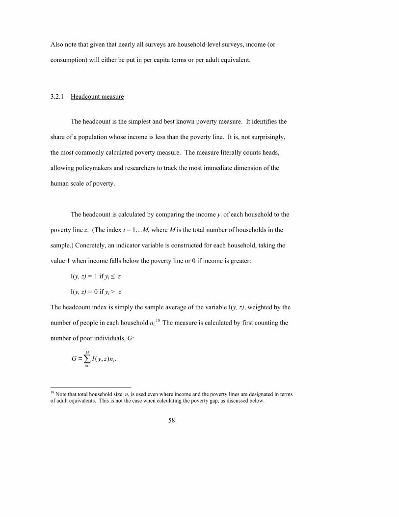
58
Also note that given that nearly all surveys are household-level surveys, income (or
consumption) will either be put in per capita terms or per adult equivalent.
3.2.1 Headcount measure
The headcount is the simplest and best known poverty measure. It identifies the
share of a population whose income is less than the poverty line. It is, not surprisingly,
the most commonly calculated poverty measure. The measure literally counts heads,
allowing policymakers and researchers to track the most immediate dimension of the
human scale of poverty.
The headcount is calculated by comparing the income yi of each household to the
poverty line z. (The index i = 1�M, where M is the total number of households in the
sample.) Concretely, an indicator variable is constructed for each household, taking the
value 1 when income falls below the poverty line or 0 if income is greater:
I(y, z) = 1 if yi ≤ z
I(y, z) = 0 if yi > z
The headcount index is simply the sample average of the variable I(y, z), weighted by the
number of people in each household ni.18
The measure is calculated by first counting the
number of poor individuals, G:
∑=
=M
iinzyIG
1.),(
18 Note that total household size, n, is used even where income and the poverty lines are designated in terms of adult equivalents. This is not the case when calculating the poverty gap, as discussed below.
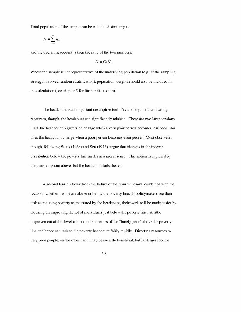
59
Total population of the sample can be calculated similarly as
∑=
=M
iinN
1,
and the overall headcount is then the ratio of the two numbers:
.NGH =
Where the sample is not representative of the underlying population (e.g., if the sampling
strategy involved random stratification), population weights should also be included in
the calculation (see chapter 5 for further discussion).
The headcount is an important descriptive tool. As a sole guide to allocating
resources, though, the headcount can significantly mislead. There are two large tensions.
First, the headcount registers no change when a very poor person becomes less poor. Nor
does the headcount change when a poor person becomes even poorer. Most observers,
though, following Watts (1968) and Sen (1976), argue that changes in the income
distribution below the poverty line matter in a moral sense. This notion is captured by
the transfer axiom above, but the headcount fails the test.
A second tension flows from the failure of the transfer axiom, combined with the
focus on whether people are above or below the poverty line. If policymakers see their
task as reducing poverty as measured by the headcount, their work will be made easier by
focusing on improving the lot of individuals just below the poverty line. A little
improvement at this level can raise the incomes of the �barely poor� above the poverty
line and hence can reduce the poverty headcount fairly rapidly. Directing resources to
very poor people, on the other hand, may be socially beneficial, but far larger income
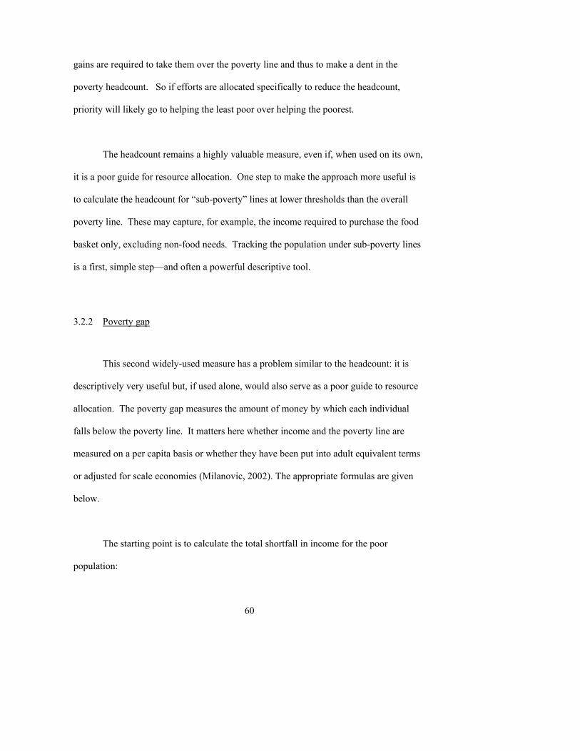
60
gains are required to take them over the poverty line and thus to make a dent in the
poverty headcount. So if efforts are allocated specifically to reduce the headcount,
priority will likely go to helping the least poor over helping the poorest.
The headcount remains a highly valuable measure, even if, when used on its own,
it is a poor guide for resource allocation. One step to make the approach more useful is
to calculate the headcount for �sub-poverty� lines at lower thresholds than the overall
poverty line. These may capture, for example, the income required to purchase the food
basket only, excluding non-food needs. Tracking the population under sub-poverty lines
is a first, simple step�and often a powerful descriptive tool.
3.2.2 Poverty gap
This second widely-used measure has a problem similar to the headcount: it is
descriptively very useful but, if used alone, would also serve as a poor guide to resource
allocation. The poverty gap measures the amount of money by which each individual
falls below the poverty line. It matters here whether income and the poverty line are
measured on a per capita basis or whether they have been put into adult equivalent terms
or adjusted for scale economies (Milanovic, 2002). The appropriate formulas are given
below.
The starting point is to calculate the total shortfall in income for the poor
population:
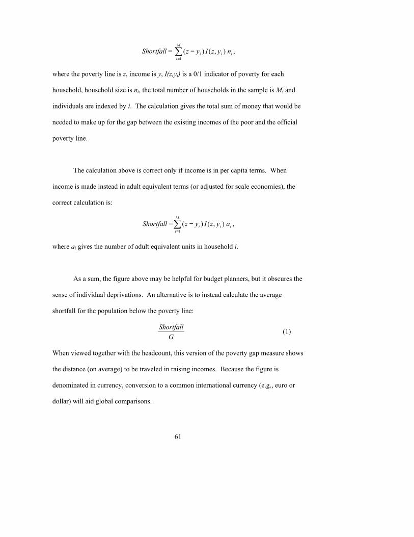
61
Shortfall = ii
M
ii nyzIyz ),()(
1∑
=
− ,
where the poverty line is z, income is y, I(z,yi) is a 0/1 indicator of poverty for each
household, household size is ni, the total number of households in the sample is M, and
individuals are indexed by i. The calculation gives the total sum of money that would be
needed to make up for the gap between the existing incomes of the poor and the official
poverty line.
The calculation above is correct only if income is in per capita terms. When
income is made instead in adult equivalent terms (or adjusted for scale economies), the
correct calculation is:
Shortfall = ii
M
ii ayzIyz ),()(
1∑
=
− ,
where ai gives the number of adult equivalent units in household i.
As a sum, the figure above may be helpful for budget planners, but it obscures the
sense of individual deprivations. An alternative is to instead calculate the average
shortfall for the population below the poverty line:
GShortfall
(1)
When viewed together with the headcount, this version of the poverty gap measure shows
the distance (on average) to be traveled in raising incomes. Because the figure is
denominated in currency, conversion to a common international currency (e.g., euro or
dollar) will aid global comparisons.
62
A different approach that can enhance comparability is to divide the index by the
poverty line:
Gz
Shortfall (2)
Normalization puts the average gap in terms of the percentage shortfall from the poverty
threshold, freeing the measure from denomination in a particular currency. The measure
is now easily comparable across countries and across time, a helpful improvement.
Routinely publishing poverty lines alongside the normalized poverty gap and the
headcount would allow observers to calculate for themselves all three of the poverty gap
variations described above.
The three data points (headcount, poverty gap, and poverty line) can be combined
to form another widely-used variant of the poverty gap:
NzShortfall (3)
Here, the resource shortfall is divided by the total population, rather than the population
of the poor. The measure is often misinterpreted as giving the average income shortfall
of the poor, but that is only the case for versions (1) or (2). Dividing by the total
population sacrifices simple interpretations�the measure no longer gives a quick sense
of deprivation of poor individuals since data on non-poor people are also included. The
measure points up tensions between descriptively-useful measures and measures that can
best serve as guides for monitoring and targeting.
63
The measure in (3) does, though, avoid a common problem with variants (1) or
(2). Specifically, the poverty gap in (1) and (2) can rise�rather than fall�when
individuals exit poverty. This occurs when the least poor are the ones who move above
the poverty threshold (which is the typical pattern). Holding all else the same, those who
exit poverty leave behind a population that is then smaller and, on average, poorer than
before. Conditions would thus seem to worsen when someone exits poverty--if seen
through the lens of the poverty gap as calculated following (1) or (2)--when in fact
conditions have improved overall. The measure in (3) instead captures improvement due
to the exit. The problem here occurs when the poverty gap in (1) or (2) is used as a sole
indicator of progress; it performs poorly when people cross the poverty line.
Version (3) does not have that problem. But as noted, it lacks a simple
interpretation and, along with all of the versions above, it fails to satisfy the transfer
axiom. This failure follows from neutrality with regard to whose income goes up and
down among the poor population. For the transfer axiom to be satisfied, it is not enough
to be neutral: it must be that gains for the poorest are weighed more heavily than gains
for the less poor. Even in version (3), no accommodation is made to weigh progress in
reducing extreme poverty differently from progress in reducing moderate poverty.
In summary, version (2) can be useful as a descriptive tool, especially alongside
other measures. Version (3) has some desirable properties from an analytical vantage.
But as discussed below in sections 3.2.3 and 3.2.4, distributionally-sensitive measures do
even better. Version (3) has gained favor by being a member of the Foster-Greer-
64
Thorbecke class of measures described below (specifically, the case in which α = 1). But
the attention seems misplaced. If a single poverty measure is required, version (3) of the
poverty gap has less appeal than the measures described in sections 3.2.3 and 3.2.4--
although it would be preferred over having, say, version (2) on its own.
All of this is rhetorical since it is seldom that only one poverty measure is
calculated. When multiple poverty measures are produced and published simultaneously
(say, the headcount and a few others), version (2) of the poverty gap stands as a useful
part of a collection. Version (2) features a clear, simple interpretation that is relevant for
policy discussions, an attribute lacking in version (3). A recommended set of basic
poverty indicators would thus include the headcount, version (2) of the poverty gap, the
median income of the poor, and the squared poverty gap described in section 3.2.4.
3.2.3 Watts index
A simple poverty measure that satisfies the transfer axiom was first put forward
by Watts (1968), who argued for the following measure:
[ ] .),()ln()ln(11∑
=
−M
iiii nyzIyz
N (4)
As above, when income is calculated in adult equivalent terms, the household size
variable ni should be replaced with the adult equivalent size ai. The measure is
65
�distributionally-sensitive� by virtue of its use of logarithms.19 The way that the
logarithm is used means that the Watts index is much more sensitive to changes in the
lowest incomes than it is to changes for those with higher incomes. That is, transferring
$10 to a very poor person counts as a far larger contribution to poverty reduction than
transferring $10 to a richer (but still poor) neighbor.
Allocating anti-poverty resources to minimize the Watts index would thus tilt
efforts toward the poorest�which is a feature that many analysts find appealing (and one
also featured by the squared poverty gap and the influential (but seldom applied) measure
of Sen, 1976). The Watts index also satisfies the transfer-sensitivity axiom described
above, and it is decomposable into the population-weighted sum of the poverty indices of
regions or groups. (The squared poverty gap of section 3.2.4 shares this feature too.)
Being decomposable is useful when a population can be divided into a number of distinct
groups or regions. Poverty measures can then be calculated for each group or region,
and, if the poverty measure is decomposable, the individual poverty measures can be
aggregated (using population shares as weights) to form the overall poverty measure for
the entire population. Decomposing poverty measures in this way can help to pinpoint
the groups or regions contributing most�and least--to overall poverty.
Given these appealing features, the Watts index can be a useful measure, and we
return to it below in comparison to the �squared poverty gap� and the �average exit time�
measures (see sections 3.2.4, 3.3, and 3.4). The comparisons in section 3.3 show that an
19 If a given number is larger than another, then the logarithm of the first will also be larger than the logarithm of the second. But the logarithmic transformation is nonlinear, i.e., the ratio of the two numbers will be larger than the ratio of their logarithms.
66
important difficulty with the Watts index is that the weights on money in the hands of the
�least poor� and the �moderately poor� are quite close, while the weights on the �most
poor� and destitute are particularly heavy. As section 3.3 shows, the �squared poverty
gap,� in contrast, leads to greater differentiation across the entire distribution of incomes
below the poverty line and may be preferable for that reason.
3.2.4 Squared poverty gap
One way to transform the poverty gap described above into a distributionally-
sensitive measure is to raise the individual gaps to a power greater than 1. Foster, Greer,
and Thorbecke (1984; henceforth, FGT) propose a class of measures built on this idea
which have found their way into much of the poverty analysis published by the World
Bank. With income expressed in per capita terms, the measures take the form:
( )
.),(11∑
=
−M
iii
i nyzIz
yzN
α
(5)
When income is in adult-equivalent terms, the household size variable ni should be
replaced with the adult equivalent size ai.
The parameter α determines the degree to which the measure is sensitive to the
degree of deprivation for those below the poverty line. When α is zero, the measure
collapses to the headcount measure described above, and when α is one, the measure is
the normalized version of the poverty gap (equation 3 above). In neither case is the
measure distributionally-sensitive. But for α > 1, the measure is distributionally
67
sensitive. And the particular case in which α = 2 (often referred to as the squared poverty
gap) is now the most widely-used distributionally-sensitive measure.
By squaring the poverty gap, improvements in the resources of the poorest
individuals count most, since they are the ones for whom the initial resource gap is
largest. The measure satisfies the transfer axiom but not the transfer-sensitivity axiom.
To satisfy the latter, the poverty gap would have to be raised to a higher power�cubed
rather than squared, say. Cubing adds �transfer sensitivity,� a property that many find
appealing. But it puts very heavy weight on the well-being of the poorest�perhaps
weight that would be judged too great in a social calculus.20 At levels of α between 1 and
2, not only is transfer sensitivity not satisfied but the reverse holds: holding all else the
same, a regressive transfer among the very poor increases poverty less than a same-sized
regressive transfer among the moderately poor�a clearly undesirable feature.
Distributional-sensitivity is achieved by weighing deprivations of the poor
inversely to their base incomes. There are many ways to do this, and the weighting
scheme in the squared poverty gap has the advantage of relative simplicity. The
simplicity can help provide some intuition in understanding why the poverty measure
moves over time. This is described below in the context of Figure 1.
3.3 Comparing the measures
20 Transfer sensitivity is obtained through setting α at any level larger than 2 (2.2, for example), but analyses have focused on integer values.
68
Neither the Watts index, nor the squared poverty gap, nor the cubed poverty gap
yield particularly easy-to-interpret numbers. As noted above, we rely for interpretation
on our knowledge that the indices satisfy (or do not satisfy) certain axioms, notably the
transfer axiom and transfer-sensitivity axioms. Often that is enough, and at times each of
the three indexes will rank income distributions identically. So the form of the poverty
index may not matter when answering relevant policy questions. In other cases, though,
results will depend on the choice of index, and the relatively opaque nature of the indexes
hides the fact that even indexes with similar basic properties (e.g., Watts and the cubed
gap) weigh income gains very differently for different people.
Figure 1 makes this explicit. The question asked in the figure is: how does giving
$1 to a person with income equivalent to, say, 50 percent of the poverty line compare to
giving the $1 to someone with income equivalent to 90 percent of the poverty line?
Specifically, how does the transfer contribute to measured poverty?
The figure shows how the answer depends on the choice of poverty measure. It
demonstrates the relative weight of a $1 increase in income as implied by the four
measures above�the poverty gap (equation 3 above), squared poverty gap, cubed
poverty gap, and the Watts index. The horizontal axis gives a poor person�s income
relative to the poverty line, from 0 percent at the left to 100 percent at the right. Those on
the far right are just at the poverty line (which was set at $100 for this illustration). The
$1 increases are depicted relative to a $1 increase for a person whose income is at 90
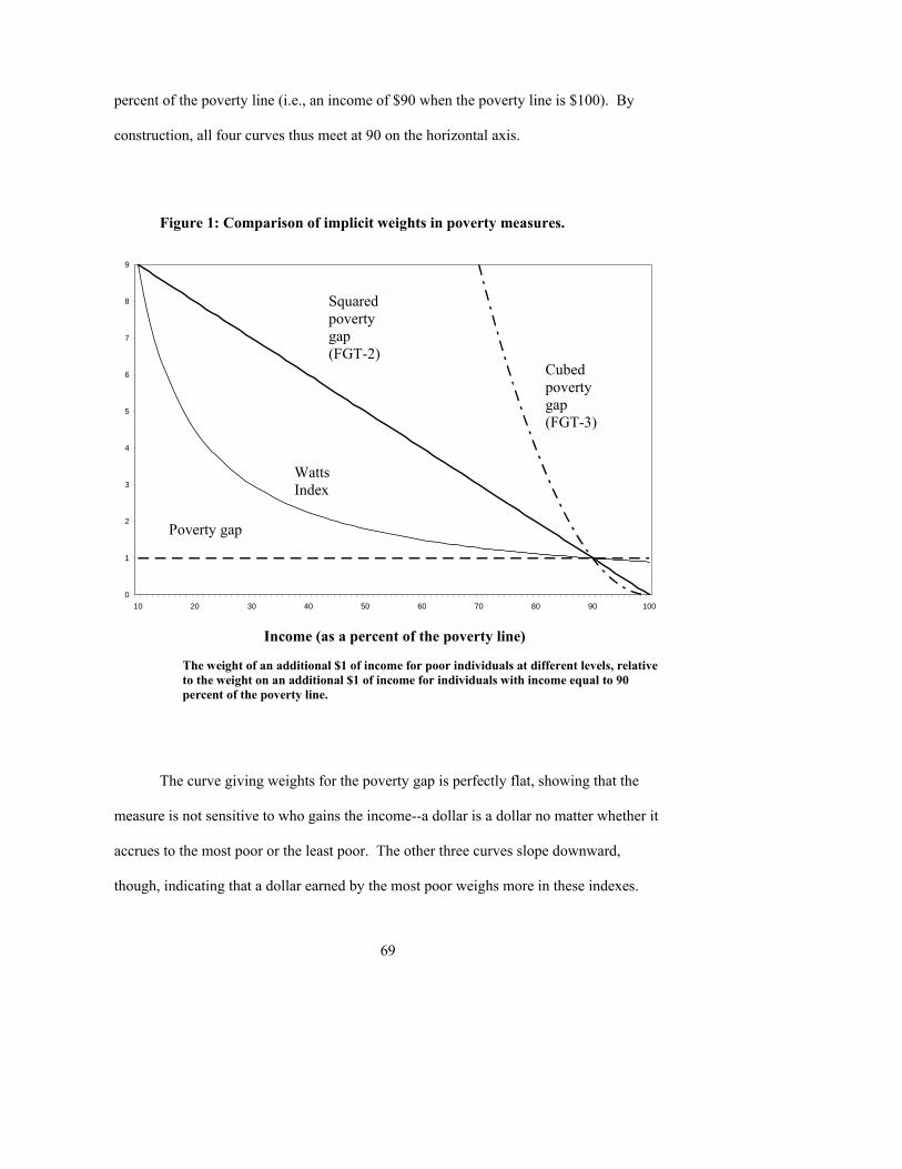
69
percent of the poverty line (i.e., an income of $90 when the poverty line is $100). By
construction, all four curves thus meet at 90 on the horizontal axis.
Figure 1: Comparison of implicit weights in poverty measures.
0
1
2
3
4
5
6
7
8
9
10 20 30 40 50 60 70 80 90 100
The weight of an additional $1 of income for poor individuals at different levels, relative to the weight on an additional $1 of income for individuals with income equal to 90 percent of the poverty line.
The curve giving weights for the poverty gap is perfectly flat, showing that the
measure is not sensitive to who gains the income--a dollar is a dollar no matter whether it
accrues to the most poor or the least poor. The other three curves slope downward,
though, indicating that a dollar earned by the most poor weighs more in these indexes.
Squared poverty gap (FGT-2)
Cubed poverty gap (FGT-3)
Watts Index
Poverty gap
Income (as a percent of the poverty line)
70
The curve for the cubed-poverty gap arcs so sharply that it goes off the graph. Giving $1
to a person weighs 9 times more if the recipient has income of $70 than if the recipient
starts with income of $90 (relative to a poverty line of $100). The weighting is thus
heavily skewed to the very poor � and certainly far more skewed than is the case for the
squared poverty gap.
For the squared poverty gap, the ratio of weights is proportional to base income.
For example, a dollar accruing to someone with income of $70 (i.e., 30 percent below the
line) is 3. At $80 (i.e., 20 percent below the line), the ratio is 2. And so forth. This
property would be highlighted if the measure were renamed the �gap-weighted� index,
say, since the income gap for each household (i.e., z - yi) is weighted by the size of the
income gap itself (which is, again, z - yi).
The Watts index takes a very different form, weighing increases from very low
incomes very heavily, but staying flatter for less poor individuals. The ratio in the figure
only hits 2 when the added dollar accrues to individuals whose incomes are below $50.
The relative weights, as seen by the ratio in the figure, are always below those of the
squared gap, except for transfers made to people with incomes below $10. At that level,
income is so low that (it is hoped) few if any people could survive at those levels. The
weighting scheme corresponds with moral concerns that focus on the very, very poorest
with extreme intensity, in contrast to the squared poverty gap which has a linear profile of
relative weights. On the other hand, the Watts index exacerbates bias due to
71
measurement error if the reported incomes at the very low end are largely the result of
poor data collection and mis-reporting.
None of the weighting schemes can claim universal preference from a normative
stance, but the square poverty gap is a middle ground, and this likely explains much of its
continuing appeal. The Watts index, though should not be altogether dismissed. It has a
useful feature through its association with the exit-time concept and value as a descriptive
tool.
3.4 Exit time and the value of descriptive tools
For all of the theoretical appeal of the distributionally-sensitive measures
described immediately above, the headcount remains�by far�the most common
poverty measure in use. The Millennium Development Goals, for example, focus on
reducing the headcount of poverty below $1/day, rather than minimizing a
distributionally-sensitive measure.
One reason for the continuing use (and usefulness) of the headcount is its
descriptive properties. It is a simple means for illustrating the scale of poverty. In this
sense, it is an intrinsically meaningful measure.
The poverty gap is also intrinsically meaningful, taking us from counting people
to counting shortfalls of income or consumption. It answers the question: how much
72
would have to be spent to eliminate poverty through costless (and perfectly) targeted
transfers. Its underlying assumptions are clearly unrealistic: in practice, transfers will
never be administratively costless, nor will they ever be perfectly targeted. However, this
hypothetical question still provides a helpful way to quickly gauge the scale of
deprivation.
The �average exit time,� introduced in Morduch (1998), is based on a similar sort
of hypothetical question. The underlying assumption is as unrealistic as that under the
poverty gap, but the measure nevertheless can fruitfully frame discussions of poverty.
The measure is based around the number of years that it would take poor households to
grow out of poverty given a hypothetical, steady growth of income. (An equivalent
question could also be asked about consumption growth, rather than income.)
In practice, income growth will seldom be steady over long periods, nor will all
poor households be able to grow at the same rate. But, as with the poverty gap, asking the
hypothetical question provides a quick way to gauge one important aspect of the
condition of poverty.
Hypothetical exit times are simple to calculate. If the assumed growth rate of
income is g percent per year, an individual whose income starts at yi will take T years to
exit, where T solves this equation:
Ti gyz )1( += (6)
73
The equation can be solved by taking logarithms, yielding that the number of
periods of growth required before exit is T = ln(z/yi) / g. Of course, T = 0 for all
households already above the poverty line. So, for example, if a person�s income starts at
80 percent of the poverty line and his income grows at 5 percent per year (after adjusting
for inflation), his exit time will be ln(100/80) / 0.05 = 4.5 years.
The calculation shows that within five years, consistent, broad-based income
growth of 5 percent would be enough to push from poverty everyone whose income is 80
percent of the poverty line or higher. Exit times based on this calculation are shown in
Figure 2, based on assumed growth rates of 3 percent, 5 percent, and 10 percent.
Alternatively, a figure could be constructed that fixes the hypothetical growth rate and
maps a profile of exit times for the entire poor population, with exit times shown
according to the fraction of the population at each level of income below the poverty line.
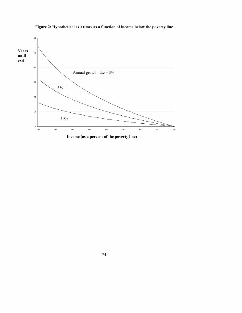
74
Figure 2: Hypothetical exit times as a function of income below the poverty line
0
10
20
30
40
50
60
20 30 40 50 60 70 80 90 100
Annual growth rate = 3%
5%
10%
Income (as a percent of the poverty line)
Years until exit
75
In a related calculation, Morduch (2000) focuses on the �median exit time� when
illustrating the use of exit times with data from Bangladesh. The calculation is simple:
ln(z/yM)/g. The only data required are the poverty line z, the assumed growth rate g, and
the median income of the population below the poverty line yM. The median poor rural
household in the 1988-89 Household Expenditure Survey spent Taka 284 per month per
capita relative to the poverty line of Taka 370. (In 1989, Taka 32.1 = $1.) So, if median
expenditures grew steadily at 3 percent per year, it would take just under 9 years to
reduce half of rural poverty through growth alone�ln(370/284)/.03.
If the hypothetical exit time , Ti, for each poor household is averaged over the
population below the poverty line, the �average exit time� is:
∑∑==
==M
iii
M
iii
i nTG
nyzIg
yzG
A11
1),()/ln(1 (7)
This equation is analogous to the average poverty gap described in equation (2), and it
shares similar weaknesses and strengths. Its chief strength is its simplicity and
descriptive value. Its main weakness is that when a less poor household exits poverty and
all else is unchanged, the average exit time, A, will fall. This makes A a poor candidate to
be the sole measure of poverty. However, A can still be a very useful component of the
analyst�s toolkit.
76
One aspect that makes the average exit time potentially valuable is that it can be
decomposed explicitly to show the impact of inequality below the poverty line. Start
with the average income of households below the poverty income:
.),(11∑
=
=M
iiii
avg nyzIyG
y
If everyone below the poverty line had exactly this income (i.e., there was no inequality
below the poverty line), then this hypothetical average exit time would be:
./)/ln( gyzT avgavg =
Using these relationships, the average exit time of the poor population (A in equation 7
above) can be rewritten simply as:
A= ,/ gLT avg + (8)
where L is the Theil-L measure of inequality--a commonly used inequality index. The
decomposition shows the explicit contribution of income inequality to the average exit
time.
In their survey of 1,144 households in Papua New Guinea, Gibson and Olivia
(2002) found that given an assumed, hypothetical growth rate of 2 percent per year, the
average exit time of the population would be 20.5 years. Their calculation helps to frame
the potential importance of growth-based strategies�if growth is steady and broad. They
decompose the result to show that the exit time of a person with income equal to the
average income of the poor population (i.e., Tavg) is 17.8 years, so the explicit impact of
inequality below the poverty line is an increase in the average exit time by 2.7 years.
77
The exit time has a useful relationship to another established measure. If exit
times are calculated for the entire population of a country (with those above the poverty
line having 0 exit times), the average turns out to be simply the Watts poverty index
divided by g, the hypothetical annual growth rate.21 This measure, the �population
average exit time,� naturally shares all properties of the Watts index, satisfying both the
transfer axiom and the transfer-sensitivity axiom. But it has the addition of a new
interpretation, akin to the interpretation of the poverty gap described by equation (3)
above.
With economic growth very much a part of the poverty reduction policy agenda,
tools like exit times provide ways to summarize data in a manner relevant to policy
debates on growth-based poverty strategies. They complement the other measures
described above, rather than substituting for measures whose appeal rests primarily on
their axiomatic properties. By the same token, those theoretically-appealing measures
cannot substitute for simpler tools that provide new ways of describing the data and
identifying trends. And, importantly, it should be remembered that exit times describe
possibilities based on simple assumptions�as used here, the exit times are not based on
actual forecasts or careful predictions. These simple exit times, though, can be useful in
identifying opportunities and constraints to guide policy.
21 This measure satisfies the monotonicity transfer, and transfer-sensitivity axioms. As a result of its additively separable form, the measure is also decomposable into the population-weighted measures of sub-populations of the poor.
78
3.5 Broader concerns
3.5.1 Comparisons without poverty measures
For many purposes, the relevant policy question is simply: is poverty larger or
smaller in one survey versus another? As noted above, the answer can depend on which
poverty line and which measure is used in the analysis. But that is not always so. It may
be that one survey finds a greater fraction of the population exists at every income level
below the poverty line, relative to the fractions of the population reported by another
survey.
When that is so, the first survey can be said to �stochastically dominate� the latter
(Ravallion, 1994), and conclusions about poverty rates can be made irrespective of
whether the poverty line is moved lower or whether the poverty measure chosen is the
Watts index, headcount, or one of the poverty gap measures described in section 3.3.
Formally, the condition for �first order� stochastic dominance is that with regard to two
samples, A and B, if the cumulative distribution function of their income distributions is
such that DA(y) < DB(y) for all incomes y below the poverty line, then sample A
stochastically dominates sample B.
When income distributions cross below the poverty line (i.e., when DA(y) < DB(y)
in some income range but DA(y) > DB(y) in another), more restrictive notions of
stochastic dominance can be applied which, nonetheless, allow broad statements that are
79
robust to a wide range of choices of poverty lines or measures. These approaches�
�second order� and �third order� stochastic dominance--are described further by
Ravallion (1994). When these robust approaches can be employed, questions about the
choice of method can be avoided. Their disadvantage is that they only answer a simple
question�is poverty higher or lower in sample A than B? Richer descriptive tools (like
the hypothetical exit times discussed above) are required to inform richer policy
questions.
3.5.2 Measurement error
The chapters that follow in the handbook focus largely on methods for collecting
surveys. No survey is perfect, but some collection methods are far more reliable than
others. Particular problems arise when expenditures (or incomes) are either substantially
over-counted or under-counted, and the biases can be exacerbated by the choice of
poverty measure. Under-counting leads to exaggerations of poverty rates, and the
distributionally-sensitive measures described here are particularly susceptible to the
exaggeration of under-counting in the lower tail of the income distribution.
Figure 1 (above), which shows the implicit weights in several popular poverty
measures, also helps to illustrate the potential problems of under-counting. The figure
shows the weight given to an extra $1 of income for households at different levels of base
income, relative to the weight of an extra $1 for an individual whose income is 10 percent
below the poverty line. The figure also can be interpreted as giving the weights of $1 of
80
mis-measured income for different individuals. Clearly, for distributionally-sensitive
measures, every dollar that is mis-measured at the low end of the distribution has a far
larger impact on poverty than a dollar mis-measured closer to the poverty line.
The pattern of weights can mean that mis-measurement in just a small fraction of
observations can make a large difference to results if it takes the form of severe under-
counting. Many household surveys, for example, include responses from some
households about spending and income patterns that, for one reason or another, are
implausibly close to zero. If those observations are taken at face value, they can translate
into large movements in poverty measures.
When using the Watts index, for example, adding an extra dollar for someone
with measured income that is extremely low�say, their total income is no more than 5
percent of the poverty line (a level so low that long-term survival is hard to imagine if
income is measured correctly and savings are unavailable)--would lead to a change in the
index which is 18 times the weight of the dollar for someone with income at 90 percent
of the poverty line. (This result is so extreme that it cannot be seen in Figure 1.) When
using the squared poverty gap, the relative weight would be 9.5 times. It is unclear from
a moral standpoint which is the �correct� weight, but in choosing a poverty measure
analysts are implicitly making a choice, and it should be borne in mind. In making that
choice, it matters greatly whether one believes that very low incomes are most likely a
function of measurement error or whether they reflect actual conditions. Fortunately,
there are very few observations in these data ranges, but the weighting accentuates their
importance.
81
The best solution is to maintain high-quality data and to be especially vigilant
about potential measurement error at the low end. The following chapters, especially
Chapter 5, provide guidance on this matter. But where the quality of data is uncertain, it
is important to remain alert to prevent the choice of measure that could worsen quality
problems. Robustness checks become all the more helpful.
3.6 Conclusions
There is now an extensive literature on poverty measures, and statistical offices have
a wide range of numbers to analyze. Focusing on the most commonly used measures
promotes comparability across countries. These include the headcount index, poverty
gap, and squared poverty gap. This chapter describes how to calculate and interpret these
measures (in addition to the Watts index), and identifies their respective strengths and
weaknesses.
When multiple poverty measures are produced and published simultaneously (say,
the headcount and a few others), a recommended set of basic poverty indicators includes
the headcount in section 3.2.1, version (2) of the poverty gap in section 3.2.2, and the
squared poverty gap described in section 3.2.4.
Statistical offices can go further, though, by also publishing simple statistics that
provide a richer picture of conditions. These statistics are seldom very costly to compute
82
and can substantially enrich analysis. The first is the median income of the poor
population. The median gives the income level below which the bottom 50 percent of the
poor population lives. This simple measure indicates whether the bulk of the poor
population is close to or far away from the poverty line. In section 3.5 above, it was also
shown how median income can be employed in the exit-time framework.
Going further, it would be helpful to also publish the income of households at the
25th percentile and the 75th percentile of the income distribution below the poverty line.
Ultimately, publishing the entire Lorenz curve (the mapping of population shares to
income shares) would be most revealing and would add little extra cost. The median,
though, is the natural place to start, followed by incomes at other important focal points
of the distribution.
The move toward publishing headcounts of the number of people below a
�hardcore� poverty line has accelerated. This is a useful step from a descriptive vantage,
although there is currently little consensus on how to define hardcore poverty.
The exit-time framework was introduced in section 3.4 as an example of a simple
metric that can help policy makers debate ways to promote economic growth and
alleviate poverty. It is a descriptive device based on an unrealistic, best-case scenario. It
asks: how quickly would households exit poverty if their incomes grew at a given, fixed
rate each year? While hypothetical, the answers integrate the notion of time into poverty
programs. The exit time is put forward as a complement to the poverty-gap measure of
83
section 3.2.2, which is built on a similarly unrealistic hypothetical policy scenario, but
which nonetheless offers useful insights.
Over time, new measures and approaches will continue to emerge. One of the
most valuable steps that statistical offices can take is to put in place ways to make the raw
data for poverty analyses available to researchers. Steps would have to be taken to secure
confidentiality to households in the survey, but fortunately methods to do so are now
well-established. Broadening access to data will allow analysts to better compare
conditions and to develop new tools that can ultimately benefit statistical offices, policy
makers, and citizens.
84
References Foster, James (1984), �On Economic Poverty: A Survey of Aggregate Measures,�
Advances in Econometrics 3, 215 - 251. Foster, James, Joel Greer and Erik Thorbecke (1984), �A Class of Decomposable Poverty
Measures.� Econometrica 52, May: 761-766. Gibson, John and Susan Olivia (2002). Attacking Poverty in Papua Guinea, But for How
long?� Pacific Economic Bulletin 17 (2). Kanbur, Ravi (1987), �Measurement and Alleviation of Poverty, with an Application to
the Effects of Macroeconomic Adjustment,� IMF Staff Papers 34(1), March, 60 -- 85.
Milanovic, Branko (2002). �Do We Tend to Overestimate Poverty Gaps? The Impact of Equivalency Scales on the Calculation of the Poverty Gap.� Applied Economics Letters 2002 (9): 69-72.
Morduch, Jonathan (1998). �Growth, Poverty, and Average Exit Time,� Economics
Letters 58: 385 - 390. Morduch, Jonathan (2000). �Reforming Poverty Alleviation Policies,� in Anne Krueger,
ed., Economic Policy Reform: The Second Stage. Chicago: University of Chicago Press, 2000.
Ravallion, Martin (1994). Poverty Comparisons. Chur, Switzerland: Harwood Academic
Press. Ravallion, Martin (2002). �How Not to Count the Poor: A reply to Reddy and Pogge.�
World Bank working paper. Sen, Amartya (1976), �Poverty: An Ordinal Approach to Measurement,� Econometrica
44: 219- 231. Sen, Amartya K. (1987), The Standard of Living. The Tanner Lectures. Cambridge:
Cambridge University Press. Watts, Harold (1968), �An Economic Definition of Poverty,� in On Understanding
Poverty, ed. by Daniel Patrick Moynihan. New York: Basic Books.
85
CHAPTER IV. COUNTRY PRACTICES IN COMPILING POVERTY STATISTICS
Isidoro P. David
Introduction
This chapter provides a review of the poverty measurement practices in member
countries of the United Nations. It is found that the large majority of developing countries
follow the Cost of Basic Needs (CBN) approach in producing income or expenditure-
based poverty statistics. The chapter thus concentrates on absolute poverty measures and
glosses over others more popularly used metrics in developed countries, such as relative
and subjective poverty measures. Practical difficulties confronted by National Statistical
Offices (NSO�s) in implementing the CBN method are discussed and analyzed
systematically and alternative ways of solving some of these difficulties are proposed.
Absolute poverty measures are discussed in Section 4.1. Direct measures of food
poverty which lead to more reliable and comparable estimates are presented in Section
4.2. Non-income measures, particularly minimum basic needs or unmet basic needs
indicators, are dealt with briefly in Section 4.3. This chapter concludes with Section 4.4,
which discusses the main causes of disharmony in countries� poverty monitoring
programs and the sources of non-comparability of their poverty statistics. It then offers
recommendations for improvement.
86
4.1 Income- or expenditures-based measurement approaches
The four UNSD sub-regional workshops on poverty statistics (described in
Chapter 1) confirmed that the majority of the developing countries that compile poverty
statistics follow the CBN approach or some variation of it. In this approach, everyone�s
basic needs may be thought of as falling into two categories--food and non-food.
Broadly, the CBN approach involves a three-step assessment:
• Define the minimum nutritional requirements of a poor person and determine a food
basket or bundle that can provide this minimum requirement. The cost of buying the
food bundle is a food poverty line ( fpl ).
• Choose an operational definition of a poor person�s basic non-food needs that will
allow estimating their cost directly or indirectly. Use this non-food basic needs cost to
adjust fpl upward into a total poverty line ( tpl ).
• Compare fpl and tpl against some metric, e.g. distribution of income or expenditure
per person. The proportion of persons whose incomes (expenditures) fall below fpl
is an estimate of food poverty incidence. Some countries refer to this also as core
poverty incidence or extreme poverty incidence. The proportion of persons whose
incomes (expenditures) fall below tpl is an estimate of absolute poverty incidence.
The same procedure is followed to estimate the number of food poor or absolutely
poor persons. In addition to persons, countries also routinely produce poverty
estimates in terms of households.
87
Some countries follow more than one approach and produce multiple sets of
poverty statistics. However, in the remainder of this section, the CBN approach, as
practiced in many developing countries, will be discussed more thoroughly. Possibilities
for harmonization and sources of non-comparability will be highlighted. Ways for
improving comparability will also be delineated.
4.1.1 Specify a food poverty threshold National food poverty lines are based on minimum nutritional requirements or
thresholds. A person is counted as �food poor� if the nutritional content of the food(s) he
consumes is less than the prescribed threshold. As a simplifying assumption, most
countries use dietary energy as a proxy for overall nutritional status, i.e., if a person gets
enough energy, then she also gets adequate protein and the other essential nutrients.
Countries are guided by FAO/WHO recommended daily allowance (RDA) for
energy, defined as �the amount needed to maintain health, growth, and an �appropriate�
level of physical activity� (WHO, 1985, p. 34).22 FAO uses 2100 kilocalories (kcal)
consumption per person per day as the threshold to estimate the prevalence of
undernourishment (Naiken, 2003). The results form the basis of the agency�s annual
assessment of the State of Food Insecurity (SOFI) for individual countries and
worldwide. FAO�s measure is also one of five indicators designated to monitor the first
22 RDA is the term used for any nutrient, e.g. energy, protein, and vitamin A. For energy, the more specific term is recommended energy nutrient intake (RENI). For brevity, RDA is used generically in the chapter.
88
of the Millennium Development Goals � eradicate extreme poverty and hunger. Some
countries have adopted the same 2100 kilocalories threshold.
Many countries rely on FAO/WHO guidelines to initially develop their age-by-
sex--specific RDAs. Examples include those for the Philippines and Sri Lanka, shown in
Table 1. The weighted average of these RDAs, using the corresponding age-by-sex
distribution of the population from a census, is one way to arrive at or justify using a
particular energy threshold. Using 1990 census data in the Philippines, the weighted
average was found to be 1,956 kcal per person per day, which rounds off to the 2000 kcal
official threshold (David, 2003). Similar calculations in Sri Lanka using age-by-sex
population distribution derived from the 2002 Household Income and Expenditure
Survey led to the official 2030 kcal threshold (Widyaratne, 2004). Thus, different RDA
specifications lead to divergent energy thresholds. The tasks of developing age-by-sex
RDA tables and so-called food composition tables (i.e., the nutrient contents per unit
weight of individual food commodities consumed by the population) usually fall on
research institutes under national health or science ministries such as the Food and
Nutrition Research Institute in Philippines and the Medical Research Institute in Sri
Lanka (See Table1).
Dietary energy thresholds used in most of the developing and transition countries
are compiled in Table 2. The modal value is 2100. There is a second minor mode at 2400
made up of small island states in the Caribbean. The range is noticeably wide, from 2000
to 3000 kcal per person per day. These differences in the energy thresholds represent the
89
first major source of non-comparability of (food) poverty measures among countries.
Degree of non-comparability depends on the sensitivity of the results on incremental
changes in the energy thresholds used, which could be considerable, as discussed in sub-
Section 4.2.2 below.
Some countries, as shown in Table 2, use different thresholds for different
population groups, e.g., 2100 and 2400 kcal per person per day for urban and rural areas,
respectively, in India. Others use more than one threshold to arrive at different food
poverty lines, e.g., 1805 and 2120 kcal for so-called lower (or core) poverty and upper
poverty lines, respectively, in Bangladesh.
Table 1. Dietary energy RDAs, Philippines and Sri Lanka, in kilocalories Age groups Philippines Sri Lanka ----------------- ----------------- Male Female Male Female Under 1 year 700 700 818 818 1-3 1350 1350 1212 1212 4-6 1600 1600 1656 1656 7-9 1725 1725 1841 1841 10-12 2090 1930 2414 2238 13-15 2390 2010 2337 2300 16-19 2580 2020 2500 2200 20-39 2570 1900 2530 1900 40-49 2440 1800 2404 1805 50-59 2320 1710 2277 1710 60-69 2090 1540 2024 1520 70 & over 1880 1390 1771 1330 Sources: Food and Nutrition Research Institute, Philippines, and The Medical Research Institute of Sri Lanka. Table 2. Dietary energy thresholds used by a sample of countries, 2000-2004 Threshold Country
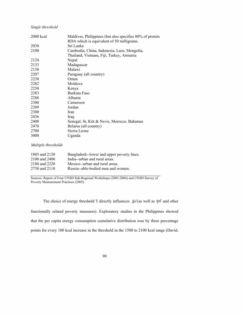
90
Single threshold 2000 kcal Maldives, Philippines (but also specifies 80% of protein
RDA which is equivalent of 50 milligrams. 2030 Sri Lanka 2100 Cambodia, China, Indonesia, Laos, Mongolia,
Thailand, Vietnam, Fiji, Turkey, Armenia 2124 Nepal 2133 Madagascar 2138 Malawi 2207 Paraguay (all country) 2238 Oman 2282 Moldova 2250 Kenya 2283 Burkina Faso 2288 Albania 2300 Cameroon 2309 Jordan 2300 Iran 2436 Iraq 2400 Senegal, St, Kitt & Nevis, Morocco, Bahamas 2470 Belarus (all country) 2700 Sierra Leone 3000 Uganda Multiple thresholds 1805 and 2120 Bangladesh--lower and upper poverty lines. 2100 and 2400 India--urban and rural areas. 2180 and 2220 Mexico--urban and rural areas. 2730 and 2110 Russia--able-bodied men and women. Sources: Report of Four UNSD Sub-Regional Workshops (2003-2004) and UNSD Survey of Poverty Measurement Practices (2005).
The choice of energy threshold T directly influences fpl (as well as tpl and other
functionally related poverty measures). Exploratory studies in the Philippines showed
that the per capita energy consumption cumulative distribution rose by three percentage
points for every 100 kcal increase in the threshold in the 1500 to 2100 kcal range (David,
91
2004).23 This implies that, given other factors remaining constant, changing the country�s
threshold from the official 2000 kcal to 2100 kcal used by majority of the developing
countries would result in a three-percentage point increase in the estimate of food poverty
incidence. Higher sensitivities are exhibited by results from Vietnam (Ministry of Health,
2003). The Bangladesh Bureau of Statistics previously used a variation called direct
calorie intake (DCI) method, alongside the CBN method. In the former, households and
members, whose calculated per capita energy consumption fell below a predetermined
threshold (2112 for urban and 2122 for rural), are considered food poor. The threshold
was lowered to 1805 kcal to estimate what the country calls the hard core or extremely
poor.
Results from 1983-84 to 1995-96 are summarized in Table 3. The 23.2 percent
average difference in poverty incidence between the 2120 kcal and 1805 kcal thresholds
imply a more than 7 percent shift per 100 kcal change in the assigned food poverty
threshold. Thus, the findings from the three countries raise the possibility that differences
in the countries� official energy thresholds (Table 2) could make incomparable national
poverty statistics as well as sub-national estimates (e.g., rural versus urban). If further
experiences from other countries support these findings, then the need for flexible or
robust alternative methodologies take on added importance (see Subsection 4.1.3 and
Section 4.2.
23 This occurs when per capita energy consumption is computed using family sizes adjusted for economies of scale as divisors of the estimated total family consumption. Using unadjusted family sizes led to higher sensitivity of the per capita energy consumption distribution in the same energy range.
92
Table 3. Bangladesh Food Poverty Incidences from DCI Method and Two Energy Thresholds (%)
.
Note: 2120 kcal is the average urban and rural thresholds, weighted by .20 and .80 population proportions, respectively. Source: From Counting the Poor to Making the Poor Count, World Bank, Bangladesh (1998).
4.1.2 Food basket construct and food poverty line ( fpl ) The next step to computing the food poverty line is to determine a bundle of food
� by item and weight, e.g., rice, 0.25kg and sugar, 0.03 kg � which provides a total (T�)
close to the specified threshold (say T, in kcal per person per day). The conversion is
made through a so-called food composition table from FAO/WHO that is adjusted by
individual countries to suit their individual situations. Basic data are obtained through a
Household surveys such as Household Food Consumption Survey (HFCS) or Household
Income and Expenditure Survey (HIES).
It is important that these surveys provide information for individual food items
consumed--by weight and value. Chapter 5 reviews in more details household surveys
used for poverty measurements. The composition of the food basket depends on the
choice of reference population. Since the object is to identify and count the poor, the
reference population is usually some lower percentile of households according to their
Year 2120 kcal 1805 kcal Difference 1983-84 62.6 36.8 25.8 1985-86 55.7 26.9 28.8 1988-89 47.8 28.4 19.4 1991-92 47.5 28.0 19.5 1995-96 47.5 25.1 22.4 Average - - 23.2
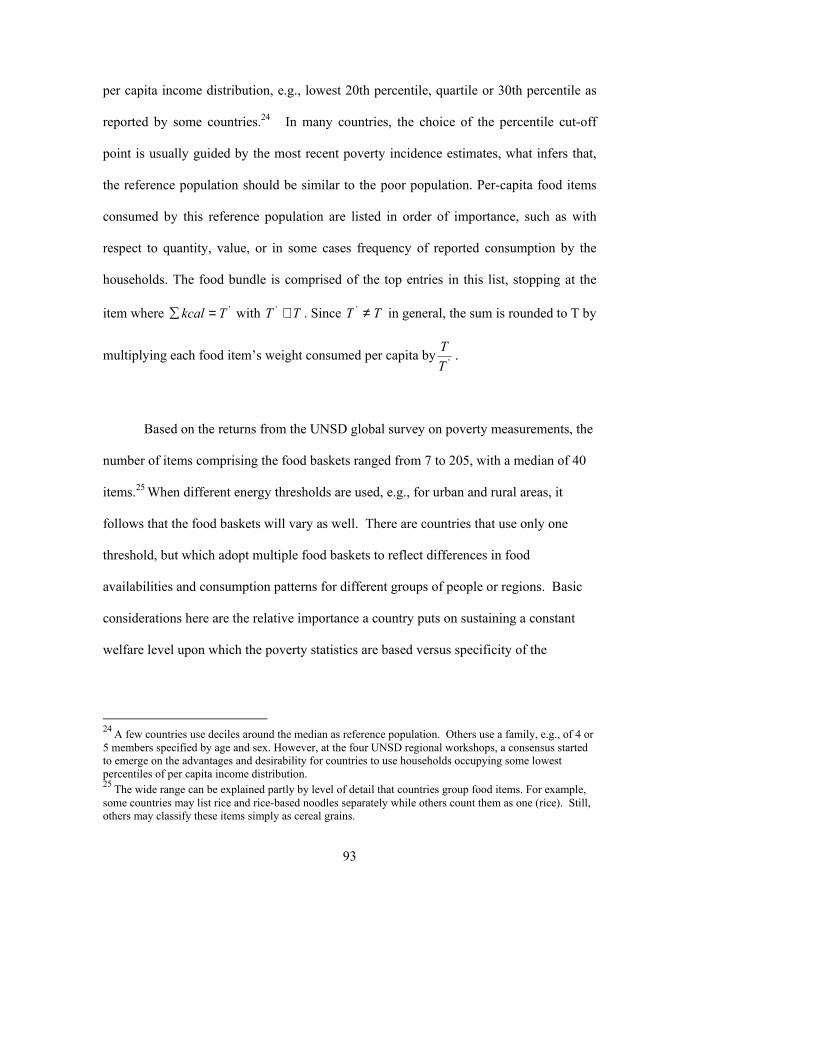
93
per capita income distribution, e.g., lowest 20th percentile, quartile or 30th percentile as
reported by some countries.24 In many countries, the choice of the percentile cut-off
point is usually guided by the most recent poverty incidence estimates, what infers that,
the reference population should be similar to the poor population. Per-capita food items
consumed by this reference population are listed in order of importance, such as with
respect to quantity, value, or in some cases frequency of reported consumption by the
households. The food bundle is comprised of the top entries in this list, stopping at the
item where 'Tkcal =∑ with TT ≅' . Since TT ≠' in general, the sum is rounded to T by
multiplying each food item�s weight consumed per capita by 'TT .
Based on the returns from the UNSD global survey on poverty measurements, the
number of items comprising the food baskets ranged from 7 to 205, with a median of 40
items.25 When different energy thresholds are used, e.g., for urban and rural areas, it
follows that the food baskets will vary as well. There are countries that use only one
threshold, but which adopt multiple food baskets to reflect differences in food
availabilities and consumption patterns for different groups of people or regions. Basic
considerations here are the relative importance a country puts on sustaining a constant
welfare level upon which the poverty statistics are based versus specificity of the
24 A few countries use deciles around the median as reference population. Others use a family, e.g., of 4 or 5 members specified by age and sex. However, at the four UNSD regional workshops, a consensus started to emerge on the advantages and desirability for countries to use households occupying some lowest percentiles of per capita income distribution. 25 The wide range can be explained partly by level of detail that countries group food items. For example, some countries may list rice and rice-based noodles separately while others count them as one (rice). Still, others may classify these items simply as cereal grains.
94
statistics to sub-national differences in food availability, preferences and consumption.
Let fqqq ,...,, 21 denote the quantities of the f items in the food basket that supply
feee ,...,, 21 respectively such that '21 ... Teee f =+++ kilocalories. Let fppp ,...,, 21 be the
unit prices of the f food items. The food poverty line is:
∑=f
ii pqTTfpl
1' (1)
Ideally, the prices should be period averages (usually one year) that the poor � or those in
the reference population � paid for the commodities in the food basket. In practice,
countries generally do not collect prices specifically for the purpose of compiling poverty
statistics. The prices used may come from varied sources, such as HIES or HFCS. Quite
often, however, what are collected in these surveys are quantity and expenditure for each
food commodity consumed or bought, such that the unit prices, though are not collected
directly, are derived by dividing the expenditure by the quantity of each commodity.
Participants in the UNSD sub-regional workshops reported that expenditure can
be accurately collected from households. However, quantity is relatively more
problematic, especially when the commodity is not traded in standard units. Thus, the
unit price derived from the two can at best be as reliable (or as inaccurate) as the quantity
estimate.26 Price quotes used for consumer price index (CPI) compilation are reused
routinely particularly, but not exclusively, for updating poverty lines. These have the
26 There was almost full unanimity in this opinion at the 2004 Sub-Regional Workshop of West African States wherein most of the participants were heads of national statistical offices.
95
advantage of providing average unit prices for the year for updating the poverty lines,
since majority of the developing countries maintain monthly or quarterly CPI series.
4.1.3 Alternative approaches to costing a food basket: Price per kcalorie and household level fpl Some countries avoid constructing a food basket by calculating the total
expenditure and total kcal content of all the food consumed by the reference population.
The ratio between the two totals is a price per kcal estimate. When this figure is
multiplied by the energy threshold, it provides an estimate of fpl . Once a price-per-kcal
estimate is calculated, fpl s for as many choices of energy thresholds are easily
computed. Indonesia used this approach until 1993 with different lists for urban and rural
areas (Maksum,C. 2004). Bangladesh, which as noted above uses two energy thresholds,
follows this approach in its direct calorie intake (DCI) method. The approach avoids unit
prices, which, as mentioned previously, are more difficult to obtain and may not even be
collected in some countries. However, the approach requires as many food expenditures
and conversion into energy equivalents as there are food commodities consumed by the
reference population.
Some countries do not report fpl separately (and related statistics, such as
incidence and number of food poor), since they see it merely as a necessary input in
calculating the total poverty line ( tpl ) and absolute poverty measures. This is unfortunate
because on their own food poverty statistics have important uses. They may also produce
more comparable statistics on the local and international levels than tpl and other more
96
composite poverty statistics. Two such more comparables statistics are discussed in this
chapter.
Another approach that has been implemented in a number of countries (Jordan,
Laos, and Thailand, as described for example, in Kakwani and Krongkaew, 1998,
involves taking the sum of the age x sex-specific RDAs of the members of the sample
household (∑RDA) (Kakwani, 2001). A household level food poverty line
[ kcM
PRDAhfpl ×= ∑ )( where ckP is the price per kcal and M the number of members in
the households] is computed and compared with the estimated total income or
expenditure (Y) of the household. All the members of the household are considered food-
poor if hfplY < , otherwise not. Note that unlike fpl which is determined on per capita
basis, hfpl and Y are household totals. From the survey, the design-weighted estimate of
the total of the Ms provides an estimate of the total number of food-poor in the sampled
population. This approach circumvents computing per capita energy consumption and per
capita income (expenditure) and the attendant problem of finding suitable adult
equivalents or scale economy-adjusted household sizes as divisors. (In Section 4.2, a
variation to Kakwani�s proposal is presented that eschews the use of prices and
currencies altogether.)
4.1.4 Computing the total poverty line ( tpl ) This computation involves two steps. The first defines essential non-food basic
needs and the second incorporates their cost into the food poverty line ( fpl ) to arrive at
97
the total poverty line ( tpl ). Simply put, fpl has to be adjusted upward by an amount
equal to or proportionate to the cost of procuring the essential non-food basic needs of a
poor or nearly poor person. Clearly, �essential non-food basic needs� requires a definition
that can be measured. Developing countries generally follow one of three operational
definitions or procedures.
A. List of specified essential non-food needs
This list is created usually by a group of users and stakeholders in association
with the national statistics office or the agency charged with producing the country�s
official poverty statistics. The list is exhaustive, covering items like clothing and
footwear, shelter, fuel and light, household goods, health services, personal care, and
education. Costs per person are assigned to each item. Hence, if nfpl (non-food poverty
line) denotes the sum of the costs, then:
nfplfpltpl += (2)
This was the procedure of choice by some countries during their early years of poverty
statistics compilation, and some still keep it as part of their official methodology (e.g.,
Indonesia, see Maksum, op. cit.).
Simplicity is its main appeal. However, the outcome is very much dependent on a
highly subjective list. Adding or subtracting from the list affects tpl directly in an
additive fashion. It is easy for anyone to criticize why this item is included while that
item is not. Changes in the list would affect the comparability of the tpl time series.
Similarly, different lists for different areas or sub-populations result in non-comparable
98
statistics, for example, bread plus rice in cities versus all rice in rural areas or physician-
attended childbirth in urban regions versus midwife-assisted deliveries in rural areas.
B. Regression
This approach comes from the World Bank (see Ravallion, 1992) and is premised
on a particular definition of essential non-food basic needs. A household whose total
expenditure per capita ( te ) is equal to fpl still has to spend for items other than food, and
those items must be regarded as essential by the household. The set of non-food items
availed of by households for whom fplte = may then be considered to define essential
non-food needs. And the average expenditure of the households for the set may be used
to estimate nfpl in equation (3.2). The problem is that none or few households will
precisely satisfy fplte = . One solution is to run a simple linear regression of the share of
per capita food expenditure ( fe ) to total expenditure, (tefeS = ), on )log(
fplte using data
from the reference poor population. That is: iii errorfplteS ++= )log(βα
where i runs through the sample households in the reference population. Let α� be the
estimate of the interceptα . Since 0)log( =fplte when fplte = , it follows that α� provides
an estimate of the food share among households whose total expenditures match the food
poverty line. Conversely, α�1− estimates the essential non-food share. Hence,
fplfpltpl )�1( α−+= , or fpltpl )�2( α−= (3)
99
For example, China used this method in its 1995 Rural Household Survey and
obtained food share 83.0� =α , hence fpltpl 17.1= = Renminbi 557. Before 1995, China
used fpltpl 40.1= , where the 40 percent adjustment was based on what was then the
experts� opinion of a �reasonable food share� of 60 percent. The big reduction in the
adjustment factor from 40 percent to 17 percent naturally led to speculations that the pre-
1995 estimates are not comparable to those from 1995 onward. However, from 2003,
China started recompiling a second set of poverty statistics based on the pre-1995 60
percent food share. Other countries, in particular those who received World Bank
assistance to conduct living standard surveys and poverty analysis, such as Cambodia,
Mongolia, and Vietnam in the Asian region, have followed the regression approach.
As a food share, α is an Engel�s coefficient, albeit in a very restricted sense, i.e.,
when tefpl = . As such, the quantity α�fpl is an estimate of the total poverty line as well.
However, an Engel coefficient computed directly from the households returns may be the
more appropriate divisor for this form of tpl estimate. Also, the inequality fplte > is
expected to hold for most sample households in the reference population. Otherwise,
0)log( <fplte . If this happens in a sizable subset of the sample, the regression equation
may not provide a good fit to the data. A more attractive alternative in this case is direct
estimation of Engel�s coefficient.
100
C. Engel�s coefficient
Many countries use a more pragmatic approach to determine the total poverty
line. They compute Engel�s coefficient tefe directly from the sample households with
expenditures within a given (say ±d) percentage points of fpl . 10=d percent is a
common choice among the countries (e.g in Lao PDR and Philippines). Similarly, as in
the regression method, tpl may be computed as
fpltefetpl )2( −= (4)
Why 10 percent and not 5 percent or some other per capita expenditure band around
fpl ? Countries often base their choice on neighboring country practice or on a
consultant�s recommendation. It is preferable to base the choice on empirical evidence by
calculating tefe for several values of d. Figure 1 shows an example where
tefe was
computed from the Philippines 1994 Family Income and Expenditure Survey data with d
ranging from 2 to 20 percent. The Engel coefficient seems to be robust for d in the 2 to 5
percent range. But it begins to decline continuously as d approaches 10 percent. The
coefficient behaves differently for rural and urban areas, with the latter exhibiting
markedly lower value, hence higher tpl . This is to be expected as urban dwellers
generally pay more than rural residents for housing, transport and other essential non-
food goods and services. This raises an issue whether one national tpl is all that is
needed or whether separate tpl s should be computed for the urban and rural areas.
Figure 1. Ratio of Food Expenditures to Total Expenditures, 1994, Philippines Formatted: Font: Bold
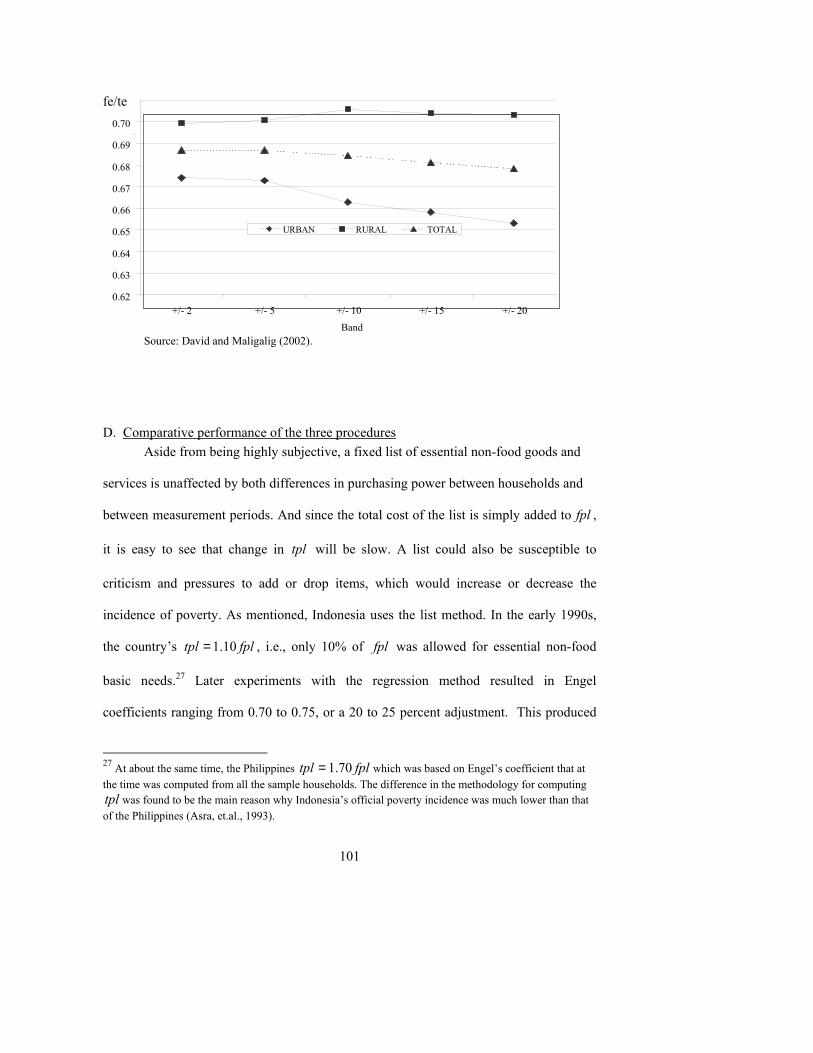
101
Source: David and Maligalig (2002).
D. Comparative performance of the three procedures Aside from being highly subjective, a fixed list of essential non-food goods and
services is unaffected by both differences in purchasing power between households and
between measurement periods. And since the total cost of the list is simply added to fpl ,
it is easy to see that change in tpl will be slow. A list could also be susceptible to
criticism and pressures to add or drop items, which would increase or decrease the
incidence of poverty. As mentioned, Indonesia uses the list method. In the early 1990s,
the country�s fpltpl 10.1= , i.e., only 10% of fpl was allowed for essential non-food
basic needs.27 Later experiments with the regression method resulted in Engel
coefficients ranging from 0.70 to 0.75, or a 20 to 25 percent adjustment. This produced
27 At about the same time, the Philippines fpltpl 70.1= which was based on Engel�s coefficient that at the time was computed from all the sample households. The difference in the methodology for computing tpl was found to be the main reason why Indonesia�s official poverty incidence was much lower than that of the Philippines (Asra, et.al., 1993).
0.62 0.63 0.64 0.65 0.66 0.67 0.68 0.69 0.70
+/- 2 +/- 5 +/- 10 +/- 15 +/- 20Band
fe/te
URBAN RURAL TOTAL
102
significantly higher poverty incidence levels. These coefficients, however, have not been
adopted, and the current official methodology remains based on separate lists of essential
non-food goods and services for the rural and urban areas (Said and Widyanti, 2001).
Regression and direct use of Engel�s coefficient can be expected to lead to similar
tpls , particularly when the latter is computed from a sub-sample of households falling
inside a narrow band, say those with per capita expenditures within ± (2 to 5) per cent of
fpl . The sub-sample, however, gets smaller as the band is narrowed. Since a bigger sub-
sample implies a more precisetefe estimate, there are instances where a band as wide as 10
percent is justified. Compared to running regressions, estimating tefe directly may be less
taxing to the national statistics office, especially if this has to be done for every HIES.
This also avoids problems resulting from a poor linear regression fit.
Instead of scaling up fpl to tpl in a linear fashion, as in equation (2), some
countries opt to use the non-linear estimate:
α�fpltpl = or
tefefpltpl = (5)
In other words, the total poverty line is the ratio of the food poverty line to Engel�s
coefficient. The Philippines� official poverty statistics, for example, are computed based
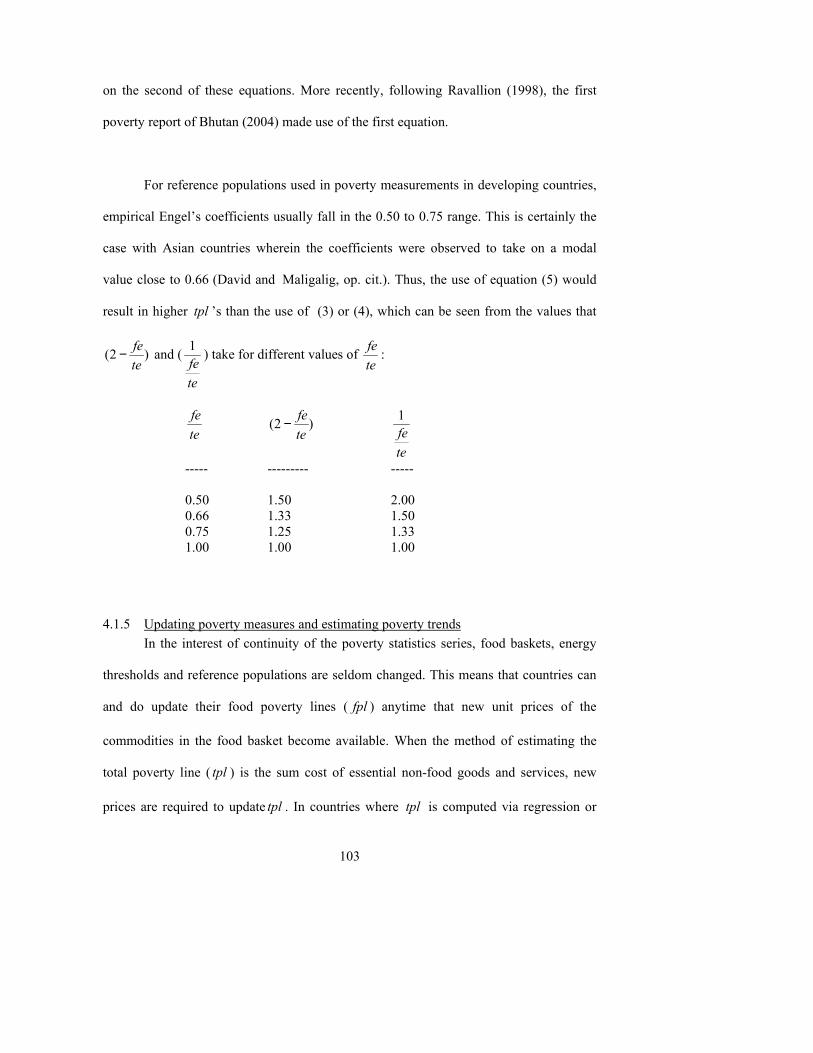
103
on the second of these equations. More recently, following Ravallion (1998), the first
poverty report of Bhutan (2004) made use of the first equation.
For reference populations used in poverty measurements in developing countries,
empirical Engel�s coefficients usually fall in the 0.50 to 0.75 range. This is certainly the
case with Asian countries wherein the coefficients were observed to take on a modal
value close to 0.66 (David and Maligalig, op. cit.). Thus, the use of equation (5) would
result in higher tpl �s than the use of (3) or (4), which can be seen from the values that
)2(tefe− and (
tefe1 ) take for different values of
tefe :
tefe )2(
tefe−
tefe1
----- --------- ----- 0.50 1.50 2.00 0.66 1.33 1.50 0.75 1.25 1.33 1.00 1.00 1.00
4.1.5 Updating poverty measures and estimating poverty trends In the interest of continuity of the poverty statistics series, food baskets, energy
thresholds and reference populations are seldom changed. This means that countries can
and do update their food poverty lines ( fpl ) anytime that new unit prices of the
commodities in the food basket become available. When the method of estimating the
total poverty line ( tpl ) is the sum cost of essential non-food goods and services, new
prices are required to update tpl . In countries where tpl is computed via regression or
104
Engel�s coefficient, updating is sometimes done by using the same coefficient for the
years that a HIES is not done. It is assumed implicitly that the coefficient either does not
change or changes very slowly in the reference population during a one-to-two year
period. Coefficients are recomputed only when there is a new HIES round.
Sometimes the CPI is used (e.g., the food CPI and non-food CPI) to update the
food and non-food components of the total poverty line. It has been noted, however, that
the CPI as currently constructed in most countries might not reflect the consumption
pattern of the reference population used in determining the poverty lines (see discussion
in Subsection 4.1.2). Another key limitation is that the basket of goods used for the CPI
may vary significantly from the one used to construct the poverty lines. These limitations
can be more pronounced when estimating sub-national poverty lines. Some countries
address these issues by using sub-national CPIs constructed from household survey data
(e.g., Sri Lanka, Vietnam and Thailand). Sticking to the same mode of updating is
important for the country�s poverty lines to be comparable across time. Updating the
statistics on the number and proportion of poor persons or households will require new
estimates of per capita income (expenditure) distributions which in turn require a new
HIES round. Very few users would be willing to assume that these distributions remain
constant even over a single year because doing so would nullify the need to update the
poverty statistics in the first place. These updates are discussed in greater detailed in
Chapters 5 and 7. As obvious as this seems, its practical implications seem to be lost to
some users at times. It is not unheard of that users want annual updates on the estimates
of the number and proportion of poor persons (households), which means that a HIES is
105
conducted yearly at great cost. And sample sizes, hence human and material
requirements, rise even more as users demand that the updates be done for progressively
smaller sub-populations.28
Some of the countries that update poverty counts and incidences annually (e.g.,
China) simplify the methodology by having one national poverty line and releasing
national level estimates only. This keeps the survey sample size relatively small. Doing
otherwise, such as updating annually at sub-national levels, could quickly lead to very
large surveys. For example, Indonesia�s annual socio-economic survey has a sample size
of 200,000 households (see Surbakti, et. al, 2001). This would delay release of results,
defeating the purpose of updating yearly. If user demands are not aligned with the
technical and material resources available to the national statistical system, the poverty
monitoring system soon becomes unsustainable.
The frequency in which poverty incidences and counts are updated for various
countries-- which coincides with the frequency of conducting household income and
expenditure surveys--is shown in Table 4. The frequency ranges from one to five years
for nations with a poverty monitoring program. This is not to say that countries that
follow the same updating frequency of, say every three years, track the same reference
years. Many countries still have no regular schedule of updating, inasmuch as a HIES is
conducted only when funds become available, usually from an external donor. Of the 107
countries that responded to the UNSD 2005 Survey of Poverty Measurement Practices,
28 What matters is little n, not n/N , where n is the sample size in the smallest domain of interest -- is a truism that needs repeating every so often.
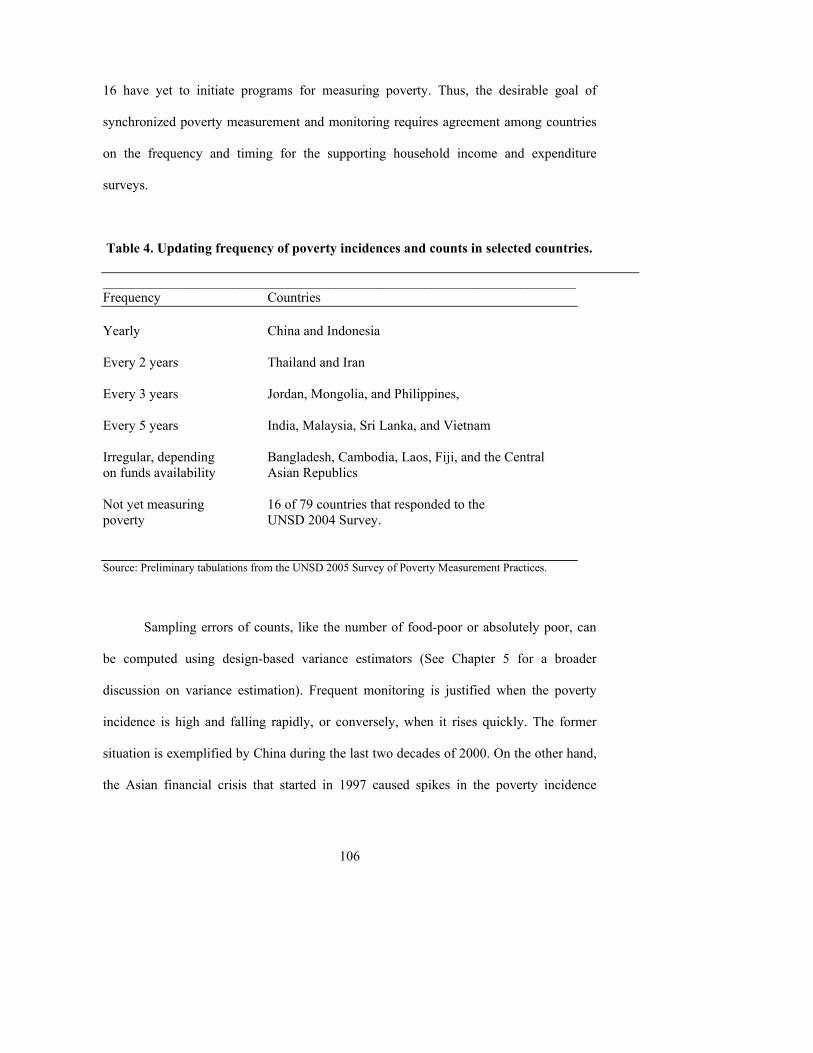
106
16 have yet to initiate programs for measuring poverty. Thus, the desirable goal of
synchronized poverty measurement and monitoring requires agreement among countries
on the frequency and timing for the supporting household income and expenditure
surveys.
Table 4. Updating frequency of poverty incidences and counts in selected countries.
_____________________________________________________________________ Frequency Countries Yearly China and Indonesia Every 2 years Thailand and Iran Every 3 years Jordan, Mongolia, and Philippines, Every 5 years India, Malaysia, Sri Lanka, and Vietnam Irregular, depending Bangladesh, Cambodia, Laos, Fiji, and the Central on funds availability Asian Republics Not yet measuring 16 of 79 countries that responded to the poverty UNSD 2004 Survey.
Source: Preliminary tabulations from the UNSD 2005 Survey of Poverty Measurement Practices.
Sampling errors of counts, like the number of food-poor or absolutely poor, can
be computed using design-based variance estimators (See Chapter 5 for a broader
discussion on variance estimation). Frequent monitoring is justified when the poverty
incidence is high and falling rapidly, or conversely, when it rises quickly. The former
situation is exemplified by China during the last two decades of 2000. On the other hand,
the Asian financial crisis that started in 1997 caused spikes in the poverty incidence
107
among severely affected countries such as Thailand and Indonesia. This had been
described as transitory poverty brought about by stagflation--economic contraction and
precipitous currency devaluation. Poverty monitoring frequency was briefly increased to
twice a year and then reverted to a yearly frequency in these countries. Now that the
poverty incidence in Thailand has returned to pre-crisis levels of about 10 percent,
monitoring has been scaled back to once every two years. As mentioned previously,
China and Indonesia continue to update their poverty incidence levels annually. With
China�s official (rural) poverty incidence estimated under 6 percent, the amount of
reduction that can be achieved in a year�s time is naturally very much constrained. Hence,
the chance of detecting a change through statistical means will require a very efficient
and large household income survey. (Although China uses both income and expenditure,
the former is the basis for the officially released poverty statistics.)
4.1.6 Relative and subjective income/expenditures based poverty lines Income-based relative poverty lines often are simple functions of the median or
mean of the per capita income distribution. These relative poverty lines are much easier
to establish and are suitable for quickly finding out who are poor and where they live.
When applied to small areas, they could be used to classify individuals as well as rank
communities, thereby enabling sharper allocation of poverty reduction resources in a
relatively short time. However, estimates are influenced by shifts in the central values as
well as shape of the per capita income distribution. Therefore, they are not meant to be
used to monitor the poverty situation from one period to another.
108
Relative poverty lines are more frequently used by developed than developing
countries and it practice varies also among the countries. A number of countries in The
Economic Commission for Latin America & the Caribbean (ECLAC) region for example
have used 50 percent of the median per capita income (Rio Group Report, 2003). Oman
instead defines as poor a person with income less than 40 percent of the population�s
median per capita income (UNSD-ESCWA Sub-Regional Poverty Statistics Workshop
Report, November 2004) while Iran uses 50 percent of both the mean and median per
capita incomes (UNSD-ESCAP Sub-Regional Poverty Statistics Workshop Report,
October 2004)
Country experience in subjective poverty lines is very limited and still not well
established. In the Philippines, a private market research organization asks heads of
households about their income: whether they consider themselves poor, and if so, how
much more income would they need not to consider themselves as poor. This �self-
assessed poverty� approach yields what are sometimes referred to as subjective poverty
estimates. Like many opinion poll-type investigations, these surveys are small. They
typically involve 1200 - 1500 sample households, enabling the results to be released very
quickly. Egypt�s national statistical system has constructed a subjective poverty line
based also on minimum income that household heads believe is necessary for an adequate
standard of living. The experience of Egypt showed, however, that this methodology
overestimates poverty, especially in urban areas where expectations of educated
household heads tend to exceed current income levels by a large margin (UNSD-
ESCWA, op. cit).
109
4.2 Direct measures of food poverty
4.2.1 Estimating the empirical cumulative distribution function (cdf) of per capita energy consumption
As implemented by countries, the cost of basic needs (CBN) approach discussed
in Section 4.1 yields one set of food poverty statistics for each specification of the energy
threshold T. This means non-comparable statistics for countries and sub-national domains
that adopt different Ts (see Table 2). One way out of this predicament is to estimate the
entire per capita energy consumption cdf, that is, divide the calculated total energy
consumption (∑kcal) of the household by some measure of the number of consuming
members. This is done in some countries, but generally not in the agencies charged with
producing official statistics. For example, Vietnam�s General Statistics Office (GSO)
uses the CBN method in compiling the official poverty statistics from its Multipurpose
Household Survey and Vietnamese Living Standards Survey. The official population
food poverty incidence estimates for 1998 and 2002 were 15.0% and 10.9%, respectively
(Vietnam Development Report 2004). The National Institute of Nutrition of the Ministry
of Health conducts a General Nutrition Survey (GNS) in which household food
consumption is obtained via a different data-capture method described as a 24-hour recall
combined with weighing of some of the food items .
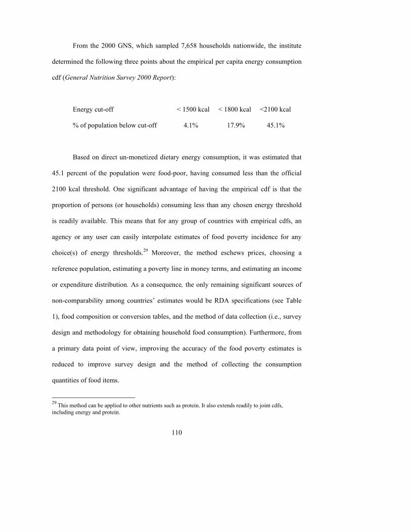
110
From the 2000 GNS, which sampled 7,658 households nationwide, the institute
determined the following three points about the empirical per capita energy consumption
cdf (General Nutrition Survey 2000 Report):
Energy cut-off < 1500 kcal < 1800 kcal <2100 kcal
% of population below cut-off 4.1% 17.9% 45.1%
Based on direct un-monetized dietary energy consumption, it was estimated that
45.1 percent of the population were food-poor, having consumed less than the official
2100 kcal threshold. One significant advantage of having the empirical cdf is that the
proportion of persons (or households) consuming less than any chosen energy threshold
is readily available. This means that for any group of countries with empirical cdfs, an
agency or any user can easily interpolate estimates of food poverty incidence for any
choice(s) of energy thresholds.29 Moreover, the method eschews prices, choosing a
reference population, estimating a poverty line in money terms, and estimating an income
or expenditure distribution. As a consequence, the only remaining significant sources of
non-comparability among countries� estimates would be RDA specifications (see Table
1), food composition or conversion tables, and the method of data collection (i.e., survey
design and methodology for obtaining household food consumption). Furthermore, from
a primary data point of view, improving the accuracy of the food poverty estimates is
reduced to improve survey design and the method of collecting the consumption
quantities of food items.
29 This method can be applied to other nutrients such as protein. It also extends readily to joint cdfs, including energy and protein.
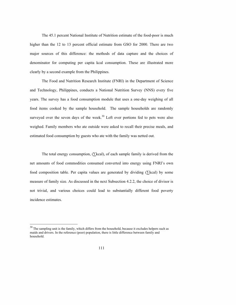
111
The 45.1 percent National Institute of Nutrition estimate of the food-poor is much
higher than the 12 to 13 percent official estimate from GSO for 2000. There are two
major sources of this difference: the methods of data capture and the choices of
denominator for computing per capita kcal consumption. These are illustrated more
clearly by a second example from the Philippines.
The Food and Nutrition Research Institute (FNRI) in the Department of Science
and Technology, Philippines, conducts a National Nutrition Survey (NNS) every five
years. The survey has a food consumption module that uses a one-day weighing of all
food items cooked by the sample household. The sample households are randomly
surveyed over the seven days of the week.30 Left over portions fed to pets were also
weighed. Family members who ate outside were asked to recall their precise meals, and
estimated food consumption by guests who ate with the family was netted out.
The total energy consumption, (∑kcal), of each sample family is derived from the
net amounts of food commodities consumed converted into energy using FNRI�s own
food composition table. Per capita values are generated by dividing (∑kcal) by some
measure of family size. As discussed in the next Subsection 4.2.2, the choice of divisor is
not trivial, and various choices could lead to substantially different food poverty
incidence estimates.
30 The sampling unit is the family, which differs from the household, because it excludes helpers such as maids and drivers. In the reference (poor) population, there is little difference between family and household.
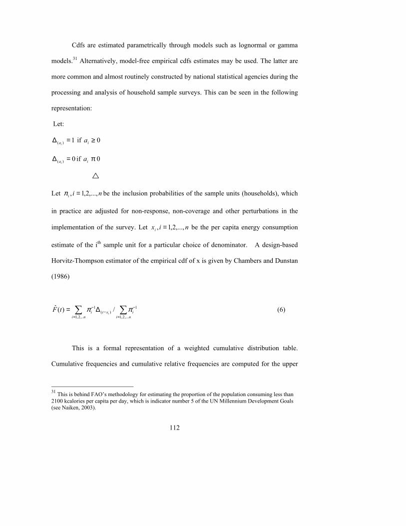
112
Cdfs are estimated parametrically through models such as lognormal or gamma
models.31 Alternatively, model-free empirical cdfs estimates may be used. The latter are
more common and almost routinely constructed by national statistical agencies during the
processing and analysis of household sample surveys. This can be seen in the following
representation:
Let:
1)( =∆ia if 0≥ia
0)( =∆ia if 0πia
Let nii ,...,2,1, =π be the inclusion probabilities of the sample units (households), which
in practice are adjusted for non-response, non-coverage and other perturbations in the
implementation of the survey. Let nixi ,...,2,1, = be the per capita energy consumption
estimate of the ith sample unit for a particular choice of denominator. A design-based
Horvitz-Thompson estimator of the empirical cdf of x is given by Chambers and Dunstan
(1986)
∑ ∑= =
−−
− ∆=ni ni
ixti itF
,..2,1 ,...2,1
1)(
1 /)(� ππ (6)
This is a formal representation of a weighted cumulative distribution table.
Cumulative frequencies and cumulative relative frequencies are computed for the upper
31 This is behind FAO�s methodology for estimating the proportion of the population consuming less than 2100 kcalories per capita per day, which is indicator number 5 of the UN Millennium Development Goals (see Naiken, 2003).
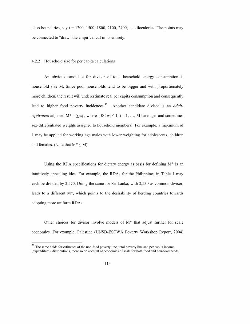
113
class boundaries, say t = 1200, 1500, 1800, 2100, 2400, � kilocalories. The points may
be connected to �draw� the empirical cdf in its entirety.
4.2.2 Household size for per capita calculations
An obvious candidate for divisor of total household energy consumption is
household size M. Since poor households tend to be bigger and with proportionately
more children, the result will underestimate real per capita consumption and consequently
lead to higher food poverty incidences.32 Another candidate divisor is an adult-
equivalent adjusted M* = ∑wi , where { 0< wi ≤ 1; i = 1, �, M} are age- and sometimes
sex-differentiated weights assigned to household members. For example, a maximum of
1 may be applied for working age males with lower weighting for adolescents, children
and females. (Note that M* ≤ M).
Using the RDA specifications for dietary energy as basis for defining M* is an
intuitively appealing idea. For example, the RDAs for the Philippines in Table 1 may
each be divided by 2,570. Doing the same for Sri Lanka, with 2,530 as common divisor,
leads to a different M*, which points to the desirability of herding countries towards
adopting more uniform RDAs.
Other choices for divisor involve models of M* that adjust further for scale
economies. For example, Palestine (UNSD-ESCWA Poverty Workshop Report, 2004)
32 The same holds for estimates of the non-food poverty line, total poverty line and per capita income (expenditure), distributions, more so on account of economies of scale for both food and non-food needs.
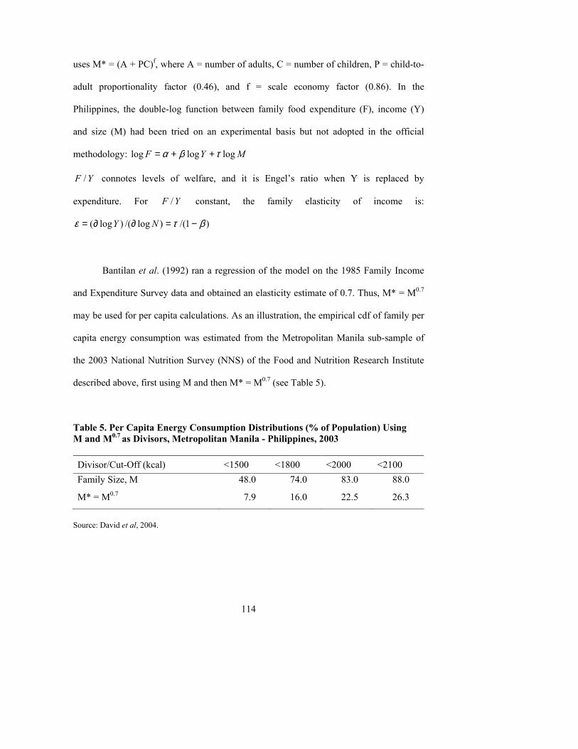
114
uses M* = (A + PC)f, where A = number of adults, C = number of children, P = child-to-
adult proportionality factor (0.46), and f = scale economy factor (0.86). In the
Philippines, the double-log function between family food expenditure (F), income (Y)
and size (M) had been tried on an experimental basis but not adopted in the official
methodology: MYF logloglog τβα ++=
YF / connotes levels of welfare, and it is Engel�s ratio when Y is replaced by
expenditure. For YF / constant, the family elasticity of income is:
)1/()log/()log( βτε −=∂∂= NY
Bantilan et al. (1992) ran a regression of the model on the 1985 Family Income
and Expenditure Survey data and obtained an elasticity estimate of 0.7. Thus, M* = M0.7
may be used for per capita calculations. As an illustration, the empirical cdf of family per
capita energy consumption was estimated from the Metropolitan Manila sub-sample of
the 2003 National Nutrition Survey (NNS) of the Food and Nutrition Research Institute
described above, first using M and then M* = M0.7 (see Table 5).
Table 5. Per Capita Energy Consumption Distributions (% of Population) Using M and M0.7 as Divisors, Metropolitan Manila - Philippines, 2003 Divisor/Cut-Off (kcal) <1500 <1800 <2000 <2100 Family Size, M 48.0 74.0 83.0 88.0
M* = M0.7 7.9 16.0 22.5 26.3
Source: David et al, 2004.
115
Predictably, the results with M lead to very high food poverty incidence rates. At
the official 2000 kcal threshold, it is an unrealistically high 83 percent. Other researchers
observed this phenomenon, and it appeared in the Vietnam case mentioned above. The
empirical cdf, with scale-economy-adjusted family size as divisor, leads to much lower
food poverty incidence rates. One advantage of a cdf estimate is seeing the effect that a
change in energy threshold will have on the incidence. For example, moving the
Philippines� official 2000 kcal threshold to 2100 kcal, which is used by the majority of
Asian countries, would mean about a four percentage point increase in the estimated food
poverty incidence for metropolitan Manila, from 22.5 percent to 26.3 percent.
From the UNSD�s regional workshops and 2005 poverty practices survey, it
appears that many of the developing countries use household size (M) to compute per
capita food and non-food consumption, as well as per income and expenditure. Others
use some adjustment only a step or two removed from M. For example, Senegal uses
only two weights: w1 = 0.5 for household members below 15 years old, and w2 = 1.0 for
all others. Some use adult equivalents based directly on the RDA specifications. But this
is usually for calculating per capita food consumption only. Very few use any adjustment
in estimating per capita income or expenditure. The likely effect could be overestimated
poverty incidences and counts.33 Alternatively, in so far as food poverty is concerned, per
capita food consumption, thresholds, income and expenditure may be circumvented
altogether.
33 Countries that attended the UNSD sub-regional poverty workshops expressed significant interests in technical information and assistance in implementing adult equivalent and/or economies of scale adjusted per capita methods.
116
4.2.3 Eschewing per capita calculations
Most countries have developed their respective per capita RDAs for dietary
energy, as well as for other nutrients, for different age-by-sex groupings of their
populations (see Table 1). Those that have not, have either adopted their neighboring
countries� standards or the latest recommendations of FAO or WHO. Instead of resorting
to a per capita threshold for the household, it is natural to regard the sum of the RDAs of
a household, ∑RDA, as the energy threshold for that particular household. Thus, if ∑kcal
represents the estimated daily total energy consumption of the same household, the
inequality ∑kcal < ∑RDA can be used directly to classify households and persons therein
as either food poor or non-food poor.
More than one set of RDAs may be considered, giving rise to as many thresholds
and food poverty estimates. For example, a 1971 FAO/WHO Expert Committee on
Energy and Protein Requirements accepted a 15 percent coefficient of variation of energy
requirement between individuals in a population or group with similar demographics
(WHO, 1985, p. 6). Hence, reducing the individual RDAs proportionately by 15 percent
and by 30 percent will yield ∑RDAs that correspond approximately with minus one and
minus two standard deviations from the original respectively. Similarly, increasing the
individual RDAs by the same amounts will correspond with plus one and plus two
standard deviations from the original ∑RDA. Six-point estimates together provide a fuller
understanding of the relationship between RDA specifications and thresholds, along with
poverty measures. Comparable food poverty estimates across and within a country can be
interpolated easily for any given choice of household threshold within the
117
(1 ± 0.3) ∑RDA interval.
The weighted sum of the energy shortfall among the food poor households is a
direct estimate of an energy gap:
Energy gap = ∑w{∑RDA - ∑kcal} if {∑RDA - ∑kcal} > 0 (7)
= 0 otherwise
where the inner summations run through the members of the household, w denotes the
design weight of the sample household, and the outer summation runs through all sample
households. The energy gap estimates the amount of dietary kilocalories needed to bring
all the food poor families up to their respective food poverty thresholds. If desired, this
can be expressed in monetary terms by multiplying by the cost per kcal (obtained from
the reference population). This simple and straightforward interpretation of this statistic
can have mass appeal to policy makers and lay persons alike.
4.3 Non-income measurement methods
The minimum basic needs (MBN) (also called unmet basic needs (UBN))
approach has been used in a number of countries in lieu or in addition to the income-
based basic needs approach. In this approach non-monetary indicators representing
different dimensions of poverty are chosen, estimated and monitored. The subset of
118
Millennium Development Goals [MDGs] minus the income indicators provides excellent
examples:
• Proportion of underweight children to represent malnutrition;
• School enrollment, primary school completion, and youth illiteracy rates to
represent basic education;
• Infant and under-five mortality rates, maternal mortality ratio, and births attended
by skilled health staff to represent primary health care; and the
• Ratio of girls to boys in primary and secondary school, ratio of literate females to
males, proportion of seats held by women in parliament, and share of women
employed in the non-agriculture sector to represent the gender equality dimension
or goal.
Many, though not all, of these indicators are long-term outcomes or output
indicators. Case in point: a child being underweight is the result of years of chronic
undernourishment. Also, these UBN indicators are expressed in different units of
measure. This has made producing a composite index a difficult and perpetually
subjective task. However, this has not prevented agencies, particularly international
bodies, from constructing such indexes. These include the Human Development Index
(HDI) and other indices that UNDP puts out annually for each country in Human
Development Report. These may have added value more as devices for advocacy than as
monitoring tools. Few developing countries compile composite indexes, preferring to use
the indicators individually and collectively in much the same way that they will be used
to monitor progress in the MDGs.
119
National statistical systems have also been compiling many of the UBN indicators
long before the international development agencies declared poverty reduction their
overriding strategic objective. Many are extracted from population and housing
censuses, demographic and health surveys, civil registries and other administrative
reporting systems. In fact, choice of indicators in a country�s UBN information system is
often determined by existing data collection systems; seldom is a new system established
just to meet the additional requirements for new indicators. This is the case in
Bangladesh, for example, where infant mortality is used as a proxy indicator for the
primary health care system, primary school enrollment rate for basic education, and
housing characteristics (access to tap water, toilet facilities, and electricity, and building
materials used) for living conditions.
Nearly all countries in ECLAC have UBN poverty monitoring systems in place
(Rio Group Report, May 2004). However, unlike income poverty statistics compilations,
there are differences in the selection of dimensions and indicators for the basic needs,
partly owing to variations in data availability. The three broad categories of basic needs
often considered are dwelling characteristics, access to safe water, and access to
sanitation facilities. Basic education and economic capacity (e.g., GDP growth rate) are
sometimes included in an expanded UBN set of indicators. In the ECLAC, the UBN
approach has a solid conceptual foundation as it measures actual satisfaction or
dissatisfaction of needs rather than the capacity to satisfy them. In this light, it is
complementary to the income poverty line approach. Dimensions of basic needs chosen
120
are often those highly correlated with income, so much so that they have been used to
identify households under extreme poverty.
Assessment and monitoring of poverty through the UBN approach is far from
widespread in Africa. Only three of the 10 members of the Economic Community of
Western African States (ECOWAS) acknowledge having a UBN system in place. The
main poverty dimensions considered are basic education, primary health, and housing
characteristics, such as access to safe water, toilet facilities and building materials used.
UBN methods can and are being brought down to sub-national levels. For example,
China monitors community level indicators, such as percent of villages accessible by
roads, percent with land-line phone connections, percent with electricity, illiteracy rates,
child enrollment rates, and labor migration rates.
4.4 Conclusion
National statistical information systems have evolved to a point that developing
countries more or less follow similar updating frequencies for certain parts of their
socioeconomic databases. Thus, censuses have a ten-year cycle, demographic and health
surveys five years, nutrition surveys three to five years, and agricultural surveys one
season or one year. Being relatively new, poverty statistics have not had enough time to
be part of this evolution. The IMF has formalized the frequencies of statistical series in its
General Data Dissemination System (GDDS) and Special Data Dissemination System
121
(SDDS). For example, countries that subscribe to GDDS agree to update their price
indexes monthly, and those that sign up on SDDS agree to compile national accounts
quarterly. However, poverty statistics are not covered adequately in these dissemination
systems.
As seen in Table 4, the frequency of updating of poverty incidence and related
statistics varies significantly at the national level. Individual countries have their own
reasons for choosing a particular updating frequency. The choice is often a compromise
between the users� desire for more frequent updating at smaller domains versus the
limited resources available to fund surveys repeatedly. Ultimately, financing and the
desired accuracy and timeliness of the results are the key factors determining survey
frequency.
As mentioned previously, poverty lines can be updated more frequently using new
price data. However, updating poverty incidences and counts require current estimates of
per capita income or expenditure distributions, i.e., a new HIES round. The high cost of
an HIES makes the majority of developing countries decide on a three-to-five-year
poverty monitoring program. If more frequent updating is desired, one strategy that has
some chance of being sustained is where this is done for national level estimates only and
based on a smaller sample; sub-national estimates may be updated less frequently for
which a relatively larger sample is required.
122
Variations in updating frequency increase when poverty information compilation
and monitoring at sub-national levels done by stakeholders, other than the national
statistical office, are included. Demand for sub-national poverty statistics come from
local officials, central government agencies, non-government organizations (including
resident missions of international bodies that focus their interventions on specific
disadvantaged groups or areas), and analysts.
Central governments, analysts, and international agencies require country-level
poverty statistics. Some need annual updates to feed into their global monitoring
activities, including the UNDP�s Human Development Report, World Bank�s World
Development Report, FAO�s State of Food Insecurity, and the UN Secretary General�s
annual progress on the MDGs report to the General Assembly. These agencies put up
internal capacities for estimating, interpolating, or projecting from past and current (but
partial) information from countries. These agencies are the main sources of poverty
information at the regional or global levels. They do not run into problems of
inconsistency or non-comparability since countries are not involved in similar activities.
It is when the international agencies also publish their own produced national estimates
that non-comparability with the countries� statistics can and do arise.
In general, national statistics offices (NSOs) are able to provide some of the
needed data at the level of villages, districts, ethnicity and other socio-demographic
groupings during census years only. Traditional inter-census national sample surveys can
provide reasonably precise statistics for only large domains, such as urban and rural
123
regions. NSOs will have to continue these surveys to monitor poverty at these macro-
levels, as well as to provide input data for monitoring at the global level.
They could not hope to have the time to muster resources required to successfully
launch sample surveys with adequate sample sizes for areas below regions and domains
of special interest, such as ethnic groups, the handicapped, and similar vulnerable
segments of the population. However, information is needed for these smaller domains
for more efficient targeting of poverty alleviation, as well as for monitoring and
evaluating the impact of such interventions.
Strategies for filling these data gaps in small domains are critically needed.
Specialized agencies and ministries responsible for planning and implementing sub-
national poverty reduction programs will help generate needed information at these
levels.
For example, Thailand�s Ministry of Interior conducts an annual Basic Minimum
Needs Survey to identify villages eligible for poverty alleviation assistance. There were
attempts in Cambodia and Laos to construct district vulnerability indexes from village-
level participatory poverty assessment censuses or surveys. A complete enumeration of
households is carried out by Vietnam�s Ministry of Labor, Invalids and Social Affairs
(MOLISA) to identify poor households that qualify to receive subsidies. Indonesia�s
Central Bureau of Statistics and National Planning Board collaborate to annually measure
the welfare level of each household, to identify those eligible to receive poverty
124
subsidies, and to determine the amount of assistance (Surbakti et al, 2001). Moreover,
administrative records of the above ministries as well as those of education, health, and
civil registrations are important sources of poverty information for small domains.
It is important not to expect results from these different sources and methods to be
consistent or comparable. Many update at different frequencies. And they serve different
purposes. Monitoring and evaluating at aggregate levels should remain anchored in the
more quantitative and replicable methods, and hence in the NSO national surveys. If
these are broken down to state or regional levels, inconsistencies and inaccurate
comparisons are avoided if the information from the other sources is not aggregated up to
these levels. At the same time, some countries endeavor to improve comparability of data
from different sources over the long term by giving NSO and research institutes the
additional responsibility to promote use of similar concepts, methods and indicators, e.g.,
through training, provision of technical assistance, and joint implementation of certain
poverty monitoring activities.
125
References Asra, A., I. P. David and R. A. Virola. (1997). Poverty assessment in the Philippines and Indonesia: A methodological comparison. Jour. Of Philippine Development, Vol XXIV, No. 2, Manila. Bantilan, C. S., J. M Pattugalan and M. de Castro (1992). Adult equivalent income and expenditure distributions: measures of poverty and inequality in the Philippines, 1985 and 1988. Presented at the Consultative Workshop on the Methodologies for an Integrated Analysis of Poverty and Income Distribution and Their Uses for Policy Formulation, 21-24 July 1992, Quezon City, Philippines. Chambers, R. L. and R. Dunstan .(1986). Estimating distribution functions from survey data. Biometrika, 73, pp.597-604. David, I. P. (2003). Discussion of L. Naiken�s paper, in Proceedings of International Symposium on Measurement and Assessment of Food Deprivation and Undernutrition, Rome, 26-28 June 2002, pp. 43-47. __________. (2004). Some Observations and Suggestions for Improving Agricultural and Rural Statistics in Developing Countries. Keynote paper read at the Third International Conference on Agriculture Statistics, 2-4 November 2004, Cancun, Mexico. __________ and D. S. Maligalig. (2002). Issues in estimating the poverty line.. Asia-Pacific Social Science Review, Vol 3, No. 3, pp. 1-18, Manila. ____________________________, W. L. Molano, Ma. R. A. Pedro and Z. VJ. Albacea. Estimating Food Poverty and Hunger Prevalence Directly from Food Consumption Data. Paper presented at the UN Statistics Division Regional Workshop on Poverty Statistics, 7-8 October 2004, Manila. FAO. The State of Food Insecurity in the World (SOFI). Annual Series, Rome. Foster, J.E., J. Greer and E. Thorbecke. (1984). A class of decomposable poverty measures. Econometrica, 56(1), 173-177. Government of India, Press Information Bureau. (2001). Poverty Statistics for 1999-2000. Press Release, 22 February, 2001, New Delhi. Kakwani, Nanak (2001). On specifying poverty lines. Presented at the Asian Development Bank Asia and Pacific Forum on Poverty, Manila, 5-9 February 2001.
126
______________ and Medhi Krongkaew. (1998). Poverty in Thailand: defining, measuring and analyzing. Working paper no. 4, Development Evaluation Division, National Economic and Social Development Board, Bangkok. Kish, L. (1965). Survey Sampling. John Wiley, New York. Maksum, Choiril. (2004). Official Poverty Measurement in Indonesia. Paper presented at the International Conference on Poverty Statistics, 4-6 October 2004, Mandaluyong City, Philippines. Ministry of Health � National Institute of Nutrition. (2003). General Nutritional Survey 2000 Report. Medical Publishing House,. Hanoi. Naiken, L. (2003). FAO methodology for estimating the prevalence of undernourishment. In Proceedings of International Symposium on Measurement and Assessment of Food Deprivation and Undernutrition, Rome, 26-28 June 2002, pp. 7-42. National Statistics Bureau, Bhutan (2004). Poverty Analysis Report Bhutan. August 2004, Thimphu. Ravallion, M. (1992). Poverty Comparisons: A Guide to Concepts and Methods. Living Standards Measurement Study Working Paper No. 88, World Bank, Washington, D. C. __________ (1998). Poverty Line in Theory and Practice. Living Standards Measurement Study Working Paper No. 133, World Bank, Washington, D.C. Rio Group. (2003). Report of the Sixth Meeting of the Expert Group on Poverty Statistics. 12-14 November 2003, Rio de Janeiro. Said, Ali and W. D. Widyanti (2001). The impact of economic crisis on poverty and inequality in Indonesia. Presented at the Philippine Institute of Development Studies � World Bank Institute Workshop on Strengthening Poverty Data Collection and Analysis, 30 April � 3 may 2001, Manila. Surbakti, S., P. Surbakti, La Ode Syaffudin and W. Imawan. Indonesia: Poverty Data Policy, Management, and Implementation. Presented at the Regional Workshop on Strengthening Poverty Data Collection and Analysis, 30 April � 3 May 2001, Manila. UNDP. Human Development Report. Various issues. New York. UNSD. (2004). Report of the Regional Workshop on Poverty Statistics in Latin America and the Caribbean. 1-13 May 2004, Rio de Janeiro.
127
______ (2004). Report of the Regional Workshop on Poverty Statistics in the Economic Community of Western African States, 26-30 July, Abuja. ______ (2004). Report of the Regional Workshop on Poverty Statistics in the Asian and Pacific Countries. 7-8 October 2004, Manila. ______ (2004) Report of the Regional Workshop on Poverty Statistics in Western Asia. 25-28 November 2004, Amman. Vietnam Development Report 2004. Poverty. Joint Donor Report to the Vietnam Consultative Group Meeting, Hanoi, December 2-3, 2003. Widyaratne, Suranjana .(2004). Official methodology of poverty line and poverty statistics for Sri Lanka. Presented at the International Conference on Official Poverty Statistics, 4-6 October 2004, Mandaluyong City, Philippines. World Bank. (1998). Bangladesh: From Counting the Poor to Making the Poor Count. Washington, D. C. World Bank. World Development Report. Various issues. Washington, D. C. World Health Organization. (1985). Energy and Protein Requirements. Report of a Joint FAO/WHO/UNU Ad-hoc Expert Consultation. WHO Technical Report Series, No. 724, Geneva Yan Fang (2004). Poverty statistics in China. Paper presented at the International Conference on Official Poverty Statistics, 4-6 October 2004, Mandaluyong City, Philippines.
128
CHAPTER V. STATISTICAL TOOLS AND ESTIMATION METHODS FOR POVERTY MEASURES BASED ON CROSS-SECTIONAL HOUSEHOLD
SURVEYS
John Gibson
Introduction
Most of what is known about poverty and living standards in developing countries
comes from household surveys. A household survey can provide data on many topics
related to poverty, especially on some monetary indicator of welfare (expenditure on
household consumption is the preferred indicator, for reasons discussed below).
Advantages of a quantitative indicator are that it can be generalised from a sample to
national totals; it can enable consistent comparisons of poverty through time, across a
country�s regions, and potentially across countries; and it is amenable to simulation and
prediction, which are needed when studying the potential impact of proposed policies on
poverty. Priority is placed on a monetary indicator because ultimately poverty alleviation
programs have to be budgeted for, which is easier for monetary indicators than non-
monetary ones.
Nevertheless, it is usual for a poverty-focused household survey to include non-
monetary indicators, both of a quantitative nature (e.g., the height of young children, as
an indicator of nutritional problems) and of a qualitative nature (e.g., perceptions about
the adequacy of health care). Use of selected qualitative indicators raises issues of
129
balance between survey and non-survey approaches that go beyond this chapter (see
Chapter 6). But one point should be made here about these non-survey methods: while
case study and participatory approaches may provide insights about poverty in a form
more readily understood by policymakers it is important that they are backed up by
survey evidence (see Box 1) in case they are given too much weight. Of course, these
methods can also reveal the limitations of surveys by illustrating aspects of poverty that
go beyond insufficient consumption and poor access to health and education � issues
such as lack of safety and lack of power within families or communities. Hence, even
though this chapter is only about household surveys, it should be considered in tandem
with other methods for studying poverty.
Box1:The Importance of Water: Survey and Case Study Evidence from Papua New Guinea
A poverty assessment in Papua New Guinea relied on a multi-topic household survey that was backed up with various case studies (World Bank, 1999). The participatory study of health and nutrition showed that difficulties in accessing clean drinking water were a major problem for the poor. This was backed up by the education case study, which found lack of water as one of the most common reasons for the frequent closure of rural schools. These observations were supported by qualitative questions in the household survey, where improved water supply was listed as the most important priority by men and women when asked �what in your opinion could government do to most help this household improve its living conditions?�. Finally, the quantitative component of the household survey confirmed the significant impact that poor access to water has on households: the poorest one-quarter of the population live in households where one hour per day was spent fetching drinking water. The survey also showed that this burden was borne overwhelmingly by women and girls.
This chapter is divided into four sections. The first studies several cross-cutting
issues that may have to be considered--irrespective of the particular type of cross-
sectional survey used--for poverty measurement. These issues are the choice between
consumption and income as welfare indicators for measuring poverty, the importance of
130
consistency of household survey methods when making poverty comparisons, methods of
restoring comparability to inconsistent surveys, the effects of measurement errors, and
the variance estimators that are appropriate for the complex sample designs that are used
for household surveys. The second section discusses the particular types of surveys that
statistical agencies and poverty analysts may have available to them. This includes
discussion of different requirements of poverty-focused surveys compared to more
traditional surveys that are used for gathering means and totals (e.g., expenditure weights
for a Consumer Price Index). The third section discusses price data and how they can be
collected and used to place a monetary value on either poverty lines or the change over
time in the cost of reaching a poverty line standard of living. The final section discusses
the difficult issues associated with assessing individual welfare and poverty from data
that are collected on households.
5.1 Cross-cutting issues in poverty measurement
This section considers issues in poverty measurement that are largely independent
of the particular type of household survey used.
5.1.1 Reasons for favoring consumption expenditure as a welfare indicator The most common welfare indicators for poverty measurement are expenditure on
household consumption and household income. The trend is for increased reliance to be
placed on consumption-based measures for poverty analysis. For example, in a
compilation of household surveys from 88 developing countries, which was originally
constructed for establishing world poverty counts, 36 of the surveys use income as their
131
welfare measure and 52 use expenditures (Ravallion, 2001). Similarly, the statistics
offices in a majority of the developing countries providing metadata in the Statistical
Addendum use either consumption expenditures solely or in combination with income as
their welfare measure. The only region with a high reliance on income surveys is Latin
America, although even in that region there is an increased use of expenditure surveys for
poverty measurement (Deaton, 2001). Growing use of household consumption
expenditure as the welfare indicator for poverty measurement reflects both conceptual
and practical reasons. Conceptually, consumption expenditure is a better measure of both
current and long-term welfare. Practically, income is considerably more difficult to
measure.
In principle, the best measures of a household�s long-term economic resources are
either wealth or permanent income, which is the yield on wealth. Important components
of wealth, such as the present value of expected labour earnings, are unobservable. While
current income is observable, it has a transitory component, which obscures any ranking
of households based on permanent income. However, consumers have some idea about
their permanent income, and so are unlikely to make lasting adjustments to their spending
if they believe that the changes in their income are transitory. Consequently, consumption
is a function of permanent but not of current income. This reliance of consumption on
permanent income also means that consumption levels are less variable over time than
are income levels. In other words, because the transitory component of consumption is
small, current consumption is a good measure of permanent consumption, which in turn
is proportional to permanent income.
132
The choice of consumption rather than income indicators can affect the temporal
trends in poverty rates. Because of transitory income fluctuations, income-poor
households include those who have suffered temporary reductions in their incomes, while
their consumption level may stay close to its long-run average (depending on the options
for consumption smoothing). Such households have high ratios of consumption
expenditures to income. For example, in Thailand, the expenditure to income ratio ranges
from 2.0 in the poorest income decile to 0.8 in the richest decile (Deaton, 1997). Thus, if
the poverty line remains fixed in real terms while the society enjoys an increase in
average income, the ratio of consumption to income at the poverty line will grow over
time because the poverty line is cutting at a lower and lower point in the cross-sectional
income distribution. Therefore, the poor will increasingly be those with high permanent
incomes who happened to suffer transitory shocks to their income during the reporting
period. Because the measured consumption expenditure of this group is high relative to
their income, a wedge is driven between the time-path of income-based and
consumption-based poverty measures (Jorgenson, 1998). For example, the U.S. poverty
rate fell by 2.5 percent per year from 1961 to 1989 when real total expenditure is used as
the welfare measure. However, it declined by only 1.1 percent per year when income is
used (Slesnick, 1993).
In addition to affecting the trend in poverty, transitory income fluctuations also
affect the precision of the cross-sectional poverty profile. The high transitory component
in measured income means that a poverty profile based on income is less likely to
133
identify the characteristics of the long-term poor. Instead, it will mix together households
with low permanent incomes and those with temporary reductions in income. For
example, Slesnick found that the U.S. poverty profile shows surprisingly high
homeownership rates and low food budget shares when income is used to define the poor.
This goes against the expectation that the poor have few assets and devote most of their
budgets to necessities like food (Slesnick, 1993).
In terms of practicalities, at least three factors make household income more
difficult to measure than household consumption expenditures. These difficulties are
likely to impair the accuracy of the income data gathered and are especially apparent in
developing and transition countries. First, survey questions on income typically require a
longer reference period than is needed for questions on expenditures because income
estimates for periods less than a year will be affected by seasonal variation, especially for
agricultural households. While there may be seasonal and other short-term temporal
patterns in consumption expenditures, they will normally be less marked if households
have access to consumption-smoothing devices such as savings, credit, storage, and
exchange networks. The longer reference period needed for measuring income introduces
greater problems of recall error.
Second, household income is hard to construct for self-employed households and
those working in the informal sector because of the difficulty in separating out business
costs and revenue. Frequently, arbitrary assumptions are needed to measure the income
streams from assets such as agricultural livestock, and there can be difficulties in valuing
134
the receipt of in-kind payments and self-produced items. These problems are less severe,
although not absent, when household consumption is measured. Moreover, in developing
and transition economies, the sources of household income are more diverse than the
categories of household consumption so it is harder to design and implement questions
for all of these sources.34
Third, questions about consumption are usually viewed as less sensitive than
questions about income (although alcohol, tobacco and narcotics, and sexual services are
usually viewed as sensitive and so expenditure on these is unlikely to be reliably
measured), especially if respondents are concerned that the information will be used for
tax collecting purposes or where illegal or barely legal activities provide a substantial
portion of household income.
Given this preference for using consumption expenditures as the welfare indicator
for poverty measurement there are a number of practical issues about how to calculate
this expenditure. These include the calculation of the user cost for durable goods and
what to do about expenditures on taxes and other government charges, and on financial
instruments and insurance that allow a reallocation of consumption over time. A
comprehensive set of recommendations on these issues is provided by Deaton and Zaidi
(2002).
34 While consumption surveys may be longer, they essentially repeat the same question on potentially hundreds of detailed consumption items. This is tedious but not conceptually difficult.
135
5.1.2 Consistency of household survey methods and poverty comparisons
Has poverty increased? This is one of the most important questions that household
survey data should answer. It is a question that will be more commonly asked as progress
toward the Millennium Development Goals is monitored and as the number of countries
with nationally representative surveys in at least two different years increases. Because it
is rare for household surveys to use identical methods, answers to questions about
poverty changes may not be robust. Ideally, detailed experiments should assess the effect
on measured poverty rates of changes in survey methods so that adjustment factors can be
calculated and robust poverty trends retrieved.
Such experiments are rarely carried out as a part of poverty monitoring. However,
recent methodological experiments demonstrate the tremendous sensitivity of estimates
from household surveys to changes in key design features. Amongst these key features
are different fieldwork methods (diaries versus recall), longer (more detailed) versus
shorter (less detailed) recall questionnaires, and different reference periods over which
expenditures are meant to be recalled. For example, in an experiment in Latvia, one-half
of the households were given a diary for recording expenditures and in a subsequent
period they were given a recall survey, while the other half had the recall first and then
the diary. Reported food expenditures were 46 percent higher with the diary, regardless
of whether the diary was used first or second (Scott and Okrasa, 1998).
An experiment with a recall survey in El Salvador gave a long questionnaire (75
136
food items and 25 non-food items) to one-quarter of a sample, with the rest given a short
questionnaire (18 food items and 6 non-food items) that covered the same items but more
broadly. Average per capita consumption was 31 percent higher with the long
questionnaire (Jolliffe, 2001). An experiment in Ghana varied recall periods, with
reported spending on a group of frequently purchased items falling by 2.9 percent for
every day added to the recall period, with the recall error levelling off at about 20 percent
after two weeks (Scott and Amenuvegbe, 1991).
Perhaps the most well known evidence on the sensitivity of poverty estimates to
changes in survey design comes from India. Between 1989 and 1998, the National
Sample Survey (NSS) in India experimented with different recall periods for measuring
expenditure, replacing the previously used 30-day recall period with a 7-day recall for
food and a one year recall for infrequent purchases. The shorter recall period raised
reported expenditure on food by around 30 percent and on total consumption by about 17
percent. As Deaton (2005, p. 16) points out, �because there are so many Indians close to
the poverty line, the 17 percent increase was enough to reduce the measured headcount
ratio by a half, removing almost 200 million people from poverty.�
Because of the policy significance of this statistical artifact, both Indian and
foreign economists and statisticians developed adjustment methods that attempt to restore
comparability to Indian poverty estimates (see Section 5.1.3 for details on some of these
methods). However, it is likely that in many poorer, smaller, and less significant
countries there is neither the expertise nor the foreign interest to correct such non-
137
comparabilities (Box 2) .This gives all the more reason for such countries to be careful
when changing their survey design, ideally using controlled comparisons where random
sub-samples are given either the old design or the new design, so that adjustment factors
can be calculated to restore temporal comparability.
Box2: Incomparable Survey Designs and Poverty Monitoring in Cambodia in the 1990s
Three socio-economic surveys were carried out in Cambodia during the 1990s to measure living standards and monitor poverty. Despite this active investment in data gathering, all supported by international donors, each survey was inconsistent with previous and subsequent surveys so no firm evidence exists on whether poverty rose or fell. The initial 1993-94 survey had a very detailed consumption recall list (ca. 450 items) to provide weights for a national Consumer Price Index (CPI). This detail was not needed for most of the population because the CPI was only ever compiled for the capital city, and it lead to an excessively detailed basket of foods (n=155) for the poverty line. Subsequent surveys gathered data on prices for less than one-third of the items in the basket, so updating of the poverty line relied heavily on assumptions.
The second survey in 1997 used only 33 broadly defined items in the consumption recall, and was fielded at a different time of the year. Consumption estimates from this survey were adjusted upwards (and poverty rates downwards) by up to 14 percent for rural households to correct for a perceived under reporting of medical expenses. This under reporting was estimated by comparing health spending in the short questionnaire with estimates from a more detailed health expenditure module fielded with the survey. The apparent fall in the headcount poverty rate from 39 to 36 percent between 1993 and 1997 is reversed if this adjustment is not applied.
The third survey in 1999 used 36 items in the consumption recall and was in conjunction with a detailed income and employment module. It was again conducted in different months than the earlier surveys. But this time, it was randomly split into two rounds, with half the sample in each. Greater efforts to reconcile consumption and income estimates at a household level in the second round led to dramatic changes in poverty estimates. In the first round, the headcount poverty rate was 64 percent, and in the second round it was only 36 percent. The dramatic fall in the poverty rate came from higher recorded expenditures and lower inequality in the second round. No robust poverty trend for the 1990s can be calculated from these irreconcilable data (Gibson, 2000)
138
5.1.3 Correction methods for restoring comparability to incomparable surveys
When controlled comparisons are not available, other methods have to be
considered for restoring temporal comparability to incomparable surveys. Correction
methods have been developed for at least two sources of incomparability: changes in the
commodity detail of an expenditure recall questionnaire, and changes in the reference
period over which expenditures are meant to be recalled. While these methods have been
developed because of problems in specific surveys, they could be applied more widely
and so are briefly discussed here.
A frequent feature of household surveys is that the consumption aggregates differ
in their composition and coverage. For example, one survey may have �rice� as an item,
but this is broken down in a subsequent survey into basmati rice and plain rice. This
greater detail would be expected to raise measured consumption because it prompts
respondents to remember some expenditure that they would otherwise forget. Similarly,
one survey may cover a wider range of foods eaten out of the home than an earlier
survey, also inflating estimates of consumption growth. In cases such as this, the bundle
of foods in the poverty line should be recalculated, restricting attention just to items that
are common to both surveys (Lanjouw and Lanjouw, 2001).
This abbreviated food poverty line (abbreviated because it excludes items whose
definition changed between surveys) is then scaled up to provide a total poverty line. The
particular method of scaling which is appropriate is associated with what is sometimes
called the �upper poverty line�. This is an example of the Engel method, talked about
more generally in Chapter 4.
139
The �upper poverty line� uses a non-food allowance that is calculated from the food
budget share of those households whose food spending exactly meets the (abbreviated) food
poverty line, wU. Specifically, the food poverty line, zF, is inflated upwards by this budget
share: .UFU wzz = In contrast, the �lower poverty line� adds to the food poverty line the
typical value of non-food spending by households whose total expenditure just equals zF.
This is more austere because these households would displace some required food
consumption, given that they don�t actually spend their total budget on food (Ravallion,
1994). If the food budget share of households whose total expenditure just equals zF is wL,
the �lower poverty line� is calculated as: zL = zF + zF (1-wL).
The different food shares that are needed for these two different poverty lines can be
found from the following Engel curve:
)1(ln1
εγβα +n+zn
x+ =w kk
K
kF ∑
=
⋅
where w is the food budget share, x is total expenditure, n is the number of persons, zF is the
food poverty line, and nk is the number of people in the kth demographic category. If total
expenditure equals the cost of the food poverty line, ( )( )ln x n z jF⋅ = 0 , so nw k
K
kk∑+=
=1
L �� γα
where kn is the mean of the demographic variables for the reference household used to
form the poverty line basket of foods. Finding wU requires a numerical solution,
characterised by n⋅zF=x⋅wU. This can be substituted into equation (1) to give:
( ) )2(ln1
1UU n+w+ =w kk
K
kγβα ∑
=
−
140
Using w-1 to approximate lnw, an initial solution of w0=(αk+β)/(1+β) can be found, where
n k
K
kkk ∑+=
=1�� γαα gives the combined effect of the intercept and the demographic
variables for the reference household. This estimate can be improved upon by iteratively
solving the following equation, t times (Ravallion, 1994):
)3(.1
)ln
1U
1U
1U
1UU
w
-w+w( -w = w
t
ktt
tt
−
−−
− + βαβ
This upper poverty line can yield robust comparisons between the two surveys,
under the assumption that the relationship between food spending and total spending
stays the same over time. The other requirement for the comparisons to be robust is that
only the head count measure of poverty is used. The problem with higher order poverty
measures is that the relative distance between the consumption level of the poor and the
poverty line may increase as the components in the consumption aggregate become more
comprehensive. Thus, moving to an increasingly broad definition of consumption could
show higher poverty, even if the same households are considered poor under each
definition (Lanjouw and Lanjouw, 2001).
Another way in which one survey can be incomparable with an earlier one is if
there are changes in the length of the reference period over which expenditures are meant
to be recalled. But if at least a subset of expenditures maintain the same reference period
it may be possible to restore comparability. For example, while the National Sample
Survey in India adjusted the reference period for most survey items during the 1990s, fuel
and light, miscellaneous goods, and a few other items maintained a consistent 30-day
141
reference period in all of the surveys. In total, these items with the consistent reference
period, which can be called the �30-day goods,� account for about 20 percent of
expenditures. Deaton (2003) uses expenditures on these items in the 50th Round of the
NSS (in 1993-94) to predict the probability of being poor in that round of the survey. The
estimated relationship from that year is then applied to the distribution of 30-day
expenditures in the 55th Round of the NSS (in 1999-2000) to predict the probability of
being poor in the 55th Round. This estimated poverty rate in the 55th Round should then
be comparable to that from the 50th Round, as long as there is a stable relationship
between spending on the 30-day goods and total spending, and as long as the density of
spending on the 30-day goods is not affected by the changes in other parts of the
questionnaire.
The specifics of the approach are described by Deaton (2003, pp. 323-4) and are
summarized here. Let ( )F be the cumulative distribution function of per capita
expenditures. The poverty rate, P, is given by ( ),F z the fraction of people living in
households where per capita expenditure is below the poverty line, z. The probability of
being poor, conditional on spending amount m on the 30-day goods, is ( | )F z m so that
the poverty rate is: 0
( | ) ( )P F z m g m dm∞
= ∫ where g(m) is the density function of
expenditure on the 30-day goods.
Although this equation cannot be evaluated using data from the survey with the
changed recall period, it is possible to use the conditional headcount function, ( | )F z m
142
from the earlier survey in conjunction with the actual distribution of 30-day expenditures
from the later survey. In particular, Deaton (2003, p. 324) uses data from the 50th Round
survey to compute the headcount conditional on m and then estimates the poverty rate in
the 55th Round according to 55 50 550
� � �( | ) ( ) ,P F z m g m dm∞
= ∫ where the �hats� denote
estimates and the subscripts denote either Round 55 or Round 50 on the NSS.
When this correction method is applied to the Indian data, it shows that most of
the observed decline in poverty between the two incomparable surveys in the 50th and
55th Rounds appears to be a real change and not a statistical artefact of the variation in the
recall period. A similar conclusion is reached by Tarozzi (2004) who uses a more flexible
procedure that can be conditional on more than one auxiliary variable. This more flexible
procedure may be able to do more than just re-establishing comparability over time for
statistics estimated using surveys of different design. It is possible that it could be applied
to the problem of combining data from a survey and census to provide precise measures
of poverty for small areas (see Chapter 7 for a discussion of poverty mapping).
5.1.4 Measurement error in cross-sectional survey data
The sensitivity of poverty estimates to changes in household survey design
discussed in Section 5.1.2 points to the problem of measurement error in cross-sectional
survey data. (This issue is also addressed in the context of panel surveys in Chapter 8.)
The widely different estimates of consumption and poverty resulting when two survey
designs are used suggest that both estimates cannot be right and possibly neither are.
143
Measurement error in surveys poses a special challenge to statistical agencies
when the focus is on poverty and other distributional statistics, rather than on means and
totals which are the traditional statistics of interest. While random measurement error
should not affect estimates of the mean or the population total if the sample is large
enough, such errors will systematically bias poverty estimates.
In particular, the headcount index of poverty will be higher with a more variable
welfare indicator, if the poverty line is below the mode of the welfare indicator. It will be
lower if the poverty line is above the mode (Ravallion, 1988). This is illustrated in Figure
1, where an accurate welfare indicator is compared with an error-ridden indicator. The
density functions of the two indicators have the same shape and same mode if the
measurement error is random (that is, has a mean of zero) but there are wider tails for the
error-ridden indicator. Thus, if the poverty line is located below the mode of these two
distributions, there is a greater area under the density function of the error-ridden
indicator (between 0 and z) than under the density function of the accurate indicator.
Consequently, the value of the headcount index calculated with the error-ridden indicator
will exceed that calculated with the accurate indicator. Higher order poverty statistics,
such as the poverty gap index (P1) and the poverty severity index (P2), will also be
overstated.
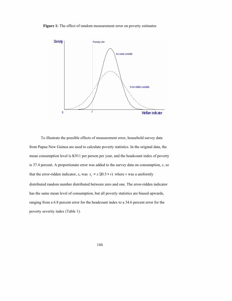
144
Figure 1: The effect of random measurement error on poverty estimates
To illustrate the possible effects of measurement error, household survey data
from Papua New Guinea are used to calculate poverty statistics. In the original data, the
mean consumption level is K911 per person per year, and the headcount index of poverty
is 37.4 percent. A proportionate error was added to the survey data on consumption, x, so
that the error-ridden indicator, xe was (0.5 )ex x v= ⋅ + where v was a uniformly
distributed random number distributed between zero and one. The error-ridden indicator
has the same mean level of consumption, but all poverty statistics are biased upwards,
ranging from a 6.8 percent error for the headcount index to a 34.6 percent error for the
poverty severity index (Table 1).
Welfare indicator
Density Poverty Line
Accurate variable
Error-ridden variable
0 z 0
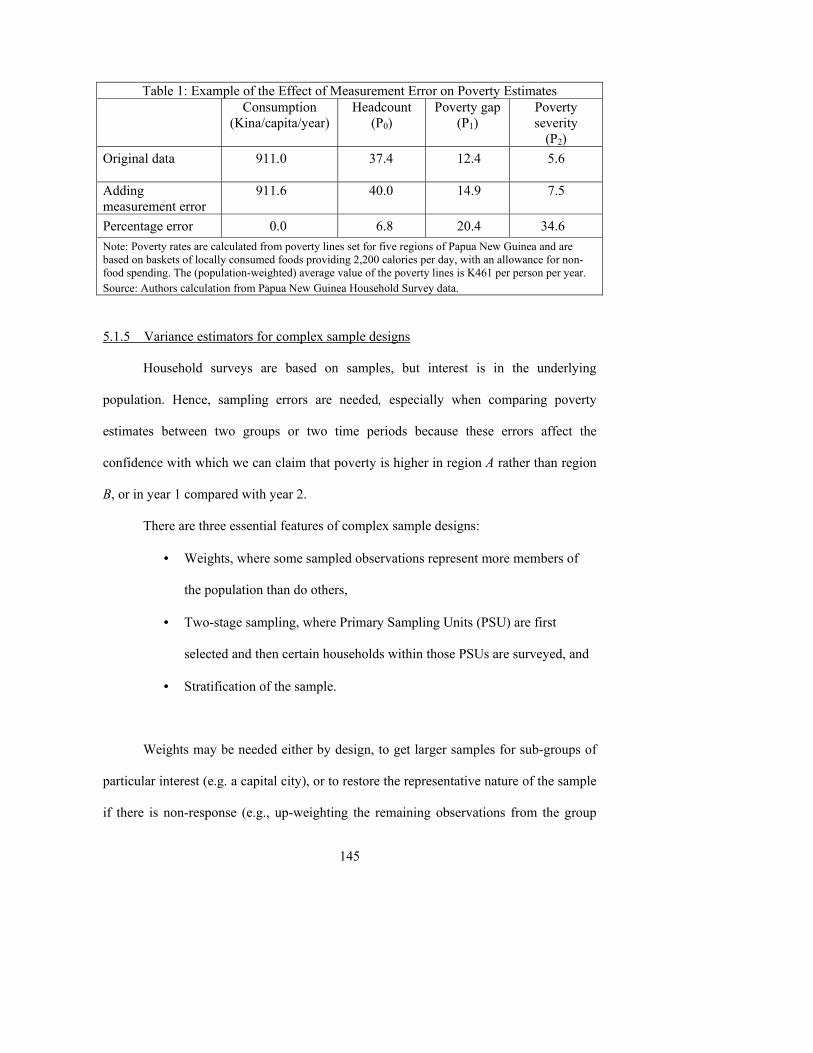
145
Table 1: Example of the Effect of Measurement Error on Poverty Estimates Consumption
(Kina/capita/year) Headcount
(P0) Poverty gap
(P1) Poverty severity
(P2) Original data
911.0 37.4 12.4 5.6
Adding measurement error
911.6 40.0 14.9 7.5
Percentage error 0.0 6.8 20.4 34.6 Note: Poverty rates are calculated from poverty lines set for five regions of Papua New Guinea and are based on baskets of locally consumed foods providing 2,200 calories per day, with an allowance for non-food spending. The (population-weighted) average value of the poverty lines is K461 per person per year. Source: Authors calculation from Papua New Guinea Household Survey data.
5.1.5 Variance estimators for complex sample designs
Household surveys are based on samples, but interest is in the underlying
population. Hence, sampling errors are needed, especially when comparing poverty
estimates between two groups or two time periods because these errors affect the
confidence with which we can claim that poverty is higher in region A rather than region
B, or in year 1 compared with year 2.
There are three essential features of complex sample designs:
• Weights, where some sampled observations represent more members of
the population than do others,
• Two-stage sampling, where Primary Sampling Units (PSU) are first
selected and then certain households within those PSUs are surveyed, and
• Stratification of the sample.
Weights may be needed either by design, to get larger samples for sub-groups of
particular interest (e.g. a capital city), or to restore the representative nature of the sample
if there is non-response (e.g., up-weighting the remaining observations from the group
146
with high non-response rates). Two-stage sampling occurs because it is a cost effective
way of carrying out fieldwork; it is cheaper to get a sample of 100 by visiting just 10
villages and selecting 10 households from each rather than visiting 100 villages and
selecting just one household in each village. Stratification occurs because survey
designers find that if they use prior information on factors that are likely to be associated
with poverty (e.g., geographical remoteness) they can draw a sample in closer accordance
with the proportions in the population rather than leaving this to chance.
Two-stage sampling is less efficient than simple random sampling in statistical
terms (which causes larger standard errors). This is because the households within a PSU
tend to have similar characteristics, so a sample drawn from them reflects less of the
population�s diversity than would a simple random sample with the same number of
households. At the same time, stratification reduces sampling errors because it reduces
the chance that a relevant part of the sampling frame will go unrepresented. Ignoring
these complex design features can considerably bias estimates of sampling error. Howes
and Lanjouw (1998) find the standard error of the headcount poverty rate in Ghana is 45
percent higher when clustering and stratification are accounted for compared with
wrongly assuming simple random sampling.
Techniques for calculating sampling variance and standard errors from complex
sample designs fall into two general categories: Taylor series linearization and replication
techniques. A Taylor series expansion is a linear approximation to a nonlinear function,
and this is relevant because many estimates of interest in sample surveys are nonlinear.
147
Formally, 20 0 0 0 0( ) ( ) ( )( ) ( ) ( ) 2!f x f x f x x x f x x x′ ′′= + − + − +K which says that the
function ( )f x can be approximated at one point, x, by taking its value ( )0( )f x at a
nearby point, 0x , and using the slope at that point, 0( )f x′ , to extrapolate to the point
where we want to evaluate the function.
An improvement in the approximation comes from the second order term
20 0( ) ( ) 2!f x x x′′ − ( f ′′ is the second derivative and ! is the factorial, so 2! is 1 2 2× =
and 3! is 1 2 3 6)× × = and the higher order terms. Variance estimators used with survey
data assume that the second and higher order terms are of negligible size, leaving only the
first-order, linear, portion of the expansion, ( ) [ ]0 0 0var ( ) var ( ) ( )( ) .f x f x f x x x′≈ + − In
other words, the variance estimate for a linear approximation to the estimator is used to
estimate the variance of the estimate itself.
A wide range of software is available to calculate the variance of survey estimates
using this linearization technique. For example, CENVAR within the IMPS package
provided by the US Census Bureau and CSAMPLE within the EPI-INFO package
provided by the US Center for Disease Control use linearization. This is also the main
method used in the survey analysis procedures for general purpose econometric software
like SAS and STATA. Two features of this estimation approach are relevant. First, a
separate formula for the linearized estimate must be developed for each type of statistical
estimator (such as a mean or a ratio). This is not a binding constraint because all of the
widely used poverty measures can be expressed as the mean of a suitably transformed
148
variable. For example, the poverty severity index (P2) is just the mean of the squared
proportionate poverty gaps, [ ]2( )z y z− where z is the poverty line, y is the welfare
indicator, and the squared proportionate gap is zero if .y z≥ 35 The second feature is that
these estimators require at least two PSUs per stratum, which will usually be achieved by
the sample design although it can be violated when examining narrow sub-populations.
Replication techniques take repeated sub-samples, or replicates, from the data.
These replicates are then used to recompute the weighted survey estimates. For example,
50 replicate samples might be drawn from the original sample, and the poverty rate is
calculated from each of these 50 replicates. The variance is then computed in terms of the
deviations of these replicate estimates from the whole-sample estimate. The two main
replication methods are Balanced Repeated Replication and Jackknife Repeated
Replication. The basic idea of jackknife replication can be illustrated for the sample
variance of the mean in a simple random sample. Suppose n=5 and sample values of y are
6, 10, 4, 2, and 8. The sample mean 6,y = and its sampling variance is
( ) 2var( ) 1 ( ) ( 1) 2.iy n y y n= − − =∑ As an alternative to this analytical formula for the
variance, the jackknife variance of the mean is obtained as follows:
1. Compute a pseudo sample mean by deleting the first sample value, which
results in (1) (10 4 2 8) / 4 6.y = + + + = By deleting the second sample value
instead, the second pseudo mean is (2) (6 4 2 8) / 4 5;y = + + + = and similarly,
(3) (4)6.5, 7,y y= = and (5) 5.5.y =
35 Variations in household size and in household sampling weights may require a weighted mean to be used.
149
2. Compute the mean of the five pseudo-values ( )
30 5 6,i
y y n= = =∑ which
is the same as the sample mean, and
3. Estimate the variance from the variability among the five pseudo-values,
[ ] 2( )var( ) ( 1) ( ) 2,iy n n y y= − − =∑ which gives the same result as the
analytical formula above.
Obviously there is no need to use jackknife replication for the variance of the
mean of a simple random sample because an analytical formula is available. But the same
idea can be extended to clustered samples. Specifically, a replicate can be formed by
removing one PSU from a stratum and weighting the remaining PSUs in that stratum to
retain the stratum�s share of the total sample, and a pseudo-value can be estimated from
each replicate. With the Balanced Repeated Replication, the replicates are formed by
dividing each stratum into two PSUs and randomly selecting one of the two PSUs in each
stratum to represent the entire stratum. Clearly, both replication techniques require at
least two PSUs in each stratum.
Fewer software packages appear to use replication techniques compared with
those using the linearization approach. Among those that do are VPLX which is supplied
free by the US Census Bureau and WesVar, while a replication add-on has recently been
made available for STATA.36 The difference in availability of software for the two
methods is unlikely to reflect any belief that one method for dealing with complex sample
36 The linearization method has been available in Stata since version 5 (ca. 1996) under the command prefix svy, while a freely available add-on for the replication methods under the command prefix svr is available at http://econpapers.repec.org/software/bocbocode/s427502.htm
150
date is superior to the other. According to Korn and Graubard (1999), estimators based
on smooth functions of the sample data (e.g., totals, means, proportions, and differences
between proportions) have comparable variance estimates under both replication and
linearization methods.
Regardless of the method used to calculate the sampling variability for complex
samples, obtaining correct variances is especially important in the context of poverty
monitoring. In monitoring, the main interest is the change in poverty levels--if any--
between measurement periods, say t1 and t2. If Yt1 and Yt2 are the poverty statistics, we
would like to know whether the observed difference, Yt2 � Yt1, is indicative of a real
change in the population rather than just reflecting sampling variability. Thus what is
required is an estimate of the variance of the difference: V(Yt2 � Yt1 ) = V(Yt2) + V(Yt1)
� 2 Cov(Yt2,Yt1 ). The terms on the right-hand side can be estimated as design-based
variance estimates of means or of ratio estimates. Let the square root of the resulting
estimate be se(Yt2-Yt1), i.e., the standard error of the difference. The interval, Yt2 � Yt1 ±
1.96 se(Yt2 � Yt1 ) defines a 95 percent confidence interval about the true difference (it
would be 90 percent if 1.64 were used instead of 1.96). A confidence interval that is to
the left of zero is indicative of an increased poverty rate. One that captures zero supports
a �no change� hypothesis. An interval to the right of zero provides empirical evidence
for a reduced poverty rate.
Under normal conditions wherein the poverty situation changes slowly, the real
difference in poverty incidence narrows as the interval between t2 and t1 is shortened. This
151
means a commensurately very small standard error is required to detect a small change in
the poverty incidence for the population. Thus, more frequent monitoring does not mean
a smaller sample size for each survey round. On the contrary, a more efficient sampling
design and bigger sample are needed to reduce the noise (sampling error) to a level that
would provide a good chance of detecting a weak signal (change in poverty incidence).
Otherwise, there would be no point in the monitoring exercise if it were known a priori
that the computed confidence interval will most likely straddle zero. It is to be noted also
that all these considerations, including sample size, pertain equally if not more to sub-
national domains of interest, e.g., urban-rural and regions, rather than to national level
estimates.
5.2 Types of surveys
Several different types of household survey can be used to measure and analyze
poverty. Very few of these surveys have poverty measurement as their primary objective.
Thus statistical agencies have to carefully evaluate whether surveys that have other (or
multiple) objectives can provide reliable data for measuring poverty.
5.2.1 Income and expenditure (or budget) surveys
Almost all countries have either a Household Income and Expenditure Survey
(HIES) or a Household Budget Survey (HBS). Methods used to measure consumption
expenditures in these surveys vary widely, in terms of data collection (recall, family
diaries, and individual diaries), reference periods over which consumption is observed,
152
and whether households are observed only once or revisited during a year. But one
common feature is that in almost all cases the HIES and HBS are designed mainly to
provide expenditure weights for a Consumer Price Index (CPI) and to assist in the
calculation of National Accounts. For these tasks a survey only needs to provide
estimates of means and totals. But there are important differences between the needs of
CPI-focused and poverty-focused surveys, involving topical coverage, reference periods,
and the need for revisits. Consequently, if statistical agencies are to place more weight on
the objective of improving poverty measurement, certain changes to the design of these
surveys may be warranted. An immediate problem in using HIES and HBS for poverty
analysis is that because of the burden of remembering expenditures on so many items,
respondents are typically asked about few other topics. Thus, there are often few
variables available from the survey that can either help explain the poverty status of the
household or assist in the more general objective of modelling household behaviour.
In contrast, poverty-focused surveys typically obtain measures of total
consumption that do not have the level of commodity detail sought in an HIES or HBS.
The reduced effort spent gathering the consumption data allows more attention to be paid
to a broader array of topics that can assist in modelling the effect of various anti-poverty
interventions. One key topic needed for poverty-focussed surveys is local prices which
are rarely collected by HIES and HBS. Section 5.3 discusses this fully.
Although poverty-focused surveys do not need a lot of commodity detail, they do
have to provide an accurate estimate of long-run welfare for each household in the
153
sample. Such accurate estimation at the household level is not required for surveys that
focus only on population means and totals because the effects of random errors can be
expected to cancel each other out in the estimation of the mean. But for poverty rates and
other variance-based statistics, the effect of random errors accumulates so errors in
measuring household level welfare will be reflected in inaccurate estimates of aggregate
poverty rates.
While the limited topical coverage of HIES and HBS restricts poverty analysis,
the major problem with these surveys is the short period over which consumption is
observed. Because respondents find it hard to remember spending on frequent purchases,
HIES and HBS typically use a very short reference period (e.g., a one-week recall or a
two-week diary), which may be atypical of the household�s usual standard of living. This
short observation period is sufficient if the goal is just to measure the average shares of
household expenditure devoted to each good and service, which is all that CPI
expenditure weights are. Specifically, if the sample is spread evenly over the months in
the year, it is possible to get an annual average for a synthetic �representative household�
without accurately estimating the annual expenditures of each household. In contrast,
poverty measurement requires accurate estimates of long-run welfare for each household.
Such long-run measures appear to be provided by some surveys that report
expenditures and poverty on an annual basis. But many of these surveys simply observe
households for a week, fortnight, or month, with consumption from these periods
annualised by multiplying by 52, 26, or 12. The length of the reference period may vary
154
with the category of consumption, being longer for costly and/or infrequently consumed
items and shorter for frequently consumed and minor items that would be easily
forgotten. While the scaling factors that convert these short duration observations into
annual figures vary, the principle in all cases is the same: an estimate of annual
expenditures can be made by simple extrapolation from shorter observation periods.
What is the problem with these annualised estimates and also with estimates that
are collected and reported for shorter periods like a fortnight or a month? Random
shocks, which occur during the observation period and are subsequently evened out over
the rest of the year, get included along with the genuine between-household inequality in
annual expenditures. Consequently, estimates of annual inequality are overstated. In any
setting where the poverty line is below the modal value of per capita expenditure, the
overstated dispersion will also lead to an overstatement of the poverty head-count and
other measures of poverty.
The degree to which measured annual inequality and poverty are overstated when
short reference periods are used can be seen in urban China (Table 2). China is of interest
in this regard because respondents in the HIES in China keep a daily expenditure diary
for a full 12-month period, which provides a benchmark to evaluate estimates that are
based on extrapolations from shorter periods. For example, if expenditures for each
household were only observed for one month (but the sample is spread over the year) and
multiplied by 12 to give an annualised estimate, inequality in annual expenditures would
be overstated by over 60 percent, annual headcount poverty by over 50 percent, and the

155
poverty gap index by 150 percent.
The upward bias is roughly halved if expenditures are annualised from two
months of data (collected six months apart) and declines further if the survey collects
either four or six months of expenditure data. It is notable that there is no overstatement
in estimates of mean annual expenditure when any of the short-period data are
extrapolated to annual totals. This emphasises the fact that a survey design that does a
good job of estimating the mean will not necessarily be accurate for variance-based
measures like poverty and inequality.
Table 2: Percentage Overstatement in Inequality and Poverty Measures for Urban China when Annual Expenditures are Obtained by Extrapolating from Monthly Data
Extrapolation based on observations in: 1 month 2 months 4 months 6 months
Corrected extrapolation
Mean annual expenditure
0.1 0.1 0.1 0.1 0.1
Gini index of inequality
64.6 36.4 17.7 11.6 6.4
Head-count poverty rate
53.1 32.2 14.0 15.0 0.1
Poverty gap index 149.8 77.8 34.2 19.4 5.0 Note: Corrected extrapolation uses correlation from a single revisit (i.e., two months of data). Source: Gibson, Huang and Rozelle (2003).
One response to exaggerated poverty estimates that come from extrapolated
annual expenditures is to only report poverty for shorter periods, corresponding to the
reference period used by the HIES. For example, if a survey observes most household
consumption for only a week, the poverty estimates would also be reported on a weekly
basis. However, such short-period estimates may be dominated by transitory fluctuations.
156
Cross-country comparisons will also be difficult unless a standard reference period is
agreed to, although this problem already exists because extrapolated annual estimates are
not comparable to proper annual data like those available from China. Annual reporting
periods are likely to continue to be used while agriculture remains an important source of
household income because of the resulting seasonality in consumption and poverty.
5.2.2 Correcting overstated annual poverty from short reference period HIES and HBS data
One method that may combine the practicality of short observation periods with
the need for annual estimates of expenditures and poverty is to revisit some surveyed
households at least once during a year. Rather than simply adding the two estimates of
the household�s expenditure and naively extrapolating to an annual total (as was done in
Table 2), Scott (1992) suggests a �corrected extrapolation� based on correlations
between the same household�s expenditures in different periods of the year � correlations
implicitly assumed to be 1.0 by simple extrapolation.
For example, consider a survey that gathers all expenditure data using a one-
month reference period (as the National Sample Survey in India did until recently). Let
xm refer to the average, and V(xm) the variance, of monthly expenditures across all i
households and t months in the year. Extrapolating to annual expenditure totals by
multiplying monthly expenditures by 12 gives an estimated variance of annual
expenditures of 144⋅V(xm). As indicated in Table 2, this extrapolation overstates the
157
variance in the annual expenditures that would be recorded if each household was
observed for a full 12-month period:
( ) )4(1)(2
1,∑
=
−=N
iaaia xxx N
V
where aix , is annual expenditure by the ith household and xa is average annual
expenditures. Equation (4) can be expressed as:
)5()(12
1','',∑
=
=tt
tttta rxV σσ
where rt,t� is the correlation between expenditures in month t and month t ′ and tσ is the
standard deviation across households in month t. This follows because xx aai −, in
equation (4) can be expressed as the sum of the deviations of each household�s monthly
expenditure from the mean for that month, xxd titit −= and the dit terms are components
of the correlation coefficient:
)6(.1'
1'', σσ tt
N
iitittt ddr N ∑=
=
Assuming that the dispersion across households does not vary from month to month,
tt ′=σσ,i.e. equation (5) can be expressed as:
[ ] )7(.)(13212)( xma VrxV ⋅+=
where r is the average correlation between the same household�s expenditures in all pairs
of months in the year. Equation (7) shows that the variance from simple extrapolation to
annual totals, 144⋅V(xm), equals V(xa) only in the special case of 1=r .
158
The corrected extrapolation uses estimates of r to scale the ith household�s
deviation from the overall monthly average )( xxit m− , up to an annual value. Adding this
to the annual average across all households, ,12 ma xx ⋅= gives:
( ) )8(.1213212, xxx mmitAi rx ⋅+⋅+−=
For example, if 0.5,r = the scaling factor is only 8.8 (=√78), rather than the scaling
factor of 12 implied by simple extrapolation. Thus, the deviation of a household�s
one-month expenditures from xm has a smaller effect than under simple extrapolation,
leading to a less dispersed distribution of annual expenditures and a lower poverty
estimate (if the poverty line is below the mode of the expenditure distribution).
While the most reliable estimate of r would use the 66 correlation coefficients
rt,t� between all i≠j pairs of months, this provides no practical advantage because it
requires observing each household in every month in the year, as is done, for example, by
the HIES in China. However, even getting an estimate of r from just two, non-adjacent
months may be sufficient.
The final column of Table 2 shows that this method gives estimates that are quite
close to those obtained from observing each household�s expenditure for all 12 months of
the year. In urban China, the errors from this corrected extrapolation method never
exceed 6 percent and are much smaller than the errors generated by multiplying monthly
data by 12, as was done in the first column of Table 2. Using revisits in more months to
form a more reliable estimate of r does not significantly improve estimates (Gibson et
al., 2003).
159
Thus, a single revisit about six months after the first survey of the household�s
expenditure may give a good estimate of r so that equation (8) can be used to improve
estimates of annual poverty, even when a HIES or HBS uses short observation periods.
This economical approach to estimating r will be valid if the correlations among non-
adjacent periods vary little as the gap between observations increases, as was found by
the 1993-94 Household Budget Survey in Zambia where rt,t′ fell by just 0.0078 for each
month that the gap between t and t′ increased (CSO, 1995).
Further savings may be made by restricting the repeated observations to a random
subset of the sampled households to lessen the cost of getting the parameter .r This
random sub-sample should be large enough to allow r to be calculated separately for
major groups of the population (e.g., rural and urban, and rich and poor) because the
extent to which expenditures fluctuate within the year may differ between these groups.
For example, in a survey in Papua New Guinea, households in 20 percent of the primary
sampling units in the sample were revisited about six months after the initial survey to
estimate ,r and this only added about 10 percent to the cost of the survey (compared
with just using a cross-section) while substantially improving poverty estimates (Gibson,
2001).
5.2.3 Living Standards Measurement Study surveys
In contrast to the HIES and HBS, both of whose main objective is to measure
means and totals, the Living Standards Measurement Study (LSMS) surveys of the World
Bank have a primary focus on measuring the distribution of living standards.
160
Consequently, the design of the LSMS has been dictated by the need to have accurate
measures of monetary living standards for each household in the sample, not just for a
representative household. Even though the LSMS surveys collect information on both
income and consumption, poverty measurements from these surveys have always used
consumption data. In contrast, some analysts choose to measure poverty using income
data from HIES, even when consumption expenditure data may be available.
A further difference is that the LSMS surveys are explicitly multi-topic surveys.
In addition to income and consumption, they collect detailed data on education, health
and anthropometry, employment, migration, agriculture, non-farm enterprises, savings
and credit, and community-level data on public services and local prices. This more
extensive coverage is achieved by reducing the commodity detail required in the
consumption module.
Besides providing alternative indicators of poverty (such as lack of education,
poor access to water, and malnutrition of children), the broader topic coverage of LSMS
surveys enables household behaviour to be modelled. This can help in the formation of
policies to break the intergenerational cycle of poverty (Box 3). For example, households
where adults have low levels of education tend to be poor. Hence, LSMS surveys include
considerable detail on educational expenses, distance to schools, and quality of school
materials for current students. These data can help explain factors that limit enrollment of
certain groups of students (e.g., girls, and students from particular regions or income
groups). Once those factors are identified, interventions can be designed to improve
161
current enrollments and reduce the likelihood of future poverty.
Box3: Mother�s Education, Child Stunting, and Intergenerational Poverty in Papua New Guinea.
Analyses of LSMS survey data from Papua New Guinea have identified one mechanism through which poverty and ill-health are transmitted across generations and suggests an intervention that could break this cycle (Gibson, 1999). The low levels of education of mothers compared with fathers (a gap of two school years, on average) contributes to the stunted growth of children (i.e., children are shorter for their age). Parental education affects stunting by improving knowledge of health and nutrition, as well as by increasing incomes. In fact, an additional year of schooling for mothers is three times more effective at reducing stunting than is a year of schooling for the father (with or without controls for income). Stunting matters to poverty because stunted children have higher risk of sickness and death and poorer mental development. In addition, stunted girls grow up to be stunted mothers, who are more likely to give birth to underweight babies that have a greater risk of being stunted (UNICEF, 1998). Hence, the vicious circle, caused partially by gender bias in schooling, continues across generations.
A very detailed description of all modules in the LSMS surveys is available in
Grosh and Glewwe (2000). The most important module from the point of view of poverty
measurement is the consumption module, fully described by Deaton and Grosh (2000).
Only two aspects of LSMS surveys are considered here: use of bounded recall and use of
recall questions designed to provide information for an annual reference period.
To prevent telescoping errors, which are a mis-dating of expenditures, some
LSMS surveys used a bounded recall where interviewers first visited respondents to
administer modules of the survey other than the consumption recall. A subsequent visit
was then made one or two weeks later and respondents were asked about consumption
162
since the previous visit. The expectation was that the initial visit would clearly mark the
beginning of the recall period and reduce the mis-dating of consumption. There does not
appear to have been an evaluation of this design, although it was consistent with findings
in the literature on telescoping (Neter and Waksberg, 1964), and it was not used in all
LSMS surveys, creating some non-comparability.
In addition to either a bounded or unbounded recall of consumption over an
immediately previous period like a month, some LSMS surveys attempted a longer term
recall. Following a screening question on whether the household consumed the particular
item during the past year, respondents who had were asked about the number of months
they purchased the item, the number of times per month they purchased the item, and the
usual quantity and value of this usual purchase. A similar set of questions was asked
about own-production and other non-purchases (such as gifts received). The product of
usual purchase value, times per month usually purchased, and months per year purchased
may give an estimate of annual expenditure on the item.
If these questions are answered accurately they solve the problem of overstated
inequality and poverty when annualizing consumption estimates from short reference
periods. Deaton and Grosh (2000) present evidence that suggests this form of annual
recall provides similar data to recall over the previous month. However, this is not a firm
verification because the two types of data are gathered in the same interview and are
likely influenced by each other. This is an area where statistical agencies could usefully
carry out further experiments.
163
5.2.4 Core and module designs
While multi-topic surveys are useful for poverty measurement and distributional
analysis, they are hard to conduct. Therefore, data are normally available only at low
frequency and for small samples, making them less useful for poverty monitoring. Some
statistical agencies deal with this problem by using a core-module design. A simple core
survey is fielded frequently and a variety of rotating modules are appended to the core
survey. For example, the Indonesian SUSENAS has an annual core with questions on
demography, education, labour market activity, and an abbreviated consumption recall
that covers 23 broad categories. This is supplemented with a detailed consumption
module, using 320 detailed categories, that is given to a subset of respondents every third
year. In the intervening years, modules on other topics are used.
Although the core-module design is popular, it has at least two drawbacks that can
cause inconsistent poverty comparisons. First, estimates from detailed consumption
modules are often inconsistent with the results from abbreviated consumption questions
in a core. For example, in SUSENAS the consumption estimates in the core appear to be
understated, particularly for households with higher true consumption (mean reverting
error) and for larger households (Pradhan, 2001). It is therefore not possible to create a
consistent annual series of consumption and poverty estimates by using results from the
core survey in two years and from the module survey in the third year. Second, contents
of rotating modules can affect the core so even core-to-core temporal comparisons may
be inconsistent. For example, in the Cambodia Socio-Economic Survey (CSES) of 1999,
164
the addition of a detailed income module affected the consumption data in the core
because of a desire by either respondents or interviewers to reconcile consumption and
income at the household level (see Box 2).
The behaviour of poverty analysts can also be affected by the contents of a
module. A detailed social sector module in the 1997 CSES had estimates of health
expenditures that were much higher than the health spending recorded in the core, so the
estimate of total expenditure for the core survey was adjusted higher (by up to 14
percent) because of the presumed undercount. This destroyed the comparability with
consumption and poverty estimates from previous and subsequent core surveys where
this adjustment had not been made (Gibson, 2000). These examples suggest that care is
needed in the use of core-module surveys.
5.2.5 Demographic and Health Surveys
Demographic and Health Surveys (DHS) now cover more than 170 surveys in 70
countries throughout the developing world. Country-specific details of these surveys can
be found at www.measuredhs.com. A somewhat similar, though less well known set of
surveys, are the Multiple Indicator Cluster Surveys (MICS) that are carried out by
UNICEF. These surveys have three potential advantages over more traditional sources of
household data for poverty analysis.
• They are available for a wider range of countries, especially in Africa;
• In many countries they are available at two or more points in time,
allowing temporal comparisons; and
165
• Key survey instruments are standardized for all countries so cross-country
comparability is much greater than in any other type of household survey.
Offsetting these potential advantages, a very major drawback of DHS and MICS
is that, except for a few experimental modules, they do not collect information on either
incomes or consumption. Consequently it is not possible to use this rich source of data for
conventional poverty measurements. However, recent research suggests that the
information collected by these surveys on dwelling facilities (e.g., presence of piped
drinking water) and asset ownership (e.g., radios and bicycles) may provide a measure of
household economic status that may be useful for distributional and poverty analysis.
There are two lines of this research, only one of which has proceeded directly to poverty
measurement. The most well known statistical method for using these surveys in place of
consumption data is based on research by Filmer and Pritchett (2001). These authors use both
household consumption expenditure and an �asset index� to see which is better at explaining
patterns of children�s school enrollments in Nepal, Indonesia, Pakistan, and states of India (using
the National Family Health Survey for India, which is similar to the DHS). They find that the
asset index is a proxy for economic status that is at least as reliable as conventionally measured
consumption expenditures. This asset index uses the method of principal components, which is a
mathematical technique for transforming several correlated variables (on household asset
ownership and dwelling facilities in this case) into a smaller number of uncorrelated variables.
Only the first principal component, which accounts for as much of the variability in the data as
possible, is used by Filmer and Pritchett (2001) and others who follow their approach. Typically
166
this component accounts for about 25 percent of the variation in asset ownership and facilities in
a DHS. There are no units for interpreting this asset index, so it is used only for ordinal
comparisons. One common use has been to compare educational attainment of the richest 20
percent of households and the poorest 40 percent (see
http://www.worldbank.org/research/projects/edattain/edattain.htm).
While the asset index approach of Filmer and Pritchett (2001) has not been used
to directly study poverty, a related method has been developed by Sahn and Stifel (2000)
to make poverty comparisons across time and space for 11 African countries. In this
method, DHS data from all 11 countries are pooled and an asset index is formed using the
method of factor analysis. Unlike the method of principal components, which uses all the
variability in an item, factor analysis allows some variability to be unique, with only the
variability that is common with the other items used to form the asset index.
Relative �poverty lines� are created from the asset index, based on the values of
the index at the 25th and 40th percentile of the pooled sample. Poverty comparisons are
made across countries, and especially over time for each of these countries by seeing
what proportion of the population in a subsequent DHS have an asset index that is below
the values that were at the 25th and 40th percentiles in the first survey. The change in
poverty over time is also calculated with the poverty gap and squared poverty gap
measures, and this change is decomposed by sector.
There would need to be a validation of this method to see whether the results
167
closely mimic those calculated with more typical consumption data before any
recommendations could be made about its wider use. Even in the absence of such a
validation, there are at least three concerns with the approach:
• An index based on the principal components approach (and presumably also
the factor analysis approach) appears to put higher weights on durable goods
that are easier to own which is not the pattern that occurs for an index based
on a more explicit model for the ownership of durables (Mukherjee, 2005);
• The link between assets and expenditures is likely to be non-linear, so the
ability of an asset index to serve as a proxy for unmeasured consumption is
likely to vary over the income distribution and through time; and
• The very simplicity of the questions that underlie the asset index could also
prove to be a weakness because yes/no questions on ownership of an asset do
not distinguish between the wide variations in quality of these assets.
5.3 Pricing and updating the value of poverty lines
Information on the prices that households pay for items they consume is crucial
for poverty measurement. Most obviously these prices are needed to place a monetary
value on the food basket for a Cost of Basic Needs (CBN) poverty line. Prices are also
needed to calculate the change over time in the cost of reaching a poverty line standard of
living. Even methods for constructing a poverty line that seem to rule out the need for
prices, such as the Food Energy Intake (FEI) method, prove on further examination to
168
require information on prices.37 In fact, measurement of local prices is needed for some
or all of the following three tasks:
1. pricing the food basket for the Cost of Basic Needs (CBN) poverty line,
2. forming spatial deflators, so that any ranking of household consumption
expenditures is in real rather than nominal terms, and
3. imputing values either when the survey only collects quantities or when
checking the sensitivity of the consumption estimates to the use of respondent-
reported values.
The methods used to calculate a CBN poverty line are discussed in Chapter 4 so
attention here is restricted to the calculation of spatial price deflators and the use of price
data for imputing values when only quantities are collected.
5.3.1 Spatial price deflators Spatial price deflators are needed because price differences between regions may
make between-household comparisons of nominal consumption expenditures
misleading.38 For example, in the CBN method of setting poverty lines it is typical to base
the poverty line basket of foods on the actual consumption pattern of a group of poor
37 The FEI method relies on a regression of calorie intakes on a welfare indicator like per capita expenditures. Once a calorie target is set (say, 2000 calories per person per day) the regression is inverted to solve for the required expenditure to meet the calorie target. However there will be a measurement error in this regression if it is carried out in terms of nominal expenditures when there are large price differences between regions. This error will tend to reduce the magnitude of the regression coefficient, causing an overstatement in the level of expenditures required to reach the calorie threshold and hence an overstatement in the value of the poverty line. This error could be reduced if price data were available to calculate real expenditures that reflect regional differences in the cost of living. 38 Temporal price deflators may also be needed. It is typically assumed that prices do not vary over time within a cross-section but in inflationary environments even a few months between the time of the first and last household being surveyed could cause a difference between nominal and real expenditures.
169
households.39 But in order to identify this group of poor households, some ranking must
be used and this needs to control for spatial price variation. Otherwise poor households
from regions where prices are high are less likely to be included in the reference group
than are poor households in regions where prices are low because those from the higher
priced region will have higher nominal expenditures.
The ideal way to control for spatial differences in the prices facing households is
to calculate a �true cost-of-living index�. This true cost-of-living index is based on the
expenditure function, ( )c c u= , p , which gives the minimum cost, c for a household to
reach utility level u when facing the set of prices represented by the vector p. For two,
otherwise identical households, one living in the base region and facing prices p0, and the
other living in another region facing prices p1, the true cost-of-living index is:
( )( )True cost - of - living index =
c u
c u
,
,
1
0
p
p
which can be interpreted as the relative price in each region of a fixed level of utility.
Although this is the ideal spatial price index, it is not commonly calculated, even in
developed countries.
Instead the usual approach to controlling for spatial price differences is to use a
price index formula that approximates the true cost-of-living index. A common choice is
39 Exactly how many households should be in this group depends on prior notions of the poverty rate. For example, if it was believed that the poverty rate was 0.25 it would be likely that an analyst would use the food consumption patterns of the poorest quarter of households for obtaining the poverty line basket of foods. If this prior estimate of the poverty rate turns out to be quite different than the subsequently calculated one, it may be necessary to revise the calculations, using a different definition of the starting group (Pradhan, Suryahadi, Sumarto and Pritchett, 2001).
170
the Laspeyre�s index, which calculates the relative cost in each region of buying the base
region�s basket of goods:
PQ
PQ
kj
J
jkj
ij
J
jkj
L∑
∑
=
==
1
1 ,
where k is the base region, i indexes every other region, j indexes each item in the
consumption basket, and Q and P are quantities and prices.
The Laspeyre�s index overstates the cost-of-living in high price regions. It does
not let households make economising substitutions away from items that are more
expensive in their home region than they are in the base region. For example, ocean fish
are usually more expensive in the interior of a country than on the coast, so the quantity
of fish consumed would typically be lower in the interior than on the coast. But if a
coastal region is the base region, the Laspeyre�s index calculates the cost of purchasing
the coastal level of fish consumption at the high prices prevailing in the interior. Instead,
a true cost-of-living index would calculate the cost of obtaining the coastal level of utility
when facing the high prices for fish that prevail in the interior, letting the household
rearrange its consumption bundle to minimise cost.
Another commonly used price index, the Paasche index understates the cost of
living in high price regions because it evaluates relative prices using a basket of goods
that varies for each of the i regions:
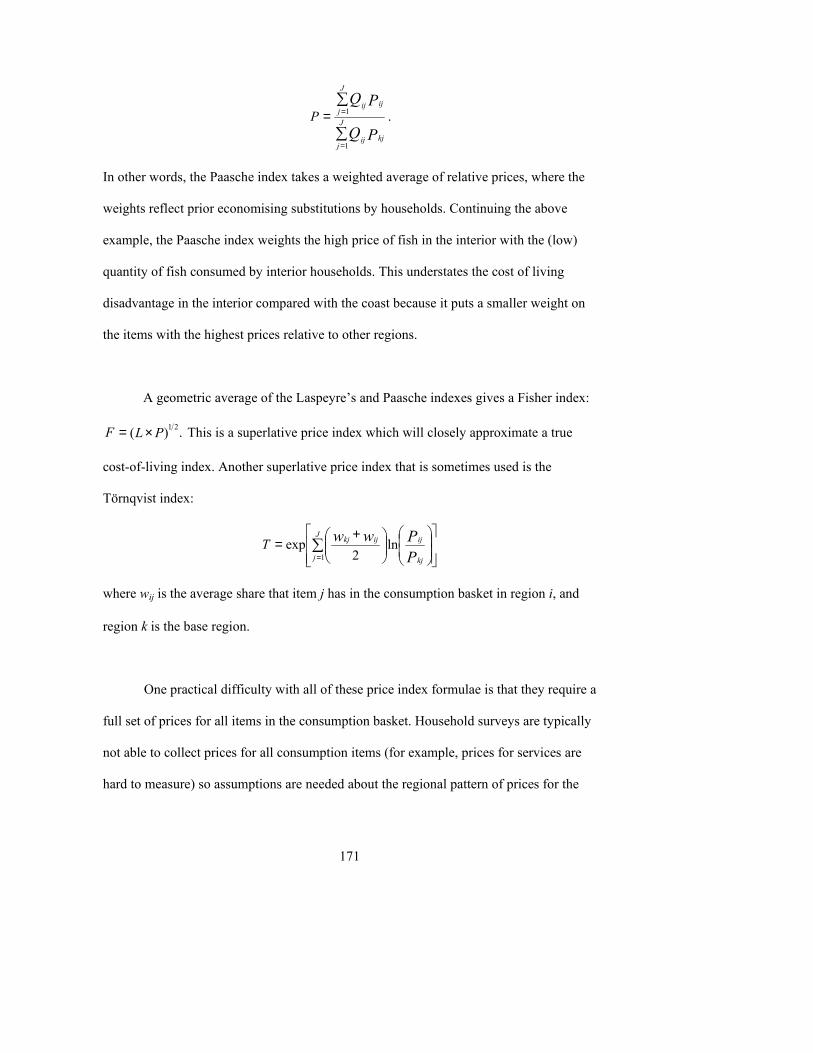
171
PQ
PQ
kj
J
jij
ij
J
jij
P∑
∑
=
==
1
1 .
In other words, the Paasche index takes a weighted average of relative prices, where the
weights reflect prior economising substitutions by households. Continuing the above
example, the Paasche index weights the high price of fish in the interior with the (low)
quantity of fish consumed by interior households. This understates the cost of living
disadvantage in the interior compared with the coast because it puts a smaller weight on
the items with the highest prices relative to other regions.
A geometric average of the Laspeyre�s and Paasche indexes gives a Fisher index:
.)( 21PLF ×= This is a superlative price index which will closely approximate a true
cost-of-living index. Another superlative price index that is sometimes used is the
Törnqvist index:
+= ∑
= PPww
kj
ijJ
j
ijkjT ln2
exp1
where wij is the average share that item j has in the consumption basket in region i, and
region k is the base region.
One practical difficulty with all of these price index formulae is that they require a
full set of prices for all items in the consumption basket. Household surveys are typically
not able to collect prices for all consumption items (for example, prices for services are
hard to measure) so assumptions are needed about the regional pattern of prices for the
172
items that are not observed. One solution to this problem is to derive the spatial price
index from the regional poverty lines because poverty lines can be calculated when there
are missing non-food prices (see equation (1)). But even for consumption items where it
is conceptually possible to gather price data, there are often practical difficulties that
result in very many missing prices. For example, a 1999 survey in Cambodia tried to
obtain prices for 50 food items in 600 villages but data were obtained on less than half of
the price-village combinations because of items missing from markets (Gibson, 2000).
5.3.2 Whose cost of living? The possibility of deriving a spatial price index from regional poverty lines raises
the important issue of whose cost of living is being measured by the price index. A price
index derived from poverty lines would typically measure regional differences in the cost
of living amongst the poorest x percent of the population, where x is either the fraction of
the population below the poverty line or the fraction whose food budgets were used to
create the poverty line food basket. The regional pattern of cost of living differences for
this group could be quite different to the pattern shown by a price index that places
greatest weight on households who are either in the middle or the upper parts of the
income distribution.
There are three sources of possible difference between a price index for the poor
(such as one derived from a set of regional poverty lines) and a more general purpose
price index that reflects the cost of living for the middle or upper parts of the income
distribution:
173
1. the composition of household budgets changes when moving up the income
distribution, so a price index for the poor would put more weight on basic
necessities,
2. for a given category of consumption (say, rice) the particular brands, grades,
varieties and outlets where rich and poor purchase may differ and also may have
different prices, and
3. various formulae that combine price data with information on the importance of
each commodity in household budgets can place more weight on either rich
households or poorer households.
This question of weighting matters because, as shown above, a price index is
essentially a weighted average of relative prices where the weights reflect the average
importance of the commodity in household budgets. One way to calculate this average
importance for a commodity would be to add up expenditure on that item across all
households, and then calculate the ratio of the total expenditure on that item to the total
expenditure on all items. This is the approach used in the calculation of Consumer Price
Indexes around the world. One feature of this method is that it gives more weight to the
rich, because they have more total spending. Consequently the resulting price index is
sometimes called a �plutocratic price index� (Prais, 1958).
Rather than taking ratios of total spending, another method of calculating the
average importance of a commodity would be to first calculate budget shares for each
household. In the second step these budget shares would be averaged across all
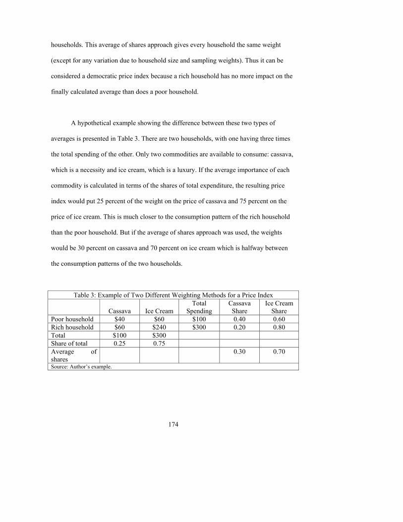
174
households. This average of shares approach gives every household the same weight
(except for any variation due to household size and sampling weights). Thus it can be
considered a democratic price index because a rich household has no more impact on the
finally calculated average than does a poor household.
A hypothetical example showing the difference between these two types of
averages is presented in Table 3. There are two households, with one having three times
the total spending of the other. Only two commodities are available to consume: cassava,
which is a necessity and ice cream, which is a luxury. If the average importance of each
commodity is calculated in terms of the shares of total expenditure, the resulting price
index would put 25 percent of the weight on the price of cassava and 75 percent on the
price of ice cream. This is much closer to the consumption pattern of the rich household
than the poor household. But if the average of shares approach was used, the weights
would be 30 percent on cassava and 70 percent on ice cream which is halfway between
the consumption patterns of the two households.
Table 3: Example of Two Different Weighting Methods for a Price Index
Cassava
Ice Cream Total
Spending Cassava
Share Ice Cream
Share Poor household $40 $60 $100 0.40 0.60 Rich household $60 $240 $300 0.20 0.80 Total $100 $300 Share of total 0.25 0.75 Average of shares
0.30 0.70
Source: Author�s example.
175
There is one other implication of the result that a typical Consumer Price Index uses
weights that are closer to the consumption patterns of rich households. To the extent that
the price trends for items consumed by the rich differ from the trends of those consumed
by the poor, a CPI may be a poor choice for updating poverty lines to account for price
changes over time.
5.3.3 Using prices to impute the value of consumption Self-produced items, and especially food, are a major component of consumption
in rural areas of many developing countries. The monetary values placed on these self-
produced items in surveys are often the values that respondents themselves suggest.
There are grounds for questioning the reliability of these respondent-reported values.
Many households who produce a food do not buy that same food, so they may not be well
informed about prices when they assign a value to their own food production. Moreover,
the items available for sale in markets may be of a different quality than their own
production so even if they are aware of prices in the market they may not be able to
accurately impute a value for their own production.
There are two concerns about relying on respondent-reported values for self-
production. First, they introduce an additional, and extraneous, source of inequality into
measured consumption. If the poverty line is below the mode of the welfare indicator,
this increase in measured inequality will raise the measured poverty rate (see Figure 1).
For example, it may seem unreasonable that two households, who produce the same
quantity of a food in the same location, can value that production differently. A
176
household might fall below the poverty line just by being too pessimistic when valuing
their own food production because they think prices are lower than they truly are.
Second, the values applied to self-produced food items could differ,
systematically, from market prices. Such discrepancies could drive a wedge between the
market prices used to form a Cost of Basic Needs food poverty line and the values used
to form estimates of consumption. If respondents tend to report values for their self-
produced foods that are lower than market prices, estimates of the incidence of poverty
could be inflated, especially in rural areas where subsistence food production is
important.
There are two alternatives to respondent-reported values, as measures of the value
of self-produced food items. The first is to value self-produced foods with the average of
the implicit unit values used by other households in the same cluster (that is, Primary
Sampling Unit) as the respondent. These implicit unit values are the ratio of value to
quantity reported by each respondent, and are similar to a price except that they may
reflect quality variation and also measurement error. Replacing respondent-reported
values with a cluster average removes the within-cluster variability in valuations.
However, it does not address any discrepancy between these average unit values and
market prices which may drive a wedge between the prices used for the poverty line and
the implicit prices used when valuing consumption.
177
The second alternative is feasible only if a survey has collected prices from local
markets. In this case it is possible to value self-produced foods with the average price that
was observed during the survey in the market closest to the respondent. It is notable that
both of these alternative ways of valuing self-produced foods switch the cornerstone of
consumption measurements from the respondent reports of values to the survey estimates
of food production quantities. This does place a lot of faith in quantity measurements, and
these measurements are not necessarily the ones where statistical offices have the greatest
expertise, compared to, say, agriculture ministries and others who do crop surveys. But
unless statistical offices collect prices in local markets it is impossible to know how
sensitive the estimates of consumption and poverty are to the various assumptions made
when valuing self-produced items.
5.3.4 Practical issues in collecting price data Once a decision has been made to obtain price data, either for setting the food
poverty line, calculating a spatial price deflator or placing a value on non-purchased
consumption, there are three practical questions that a statistical agency must consider:
1. How many prices to collect, in terms of the number of items and the number of
individual price observations per item,
2. Where to collect prices, and at what geographical scale to calculate and report
any resulting price indexes, and
3. How to collect the price information, in terms of the following four choices:
178
a. Unit values (that is, the ratio of expenditure to quantity) coming typically
from a consumption recall but potentially also from individual transaction
records in expenditure diaries,
b. Price surveys in community markets, such as those typically done by
LSMS surveys,
c. Surveys of opinions about prices from either sampled households or
community leaders, and
d. Existing price collection efforts, as might already be occurring for a
Consumer Price Index.
In terms of the number of items to collect prices for, ideally there should be full
coverage of all of items in the poverty line (if it is a CBN line with a specified basket of
food) and all of the items specified in the consumption recall (if diaries are not used).
The prices of key non-foods should also be collected even if an Engel method is used to
scale the food poverty line up to the total poverty line (see equation (1)) without using
any non-food prices.
This recommendation for the number of items to collect prices for switches
attention to the issue of how many items to specify in a food poverty line (and the related
issue of how disaggregated are the commodities in the expenditure questionnaire). One
useful tool in this regard is the concentration curve for the foods in the poverty line
basket. This curve starts with the most important food and plots the cumulative
contribution to either the total cost or the total calorie content of the poverty line basket.
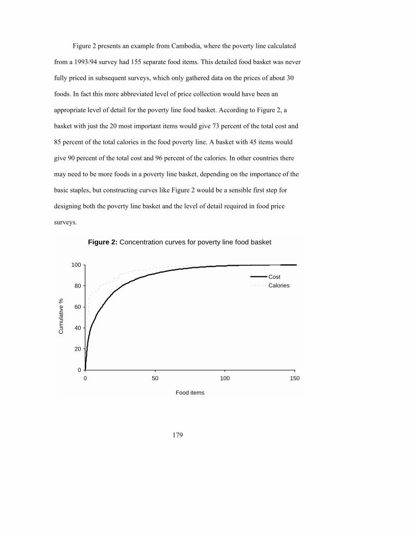
179
Figure 2 presents an example from Cambodia, where the poverty line calculated
from a 1993/94 survey had 155 separate food items. This detailed food basket was never
fully priced in subsequent surveys, which only gathered data on the prices of about 30
foods. In fact this more abbreviated level of price collection would have been an
appropriate level of detail for the poverty line food basket. According to Figure 2, a
basket with just the 20 most important items would give 73 percent of the total cost and
85 percent of the total calories in the food poverty line. A basket with 45 items would
give 90 percent of the total cost and 96 percent of the calories. In other countries there
may need to be more foods in a poverty line basket, depending on the importance of the
basic staples, but constructing curves like Figure 2 would be a sensible first step for
designing both the poverty line basket and the level of detail required in food price
surveys.
Figure 2: Concentration curves for poverty line food basket
0
20
40
60
80
100
0 50 100 150
Food items
Cum
ulat
ive
%
CostCalories
180
In terms of how many observations to make on the price of each item, the
standard in most LSMS surveys is three observations per village (that is, per cluster). It is
not clear if a fixed number of observations per item is the best approach, although it does
have the advantage of simplicity. A CBN food poverty line is a statistic (essentially a
weighted average of a set of average prices) although it is rare to see standard errors
reported for poverty lines. This statistic would be more precisely estimated if the prices
for the items contributing the most weight were based on larger samples than the samples
used to measure the price for minor items.
The variability across time and space should also be considered when deciding
how many observations to take on the price of each item. Some items may be subject to
price controls (for example, fuels) so the same price might be observed over all outlets
and across short time spans. Other items, and particularly informally marketed foods,
may have prices that vary from day to day and from seller to seller, so more observations
are required to precisely measure the prices for such items.
In terms of where to collect prices, the aim should be to observe prices in the
markets actually used by the households in the sample. Thus it is a valuable addition to a
household questionnaire to enquire of respondents where they actually buy the items they
consume. Otherwise an approach of just visiting markets and asking vendors the price of
particular goods (as was done by the LSMS surveys) can be subject to certain criticisms.
In particular, the prices that are gathered may be from the wrong market, or for the wrong
181
specification of goods, or the prices quoted may not be the prices actually paid by local
residents because of bargaining (Deaton and Grosh, 2000).
In terms of the geographical scale at which to calculate average prices (as an input
to the poverty lines), most surveys report these for only a few major regions despite
prices being collected from a far larger number of communities. Consequently these
regional average prices will overstate the cost of buying the poverty line basket of foods
in some communities within each region, while understating it for others. Measured
poverty will be too high in the communities where regional average prices overstate the
cost of the basket of foods because these same (high) prices are not used for valuing food
consumption. Hence, the value of some households� consumption will be above the
poverty line if that line is priced using local (i.e., cluster-level) prices, but below the
poverty line if regional average prices are used. Bias in the opposite direction (measured
poverty too low) will occur in clusters where regional average prices understate the local
cost of the poverty line basket of foods.
It would seem that there is no net effect of using regional average prices because
the overstatement of poverty in some communities within the region is cancelled out by
the understatement in others. This would only be true if the distribution of food prices
within each region is symmetric, with the mean equalling the median (e.g., a Normal
distribution). However, if the within-region distribution of prices is positively skewed,
with the mean exceeding the median, there will be fewer communities with prices above
the regional average than below the regional average. Consequently there will be more
182
communities where poverty is overstated than understated. Hence it is important to
examine the within-region distribution of prices. It would also be a useful sensitivity
analysis to calculate poverty lines and poverty rates using cluster level prices to see how
they differ from the estimates based on regional average prices.
Surprisingly little is known about the last practical question, of what is the best
way of collecting price information. The available choices are community price surveys,
unit values, price opinions and relying on existing price collection efforts. Unit values are
often used in poverty studies because very few HIES and HBS collect local prices when
gathering household expenditure data. Many of these surveys do collect food quantities in
addition to expenditures so that unit values can be calculated. But unlike prices, unit
values are available only for purchasers. Furthermore, they are subject to quality effects if
some households buy better varieties within a commodity category. The final problem
with unit values is that they reflect measurement errors in quantities, expenditures, or
both. There is no consensus about the use of unit values in poverty studies. Deaton (1997)
reports evidence from India that indicates that unit values are a reasonable proxy for
prices whereas Capéau and Dercon (1998) find that the poverty rate in Ethiopia is
overstated by 20 percent when unit values are used instead of prices.
One detailed experiment compared both unit values and price opinions against a standard
of prices gathered by surveying local stores and markets (Gibson and Rozelle, 2005).
These market surveys were argued to provide a good standard in their setting (Papua New
Guinea) because there is no haggling, local markets are well defined and geographically
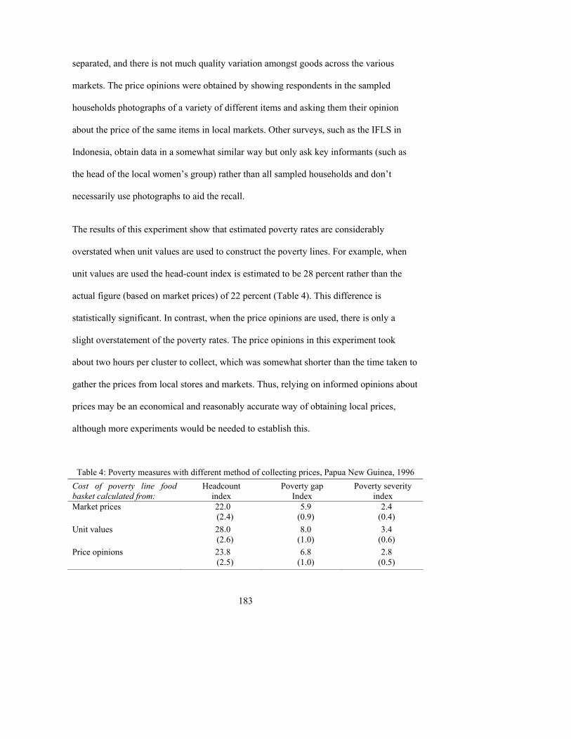
183
separated, and there is not much quality variation amongst goods across the various
markets. The price opinions were obtained by showing respondents in the sampled
households photographs of a variety of different items and asking them their opinion
about the price of the same items in local markets. Other surveys, such as the IFLS in
Indonesia, obtain data in a somewhat similar way but only ask key informants (such as
the head of the local women�s group) rather than all sampled households and don�t
necessarily use photographs to aid the recall.
The results of this experiment show that estimated poverty rates are considerably
overstated when unit values are used to construct the poverty lines. For example, when
unit values are used the head-count index is estimated to be 28 percent rather than the
actual figure (based on market prices) of 22 percent (Table 4). This difference is
statistically significant. In contrast, when the price opinions are used, there is only a
slight overstatement of the poverty rates. The price opinions in this experiment took
about two hours per cluster to collect, which was somewhat shorter than the time taken to
gather the prices from local stores and markets. Thus, relying on informed opinions about
prices may be an economical and reasonably accurate way of obtaining local prices,
although more experiments would be needed to establish this.
Table 4: Poverty measures with different method of collecting prices, Papua New Guinea, 1996 Cost of poverty line food basket calculated from:
Headcount index
Poverty gap Index
Poverty severity index
Market prices 22.0 (2.4)
5.9 (0.9)
2.4 (0.4)
Unit values 28.0 (2.6)
8.0 (1.0)
3.4 (0.6)
Price opinions 23.8 (2.5)
6.8 (1.0)
2.8 (0.5)
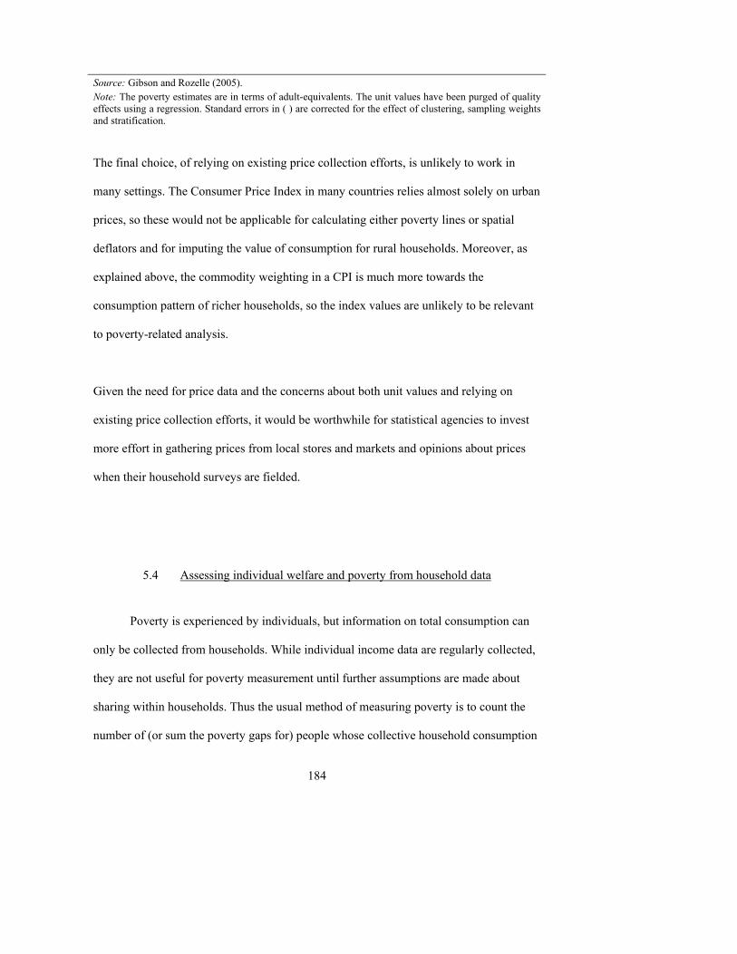
184
Source: Gibson and Rozelle (2005). Note: The poverty estimates are in terms of adult-equivalents. The unit values have been purged of quality effects using a regression. Standard errors in ( ) are corrected for the effect of clustering, sampling weights and stratification.
The final choice, of relying on existing price collection efforts, is unlikely to work in
many settings. The Consumer Price Index in many countries relies almost solely on urban
prices, so these would not be applicable for calculating either poverty lines or spatial
deflators and for imputing the value of consumption for rural households. Moreover, as
explained above, the commodity weighting in a CPI is much more towards the
consumption pattern of richer households, so the index values are unlikely to be relevant
to poverty-related analysis.
Given the need for price data and the concerns about both unit values and relying on
existing price collection efforts, it would be worthwhile for statistical agencies to invest
more effort in gathering prices from local stores and markets and opinions about prices
when their household surveys are fielded.
5.4 Assessing individual welfare and poverty from household data
Poverty is experienced by individuals, but information on total consumption can
only be collected from households. While individual income data are regularly collected,
they are not useful for poverty measurement until further assumptions are made about
sharing within households. Thus the usual method of measuring poverty is to count the
number of (or sum the poverty gaps for) people whose collective household consumption
185
expenditure (or income) is below the poverty line. Results may be presented on an
individual basis by weighting by household size. But the calculations are still
fundamentally household-based. The disconnect between the level at which data are
collected compared with the level at which analysis is desired raises two questions:
• Are there reliable methods of observing whether some types of individuals
within households, such as women or the elderly, are poorer than others in
the same household?
• How should adjustments be made for differences in household size and
composition when determing individual welfare and poverty status based
on household data?
The literature on intra-household inequality addresses the first issue. This
literature has yet to make much impact on the activities of statistical offices, partly
because of the practical difficulties involved. The second issue, which is addressed by the
literature on equivalence scales, is more widely recognised by statistical offices. Indeed,
approximately 30 of the countries providing metadata in the Statistical Addendum make
some allowance for equivalence scales when setting poverty lines and measuring poverty.
Because of this wider use by survey agencies, and also because equivalence scales have a
longer history, they are discussed first.
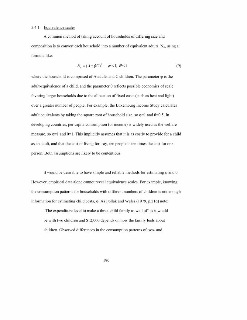
186
5.4.1 Equivalence scales
A common method of taking account of households of differing size and
composition is to convert each household into a number of equivalent adults, Ne, using a
formula like:
( ) 1, 1eN A C θϕ ϕ θ= + ≤ ≤ (9)
where the household is comprised of A adults and C children. The parameter φ is the
adult-equivalence of a child, and the parameter θ reflects possible economies of scale
favoring larger households due to the allocation of fixed costs (such as heat and light)
over a greater number of people. For example, the Luxemburg Income Study calculates
adult equivalents by taking the square root of household size, so φ=1 and θ=0.5. In
developing countries, per capita consumption (or income) is widely used as the welfare
measure, so φ=1 and θ=1. This implicitly assumes that it is as costly to provide for a child
as an adult, and that the cost of living for, say, ten people is ten times the cost for one
person. Both assumptions are likely to be contentious.
It would be desirable to have simple and reliable methods for estimating φ and θ.
However, empirical data alone cannot reveal equivalence scales. For example, knowing
the consumption patterns for households with different numbers of children is not enough
information for estimating child costs, φ. As Pollak and Wales (1979, p.216) note:
�The expenditure level to make a three-child family as well off as it would
be with two children and $12,000 depends on how the family feels about
children. Observed differences in the consumption patterns of two- and
187
three-child families cannot even tell us whether the third child is regarded
as a blessing or a curse.�
More formally, the problem is one of under-identification. It is possible to
construct two different cost functions that a household faces to reach a given utility level
and derive the same demand function from each one (Deaton, 1997). These different cost
functions can embody different attitudes of parents toward their children and different
elasticities of cost with respect to household size. Accordingly, observed demands do not
provide sufficient information to identify either the costs of children or their related
economies of scale.
Additional assumptions are needed to identify equivalence scales from observed
data on household consumption patterns. One approach is based on what is sometimes
called Engel�s second law, the assertion that the food share is an inverse indicator of
welfare across households of different sizes and compositions. There is no theoretical
justification for this Engel approach. Moreover, its empirical results are highly sensitive
to the measurement errors associated with certain data collection methods (Gibson,
2002). Thus, even though the approach is sketched below, it is not recommended.
Another approach is known as the Rothbarth method, where identification is
obtained from the assumption that adults' standard of living is indicated by the value of
expenditure on "adult goods" (goods not consumed by children). This approach can measure
the costs of children but not economies of scale. The equivalence scales from this method
188
are typically smaller than those calculated from the Engel method, which is known to
overstate the costs of children (Nicholson, 1976).
A third method compares the recommended daily allowances of nutrients, and
especially calories, for different age and gender groups to determine the adult equivalence of
a child. This assumes that relative food needs for children are the same as relative non-food
needs, which seems unlikely. Moreover, some controversy surrounds the definition and
use of nutrient requirements because it is not clear whether the lower requirements for,
say, women reflect lower needs or just the adaptation to receiving less by a historically
discriminated-against group (Sen, 1984).
Given these limitations, an appropriate goal for many statistical agencies may simply
be to use equation (9) to carry out sensitivity analyses, trying different values of φ and θ to
see whether any conclusions reached previously using per capita consumption are
overturned. This approach has highlighted, for example, that people in widow-headed
households in India are more likely than people in other households to be poor only if
economies of scale are important (Dreze and Srinivasan, 1997). Thus, conclusions about
gender and poverty may have to be conditioned on assumptions about economies of
scale.
An important detail when using equivalence scales, either for sensitivity analysis
or for the main poverty calculations, is that the scales should be applied symmetrically to
both the poverty line and the welfare indicator. This follows from the fact that the poverty
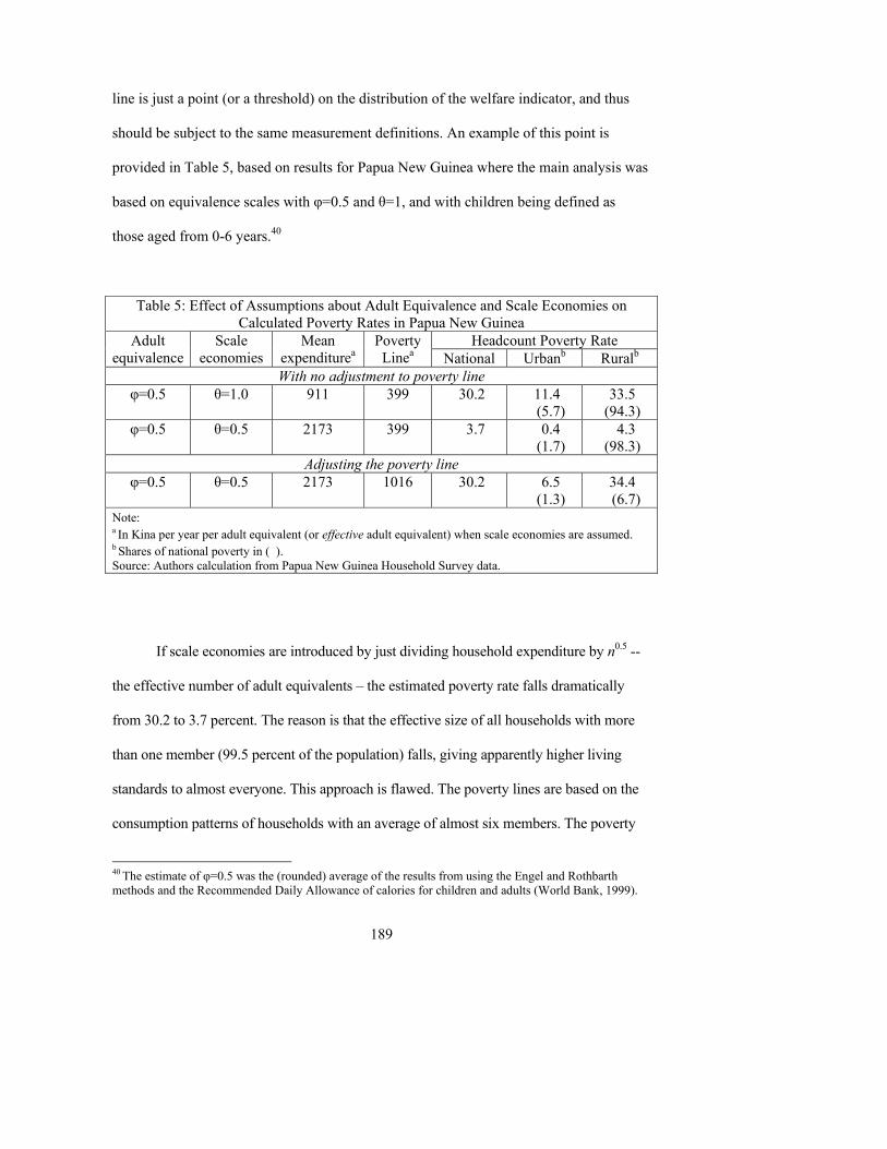
189
line is just a point (or a threshold) on the distribution of the welfare indicator, and thus
should be subject to the same measurement definitions. An example of this point is
provided in Table 5, based on results for Papua New Guinea where the main analysis was
based on equivalence scales with φ=0.5 and θ=1, and with children being defined as
those aged from 0-6 years.40
Table 5: Effect of Assumptions about Adult Equivalence and Scale Economies on Calculated Poverty Rates in Papua New Guinea
Headcount Poverty Rate Adult equivalence
Scale economies
Mean expenditurea
Poverty Linea National Urbanb Ruralb
With no adjustment to poverty line φ=0.5 θ=1.0 911 399 30.2 11.4
(5.7) 33.5
(94.3) φ=0.5 θ=0.5 2173 399 3.7 0.4
(1.7) 4.3
(98.3) Adjusting the poverty line
φ=0.5 θ=0.5 2173 1016 30.2 6.5 (1.3)
34.4 (6.7)
Note: a In Kina per year per adult equivalent (or effective adult equivalent) when scale economies are assumed. b Shares of national poverty in ( ). Source: Authors calculation from Papua New Guinea Household Survey data.
If scale economies are introduced by just dividing household expenditure by n0.5 --
the effective number of adult equivalents � the estimated poverty rate falls dramatically
from 30.2 to 3.7 percent. The reason is that the effective size of all households with more
than one member (99.5 percent of the population) falls, giving apparently higher living
standards to almost everyone. This approach is flawed. The poverty lines are based on the
consumption patterns of households with an average of almost six members. The poverty
40 The estimate of φ=0.5 was the (rounded) average of the results from using the Engel and Rothbarth methods and the Recommended Daily Allowance of calories for children and adults (World Bank, 1999).
190
lines would be higher if they were just based on single-person households because of the
diseconomies of living alone.
Ideally, all calculations used to derive the poverty line should rely on the same
equivalence scale applied to the welfare indicator. But in the absence of this
comprehensive approach, the poverty line may be adjusted in the following manner:
(i) find a household of average size and composition whose per capita
expenditure is equal to the poverty line, and
(ii) set the adjusted poverty line equal to whatever value their per-effective-
adult-equivalent expenditure becomes after the introduction of the
equivalence scale.
This rule ensures that a household of average size and composition remains above or
below the poverty line irrespective of the choice of equivalence scales (Dreze and and
Srinivasan, 1997). In the example in Table 5, this adjustment raises the poverty line from
K399 to K1016, and the national poverty rate returns to the previously calculated level of
30.2 percent.
Once a similar equivalence scale is applied to both the welfare indicator and the
poverty line, the main effect of assumptions about child costs and scale economies should
be to alter the poverty profile, rather than the aggregate poverty measurements. The
poverty profile for any characteristics associated with differences in household
composition and size, such as sector of residence, and the age and marital status of the
household head are likely to be sensitive to assumptions about equivalence scales. Thus,
191
in the example in Table 5, the introduction of scale economies reduces the share of
poverty in urban areas from 5.7 percent to 3.3 percent because urban households are
larger than rural households (7.0 versus 5.7 residents).
5.4.2 The Rothbarth method of measuring child costs
The Rothbarth method of measuring child costs starts, somewhat paradoxically, with
expenditures on goods that are not consumed by children--for example alcohol, gambling,
and tobacco. Expenditures on these goods should fall when children are added to the
household. Children bring additional consumption needs without any offsetting increase in
income so there is effectively less income available for the adults to spend on these �adult
goods�. Moreover, unlike other goods such as food, it is possible to rule out a direct demand
effect causing increased spending on these goods since child don�t gamble, smoke, and
drink alcohol. Therefore, the cost of a child can be measured by calculating the amount of
compensation that would have to be paid to parents to restore expenditure on adult goods to
the former level before the child was added to the family.
The Rothbarth method is illustrated in Figure 3, showing the relationship between
total household expenditure and expenditure on adult goods. Spending on adult goods rises
as total household expenditure increases, according to the schedule AB. For a reference
household composed of two adults, total expenditure is x0 and adult goods expenditure is
0 .Ax In comparison, a two-adult and one-child household spends less on adult goods at the
same level of total outlay because of the competing needs of the child. The household would
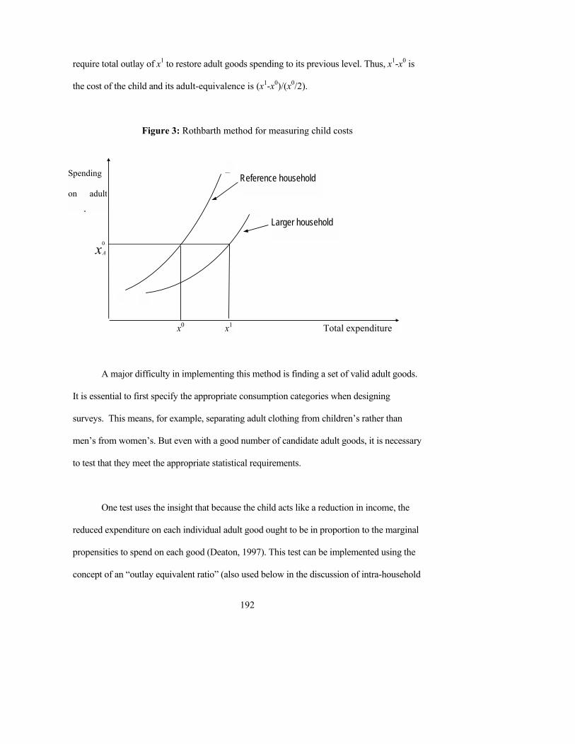
192
require total outlay of x1 to restore adult goods spending to its previous level. Thus, x1-x0 is
the cost of the child and its adult-equivalence is (x1-x0)/(x0/2).
Figure 3: Rothbarth method for measuring child costs
A major difficulty in implementing this method is finding a set of valid adult goods.
It is essential to first specify the appropriate consumption categories when designing
surveys. This means, for example, separating adult clothing from children�s rather than
men�s from women�s. But even with a good number of candidate adult goods, it is necessary
to test that they meet the appropriate statistical requirements.
One test uses the insight that because the child acts like a reduction in income, the
reduced expenditure on each individual adult good ought to be in proportion to the marginal
propensities to spend on each good (Deaton, 1997). This test can be implemented using the
concept of an �outlay equivalent ratio� (also used below in the discussion of intra-household
xA
0
x0 x1 Total expenditure
Reference household Spending
on adult
dLarger household
B
193
inequality), which can be obtained from an estimated regression of the budget share
equation for a good:
( ) ( )ln ln (10)J -1
i iii i ij ji i
j=1
p q = = + x n + n + n n +w ux β η γα ∑
where the product (of price and quantity) piqi is the expenditure on good i, wi is its budget
share, x is the value of total household consumption expenditure, n is total household size, nj
is the number of people in the jth demographic group, and ui is a residual. Coefficients from
equation (10) can be used to calculate outlay equivalent ratios for each good:
( )(11)
J
jiji i irj=1
ir
ii
( - ) + - nn =
+ w
η β γ γπ
β
∑
(sample means can be used for the wi and the nj /n ratios). The ratio, πir measures the effect
of an additional person of type r on the demand for good i in terms of the percentage change
in outlay (expenditure) per person that would have been necessary to produce the same
effect on demand. For any particular type of child group (say, 0-6 year-old boys) the outlay
equivalent ratios should be the same across a set of valid adult goods (subject to sampling
variability).
Once a set of adult goods have been identified, equation (10) can be used to find the
budget share and expenditure on an adult good for a reference household. In principle, this
can be calculated with a single adult good. But improved statistical precision may occur if
all of the valid adult goods are aggregated into a combined category. The equation is then
used to recalculate the adult goods expenditure after a child is added to the reference
household. The final step is to calculate how much household total expenditure would have
194
to increase to restore adult goods expenditure to its initial level. For example, a poverty
assessment in Papua New Guinea used this approach and found that adding an older child
(7-14 years of age) to a 2-adult household would require a 31 percent increase in total
expenditures to restore adult goods expenditure to their previous level (World Bank, 1999).
Thus, the adult-equivalence of an older child was approximately 0.6 of an adult.
5.4.3 The Engel method of measuring child costs
Figure 4 shows how the Engel method works. The food share is plotted against
total household expenditure for a reference household with two adults and for a
household that also has a child. At any given level of total expenditures, for example x0,
the household with children has a larger food share than does the reference household.
Assuming that the food share is an inverse welfare measure across household types,
individuals in the household with children appear worse off. The household with children
would need total expenditures of x1 to have the same food budget share, and thus the
same welfare level as the reference household. Therefore, x1-x0 is a measure of child costs
and the adult-equivalence of a child is (x1-x0)/(x0/2). This can be worked out from the
parameters of a food Engel curve like equation (10).
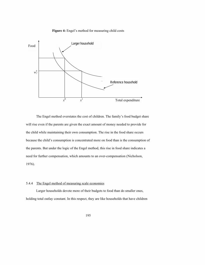
195
Figure 4: Engel�s method for measuring child costs
The Engel method overstates the cost of children. The family�s food budget share
will rise even if the parents are given the exact amount of money needed to provide for
the child while maintaining their own consumption. The rise in the food share occurs
because the child�s consumption is concentrated more on food than is the consumption of
the parents. But under the logic of the Engel method, this rise in food share indicates a
need for further compensation, which amounts to an over-compensation (Nicholson,
1976).
5.4.4 The Engel method of measuring scale economies
Larger households devote more of their budgets to food than do smaller ones,
holding total outlay constant. In this respect, they are like households that have children
w f0
x0 x1 Total expenditure
Reference household
Food Larger household
B
196
(whose consumption is concentrated more on food than is the consumption by adults), so
the Engel method of measuring child costs is readily adapted to the measurement of scale
economies. For example, the approach illustrated in Figure 4 could be extended by
plotting a family of Engel curves and calculating the extra expenditure (xk-x0) needed for
households of size n0+k (where k=1,2,3,�).
The regression approach in equation (10) can also be adapted, using nθ instead of
n as the measure of household size. Thus, if x0 is the outlay of a one-person household, an
n-person household of the same composition needs a total outlay of x0nθ to have the same
food share (and the same welfare level, by assumption). For example, Lanjouw and
Ravallion (1995) estimate θ to be 0.6 in Pakistan, so if 10 individuals formed a 10-person
household, their per-capita food spending could decline by 60 percent and according to
the Engel method they would still have the same level of welfare (100.6=3.98). These
large estimates of scale economies have attracted some criticism because they imply
improbably large reductions in food spending by consumers in a poor country with
considerable under-nutrition (Deaton, 1997).
Unfortunately, the Engel method makes no more sense for measuring scale
economies than it does for measuring child costs. Consider a larger household with the
same per capita expenditures as a smaller household. If there are scale economies, the
larger household is better off. Thus, according to Engel�s second law, the larger
household should have a lower food share. But a decline in the food share with constant
per capita expenditures can occur only if there is a decline in food spending per person. It
197
is very unlikely that people who are better off would spend less on food, especially in
poor countries where nutritional needs are not being met.
In addition to this conceptual problem, the Engel method does not give robust
empirical estimates of scale economies. In an experiment in Port Moresby, the capital
city of Papua New Guinea, the Engel estimate of θ was 0.76 (and not statistically
significantly different from 1.0, implying no scale economies) for a half sample whose
expenditures were surveyed with diaries. However, in the other half-sample, where a
recall survey was used, the Engel estimate of θ was 0.41, implying large economies of
scale (Gibson, 2002). This evidence is problematic because estimates of scale economies
should not depend on the method used to gather expenditure data. The conceptual and
empirical problems with the Engel method suggest that it is a statistical tool that should
not be used for poverty measurement.
5.4.5 Adjusting poverty statistics when adult equivalents are units
Poverty gap measures may need modifying when the welfare indicator and
poverty line are measured in adult equivalent rather than per capita terms. The standard
FGT formula uses the number of people, N, and the number of poor people,
Q: ( )11
1 ( ) .Q
ii
P z y zN =
= −∑ The monetary poverty gap can be calculated as: 1P N z× × , but
this will exaggerate the cost of closing the gap when adult equivalents are used.
For example, consider a two-adult and two-child household with total annual
expenditure of $1,200. The poverty line is set at $500 per adult equivalent, and children
198
count as 0.5 adults. Comparing expenditure per adult equivalent ($400) with the poverty
line indicates an average gap of $100 and a P1 measure of 0.2. If P1 is multiplied by
N z× , the aggregate value of the poverty gap will appear to be $400. But in fact it is only
$300. One way to prevent this overstatement is to estimate all poverty measures using
adult equivalent numbers rather than person numbers, even though these may not be the
most familiar units for communicating the results. An alternative is to use correction
formulae suggested by Milanovic (2002).
5.4.6 Methods for estimating the intra-household allocation of consumption
Several procedures have been suggested for using household data to see if some
types of individuals are poorer than others within the same household. There has been
limited success with these procedures, and it is likely to be several years before statistical
offices would consider routinely applying them. Nevertheless, greater awareness of these
procedures may be helpful, especially if it leads to the collection of data that are better
suited to the needs of these methods.
In the Rothbarth method of measuring child costs discussed above, children exert
negative income effects on the demand for adult goods. If some types of children have
larger income effects than others, it may provide evidence of a gender bias within the
household. For example, if outlay equivalent ratios (see equation (11)) are more negative
for boys than for girls, this suggests that parents cut back their own consumption more
when a boy is added to the household than when a girl is added (Deaton, 1989).
199
Unfortunately, most applications of the adult goods method have produced
puzzling results, sometimes finding bias against girls in locations where it is not expected
and no bias in places where other evidence strongly suggests that boys are favoured
(Deaton, 1997). It is possible that part of this failure reflects the coarseness of the data
collected in many household surveys, which have rather few adult goods disaggregated. In
one of the few applications where the method worked as expected, the questionnaire had
contained a set of well-defined categories for adult goods because the test for gender bias
had been planned when the data were collected (Gibson and Rozelle, 2004).
It is harder to study unequal allocations between adults because differences in
demand � even if observed at an individual level � may just reflect differences in
preferences. These differences in preferences can be ignored when the adult-goods
method is applied to children who exert only income effects (because they don�t consume
the goods themselves). Some headway in identifying �sharing rules� for the allocation of
consumption between adults in the same household has been made by Bourguignon and
Chiappori (1992). They identify the sharing rule using either �assignable goods� or
�exclusive goods�. An assignable good is a private good (that is, a good where the
consumption by one person subtracts from the consumption of another) whose
consumption by each member of the household can be observed. An exclusive good is a
private good used by only one member of the household. Progress in applying these
methods may be aided by household surveys that use diaries for each adult, rather than
household level reporting, and that also collect information on whether purchases are
200
destined to be consumed by the purchaser (the diary-keeper) or someone else (Browning
et al, 2003).
5.4.7 Collecting non-monetary data on individuals to estimate gender-specific measures of poverty Most household surveys collect information on non-monetary welfare indicators
such as education and, less frequently, health. These data are usually collected for each
individual in the household and offer the possibility of assessing individual poverty, at
least in a non-monetary sense. Comparisons of educational attainment and participation
for women relative to men are regularly made with such data. Comparisons of health
status can also be made, especially using anthropometric data. It has also been claimed by
Case and Deaton (2002) that self-reported data on health can prove useful.
In these surveys of self-reported health, respondents are asked to rate their overall
health status on a 5-point scale, ranging from �excellent� to �poor.� There can be a
considerable amount of adaptation to poor living conditions, which hampers comparisons
of self-rated health across communities and countries. But within individual
communities, comparisons are not affected by this adaptation, and these comparisons
suggest that women�s self-rated health is worse than men�s (Case and Deaton, 2002). At
least in the short-run, there may be more success at understanding the gender dimensions
of poverty using broader health and education measures than there is from attempting to
untangle consumption of individuals within the household.
201
5.5 Conclusion
This chapter described some of the methods and data available for measuring
poverty with cross-sectional household surveys. These surveys are the workhorse of
poverty analysis, in part because all countries have at least one cross-sectional household
survey of one type or other. Many of these surveys were not originally designed with
poverty measurement as a key aim and have certain features, such as short reference
periods and limited topical coverage, that limit their usefulness as a source of data for
understanding poverty. However, some modest modifications of survey practice that are
suggested in this chapter could improve the quality of poverty measurements coming
from these surveys.
Another theme of the chapter is the need for consistent survey methods so that
poverty comparisons uncover real changes in the population rather than artifacts that are
due to variation in survey design. Examples from India and Cambodia show how large
the effects seemingly minor variations in survey design can have on poverty estimates. It
would be a welcome addition to current practice if all statistical agencies carried out
detailed experiments to assess the effect on measured poverty rates when they change
survey methods, so that adjustment factors can be calculated and robust poverty trends
retrieved.
Sensitivity of poverty estimates to variations in survey design also highlights the
importance of measurement error. A previous emphasis on means and totals as the
202
statistics of interest may have lulled some survey agencies into a belief that random
measurement errors do not matter so long as they cancel out. However this is not true in
the context of poverty and inequality measurement. Accordingly, statistical agencies
should increase the efforts made to improve the accuracy of their household survey data.
203
References Bourguignon, F. and Chiappori, P.-A. (1992). Collective models of household behaviour: an introduction.
European Economic Review, 36, 355-364.
Browning, M., Bonke, J., and Uldall-Poulsen, H. (2003). The intra-household allocation of expenditures: new survey evidence from Denmark. The 2003 IAREP Workshop on Household Economic Decisions: Earning, Sharing, Spending and Investing Money, 5-7 December, Agder University College, Kristiansand, Norway.
Capéau, B. and Dercon, S. (1998). Prices, Local Measurement Units and Subsistence Consumption in Rural Surveys : An Econometric Approach with an Application to Ethiopia. (Working Paper 98-10). Oxford : Oxford University, Centre for the Study of African Economies.
Case, A. and Deaton, A. (2002). Consumption, Health, Gender and Poverty. (Mimeo). Princeton, NJ : Princeton University, Research Program in Development Studies.
Central Statistical Office (1995). Republic of Zambia Household Budget Survey, 1993-94, Volume 1 � Main Tables and Report Lusaka.
Deaton, A. (1989). Looking for boy-girl discrimination in household expenditure data. World Bank Economic Review, 3(1): 1-15.
Deaton, A. (1997). The Analysis of Household Surveys: A Microeconometric Approach to Development Policy. Baltimore : Johns Hopkins University Press.
Deaton, A. (2001). Counting the world�s poor: Problems and possible solutions. World Bank Research Observer, 16(2), 125-147.
Deaton, A. (2003). Prices and poverty in India: 1987-2000. Economic and Political Weekly, Jan 25, 362-368.
Deaton, A. (2005). Measuring poverty in a growing world (or measuring growth in a poor world). Review
of Economics and Statistics, 87(1): 1-19.
Deaton, A. and Grosh, M. (2000). Consumption. In Grosh, M. and Glewwe, P. (eds) Designing Household Survey Questionnaires for Developing Countries (pp. 91-133). Washington, D.C. : The World Bank.
Deaton, A. and Zaidi, S. (2002). Guidelines for Constructing Consumption Aggregates for Welfare Analysis. (Living Standards Measurement Study, working paper no. 135). Washington, D.C. : The World Bank.
Dreze, J., and Srinivasan, P. V. (1997). Widowhood and poverty in rural India: some inferences from household survey data. Journal of Development Economics, 54(2), 217-234.
Filmer, D., and Pritchett, L. H. (2001). Estimating wealth effects without expenditure data - or tears: An application to educational enrollments in states of India. Demography, 38(1), 115-132.
Gibson, J. (1999). Can women�s education aid economic development? The effect on child stunting in
Papua New Guinea. Pacific Economic Bulletin, 14(2): 71-81.
Gibson, J. (2000). A Poverty Profile of Cambodia, 1999. A Report to the World Bank and the Ministry of Planning, Phnom Penh, Cambodia.
Gibson, J. (2001). Measuring chronic poverty without a panel. Journal of Development Economics, 65(2), 243-266.
Gibson, J. (2002). Why does the Engel method work? Food demand, economies of size and household survey methods. Oxford Bulletin of Economics and Statistics, 64(4), 341-360.
204
Gibson, J., Huang, J. and Rozelle, S. (2003). Improving estimates of inequality and poverty from urban China�s Household Income and Expenditure survey. Review of Income and Wealth, 49(1), 53-68.
Gibson, J. and Rozelle, S. (2004). Is it better to be a boy? A disaggregated outlay-equivalent analysis of gender bias in Papua New Guinea. Journal of Development Studies, 40(4): 115-136.
Gibson, J. and Rozelle, S. (2005). Prices and unit values in poverty measurement and tax reform analysis. World Bank Economic Review, 19(1): 69-97.
Grosh, M. and Glewwe, P. (2000). Designing Household Survey Questionnaires for Developing Countries, Washington, D.C. : The World Bank.
Howes, S. and Lanjouw, J. (1998). Does sample design matter for poverty rate comparisons. Review of Income and Wealth, 44(1), 99-110.
Jolliffe, D. (2001). Measuring absolute and relative poverty: the sensitivity of estimated household consumption to survey design. Journal of Economic and Social Measurement, 27(1), 1-23.
Jorgenson, D. (1998). Did we lose the war on poverty? Journal of Economic Perspectives, 12(1), 79-96.
Korn, E. and Graubard, B. (1999). Analysis of Health Surveys New York: John Wiley and Sons.
Lanjouw, J. and Lanjouw, P. (2001). How to compare apples and oranges: Poverty measurement based on different definitions of consumption. Review of Income and Wealth, 47(1), 25-42.
Lanjouw, P. and Ravallion, M. (1995). Poverty and household size. The Economic Journal, 105 (433), 1415-1434.
Milanovic, B. (1979). Do we tend to overestimate poverty gaps? The impact of equivalency scales on the calculation of the poverty gap. Applied Economics Letters, 9(1), 69-72.
Mukherjee, S. (2005) On asset indices. Mimeo Department of Economics, Princeton University.
Neter, J. and Waksburg, J. (1964). A study of response errors in expenditure data from household interviews. Journal of the American Statistical Association, 59(305): 18-55.
Nicholson, J. L. (1976). Appraisal of different methods of estimating equivalence scales and their results. Review of Income and Wealth, 22(1), 1-11.
Pollak, R. A., and Wales, T. J. (1979). Welfare comparisons and equivalence scales. American Economic Review, 69(2), 216-221.
Pradhan, M. (2001). Welfare Analysis with a Proxy Consumption Measure: Evidence from a Repeated Experiment in Indonesia. (Mimeo) Amsterdam : Free University.
Pradhan, M., Suryahadi, A., Sumarto, S., and Pritchett, L. (2001). Eating like which �Joneses?� An iterative solution to the choice of a poverty line reference group. Review of Income and Wealth 47(4): 473-487.
Prais, S. (1958). Whose cost of living? Review of Economic Studies 26(1): 126-134.
Ravallion, M. (1994). Poverty Comparisons. Chur : Harwood Academic Publishers.
Ravallion, M. (2003). Measuring aggregate welfare in developing countries: how well do national accounts and surveys agree? Review of Economics and Statistics, 85(3): 645-652.
Sahn, D. E., and Stifel, D. (2000). Poverty comparisons over time and across countries in Africa. World Development, 28(12), 2123-2155.
Scott, C. (1992). Estimation of annual expenditure from one-month cross-sectional data in a household
survey. Inter-Stat, 8, 57-65.
Scott, C. and Amenuvegbe, B. (1991). Recall loss and recall duration: an experimental study in Ghana. Inter-Stat, 4(1), 31-55.
205
Scott, K., and Okrasa, W. (1998). Analysis of Latvia Diary Experiment. Washington, D.C. : World Bank, Development Research Group.
Sen, A.K. (1984). Family and food: sex bias in poverty. in Resources, Values and Development, Oxford University Press, Delhi.
Slesnick, D. (1993). Gaining ground: poverty in the postwar United States. Journal of Political Economy. 101(1), 1-38.
Tarozzi, A. (2004). Calculating comparable statistics from incomparable surveys, with an application to poverty in India. Paper presented at the North East Universities Development Consortium Conference, Montreal, October 2004, available at http://www.hec.ca/neudc2004/Programme2.html
UNICEF, (1998). State of the World�s Children Report, Oxford University Press: New York.
U.S. Census Bureau. (2003). CENVAR [Software]. http://www.census.gov/ipc/www/imps/cv.htm
World Bank. (1999). Papua New Guinea: Poverty and Access to Public Services Washington, DC: World Bank.
206
CHAPTER VI. STATISTICAL ISSUES IN MEASURING POVERTY FROM NON-HOUSEHOLD SURVEYS SOURCES
Gisele Kamanou, Michael Ward and Ivo Havinga
Introduction
This chapter provides an overview of the wide range of non-household survey and
administrative data sources often on hand to amplify a broader understanding of poverty
and the poor. This information can help describe the social context and type of society
that preserves such conditions among low-income households. It highlights the multi-
dimensional nature of poverty and the different situations people encounter as they try to
escape poverty. The discussion explores the possibility of supplementing the deductive
analysis permitted by a scientifically-designed household sample survey, where
conditions observed are formally extrapolated to a predefined universe, to provide a
greater understanding of the population under investigation. Such household survey
information can then be complemented with related official indicators and less
conventional data drawn from less rigorous and formal inductive survey procedures.
Household-based surveys, both cross-sectional and longitudinal, provide
important economic and social information about the human condition. Cross-sectional
207
surveys tend to inform on the nature and status of individuals and the households they
belong to. Longitudinal surveys reveal how people are affected by, and adjust to,
changing circumstances over time. But such surveys are imperfect instruments of inquiry
because they suffer from varying and often indeterminate item expenditure non-response
as well as household unit non-response. The data collected in household surveys are also
subject to observation and measurement errors. Most importantly, they sometimes fail to
pick up key information at the extremes of spending lifestyles because their scope misses
out certain consumption behaviour of very poor and very rich households. Data compiled
from conventional household surveys thus need to be supplemented by information
collected about individuals from additional and, in some cases, with more comprehensive
and extensive coverage but less detailed questions.
Researchers are willing to relinquish some of the benefits of a standard survey
(based on recognized probability sampling methods that generate known means and
standard errors of the estimates) because they can trade them off against a more
qualitative approach that tries to touch on relationships and identify the purposes behind
individual activities. Adoption of qualitative survey methods offers the opportunity for
more penetrating insight into how certain groups of people behave and respond to
different socioeconomic stimuli and policy initiatives. With inductive approaches of this
nature, the primary problem is to identify the appropriate universe to which the observed
characteristics of the selected sample apply. The procedure recognizes the advantages of
advancing non-scientific methods to reduce the non-sampling errors (at the expense of
208
introducing an unknown sampling error) and to amplify the underlying picture and
provide greater in-depth knowledge about a given situation.
6.1 Prospects for expanding the poverty Database
Apart from improving household survey methodology and significantly extending
data coverage, the primary means of expanding the Database is to amplify and strengthen
survey findings with routine administrative data collection procedures and to bring in
alternative survey sources. Expanding already complex multi-topic household surveys is
proving to be increasingly expensive, and extending these surveys involves, in many
instances, implementation of an even wider multi-facetted approach.
Administrative information is required to provide a comprehensive perspective
and to give specified contextual population relevance to the more detailed survey
findings. Combining administrative records and survey sources can throw clearer light on
a problem and its multiple dimensions. Introduction of official data from regular reports
provides analysts with the ability to monitor more consistently what is transpiring on an
annual basis. In the case of poverty analysis, this may be especially relevant if the
characteristics of the poorest households, such as their size, age and sex composition, as
well as the nature of their habitation and where they live and, indeed, how they use this
209
asset, is markedly different from the majority of households covered in a traditional
survey.
It is increasingly accepted, though not yet common, to supplement the results
from national household surveys with other useful information, mostly of an official
nature, that is currently available �off-the peg� from existing files and documents and
from special searches of other sources. Administrative files provide a first line of
potentially useful information in this connection, especially in those instances where
attention is paid by policy-makers to disadvantaged groups and where officials are
required to monitor conditions and report on actions taken in this area. Importantly, from
a statistical perspective, the sample for a general household survey will usually have been
designed with objectives that do not focus specifically on obtaining, in an optimal way,
key information about the poorest households in the community. Most surveys of this
nature would require a higher sampling fraction for poor households [or, more precisely,
of the areas in which such households are most likely to be found]. And this would have
to be greater the lower the expected level of incidence or frequency of poor households.
All this raises costs because it is rarely possible to lower the sampling fraction for the rest
of the survey to compensate for the need to sample poor households more intensively.
If compromises are not made, like reducing topic coverage, then it is quite
possible the authorities may decide to conduct such large-scale surveys less frequently
and to rely increasingly on other sources of information. The same governments,
210
however, will probably continue to demand annual updates of key national and, possibly,
urban-rural data. They may also demand data on a more politically sensitive regional
basis. For this, more comprehensive national data series, such as the national accounts
and related indicators, will be required.
6.2 Limitations of Household Surveys for Poverty Assessment
Intangible institutional factors and cultural influences underline some of the
difficulties that limit complete reliance on conventional household survey data to
understand the extent and nature of poverty. Such surveys are also expensive and difficult
to manage. They cannot be conducted every year in most developing countries, especially
without substantial and continued outside support, and the continuity of monitoring is
often lost.
Some observers have also questioned whether the unitary household, as initially
defined by the census, and thus applied in all associated surveys, is entirely appropriate
for all kinds of poverty research. For some purposes, the extended family may be more
relevant, particularly when interpreting the production, consumption, and social
protection activities of nuclear units and how each functions. Understanding the nature of
the unit is important to understand intra-household transfers and different sharing
mechanisms. In other circumstances, it is the individual who should be the main focus of
211
attention. In the OECD, for example, there is considerable policy concern about child
poverty. Low-wage employment and the relationship of household well-being to the
unemployment or disability, whether permanent or transitory, of the head of the
household are equally important social policy concerns.
An important limitation of the standard approach in connection with poverty
inquiries is that a survey is not a very refined instrument for analyzing regional variations
within households. If, with given resources and an expected error acceptance/tolerance
level, the size of the survey has been predetermined and optimally designed to serve
some more general purpose, and if the number of households thought to be poor
represents, say, 20 percent of the total population, then the survey will not generate
meaningful estimates of poverty characteristics. Nor will it provide, detailed,
representative data covering different areas of inquiry and locations.
As indicated above, a significant limitation of the standard household survey is
that it usually provides only a single (albeit important) snapshot of poverty as it pertains
to a well-defined survey period. Policy analysts, however, are more interested in how
poverty changes over time, particularly in response to various policy initiatives and the
general increase (or decrease) in household incomes. Tracking changes implies a
dependence on more regular reporting methods that arise as a by-product of routine
administrative processes. The problem is then one of choosing the most relevant official
indicators as proxies for changes in the substantive variable under investigation.
212
Some researchers have suggested use of a master sample with a defined frame
that permits a number of related inquiries to be undertaken simultaneously or sequentially
addresses the issue of multi-dimensionality. It would allow large surveys to be
supplemented between years by much smaller surveys that are more specifically focused
on poverty issues. While this is an alternative way of circumventing the difficulty of
handling the above issues, the approach retains the overall integrity of the survey
methodology and master sample framework, preserving the inherent consistency and
comparability of the estimates. But it also poses its own set of problems. In particular, it
is complex from an organizational standpoint, and it tends to ignore the practical
difficulties of maintaining a comprehensive listing and of correctly and efficiently
updating the required frame on a regular basis to achieve the desired level of coherence
and sequential consistency.
From an international policy perspective, it is clearly desirable to have
comparable data on poverty across countries to obtain a common overview of the
problem and its characteristics. Although there are standard survey methods for
computing difficult values like imputed income from self-production and income from
home ownership, the absence, in practice, of a common international treatment of these
issues and of a harmonized questionnaire and associated data collection procedures,
hampers comparability. From a procedural standpoint, the pattern of non-response from
213
responding households and their specific response ranges/levels on different issues varies
between countries.
6.3 Integrating Different Data Techniques and Sources
For the above technical and practical reasons, delving into other official sources
that concentrate on the conditions and status of individuals [instead of the households to
which they belong] and bringing in other �topic specific� survey approaches is clearly
important.
Closer integration of quantitative and qualitative approaches through the selective
combination of survey methods and administrative data sources is intended to provide a
better and more comprehensive perspective on the scope of poverty. While no specific
course of action is advocated, the potential of matching in-depth analysis and results
offered by small well-focused samples and mapping the findings on to larger
scientifically designed surveys and benchmark reference databases together offer one of
the more promising ways to strengthen existing knowledge. Information gathered to
enhance the policy-makers� understanding of the varied and wide ranging issues involved
in tackling poverty should allow them to refine the analysis and to place the required
emphasis of action on specific regions and target groups at risk.
Adoption of mixed-method techniques usually means having to resort to different
institutional sources and quite independent non-official inquiry methods. It implies a
214
reliance on a wide variety of perhaps questionable data sources when bringing relevant
information to bear on the poverty problem. Because they observe different mandates
and have other defined objectives, many organizations may not focus primarily on
poverty. Furthermore, because of the difficulties of balancing the conflicting demands of
sample size, survey costs, and information requirements--and because they are not
basically statistical agencies--some sources do not compile quality data. Nevertheless,
provided care is taken to identify potential biases, researchers should not pass up the
opportunity of making selective use of any readily available related information that
cannot be gleaned from official sources.
Household survey results tend to be generated at rather infrequent [and usually
irregular] intervals, whereas much of the administrative data on official files is reported
annually and (like wages and prices) may be compiled at more frequent intervals. An
important part of the survey story will relate to the non-market activities of the household
sector. These activities are invariably less easy to quantify at the individual and
household �use� level and need to be complemented with official data on facilities,
service supply, and effective delivery.
Ability to draw together the micro and macro factors that impact poverty and to
blend the material and non-material elements that comprise the market and non-market
aspects of household behavior forms the basis of a more holistic perspective of the
poverty problem. A comprehensive database can yield insights into intangible issues,
215
such as differential access of households at different income levels to the opportunities,
entitlements, and various forms of official service support open to the public.
The logical starting point is to review the miscellaneous kinds of information
resources already available and make an assessment of how they can be used to give
greater depth and background to the core household survey information. Practical
experience in the use of such material will offer hints and suggest guidelines about how
existing reporting procedures can be modified to make them more relevant and reliable.
The main non-survey (administrative) sources and non-household survey methods that
may be employed to broaden the approach and their limitations are described in more
detail in the sections below.
In addition to the more variegated picture related data sources lend to any status
evaluation, establishment of acknowledged benchmarks linked to the decennial census
[and to any embedded sample census module], or that can be supported in the interim by
data from a quinquennial partial census, enable analysts to obtain a reasonable idea about
overall trends in poverty related to social and demographic change.
6.4 Multi-dimensional Nature of Poverty
216
Universal political consensus was achieved in 2000 on the core Millennium
Development Goals [MDGs], together with the joint agreement between countries on a
set of standard indicators and targets. These indicators were correspondingly established
to assess progress towards the accomplishment of the eight major articles of international
development policy. And there was national agreement to monitor them regularly. This
consensus has given common direction to poverty inquiries, and greater global
recognition to the diverse and multi-dimensional nature of poverty. The higher political
profile given to poverty eradication has concentrated popular attention on relative
deprivation and its possible causes. The MDGs underline the importance of looking more
comprehensively at the combination of both material and non-material goods and
services available for use by households to raise their general living standards. These
commodities originate from market and non-market sources, and their consumption
represents both the outcome of sovereign choice and the government�s own contribution
to well-being by supplying public goods and services designed to satisfy both individual
and collective needs. In the developing world, this crucial provision of �free� non-market
goods and services that are clearly valued and used by households, is also undertaken by
NGOs. The MDGs have helped direct public attention to the imbalances between various
sections of the population with respect to the disparities in lifestyles they experience,
their comparative ease of access to public facilities, and their ability to gain a ready
command over the range of public goods and services potentially available to them.
This section thus explores what respective data sources, beyond those of
household surveys with an alleged national coverage and those utilized in the broadly
217
based national accounts, should be sought to help expand knowledge about poverty--its
incidence, severity, and extent. Relevance and reliability of additional data sources and
their limitations, and the techniques adopted to exploit them, are discussed below. This
appeal to the broader concept of data mining reflects a rapidly developing interest in this
area of statistical analysis. It acknowledges that it is generally cheaper to review and take
what is already available than to launch an entirely new survey, ab initio. However,
changes in these formal sources may be similarly taking place as governments redefine
administrative directives and departmental responsibilities in line with new policy
objectives.
Detailed analysis of public sector accounts supplied by government for direct use
by the population that identifies expenditures on goods and services � though it does not
effectively assess how fairly these are delivered to intended recipients - is a prerequisite
for understanding what the government spends and how well it has been able to respond
to the needs of the people. The pattern and allocation of official spending may not
necessarily correspond to the officially perceived needs of people. Given the existing
scope of inequality, the ability of any government to carry out a poverty reduction policy,
especially strategies that combine conventional economic growth and marginal income
redistribution through taxation, can only be tested by seeing how far the extra resources
generated in the economy are spent on improving those health and educational services
available to the poorest households and regions.
218
The MDGs and their associated targets are shown in the annex of this Handbook.
This listing begins the process of identifying and distinguishing between,
• those parts of the compact that are susceptible to direct action by the
resident agencies with direct responsibility for such issues, and,
• those that depend on the national government to implement
appropriate pro-poor macroeconomic policy or on international action
that brings benefits.
6.5 Poverty Measures and the Millennium Development Goals
There are only two poverty measures that are directly defined in the MDGs. One
is concerned with the scope of poverty (total number of poor people), the other focuses
on the extent and severity of poverty. The depth of poverty reflects the degree to which
poor people�s incomes fall short, on average, of an officially recognized minimum
threshold level. Even this measure does not identify all those households and families that
societies normally regard as �living in the depths of poverty� or �on the edge of
existence.� So other classifications may be needed to distinguish, �the poorest of the
poor.� Traditionally, certain single measures--such as the extent of malnutrition or degree
of unemployment among unskilled workers--have been regarded as key indicators of
poverty. Selected indicators used to determine which groups go hungry are seen by many
as defining whether someone can be regarded as poor or not.
219
6.5.1 Relevance of the MDGs
By drawing attention to the general aspects of deprivation, MDGs have
underscored the wider multi-dimensional and inter-connected nature of poverty. Even
the most casual empirical analysis cannot fail to notice that malnutrition, inadequate
shelter, unsanitary living conditions, lack of clean water, poor solid waste disposal, low
educational achievement combined with the absence of proper schooling, chronic ill
health and widespread crime are salient features of poverty. Each of these facets needs to
be quantified to determine the degree of poverty and assess the strength of poverty�s
inter-relationships with other characteristics that appear to sustain it.
A key problem is that independent statistical information on such matters--where
it exists--is generally available only at the national level mostly from official
administrative sources. To enhance their relevance, national data also need to be
disaggregated by socio-economic category or, at the very least, by distinct locations small
enough to assist in the identification of those belonging to constituent population groups.
This will make it easier to see the problems poor people face and help investigate their
specific levels of existence and patterns of living and thus help policy initiatives target
needs.
220
Small area sampling procedures that can help examine these issues pose a
complex range of technical, methodological, and practical questions, especially in
relation to the frame and universe to which the studies refer. For the most part, smaller
and specifically targeted socio-economic surveys are rarely conducted directly by
national statistical offices [although some official studies may be outsourced]. This
makes it difficult to fully integrate a small sample survey�s results into an established
national benchmark.
6.5.2 Significance of non-market goods and services
It is desirable to compile data not only about material living standards (where
these can be seen primarily as the outcome of consumption preferences as revealed by the
actual choices people make in the market), but also about how non-material goods and
services are distributed among households. In the absence of suitable available files, such
details have to be picked up from a variety of public and private sources of information.
Compilation of indirect and partial data, collected mostly to serve miscellaneous
bureaucratic purposes and record administrative actions and decisions, is important for
building a more comprehensive picture of people�s living conditions.
This information extends beyond simple calibration of an individual household�s
sovereignty over the market supply of consumption goods and services; it touches on the
total supply of commodities on which value is placed by the community. To this should
be added, in any overall assessment of poverty, data about the value of social benefits to
221
which some households may be entitled and on social transfers they receive voluntarily
on a fairly regular basis.
6.6 Problem of determining Causes and Effects
Are the identifiable features of poor living conditions and social deprivation the
causes or effects of persistent poverty--or both? In the past, it was common for
politicians to refer to �the vicious circle of poverty� because it was difficult to
disentangle the endogenous from exogenous factors affecting the condition and thus to
distinguish the initial cause and effect. But, it is widely assumed that general economic
and fiscal policy [i.e., tax, subsidy and transfer actions as well as ministerial spending
decisions] can together play a crucial role in this equation. A coherent fiscal strategy may
be more relevant and probably more sustainable than a difficult-to-define �pro-poor�
growth policy. In other words, if it is the government�s intent to conduct a fair and
equitable social policy that will pay special attention to the needs of the poor over the
longer term, then it may not be necessary to distort the core thrust of economic policy and
upset the basic quest for overall real income growth.
But, by the same token, government must maintain consistent oversight of where
the progressive incidence of its taxes fall and monitor the socio-economic distribution of
government expenditures destined for collective and individual household consumption.
222
This requires national statistical offices to prepare, in the interests of distributive social
justice, beneficiary accounts that detail the allocation of government current
expenditures, as well as the value of subsidies and transfers, that go to different groups of
the society and how these benefits are paid for.
The logic of developing new approaches to data compilation to guide policy
initiatives and that helps officials to gain access to information to explain the broader
dynamics of poverty is self-evident. Most poor households possess few personal assets
and enjoy only minimal and irregular income receipts. Continued low-income status of
poor households can be viewed as the direct outcome of social and cultural factors, along
with technological change that impinges on their employment conditions over which they
have little control. This results in the casual and uncertain engagement of poor people in
the economy. Their employment often generates only sporadic and variable income that
is of limited value and typically not very fungible. Receipts can rarely fund more than the
most immediate personal needs. And for other needs, households invariably have to
resort to borrowing. Because of these tenuous and ill-defined links between consumption
patterns, social status, and economic engagement of poor households, a fuller
understanding of such issues as the scope and nature of unpaid farm work, and low-paid
economic activity in informal �gray� sectors, remains a primary objective of most
statistical offices.
223
6.7 Data Mining from Additional Sources of Information
Conventional household surveys do not always provide all the appropriate
information to set up comprehensive �scorecards� for households and scoreboards to help
define priorities. Main administrative and non-official sources of data survey organizers
and government officials can tap into amplify the socio-economic issues identified by
household surveys and give suitable contextual relevance to survey findings described
briefly in the following paragraphs. Trawling for any relevant information in each of
these categories that can be meaningfully related to the common concern for better
poverty measurement, nevertheless, raises some of its own data problems and issues
6.7.1 Quantitative sources
The majority of alternative and additional information, of a quantitative nature,
tends to comes from official data sources. The following are the main categories:
A. Censuses, sample censuses, and partial censuses
Censuses of population and housing as well as of agriculture, industry and
employment are regularly conducted by most governments, but usually at only ten-year
intervals. A population census, in particular, can provide the most basic information on
well-being and, for this reason, it has been chosen as the preferred data source for the
unmet basic needs (UBN) approach to poverty measurement (see Chapter 4). With recent
analytical advances, it has been possible to overcome the limited geographical coverage
of household surveys by using census data in the construction of poverty maps and
224
selected small area estimation techniques (See Chapter 7 for more discussion on poverty
mapping techniques).
Census data can be disaggregated at very low geographical levels, unlike those
estimated from household surveys where the limitations of coverage and sample size
prohibit estimation of relevant population characteristics at this level. The degree in
which geographical disaggregation is possible in data generated from administrative
records is also limited by the initial records design and the way the bureaucracy is
structured.). Most official files refer only to highly aggregated levels of population
concentration such as provinces or districts that are politically determined or to even
broader urban and rural regional definitions. In addition, given the broad topic coverage
of the population census and the high sensitivity of social outcome measures (such as
infant or maternal mortality and school enrollment) to specific government interventions
and policy changes, population census data can (and should) be used to gauge the overall
effectiveness of poverty-alleviating programs. The demographic and economic
geography of poverty can be related to the availability and distribution of human and
physical resources, evidence of which can often be found in reports of the heath and
education sectors. (See, country examples from Latin America in Chapter 4).
Censuses and the technically imbedded in-depth sample census modules (which
generate more detailed information) provide a rich source of benchmark data. However,
the nature of the census organization and the coverage and timeliness with which the
225
results are disseminated can seriously limit the usefulness of the results for detailed
socio-economic analysis whatever the primary focus and subject of the inquiry. In these
circumstances, the term �partial census,� (while generally applicable to most industrial
and agricultural censuses where the proportional selection of homogeneous smaller units
is common) is used here to refer to interim national inquiries that are more limited in
scope than the complete census and covers only certain core components of a
conventional survey. For example, a quinquennial population census held between
decennial benchmarks will tend to concentrate on the total population count and on the
core demographic characteristics of indigenous citizens. For such broad enquiries, a 10
or 20 percent sample may be all that is required.
Population and housing censuses invariably serve as the primary source of basic
reference information about a country�s population, its age and sex composition, family
size, migration characteristics, locations where people live, and the nature of the dwelling
units they inhabit. Similarly, enterprise-based industry and employment censuses [or,
more usually, combined census and survey inquiries] provide evidence of job
characteristics, skill and occupational levels, and main sources of family income.
However, total wage information in itself may be of limited value because what is
really needed for poverty analysis is an individual profile of how wages are distributed to
employees. More specific data relating to average weekly wage rates, wage earnings, and
hours worked in different occupations�tracked by enterprise surveys--can go a long way
226
to filling in knowledge gaps about households with a defined source of economic support.
Subsequent analysis can go into how many might be living at or near the breadline, that is
on the edge of subsistence, or close to some other officially defined poverty level. This
source of information exposes the threats reliance on a unique local source of
employment might pose to a household�s sustainability.
Both farm- and land-holding-based agricultural censuses produce primary
information about the sources of income in cash and kind that support rural households.
They also provide other useful insights into the pattern of cultivation, occupations, and
family characteristics, but not necessarily information about the actual engagement of
family members in non-farm work within the household. Information about how
household living standards are affected by off-farm employment of family members and
how a household�s status is also related to land ownership and tenure conditions is
usually collected in an agricultural census.
As in most comprehensive studies of these kinds, the devil lies in the detail of a
census and in the capacity of analysts to utilize the massive amount of detailed micro data
on hand for linking the same households across areas of interest or in identically
matching them. Such sources provide useful information about the characteristics of each
household, the nature of their economic activity in a particular location, and how these
socio-economic features differ both from place to place and over time.
227
All censuses are essentially area-based surveys. They are linked, one way or
another, within a defined overall survey frame to geographically distinct enumeration
areas that are identified in terms of population numbers, area size and housing density.
The frame is designed to facilitate administrative management and organization of
census operations, including enumeration tasks and actual physical collection of data.
The listing of areas and households is thus not purposely defined with any specific survey
objective in mind. Within this frame, housing units or farms can be identified as the basic
units of inquiry and these lead the visiting enumerators to the identification of the
separate households living in these units. Each household is comprised of individuals
who are linked to each other in a more or less permanent social contract and in a formal
economic way. Households are not necessarily families, and several households may
inhabit the same housing unit. Sometimes, in a socially supportive environment, this may
confuse and complicate the analysis of poverty and its incidence.
Information on the quality of the housing shelter and about the available living
space is usually collected independently. In the past, this task was generally performed as
much for the specific identification of housing units as to better understand why people
were living in such conditions. Primary listing of units provides a first indication of the
level of living of those inhabiting specific forms of shelter. Conditions of different
households and their housing situations can be compared across the same enumeration
area and also with other areas where households of the same size and with a similar age
228
and sex composition live. Some researchers have attempted to link different types of
households to a particular housing unit type.
Problems can arise, however, where some sections of the population do not
belong to a defined housing unit or are periodically confined to institutions, such as
hospitals, nursing homes, asylums and prisons. Others not listed may not have any fixed
abode and thus regularly sleep [or �doss down�] on the streets and in common public
areas like parks and railways stations. Even countries like the USA have encountered
these problems in census inquiries, and census officials around the world continue to face
difficulties in correctly enumerating sub-groups like the homeless and illegal immigrants.
This problem invariably results in the significant undercount not only of the population
but also of the housing space problem. In many instances, these conditions are closely
related to issues of poverty, access rights, and other forms of individual deprivation.
Population censuses will sometimes contain information about educational status
(such as enrollment, qualifications gained, and level of schooling attained) and the
number of years of education completed by different members of the household.
Historically, some censuses have included individual questions about health status--
physical and mental. But this is now much less common because the results have never
been considered reliable. There is generally no way for a census enumerator untrained in
health matters to check on the validity of the information provided about health status and
229
medical conditions, even if the questions relate only to current health status and are
directed to the nature of an evident complaint or permanent physical disability.
Population censuses or, more usually, the sample censuses imbedded concurrently
with them, may also compile information on a person�s declared occupation. This is not
the same as his or her employment status, which is clearly relevant to a poverty
assessment. And it does not provide an unambiguous indication of the industry in which
the subject is engaged. The known existence of a particular industry or factory in that
area, however, may afford some greater insight into a family�s social standing and
economic vulnerability. Additional data to amplify their situation can be collected from
the industry directly if the rules of anonymity and confidentiality are properly observed.
Analysts can also resort to the more specific enterprise-based employment and
wage censuses and regular surveys to provide information at the local level on income
receipts and comparative economic well-being. Cross-matching such (grouped) data
relating to individuals to monthly cost of living measures is straightforward. However,
matching wage information to the customary housing unit-based census data is less easy,
especially where, at the micro data level, a common link through occupational
designation and employment status is not available from either source.
230
B. Ministerial reports and administrative records
A wealth of information on social welfare is available from administrative
sources, but such data are primarily used for administrative budgeting and program
implementation purposes. Use of administrative records for poverty estimation and
analysis of the conditions of the poor is generally not done in the majority of poor
countries. There are few exceptions, mostly in developed countries, where poverty is
estimated from a register-based information system. For example, Denmark and the
Netherlands measure poverty and its characteristics based on various administrative data
relating to income (gross and net) from tax records, security benefits, disposable income,
education, costs of living, housing situation, net housing cost, demographic, family and
household characteristics, economic and social status. Administrative data is also used to
identify expected sources of poverty, such as short- or long-term illness or disability, or
long-term unemployment. (See: Rudolf Teekens, Bernard van Praag (1990) for more
detail on these two examples.)
A common use of administrative records in poverty-related studies is to provide
cross-checks of survey-based analysis. Administrative records from line ministries and
related agricultural, community services, educational and health departments, usually
contain relevant data for poverty analysis. Such sources can provide benchmark statistics
to assess the plausibility of poverty estimates and changes in poverty levels through time.
An instructive example of validating poverty estimates using administrative data
is given in Ravallion and Sen (1996) using data from Bangladesh. Applying agriculture
231
yields and prices collected by the ministry of agriculture to assess the likelihood of
change in household farm income, the authors found it was possible to identify
conflicting results of poverty levels for various years through the 1980s. Key to the
validation was consistency of the estimated changes in poverty with observed movements
in real agricultural wages, with the latter having been seen as an important determinant of
welfare for the rural poor.
Centrality of human capital in the fight against poverty has been researched
extensively. It is widely recognized that indicators of human capability achievements,
such as access to public health and education services, are poorly reflected in the
traditional per capita income poverty measure. Non-income indicators, notably life
expectancy, infant mortality, and primary school enrollments should be used to
compensate for the limitation of relying solely on the income metric as an indicator of
relative deprivation
Administrative records of health and education can provide useful proxies for
constructing preferred indicators of social progress. Service records of health units, for
example, contain relevant information on the general health status of individuals. More
relevant to the characteristics of poverty are data on birth weights, the nutritional and
immunization status of children under-five years old, all of which are customarily
collected by midwifes and local nurses. Major support for these programs in different
areas comes from agencies like UNICEF, UNESCO, WHO, the World Food Program,
and FAO. Involvement of several of these agencies in other survey activities, such as the
232
MICS and DHS inquiries, helps ensure more comprehensive and reliable data are collated
on the ground.
There has also been increasing advocacy for using health outcomes to more
broadly gauge the success of economic development policy. It has been argued, for
example, that mortality data have distinctive features for understanding the relationship
between the economic and �capabilities� dimensions of poverty. Sen (1998) examined
life expectancy in relation to GDP and income in selected countries and concluded that
the links between GDP and life expectancy most likely work through the provision of
public health care and poverty alleviation. (See also Anand and Ravallion, 1993 for
similar findings.)
Sen�s analysis also provided support for claims that mortality statistics most
adequately depict socioeconomic inequalities, including the gender and geographical
differentials in poverty outcomes. While the link between economic and social aspects of
poverty remains an observable feature in mortality data, inferential analysis based on
mortality data is not straight forward. For example, both income and the availability and
utilization of health care facilities are important determinants of life expectancy.
Mortality data are established from both civil registration data and population censuses.
Using these sources to identify poverty spots might only be possible if a lower level of
geographical disaggregation can be obtained.
233
Similarly, education has long been an important component of development
policy, and there is solid evidence that the lack of a critical mass of knowledge, skill, and
collective education is almost universally implicated in persistent poverty. The highest
level of education achieved by the head of the household is the single education indicator
most often used in household survey-based poverty assessments and in socioeconomic
profiling. This indicator does not tell analysts much about the overall education status of
other members of the household or anything about the intra-household bias in access to
education. Data on school drop-outs, teacher/pupil ratios, and expenditures per child are
readily available from the ministry, but sometimes not by gender at lower level
administrative localities such as districts. Linking such data to household-level data poses
a major challenge to data analysts. This handbook highlights this point when discussing
in the subsequent sections of this chapter the problems of reconciling aggregate macro
data and micro indicators.
Policy-related data on the education and health of the population are compiled by
the state through its responsible line ministries. Such information is collected in the
performance of the standard routine administrative and supervisory functions of all
bureaucracies and forms part of a regular reporting system. This official responsibility
extends to the supervisory oversight of both public and private educational and health
institutions and is designed to demonstrate that the ministries concerned are carrying out
their duties responsibly in accordance with their defined mandate.
234
Apart from their specific reporting responsibilities, ministries and their
departments are also subject to routine audits. These audits review how official funds are
spent and consider �defined activity� or �performance� criteria. Such measures will
usually include indicators like �number of students enrolled,� �number of people
registered on a doctors list,� and �outpatients treated in hospitals.� What is reported often
does not line up with the data collected in the census because of matters of coverage,
timing, scope and content.
Questions posed in these respective inquiries generally relate to different
objectives, issues, and conditions. The number of pupils officially reported by the
education ministry as being currently enrolled in a country or region at the beginning of a
particular school year or term will not tally with the numbers declared to be �receiving
education� at the time of the census, even when allowing for cohort adjustments. There is
a large number of practical, psychological, social, and even economic reasons for this.
The numbers will also rarely correspond with the scope and coverage of education data
obtained from household surveys. Similar problems exist in administrative files relating
to such matters as crime, particularly where data are separately reported by the police and
by households. In the same way, information relating to public health, water supplies,41
solid waste disposal and refuse collection, telephone connections, and electricity supply
is usually generated by the providers .Information on use is less comprehensive.
41 For example, the number of water connections does not imply that piped water is always available.
235
It is frequently difficult to account for all discrepancies in data drawn from
different sources, and this may have something to do with the essentially unquantifiable
�motivational� and �incentive� factors that affect how institutions report their
information.
C. Civil registration systems and electoral registers
Civil registration lists can complement population census records and are often
used to compile the annual updates of census records. Some systems go well beyond the
customary continuous recording of births and deaths by nationality of the parents and
location of the event. This information can be supplemented with the vital records of
health departments and by migration, naturalization and visitor data that is usually
compiled by one or more different agencies. Use of such data to give more detailed small
area population estimates is limited to the extent that international and internal migration
movements are poorly reported and information about permanent place of abode remains
unreliable. Nevertheless, basic systems are widely used to compile the age-specific
mortality rates, fertility and reproduction rates, and life expectancy estimates that are
crucial to understanding vital events and population dynamics. These data are essential
for the effective planning of national and regional health and education programs, many
of which will be targeted towards the more disadvantaged groups in society.
In many developing countries, however, the International Association of Official
Statisticians [IAOS, a branch of the ISI] has made note of complaints that registration
236
data are incomplete and regularly reveal evidence of significant under-reporting,
especially of vital events in the rural areas and remoter regions. Where countries maintain
national identity systems, the quality of recorded data may be more current and reliable.
But it may also be incomplete as a register of the total population if non-indigenous and
recent migrant groups are treated separately. Other common civil registration systems
include electoral registers that provide location specific listings of all adult citizens
eligible to vote. Some of the persons listed may no longer be present in the area, and
certain residents will not be included because their residency does not permit them to
vote. While providing accurate address information, the list will clearly exclude all those
under the voting age.
Perhaps more relevant and useful databanks are the various tax registration
systems, the most important of which is the inland revenue income tax data pertaining to
individuals. The most obvious problem here is that these lists--even if they were to be
made publicly available--would leave out the vast majority of poor individuals and their
households. In a consolidated form --which is the most likely format in which such
personal data might be published--the information might be useful only in reflecting the
broad shape of the overall income inequality in the community and in showing up income
disparities by location.
However, it is unlikely to reveal much about poverty status. Information collected
by the tax authorities is notoriously defective and respondents invariably try to conceal
237
the true extent of their income. This is especially the case where there are many self-
employed persons among the economically active population and many others working
on the land. Furthermore, where there is a thriving level of informal cash-based
economic activity in urban areas, there will also be significant under-recording of
incomes. Users are thus aware of the lack of useful registers for dealing with certain more
acute social issues, and many know that those which are available are frequently
incomplete and unreliable data sources. More important, proliferation of official lists may
reflect the lack of co-ordination between the statistical system and administrative
management.
D. Core Welfare Indicators Questionnaire [CWIQ]
The �Core Welfare Indicators Questionnaire� (CWIQ), developed in the World
Bank, is a good example of a well-established standard survey procedure that began with
listing characteristics and classifying attributes rather than measuring variables. The
methodology is a cross between quantitative and qualitative survey techniques that
recognizes the significant link between household asset �ownership� [in an inclusive
sense to incorporate access to public facilities and services] and levels of living. The
approach uses electronic scanning techniques to capture information not only on the
assets and background living conditions of households but also, in recent surveys, on the
current availability of community services.
238
The CWIQ was designed initially to provide a reasonably cheap, quick, and
comprehensive method for capturing the status and main characteristics of households
and to determine their access to personal assets and physical facilities that could help
raise their basic living standards. The approach has obvious relevance to features of
social exclusion. The latest surveys have begun to draw attention to the significance of
�civil society� to the maintenance of household well-being within the community. The
CWIQ uniquely combines micro characteristics at the household level with the virtues of
a simple �contextual� survey, helping to provide details on matters that distinguish one
community and its household living standards from another. The procedure has been
progressively developed so that it now has the capacity, in the shape of the CWIQ �Plus�,
to capture not only the different attributes of households but also certain quantitative
characteristics, including some of their principal expenditures.
In Tanzania and, as currently planned, in Sudan, the CWIQ approach has been
also applied to a wider community context. A version has also been used in Uganda to
evaluate and monitor development programs. Users are recognizing that implementing a
large national survey (that offers extensive coverage of local communities) with a
complementary household module is an effective way to identify household poverty in
various locations. The approach can also reveal the potential vulnerability of other
households and their risk of becoming poor.
There are several reasons why the above broader based CWIQ approach may
prove valuable and evoke wider interest, especially in poorer countries. First, the greater
239
amount of relevant information relating to communities has strengthened the capacity of
the decision-makers to allocate social funds to various community projects and to do so
on a more meaningful and effective basis. Although, in many instances, both advantaged
and disadvantaged households will stand to benefit, a number of projects can be designed
specifically to help distinct population sub-groups such as women or youth groups.
Second, the CWIQ can help develop policy that recognizes various local needs,
including an ante-natal clinic, secondary educational services, and agricultural extension
services,, and identifies substandard services. On the surface, the CWIQ may not be able
to say too much about individual entitlements and the varying degree of access of
different households to different public facilities and services, often due to intangible
institutional and social reasons. But the use and frequency of utilization of these
community assets can serve both as a proxy for satisfaction, such as in the case of a
library, and as a way to assess need, as in the example of a health clinic or playschool.
Developed as community level studies, the CWIQs are able to identify the various
features found in particular societies, communities, and village groups that reveal
differences in income and poverty levels. As with household studies of the same genre, it
is assumed these differences are related to the possession of useful socio-economic assets
valued both by households and the community--such as a hall to meet, a market place, a
school, a church, a wharf, and warehouse. Assets held by the households themselves,
such as bicycles, cooking pots, radios and TVs [to receive information], and telephones,
240
help improve household living standards and access to the community. This expanded
focus of interest has coincided with an emerging belief in the importance of �civil
society� in raising the overall living standards of people and enhancing their development
prospects.
The CWIQ �Plus� initiative collects data on more quantifiable aspects of
household behavior, including consumption and the explicit expenditure patterns of
households. In the beginning, adoption of a simple electronic scanning process as the
technical root of the CWIQ�s evaluation procedures meant the collection of actual
numbers was not possible. But as appropriate software has become available, it is now
possible to collate summary quantitative data. These can be compiled to provide
reasonably accurate information on outlays and values. This facilitates relevant analysis
of the community context of poverty as related to consumption patterns of households
and individuals. In this broader approach, some useful �explanatory� information may be
obtained. As a survey instrument, the CWIQ Plus is not able to offer everything collected
by a standard household survey. But it has the potential of gathering data more quickly
and providing a broader perspective and coverage for less cost, and the means to replicate
similar studies.
Moreover, information collected in a community enhanced CWIQ may reflect the
overall quality of comparative local and national governance and say something about
households� sense of belonging and feeling of security across various parts of the
241
country. Although the links are often intangible, the satisfaction of core needs is
undoubtedly related in part to the presence of social capital. Careful development of this
survey �model� can clearly help in the planning of public operations and in improving the
delivery of government services. This augurs well for the progressive strengthening of
�civil society� and the underpinning of mutually supportive social mechanisms.
E. Special enquiries and official commissions
From time to time a government may set up a special commission to investigate
some identified problem in society such as the employment of child labor, prevalence of
AIDS, double payment of teacher salaries, and misuse of health funds. These inquiries
invariably call for specific evidence to be compiled to enable a commission to deliberate
better on the matter under investigation.
Commissions of inquiry may also be established when there is a natural disaster
or collapse of a major industrial or agricultural activity on which many people depend.
Wage boards and judicial reviews of contractual arrangements involving payment
between peasant farmers and agro-processing companies or mineworkers and their
employers, for example, also fall into this category. In a number of instances, statutory
obligations to provide basic rations to people or to distribute certain social entitlements
will lead to the compilation of relevant and useful data about poverty. All these studies
can serve as relevant sources of primary income data and may provide some indication of
the main means of support available to families and basic information about their
customary household expenditure outlays.
242
In evaluating programs and projects and in monitoring their progress,
international agencies (e.g., The World Bank and the separate international branches and
specialized agencies of the United Nations) will frequently conduct their own follow-up
surveys. Since 1999, both quantitative and qualitative participatory methods have been
increasingly utilized by The World Bank to assess the impact of its sector specific
development projects on poverty. Both household and community questionnaires have
become key instruments of inquiry. Some of these surveys, especially those that identify
the core control groups and define the �acceptable� standards against which a basic
judgement about progress can be made, provide information directly useful to the wider
quest for poverty data.
6.7.2 Qualitative Studies and Participatory Assessments
A. Understanding the story behind the numbers
A better understanding of how people survive living under adverse conditions can
be obtained from in-depth qualitative studies. These inquiries are usually non-official and
often of a one-off nature. For the most part, their value depends on expert assessment and
analysis of fieldwork. These studies may be subjective, reflecting a consensus of personal
views and assessments of respondents themselves [whom, it might be argued, are best
placed to describe their own condition]. Or they may represent the unique testimony of
an individual key informant.
The qualitative approach covers such important issues as identification of
243
perceived and actual constraints and obstacles that impede the betterment of peoples�
lives. Resorting to qualitative and subjective perspectives, including participatory
assessments by the poor themselves, helps to identify many of the undisclosed features of
poverty. It allows analysts to relate these factors to the social and cultural environment
and observed conditions in which poor households survive. Subjective surveys, in
particular, permit researchers to reach out and take note of the �silent voices� that can
give them a better insight into why certain households engage in various activities, how
household members behave, what their overall coping strategies might be, and how
households and their members arrange their specific mechanisms to ensure their daily
survival. Observed responses of poor people to given economic situations and strategic
initiatives, or the lack of them, can be used to guide future policy and to identify groups
at most risk of not making progress.
Qualitative assessments are very useful survey instruments for identifying the
characteristics of the poor and the extent of their deprivation. In contrast with the
quantitative methods and conventional monetary approaches favored by officials and
used in most household based surveys, qualitative methods are less concerned with
mathematical precision. The crucial issue, however, is not whether quantification is
possible but whether the problems faced by poor people and the level of an individual�s
or household�s standard of living can be reduced to a simple quantitative dimension and
still remain significant (Shaffer,1996).
244
Theoretical underpinnings of qualitative methods rest with a belief that they can
shed more light on the diverse manifestations and dynamics of poverty, enabling analysts
to explore the various possible links between the different factors assumed to influence
actual as opposed to expected poverty outcomes. Key factors include intra-household
transfers and gifts in kind, commonly linked to cultural, religious and behavioral
attributes that are not comprehensively captured through conventional household
inquiries.
B. Participatory Assessments
Rapid rural appraisal (RRA) methods, participatory rural appraisals (PRA), and
participatory poverty assessments (PPA) have helped pioneer a wider acceptability of
qualitative techniques by officials. They are described as a family of methods to �enable
rural people to share, enhance, and analyze their knowledge of life and conditions, to
plan and to act� (Chambers, 1994). The fundamental distinction between these methods is
that RRA is a form of data collection by outsiders who then take the data away and
analyze it, whereas PRA and PPA approaches have a more active participatory and
empowering component, �meaning that outsiders are conveners, catalysts and facilitators
who enable people to undertake and share their own investigations and analysis.� (See,
Chambers 1994 for a review of participatory methodologies and tools.)
Participatory methods were designed initially as small-scale studies in various
fields of social and economic development, and their application in poverty research has
covered topics such as credit needs, seasonal fluctuations, service targeting for the poor,
245
non-agricultural income-earning opportunities for farm households, women and gender,
and adult literacy. Participatory poverty assessments (PPA) were first undertaken in 1993
as part of the World Bank-supported country poverty assessments in Ghana and Zambia.
Subsequently, they gained greater prominence in poverty research not only for conceptual
reasons but also on empirical grounds.
Key distinctions between PPA and conventional approaches to poverty
measurements, such as the monetary or the capability methods, can be found in the
broader socio-economic definition of poverty exhibited in the former. In PPA studies the
constituents of well-being are seen to be contextual-specific. They use less formal and
more investigative data collection tools that permits a broader understanding of poverty
within the local, economic, and political environment. In contrast with monetary
measures of poverty, PPAs enable analysts to characterize poverty differently for
specifically vulnerable socio-economic classes, such as women, AIDS orphans, single-
crop farmers, and minority ethnic groups, whereas the social groupings are
conventionally distinguished by poverty profiles obtained using traditional survey
methods.
Self perception of poverty, which is a central element in PPA, however is
undermined by its technical imprecision and unsuitability for comparative analysis. The
question--whether a quantitative inquiry or a PPA is more reliable as an indicator of
poverty and/or real living standards--has commanded serious attention in the literature.
But the empirical evidence is not conclusive. As in the case of official survey methods,
246
there are a number of challenges to making the results operational, including overcoming
problems related to the small size and specific focus group covered in the sample, its
unrepresentative nature, and thus the ability to generalize findings to a wider universe.
Drawing meaningful conclusions is perhaps easier where common relationships
and linkages need to be identified than when it is endorsing the accuracy of quantified
survey findings and their comparability. Further, subjectivity inherent in �own�
perceptions of poverty intrinsically weakens the essential feature of the PPA method.
People�s personal assessments of their own condition will inevitably be biased by a lack
of objectivity and may provide only limited information about the poor (Laderchi et al.
2003). More meaningful analysis, however, has been achieved by combining quantitative
and qualitative methods rather than from comparing and contrasting their results.
C. Qualitative methods
Despite wide recognition of the relevance and usefulness of data obtained from
qualitative methods for assessing individual welfare, and more broadly, for identifying
aspects of welfare omitted in the standard poverty measure, qualitative techniques are
still not widely accepted by officials. Moreover, they are not fully integrated with the
conventional income-based poverty assessments. Because qualitative techniques rely on
group interviews and approach subjects in a non-specific way and make widespread use
of less formal methods of questioning, many question their results.
247
In contrast, quantitative approaches place more emphasis on objective data
collection through household interviews and written questionnaires. The latter demand,
however, a certain minimal level of literacy and numeracy as well as formal and informal
record keeping skills some poor respondents may not possess. The method of
enumeration by officials also frightens some respondents. Participatory techniques, while
giving a particular emphasis to personal subjective perceptions, are often claimed by
those social anthropologists and other analysts who conduct them to be incompatible with
more traditional poverty assessments, whether these are qualitative or quantitative.
However, they do reflect what people really feel and experience.
Given the scarcity of resources, qualitative and quantitative poverty studies
frequently compete with one another for funds, failing to complement each other�s
investigative value. There are a few examples, however, where official comparisons of
poverty profiles combining both subjective and objective findings have been successfully
undertaken, Other studies have also been able to incorporate PPA results into traditional
poverty assessments (World Bank, 1994, 1995a, 1995b) and, increasingly, World Bank
poverty assessments now include a participatory component within a traditional survey-
based poverty enquiry to amplify more intangible issues.
There may be broader advantages to combining the two methods in the earlier
interview phase, for example, by asking subjective and qualitative question in the same
survey (as has been recently implemented in Senegal). Not only will the traditional
248
poverty assessments be stronger, but also new facets of the problem could be opened up
by in-depth probing using direct inquiry. A multi-dimensional approach to poverty
analysis comprising a review of expenditures on market goods--along with non-income
measures of access to non-markets goods and indicators of intra-household distribution--
would be informative. (See Ravallion, 1994, and Carvalho and White, 1996 for a review
of methods for combining qualitative and quantitative data.)
Qualitative surveys are usually undertaken to explain, rather than to simply
describe, human behavior,--identifying what issues matter to people. These surveys tend
to be based on prescribed and pre-selected [sometimes with defined quotas] non-
probability samples of particular population groups. Survey outcomes may then be
employed to highlight those questions considered important and worthy of further
investigation in a subsequent national survey. The nature of the responses can also be
used to determine the appropriate strata for refining the operational conduct of a more
comprehensive inquiry.
From a statistical perspective, such techniques can reduce overall sampling error
and identify cost-saving strategies in planning larger surveys. Primarily, however,
qualitative methods are used to examine a more limited number of subjects in depth.
They explore relational patterns and identities, examining the existence of various
attributes rather than determining exact measurement of variables. A wide variety of
survey techniques, consequently, can fall under the general description of qualitative.
249
Users can then approach relevant focus groups to guide the direction of studies towards
the gathering of data about certain disadvantaged sections of the population. People who
are �engaged� in an issue are usually better informed about its nature. It is often possible
to get a closer consensus of the problems encountered by asking people directly rather
than surveying a randomly selected section of the population. All these approaches tend
to draw attention to the broad common relationships rather than measuring the magnitude
of any assumed effects.
One of the main advantages of qualitative surveys arises from their in-depth and
often open probing into issues that observers do not notice at first sight, but which
respondents believe are important. When carried out by well-trained and qualified
analysts who understand the objectives of the study and identify with the purpose of the
inquiry, the process can prove quite valuable. Enumeration methods may well be
unstructured, but the range of topics covered and questions to be raised should conform
to a predetermined list of all the key concerns on which information must be elicited. The
smaller non-sampling error achieved by this approach has to be balanced against the
unknown and incalculable sampling error involved in the employment of higher quality
investigative techniques at the respondent level.
This matters little if there is no variable that needs to be quantified. The survey
then simply records the presence or absence of a characteristic. But sometimes it is
desirable to have a sense of magnitude and to know if a problem is growing [and at what
250
rate], and how important it is to those affected. Then there is a need for a calibrated scale
or marker against which to classify the interview outcomes. In general, survey
technicians rarely resort to qualitative methods to find out about actual outlays and
incomes. Further, they are reluctant to adopt them in inquiries that require quantification
of variables and a precise comparison of magnitudes because of the potential for
confusion and ambiguity of responses.
D. Other non-quantitative methods
A number of other related approaches, distinguished below, can be adopted to
gain further insight into how people themselves perceive their state of poverty.
i. Sensory techniques Sensory approaches go beyond customary subjective assessments and aim is to
get some idea of the strength of feeling people have about their circumstances. Sensory
studies may not always portray exactly what the poor themselves think. This is because,
in most cases, a translator interprets respondents� declared thoughts about prevailing
conditions and opportunities. These survey specialists are responsible for recording
respondent voices and sentiments, and they may not always capture the nuances of the
views expressed as precisely as are obtained from grass roots interviews. More often than
not, survey intermediaries may be more concerned about testing and justifying preset
hypotheses, showing conditions of poverty in a particular light , to provoke direct action,
official or otherwise, and alleviate suffering.
251
More formal investigators are people with specialized knowledge trained to know
what they should be looking for when questioning respondents. Often, the people who
interview focus groups are familiar with local problems (i.e., disadvantage, access,
poverty and vulnerability) and know which families or groups are especially involved or
at risk. In regions where it is difficult and expensive to conduct a scientific survey, or
where the potential respondents are vocal but otherwise illiterate, agencies have
sometimes engaged trained enumerators and surveyors to give voice to the unheard
concerns of the poor. In some cases, this might mean meeting with local volunteer
associations, women's groups, smallholders and non-tenured farmers. and casual laborers.
A classic study of this kind was the World Bank Report compiled by Deepa
Narayan entitled �Voices of the Poor.� Using a similar method, the UN Intellectual
History Project came up with a different type of study. �UN Voices� interviewed leaders,
decision-makers, and opinion formers. It relied on the observations and personal
experiences of leading UN civil servants and consultants to define the nature of social
and economic development and the international decisions made to influence it.
This �touchy-feely� method of inquiry, as it has sometimes been irreverently referred to,
is not popular with most statisticians simply because it is not robust and cannot be readily
replicated to generate similar results. It is, by their assessment, too loose and subjective
and too exposed to the varying intensity of feeling of respondents. This may be
aggravated if all respondents belong to the same group and are interviewed together at the
same time because, in this situation, there will be a distinct tendency to reinforce or
reiterate what others have already said, which emphasizes their solidarity.
252
ii. Rapid appraisals and expert assessments
Rapid rural appraisals and participatory rural appraisals are closely associated
with the name of Professor Robert Chambers and his colleagues at the Institute of
Development Studies, such as Professor Mick Moore [see above]. In the mid-1970s, their
research methods went beyond simple arms-length studies with those deemed to be poor
to involve the poor directly in assessments. Initially, these researchers were primarily
concerned with identifying local land use problems, land tenure issues, agricultural
production, and marketing conditions. They wanted to identify the constraints facing
farmers anxious to raise their levels of output and to improve their families' daily living
conditions.
Their studies introduced more direct questions about what smallholders believed
made people chronically poor. They also focused on security and crop storage, water
rights, casual labor conditions, agricultural laborers� pay, and the extent of unpaid family
employment on the farm. All of these issues could be connected to the varying states of
poverty households experienced at different times in the year, as they themselves
reported and as was manifested in the observed low-income living conditions of these
households.
Their inquiry methods produced quick assessments and were validated by the
large number of poor rural dwellers known to be in similar situations. But they rarely
attempted to use the procedure to compile exact measures. [Chambers and others
conducted their research extensively throughout South Asia.]
253
Although heavily criticized by statistical purists, such unstructured, informal and
sometimes ad hoc methods of inquiry were adopted because this approach is both cheap
and quick. Elsewhere, the value of procedures that bring the main actors into the
evaluation process was given a particular boost by the work of Casley, Lury and Verma.
These survey specialists discovered, from a separate study of cash crop output which
farmers themselves reported, that most were usually perfectly capable of predicting quite
accurately the harvest outcome of their crops, despite their limited numeracy and literacy.
The validity of this method was proved in the case where farmers were cultivating
single cash crops on separate plots of land. Indeed, much to the chagrin of the FAO, the
results of usable harvested output obtained from this direct inquiry approach were found
to be, when tested against the actually harvested crop cuts, more accurate than the
recommended conventional, often more expensive and statistically sophisticated crop
cutting methods employed in sample plot surveys by FAO and other agencies. In other
words, their study underlined the point that farmers could be trusted to identify those
obstacles that prevented them from raising their income levels and gaining a better
standard of living.
iii. Related Indicator Series
In the mid-1990s, the World Bank, in a policy shift away from growth that
accorded greater emphasis to poverty reduction, launched several initiatives aimed at
gaining a better understanding of the nature of poverty and why it remained a problem in
254
so many areas. Among several studies, it began regular publication of the Social
Indicators of Development report, followed by the annual World Development Indicators.
The former took a long-term perspective of social change which, it was assumed,
occurred quite slowly. Three separate periods of review for the same selected indicators
pertaining to social conditions were compiled:
• an historical long-term view that looked at circumstances as they were 15-
25 years ago;
• a medium-term view with a more recent 5-15 year past perspective; and
• the �present,� covering the most recently reported data from within the
past 5 years.
Indicator methods in general have been likened to the approach taken by a doctor
who examines a child for signs of a disease like chicken pox. The doctor knows what to
look for and is aware of the common characteristics of chicken pox. By thoroughly
examining the child to see whether the symptoms are present or not, he or she can then
discern whether the child is suffering from the disease and assess the possibility that
others may contact it. The progress and pattern of the disease can also be predicted.
iv. Community-level studies
Studies that look at communities are varied and selective. But they tend to be
mostly directed to specific issues and are invariably micro in nature. Some will be carried
out by the local community itself or by local authorities anxious to introduce
255
improvements and changes. Such studies may be conducted in connection with questions
of re-housing or the construction of a new road. Other inquiries may have as their core
focus a definite social, communal or anthropological phenomenon. A significant number
will be carried out, not by officials, but by non-government organizations [NGOs] and
academics.
In some surveys, a complete listing of a community�s assets and range of services
will be compiled. But for many non-official agencies the main concern will be to gather
only data relevant to their given organizational and operational mandate. This may entail
exploring the relationships that exists between different groups in a society and noting the
dependency of families on specific activities and services, like a bus or ferry service. In
the ultimate analysis, as with government agencies, the objective of NGO groups in
compiling such data is to meet obligations to report on the outcome of their work. This is
usually to reassure sponsors and supporters that the funds allocated to the agency have
been well spent on appropriate actions and have facilitated distribution of goods and
services at the community level to targeted groups and households
v. Other survey approaches and subjective methods
From time to time, topical inquiries covered by so-called �barometric� studies,
such as the �social weather stations�� approach followed in the Philippines, may be found
useful in an advocacy and policy context. In a similar vein, pyschometric studies using
pre-defined [ordinal] scaling techniques may measure the intensity of feelings of people
affected by a particular situation, such as poor housing and public sanitation or some
other state of deprivation in a given locality. This would help set social priorities. The
256
approach is sometimes used to ascertain some idea about the amount of income poor
people perceive as sufficient to lift them out of their poverty or state of homelessness.
6.7.3 National Accounts
This section reviews conceptual and empirical differences between household
data sources and the national accounts to help determine adjustments that are necessary to
encourage countries to reconcile statistical variances. It is recommended, however, that
sound practices in national accounts should take the consumption data from household
survey as point of departure for estimating household final consumption.
National accounts provide the detailed and integrated framework for collating
disparate data, testing their validity against accepted standards and definitions (concepts)
and against other related information (empirical evidence). Many survey and non-survey
sources of information identified above are used selectively to compile a country�s
national accounts. Methodology, standards, and classification guidelines are derived from
the 1993 System of National Accounts (SNA93) adopted by all countries.
While data collection and statistical collation procedures may differ among
countries, the SNA sets the criteria for inter-temporal consistency and international
comparability. This enables analysts to take a wider perspective on the nature of poverty
in relation to all household sector activities most relevant in a national context and most
comparable in an international setting. In addition, having estimates of some of the core
257
parameters embodied in the national accounts is important for relating the prevalence of
poverty to the fundamental issues of national and global inequality (Dikhanov and Ward,
1999 and 2001).
International debate on poverty measurement has raised the question of whether
the metric should be based either on national accounts or household surveys, given the
differences in assessments of household expenditures. Here, the question about making a
choice between the sources is misplaced, failing to acknowledge adjustments necessary
to address the differences between national accounts and household surveys.
Key differences in the concepts, definitions, and coverage indicates that data from
the two sources would not be in sync even if all errors and omissions were removed.
Karshenas thinks �national accounts-based estimates appear to be more plausible [than]
other non-monetary indicators of poverty.� Ravallion (2003 a), in contrast, argues that
whereas household surveys may underestimate consumption due to the underreporting or
non-response of the high-income households, their results may produce a relatively more
accurate measure of poverty [than do national accounts]. And Deaton (2003 b) argues
that national accounts are not designed to measure the individual welfare; their role is to
track money and not people. He believes surveys produce more accurate direct measures
of the living standards of the poor. Still, �if two data sources disagree, and we have no
reason to favor one over the other,� Deaton concludes that �we should combine them to
make a better estimate.�
258
Neither household consumption nor household income data derived from a
household survey are the same as the corresponding household aggregates in the national
accounts. Their conceptual and empirical differences should be considered carefully and
interpreted properly. Need to harmonize these two main data sources recognizes the
objective to enrich national and international poverty analysis with poverty dynamics in a
macroeconomic context. National accounts reflect the level and change in the
relationships of households with other entities in the global economy, i.e., government
and enterprises. Comparability between household surveys and national accounts for
household-consumption expenditures is discussed. The focus is on estimates of
household-consumption expenditure and the implications for poverty measurement as
indicators of well-being. The types of adjustments that need to be undertaken to reconcile
the conceptual and empirical differences between household surveys and national
accounts based estimates of household-consumption expenditures are then presented.
A. Comparability between national accounts and household survey estimate of final household consumption and the concept of household actual final consumption
The system of National Accounts 1993 (SNA93), a global statistical standard for
the compilation of national accounts, measures macroeconomic performance and
development of an economic territory (e.g., country) in an internationally comparable
manner. Important components of the accounts reported by a large number of countries
include household- consumption expenditure and household income aggregates. Long-
time series of national accounts aggregates, such as gross domestic product (GDP), gross
national income (GNI), and household-consumption expenditure and their per capita
equivalents.
259
The 1993 SNA measures household activities by their expenditures on goods and
services and acquisition of fixed assets in the form of dwellings and valuables.
Quantitatively, household final consumption expenditure is one of the main components
of GDP, calculated by the expenditure approach. It may take place in the domestic
territory or abroad and it consists of the expenditure, including imputed expenditure of
goods and services, including those sold at prices that are not economically significant.
Household final consumption expenditure includes the following main items:
- Purchase of goods and services;
- Goods produced for own final consumption;
- Goods and services acquired in barter transactions;
- Financial intermediation services indirectly measured (FISIM);
- Insurance and pension fund services;
- Services of owner-occupied dwellings; and
- Goods and services received as income in kind.
Independent, comprehensive estimates of household final consumption
expenditures are particularly important for the compilation of sound national accounts
and are a useful tool for purposes of social policy. However, the international review of
national accounts practices indicates that in many developing countries, due to
unavailability of appropriate data sources, the aggregate household-consumption
expenditure is derived as a residual between the gross domestic product (calculated from
the production approach) and other estimated expenditure aggregates, such as
government final consumption, gross fixed capital formation and exports, and imports of
goods and services. This residual method of estimating household final consumption
260
expenditure incorporates consumption expenditure of non-profit institutions and usual
stock changes, as well as errors and inaccuracies in the other measures. Household-
consumption expenditures estimated in this way cannot provide comprehensive
information either on the total or the pattern of individual household consumption.
In many countries of limited statistical capacity, apart from the reason advanced
above, there is no separate recording of the activities of Non-Profit Institutions Serving
Households (NPISHs). Their final consumption expenditure is bundled together with
household final consumption expenditure in one single consumption expenditure
aggregate. Services provided by the NPISHs are deemed to be individual like all
consumption expenditures of households. Separate recording of NPISHs, a particularly
important sector in low-income countries, is recommended by the 1993 SNA for
methodological, comparability, and policy reasons.
Reconciliation between the two measurements of household-consumption
expenditure should take consumption data of a household survey as a point of departure.
Subsequently, adjustments should be introduced to transform household survey data on
household- consumption expenditure to a national accounts basis. Categorized as
conceptual and empirical adjustments, they are presented in Subsections B and C below.
Final consumption takes place in three institutional sectors: � the household
sector, the NPISHs sector, and the general government sector. National accounts look at
the final consumption from two perspectives � that of consumption expenditure and that
of actual consumption. The first perspective refers to the units that incur the expenditures,
261
while the second perspective shows who benefits by the consumption.
The concept of actual household final consumption measures both household final
consumption expenditure and individual consumption paid for by the government and
NPISHs � the so-called social transfers in kind (see endnotes for a specific discussion).
Consumption expenditures by government and NPISHs are divided into two categories:
those benefiting individual households (individual consumption) and those benefiting the
community as a whole or large sections of the community (collective consumption)
(SNA, para.9.80-9.86). All services provided by NPISHs are treated as individual, even
though some of them may have a collective nature and serve institutions other than
households.
By convention, NPISHs have no actual final consumption. Actual consumption of
general government is measured by the value of government collective consumption only
(see Table 1). Estimation methods of individual consumption provided by government
and NPISHs, and collective consumption provided by government, correspond with the
estimation methods used to measure their output. In other words, they are based on the
reported cost of government units and the NPISHs of providing and delivering the goods
and services in question to households.
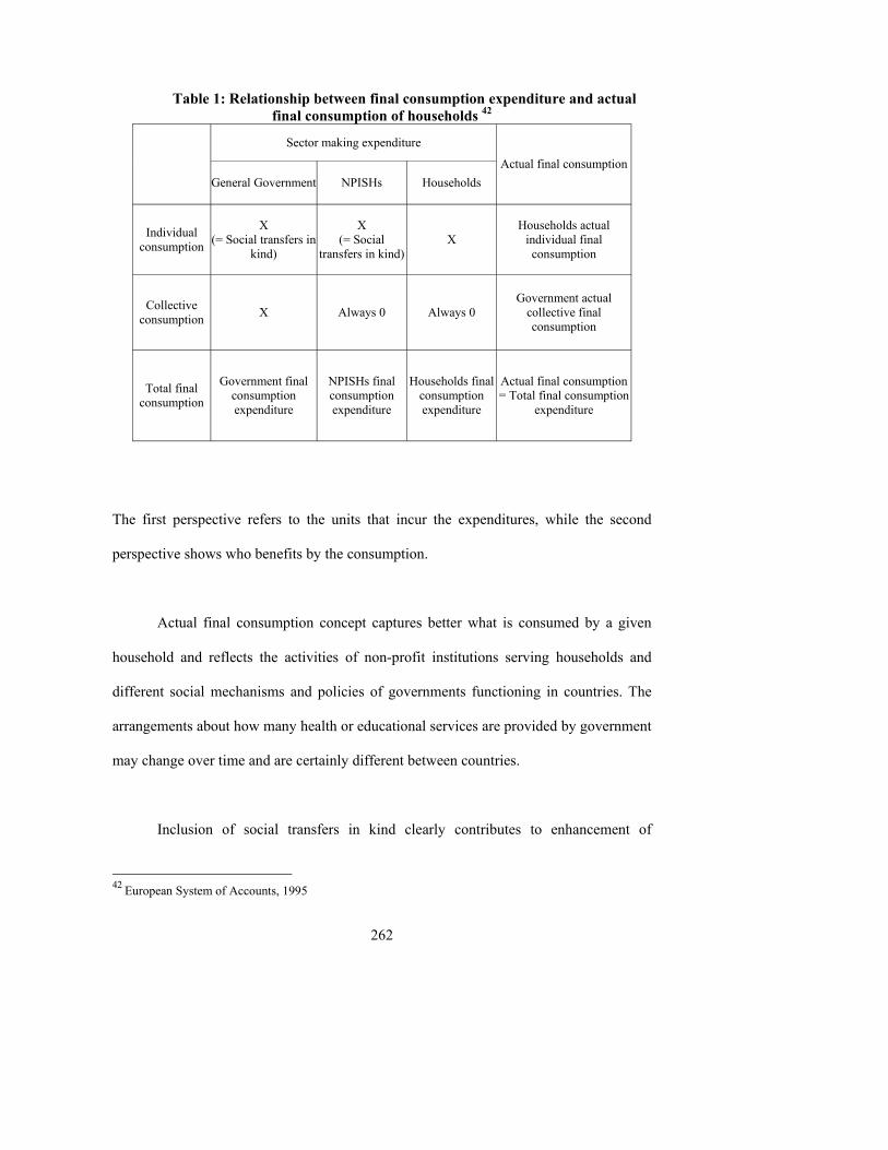
262
Table 1: Relationship between final consumption expenditure and actual final consumption of households 42
Sector making expenditure
General Government NPISHs Households Actual final consumption
Individual consumption
X (= Social transfers in
kind)
X (= Social
transfers in kind)X
Households actual individual final consumption
Collective consumption X Always 0 Always 0
Government actual collective final consumption
Total final consumption
Government final consumption expenditure
NPISHs final consumption expenditure
Households final consumption expenditure
Actual final consumption = Total final consumption
expenditure
The first perspective refers to the units that incur the expenditures, while the second
perspective shows who benefits by the consumption.
Actual final consumption concept captures better what is consumed by a given
household and reflects the activities of non-profit institutions serving households and
different social mechanisms and policies of governments functioning in countries. The
arrangements about how many health or educational services are provided by government
may change over time and are certainly different between countries.
Inclusion of social transfers in kind clearly contributes to enhancement of
42 European System of Accounts, 1995
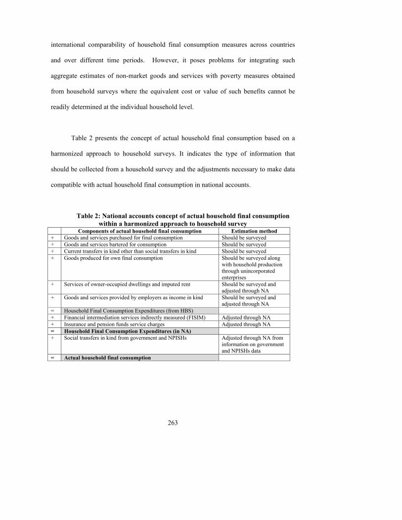
263
international comparability of household final consumption measures across countries
and over different time periods. However, it poses problems for integrating such
aggregate estimates of non-market goods and services with poverty measures obtained
from household surveys where the equivalent cost or value of such benefits cannot be
readily determined at the individual household level.
Table 2 presents the concept of actual household final consumption based on a
harmonized approach to household surveys. It indicates the type of information that
should be collected from a household survey and the adjustments necessary to make data
compatible with actual household final consumption in national accounts.
Table 2: National accounts concept of actual household final consumption within a harmonized approach to household survey
Components of actual household final consumption Estimation method + Goods and services purchased for final consumption Should be surveyed + Goods and services bartered for consumption Should be surveyed + Current transfers in kind other than social transfers in kind Should be surveyed + Goods produced for own final consumption Should be surveyed along
with household production through unincorporated enterprises
+ Services of owner-occupied dwellings and imputed rent Should be surveyed and adjusted through NA
+ Goods and services provided by employers as income in kind Should be surveyed and adjusted through NA
= Household Final Consumption Expenditures (from HBS) + Financial intermediation services indirectly measured (FISIM) Adjusted through NA + Insurance and pension funds service charges Adjusted through NA = Household Final Consumption Expenditures (in NA) + Social transfers in kind from government and NPISHs Adjusted through NA from
information on government and NPISHs data
= Actual household final consumption
264
B. Conceptual adjustments of household final consumption expenditure between household budget survey and national accounts
Conventional form of household budget survey (HBS) conducted by national
statistical offices is an important source for national accounts as it provides information
on household consumption at the lowest detailed level. This type of survey, as well as the
other varieties of household surveys like Living Standard Measurement Survey, can
furnish data on almost all the items listed above, except FISIM and insurance service
charges. Compilation of a comprehensive estimate of household consumption requires a
combination of different data sources and methods to obtain the �best estimate� for each
consumption item. Simple aggregates from HBS data cannot be directly used for national
accounts estimates of household final consumption expenditure even after verification of
the quality of those data. It is necessary to make adjustments to transform HBS data into
corresponding estimates for national accounts purposes. These conceptual adjustments
are accomplished mainly through the commodity flow approach as described and
schematically presented in Diagram 1 below.
i. Adjustments for differences in definitions and concepts Besides monetary expenditures of households, the comprehensive estimate of
household consumption requires some adjustments to account for certain imputed
expenditures on goods or services that households produce for themselves. These are
treated as expenditures because households incur costs in their production. Listed below
are imputed household expenditures recognized in the 1993 SNA.
• Household production for own final consumption - According to the 1993 SNA
recommendations, the production boundary includes goods and services created
265
for own final consumption (see endnotes for a specific discussion), except
domestic and personal services produced by members of households for
consumption by themselves or other members of the same household. The 1993
SNA further stipulates (SNA, para. 6.25) that when the amount of a good
produced within households is believed to be quantitatively important in relation
to the total supply of that good in a country, its production should be recorded.
For example, processed and consumed agricultural products by the households
could account for a significant part of the household production for own final
consumption. Processed products are classified as both output of unincorporated
activities of households and household final consumption expenditure.
• Services of owner-occupied dwellings - Persons who own the dwelling in which
they live are treated as owning unincorporated enterprises that produce housing
services consumed by the households to which the owner belongs. Housing
services produced are deemed to be equal in value to the rentals that would be
paid on the market for accommodations of the same size, type and quality.
• Income in kind - This includes goods and services received by households as
wages and salaries in kind from employers, such as free food, clothes, dwellings,
and medical attention.
• Financial intermediation services - Indirectly measured (FISIM), these should
include only the imputed service charges on the household uses of financial
266
intermediation services provided by banks, not the amount of interests paid or
received. Financial intermediaries provide services for which no explicit charges
are made. But they apply different rates of interest to borrowers and depositors.
The value of FISIM is equal to the difference between interest received and
interest paid by the financial intermediaries. In principal, FISIM should be
allocated among all institutional sectors, using these services.
• Insurance and pension fund services - For each type of insurance considered, the
gross premium consists of a service charge element and a residual element, which
is a transfer to the technical reserves. This implicit service charge is the only part
which should be recorded as a household final consumption expenditure.
However, it can only be estimated from insurance companies� accounts. HBS can
only record gross premiums at the individual level and categorize them in an
analytically-useful manner.
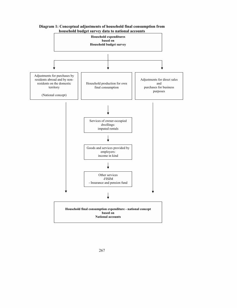
267
Diagram 1: Conceptual adjustments of household final consumption from household budget survey data to national accounts
Household expenditures based on
Household budget survey
Adjustments for purchases by residents abroad and by non-
residents on the domestic territory
(National concept)
Household production for own final consumption
Adjustments for direct sales
and purchases for business
purposes
Services of owner-occupied dwellings:
imputed rentals
Goods and services provided by employers:
income in kind
Other services -FISIM
- Insurance and pension fund i
Household final consumption expenditure - national concept
based on National accounts
268
Besides these adjustments to the basic data of HBS to meet the household-
consumption expenditure concept of national accounts, some additional conceptual issues
requiring special treatment are worth mentioning.
- Hire purchases are recorded as purchases made by the households for
the full value of the goods at the moment they take place.
- Lottery services are valued net of lottery winnings.
- Imported second-hand goods are treated in the way the newly
purchased goods are treated. In case of trading between households, no
transaction is recorded.
- Subscriptions, contributions, and dues paid by households to NPISHs
(like trade unions and professional societies) are treated as other
current transfers.
ii. Adjustment for direct sales and purchases for business purposes The HBS has certain limitations as a comprehensive data source for estimating
household expenditures. This does not imply that household surveys are not an
appropriate tool for national accounts measurement of household consumption. But since
the survey sample is usually small and the recall period short, the representativeness of
the data may be questionable. It may not properly cover expenditures on some seasonally
consumed items or on infrequently purchased durable goods. Evidence suggests that on
these latter items, a short recall period provides more robust estimates. Furthermore,
some household survey designs, gather information that does not separate expenditures
related to unincorporated activities of households. Thus, the household expenditure may
include not only spending for direct satisfaction of individual needs and wants, but also
intermediate and capital expenditures on non-durables and durables incurred for business
purposes.
269
The large share of goods (mainly agricultural) produced on own account and
consumed within the same household (after some minor processing or used fresh)
typically forms part of the consumption pattern of low-income households, especially in
rural areas. When estimating private household-consumption expenditure, home-
produced agricultural output for own consumption should be adjusted for both
intermediate use (if they are used for feeding animals or seeds for future crops
production) and for the share sold directly on the market or bartered between households.
National accountants accord particular attention to these goods since they could be
equally used for final or intermediate consumption. Costs of producing them are borne by
the households themselves and might not be shown explicitly in the surveys. But they
should be estimated and deducted so that the private household-consumption expenditure
and the corresponding poverty measure will not be affected.
iii. Adjustments for purchases by residents abroad and non-residents residing in domestic territory
Household final consumption expenditure in the 1993 SNA refers to expenditures
incurred by resident households within the economic territory and abroad. This approach
means household final consumption expenditure should be adjusted to meet the
recommended national concept of its recording, i.e., expenditures of resident households
made abroad should be included while expenditures of non-resident households in the
domestic territory should be excluded from the estimate. Monetary expenditures of non-
residents are recorded as exports of goods and services on the revenue side of the Balance
of Payments. Monetary expenditures of residents abroad are recorded on its expenditure
270
side as imports of goods and services.
In this context, persons going abroad for short periods (less than one year) and
foreign students, patients, and diplomats and their dependants (irrespective of their
duration of stay) are considered residents of their home countries; their consumption
expenditures are part of their home economies. Implication of this rule is that where a
low-income country is a tourist destination, extra care has to be taken in the national
accounts to ensure foreign visitors� expenditures are not incorporated within the
aggregate consumption estimates. This issue does not arise in household survey
measures.
C. Empirical adjustments of household-consumption expenditure between household budget surveys and national accounts
In addition to the conceptual adjustments mentioned above, empirical adjustments
are needed with respect to use of additional source data and adjustment for non-observed
household activities, described in Diagram 2 below.
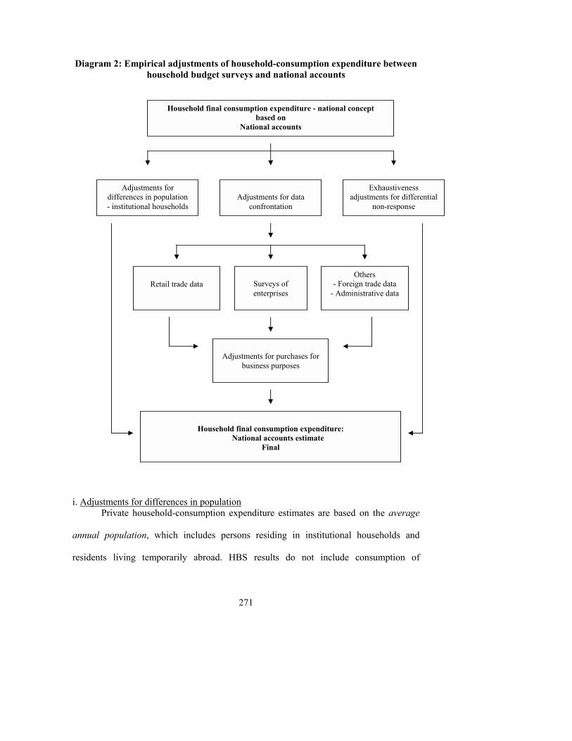
271
Diagram 2: Empirical adjustments of household-consumption expenditure between household budget surveys and national accounts
i. Adjustments for differences in population
Private household-consumption expenditure estimates are based on the average
annual population, which includes persons residing in institutional households and
residents living temporarily abroad. HBS results do not include consumption of
Household final consumption expenditure - national concept based on
National accounts
Adjustments for differences in population - institutional households
Adjustments for data
confrontation
Exhaustiveness adjustments for differential
non-response
Retail trade data
Surveys of enterprises
Others - Foreign trade data
- Administrative data
Adjustments for purchases for
business purposes
Household final consumption expenditure:
National accounts estimate Final
272
institutional households. National accounts usually provide supplementary estimates on
consumption of persons living in institutions on the basis of information from additional
data sources, by using administrative records of the institutions or, more implicitly, by
using retail trade statistics used for adjusting the HBS data. This concerns mainly the
consumption of individuals residing in old people�s homes, institutions for the disabled
and mentally ill, hospices, and inmates of prisons.
ii. Exhaustiveness adjustments and differential non-response rates HBS data has certain weaknesses, including low representation of high-income
households. Affluent households often refuse to participate in the survey. As a result,
this leads to underestimates of household final consumption expenditure. Appropriate
adjustments, relying on grossing up techniques, are undertaken to reflect higher-income
household expenditures and to improve HBS results. Although this adjustment will not
affect the consumption of the poor households, it will affect the distribution of
consumption and the survey mean if the adjustments are imputed back into the survey
data. Otherwise, if this adjustment is only made in the national accounts, significant
differences between the survey and national accounts means in consumption will occur.
iii. Additional data sources used for measuring household final consumption expenditure Data confrontation and reconciliation are at the core of national accounts
compilation practice. They are not specific only to the estimation of private household
consumption expenditure. In national accounts practice, HBS results are not used for
estimation of every single item of expenditure. Rather, they are used selectively, based on
their quality and the availability of alternative data sources. HBS results tend to
underestimate expenditures on certain items, like alcohol, tobacco, and some personal
services. For these reasons, in addition to HBS data, national accounts draw on retail
273
trade data and other statistics based primarily on tax, output, and import information
when estimating these items. No one source can be considered entirely adequate. Final
data for household final consumption expenditure are derived through the commodity-
flow approach within a supply and use framework, i.e., detailed and specific adjustments
are made at the lowest possible level of commodity use and aggregation. See Endnotes
for further discussion of Retail Trade data and Surveys of Enterprises.
iv. Additional adjustments and considerations for exhaustiveness in using HBS data for national accounts purposes
Activities in the non-observed economy may play a very important role in
determining both income and expenditure data of HBS and household final consumption
expenditure estimates in the national accounts. Non-observed activities may give rise to
imbalances in the basic data and resulting estimates, but conversely, such data imbalances
may provide evidence of non-observed activities and the significance of the grey
economy.
Households that are especially active in the informal economy and not fully
reporting their incomes for tax or statistical purposes might form a disproportionate share
of those who refuse to participate in the survey. Although it is impossible to determine
the precise extent to which non-observed activities could affect consumption
expenditures, many statistical offices are constantly making efforts to obtain better and
more exhaustive estimates by applying the different approaches recommended in the
OECD handbook, �Measuring the Non-Observed Economy.�
Frequency and timelines with which household surveys are carried out can have
an important impact on the quality of HBS data. Continuous surveys provide time series
274
for individual items of expenditure and significantly enhance the quality of estimates.
Timeliness means that HBS data can potentially be used as a prime source for national
accounts purposes. Timeliness also increases the frequency in which data can be
validated against other sources. These two characteristics are simultaneously required.
Unfortunately, many developing countries carry out a HBS at infrequent intervals,
some that exceed five years. This necessitates implementation of extrapolation techniques
and interpolation for the estimation of household final consumption expenditure for the
years in between surveys. Considerations regarding the relatively short recall period of
the household surveys and lengthy time for data processing play an important role in the
quality and reliability of national accounts estimates.
In the absence of external support, financial constraints and real resource
difficulties faced by many developing countries often compel them to adopt relatively
small samples or to restrict a HBS to urban areas. Omission of rural household
expenditures, which may reveal a different consumption pattern over a more limited set
of goods and services, distort the ability of HBS data to represent the national condition,
especially pertaining to consumption items. Generalization of sample data over the total
population without any adjustments for coverage may result in misrepresentation of
household final consumption expenditure.
275
6.8 Mapping Poverty Characteristics
6.8.1 Piecing the puzzle together
After gathering all forms of data from different sources and establishing a variety
of definitions and classifications, it remains a challenge to overlay the various pieces of
information using both proximate and exact matching techniques related to households.
The socio-economic groups to which households belong and their links to specific places
of habitation and location are rarely clear, This makes it difficult to meaningfully order
all geographically-related data required to paint the more comprehensive picture
decision-makers seek.
Researchers are increasingly attempting to link micro household or product data
obtained from surveys and small area studies with a comprehensive database developed
from a census. Compilation of this �map� requires �bootstrapping� and other data mining
techniques. �Sound procedures� for interpolating and extrapolating figures and for
generating retrospective estimates of benchmark data have to be put in place. Their
validity will depend on the availability of relevant proxy series and other related
indicators that are available. These indicators would normally include appropriate price,
output, wage and employment series, and sales measures that suitably reflect the options
and boundaries that constrain household decisions. Use of any series to move estimates in
different directions from a given observation will suffer, however, from adoption of the
structural fixity embedded in the benchmark reference. Accordingly, they may not be
276
able to capture the effect relative price changes have on product substitution and
emerging consumption patterns as new products and services enter the market.
Pioneering work in this area of social mapping was conducted by the North West
Regional Health Authority in England when it linked graphically where people lived
[urban industrial locations and rural agricultural areas] with their assumed socio-
economic status, individual occupational category, industry of employment and the
incidence of various diseases and health indications. Apart from the intention to say
something about social class, a pattern emerged showing clear relationships between
different social groups and their exposure to environmental hazards. This highlighted
individuals� risk of contracting certain medical ailments based on his or her occupation
and living conditions, such as having open hearth coal fires in the house and type of diet.
A similar post-enumeration study in China linked income data from the latest
household survey with data from the household-based First Agricultural Census of China
[1997-1999] to determine levels of well-being across provinces. The aim was to see how
income levels could be related to the type of economic and farming activity in those
areas. The results showed that the traditional grain producers found mostly in the north
and north-western provinces were especially vulnerable to low and fluctuating incomes,
and that they had the fewest opportunities to bring in additional income from non-farm
activities located in nearby urban areas. This adversely affected educational
opportunities, diet of their children, and overall household nutrition.
277
Ideally, the data used to compile these more complete pictures should be based on
the respective benchmark and survey information relating to the same households. But
this approach would probably yield too few matches and result in significant bias. Thus,
the characteristics of similar households engaged in different surveys or in different
rounds of the same survey are usually combined to produce a more complete picture.
Problems of area sampling and following through in this process to achieve lower
levels of disaggregation have been described in Chapters 5 and 7 in this handbook. Panel
studies that track the activities and characteristics of the same households over a long
period of time suffer from individual attrition and aging which alters the nature and
composition of households (See Chapter 8 for more discussion on data). Surveys are
compromised by their inability to sustain �like with like� comparison and to hold certain
factors constant. To extract and uproot more detailed micro information embedded in
national and other statistical aggregates (e.g., final household consumption expenditures
and rural subsistence output) demands prior data about target groups and those at risk -
and where these people can usually be found. But the results can cast new light on old
problems.
278
6.8.2 Drawing on appropriate indicators
Different indicators exist in the public domain that can approximate information
about the comparative status and economic level of households. Related structural
indicators can help monitor changes in those levels. Synthetic and composite indices that
measure national well-being [e.g., the UNDP Human Development Index] use common
data and adopt recognized statistical procedures across each country to provide a wider
perspective of the relative standing of various socio-economic groups and their progress.
Such index measures are not precise nor independently verifiable. They are best
employed in making ordinal rather than cardinal assessments. Although appealing to no
underlying social logic relevant to the scale transformations and aggregations carried out,
there is a high correlation between many individual component indices depicting growth,
levels of living and social progress. However, composite index numbers, while useful as
broad indicators of overall well-being, do not rest on any inherent conceptual basis. They
are therefore limited and not very robust for comparative inter-country and inter-temporal
purposes.
Many composite measures, while superficially relating to the multiplicity of
dimensions implicit in the inherent individual indices, have little relevant appeal to an
intrinsic social or economic body of thought. There is little rationale, other than
arithmetic transparency, to support the simple weighting procedures adopted for
aggregating component indices. Some carefully constructed synthetic or composite
279
measures may provide, nevertheless, a reasonable indication as to the overall competence
of governments and reflect the basic quality of governance and the efficacy of their social
delivery mechanisms.
6.9 Conclusion
This chapter has looked at different data collection techniques and reviewed the
possibility of combining various types of information from alternative sources to provide
more insightful poverty assessments. Emphasis is on the need to fuse qualitative and
subjective methods with the more traditional official baseline data collections. As part of
a more comprehensive probability-based survey design, such approaches can be very
informative in amplifying the raw numbers. Relying on data compiled for different
purposes to paint a broader canvas, however, does not necessarily provide the specific
information required for the range of poverty analysis many policy makers need. This is
especially so when there is a desire to break down the information by provinces and
regions. A better approach might be to devise a grand survey design that incorporates the
potential to carry out planned studies based on evolving small area statistical estimation
techniques.
Quite apart from the difficulty of linking and cross-validating information of
various qualities from different sources, the proper choice of what data to bring to bear on
280
an issue poses questions of specificity versus consistency and representation versus
comparability. These issues affect the choice of data necessary to monitor and evaluate
the nature of poverty in a uniform and consistent manner. In this respect, when
comparing values, price differences according to location and various types of outlet
assume considerable significance. Such pricing questions must also be taken into account
when considering how best to preserve the temporal and spatial consistency of poverty
estimates and whether a special exercise is necessary to determine whether the poor are
paying prices that are markedly different than those paid by the broader community.
Several general themes run through the above discussion.
• A large sample size for a household survey--necessary for a more
detailed level of disaggregation and the simultaneous study of multiple
topics--adds significantly to survey costs. It also leads to potentially
large non-sampling errors. Survey managers are thus under pressure to
find alternative and cheaper means �to fill in the gaps.� If such
methods also expand the knowledge about poverty and track changes
in household and individual levels of living as they occur over time, so
much the better.
• A more complete understanding of the complexity of poverty requirers
researchers to go beyond mere collection of income and expenditure
numbers obtained in a conventional household survey, regardless of
how representative it might be of the total population.
281
• It is important to strive for consistency across regions to allow for
comparisons between different communities within each country. This
is not only a matter of following the same data collection methodology
but also ensuring that the measures themselves are relevant and
consistent. In assessing living conditions of poor households, it�s
essential to know the actual physical quantities obtained (such as how
much food they get) as well as the value of outlays they have made.
Here again, this is not easy if prices for specific items vary
significantly over time, as well as between different locations and
outlets within a country.
Many country- and community-based poverty evaluation and monitoring systems
lack consistency because they are launched by donors and external agencies possessing
the necessary seed funds but lacking concern for a coordinated focus. They do not usually
fit together in terms of their scope, timing and coverage. Many will have been
implemented as one-off exercises or prove unsustainable for either technical or financial
reasons.
The aims and methods of such surveys are quite different from the procedures
observed by the national statistical office. Desire for basic coherence also requires the
complete methodological consistency between countries. Achieving this standard is one
of the main purposes of the present handbook.
282
Furthermore, long-term trend analysis within a given country requires adherence
to the original benchmark and survey design wherever possible. This implies using the
same array of indicators for updating trends, even if the procedure is less than optimal
and if new methods are subsequently found. These can always be updated with the next
round of benchmark studies. While clearly challenging, it is critical for researchers to
find the appropriate balance between these competing ends and undertake a robust
temporal and spatial analysis.
There are, nonetheless, certain questions that still evade quick and easy resolution.
For one, a distinction cannot be readily drawn, simply from a standard cross section
study, between chronic and transient poverty even with access to an array of
supplementary data. While basic conditions of poverty are a legacy handed down from
one generation to the next, many households will pass through various phases of being
poor during their lifetime.
Availability of sequential data from longitudinal studies and time-related
indicators may suggest solutions to policy makers about how poor households escape
from poverty over time. Such time series data can reveal how changes in the
circumstances of individual households and changes in the actual size and composition of
the household, particularly its age and sex profile, can affect the daily living standards of
its members.
283
Another key issue is that the record of expenditures compiled in a household
survey implicitly assumes that the relative importance of any item is dependent on the
simple share of the weekly or monthly budget that households spend on it. These surveys
rarely take into account the question of priorities and the need for people to meet certain
mandatory obligations when making their regular outlays. Importance of food,
paradoxically, is frequently subsumed to that of shelter. Regular outlays on both have to
give way to community charges and other unavoidable local fees, trade credit obligations,
and protection payments. The occasional need to pay certain national statutory �poll�
taxes and repay personal debts to friends and relations are additional priorities.
The virtue of engaging different methods of inquiry to present a broad holistic
picture that can simultaneously draw attention to details having a distinct bearing on the
question under review (but which might otherwise have been overlooked), is
indisputable. The actual act of researchers and officials in applying these methods and
imputation techniques may have important and desirable feedback implications for the re-
design of selected administrative records. It can also influence the choice of the
qualitative survey approaches that could contribute to the creation of a more complete
picture of poverty and its relationship to other social problems.
284
If carefully assessed and evaluated, the availability of more rather than less
information will invariably contribute to a better understanding of poverty�s multi-
dimension character. The key is selecting and integrating the appropriate sources and
series to match available data that address the essential broad issues.
Direct estimation of household final consumption expenditure (in contrast with its
derivation as a residual) using several completely independent data sources has clear
preference over single-source estimates. Having more than one estimate for the different
expenditure items allows for comparative analysis and evaluation of quality and
reliability. Comparative evaluation of conceptual and empirical differences and
subsequent adjustments would improve the quality and reliability of the national accounts
estimate for household final consumption expenditures as compared with a single-source
estimate obtained from HBS expenditure data. Therefore, countries should be encouraged
to apply statistical reconciliation (adjustment) techniques in deriving harmonized
consumption expenditure averages for national accounts and HBS data in the broader
contextual analysis of poverty. Furthermore, conceptual and empirical differences and
adjustments between household surveys and national accounts data should explicitly
consider the impact of these adjustments on income/consumption distribution across
households for which the household survey is the only tool that can provide this
information for the purpose of measuring poverty.
Household surveys need to be improved in many countries. They must make use
of the extensive experience accumulated over the past decades in such areas as,
285
• Representative sample design, • Consistency of forms and methods of data collection over time, • Formulation of questions and coverage of data items, and • Proper training of interviewers to reduce unit and item non-response and other
non-sampling errors.
Notwithstanding, international agencies and other organizations should give high priority
to developing global household survey standards to generate reliable poverty estimates
consistent with the national accounts across countries and across time. As such,
harmonized household surveys would encourage counties to adopt a direct measure of
household consumption in national accounts.
286
ENDNOTES
E.1. Social transfers in kind (SNA, para. 9.72)
Social transfers in kind include: - Individual goods or services produced or purchased by the government and
NPISHs and distributed free or below market cost to individuals, such as education,
health, social security and welfare, sports and recreation, culture, part of provision of
housing, collection of household refuse, and operation of transport;
- Social benefits in kind include reimbursements from government�s social
security funds to households on specified goods and services bought by households on
the market;
- Other social security benefits in kind are also counted, except reimbursement
which are not produced by the government sector but bought and distributed free or
almost free to households under the social security funds; and
- Social assistance benefits in kind, including the free distribution of food and
clothing
E.2. Household production for own final consumption It includes:
- Agricultural products and their subsequent storage;
- Gathering of berries or other uncultivated crops;
287
- Forestry;
- Wood-cutting and the collection of firewood; hunting and fishing;
- Production of other primary products such as mining salt, cutting peat, and
water;
- Processing of agricultural products;
- Other kinds of processed goods, such as weaving cloth, dress making, and
tailoring; and
- Own account fixed capital formation.
Other household production of services like cleaning, cooking, transportation, and the
caring for children, and sick and old household members are outside the production
boundary with two exceptions � services of paid domestic staff and imputed rent of
owner-occupied dwellings. (SNA, para. 6.24)
E.3. Additional data for measuring household final consumption
Retail trade data constitute a more reliable source of information concerning
consumption of alcohol, tobacco, and durables compared with the HBS results. If
available at a detailed level, they are an important tool for verifying HBS data for many
groups of non-food commodities. Retail surveys also cover consumption of institutional
households and consumption of non-residents [but usually without distinction] on
domestic territory, i.e., retail trade surveys present results in accordance with the
domestic concept in national accounts.
288
The major problem with retail trade data is that they include sales to units other
than households, i.e., purchases for business purposes, which should be excluded to
achieve the 1993 SNA compliant estimate of household final consumption expenditure. If
retail trade data are used independently and not constrained by other available sources for
estimation of household consumption, they may underestimate expenditures of some
commodities as households also purchase goods directly from producers or other
households. At the same time, they may overestimate consumption of other households
because purchases for intermediate consumption have not been excluded.
Surveys of enterprises are the other important data source providing information
on the value of electricity and water purchased by households as well as transport,
communication, and personal services provided. The main practical difficulty with
enterprise data is the same as with retail trade data � they include business consumption,
which should be excluded.
289
References Anand Sudhir (1993) and Ravallion Martin, (1993), Human Development in Poor Countries: On the Role of Private Incomes and Public Services, The Journal of Economic Perspectives, Vol.7, No., pp 133-150 Carvalho Soniya and White Howard, (1996), Combining Qualitative and Quantitative approaches to Poverty Measurements and Analysis, World Bank Technical Paper No. 366, Washington DC, The World Bank CBS- Statistics Netherlands, (2004), The poor Side of the Netherlands: Results from the Dutch Poverty Monitoring 1997-2003 Chambers Robert, (1994), The Origins and Practice of Participatory Rural Appraisal, World Development, Vol. 22, No. 7, pp 953-969 Deaton, Angus (2000), �Counting the world�s poor: problems and possible solutions�: Research Program in Development Studies, Princeton University Deaton Angus (2003), How to Monitor Poverty for the Millennium Development Goals, Journal of Human Development, Vol. 4, No. 3 (2003), pp 353-378 Deaton, Angus (2003), �Measuring poverty in a growing world (or measuring growth in a poor world): BREAD Working Paper No. 036, Bureau for Research in Economic Analysis of Development Fuentes, Ricardo and Montes, Andres (2004), Mexico and the Millennium Development Goals at the Subnational Level, Journal of Human Development, Vol. 5, No. 1, March 2004, pp 97-120 Grosh Margaret and Glewwe Paul (1996), Household Surveys from Developing Countries � Progress and Prospects, International Macro- and Microeconomic data: Reliability, Comparability, and Adequacy-AEA Papers and Proceedings, Vol. 86, No. 2 (1996), pp 15-19 Hanmer Lucia, Pyatt Graham and White Howard (1999), What do the World Bank�s Poverty Assessments teach us about Poverty in Sub-Sahara Africa? Development and Change, Vol. 30 (1999), pp 795-823 Hanmer Lucia, Lensink Robert and White Howard (2003), Infant and Child Mortality in Developing Countries: Analysing the Data for Robust Determinants, The Journal of Development and Studies, Vol. 40, No.1, (October 2003), pp 101-118 Karshenas, Massoud (2003/49), �Global poverty: National accounts-based versus survey-based estimates�, Employment Papers, Employment Sector, International Labour Office, Geneva
290
Karshenas, Massoud (2004/5), �Global poverty estimates and the millennium goals: Towards a unified framework�: Employment Strategy Papers, International Labour Office, Geneva King A. Loren (1998), Economic Growth and Basic Human Needs, International Studies Quarterly, 42, pp 385-400 Laderchi C. Ruggeri, Saith Ruhi and Stewart Frances, 2003, Does it Matters that we do not Agree on the Definition of Poverty? A comparison of four Approaches, Oxford Development Studies, Vol. 31, No. 3, September 2003 Pyatt Graham and Ward Michael (1999), Identifying the Poor, IOS Press Ravallion, Martin (1992): �Poverty Comparisons; A guide to concepts and Methods� The World Bank Ravalion Martin (1996), Issues in measuring and Modeling Poverty, The Economic Journal, Vol. 106, No 438 (Sep., 1996), pp 1328-1343 Ravallion, Martin (2003): �The Debate on Globalization, Poverty, and Inequality: Why Measurement Matters� Policy Research Working Paper 3038, The World Bank Ravallion, Martin (2003): �Have We Already Met the Millennium Development Goal for Poverty? Ravalion Martin and Sen Binayak (1996), When Methods Matters: Monitoring Poverty in Bangladesh, Economic Development and Cultural Changes, Vol. 44, No 4 (July., 1996), pp 761-792 Sen Amartya (1998), Mortality as an indicator of economic success and failure, The Economic Journal, Vol.108, No. 446 (January), pp 1-25 Shaffer Paul (1996), Beneath the Poverty Debate, Some Issues, IDS Bulletin, Vol. 27, No 1 Surjit, Bhalla, 2002, �Imagine There�s No Country: Poverty, Inequality, and Growth in the Era of Globalization�, Washington: Institute for International Economics
System of National Accounts, 1993, United Nations, Series: F, No.2 European System of Accounts, 1995, Eurostat
291
Teekens Rudolf, Van Praag Bernard (1990); Analyzing poverty in the European Community: Policy issues, research options, and data sources; pp 449 World Bank (1994) Zambia. Poverty Assessment, Grey cover report No. 12985-ZA. Washington, DC: The World Bank World Bank (1995a) Ghana. Poverty Past, Present and Future, Grey cover report No. 14504-GH. Washington, DC: The World Bank World Bank (1995b) Kenya. Poverty Assessment, Grey cover report No. 13152-KE. Washington, DC
292
CHAPTER VII. POVERTY ANALYSIS FOR POLICY USE: POVERTY PROFILES AND MAPPING
Nanak Kakwani and Hyun H. Son43
Introduction
This chapter focuses on the formulation of poverty reduction policies. It shows
how various poverty tools can be of considerable value to policy makers in strengthening
the poverty alleviation impact of government spending. Poverty profiles can play an
important role in understanding poverty and formulating poverty reduction policies. In
this chapter, we provide some country specific examples to illustrate how poverty
profiles can be constructed and how they can be utilized to design policies.
The primary step in determining the degree of poverty is establishing a poverty
line that specifies in monetary terms a society�s judgment regarding the minimum
standard of living to which everybody should be entitled. Once the poverty line is
determined, one can construct poverty profiles, which provide overall estimates of
poverty, distribution of poverty across sectors, geographical regions and socioeconomic
groups, and a comparison of key characteristics of the poor versus non-poor.
43We are thankful to Fabio Soares for his helpful comments.
293
The method of setting the poverty line can greatly influence poverty profiles,
which are the key to the formulation of poverty reduction policies. Unfortunately, setting
a poverty line is not a straightforward exercise; indeed, it is often a very contentious
exercise. Setting a poverty line involves many conceptual and practical problems. These
are critical from the point of view of policy development, but they are often ignored due
to their complexity. This matter has been dealt with in great detail in Chapters 3 and 5.
Once researchers define the poverty line, then they can calculate the number and
percentage of poor in the country. These are estimates of incidence of poverty, which are
obtained under the assumption that if a household is identified as poor, then all its
members are also poor. These poverty estimates provide no information about the depth
of poverty. One index of poverty that does take account for the depth of poverty is the
poverty gap ratio. This index captures the depth of poverty by contrasting the mean
income (or consumption shortfall) relative to the poverty line, averaged across the whole
population44. Thus, this measure gives us an idea about the total resources required to
bring all the poor up to the poverty line.
Finally, there is another index of poverty called the severity of poverty, which
takes into account not only the depth of poverty but also inequality of income or
consumption among the poor. This index helps officials focus policies on eliminating
44 When establishing this mean, the non-poor are assigned a poverty gap of zero.
294
extreme or ultra poverty by giving greater weight to the income or consumption shortfalls
of the very poor45.
Geographical targeting is also becoming an important means for channeling
public resources to the poor. Many governments use it to target programs, such as food
aid, public works, and delivery of health care and education. This approach is commonly
referred to as �poverty mapping.� This chapter provides a brief review of methodology
used in the construction of poverty maps. It also points out the effectiveness and
limitations of poverty mapping.
7.1 Poverty monitoring and poverty profiles
The three poverty indices discussed in the previous section are often used as a tool
to monitor poverty over time at the aggregate level. Needless to say that monitoring
poverty at the aggregate level is important because policy makers want to know if the
government policies are helping the poor. Thailand has been monitoring poverty for more
than a decade. It has a nutrition-based official poverty line, which can be used to
calculate the three poverty measures. Figure 1 presents these estimates covering the
period from 1988 to 2002. All three poverty measures show a parallel decline in poverty
from 1988 to 1996, followed by a sharp increase through 2000 and then a sharp decrease
until 2002.
45 There is a huge range of literature on poverty measures. The most important papers among them are those by Sen (1976), Kakwani (1980), and Foster, Greer and Thorbecke (1984). The three poverty measures discussed above are the particular members of the Foster, Greer and Thorbecke�s poverty measures, which are most widely used.

295
During Thailand�s rapid growth period (1988-96), when the incidence of poverty
declined very rapidly, poverty decreased at a much slower rate when measured by the
poverty gap ratio and severity of poverty. This implies that the benefits of growth
accruing to ultra-poor were lower than those to the poor.
During the stagnation crisis between 1996 and 2000 the headcount measure
showed a much higher rate of poverty increase than the poverty gap ratio and severity of
poverty index. This means that the ultra poor suffered relatively less than the poor during
the crisis. During the recovery period, the ultra poor benefited relatively less than the
poor.
Source: Authors� calculations based on Thailand�s Socio-Economic Surveys.
Poverty profiles show how poverty varies by geography and subgroups across
society. Study divisions include regions, communities, sector of employment, and
household size and composition. Profiles can also show how rates of economic growth in
1988 1990 1992 1994 1996 1998 2000 20020
5
10
15
20
25
30
35
Incidence
gap
Severity
Figure 1: Poverty in Thailand: 1988-2002
296
different sectors and regions affect aggregate poverty. Accordingly, poverty profiles are
extremely useful in formulating the most effective economic and social policies to
combat poverty. They identify regional location, employment, age, gender and other
characteristics of the poor. This information can be used to formulate poverty alleviation
policies. Profiles can also help answer a wide range of questions such as:
• Who are the poor?
• Where do they live?
• What do they do?
• On what sectors do they depend for their livelihood?
• Do they have access to economic infrastructure and support services such as social services and safety nets? And,
• How can the government target resources to them?
The three poverty measures--incidence of poverty, poverty gap ratio and severity
of poverty--are constituents of the Foster, Greer and Thorbecke poverty indices, which
have an attractive property of being additively decomposable poverty measures (see
Chapter 3). This property can be quite useful in analyzing poverty profiles. For example,
suppose that the population is divided into K mutually exclusive groups, and let ak be the
population share of the kth group. Any FGT poverty measure, denoted by FGTα is
additively group decomposable because one can write it as:
FGTα = ∑=
K
kka
1FGTα,k (1)
297
where FGTα,k is the poverty measure for the kth group (Foster, Greer and Thorbecke,
1984). This implies that total poverty is a weighted average of poverty levels in all
groups--the weights being proportional to the groups� share of the population.
Additively decomposable poverty measures allow one to assess the effects of
changes in group poverty on total poverty. When incomes in a given group change, then
group and total poverty move in the same direction. Increased poverty in a group will
increase total poverty at a rate given by the group�s population share ai ., The larger the
population share of the group, the greater the impact will be. Equation (1) shows that
kk FGTa ,α multiplied by 100 identifies the percentage contribution of the kth group to
total poverty. This suggests that complete elimination of poverty within the kth group
would lower total poverty by this percentage. This property is desirable for evaluating
anti-poverty policies.
Table 1 presents a spatial profile of poverty in Thailand in 2000. Poverty in the
country varies rather dramatically by region. All three poverty measures indicate that the
Northeast is the poorest region, followed by the Northern, Southern, and Central regions,
and then by Bangkok. However, there is a huge regional concentration of poverty in
Thailand. The Northeast region, with one-third of the country�s population, accounts for
more than 61 percent of the country�s poor. When we measure poverty by the severity
index, the contribution of Northeast to the total poverty is even higher--nearly 65 percent.
This is in stark contrast with the capital region, the Bangkok metropolitan area, where the
country�s poverty is lowest.
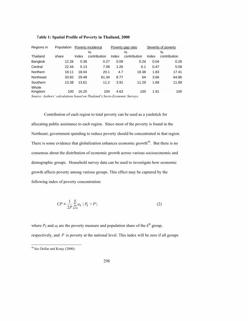
298
Table 1: Spatial Profile of Poverty in Thailand, 2000
Regions in Population Poverty incidence Poverty gap ratio Severity of poverty
Thailand share Index % contribution Index
% contribution Index
% contribution
Bangkok 12.26 0.36 0.27 0.09 0.24 0.04 0.26 Central 22.44 5.13 7.08 1.26 6.1 0.47 5.58 Northern 18.11 18.04 20.1 4.7 18.38 1.83 17.41 Northeast 33.82 29.48 61.34 8.77 64 3.66 64.86 Southern 13.38 13.61 11.2 3.91 11.29 1.69 11.89 Whole Kingdom 100 16.25 100 4.63 100 1.91 100 Source: Authors� calculations based on Thailand�s Socio-Economic Surveys.
Contribution of each region to total poverty can be used as a yardstick for
allocating public assistance to each region. Since most of the poverty is found in the
Northeast, government spending to reduce poverty should be concentrated in that region.
There is some evidence that globalization enhances economic growth46. But there is no
consensus about the distribution of economic growth across various socioeconomic and
demographic groups. Household survey data can be used to investigate how economic
growth affects poverty among various groups. This effect may be captured by the
following index of poverty concentration:
∑ −==
K
kkk PPa
PCP
1||
21 (2)
where Pk and ak are the poverty measure and population share of the kth group,
respectively, and P is poverty at the national level. This index will be zero if all groups
46 See Dollar and Kraay (2000).
299
have same poverty. The higher the value of CP, the greater is the concentration of
poverty. A value of 1 for CP implies extreme concentration of all poverty in a single
group when the number of groups goes to infinity.
Table 2: Concentration of Poverty in Thailand
Period Poverty
Incidence Poverty Gap
ratio Severity of
poverty 1996 0.22 0.22 0.23 1998 0.15 0.20 0.24 2000 0.27 0.29 0.29 2002 0.26 0.26 0.27
Source: Authors� calculations based on Thailand�s Socio-Economic Surveys
Table 2 shows that the concentration of poverty in Thailand declined sharply
during the period between 1996 and 1998 (with exception of severity of poverty, which
affects the ultra-poor more than the poor.) This is consistent with the fact that the initial
impact of the 1997-98 economic crisis was most severe in Bangkok.47 In the subsequent
period of 1998-2000, the impact of the economic crisis reverberated across the country,
triggering a greater increase in poverty in poorer regions. Thus, there was a huge increase
in the concentration of poverty. Concentration of poverty continued to be high during the
recovery period between 2000 and 2002; the country�s poorer regions did not benefit
from recovery as well as the richer regions.
These poverty profiles capture the regional inequities in Thailand. Division of the
population into groups need not be done only in terms of geographical regions. Groups 47 Since the Bangkok Metropolitan is the richest region, any increase in poverty in the region will reduce the concentration of poverty.
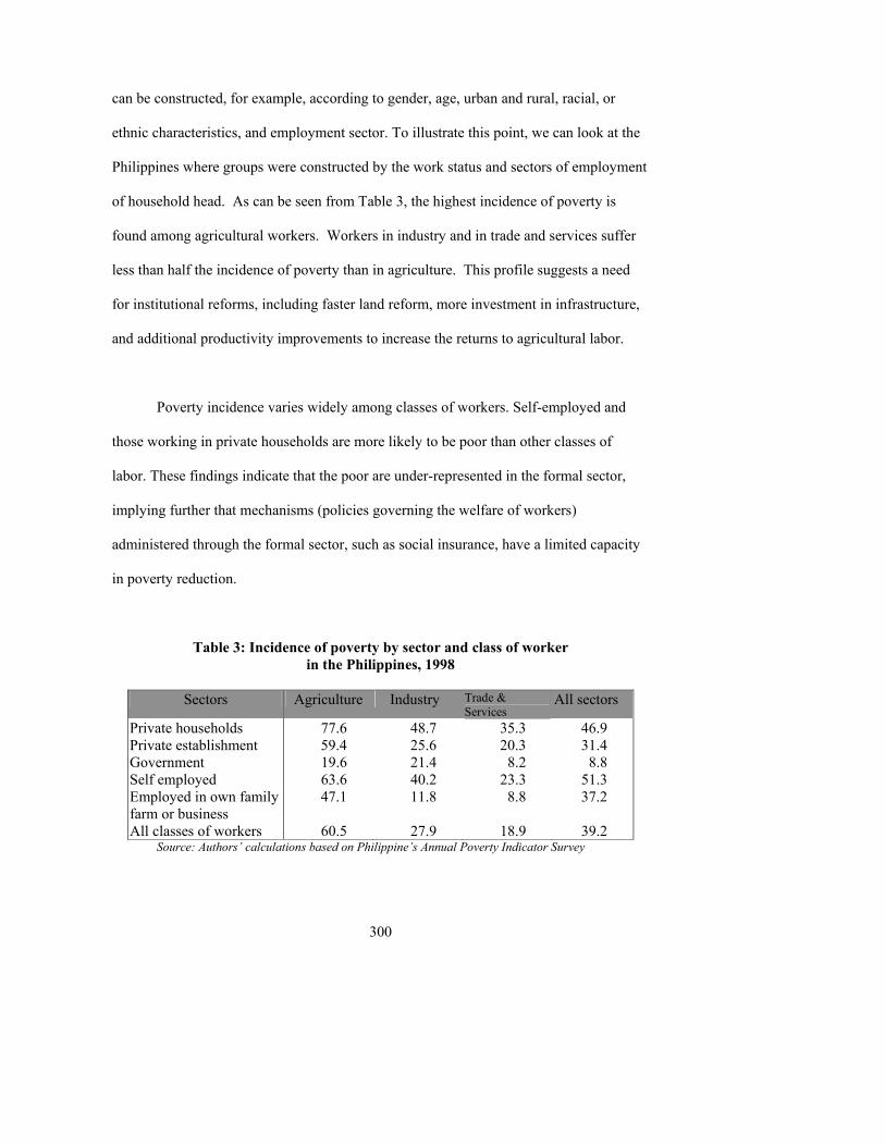
300
can be constructed, for example, according to gender, age, urban and rural, racial, or
ethnic characteristics, and employment sector. To illustrate this point, we can look at the
Philippines where groups were constructed by the work status and sectors of employment
of household head. As can be seen from Table 3, the highest incidence of poverty is
found among agricultural workers. Workers in industry and in trade and services suffer
less than half the incidence of poverty than in agriculture. This profile suggests a need
for institutional reforms, including faster land reform, more investment in infrastructure,
and additional productivity improvements to increase the returns to agricultural labor.
Poverty incidence varies widely among classes of workers. Self-employed and
those working in private households are more likely to be poor than other classes of
labor. These findings indicate that the poor are under-represented in the formal sector,
implying further that mechanisms (policies governing the welfare of workers)
administered through the formal sector, such as social insurance, have a limited capacity
in poverty reduction.
Table 3: Incidence of poverty by sector and class of worker in the Philippines, 1998
Sectors Agriculture Industry Trade &
Services All sectors
Private households 77.6 48.7 35.3 46.9 Private establishment 59.4 25.6 20.3 31.4 Government 19.6 21.4 8.2 8.8 Self employed 63.6 40.2 23.3 51.3 Employed in own family farm or business
47.1 11.8 8.8 37.2
All classes of workers 60.5 27.9 18.9 39.2 Source: Authors� calculations based on Philippine�s Annual Poverty Indicator Survey
301
Although poverty profiles are very useful in understanding the nature of poverty,
they are limited to showing bivariate associations between various socioeconomic groups
and poverty measures. In other words, they do not control for other omitted variables,
which also have an impact on poverty. In many instances, this profiling approach can
generate misdirected policies. To illustrate this point, it may be useful to mention Pyatt�s
(2000) example of Malaysia, where the data confirmed that poverty was associated with
ethnicity so the main strategy of the government to reduce poverty was to redistribute
wealth to Malays. However, the data also suggested a rural/urban correlation to living
standards and educational attainment within the household. When all three typologies
were analysed simultaneously, the ethnic dimensions were no longer significant. This
suggested that ethnic differences could be explained by differences in access to
educational opportunities, which significantly correspond to where people lived.
Alternatively, we may construct poverty profiles by simple transformation of logit
or probit models, regressing the probability of being poor on a large number of relevant
household characteristics that are generally used in poverty profiles. From these models,
one can estimate the marginal effects, or elasticity, of probability of being poor with
respect to any explanatory variable included in the model. The main attraction of these
models is that we can isolate the effect of a single variable by controlling for all other
variables included in the model.48 Note that probit or logit models are merely descriptive
from which no inference of causation can be made. Transformed coefficients should be
seen as estimates of partial correlations with the probability of being poor. Still, they can
48 As an alternative to probit or logit models, many studies use logarithm of underlying per capita income or expenditure as the dependent variable. Such a model can be statistically more efficient than the logit or probit models because it utilizes more available information on income or expenditures.
302
be useful in simulating alternative policies. For example, Kakwani, Soares and Son
(2005) used a probit model to simulate the impact of conditional cash transfers to families
with children on school attendance.
7.1.1 Capability deprivation
The income-poverty line, which identifies the poor from the non-poor, can never
perfectly distinguish between individuals who are able and unable to enjoy a minimum
set of capabilities (Sen 1985).49 Thus, it is important to investigate whether the poor
suffer greater capability deprivation than the non-poor. If they do, more effective policies
can be devised to raise their living standards, such as providing cash or in-kind transfers
or greater access to government services. This section investigates whether the poor
(defined in income terms) actually suffer greater capability deprivation.
Table 4 presents indicators of educational progress among the poor and non-poor,
for those between the ages of 20 and 59, living in Thailand�s urban and rural areas.
There is a clear link between lack of education and poverty. As of 1994, the non-poor in
urban areas had an average of 6.2 years of schooling versus only 3.8 years for the urban
poor. Educational attainment in rural areas was much lower, 4.0 years for the non-poor
and 3.1 years for the poor. Thus, educational attainment varies substantially not only
between the poor and the non-poor but also between urban and rural areas.
49 Poverty, viewed in terms of capability deprivation, encompasses not only material deprivation (measured by income or consumption) but unemployment, ill health, lack of education, vulnerability, powerlessness, and social exclusion. Thus, this broad notion of poverty opens up to a broader range of policies that governments can follow to reduce poverty.
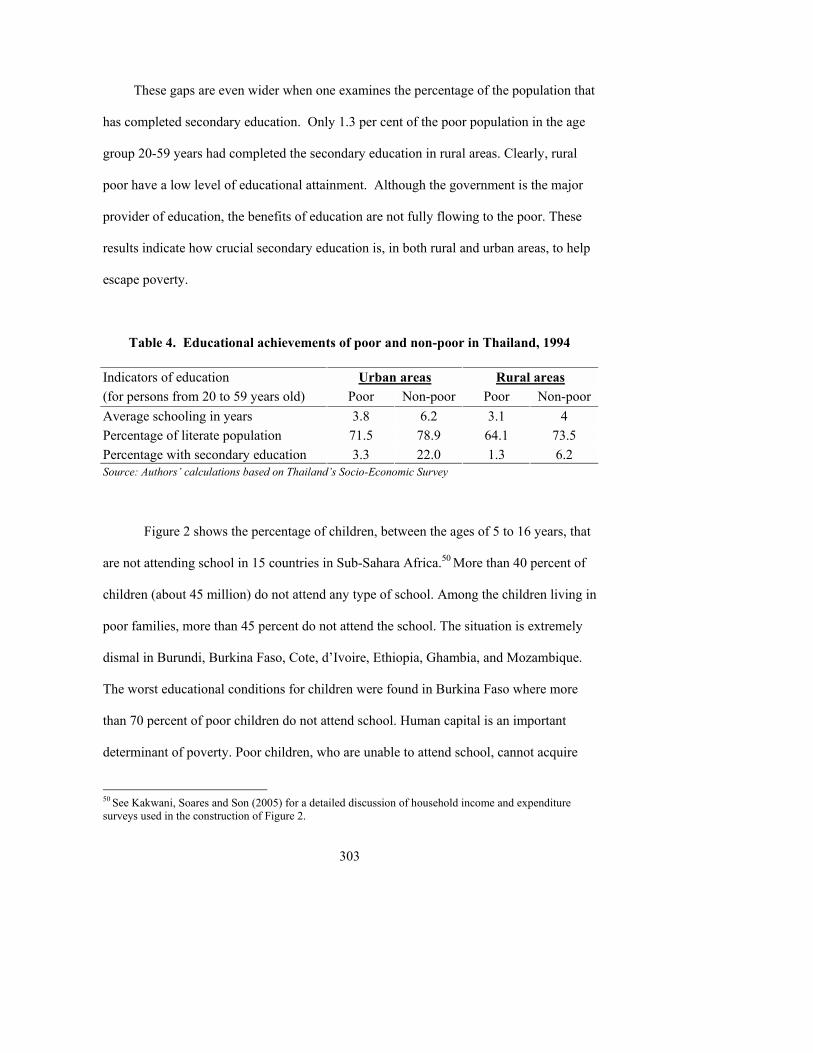
303
These gaps are even wider when one examines the percentage of the population that
has completed secondary education. Only 1.3 per cent of the poor population in the age
group 20-59 years had completed the secondary education in rural areas. Clearly, rural
poor have a low level of educational attainment. Although the government is the major
provider of education, the benefits of education are not fully flowing to the poor. These
results indicate how crucial secondary education is, in both rural and urban areas, to help
escape poverty.
Table 4. Educational achievements of poor and non-poor in Thailand, 1994
Indicators of education Urban areas Rural areas (for persons from 20 to 59 years old) Poor Non-poor Poor Non-poor Average schooling in years 3.8 6.2 3.1 4 Percentage of literate population 71.5 78.9 64.1 73.5 Percentage with secondary education 3.3 22.0 1.3 6.2 Source: Authors� calculations based on Thailand�s Socio-Economic Survey
Figure 2 shows the percentage of children, between the ages of 5 to 16 years, that
are not attending school in 15 countries in Sub-Sahara Africa.50 More than 40 percent of
children (about 45 million) do not attend any type of school. Among the children living in
poor families, more than 45 percent do not attend the school. The situation is extremely
dismal in Burundi, Burkina Faso, Cote, d�Ivoire, Ethiopia, Ghambia, and Mozambique.
The worst educational conditions for children were found in Burkina Faso where more
than 70 percent of poor children do not attend school. Human capital is an important
determinant of poverty. Poor children, who are unable to attend school, cannot acquire
50 See Kakwani, Soares and Son (2005) for a detailed discussion of household income and expenditure surveys used in the construction of Figure 2.
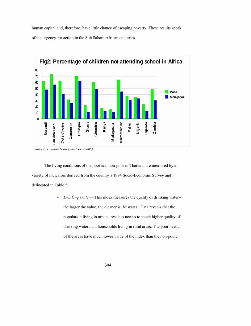
304
human capital and, therefore, have little chance of escaping poverty. These results speak
of the urgency for action in the Sub Sahara African countries.
B
urun
di
Bur
kina
Fas
o
Cot
e d'
Ivoire
Cam
eroo
n
Ethi
opia
Gha
na
Gha
mbi
a
Ken
ya
Mad
agas
car
Moz
ambi
que
Mal
awi
Nig
eria
Uga
nda
Zam
bia
0
10
2030
40
50
60
70
80
PoorNon-poor
Fig2: Percentage of children not attending school in Africa
Source: Kakwani,Soares, and Son (2005).
The living conditions of the poor and non-poor in Thailand are measured by a
variety of indicators derived from the country�s 1994 Socio-Economic Survey and
delineated in Table 5.
• Drinking Water�This index measures the quality of drinking water--
the larger the value, the cleaner is the water. Data reveals that the
population living in urban areas has access to much higher quality of
drinking water than households living in rural areas. The poor in each
of the areas have much lower value of the index than the non-poor.
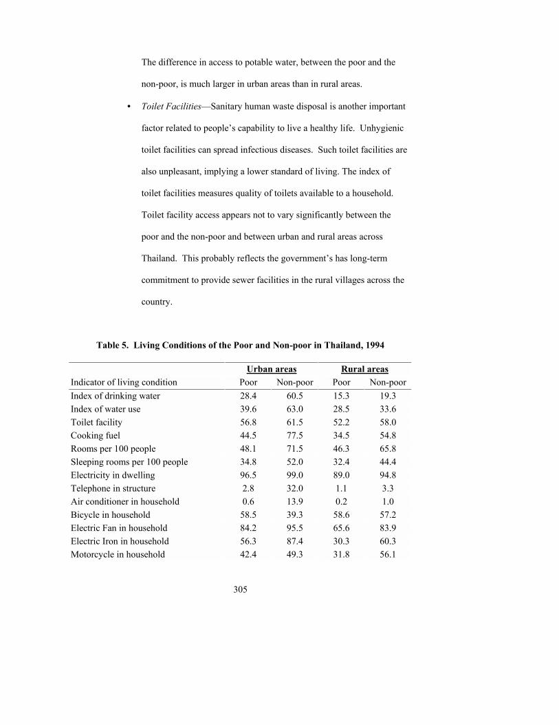
305
The difference in access to potable water, between the poor and the
non-poor, is much larger in urban areas than in rural areas.
• Toilet Facilities�Sanitary human waste disposal is another important
factor related to people�s capability to live a healthy life. Unhygienic
toilet facilities can spread infectious diseases. Such toilet facilities are
also unpleasant, implying a lower standard of living. The index of
toilet facilities measures quality of toilets available to a household.
Toilet facility access appears not to vary significantly between the
poor and the non-poor and between urban and rural areas across
Thailand. This probably reflects the government�s has long-term
commitment to provide sewer facilities in the rural villages across the
country.
Table 5. Living Conditions of the Poor and Non-poor in Thailand, 1994
Urban areas Rural areas Indicator of living condition Poor Non-poor Poor Non-poor Index of drinking water 28.4 60.5 15.3 19.3 Index of water use 39.6 63.0 28.5 33.6 Toilet facility 56.8 61.5 52.2 58.0 Cooking fuel 44.5 77.5 34.5 54.8 Rooms per 100 people 48.1 71.5 46.3 65.8 Sleeping rooms per 100 people 34.8 52.0 32.4 44.4 Electricity in dwelling 96.5 99.0 89.0 94.8 Telephone in structure 2.8 32.0 1.1 3.3 Air conditioner in household 0.6 13.9 0.2 1.0 Bicycle in household 58.5 39.3 58.6 57.2 Electric Fan in household 84.2 95.5 65.6 83.9 Electric Iron in household 56.3 87.4 30.3 60.3 Motorcycle in household 42.4 49.3 31.8 56.1
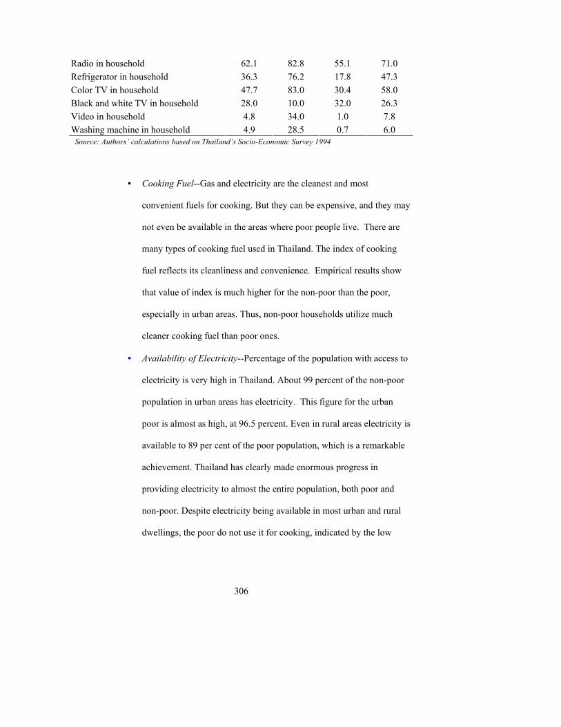
306
Radio in household 62.1 82.8 55.1 71.0 Refrigerator in household 36.3 76.2 17.8 47.3 Color TV in household 47.7 83.0 30.4 58.0 Black and white TV in household 28.0 10.0 32.0 26.3 Video in household 4.8 34.0 1.0 7.8 Washing machine in household 4.9 28.5 0.7 6.0 Source: Authors� calculations based on Thailand�s Socio-Economic Survey 1994
• Cooking Fuel--Gas and electricity are the cleanest and most
convenient fuels for cooking. But they can be expensive, and they may
not even be available in the areas where poor people live. There are
many types of cooking fuel used in Thailand. The index of cooking
fuel reflects its cleanliness and convenience. Empirical results show
that value of index is much higher for the non-poor than the poor,
especially in urban areas. Thus, non-poor households utilize much
cleaner cooking fuel than poor ones.
• Availability of Electricity--Percentage of the population with access to
electricity is very high in Thailand. About 99 percent of the non-poor
population in urban areas has electricity. This figure for the urban
poor is almost as high, at 96.5 percent. Even in rural areas electricity is
available to 89 per cent of the poor population, which is a remarkable
achievement. Thailand has clearly made enormous progress in
providing electricity to almost the entire population, both poor and
non-poor. Despite electricity being available in most urban and rural
dwellings, the poor do not use it for cooking, indicated by the low
307
index value for cooking fuel. This may be due to cost of using
electricity for cooking purposes.
• Housing Condition--SES provides data on the number of rooms (and
the number of sleeping rooms) in each dwelling. The data were used to
calculate the rooms (and sleeping room) available per 100 persons.
This index of overcrowding shows that poor people are living in more
crowded houses than non-poor people. Crowding is higher in rural
areas than in urban areas. This might be surprising because urban
areas, particularly Bangkok, seem so overcrowded.
• Access to household consumer durables--The remaining indicators in
Table 5 show a wide gap between poor and non-poor access to various
household consumer durables such as televisions, radios and videos.
Use of telephones, air conditions, and washing machines are
concentrated heavily in non-poor households located in the urban
areas. For instance, in urban areas, 32 per cent of the non-poor
population has an access to telephone, compared to only 2.8 per cent
of the poor population. In rural areas, 3.3 of non-poor have access to
phones versus 1.1 per cent of all rural poor. Similar results emerge in
the case of air conditions and washing machines. Not surprisingly,
poor households on average have more bicycles and black-and-white
televisions than non-poor households.
The above results suggest that the poor have a much lower standard of living than
the non-poor, occupying more crowded houses, with far lower access to drinking water,
308
and ownership of fewer durable goods. And the poor are less educated. It seems from
this analysis that identification of poor on the basis of income or consumption does
capture to a large extent the capability deprivation aspects of poverty. This suggests that
if policy focuses on increasing poor people�s income, it may reduce deprivation in many
other areas of capability deprivation. Alternately, governments may focus on policies and
projects that would directly deal with specific kinds of deprivation, such as the lack of
education or health. A more effective approach may be a combination of policies that
enhance people�s income and as well as reduce specific deprivations. However, from the
analysis presented here, it will be difficult to make an informed judgment about specific
policy prescriptions. More in depth policy analysis should be done.
7.1.2 Productive assets held by poor and non-poor
One of the important reasons why poverty persists is that the poor do not possess
productive assets. And the productivity of the assets they do own may be low. This is
evident from Tables 6 and 7, which review asset holdings and productivity of poor and
non-poor households in China. In rural China in 1996, the per capita value of productive
assets of poor households is 596 yuan versus 940 yuan for non-poor households. Poor
households owned 1.6 mu of arable land compared to 2.1 mu held by the non-poor.
Further, average grain production per mu was 165 for the poor households compared to
347 for non-poor households.
Table 7 shows large differences in asset holdings between the poor and non-poor
households in China in 1995. These empirical results suggest that asset holdings are
important determinants of household poverty status. To alleviate poverty, policies need to
enhance asset holdings of the poor and increase productivity of assets held by the poor.
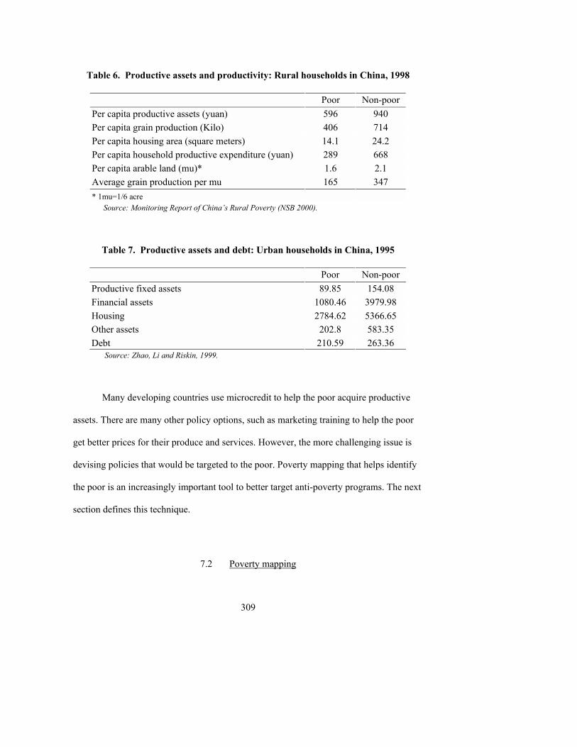
309
Table 6. Productive assets and productivity: Rural households in China, 1998
Poor Non-poor Per capita productive assets (yuan) 596 940 Per capita grain production (Kilo) 406 714 Per capita housing area (square meters) 14.1 24.2 Per capita household productive expenditure (yuan) 289 668 Per capita arable land (mu)* 1.6 2.1 Average grain production per mu 165 347 * 1mu=1/6 acre
Source: Monitoring Report of China�s Rural Poverty (NSB 2000).
Table 7. Productive assets and debt: Urban households in China, 1995
Poor Non-poor Productive fixed assets 89.85 154.08 Financial assets 1080.46 3979.98 Housing 2784.62 5366.65 Other assets 202.8 583.35 Debt 210.59 263.36
Source: Zhao, Li and Riskin, 1999.
Many developing countries use microcredit to help the poor acquire productive
assets. There are many other policy options, such as marketing training to help the poor
get better prices for their produce and services. However, the more challenging issue is
devising policies that would be targeted to the poor. Poverty mapping that helps identify
the poor is an increasingly important tool to better target anti-poverty programs. The next
section defines this technique.
7.2 Poverty mapping
310
Geographic targeting is becoming an important tool for allocating public
resources to the poor. It is increasingly regarded as a more efficient way to reduce
poverty than untargeted, universal programs. Many governments in developing countries
are giving greater importance to decentralization, whereby the district or provincial
government plays an important role in poverty reduction policies. To implement such
policies, it is important to know the spatial distribution of poverty. Poverty mapping is
the spatial analysis of poverty. It maps the incidence of poverty within each region and
sub-region of a given country. A number of methods have been devised to measure
spatial distribution of poverty. There is not enough space in this chapter to present all the
methods that have been used in practice, so only the most widely used widely method,
small-area estimation, is discussed.
Household surveys are the most important data source for measuring poverty.
However, their sample sizes are too small to provide precise estimates of poverty for
small geographical units, such as provinces and districts. An alternative data source are
population censuses, which do not suffer from small sample problems, but typically
provide very limited information from each household. For instance, censuses do not
offer information on households� consumption expenditures or incomes, preventing
income poverty from being measured directly. However, small-area estimation is a
statistical technique that combines household survey and census data to estimate income
poverty at small geographical units. It has been used by the U.S. government for planning
and targeting. And recently, the World Bank staff have refined this technique and applied
311
it to many developing countries. The technique has also been applied to Lao PDR
(Kakwani (2002), a brief discussion of which is presented below.
The first step in making a small-area estimation is to formulate a model that uses
regression methods to forecasts households� consumption expenditures, based on
household survey data. For example, let household welfare be measured by the ratio of
household consumption per capita over the per capita household poverty line (expressed
in percentage terms):
wi = 100 ci /zi (3)
where ci is the ith household�s per capita consumption and zi is the household�s per capita
poverty line. A household is poor if its welfare index in (3) is less than 100; otherwise,
it�s non-poor. Since the poverty line takes account of regional differences in costs of
living, wi is an index of household�s real per capita consumption.51 Each household i can
be characterized by the row vector of Xi, which consists of k observable household
characteristics, such as the age, sex, occupation and educational attainment of household
head, household size, location of household, access to utilities, and ownership of
consumer durables. Assume the welfare wi of household i is generated by a stochastic
model, defined as:
Ln (wi) = Xiβ + iε , (4) 51 Note that poverty lines differ across households because of differences in regional costs of living. Thus, this model attempts to explain variations in real per capita consumption that takes account of differences in regional costs of living.
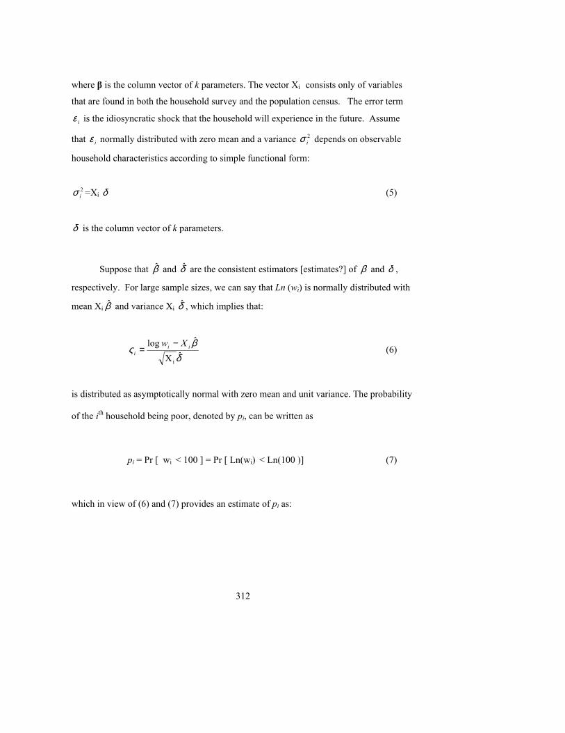
312
where β is the column vector of k parameters. The vector Xi consists only of variables
that are found in both the household survey and the population census. The error term
iε is the idiosyncratic shock that the household will experience in the future. Assume
that iε normally distributed with zero mean and a variance 2iσ depends on observable
household characteristics according to simple functional form:
2iσ =Xi δ (5)
δ is the column vector of k parameters.
Suppose that β� and δ� are the consistent estimators [estimates?] of β and δ ,
respectively. For large sample sizes, we can say that Ln (wi) is normally distributed with
mean Xi β� and variance Xi δ� , which implies that:
�X
�log
i δβς ii
iXw −
= (6)
is distributed as asymptotically normal with zero mean and unit variance. The probability
of the ith household being poor, denoted by pi, can be written as
pi = Pr [ wi < 100 ] = Pr [ Ln(wi) < Ln(100 )] (7)
which in view of (6) and (7) provides an estimate of pi as:
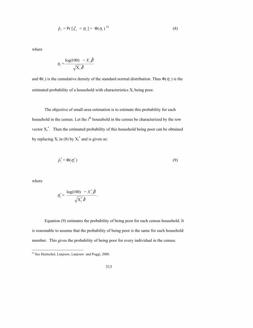
313
ip� = Pr [ iζ < iη ] = Φ( iη ) 52 (8)
where
iη = �X
�)100log(
i δ
βiX−
and Φ(.) is the cumulative density of the standard normal distribution. Thus Φ( iη ) is the
estimated probability of a household with characteristics Xi being poor.
The objective of small-area estimation is to estimate this probability for each
household in the census. Let the ith household in the census be characterized by the row
vector Xi*. Then the estimated probability of this household being poor can be obtained
by replacing Xi in (8) by Xi* and is given as:
*�� ip = Φ( *iη ) (9)
where
*iη =
�X
�)100log(*i
*
δ
βiX−.
Equation (9) estimates the probability of being poor for each census household. It
is reasonable to assume that the probability of being poor is the same for each household
member. This gives the probability of being poor for every individual in the census.
52 See Hentschel, Lanjouw, Lanjouw and Poggi, 2000.
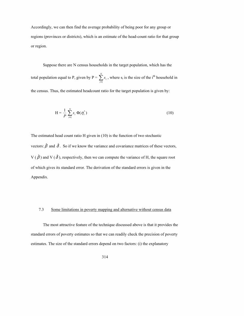
314
Accordingly, we can then find the average probability of being poor for any group or
regions (provinces or districts), which is an estimate of the head-count ratio for that group
or region.
Suppose there are N census households in the target population, which has the
total population equal to P, given by P = ∑=
N
iis
1
, where si is the size of the ith household in
the census. Thus, the estimated headcount ratio for the target population is given by:
H = P1 ∑
=
N
iis
1Φ( *
iη ) (10)
The estimated head count ratio H given in (10) is the function of two stochastic
vectors: β� and δ� . So if we know the variance and covariance matrices of these vectors,
V ( β� ) and V (δ� ), respectively, then we can compute the variance of H, the square root
of which gives its standard error. The derivation of the standard errors is given in the
Appendix.
7.3 Some limitations in poverty mapping and alternative without census data
The most attractive feature of the technique discussed above is that it provides the
standard errors of poverty estimates so that we can readily check the precision of poverty
estimates. The size of the standard errors depend on two factors: (i) the explanatory
315
power of the model estimated at the first stage from the household survey data, and (ii)
the level of disaggregation sought. Empirical analysis by Hentschel, Lanjouw, Lanjouw,
and Poggi (2000) shows that the precision of poverty estimates declines rapidly as the
degree of disaggregation increases. Thus, one cannot achieve too much fine-tuning that
might be required to achieve greater efficiency in targeting.
Household surveys generally provide information about the clusters to which the
sample households belong. This information can be exploited to obtain more efficient
estimators of the regression model. Elbers, Lanjouw, and Lanjouw (2001) have given a
detailed discussion of the econometric issues relating to the problems of
heteroskedasticity and spatial autocorrelation. These refinements will of course improve
the efficiency of estimated coefficients because they do make use of all available
information.
Construction of poverty maps requires having access to census data at the
household level. Statistical offices of many countries do not allow, for reasons of
confidentiality, such detailed information be made available to individual researchers.
Some statistical authorities, however, make available aggregated census data, which
unfortunately, leads to loss of precision of poverty map estimates, particularly at the
lower level of disaggregation. A further requirement of poverty mapping is that the
household surveys have a large subset of variables that are also in census, which may not
always be the case. Variables that are available in both household survey and census may
not be sufficiently correlated with the household consumption. In this case, the regression
316
model will not be able to predict poverty maps accurately. Finally, poverty mapping
assumes that the explanatory variables X in the household survey are produced from the
same data-generating process as the census data. This assumption, however, can be
statistically tested. The minimum requirement for this assumption to hold is that both
household and census surveys should correspond to the same period. The maximum
allowable time difference will depend on the rate of economic change that is taking place
in the country. Many countries do not have census and household surveys for the same
period.
In most developing counties, the census is conducted every ten years. Household
surveys, however, are conducted more frequently. The ten-year period is too infrequent,
leading to the creation of poverty maps that are outdated long before the next poverty
mapping exercise is undertaken. Outdated poverty maps can lead to misallocation of
scarce public resources. Given so many problems in combining household survey and
census, an alternative method of constructing partial poverty maps is proposed below.
This approach does not require the use of census data. The approach has been applied to
identify the poor districts in the Lao PDR.
Box 1: Partial Poverty Mapping in Lao PDR
There are 18 provinces in Lao PDR, each of which has many districts. The sample size can be very small at the district level, and thus the poverty estimates at the district level may not be very accurate. For the purpose of formulating a poverty reduction policy, one wants to know which districts are poor so that policymakers can target policies to them. The first task is to define a poor district. Since the poverty rate at the national level was 38.6 percent in 1997-98, it is reasonable to assume a district to be poor if more than 50 percent of its population is living in poverty. The null hypothesis is that the percentage of poor people in a district is 50 percent or less. The alternative hypothesis will obviously involve districts where more than 50 percent of the
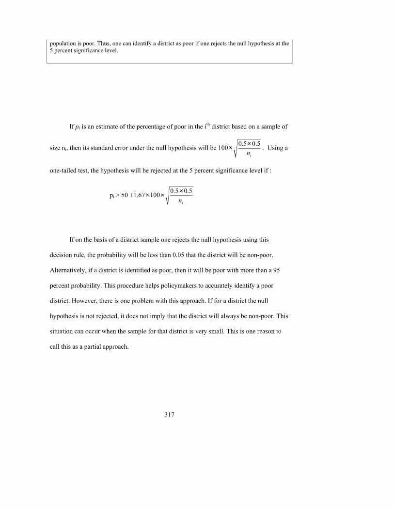
317
population is poor. Thus, one can identify a district as poor if one rejects the null hypothesis at the 5 percent significance level.
If pi is an estimate of the percentage of poor in the ith district based on a sample of
size ni, then its standard error under the null hypothesis will be 100in
5.05.0 ×× . Using a
one-tailed test, the hypothesis will be rejected at the 5 percent significance level if :
pi > 50 +1.67×100in
5.05.0 ××
If on the basis of a district sample one rejects the null hypothesis using this
decision rule, the probability will be less than 0.05 that the district will be non-poor.
Alternatively, if a district is identified as poor, then it will be poor with more than a 95
percent probability. This procedure helps policymakers to accurately identify a poor
district. However, there is one problem with this approach. If for a district the null
hypothesis is not rejected, it does not imply that the district will always be non-poor. This
situation can occur when the sample for that district is very small. This is one reason to
call this as a partial approach.
318
Empirical estimates show that of 18 provinces, the null hypothesis was rejected
for 3 provinces and 128 districts; the hypothesis of being non-poor was rejected for 28
districts. Thus this partial approach found that there are 28 districts for which over 50
percent of the population is poor. The main drawback of the approach is that one cannot
conclude how many districts are poor or non-poor in the remaining 100 districts.
7.4 Practical issues of implementing geographical targeting
Geographical targeting can be an effective means of channeling public resources
to the poor if there is a large concentration of poverty by regions. The basic idea of
geographical targeting is that the government runs the program only in the poorest
regions. If the incidence of poverty is distributed uniformly across the regions,
geographical targeting will not be very effective in reducing the national poverty. There
will be a large reduction in poverty in the targeted regions. In untargeted regions, a large
proportion of the poor will be completely left out. Thus, there will be large under-
coverage rates.
The Philippines is one of the most diverse countries in the world, making it a
revealing test of geographical targeting�s efficacy. The country can be divided into 16
regions. The second and third columns in Table 8 provide the population shares and
poverty rates in each region. The largest region is the National Capital Region (NCR)
with a population share of 14.21 percent. This is also the country�s least poor region, with
only 11.32 percent of its population considered poor. In contrast, Bicol, Caraga, and
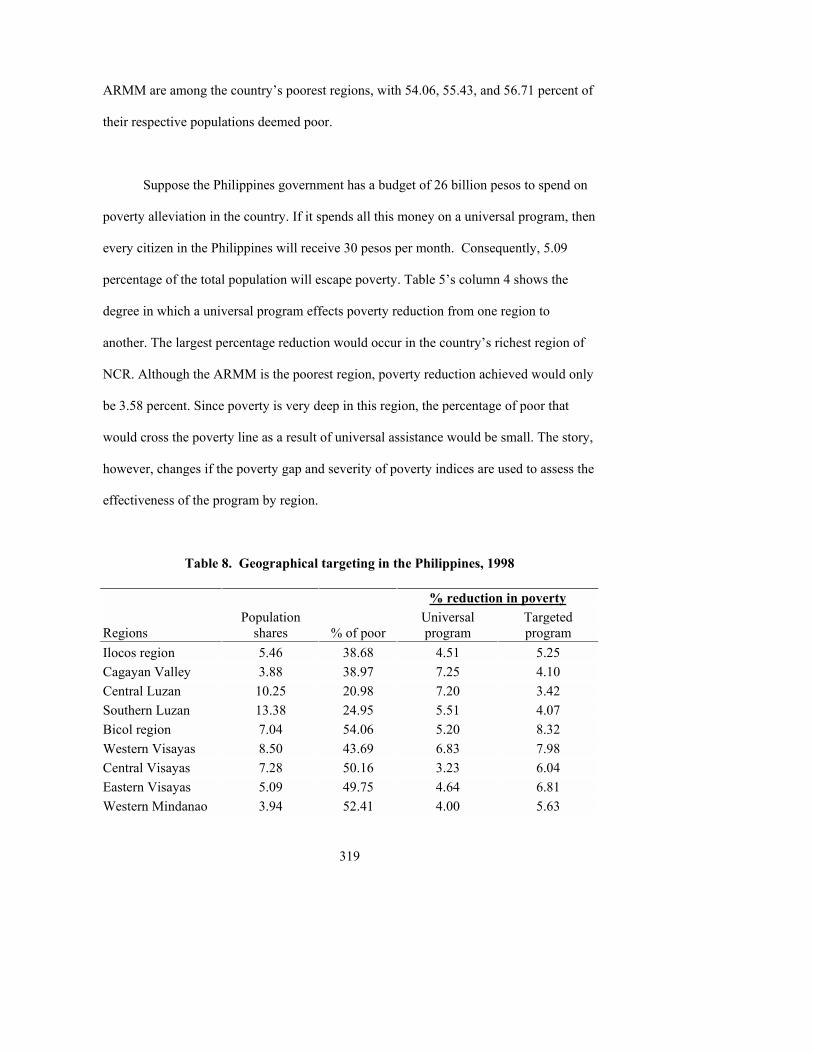
319
ARMM are among the country�s poorest regions, with 54.06, 55.43, and 56.71 percent of
their respective populations deemed poor.
Suppose the Philippines government has a budget of 26 billion pesos to spend on
poverty alleviation in the country. If it spends all this money on a universal program, then
every citizen in the Philippines will receive 30 pesos per month. Consequently, 5.09
percentage of the total population will escape poverty. Table 5�s column 4 shows the
degree in which a universal program effects poverty reduction from one region to
another. The largest percentage reduction would occur in the country�s richest region of
NCR. Although the ARMM is the poorest region, poverty reduction achieved would only
be 3.58 percent. Since poverty is very deep in this region, the percentage of poor that
would cross the poverty line as a result of universal assistance would be small. The story,
however, changes if the poverty gap and severity of poverty indices are used to assess the
effectiveness of the program by region.
Table 8. Geographical targeting in the Philippines, 1998
% reduction in poverty
Regions Population
shares % of poor Universal program
Targeted program
Ilocos region 5.46 38.68 4.51 5.25 Cagayan Valley 3.88 38.97 7.25 4.10 Central Luzan 10.25 20.98 7.20 3.42 Southern Luzan 13.38 24.95 5.51 4.07 Bicol region 7.04 54.06 5.20 8.32 Western Visayas 8.50 43.69 6.83 7.98 Central Visayas 7.28 50.16 3.23 6.04 Eastern Visayas 5.09 49.75 4.64 6.81 Western Mindanao 3.94 52.41 4.00 5.63
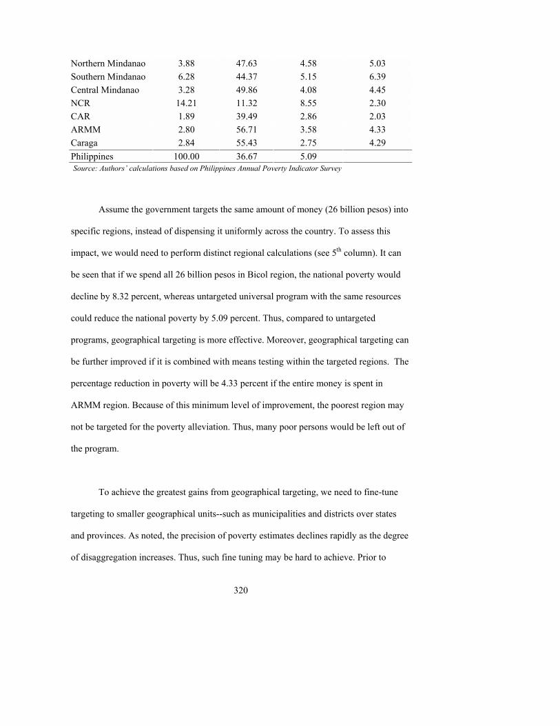
320
Northern Mindanao 3.88 47.63 4.58 5.03 Southern Mindanao 6.28 44.37 5.15 6.39 Central Mindanao 3.28 49.86 4.08 4.45 NCR 14.21 11.32 8.55 2.30 CAR 1.89 39.49 2.86 2.03 ARMM 2.80 56.71 3.58 4.33 Caraga 2.84 55.43 2.75 4.29 Philippines 100.00 36.67 5.09 Source: Authors� calculations based on Philippines Annual Poverty Indicator Survey
Assume the government targets the same amount of money (26 billion pesos) into
specific regions, instead of dispensing it uniformly across the country. To assess this
impact, we would need to perform distinct regional calculations (see 5th column). It can
be seen that if we spend all 26 billion pesos in Bicol region, the national poverty would
decline by 8.32 percent, whereas untargeted universal program with the same resources
could reduce the national poverty by 5.09 percent. Thus, compared to untargeted
programs, geographical targeting is more effective. Moreover, geographical targeting can
be further improved if it is combined with means testing within the targeted regions. The
percentage reduction in poverty will be 4.33 percent if the entire money is spent in
ARMM region. Because of this minimum level of improvement, the poorest region may
not be targeted for the poverty alleviation. Thus, many poor persons would be left out of
the program.
To achieve the greatest gains from geographical targeting, we need to fine-tune
targeting to smaller geographical units--such as municipalities and districts over states
and provinces. As noted, the precision of poverty estimates declines rapidly as the degree
of disaggregation increases. Thus, such fine tuning may be hard to achieve. Prior to
321
targeting a region, policy makers also need to have a clear idea about which poverty
measure they are attempting to reduce. It is obvious that targeted regions should deliver a
maximum reduction in national poverty. If the poverty gap is used as a poverty measure
instead of the headcount ratio, the region or regions that would be selected would be
different. The principle of horizontal equity requires that those gauged to be poor should
receive the same benefits from the government programs. Geographical targeting requires
that only those regions that can generate the largest reduction in national poverty should
be selected. This means that the poor persons in regions not selected will not receive any
benefits from the government programs.
To satisfy the principle of horizontal equity, one should use perfect targeting
when the poor get all the benefits in proportion to the income shortfall from the poverty
line (Kakwani and Son 2005). However, in practice, it is not possible to attain perfect
targeting because it is difficult to accurately determine people�s income or consumption.
Accordingly, we generally resort to proxy targeting, such as by geographical regions or
other socioeconomic characteristics of households. This leads to a violation of horizontal
equity. Thus, there is a clear-cut need for further research on targeting so that there is a
minimum violation of the principle of horizontal equity.
322
References Dollar, David ant Art Kraay (2001), � Trade, Growth and Poverty� www.Worldbank.org/research/growth/pdfiles/Trade5.pdf Deaton, A. (1997), The Analysis of Household Surveys, Baltimore and London : John Hopkins University Press Elbers, C., Lanjouw, J.O., and Lanjouw, P. (2001) �Micro-Level Estimation of Welfare,� Policy Research Working Paper No. 2911, World Bank, Washington D.C. Foster, J.E., Greer, J. and Thorbecke, E. (1984) �A Class of Decomposable Poverty Measures�, Econometrica, 52, 761-776. Hentschel, J., Lanjouw, J.O., Lanjouw, P. and Poggi, J. (2000) �Combining Census and Survey Data to Study Spatial Dimensions of Poverty: A Case Study of Ecuador,� The World Bank Economic Review. Vol. 14, No. 1, pp. 147-66. Kakwani, N. (1980), �A Class of Poverty Measures�, Econometrica, Vol. 48 Kakwani, N. (2002), �Poverty Mapping: A Case Study of Lao PDR�, unpublished mimeo, Asian Development Bank, Manila. Kakwani, N and M. Krongkaew (2000), �Analyzing Poverty in Thailand�, Journal of Asia Pacific, Vol 5, No ½, pp 140-159 Kakwani, N., Fabio, S., and Son, Hyun, H. (2005), �Conditional Cash Transfers in African Countries�, Unpublished mimeo, International Poverty Centre, Brazil. Kakwani, Nanak, and Hyun H. Son (2005). �On Assessing Pro-Poorness of Government Programmes: International Comparisons�. Working paper No. 8, International Poverty Centre, UNDP, Brasilia. Sen, A.K (1976), �Poverty: An Ordinal Approach to Measurement� Econometrica Vol. 44 Sen, A. K (1985), Commodities and Capabilities, Amsterdam: North-Holland Pyatt, G. (2000), "Poverty versus the Poor", in Rethinking Poverty: Comparative perspectives from below (ed. W. Pansters, G. Dijkstra, P. Hoebink, and E. Snel), Van Gorcum: the Netherlands. Zhao, C., Li, S., and Riskin, Z. (1999), A Restudy of Income Distribution of Chinese Residents, China Financial Economic Press.
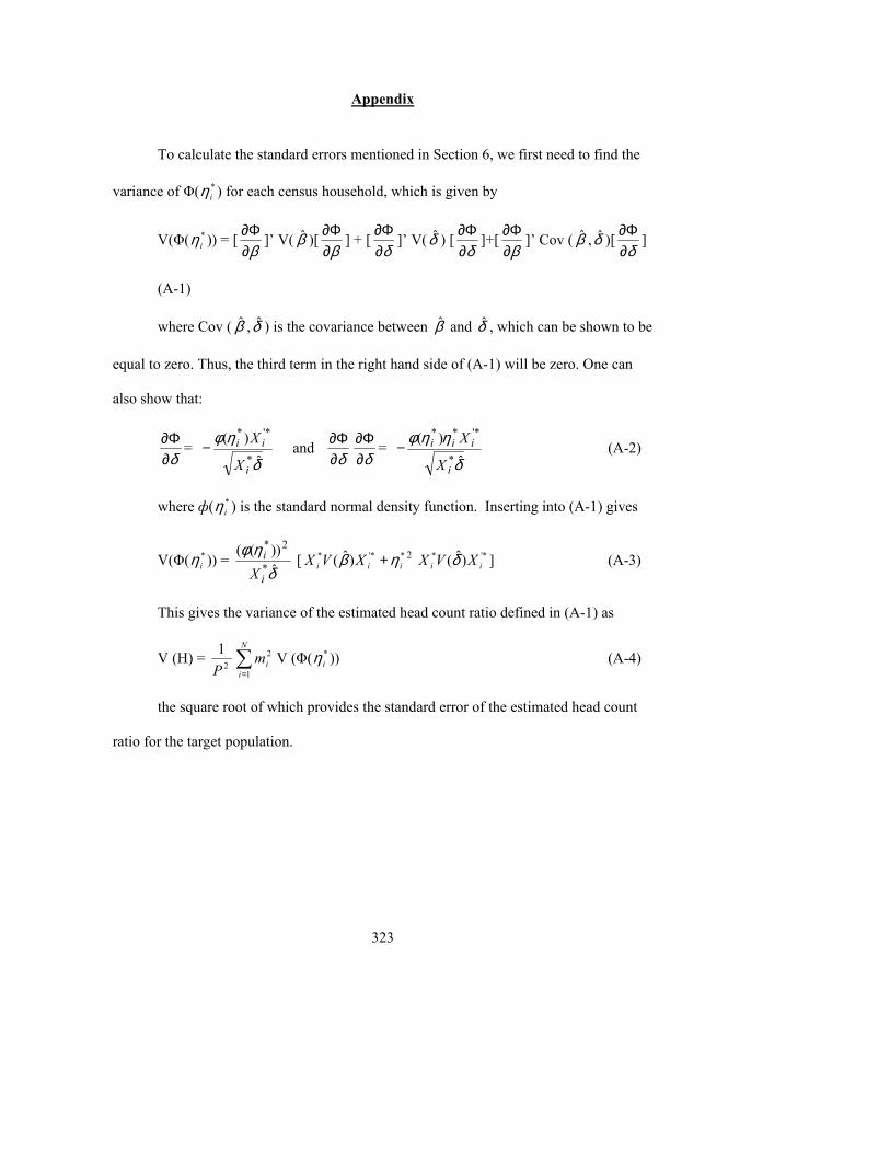
323
Appendix
To calculate the standard errors mentioned in Section 6, we first need to find the
variance of Φ( *iη ) for each census household, which is given by
V(Φ( *iη )) = [
β∂Φ∂ ]� V( β� )[
β∂Φ∂ ] + [
δ∂Φ∂ ]� V(δ� ) [
δ∂Φ∂ ]+[
β∂Φ∂ ]� Cov ( β� ,δ� )[
δ∂Φ∂ ]
(A-1)
where Cov ( β� ,δ� ) is the covariance between β� and δ� , which can be shown to be
equal to zero. Thus, the third term in the right hand side of (A-1) will be zero. One can
also show that:
δ∂Φ∂ =
δ
ηφ�
)(*
'**
i
ii
X
X− and
δ∂Φ∂
δ∂Φ∂ =
δ
ηηφ�
)(*
'***
i
iii
X
X− (A-2)
where ф( *iη ) is the standard normal density function. Inserting into (A-1) gives
V(Φ( *iη )) =
δηφ
�))((
*
2*
i
i
X [ *'** )�( iii XVX ηβ + 2 '** )�( ii XVX δ ] (A-3)
This gives the variance of the estimated head count ratio defined in (A-1) as
V (H) = 2
1P ∑
=
N
iim
1
2 V (Φ( *iη )) (A-4)
the square root of which provides the standard error of the estimated head count
ratio for the target population.
324
CHAPTER VIII. ANALYSIS OF POVERTY DYNAMICS
Paul Glewwe and John Gibson
Introduction
Chapter 7 focused almost exclusively on analysis of poverty at a single point in
time. Yet, in a given time period, people may be poor either because they�ve always
been poor or because they have suffered a negative shock that temporarily pushed them
below the poverty line. With a single cross-sectional survey, it is difficult to separate
these two types of poverty even though each may require different policy prescriptions.
Therefore, this chapter extends the analysis of Chapter 7 to many time periods, and thus
it, it is concerned with the dynamics of poverty.
Examining changes in poverty over time raises difficult issues. But it also
provides a richer and more realistic portrait of the nature of poverty. Individuals and
households typically live for many decades, which implies that a person�s poverty status
may change over time. If it does not change over time, it would be trivial to extend static
analysis to dynamic settings. As will be seen below, the poverty status of many
individuals and households appears to change a great deal over time, a finding that is
surprising to both researchers and policymakers.
This chapter assumes that �income� is an effective variable for measuring
welfare. While this assumption may narrow the scope of poverty analysis, it is needed to
325
keep the size of this chapter manageable. Even with a single�variable study, many
important issues can arise in dynamic analysis that are not simple to resolve. Thus,
despite the increased interest in poverty dynamics53 collecting and analyzing survey data
on poverty dynamics is a difficult task for any statistical agency. The chapter starts by
examining three important conceptual issues in poverty analysis in Section 8.1:
• Relationship between income inequality and poverty at a single point in
time and income mobility over time,
• Distinction between chronic and transient poverty, and
• Issues concerning the measurement of income growth among the poor.
Section 8.2 then examines two key practical issues: the relative merits of panel data
and repeated cross-sectional data, and the problem of measurement error in income and
expenditure data. Examples of how to analyze poverty dynamics are then presented in
Section 8.3. Section 8.4 concludes the chapter by summarizing its findings and
proposing several recommendations that would improve the analysis of poverty
dynamics.
8.1 Conceptual issues
The possibility that people�s poverty status can change over time raises several
conceptual issues. This section discusses three of the most important:
53 For examples, see Journal of Development Studies, August 2000 and World Development, March 2003,
326
• Understanding the relationship between income inequality and income
mobility at a single point in time (which has direct implications for the
relationship between income mobility and the dynamics of poverty),
• Distinguishing between chronic (long-run) and transient (short-run)
poverty, and
• Measuring income growth of the poor.
8.1.1 Relationship between inequality and mobility Assuming that income, or some other measurable variable, is a reasonably good
indicator of welfare, poverty can be defined by a person�s income relative to some
poverty line. One�s income determines one�s poverty status, and changes in one�s
income effects changes in one�s poverty status. Therefore, it is useful to begin by
examining the distribution of income, and changes in the distribution of income before
discussing poverty and changes in poverty.
First consider the relationship between income inequality at a single point in time
and income mobility over time. For simplicity, consider a scenario with only two time
periods. Let y1 and y2 be income in time periods 1 and 2, respectively. If people�s
incomes were unchanged in both time periods, then the distribution of y1 would be the
same as the distribution of y2. The extent of poverty (measured by comparing the
distribution of income to some poverty line) would be unchanged over time (and the
poverty status of all individuals would be the same in both time periods). But the
converse does not hold; the finding that the distribution of income has not changed over
327
time, and thus that the extent of poverty is the same in both time periods, does not imply
that everyone�s income (and poverty status) is unchanged. It is also possible that some
people who were poor in the first period escaped from poverty in the second period,
while an equal number of people who were not poor in the first time period fell into
poverty in the second period.
If it were the case that everyone�s incomes had remained unchanged over time,
then the correlation coefficient between y1 and y2 would equal one: ρ(y1, y2) = 1. On the
other hand, if some people�s incomes had increased between the two time periods so that
they escaped poverty, and they were replaced by an equal number of people who fell into
poverty over time, then the correlation between y1 and y2 would be less than one: ρ(y1, y2)
< 1. Another way of expressing this phenomenon is to say that there is a certain amount of
income mobility. Indeed, a common measure of income mobility, which can be denoted
by m(y1, y2), is one minus the correlation coefficient:
m(y1, y2) = 1 � ρ(y1, y2) (1)
where ρ(ln(y), ln(x)) is the correlation coefficient. For a more detailed exposition on
mobility, see Glewwe (2005).
In general, for a given level of short-run inequality (inequality measured at one
point in time), higher mobility implies a more equal distribution of long-run or �life
cycle� income. For example, one commonly used measure of income inequality is the
328
variance of the (natural) logarithm of income: Var[ln(y)]. In the simplest case, with only
two time periods, long-run income can be calculated as the sum of income in the two
time periods: y1 + y2. A common measure of income mobility across two time periods is
based on the correlation of the log of income:
(y1, y2) = 1 � ρ(ln(y1), ln(y2))54 (1a)
If the degree of inequality in the two time periods is similar, then long-run income
inequality is approximately equal to short-run inequality multiplied by one minus the
mobility index:
Var[ln(y1+y2)] ≈ Var[ln(y1)](1 � m(y1, y2)) (2)
where m(y1, y2) is defined as 1 � ρ(ln(y1), ln(y2)). In other words, higher income
mobility leads to lower long-run inequality for a given level of short-run inequality.
8.1.2 Chronic vs. transient poverty If poverty is defined as having an income below some poverty line in any given
year, greater mobility reduces the chance that a person who is poor in one time period is
poor in another time period (for a given rate of poverty). In fact, if the logarithm of
income (or any other monotonic transformation of income) is normally distributed in both
years, the probability that a person is poor in both years decreases as the correlation 54 In practice, it usually makes little difference whether mobility is defined as 1 � ρ(y1, y2) or 1 � ρ(ln(y1), ln(y2)). Both of these mobility indices satisfy virtually all axioms that a reasonable measure of mobility should have (see, Glewwe, 2005).
329
coefficient of y1 and y2 decreases. Put another way, greater income or expenditure
mobility implies that poverty is more of a temporary than a permanent phenomenon, and
thus that poverty is more equally distributed across the population over an individual�s
lifetimes.
The degree of income mobility, and thus the difference between short-run and
long-run inequality and the nature of poverty dynamics, is an empirical question. With
adequate data, one can measure income mobility and its consequences for long-run
inequality and the dynamics of poverty. Yet, this immediately leads to the question: How
should one measure long-run poverty at both the individual and the aggregate level? In
practice, two approaches are used to measure long-run poverty and to decompose poverty
at one point in time into a long-run, chronic component, and a short-run transient
component.
The first approach is the Spells approach, which focuses on the number of spells
of poverty experienced over a given number of time periods. This approach classifies as
chronically poor all those whose welfare is below the poverty line in all time periods. At
any point in time, the poor can be divided into the chronically poor and the transient poor,
the latter of which are poor at that time period but are not poor in one or more of the other
time periods. For multiple time periods, one can calculate the population that is
chronically poor (�always poor�) and the average population that is transient poor. The
chronically poor divided by the sum of the chronically poor and the average of the
transient poor can be used to indicate the relative contribution of chronic poverty to
330
overall poverty. The Spells approach tends to find that transient poverty is much more
common than chronic poverty. In a review of 13 studies, 11 found that the chronically
poor were a smaller proportion of the overall population than the transient poor (Baulch
and Hoddinott, 2000).
There are several disadvantages of using the Spells approach to divide overall poverty
into chronic and transient poverty. First, it is sensitive to measurement error, which leads
to overestimation of the proportion of the population that is poor in some time periods but
not in others. Second, it focuses attention on the headcount measure of poverty. In
contrast, the poverty gap and distributionally-sensitive poverty measures (see Chapter 7)
may record greater amounts of chronic poverty (as a proportion of overall poverty)
because at a single point in time the chronic poor are most likely to be further below the
poverty line. Third, the results are very likely to be sensitive to how many survey waves
are available. It is harder for a household to be recorded as always poor in ten successive
surveys than in just two of them. Similarly, when there are, say, ten survey waves,
�sometimes poor� includes those who are poor once in ten periods and those who are
poor in nine times out of ten, which is probably too broad a group to be meaningful. For
example, across eight waves of data in the Russian Longitudinal Monitoring Survey
(RLMS), gathered between 1994 and 2003, only four percent of urban households were
always poor, while 81 percent were sometimes poor. But if only two waves of data are
used (averaging over all possible combinations), 19 percent appear to be always poor and
36 percent appear to be sometimes poor. The ratio of always-to-sometimes poor, which
331
can indicate chronic poverty, is thus not easily compared across surveys where
households are observed across a different number of time periods.
An alternative method to the Spells approach is to divide poverty into the
permanent component of a household�s income (or consumption expenditures) and the
remaining poverty due to transitory changes in income (Jalan and Ravallion, 1998).
Under this Components approach, the chronically poor are those whose mean welfare
across time is below the poverty line. The extent of chronic poverty is a function of that
household�s mean income, ( , , , )i i i iC P y y y= K , where iy is the mean welfare for
household i over the T time periods spanned by the survey, and P is a poverty measure,
such as the headcount or poverty gap. Transient poverty is the remainder, when Ci is
subtracted from the total poverty measure at each point in time:
1 2( , , , ) ( , , , ).i i i iK i i iT P y y y P y y y= −K K
A simple example can help distinguish between the Spells and Components approaches.
Consider four individuals, whose two-period consumption vectors are: A={450, 450},
B={400, 550}, C={530, 460}, and D={600, 550}. The poverty line is set at 500 in both
periods. It is clear that person A is always poor, while B and C are sometimes poor, and
D is never poor. Using the Spells approach to measure chronic poverty, one might
conclude that the chronic poverty share of total poverty is one-third. However, persons A,
B, and C are all chronically poor under the Components approach because their average
consumption over time is below the poverty line.
332
The Components approach measures poverty in each period, using the period-
specific consumption, and subtracts from this the poverty measure at the person�s average
consumption. For example, using the poverty gap index, the total poverty measures are:
• [((500-450)/500)+ ((500-450)/500)]/2=0.10, for person A
• [((500-400)/500)+ 0]/2=0.10, for person B, and
• [0+ ((500-460)/500)]/2=0.04, for person C.
The chronic poverty measures are:
• (500-450)/500)=0.10, for person A
• (500-475)/500)=0.05, for person B, and
• (500-495)/500)=0.01, for person C.
Therefore, the transient components are 0, 0.05 and 0.03, respectively. Aggregating over
the whole population of three people, the total poverty gap index is 0.06, the chronic
poverty index is 0.04, and the transient poverty index is 0.02. In contrast to the Spells
approach, two-thirds of the poverty appears to be chronic and only one-third transient.
This example highlights the impact various methodological approaches have on
conclusions drawn about chronic and transient poverty. A further example comes from
the RLMS data referred to above. According to the Components approach, chronic
poverty makes up 57 percent of the total amount of poverty, and it is only during Wave 8
(in 1998 during the Russian financial crisis) that the contribution from transient poverty
exceeds that from chronic poverty (Figure 1).
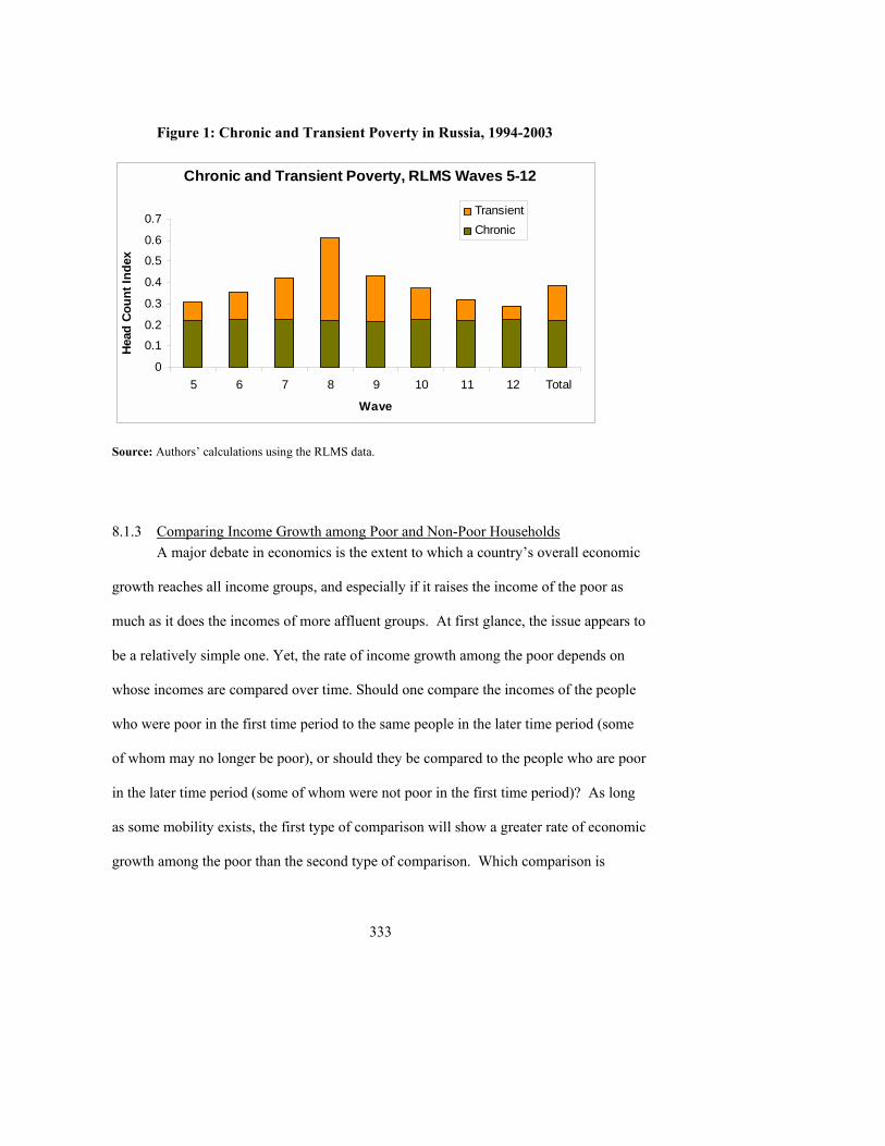
333
Figure 1: Chronic and Transient Poverty in Russia, 1994-2003
Chronic and Transient Poverty, RLMS Waves 5-12
0
0.1
0.2
0.3
0.4
0.5
0.6
0.7
5 6 7 8 9 10 11 12 Total
Wave
Hea
d C
ount
Inde
x
TransientChronic
Source: Authors� calculations using the RLMS data.
8.1.3 Comparing Income Growth among Poor and Non-Poor Households A major debate in economics is the extent to which a country�s overall economic
growth reaches all income groups, and especially if it raises the income of the poor as
much as it does the incomes of more affluent groups. At first glance, the issue appears to
be a relatively simple one. Yet, the rate of income growth among the poor depends on
whose incomes are compared over time. Should one compare the incomes of the people
who were poor in the first time period to the same people in the later time period (some
of whom may no longer be poor), or should they be compared to the people who are poor
in the later time period (some of whom were not poor in the first time period)? As long
as some mobility exists, the first type of comparison will show a greater rate of economic
growth among the poor than the second type of comparison. Which comparison is
334
correct? Both are informative, and both need to be considered when asking whether
economic growth has been �pro-poor.�
8.2 Data issues
All the issues discussed in the previous section assume that once the conceptual
issues are settled, data will be available to measure poverty and changes in poverty in
accordance with the concepts deemed to be most correct. Yet, data from both developed
and developing countries often fall short of the needs of researchers and policymakers
who are interested in poverty issues. This section focuses on two important issues: the
strengths and weaknesses of panel data and repeated cross-sectional data, and the
problem of measurement error in the data.
8.2.1 Panel Data versus Repeated Cross-Sectional Data Poverty dynamics is almost always measured by examining household survey
data collected at two or more time periods. A very important characteristic of a
household survey is whether the data are collected from the same households and
individuals over time (called panel data) or if the data are collected from different
households each time the survey is conducted (known as a repeated cross-sectional
survey). In general, panel data provide much more information on poverty dynamics
than do repeated cross-sectional data. But panel data are somewhat more complicated to
collect.
335
To see the benefit of panel data, first consider the persistence of poverty over
time, which, as explained above, is closely related to income mobility. Neither income
mobility nor persistence of poverty can be measured using repeated cross-sectional data.
Only panel data track the same people and households over time and thus reveal the
extent to which people�s incomes change over time, and the extent to which poverty is
either permanent or temporary. Thus, panel data are required to separate overall poverty
into its chronic and transient components. Second, consider the impact of economic
growth on the poor. Both cross-sectional and panel data can be used to measure income
growth among the poor if the poor are defined in terms of the current status (e.g., the
poorest 20 percent of the population in each year). However, only panel data allow one
to examine income growth among the poor when it is defined as following the same
people over time (and thus who may not be in the poorest 20 percent of the population in
later years). Again, the reason for this is that panel data track the same people and
households over time, while cross-sectional data collect data from different people over
time.
While panel data have the above-mentioned advantages, they also have three
potential disadvantages. First, under even the best circumstances some households and
individuals that are part of the original data are lost--they refuse to participate or cannot
be found in later interviews. This phenomenon is known as sample attrition, and if the
individuals and households that cannot be reinterviewed are systematically different from
those that remain, the latter are not a random sample of the population and thus may yield
biased estimates. Second, as new people are born and new households are formed, there
336
is often a tendency to exclude them from the sample because those people and
households did not exist when the sample was originally collected. While this potential
source of bias, known as selection bias, can be overcome in principal by following
households that �split off� from the original households in the survey, doing so is
difficult and in practice is often not done. The third disadvantage of collecting data is
that it may be somewhat more expensive to collect than implementing a series of repeated
cross-sectional surveys.
While these limitations of panel data must be taken seriously, such data still
provide much more information on poverty dynamics over time than does a series of
cross-sectional surveys that interview different households at each point in time. Because
the effect of these disadvantages can be mitigated (see Glewwe and Jacoby, 2000), this
chapter recommends that panel data be collected if one wants to analyze poverty
dynamics. This is not a simple task, but it is feasible in many developing countries.
Further analysis and recommendations for how to collect panel data can be found in
Glewwe and Jacoby (2000).
8.2.2 Measurement Error A second key issue is measurement error in the income (or expenditure) data.
Empirical studies of poverty dynamics, and more generally of income mobility, typically
use income and/or expenditure data collected from household surveys. Anyone who has
seen how such data are collected understands that these variables are likely to be
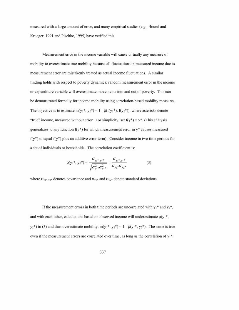
337
measured with a large amount of error, and many empirical studies (e.g., Bound and
Krueger, 1991 and Pischke, 1995) have verified this.
Measurement error in the income variable will cause virtually any measure of
mobility to overestimate true mobility because all fluctuations in measured income due to
measurement error are mistakenly treated as actual income fluctuations. A similar
finding holds with respect to poverty dynamics: random measurement error in the income
or expenditure variable will overestimate movements into and out of poverty. This can
be demonstrated formally for income mobility using correlation-based mobility measures.
The objective is to estimate m(y1*, y2*) = 1 - ρ(f(y1*), f(y2*)), where asterisks denote
�true� income, measured without error. For simplicity, set f(y*) = y*. (This analysis
generalizes to any function f(y*) for which measurement error in y* causes measured
f(y*) to equal f(y*) plus an additive error term). Consider income in two time periods for
a set of individuals or households. The correlation coefficient is:
ρ(y1*, y2*) = **
**,
2*
2*
**,
21
21
21
21
yy
yy
yy
yy
σσ
σ
σσ
σ= (3)
where σy1*,y2* denotes covariance and σy1* and σy2* denote standard deviations.
If the measurement errors in both time periods are uncorrelated with y1* and y2*,
and with each other, calculations based on observed income will underestimate ρ(y1*,
y2*) in (3) and thus overestimate mobility, m(y1*, y2*) = 1 - ρ(y1*, y2*). The same is true
even if the measurement errors are correlated over time, as long as the correlation of y1*
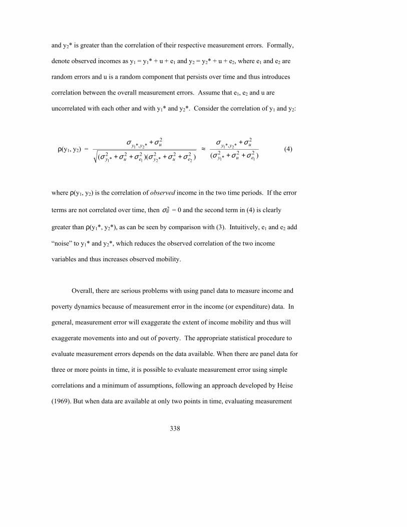
338
and y2* is greater than the correlation of their respective measurement errors. Formally,
denote observed incomes as y1 = y1* + u + e1 and y2 = y2* + u + e2, where e1 and e2 are
random errors and u is a random component that persists over time and thus introduces
correlation between the overall measurement errors. Assume that e1, e2 and u are
uncorrelated with each other and with y1* and y2*. Consider the correlation of y1 and y2:
ρ(y1, y2) = ))(( 222
*222
*
2**,
2211
21
euyeuy
uyy
σσσσσσ
σσ
++++
+ ≈
)( 222*
2**,
11
21
euy
uyy
σσσ
σσ
++
+ (4)
where ρ(y1, y2) is the correlation of observed income in the two time periods. If the error
terms are not correlated over time, then 2uσ = 0 and the second term in (4) is clearly
greater than ρ(y1*, y2*), as can be seen by comparison with (3). Intuitively, e1 and e2 add
�noise� to y1* and y2*, which reduces the observed correlation of the two income
variables and thus increases observed mobility.
Overall, there are serious problems with using panel data to measure income and
poverty dynamics because of measurement error in the income (or expenditure) data. In
general, measurement error will exaggerate the extent of income mobility and thus will
exaggerate movements into and out of poverty. The appropriate statistical procedure to
evaluate measurement errors depends on the data available. When there are panel data for
three or more points in time, it is possible to evaluate measurement error using simple
correlations and a minimum of assumptions, following an approach developed by Heise
(1969). But when data are available at only two points in time, evaluating measurement
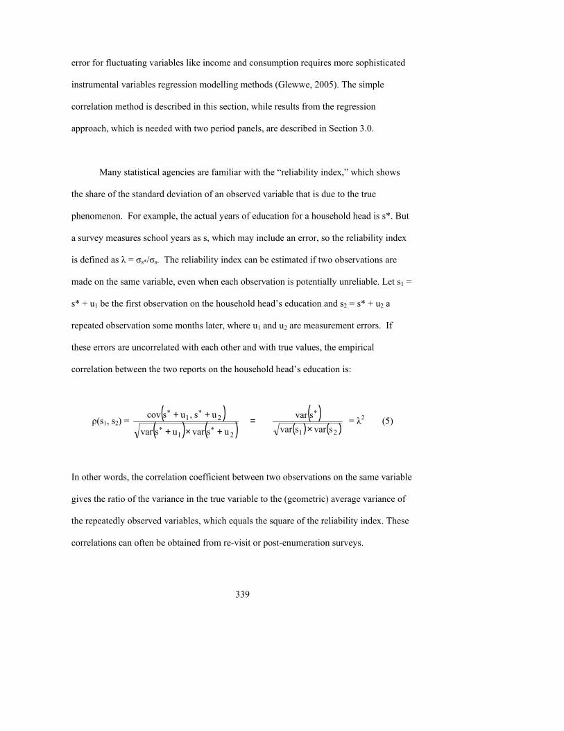
339
error for fluctuating variables like income and consumption requires more sophisticated
instrumental variables regression modelling methods (Glewwe, 2005). The simple
correlation method is described in this section, while results from the regression
approach, which is needed with two period panels, are described in Section 3.0.
Many statistical agencies are familiar with the �reliability index,� which shows
the share of the standard deviation of an observed variable that is due to the true
phenomenon. For example, the actual years of education for a household head is s*. But
a survey measures school years as s, which may include an error, so the reliability index
is defined as λ = σs*/σs. The reliability index can be estimated if two observations are
made on the same variable, even when each observation is potentially unreliable. Let s1 =
s* + u1 be the first observation on the household head�s education and s2 = s* + u2 a
repeated observation some months later, where u1 and u2 are measurement errors. If
these errors are uncorrelated with each other and with true values, the empirical
correlation between the two reports on the household head�s education is:
ρ(s1, s2) = ( )
( ) ( )( )
( ) ( )21
*
2*
1*
2*
1*
svarsvarsvar
usvarusvar
us,uscov×
=+×+
++ = λ2 (5)
In other words, the correlation coefficient between two observations on the same variable
gives the ratio of the variance in the true variable to the (geometric) average variance of
the repeatedly observed variables, which equals the square of the reliability index. These
correlations can often be obtained from re-visit or post-enumeration surveys.
340
The reliability index cannot be directly applied to longitudinal data on income or
consumption, because unlike years of education in the above example, the true values of
income and consumption fluctuate over time. Thus a correlation of less than one for the
consumption of the same household in two periods does not necessarily indicate
measurement error and instead may reflect an inability to smooth consumption over time.
However, if there are at least three waves in a longitudinal survey, it is possible to
separate real dynamics from measurement error with minimal assumptions (Heise, 1969).
Intuition suggests that the estimated correlation between a mis-measured variable, like
household consumption in one period, and a realization of that variable in a subsequent
period will be less than it would be in the absence of measurement error (as explained
above). And this attenuation is proportional to the reliability index of the variable.
As an example, consider the reliability index for household consumption in the
Russian Longitudinal Monitoring Survey. Let Y1994, Y1995, and Y1996 be the observed
consumption for the 2,195 urban households in the survey in each of 1994, 1995 and
1996. The true but unknown consumption is X1994, X1995, and X1996, which differs from
the observed values due to measurement errors that are independent of each other, of
time, and of the underlying variable: .t t tY X u t= + ∀ If the reliability of measuring
consumption does not vary over time, the correlation between observed consumption in
two years is: ρ(Yt, Yt+1) = λYtλYt+1ρ(Xt, Xt+1) = (λY)2ρ(Xt, Xt+1). So for example, the
correlation of 0.42 between observed expenditures in 1994 and 1995 understates the
correlation in actual consumption by a factor of (λY)2. These assumptions also imply that
341
ρ(Yt-1, Yt+1) = (λY)2ρ(Xt-1, Xt+1). If realizations of the true values of consumption come
from a first-order autoregressive model (that is, if Xt = a + bXt-1 + et), then the
relationship between correlation coefficients is: ρ(Xt-1, Xt)×ρ(Xt, Xt+1)/ρ(Xt-1, Xt+1) = 1.
Substituting in the results [Not clear] for the correlation in observed consumption, the
reliability index is estimated as: λY = )Y,Y(
)Y,Y()Y,Y(
1t1t
1ttt1t
+−
+−ρ
ρρ. Applying this formula to
the Russian data, λy = )Y,Y(
)Y,Y()Y,Y(
19961994
1996199519951994ρ
ρρ =
29.051.042.0 × = 0.86.
In other words, the standard deviation of observed household consumption in the Russian
data can be decomposed into a true component, which contributes 86 percent, and an
error component, which contributes 14 percent. It is because of this error, which
attenuates correlations, that the product of the two one-year apart
correlations, 0.42 0.51 ( 0.22)× = , is less than the two-year apart correlation, 0.29.
A further example of this reliability index calculation comes from the Indonesian
Family Life Survey, which observed a panel of households in 1993, 1997 and 2000. The
correlations between the logarithm of annualized expenditures in each of these three
years are reported in Table 1. It is apparent that there was a closer relationship between
expenditures in 1997 and in 2000 than between 1993 and 1997, which may reflect some
changes in the questionnaire.55 The measure of mobility for 1997-2000, 1 � ρ(ln(y1),
ln(y2)) gives values of 0.32-0.40 similar to those reported for Vietnam in Table 5 below.
However, this measure of mobility is based on attenuated correlation coefficients, where 55 Correlations between other variables, like age of the household head, which should be measured with less error, also show this pattern. Researchers should use such correlations to check that they have correctly identified panel households.
342
the attenuation is given by 2.Yλ The estimates of 2Yλ vary from 0.68-0.73 by sector and
once these are used to correct the correlations for the effect of measurement error, the
mobility measures fall substantially to only 0.06-0.12.
Table 1: Correlations Between Annualized Expenditures and Mobility of Households in Indonesia, With Correction for Measurement Error
Correlations Indonesia Urban Rural1993_2000 0.4288 0.4362 0.33221993_1997 0.4684 0.4656 0.37851997_2000 0.6717 0.6775 0.6 Reliability ratio 0.73 0.72 0.68Reliability index 0.86 0.85 0.83 Mobility index (1997-2000) 0.33 0.32 0.40Corrected correlation (1997-2000) 0.92 0.94 0.88Corrected mobility index 0.08 0.06 0.12
Source: Authors� calculations using Indonesian Family Life Survey (IFLS) data
8.3 Recommendations for Data Collection
Evidence of measurement error in the expenditure data from the Russian and
Indonesian panels, which are two of the better regarded surveys from developing
countries, illustrates the need to address this issue. Fortunately, panel data allow one to
use methods that assess and correct for measurement error, methods that cannot be used
with cross-sectional data. If statistical agencies in developing countries are interested in
measuring poverty dynamics, they will need to collect panel data. This subsection
provides some recommendations for doing so.
343
First, it is important that the sample involve households (or even more thoroughly,
of individuals) rather than dwellings. Otherwise, replacing an old household with a new
one in a sampled dwelling may create spurious evidence of changes in economic status.
More specifically, any panel sample that returns to the same dwellings over time must
collect sufficient data to ascertain whether the dwelling�s inhabitants are the same
household or a new household. (Methods for doing so are provided in Glewwe and
Jacoby, 2000.) A better approach would be for the survey to follow households that
move and those that split and re-form (e.g., following marriage and divorce) because the
poverty status of movers is often different from that of people who maintain stable
addresses and family circumstances.
Second, consideration must be given to sample attrition, which may lead to
selective samples of stayers that yield misleading inferences about the population.
Fortunately, for some purposes, sample attrition may not be a serious problem. For
example, Falaris (2003) studied attrition in several LSMS surveys. Stayers were 31
percent of the initial sample for Peru between 1991 and 1994, 55 percent for Lima
between 1985 and 1990, 82 percent for Côte d�Ivoire between 1985 and 1988, and 84
percent for Vietnam between 1993 and 1998. Despite this wide variation in attrition rates,
regression relationships for schooling attainment, wages and other socio-economic
outcomes do not seem to vary between �attritors� and stayers in these samples. Lack of
attrition bias suggests that results from just the sample of stayers are also likely to apply
344
to attritors. Similar conclusions have been reached for regression studies on longitudinal
data in developed countries (Fitzgerald, Gottschalk and Moffitt, 1998).
Yet, it is not clear whether the relatively minor affects of attrition on the
conditional mean in regression studies also holds for poverty studies, which focus on the
lower tail of the distribution. There is surprisingly little evidence on the effects of
attrition on observed poverty dynamics in developing countries. However, at least in
developed countries, it seems that attrition creates a bias. Cappellari and Jenkins (2002)
use the British Household Panel Survey and find that a sample that excludes attritors
would disproportionately exclude the poor and cause an overestimation of poverty
persistence.
One way to reduce the potential for attrition bias is for statistical agencies to
change the way in which they implement longitudinal surveys. Many surveys in
developing countries attempt to re-interview respondents only if they live in the same
dwelling in which they were previously interviewed. Failure to track movers presumably
reflects concerns about cost and feasibility. Nevertheless, the experience of the
Indonesian Family Life Survey shows that many movers can be successfully tracked,
even when they move to a new province. In that survey, households who moved locally
have initial characteristics that are more like those who stay in the same dwelling,
whereas those who move longer distances are more like attritors. So there is considerable
information gained by making the effort to track the movers (Thomas, Frankenberg and
Smith, 2001).
345
8.4 Analytical methods with examples
8.4.1 Repeated cross-sectional data (including poverty monitoring) If one has two or more cross-sectional data sets, one can use them to measure the
extent, characteristics, and distribution of poverty across population groups, and how all
of these things change over time. In addition, one can measure the average income of the
poorest 10 percent, 20 percent, or 30 percent (or any percentage that is of interest) and
see how the income of these groups changes over time. These percentile-specific
comparisons provide one way of considering how the effect of growth at different points
in income distribution might affect poverty.
An alternative method, which also requires only repeated cross-sections, is to
decompose the change in poverty between two surveys into a �distribution� component
and a �growth� component. The distribution component reflects the hypothetical effect
of changes in inequality while holding mean (real) income constant. In contrast, the
growth effect allows (real) mean to change at the rate of economic growth while
(counterfactually) holding the distribution of income (as measured by the Lorenz curve)
constant. This decomposition is of interest because the appropriate policies for reducing
poverty will depend on whether recent changes in poverty are due mainly to growth
effects or to inequality effects.
346
This subsection presents examples of all of these, mainly using household survey
data from Vietnam and Papua New Guinea. Vietnam is an interesting example because
its high rate of economic growth led to a large decline in poverty, from about 58 percent
in 1992-93 to about 37 percent in 1997-98 (World Bank, 1999). In such circumstances, it
is usually clear that the growth component of the poverty change is dominant. In
contrast, poverty in Papua New Guinea has been much more persistent (Gibson, 2000).
Therefore, to provide an example where it is less clear whether it is the growth or the
inequality component that is likely to dominate, this subsection illustrates decomposition
methods using data from urban Papua New Guinea.
Table 2 shows the extent of poverty in Vietnam in 1992-93 and 1997-98 using
two common poverty indices: the headcount index (proportion of the people who are
poor) and the poverty gap index (see Chapter 7 for an explanation).56 Figures are shown
separately for urban and rural areas, as well as for the entire country. The incidence of
poverty in Vietnam dropped from 58.1 percent in 1992-93 to 37.4 percent in 1997-98.
The drop in the poverty gap is even more dramatic, cut almost in half from 0.185 to
0.095. Using either index of poverty, it is clear that poverty dropped much more rapidly
in urban areas than in rural areas. For example, in urban areas the incidence of poverty
declined by more than half, from 25.1 percent to 9.0 percent, while in rural areas the
poverty rate dropped from 66.4 percent to 44.9 percent.
Table 2: Poverty in Vietnam in 1992-93 and 1997-98 56 For more information on the 1992-93 and 1997-98 Vietnam Living Standards Survey, see World Bank (2001).
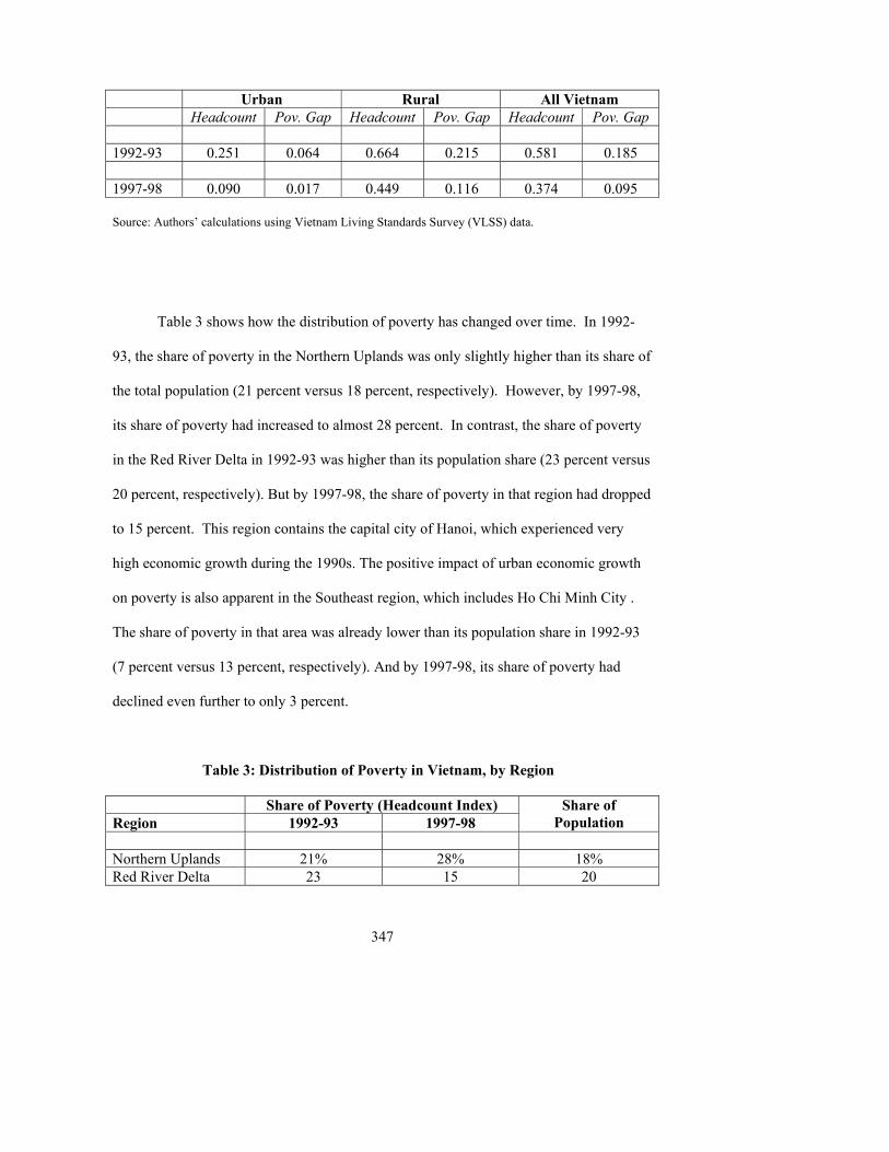
347
Urban Rural All Vietnam Headcount Pov. Gap Headcount Pov. Gap Headcount Pov. Gap 1992-93 0.251 0.064 0.664 0.215 0.581 0.185 1997-98 0.090 0.017 0.449 0.116 0.374 0.095 Source: Authors� calculations using Vietnam Living Standards Survey (VLSS) data.
Table 3 shows how the distribution of poverty has changed over time. In 1992-
93, the share of poverty in the Northern Uplands was only slightly higher than its share of
the total population (21 percent versus 18 percent, respectively). However, by 1997-98,
its share of poverty had increased to almost 28 percent. In contrast, the share of poverty
in the Red River Delta in 1992-93 was higher than its population share (23 percent versus
20 percent, respectively). But by 1997-98, the share of poverty in that region had dropped
to 15 percent. This region contains the capital city of Hanoi, which experienced very
high economic growth during the 1990s. The positive impact of urban economic growth
on poverty is also apparent in the Southeast region, which includes Ho Chi Minh City .
The share of poverty in that area was already lower than its population share in 1992-93
(7 percent versus 13 percent, respectively). And by 1997-98, its share of poverty had
declined even further to only 3 percent.
Table 3: Distribution of Poverty in Vietnam, by Region
Share of Poverty (Headcount Index) Region 1992-93 1997-98
Share of Population
Northern Uplands 21% 28% 18% Red River Delta 23 15 20
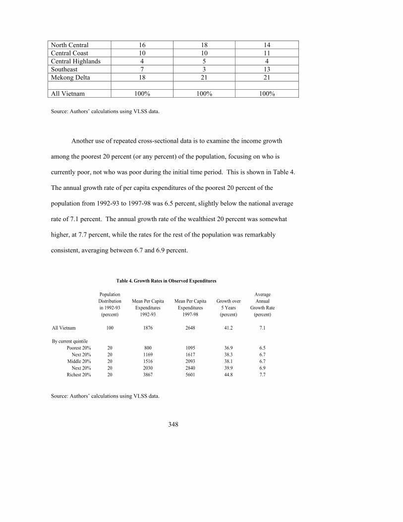
348
North Central 16 18 14 Central Coast 10 10 11 Central Highlands 4 5 4 Southeast 7 3 13 Mekong Delta 18 21 21 All Vietnam 100% 100% 100%
Source: Authors� calculations using VLSS data.
Another use of repeated cross-sectional data is to examine the income growth
among the poorest 20 percent (or any percent) of the population, focusing on who is
currently poor, not who was poor during the initial time period. This is shown in Table 4.
The annual growth rate of per capita expenditures of the poorest 20 percent of the
population from 1992-93 to 1997-98 was 6.5 percent, slightly below the national average
rate of 7.1 percent. The annual growth rate of the wealthiest 20 percent was somewhat
higher, at 7.7 percent, while the rates for the rest of the population was remarkably
consistent, averaging between 6.7 and 6.9 percent.
Table 4. Growth Rates in Observed Expenditures
Population AverageDistribution Mean Per Capita Mean Per Capita Growth over Annualin 1992-93 Expenditures Expenditures 5 Years Growth Rate(percent) 1992-93 1997-98 (percent) (percent)
All Vietnam 100 1876 2648 41.2 7.1
By current quintilePoorest 20% 20 800 1095 36.9 6.5
Next 20% 20 1169 1617 38.3 6.7Middle 20% 20 1516 2093 38.1 6.7
Next 20% 20 2030 2840 39.9 6.9Richest 20% 20 3867 5601 44.8 7.7
Source: Authors� calculations using VLSS data.
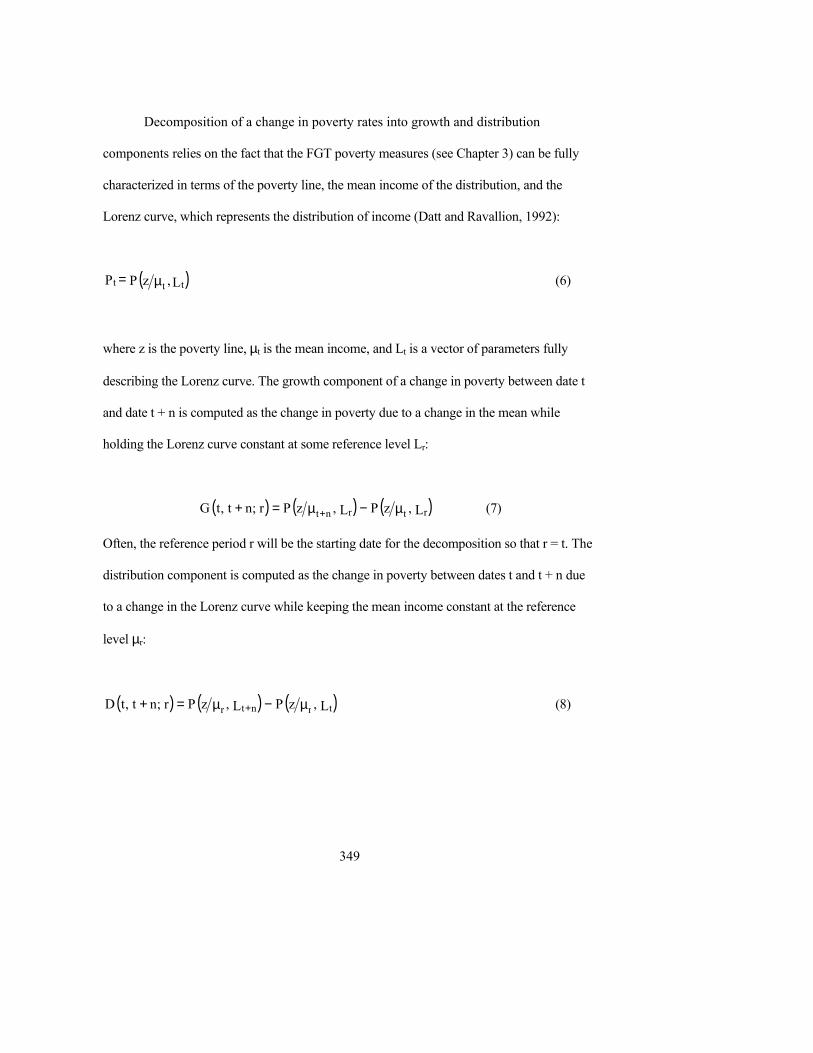
349
Decomposition of a change in poverty rates into growth and distribution
components relies on the fact that the FGT poverty measures (see Chapter 3) can be fully
characterized in terms of the poverty line, the mean income of the distribution, and the
Lorenz curve, which represents the distribution of income (Datt and Ravallion, 1992):
( )L,zPP ttt µ= (6)
where z is the poverty line, µt is the mean income, and Lt is a vector of parameters fully
describing the Lorenz curve. The growth component of a change in poverty between date t
and date t + n is computed as the change in poverty due to a change in the mean while
holding the Lorenz curve constant at some reference level Lr:
( ) ( ) ( )L,zPL,zPr;nt,tG rtrnt µ−µ=+ + (7)
Often, the reference period r will be the starting date for the decomposition so that r = t. The
distribution component is computed as the change in poverty between dates t and t + n due
to a change in the Lorenz curve while keeping the mean income constant at the reference
level µr:
( ) ( ) ( )L,zPL,zPr;nt,tD trntr µ−µ=+ + (8)
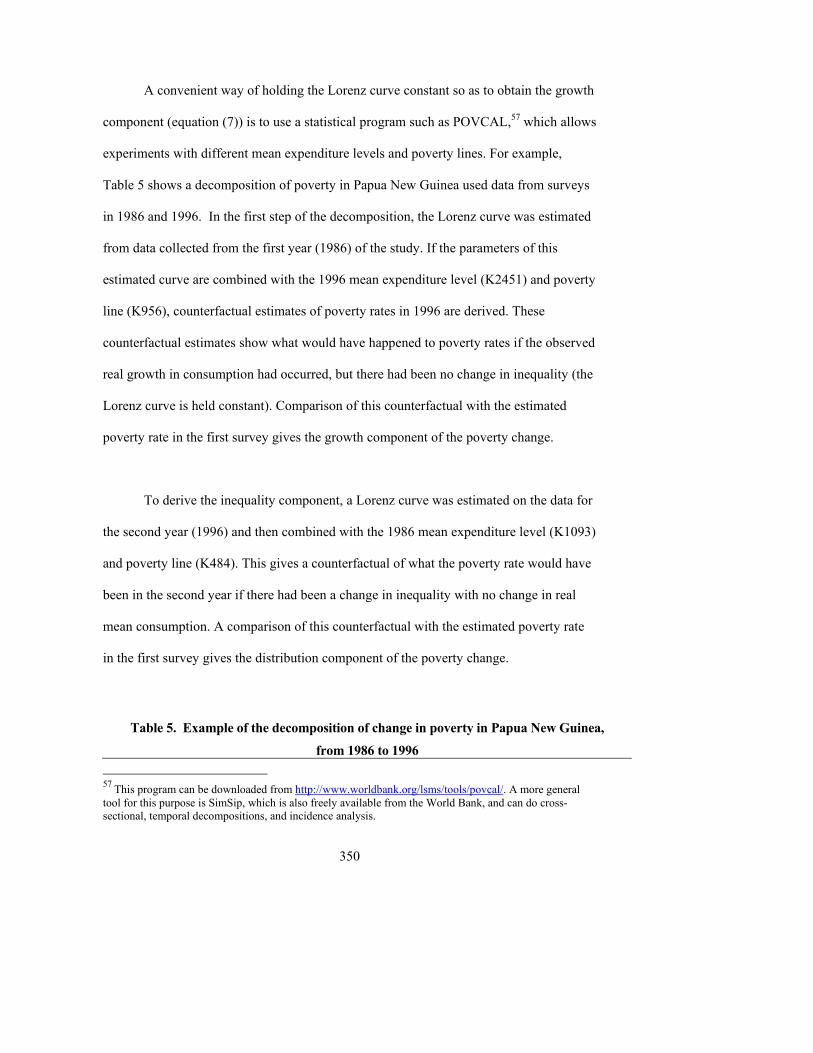
350
A convenient way of holding the Lorenz curve constant so as to obtain the growth
component (equation (7)) is to use a statistical program such as POVCAL,57 which allows
experiments with different mean expenditure levels and poverty lines. For example,
Table 5 shows a decomposition of poverty in Papua New Guinea used data from surveys
in 1986 and 1996. In the first step of the decomposition, the Lorenz curve was estimated
from data collected from the first year (1986) of the study. If the parameters of this
estimated curve are combined with the 1996 mean expenditure level (K2451) and poverty
line (K956), counterfactual estimates of poverty rates in 1996 are derived. These
counterfactual estimates show what would have happened to poverty rates if the observed
real growth in consumption had occurred, but there had been no change in inequality (the
Lorenz curve is held constant). Comparison of this counterfactual with the estimated
poverty rate in the first survey gives the growth component of the poverty change.
To derive the inequality component, a Lorenz curve was estimated on the data for
the second year (1996) and then combined with the 1986 mean expenditure level (K1093)
and poverty line (K484). This gives a counterfactual of what the poverty rate would have
been in the second year if there had been a change in inequality with no change in real
mean consumption. A comparison of this counterfactual with the estimated poverty rate
in the first survey gives the distribution component of the poverty change.
Table 5. Example of the decomposition of change in poverty in Papua New Guinea,
from 1986 to 1996 57 This program can be downloaded from http://www.worldbank.org/lsms/tools/povcal/. A more general tool for this purpose is SimSip, which is also freely available from the World Bank, and can do cross-sectional, temporal decompositions, and incidence analysis.
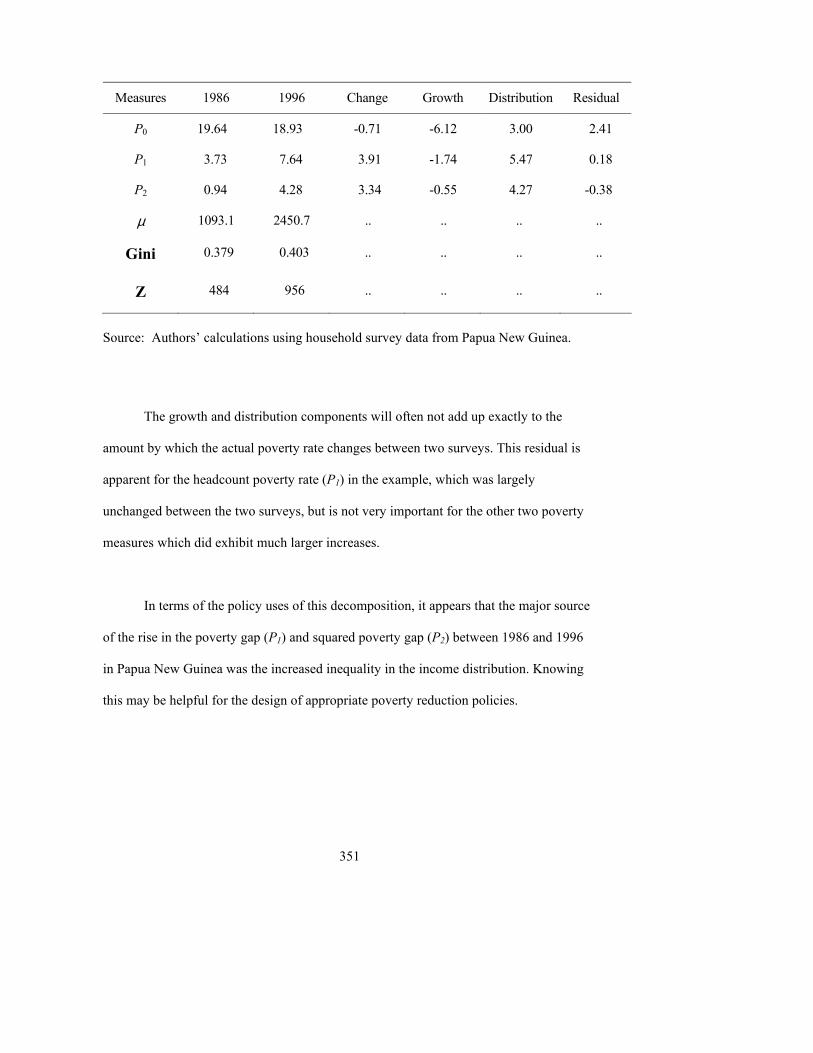
351
Measures 1986 1996 Change Growth Distribution Residual
P0 19.64 18.93 -0.71 -6.12 3.00 2.41
P1 3.73 7.64 3.91 -1.74 5.47 0.18
P2 0.94 4.28 3.34 -0.55 4.27 -0.38
µ 1093.1 2450.7 .. .. .. ..
Gini 0.379 0.403 .. .. .. ..
Z 484 956 .. .. .. ..
Source: Authors� calculations using household survey data from Papua New Guinea.
The growth and distribution components will often not add up exactly to the
amount by which the actual poverty rate changes between two surveys. This residual is
apparent for the headcount poverty rate (P1) in the example, which was largely
unchanged between the two surveys, but is not very important for the other two poverty
measures which did exhibit much larger increases.
In terms of the policy uses of this decomposition, it appears that the major source
of the rise in the poverty gap (P1) and squared poverty gap (P2) between 1986 and 1996
in Papua New Guinea was the increased inequality in the income distribution. Knowing
this may be helpful for the design of appropriate poverty reduction policies.
352
8.4.2 Panel data for two points in time This subsection relies on data from Vietnam to demonstrate how household
survey data can be used to study poverty dynamics when one has panel data for two time
periods. As in the previous subsection, the data used are from the 1992-93 and the 1997-
98 Vietnam Living Standards Surveys. This data set is of particular interest because
4,300 of the 4,800 households in the 1992-93 survey were re-interviewed in 1997-98
survey, providing a large, national representative panel data set. (In the previous
subsection these data sets were treated as repeated cross-sections.)
For simplicity, this examination of mobility and the dynamics of poverty will use
household expenditures per capita as the indicator of poverty. The poverty line used is
defined as the amount of money needed to purchase a basket of goods (both food and
nonfood) that follows typical Vietnamese expenditure patterns and provides 2,100
calories per person per day. (For further details, see, World Bank, 1999.) The panel data
reveal a poverty rate of 56.2 percent in 1992-93 and 33.5 percent in 1997-98.
Section 8.1 emphasized the key role that income (or expenditure) mobility plays
in determining poverty dynamics. Thus, the first step is to examine expenditure mobility
across the two years in Vietnam. Table 6 provides information on observed expenditure
mobility, which (as explained in Section 8.1) is likely to exaggerate the true level of
expenditure mobility. The top part of Table 6 shows a �transition matrix� that indicates,
for each of the two years, households� position across five quintiles, ranging from the
poorest 20 percent of the population (quintile 1) through the wealthiest 20 percent
(quintile 5).
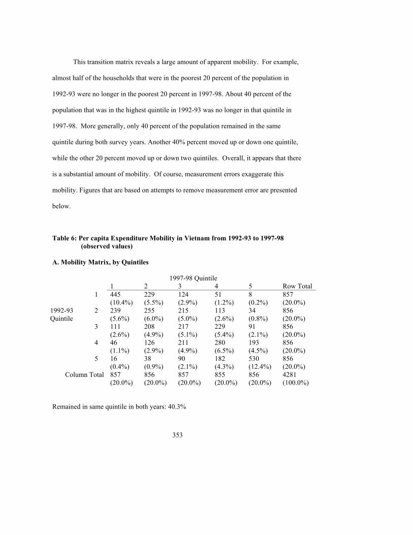
353
This transition matrix reveals a large amount of apparent mobility. For example,
almost half of the households that were in the poorest 20 percent of the population in
1992-93 were no longer in the poorest 20 percent in 1997-98. About 40 percent of the
population that was in the highest quintile in 1992-93 was no longer in that quintile in
1997-98. More generally, only 40 percent of the population remained in the same
quintile during both survey years. Another 40% percent moved up or down one quintile,
while the other 20 percent moved up or down two quintiles. Overall, it appears that there
is a substantial amount of mobility. Of course, measurement errors exaggerate this
mobility. Figures that are based on attempts to remove measurement error are presented
below.
Table 6: Per capita Expenditure Mobility in Vietnam from 1992-93 to 1997-98 (observed values)
A. Mobility Matrix, by Quintiles
1997-98 Quintile 1 2 3 4 5 Row Total 1 445
(10.4%) 229 (5.5%)
124 (2.9%)
51 (1.2%)
8 (0.2%)
857 (20.0%)
1992-93 Quintile
2 239 (5.6%)
255 (6.0%)
215 (5.0%)
113 (2.6%)
34 (0.8%)
856 (20.0%)
3 111 (2.6%)
208 (4.9%)
217 (5.1%)
229 (5.4%)
91 (2.1%)
856 (20.0%)
4 46 (1.1%)
126 (2.9%)
211 (4.9%)
280 (6.5%)
193 (4.5%)
856 (20.0%)
5 16 (0.4%)
38 (0.9%)
90 (2.1%)
182 (4.3%)
530 (12.4%)
856 (20.0%)
Column Total 857 (20.0%)
856 (20.0%)
857 (20.0%)
855 (20.0%)
856 (20.0%)
4281 (100.0%)
Remained in same quintile in both years: 40.3%
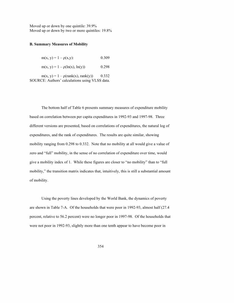
354
Moved up or down by one quintile: 39.9% Moved up or down by two or more quintiles: 19.8% B. Summary Measures of Mobility m(x, y) = 1 � ρ(x,y): 0.309 m(x, y) = 1 � ρ(ln(x), ln(y)) 0.298 m(x, y) = 1 � ρ(rank(x), rank(y)) 0.332 SOURCE: Authors� calculations using VLSS data.
The bottom half of Table 6 presents summary measures of expenditure mobility
based on correlation between per capita expenditures in 1992-93 and 1997-98. Three
different versions are presented, based on correlations of expenditures, the natural log of
expenditures, and the rank of expenditures. The results are quite similar, showing
mobility ranging from 0.298 to 0.332. Note that no mobility at all would give a value of
zero and �full� mobility, in the sense of no correlation of expenditure over time, would
give a mobility index of 1. While these figures are closer to �no mobility� than to �full
mobility,� the transition matrix indicates that, intuitively, this is still a substantial amount
of mobility.
Using the poverty lines developed by the World Bank, the dynamics of poverty
are shown in Table 7-A. Of the households that were poor in 1992-93, almost half (27.4
percent, relative to 56.2 percent) were no longer poor in 1997-98. Of the households that
were not poor in 1992-93, slightly more than one tenth appear to have become poor in
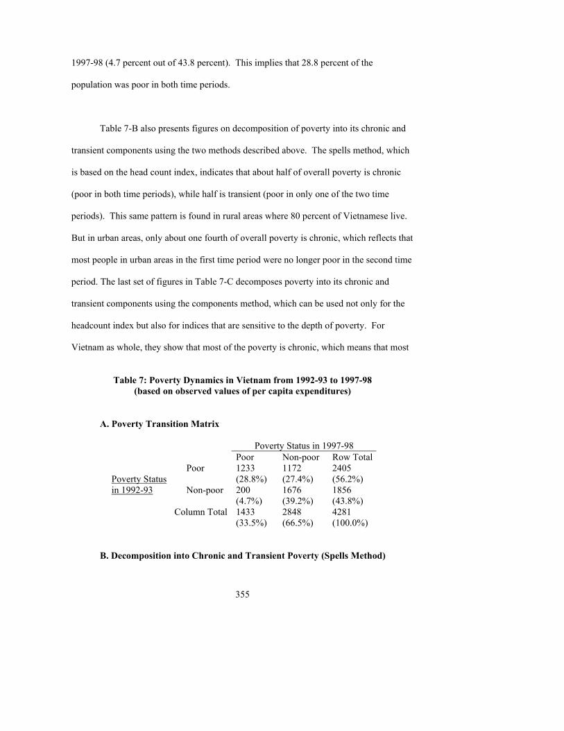
355
1997-98 (4.7 percent out of 43.8 percent). This implies that 28.8 percent of the
population was poor in both time periods.
Table 7-B also presents figures on decomposition of poverty into its chronic and
transient components using the two methods described above. The spells method, which
is based on the head count index, indicates that about half of overall poverty is chronic
(poor in both time periods), while half is transient (poor in only one of the two time
periods). This same pattern is found in rural areas where 80 percent of Vietnamese live.
But in urban areas, only about one fourth of overall poverty is chronic, which reflects that
most people in urban areas in the first time period were no longer poor in the second time
period. The last set of figures in Table 7-C decomposes poverty into its chronic and
transient components using the components method, which can be used not only for the
headcount index but also for indices that are sensitive to the depth of poverty. For
Vietnam as whole, they show that most of the poverty is chronic, which means that most
Table 7: Poverty Dynamics in Vietnam from 1992-93 to 1997-98
(based on observed values of per capita expenditures) A. Poverty Transition Matrix
Poverty Status in 1997-98 Poor Non-poor Row Total
Poor 1233 (28.8%)
1172 (27.4%)
2405 (56.2%)
Poverty Status in 1992-93
Non-poor 200 (4.7%)
1676 (39.2%)
1856 (43.8%)
Column Total 1433 (33.5%)
2848 (66.5%)
4281 (100.0%)
B. Decomposition into Chronic and Transient Poverty (Spells Method)
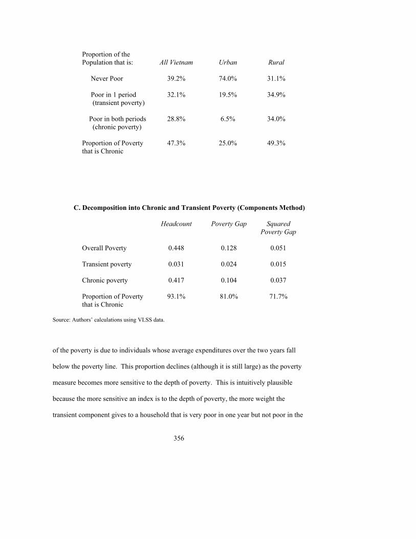
356
Proportion of the Population that is: All Vietnam Urban Rural Never Poor 39.2% 74.0% 31.1% Poor in 1 period (transient poverty)
32.1% 19.5% 34.9%
Poor in both periods (chronic poverty)
28.8% 6.5% 34.0%
Proportion of Poverty that is Chronic
47.3% 25.0% 49.3%
C. Decomposition into Chronic and Transient Poverty (Components Method)
Headcount Poverty Gap Squared Poverty Gap
Overall Poverty 0.448 0.128 0.051 Transient poverty 0.031 0.024 0.015 Chronic poverty 0.417 0.104 0.037 Proportion of Poverty that is Chronic
93.1% 81.0% 71.7%
Source: Authors� calculations using VLSS data.
of the poverty is due to individuals whose average expenditures over the two years fall
below the poverty line. This proportion declines (although it is still large) as the poverty
measure becomes more sensitive to the depth of poverty. This is intuitively plausible
because the more sensitive an index is to the depth of poverty, the more weight the
transient component gives to a household that is very poor in one year but not poor in the
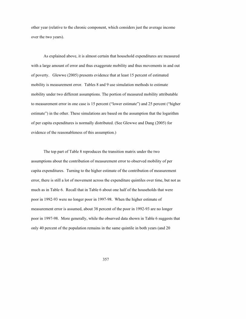
357
other year (relative to the chronic component, which considers just the average income
over the two years).
As explained above, it is almost certain that household expenditures are measured
with a large amount of error and thus exaggerate mobility and thus movements in and out
of poverty. Glewwe (2005) presents evidence that at least 15 percent of estimated
mobility is measurement error. Tables 8 and 9 use simulation methods to estimate
mobility under two different assumptions. The portion of measured mobility attributable
to measurement error in one case is 15 percent (�lower estimate�) and 25 percent (�higher
estimate�) in the other. These simulations are based on the assumption that the logarithm
of per capita expenditures is normally distributed. (See Glewwe and Dang (2005) for
evidence of the reasonableness of this assumption.)
The top part of Table 8 reproduces the transition matrix under the two
assumptions about the contribution of measurement error to observed mobility of per
capita expenditures. Turning to the higher estimate of the contribution of measurement
error, there is still a lot of movement across the expenditure quintiles over time, but not as
much as in Table 6. Recall that in Table 6 about one half of the households that were
poor in 1992-93 were no longer poor in 1997-98. When the higher estimate of
measurement error is assumed, about 38 percent of the poor in 1992-93 are no longer
poor in 1997-98. More generally, while the observed data shown in Table 6 suggests that
only 40 percent of the population remains in the same quintile in both years (and 20
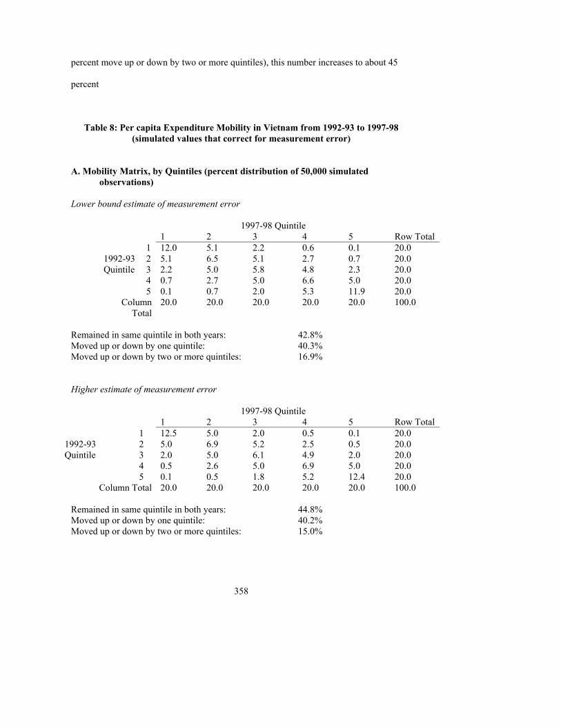
358
percent move up or down by two or more quintiles), this number increases to about 45
percent
Table 8: Per capita Expenditure Mobility in Vietnam from 1992-93 to 1997-98 (simulated values that correct for measurement error)
A. Mobility Matrix, by Quintiles (percent distribution of 50,000 simulated
observations) Lower bound estimate of measurement error
1997-98 Quintile 1 2 3 4 5 Row Total 1 12.0 5.1 2.2 0.6 0.1 20.0 1992-93 2 5.1 6.5 5.1 2.7 0.7 20.0 Quintile 3 2.2 5.0 5.8 4.8 2.3 20.0 4 0.7 2.7 5.0 6.6 5.0 20.0 5 0.1 0.7 2.0 5.3 11.9 20.0
Column Total
20.0 20.0 20.0 20.0 20.0 100.0
Remained in same quintile in both years: 42.8% Moved up or down by one quintile: 40.3% Moved up or down by two or more quintiles: 16.9% Higher estimate of measurement error
1997-98 Quintile 1 2 3 4 5 Row Total 1 12.5 5.0 2.0 0.5 0.1 20.0 1992-93 2 5.0 6.9 5.2 2.5 0.5 20.0 Quintile 3 2.0 5.0 6.1 4.9 2.0 20.0 4 0.5 2.6 5.0 6.9 5.0 20.0 5 0.1 0.5 1.8 5.2 12.4 20.0
Column Total 20.0 20.0 20.0 20.0 20.0 100.0 Remained in same quintile in both years: 44.8% Moved up or down by one quintile: 40.2% Moved up or down by two or more quintiles: 15.0%
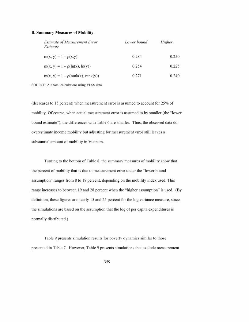
359
B. Summary Measures of Mobility Estimate of Measurement Error Lower bound Higher
Estimate m(x, y) = 1 � ρ(x,y): 0.284 0.250 m(x, y) = 1 � ρ(ln(x), ln(y)) 0.254 0.225 m(x, y) = 1 � ρ(rank(x), rank(y)) 0.271 0.240 SOURCE: Authors� calculations using VLSS data.
(decreases to 15 percent) when measurement error is assumed to account for 25% of
mobility. Of course, when actual measurement error is assumed to by smaller (the �lower
bound estimate�), the differences with Table 6 are smaller. Thus, the observed data do
overestimate income mobility but adjusting for measurement error still leaves a
substantial amount of mobility in Vietnam.
Turning to the bottom of Table 8, the summary measures of mobility show that
the percent of mobility that is due to measurement error under the �lower bound
assumption� ranges from 8 to 18 percent, depending on the mobility index used. This
range increases to between 19 and 28 percent when the �higher assumption� is used. (By
definition, these figures are nearly 15 and 25 percent for the log variance measure, since
the simulations are based on the assumption that the log of per capita expenditures is
normally distributed.)
Table 9 presents simulation results for poverty dynamics similar to those
presented in Table 7. However, Table 9 presents simulations that exclude measurement
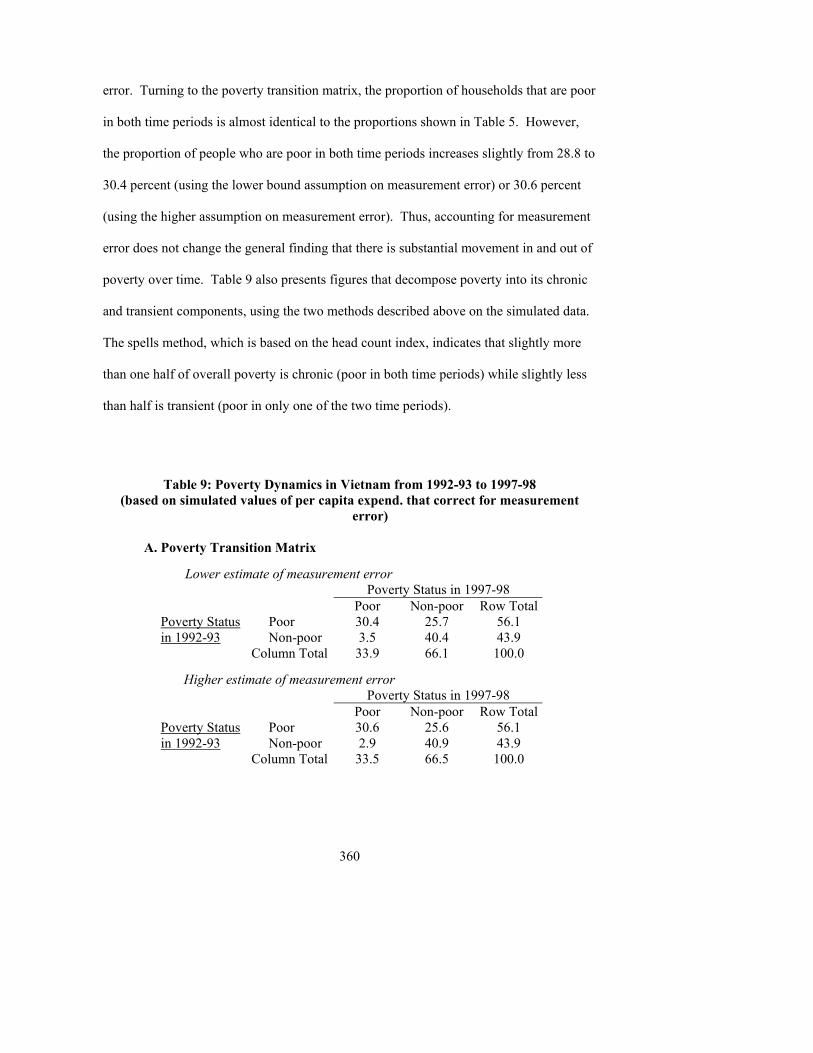
360
error. Turning to the poverty transition matrix, the proportion of households that are poor
in both time periods is almost identical to the proportions shown in Table 5. However,
the proportion of people who are poor in both time periods increases slightly from 28.8 to
30.4 percent (using the lower bound assumption on measurement error) or 30.6 percent
(using the higher assumption on measurement error). Thus, accounting for measurement
error does not change the general finding that there is substantial movement in and out of
poverty over time. Table 9 also presents figures that decompose poverty into its chronic
and transient components, using the two methods described above on the simulated data.
The spells method, which is based on the head count index, indicates that slightly more
than one half of overall poverty is chronic (poor in both time periods) while slightly less
than half is transient (poor in only one of the two time periods).
Table 9: Poverty Dynamics in Vietnam from 1992-93 to 1997-98 (based on simulated values of per capita expend. that correct for measurement
error) A. Poverty Transition Matrix Lower estimate of measurement error
Poverty Status in 1997-98 Poor Non-poor Row Total
Poor 30.4 25.7 56.1 Poverty Status in 1992-93 Non-poor 3.5 40.4 43.9
Column Total 33.9 66.1 100.0
Higher estimate of measurement error Poverty Status in 1997-98 Poor Non-poor Row Total
Poor 30.6 25.6 56.1 Poverty Status in 1992-93 Non-poor 2.9 40.9 43.9
Column Total 33.5 66.5 100.0
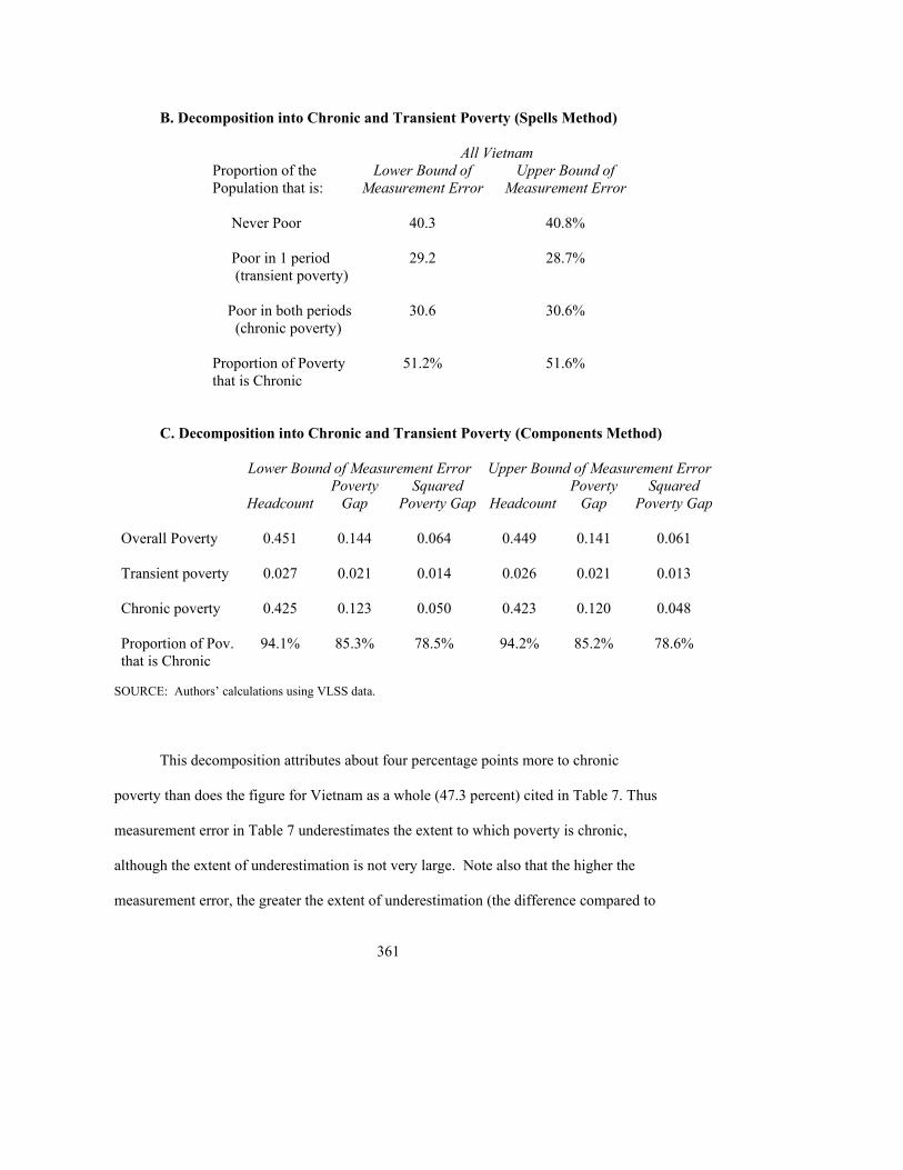
361
B. Decomposition into Chronic and Transient Poverty (Spells Method)
All Vietnam Proportion of the Population that is:
Lower Bound of Measurement Error
Upper Bound of Measurement Error
Never Poor 40.3 40.8% Poor in 1 period (transient poverty)
29.2 28.7%
Poor in both periods (chronic poverty)
30.6 30.6%
Proportion of Poverty that is Chronic
51.2% 51.6%
C. Decomposition into Chronic and Transient Poverty (Components Method) Lower Bound of Measurement Error Upper Bound of Measurement Error
Headcount Poverty
Gap Squared
Poverty Gap
HeadcountPoverty
Gap Squared
Poverty Gap Overall Poverty 0.451 0.144 0.064 0.449 0.141 0.061 Transient poverty 0.027 0.021 0.014 0.026 0.021 0.013 Chronic poverty 0.425 0.123 0.050 0.423 0.120 0.048 Proportion of Pov. that is Chronic
94.1% 85.3% 78.5% 94.2% 85.2% 78.6%
SOURCE: Authors� calculations using VLSS data.
This decomposition attributes about four percentage points more to chronic
poverty than does the figure for Vietnam as a whole (47.3 percent) cited in Table 7. Thus
measurement error in Table 7 underestimates the extent to which poverty is chronic,
although the extent of underestimation is not very large. Note also that the higher the
measurement error, the greater the extent of underestimation (the difference compared to
362
the 47.3% figure in Table 7 is 3.9% for the lower bound and 4.3% for the upper bound),
although this difference is very small. The last set of figures in Table 9 decomposes
poverty into its chronic and transient components using the components method, again
using the simulated data. For the headcount measure there is not much difference with
the poverty rate figures in Table 7. Since poverty is close to 50 percent, measurement
error is equally likely to misclassify a non-poor person as poor as it is to classify a poor
person as non-poor. However, the proportion of poverty that is chronic increases slightly,
which is consistent with the fact that measurement error tends to underestimate chronic
poverty. This underestimation of the contribution of chronic poverty to overall poverty is
even more pronounced for the measures that are sensitive to the depth of poverty.
The last issue this chapter examines using the panel data from Vietnam is if the
country�s economic growth has been �pro-poor.� This can be seen be examining growth
rates over time for each expenditure quintile. Table 10 shows this information using the
data from the 4,300 panel households. For Vietnam as a whole, per capita expenditures
rose by 41.2 percent over five years, which implies an annual rate of increase of about 7.1
percent. The remaining rows of Table 10 examine growth rates for each quintile. One
way of examining economic growth among the different expenditure quintiles is to
compare the expenditure levels of a given quintile in 1992-93 with the expenditure level
of the corresponding quintile in 1997-98, which does not necessarily compare the same
households. This can be done using both cross-sectional and panel
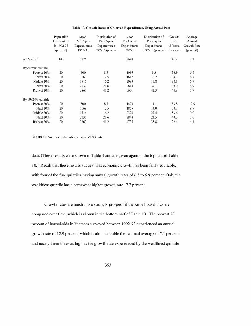
363
Table 10. Growth Rates in Observed Expenditures, Using Actual Data
Population Mean Distribution of Mean Distribution of Growth AverageDistribution Per Capita Per Capita Per Capita Per Capita over Annualin 1992-93 Expenditures Expenditures Expenditures Expenditures 5 Years Growth Rate(percent) 1992-93 1992-93 (percent) 1997-98 1997-98 (percent) (percent) (percent)
All Vietnam 100 1876 2648 41.2 7.1
By current quintilePoorest 20% 20 800 8.5 1095 8.3 36.9 6.5
Next 20% 20 1169 12.5 1617 12.2 38.3 6.7Middle 20% 20 1516 16.2 2093 15.8 38.1 6.7
Next 20% 20 2030 21.6 2840 37.1 39.9 6.9Richest 20% 20 3867 41.2 5601 42.3 44.8 7.7
By 1992-93 quintilePoorest 20% 20 800 8.5 1470 11.1 83.8 12.9
Next 20% 20 1169 12.5 1855 14.0 58.7 9.7Middle 20% 20 1516 16.2 2328 27.4 53.6 9.0
Next 20% 20 2030 21.6 2848 21.5 40.3 7.0Richest 20% 20 3867 41.2 4735 35.8 22.4 4.1
SOURCE: Authors� calculations using VLSS data.
data. (These results were shown in Table 4 and are given again in the top half of Table
10.) Recall that these results suggest that economic growth has been fairly equitable,
with four of the five quintiles having annual growth rates of 6.5 to 6.9 percent. Only the
wealthiest quintile has a somewhat higher growth rate--7.7 percent.
Growth rates are much more strongly pro-poor if the same households are
compared over time, which is shown in the bottom half of Table 10. The poorest 20
percent of households in Vietnam surveyed between 1992-93 experienced an annual
growth rate of 12.9 percent, which is almost double the national average of 7.1 percent
and nearly three times as high as the growth rate experienced by the wealthiest quintile
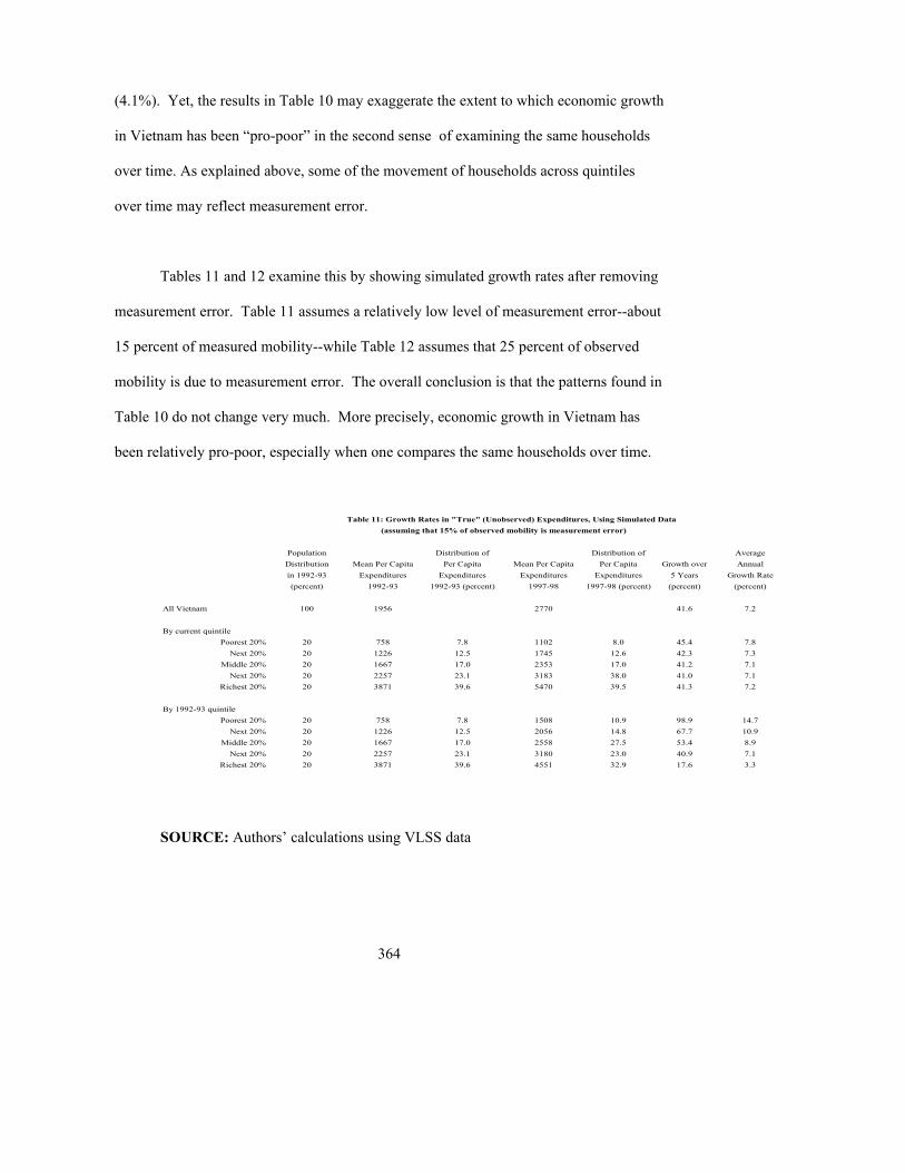
364
(4.1%). Yet, the results in Table 10 may exaggerate the extent to which economic growth
in Vietnam has been �pro-poor� in the second sense of examining the same households
over time. As explained above, some of the movement of households across quintiles
over time may reflect measurement error.
Tables 11 and 12 examine this by showing simulated growth rates after removing
measurement error. Table 11 assumes a relatively low level of measurement error--about
15 percent of measured mobility--while Table 12 assumes that 25 percent of observed
mobility is due to measurement error. The overall conclusion is that the patterns found in
Table 10 do not change very much. More precisely, economic growth in Vietnam has
been relatively pro-poor, especially when one compares the same households over time.
Table 11: Growth Rates in "True" (Unobserved) Expenditures, Using Simulated Data (assuming that 15% of observed mobility is measurement error)
Population Distribution of Distribution of AverageDistribution Mean Per Capita Per Capita Mean Per Capita Per Capita Growth over Annualin 1992-93 Expenditures Expenditures Expenditures Expenditures 5 Years Growth Rate(percent) 1992-93 1992-93 (percent) 1997-98 1997-98 (percent) (percent) (percent)
All Vietnam 100 1956 2770 41.6 7.2
By current quintilePoorest 20% 20 758 7.8 1102 8.0 45.4 7.8
Next 20% 20 1226 12.5 1745 12.6 42.3 7.3Middle 20% 20 1667 17.0 2353 17.0 41.2 7.1
Next 20% 20 2257 23.1 3183 38.0 41.0 7.1Richest 20% 20 3871 39.6 5470 39.5 41.3 7.2
By 1992-93 quintilePoorest 20% 20 758 7.8 1508 10.9 98.9 14.7
Next 20% 20 1226 12.5 2056 14.8 67.7 10.9Middle 20% 20 1667 17.0 2558 27.5 53.4 8.9
Next 20% 20 2257 23.1 3180 23.0 40.9 7.1Richest 20% 20 3871 39.6 4551 32.9 17.6 3.3
SOURCE: Authors� calculations using VLSS data
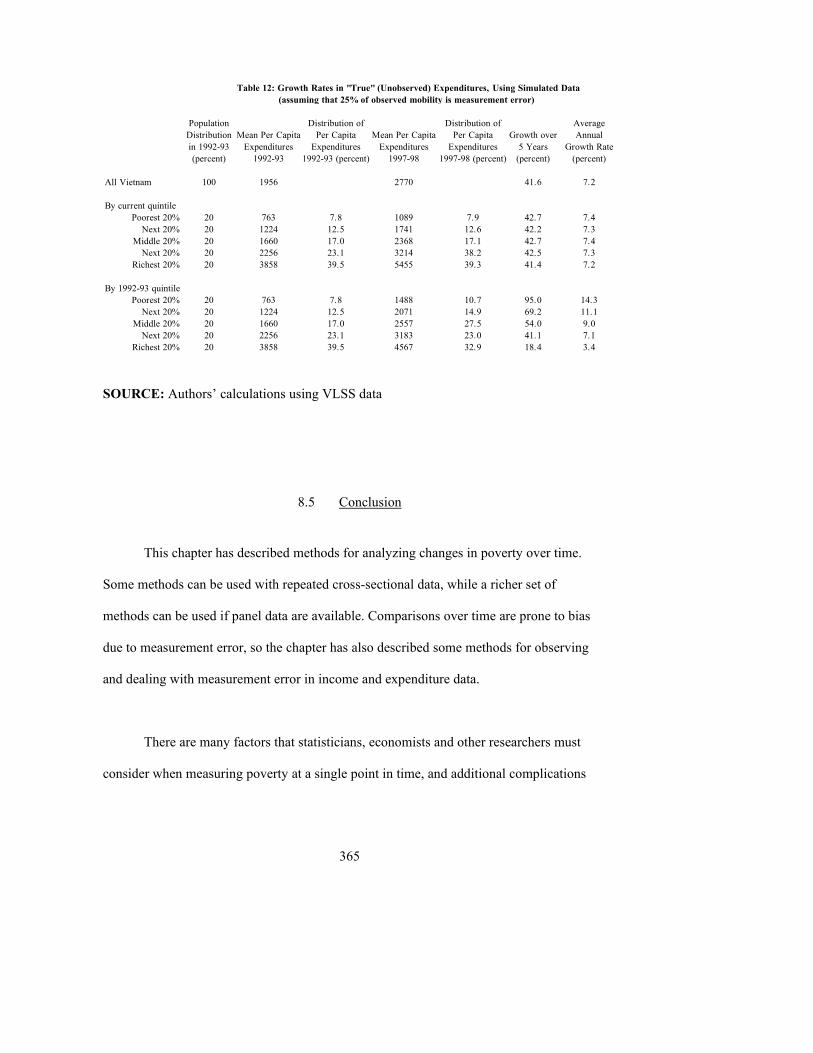
365
Table 12: Growth Rates in "True" (Unobserved) Expenditures, Using Simulated Data (assuming that 25% of observed mobility is measurement error)
Population Distribution of Distribution of AverageDistribution Mean Per Capita Per Capita Mean Per Capita Per Capita Growth over Annualin 1992-93 Expenditures Expenditures Expenditures Expenditures 5 Years Growth Rate(percent) 1992-93 1992-93 (percent) 1997-98 1997-98 (percent) (percent) (percent)
All Vietnam 100 1956 2770 41.6 7.2
By current quintilePoorest 20% 20 763 7.8 1089 7.9 42.7 7.4
Next 20% 20 1224 12.5 1741 12.6 42.2 7.3Middle 20% 20 1660 17.0 2368 17.1 42.7 7.4
Next 20% 20 2256 23.1 3214 38.2 42.5 7.3Richest 20% 20 3858 39.5 5455 39.3 41.4 7.2
By 1992-93 quintilePoorest 20% 20 763 7.8 1488 10.7 95.0 14.3
Next 20% 20 1224 12.5 2071 14.9 69.2 11.1Middle 20% 20 1660 17.0 2557 27.5 54.0 9.0
Next 20% 20 2256 23.1 3183 23.0 41.1 7.1Richest 20% 20 3858 39.5 4567 32.9 18.4 3.4
SOURCE: Authors� calculations using VLSS data
8.5 Conclusion
This chapter has described methods for analyzing changes in poverty over time.
Some methods can be used with repeated cross-sectional data, while a richer set of
methods can be used if panel data are available. Comparisons over time are prone to bias
due to measurement error, so the chapter has also described some methods for observing
and dealing with measurement error in income and expenditure data.
There are many factors that statisticians, economists and other researchers must
consider when measuring poverty at a single point in time, and additional complications
366
arise when examining how poverty changes over time. This paper has reviewed three
important conceptual issues:
• Relationship between poverty dynamics and income mobility,
• Chronic poverty vs. transient poverty, and
• How to measure the impact of economic growth on the poor.
Two important data issues were also addressed:
• Relative merits of cross-sectional and panel data, and
• Problems due to measurement error.
This chapter provides lessons for statistical agencies in developed and developing
countries on how to collect data that are useful for understanding the dynamics of
poverty. Because poverty and poverty dynamics may vary significantly from country to
country, and because most poor nations have only limited data � in particular, most lack
panel data � it is not possible to draw general policy conclusions or even general
conclusions about the nature of poverty dynamics. However, if this chapter�s survey
recommendations are followed, then each country will have the data necessary to
understand poverty dynamics and to formulate poverty-reducing policies.
Perhaps the most important data collection recommendation is that all countries
should attempt to collect nationally representative panel data. It may not be necessary to
visit households every year; every two or three years may yield sufficiently useful data.
(For detailed recommendations on collecting panel data, see Glewwe and Jacoby, 2000.)
367
The second key lesson is that measurement error is a serious problem that can lead to
biased results. National statistical agencies should undertake comprehensive efforts to
improve the accuracy of their household survey data, such as increasing supervision of
field work and conducting validation studies. A third lesson is that there are methods that
can be used to minimize bias due to measurement error when analyzing poverty data.
Study of poverty dynamics in both developed and developing countries is a
relatively new area of research. Much more thinking is needed to refine underlying
theoretical concepts, and to improve data collection and analysis. Statisticians,
economists, and other researchers need to work together with statistical agencies to learn
more about poverty dynamics in both developed and developing countries. This will lead
to more effective poverty policies and, ultimately, to less poverty.
368
References Baulch, Bob, and John Hoddinott. 2000. �Economic Mobility and Poverty Dynamics in Developing Countries� Journal of Development Studies 36(6):1-24. Bound, John, and Alan Krueger. 1991. �The Extent of Measurement Error in Longitudinal Earnings Data: Do Two Wrongs Make a Right?� Journal of Labor Economics 9(1):1-24. Cappellari, Lorenzo, and Stephen Jenkins. 2002. �Who Stays Poor, Who Becomes Poor? Evidence from the British Household Panel Survey� Economic Journal 112(478)C60-C67. Datt, Gaurav, and Martin Ravallion. 1992. �Growth and Redistribution Components of Changes in Poverty Measures: A Decomposition with Applications to Brazil and India in the 1980s� Journal of Development Economics 38(2):275-295. Falaris, Evangelos. 2003. �The Effect of Survey Attrition in Longitudinal Surveys: Evidence from Peru, Côte d�Ivoire and Vietnam� Journal of Development Economics 70(1):133-157. Fitzgerald, John, Peter Gottschalk and Robert Moffitt. 1998. �An Analysis of Panel Attrition in Panel Data� Journal of Human Resources 33(2):251-299.
Gibson, John. 2000. The impact of growth and distribution on poverty in Papua New Guinea . Applied Economics Letters 7(8): 541-544.
Glewwe, Paul. 2005. �How Much of Observed Economic Mobility is Measurement Error? A Method to Reduce Measurement Error, with an Application to Vietnam�. Department of Applied Economics, University of Minnesota. Glewwe, Paul, and Hai-Anh Dang. 2005. �Has Vietnam�s Economic Growth in the 1990�s Been Pro-Poor? An Analysis of Data from the Vietnam Living Standards Surveys�. Department of Applied Economics, University of Minnesota. Glewwe, Paul, and Hanan Jacoby, 2000. �Recommendations for Collecting Panel Data�, in M. Grosh and P. Glewwe, eds., Designing Household Survey Questionnaires for Developing Countries: Lessons from 15 Years of the Living Standards Measurement Study. Oxford University Press for the World Bank. Heise, David. 1969. �Separating Reliability and Stability in Test-Retest Correlation� American Sociological Review 34(1):93-101. Jalan, Jyotsna, and Martin Ravallion. 1998. �Transient Poverty in Post-Reform Rural China� Journal of Comparative Economics 26(2):338-357.
369
Pischke, Jörn-Steffen. 1995. �Measurement Error and Earnings Dynamics: Some Estimates from the PSID Validation Study� Journal of Business and Economic Statistics. 13(3):305-314. Thomas, Duncan, Elizabeth Frankenberg and James Smith. 2001. �Lost, but not Forgotten: Attrition in the Indonesian Family Life Survey� Journal of Human Resources 36(3)556-592. World Bank. 1999. �Vietnam: Attacking Poverty� Hanoi. World Bank. 2001. �Vietnam Living Standards Survey (VLSS), 1997-98: Basic Information�. Policy Research Group. The World Bank, Washington DC (available on the web at http://www.worldbank.org/lsms/country/vn98/vn98bif.pdf).
370
CHAPTER IX. CONCLUSION
Gisele Kamanou
Anecdotal evidence is critical for understanding the human side of poverty.
However, sound statistical data and analysis are essential for accurately assessing the full
dimension of poverty and to gauge the impact of anti-poverty programs
As this handbook has extensively revealed, measuring poverty is not a simple
matter. Even within a single nation�s borders, the metrics of poverty can vary
significantly between city and country, between single and multi-person households, and
in grey markets where individuals may be reticent to disclose their full income. In the
most extreme cases, it may be impossible for country�s to find and survey its poorest
because of a lack of permanent residence or respondents� inability to clearly answer
questions.
9.1 Summary
A key goal of this handbook has been to find common ground in the ways
countries measure poverty and to make recommendations that increase harmonization of
these practices. The handbook has identified aspects in poverty measurement where
371
improvements are essential. Monetary measurements, for example, should base the
measurement of welfare on expenditures data as opposed to income data. They should
follow the same standards in establishing poverty lines, in adjusting for adult equivalent,
and in conducting poverty-focused household surveys (including collecting price data and
handling missing data and implausibly low values of income and consumption).
The handbook encourages similar improvements in adopting a broad set of
guidelines for poverty analysis to achieve more consistent and reliable interpretation of
raw data. For example, as a practical recommendation, it is suggested to focus on
producing the most commonly used poverty measures (i.e., the headcount index, poverty
gap, and squared poverty gap) to promote comparability across countries. Other
measures, such as the median income of the poor population, that are simple to compute
and provide a richer picture of conditions of poverty, should also be computed more
frequently than is currently the practice.
There has been considerable improvement in poverty measurement over the
recent decades. However, countries should make effort in following some basic steps to
further improve the reliability and comparability of the basic poverty data, for example,
using multiple thresholds that include a common value, e.g. 2,100 kcalories. The choice
of divisor for calculating per capita poverty figures can also significantly affect the
results. Developing countries need technical assistance in applying scale economy-
adjusted methods for estimating per capita household food consumption and income
(expenditure) distributions. More specifically, further empirical work is needed that lead
372
to evidence-based recommendations on the use of the age-by-sex RDA in estimating
food-poverty lines and on the use of models to incorporate scale economies in deriving
divisors for computing per capita non-food poverty lines and income/expenditures.
Another theme of this handbook is the need for consistent survey methods so that
poverty comparisons uncover real changes in the population rather than statistical
distortions caused by variations in survey design. The method of data capture employed
in the poverty surveys varies greatly among countries, from one-year, six month or one
month recall of income and expenditures to a daily diary method supplemented by
weekly recall. Overall, sensitivity of poverty estimates to variations in survey design also
underscores the importance of measurement error. Comparisons over time are
particularly prone to bias due to measurement error. Furthermore, many country- and
community-based poverty evaluation and monitoring systems lack consistency because
they are launched by donors and external agencies possessing the necessary seed funds
but lacking concern for a coordinated focus. They do not usually fit together in terms of
their scope, timing, and coverage. Many will have been implemented as one-off
exercises or prove unsustainable for either technical or financial reasons.
National statistical agencies should undertake comprehensive efforts to improve
the accuracy of their household survey data, such as increasing supervision of field work
and conducting validation studies. Along the same line, converging data-capture
methods used by developing countries, supported by empirical evidence from
experiments imbedded in the poverty surveys themselves, should be a high priority in
373
national and international programs. As part of a more comprehensive probability-based
survey design, alternative sources (including qualitative and subjective methods and
national accounts) can provide more insightful poverty assessments. International
agencies and other organizations should give high priority to developing global
household survey standards to generate reliable poverty estimates consistent with the
national accounts across countries and across time. Further, it is crucially important that
all countries attempt to collect nationally representative panel data, even if this means
revisiting households only every two or three years.
9.2 Statistical addendum: The UN Global survey on poverty measurement practices
A number of nations have problems aggregating basic poverty data � including
data from different regions--to produce an accurate picture of its own poverty. Such
difficulties grow exponentially when trying to assess poverty across borders. Only by
identifying similarities and differences in the ways in which nations collect data, can we
begin to understand the accuracy of poverty studies. This is the purpose of the statistical
addendum presented in the Annex 3. Data collection methods and poverty statistics
presented are the product of a year-long study that sought to enhance the understanding
of both the character of poverty and the ways in which nations measure it. In gaining a
clearer understanding of how poverty is measured, this report will help identify the
strengths and weaknesses in the current data collection processes.
374
The genesis of this survey started in May 2004 in Rio de Janeiro, Brazil with the
first United Nations workshop on poverty measurements. Subsequent workshops were
held in July 2004 in Abuja, Nigeria, in October 2004 in Manila, Philippines, and then in
November 2004 in Amman, Jordan that refined the questionnaire, paving the way for the
first global survey of how nations measure poverty. The survey had two primary
purposes: discover regional perspectives in how nations gauge poverty and identify
means in which poverty measurement could be improved.
After being translated into English, Spanish, French and Russian, the
questionnaire was sent out in February 2005 to national statistical offices in nearly 189
countries around the world. To help obtain a greater response rate, the UN prepared an
abridged version of the questionnaire which was sent out to countries in October 2005.
All together, Government statistical offices in 106 countries replied to the global survey.
Statistical offices in 15 countries indicated that they are not currently collecting poverty
data at all.
Survey responses were subsequently consolidated in the statistical addendum
highlight the substantial areas where greater uniformity will raise the overall quality of
poverty measure and improve comparability of measures across time and location. If
nations embrace this report�s survey recommendations, it may ensure a more accurate
understanding of poverty and help produce more comparable national statistics. If these
goals can be achieved, they will ultimately help nations more effectively target spending
and ameliorate poverty.
375
ANNEXES
A.1 List of the United Nations Steering Committee on Poverty Statistics
Patricia Alexander, Regional Advisor on Poverty Statistics Statistics Division, Economic and Social Commission for Asia and Pacific, United Nations, Bangkok, Thailand Isidoro P. David, Consultant 16 Whitefield White Plains Subdivision Quezon City, Metro-Manila, Philippines Martin Balepa, Directeur General AFRISTAT, Bamako, Mali Christian N. Grootaert International development Consultant for The World Bank and IRIS Center McLean, USA Ivo C. Havinga, Chief, Economic Statistics Branch United Nations Statistics Division, United Nations, New York, USA Pali Lehohla, Statistician-General Statistics South Africa Pretoria, South Africa Choiril Maksumo, Director General BPS � Statistics Indonesia Jakarta, Indonesia Jonathan Morduch (Chair of the Steering Committee), Professor of Public Policy and Economics, NYU Wagner School New York, USA Eduardo Pereira Nunes, President Fundaçao I B G E Rio de Janeiro, Brazil Sanjay G. Reddy, Assistant Professor Department of Economics, Barnard College, Columbia University New York, USA Pedro Sainz , CEPAL
376
Casilla 179-D Santiago, CHILE Michael Ward 2a, Waddelow Road, Waterbeach Cambridge, United Kingdom
377
A.2 List of the countries who participated in the regional workshops on poverty measurement
Economic Commission for Latin America and the Caribbean (ECLAC) Region Argentina, Brazil, Bahamas, Barbados, Bolivia, Chile, Colombia, Dominica, Ecuador, Grenada, Peru, St. Lucia, Jamaica, Mexico, Paraguay, Uruguay Economic and Social Commission for Asia and the Pacific (ESCAP) Region Bangladesh, Cambodia, Canada, China, Fiji, Indonesia, Islamic Republic of Iran, Republic of Korea, Lao PDR, Macao China, Maldives, Mongolia, Papua New Guinea, , Philippines, Sri Lanka, Thailand, Vietnam Economic Commission for Western Asia Region Egypt, Iraq, Lebanon, Jordan, Oman, Palestine, Syria Economic Community of West African States (ECOWAS) Region and few countries from other parts of Africa Benin, Burkina Faso, Cape Verde, Cote d�Ivoire, Ghana, Guinea Bissau, Liberia, Niger, Senegal, Sierra Leone, Togo, and Angola, Cameroon, Gabon Rwanda, Tanzania
378
A.3 Questionnaire of the UN Global Survey of poverty measurement practices and Statistical addendum
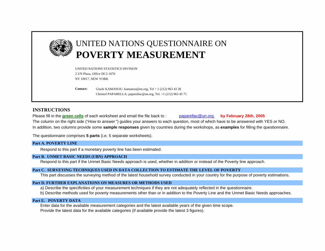
UNITED NATIONS QUESTIONNAIRE ONPOVERTY MEASUREMENTUNITED NATIONS STATISTICS DIVISION2 UN Plaza, Office DC2-1676NY 10017, NEW YORK
Contact: Gisele KAMANOU: [email protected], Tel + 1 (212) 963 43 28Christof PAPARELLA: [email protected], Tel. +1 (212) 963 45 71
INSTRUCTIONSPlease fill in the green cells of each worksheet and email the file back to : [email protected] by February 28th, 2005The column on the right side (“How to answer ”) guides your answers to each question, most of which have to be answered with YES or NO. In addition, two columns provide some sample responses given by countries during the workshops, as examples for filling the questionnaire.
The questionnaire comprises 5 parts (i.e. 5 separate worksheets).
Part A. POVERTY LINERespond to this part if a monetary poverty line has been estimated.
Part B. UNMET BASIC NEEDS (UBN) APPROACHRespond to this part if the Unmet Basic Needs approach is used, whether in addition or instead of the Poverty line approach.
Part C. SURVEYING TECHNIQUES USED IN DATA COLLECTION TO ESTIMATE THE LEVEL OF POVERTYThis part discusses the surveying method of the latest household survey conducted in your country for the purpose of poverty estimations.
Part D. FURTHER EXPLANATIONS ON MEASURES OR METHODS USEDa) Describe the specificities of your measurement techniques if they are not adequately reflected in the questionnaire.b) Describe methods used for poverty measurements other than or in addition to the Poverty Line and the Unmet Basic Needs approaches.
Part E. POVERTY DATAEnter data for the available measurement categories and the latest available years of the given time scope. Provide the latest data for the available categories (if available provide the latest 3 figures).
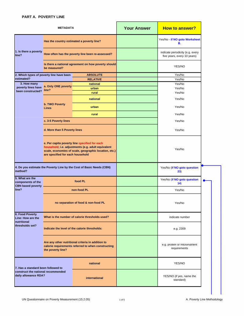
PART A. POVERTY LINE
Your Answer How to answer?
Yes/No - if NO goto Worksheet B.
indicate periodicity (e.g. every five years, every 10 years)
YES/NO
ABSOLUTE Yes/NoRELATIVE Yes/Nonational Yes/Nourban Yes/Norural Yes/No
national Yes/No
urban Yes/No
rural Yes/No
Yes/No
Yes/No
Yes/No
Yes/No (if NO goto question 23)
Yes/No (if NO goto question 14)
Yes/No
Yes/No
indicate number
e.g. 2309
e.g. protein or micronutrient requirements
national YES/NO
international YES/NO (if yes, name the standard)
What is the number of calorie thresholds used?
Indicate the level of the calorie thresholds:
Are any other nutritional criteria in addition to calorie requirements referred to when constructing the poverty line?
1. Is there a poverty line?
Has the country estimated a poverty line?
How often has the poverty line been re-assessed?
Is there a national agreement on how poverty should be measured?
METADATA
e. Per capita poverty line specified for each household; i.e. adjustments (e.g. adult equivalent scale, economies of scale, geographic location, etc.) are specified for each household
2. Which types of poverty line have been estimated?
7. Has a standard been followed to construct the national recommended daily allowance RDA?
a. Only ONE poverty line?
3. How many poverty lines have been constructed?
b. TWO Poverty Lines
c. 3-5 Poverty lines
d. More than 5 Poverty lines
no separation of food & non-food PL
4. Do you estimate the Poverty Line by the Cost of Basic Needs (CBN) method?
5. What are the components of the CBN based poverty line?
food PL
non-food PL
6. Food Poverty Line: How are the nutritional thresholds set?
UN Questionnaire on Poverty Measurement (15.2.05) 1 of 5 A. Poverty Line Methodology
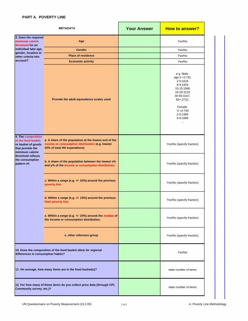
PART A. POVERTY LINE
Your Answer How to answer? METADATA
Yes/No
Yes/No
Yes/No
Yes/No
e.g. Male: age 0 <2:791
2-5:16186-9:1924
10-15:199016-29:321630-59:3167,60+:2710.
Female:
0 <2:7402-5:14806-9:1689
...
Yes/No (specify fraction)
Yes/No (specify fraction)
Yes/No (specify fraction)
Yes/No (specify fraction)
Yes/No (specify fraction)
Yes/No (specify fraction)
Yes/No
state number of items
state number of items
Place of residence
8. Does the required minimum calorie threshold for an individual take age, gender, location or other criteria into account?
Gender
Economic activity
Provide the adult equivalence scales used
Age
e. Within a range (e.g. +/- 10%) around the median of the income or consumption distribution.
12. For how many of these items do you collect price data (through CPI, Community survey, etc.)?
10. Does the composition of the food basket allow for regional differences in consumption habits?
b. A share of the population between the lowest x% and y% of the income or consumption distribution.
11. On average, how many items are in the food basket(s)?
c. Within a range (e.g. +/- 10%) around the previous poverty line.
9. The composition of the food basket or basket of goods that provide the minimum calorie threshold reflects the consumption pattern of:
a. A share of the population at the lowest end of the income or consumption distribution (e.g. lowest 20% of total HH expenditure)
d. Within a range (e.g. +/- 10%) around the previous food poverty line.
e. other reference group
UN Questionnaire on Poverty Measurement (15.2.05) 2 of 5 A. Poverty Line Methodology
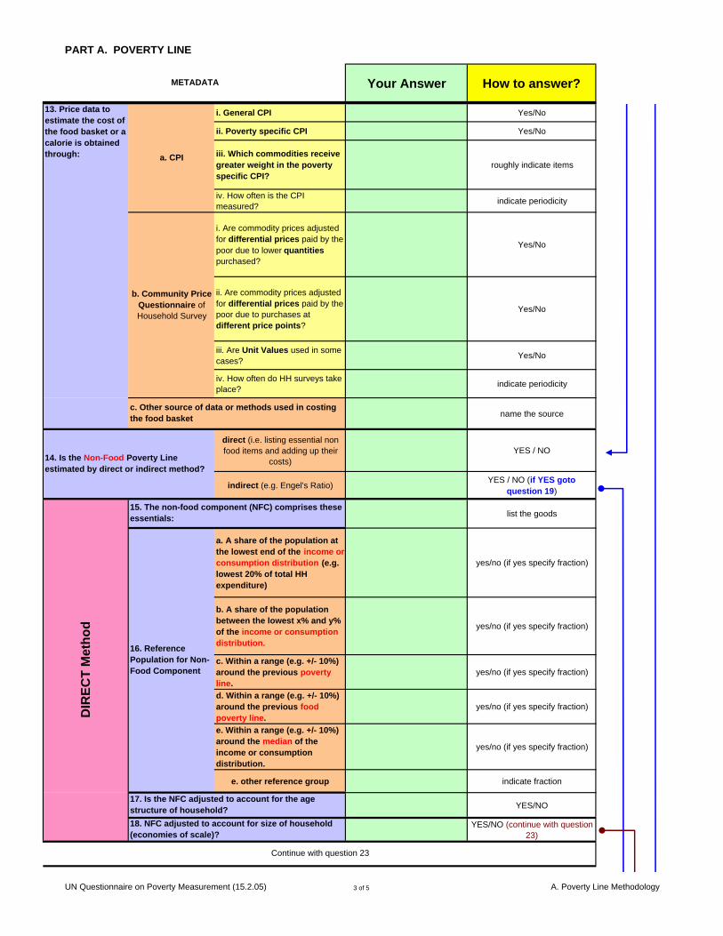
PART A. POVERTY LINE
Your Answer How to answer? METADATA
i. General CPI Yes/No
ii. Poverty specific CPI Yes/No
iii. Which commodities receive greater weight in the poverty specific CPI?
roughly indicate items
iv. How often is the CPI measured? indicate periodicity
i. Are commodity prices adjusted for differential prices paid by the poor due to lower quantities purchased?
Yes/No
ii. Are commodity prices adjusted for differential prices paid by the poor due to purchases at different price points?
Yes/No
iii. Are Unit Values used in some cases? Yes/No
iv. How often do HH surveys take place? indicate periodicity
name the source
direct (i.e. listing essential non food items and adding up their
costs)YES / NO
indirect (e.g. Engel's Ratio) YES / NO (if YES goto question 19)
list the goods
a. A share of the population at the lowest end of the income or consumption distribution (e.g. lowest 20% of total HH expenditure)
yes/no (if yes specify fraction)
b. A share of the population between the lowest x% and y% of the income or consumption distribution.
yes/no (if yes specify fraction)
c. Within a range (e.g. +/- 10%) around the previous poverty line.
yes/no (if yes specify fraction)
d. Within a range (e.g. +/- 10%) around the previous food poverty line.
yes/no (if yes specify fraction)
e. Within a range (e.g. +/- 10%) around the median of the income or consumption distribution.
yes/no (if yes specify fraction)
e. other reference group indicate fraction
YES/NO
YES/NO (continue with question 23)
15. The non-food component (NFC) comprises these essentials:
c. Other source of data or methods used in costing the food basket
17. Is the NFC adjusted to account for the age structure of household?18. NFC adjusted to account for size of household (economies of scale)?
Continue with question 23
16. Reference Population for Non-Food Component
13. Price data to estimate the cost of the food basket or a calorie is obtained through:
b. Community Price Questionnaire of Household Survey
DIR
ECT
Met
hod
a. CPI
14. Is the Non-Food Poverty Line estimated by direct or indirect method?
UN Questionnaire on Poverty Measurement (15.2.05) 3 of 5 A. Poverty Line Methodology
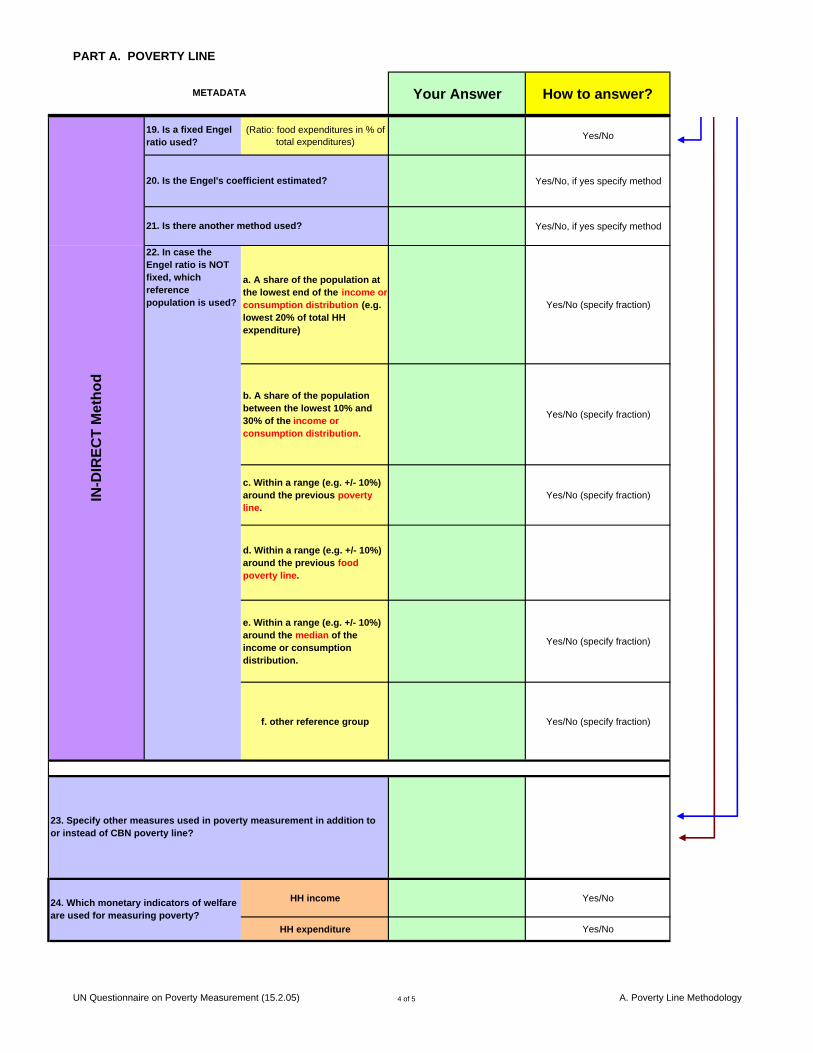
PART A. POVERTY LINE
Your Answer How to answer? METADATA
19. Is a fixed Engel ratio used?
(Ratio: food expenditures in % of total expenditures) Yes/No
Yes/No, if yes specify method
Yes/No, if yes specify method
a. A share of the population at the lowest end of the income or consumption distribution (e.g. lowest 20% of total HH expenditure)
Yes/No (specify fraction)
b. A share of the population between the lowest 10% and 30% of the income or consumption distribution.
Yes/No (specify fraction)
c. Within a range (e.g. +/- 10%) around the previous poverty line.
Yes/No (specify fraction)
d. Within a range (e.g. +/- 10%) around the previous food poverty line.
e. Within a range (e.g. +/- 10%) around the median of the income or consumption distribution.
Yes/No (specify fraction)
f. other reference group Yes/No (specify fraction)
HH income Yes/No
HH expenditure Yes/No
20. Is the Engel's coefficient estimated?
21. Is there another method used?
IN-D
IREC
T M
etho
d
22. In case the Engel ratio is NOT fixed, which reference population is used?
24. Which monetary indicators of welfare are used for measuring poverty?
23. Specify other measures used in poverty measurement in addition to or instead of CBN poverty line?
UN Questionnaire on Poverty Measurement (15.2.05) 4 of 5 A. Poverty Line Methodology
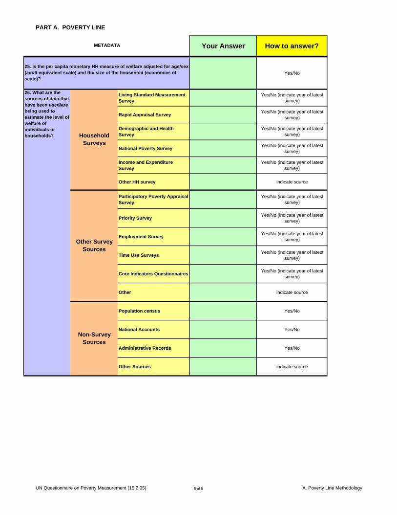
PART A. POVERTY LINE
Your Answer How to answer? METADATA
Yes/No
Living Standard Measurement Survey
Yes/No (indicate year of latest survey)
Rapid Appraisal Survey Yes/No (indicate year of latest survey)
Demographic and Health Survey
Yes/No (indicate year of latest survey)
National Poverty Survey Yes/No (indicate year of latest survey)
Income and Expenditure Survey
Yes/No (indicate year of latest survey)
Other HH survey indicate source
Participatory Poverty Appraisal Survey
Yes/No (indicate year of latest survey)
Priority Survey Yes/No (indicate year of latest survey)
Employment Survey Yes/No (indicate year of latest survey)
Time Use Surveys Yes/No (indicate year of latest survey)
Core Indicators Questionnaires Yes/No (indicate year of latest survey)
Other indicate source
Population census Yes/No
National Accounts Yes/No
Administrative Records Yes/No
Other Sources indicate source
Household Surveys
26. What are the sources of data that have been used/are being used to estimate the level of welfare of individuals or households?
Non-Survey Sources
25. Is the per capita monetary HH measure of welfare adjusted for age/sex (adult equivalent scale) and the size of the household (economies of scale)?
Other Survey Sources
UN Questionnaire on Poverty Measurement (15.2.05) 5 of 5 A. Poverty Line Methodology
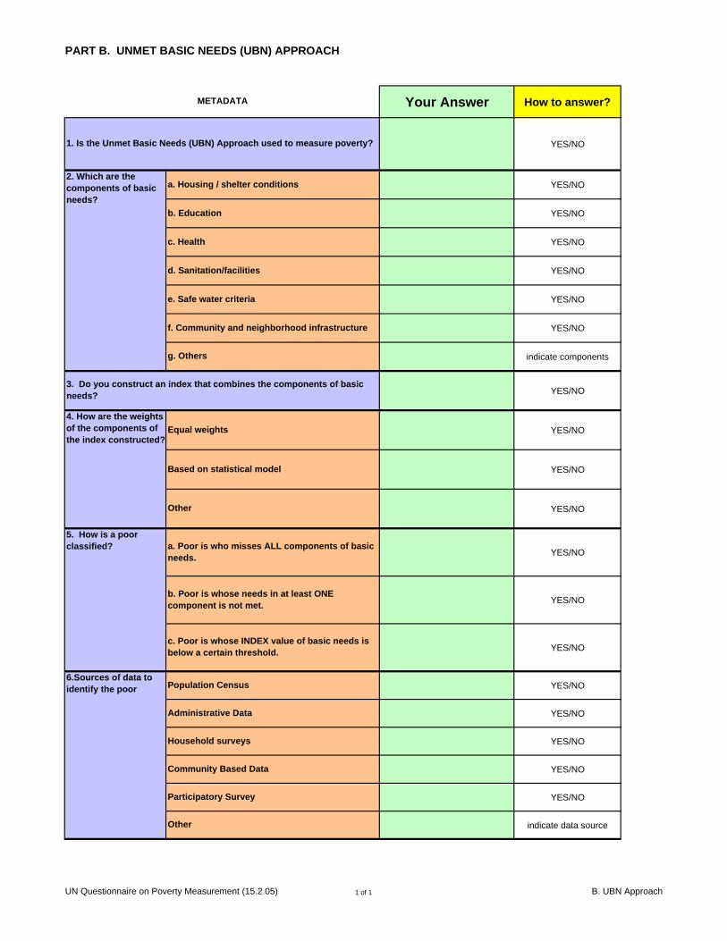
PART B. UNMET BASIC NEEDS (UBN) APPROACH
Your Answer How to answer?
YES/NO
YES/NO
YES/NO
YES/NO
YES/NO
YES/NO
YES/NO
indicate components
YES/NO
YES/NO
YES/NO
YES/NO
YES/NO
YES/NO
YES/NO
YES/NO
YES/NO
YES/NO
YES/NO
YES/NO
indicate data source
b. Poor is whose needs in at least ONE component is not met.
5. How is a poor classified?
4. How are the weights of the components of the index constructed?
Equal weights
Based on statistical model
Other
e. Safe water criteria
f. Community and neighborhood infrastructure
METADATA
1. Is the Unmet Basic Needs (UBN) Approach used to measure poverty?
a. Housing / shelter conditions
b. Education
c. Health
d. Sanitation/facilities
2. Which are the components of basic needs?
g. Others
3. Do you construct an index that combines the components of basic needs?
6.Sources of data to identify the poor Population Census
Administrative Data
Household surveys
Community Based Data
Participatory Survey
Other
c. Poor is whose INDEX value of basic needs is below a certain threshold.
a. Poor is who misses ALL components of basic needs.
UN Questionnaire on Poverty Measurement (15.2.05) 1 of 1 B. UBN Approach
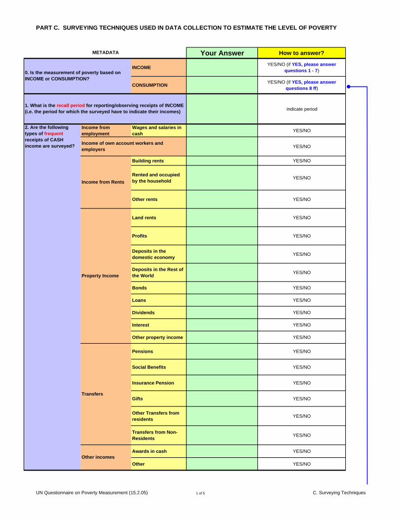
PART C. SURVEYING TECHNIQUES USED IN DATA COLLECTION TO ESTIMATE THE LEVEL OF POVERTY
Your Answer How to answer?
INCOME YES/NO (if YES, please answer questions 1 - 7)
CONSUMPTION YES/NO (if YES, please answer questions 8 ff)
indicate period
Income from employment
Wages and salaries in cash YES/NO
YES/NO
Building rents YES/NO
Rented and occupied by the household YES/NO
Other rents YES/NO
Land rents YES/NO
Profits YES/NO
Deposits in the domestic economy YES/NO
Deposits in the Rest of the World YES/NO
Bonds YES/NO
Loans YES/NO
Dividends YES/NO
Interest YES/NO
Other property income YES/NO
Pensions YES/NO
Social Benefits YES/NO
Insurance Pension YES/NO
Gifts YES/NO
Other Transfers from residents YES/NO
Transfers from Non-Residents YES/NO
Awards in cash YES/NO
Other YES/NO
0. Is the measurement of poverty based on INCOME or CONSUMPTION?
METADATA
Income from Rents
Property Income
Transfers
Other incomes
Income of own account workers and employers
1. What is the recall period for reporting/observing receipts of INCOME (i.e. the period for which the surveyed have to indicate their incomes)
2. Are the following types of frequent receipts of CASH income are surveyed?
UN Questionnaire on Poverty Measurement (15.2.05) 1 of 5 C. Surveying Techniques
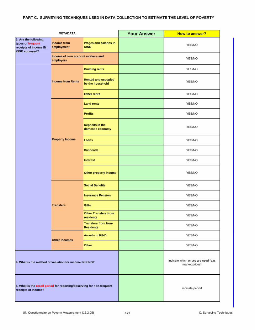
PART C. SURVEYING TECHNIQUES USED IN DATA COLLECTION TO ESTIMATE THE LEVEL OF POVERTY
Your Answer How to answer? METADATA
Income from employment
Wages and salaries in KIND YES/NO
YES/NO
Building rents YES/NO
Rented and occupied by the household YES/NO
Other rents YES/NO
Land rents YES/NO
Profits YES/NO
Deposits in the domestic economy YES/NO
Loans YES/NO
Dividends YES/NO
Interest YES/NO
Other property income YES/NO
Social Benefits YES/NO
Insurance Pension YES/NO
Gifts YES/NO
Other Transfers from residents YES/NO
Transfers from Non-Residents YES/NO
Awards in KIND YES/NO
Other YES/NO
indicate which prices are used (e.g. market prices)
indicate period5. What is the recall period for reporting/observing for non-frequent receipts of income?
Income from Rents
Income of own account workers and employers
4. What is the method of valuation for income IN KIND?
3. Are the following types of frequent receipts of income IN KIND surveyed?
Property Income
Transfers
Other incomes
UN Questionnaire on Poverty Measurement (15.2.05) 2 of 5 C. Surveying Techniques
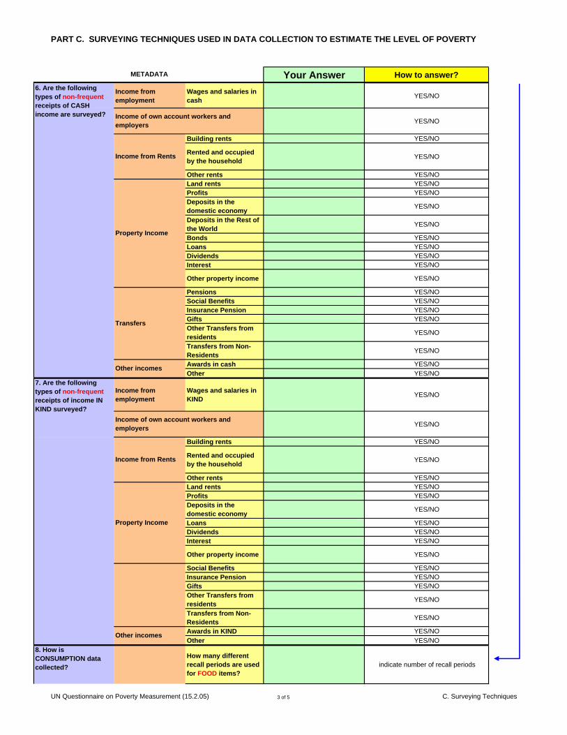
PART C. SURVEYING TECHNIQUES USED IN DATA COLLECTION TO ESTIMATE THE LEVEL OF POVERTY
Your Answer How to answer? METADATA
Income from employment
Wages and salaries in cash YES/NO
YES/NO
Building rents YES/NO
Rented and occupied by the household YES/NO
Other rents YES/NOLand rents YES/NOProfits YES/NODeposits in the domestic economy YES/NO
Deposits in the Rest of the World YES/NO
Bonds YES/NOLoans YES/NODividends YES/NOInterest YES/NO
Other property income YES/NO
Pensions YES/NOSocial Benefits YES/NOInsurance Pension YES/NOGifts YES/NOOther Transfers from residents YES/NO
Transfers from Non-Residents YES/NO
Awards in cash YES/NOOther YES/NO
Income from employment
Wages and salaries in KIND YES/NO
YES/NO
Building rents YES/NO
Rented and occupied by the household YES/NO
Other rents YES/NOLand rents YES/NOProfits YES/NODeposits in the domestic economy YES/NO
Loans YES/NODividends YES/NOInterest YES/NO
Other property income YES/NO
Social Benefits YES/NOInsurance Pension YES/NOGifts YES/NOOther Transfers from residents YES/NO
Transfers from Non-Residents YES/NO
Awards in KIND YES/NOOther YES/NO
How many different recall periods are used for FOOD items?
indicate number of recall periods
Income of own account workers and employers
7. Are the following types of non-frequent receipts of income IN KIND surveyed?
Income from Rents
Property Income
Other incomes
Income from Rents
Property Income
Transfers
Other incomes
6. Are the following types of non-frequent receipts of CASH income are surveyed?
Income of own account workers and employers
8. How is CONSUMPTION data collected?
UN Questionnaire on Poverty Measurement (15.2.05) 3 of 5 C. Surveying Techniques
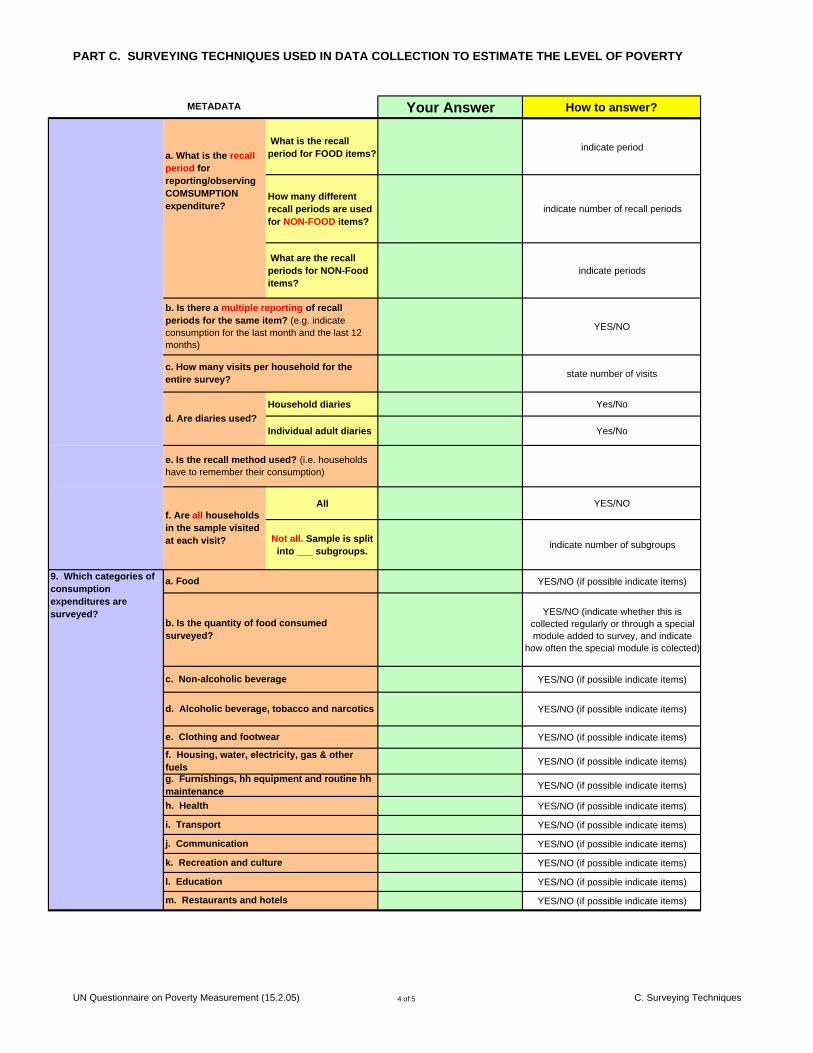
PART C. SURVEYING TECHNIQUES USED IN DATA COLLECTION TO ESTIMATE THE LEVEL OF POVERTY
Your Answer How to answer? METADATA
What is the recall period for FOOD items? indicate period
How many different recall periods are used for NON-FOOD items?
indicate number of recall periods
What are the recall periods for NON-Food items?
indicate periods
YES/NO
state number of visits
Household diaries Yes/No
Individual adult diaries Yes/No
All YES/NO
Not all. Sample is split into ___ subgroups. indicate number of subgroups
YES/NO (if possible indicate items)
YES/NO (indicate whether this is collected regularly or through a special module added to survey, and indicate
how often the special module is colected)
YES/NO (if possible indicate items)
YES/NO (if possible indicate items)
YES/NO (if possible indicate items)
YES/NO (if possible indicate items)
YES/NO (if possible indicate items)
YES/NO (if possible indicate items)
YES/NO (if possible indicate items)
YES/NO (if possible indicate items)
YES/NO (if possible indicate items)
YES/NO (if possible indicate items)
YES/NO (if possible indicate items)
f. Housing, water, electricity, gas & other fuels
m. Restaurants and hotels
9. Which categories of consumption expenditures are surveyed?
a. Food
c. Non-alcoholic beverage
d. Alcoholic beverage, tobacco and narcotics
j. Communication
g. Furnishings, hh equipment and routine hh maintenanceh. Health
e. Clothing and footwear
b. Is the quantity of food consumed surveyed?
i. Transport
k. Recreation and culture
l. Education
b. Is there a multiple reporting of recall periods for the same item? (e.g. indicate consumption for the last month and the last 12 months)
d. Are diaries used?
c. How many visits per household for the entire survey?
e. Is the recall method used? (i.e. households have to remember their consumption)
f. Are all households in the sample visited at each visit?
a. What is the recall period for reporting/observing COMSUMPTION expenditure?
UN Questionnaire on Poverty Measurement (15.2.05) 4 of 5 C. Surveying Techniques
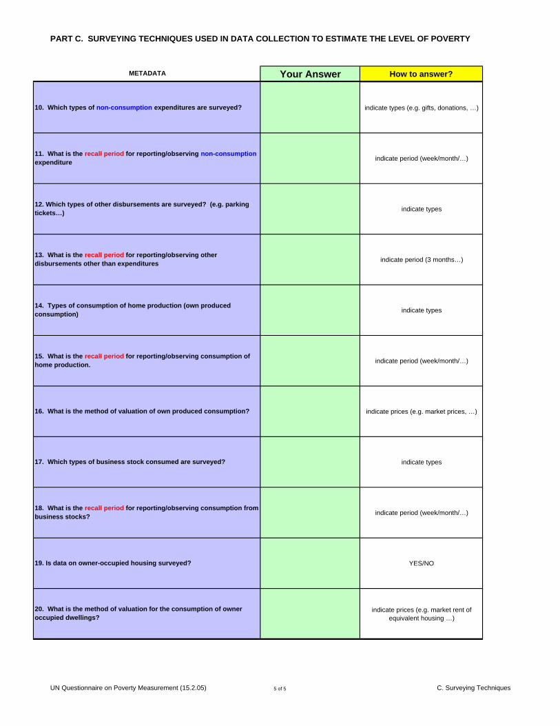
PART C. SURVEYING TECHNIQUES USED IN DATA COLLECTION TO ESTIMATE THE LEVEL OF POVERTY
Your Answer How to answer? METADATA
indicate types (e.g. gifts, donations, …)
indicate period (week/month/…)
indicate types
indicate period (3 months…)
indicate types
indicate period (week/month/…)
indicate prices (e.g. market prices, …)
indicate types
indicate period (week/month/…)
YES/NO
indicate prices (e.g. market rent of equivalent housing …)
11. What is the recall period for reporting/observing non-consumption expenditure
20. What is the method of valuation for the consumption of owner occupied dwellings?
14. Types of consumption of home production (own produced consumption)
16. What is the method of valuation of own produced consumption?
18. What is the recall period for reporting/observing consumption from business stocks?
17. Which types of business stock consumed are surveyed?
12. Which types of other disbursements are surveyed? (e.g. parking tickets…)
19. Is data on owner-occupied housing surveyed?
10. Which types of non-consumption expenditures are surveyed?
13. What is the recall period for reporting/observing other disbursements other than expenditures
15. What is the recall period for reporting/observing consumption of home production.
UN Questionnaire on Poverty Measurement (15.2.05) 5 of 5 C. Surveying Techniques
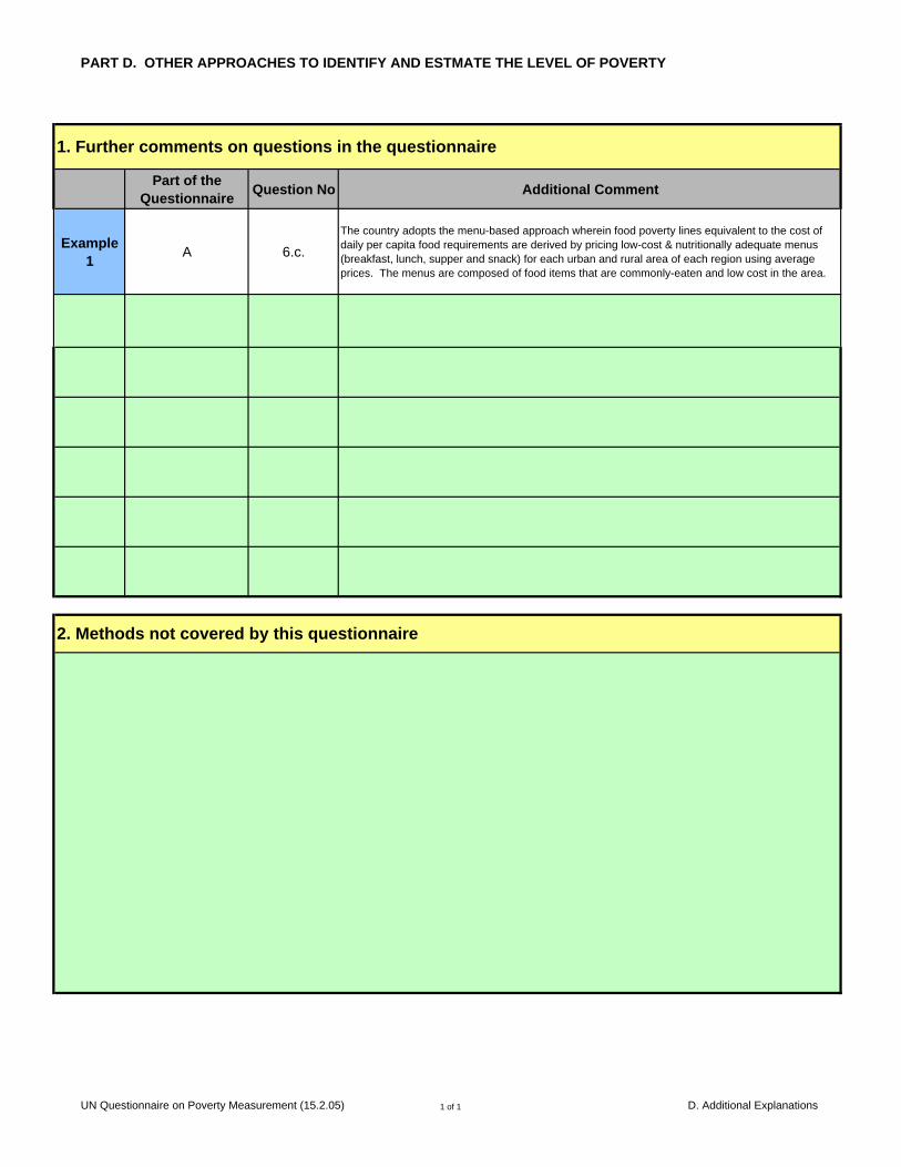
PART D. OTHER APPROACHES TO IDENTIFY AND ESTMATE THE LEVEL OF POVERTY
Part of the Questionnaire Question No Additional Comment
Example 1 A 6.c.
The country adopts the menu-based approach wherein food poverty lines equivalent to the cost of daily per capita food requirements are derived by pricing low-cost & nutritionally adequate menus (breakfast, lunch, supper and snack) for each urban and rural area of each region using average prices. The menus are composed of food items that are commonly-eaten and low cost in the area.
1. Further comments on questions in the questionnaire
2. Methods not covered by this questionnaire
UN Questionnaire on Poverty Measurement (15.2.05) 1 of 1 D. Additional Explanations
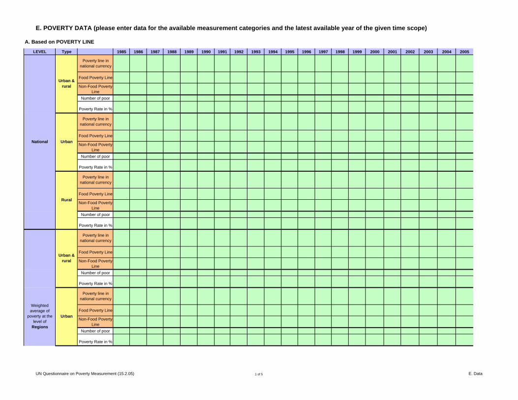
E. POVERTY DATA (please enter data for the available measurement categories and the latest available year of the given time scope)
LEVEL Type 1985 1986 1987 1988 1989 1990 1991 1992 1993 1994 1995 1996 1997 1998 1999 2000 2001 2002 2003 2004 2005
Poverty line in national currency
Food Poverty Line
Non-Food Poverty Line
Number of poor
Poverty Rate in %
Poverty line in national currency
Food Poverty Line
Non-Food Poverty Line
Number of poor
Poverty Rate in %
Poverty line in national currency
Food Poverty Line
Non-Food Poverty Line
Number of poor
Poverty Rate in %
Poverty line in national currency
Food Poverty Line
Non-Food Poverty Line
Number of poor
Poverty Rate in %
Poverty line in national currency
Food Poverty Line
Non-Food Poverty Line
Number of poor
Poverty Rate in %
A. Based on POVERTY LINE
National
Urban & rural
Urban
Rural
Weighted average of
poverty at the level of
Regions
Urban & rural
Urban
UN Questionnaire on Poverty Measurement (15.2.05) 1 of 5 E. Data
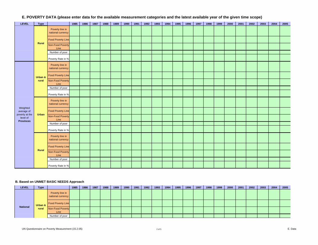
E. POVERTY DATA (please enter data for the available measurement categories and the latest available year of the given time scope)LEVEL Type 1985 1986 1987 1988 1989 1990 1991 1992 1993 1994 1995 1996 1997 1998 1999 2000 2001 2002 2003 2004 2005
Poverty line in national currency
Food Poverty Line
Non-Food Poverty Line
Number of poor
Poverty Rate in %
Poverty line in national currency
Food Poverty Line
Non-Food Poverty Line
Number of poor
Poverty Rate in %
Poverty line in national currency
Food Poverty Line
Non-Food Poverty Line
Number of poor
Poverty Rate in %
Poverty line in national currency
Food Poverty Line
Non-Food Poverty Line
Number of poor
Poverty Rate in %
LEVEL Type 1985 1986 1987 1988 1989 1990 1991 1992 1993 1994 1995 1996 1997 1998 1999 2000 2001 2002 2003 2004 2005
Poverty line in national currency
Food Poverty Line
Non-Food Poverty Line
Number of poor
B. Based on UNMET BASIC NEEDS Approach
Urban & ruralNational
Rural
Weighted average of
poverty at the level of
Provinces
Urban & rural
Urban
Rural
UN Questionnaire on Poverty Measurement (15.2.05) 2 of 5 E. Data
E. POVERTY DATA (please enter data for the available measurement categories and the latest available year of the given time scope)LEVEL Type 1985 1986 1987 1988 1989 1990 1991 1992 1993 1994 1995 1996 1997 1998 1999 2000 2001 2002 2003 2004 2005
Poverty Rate in %
UN Questionnaire on Poverty Measurement (15.2.05) 3 of 5 E. Data
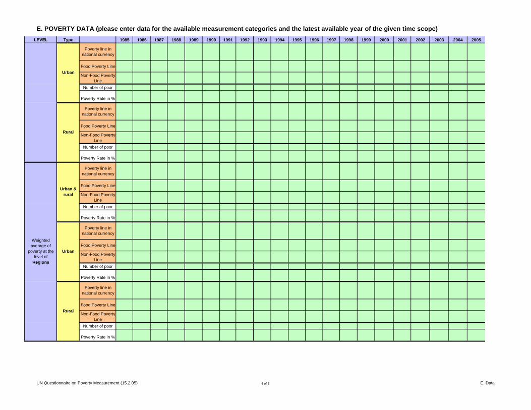
E. POVERTY DATA (please enter data for the available measurement categories and the latest available year of the given time scope)LEVEL Type 1985 1986 1987 1988 1989 1990 1991 1992 1993 1994 1995 1996 1997 1998 1999 2000 2001 2002 2003 2004 2005
Poverty line in national currency
Food Poverty Line
Non-Food Poverty Line
Number of poor
Poverty Rate in %
Poverty line in national currency
Food Poverty Line
Non-Food Poverty Line
Number of poor
Poverty Rate in %
Poverty line in national currency
Food Poverty Line
Non-Food Poverty Line
Number of poor
Poverty Rate in %
Poverty line in national currency
Food Poverty Line
Non-Food Poverty Line
Number of poor
Poverty Rate in %
Poverty line in national currency
Food Poverty Line
Non-Food Poverty Line
Number of poor
Poverty Rate in %
Weighted average of
poverty at the level of
Regions
Urban & rural
Urban
Rural
Urban
Rural
UN Questionnaire on Poverty Measurement (15.2.05) 4 of 5 E. Data
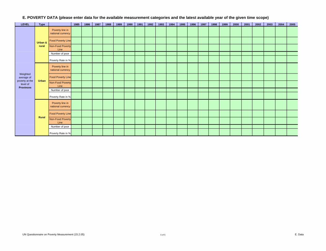
E. POVERTY DATA (please enter data for the available measurement categories and the latest available year of the given time scope)LEVEL Type 1985 1986 1987 1988 1989 1990 1991 1992 1993 1994 1995 1996 1997 1998 1999 2000 2001 2002 2003 2004 2005
Poverty line in national currency
Food Poverty Line
Non-Food Poverty Line
Number of poor
Poverty Rate in %
Poverty line in national currency
Food Poverty Line
Non-Food Poverty Line
Number of poor
Poverty Rate in %
Poverty line in national currency
Food Poverty Line
Non-Food Poverty Line
Number of poor
Poverty Rate in %
Weighted average of
poverty at the level of
Provinces
Urban & rural
Urban
Rural
UN Questionnaire on Poverty Measurement (15.2.05) 5 of 5 E. Data
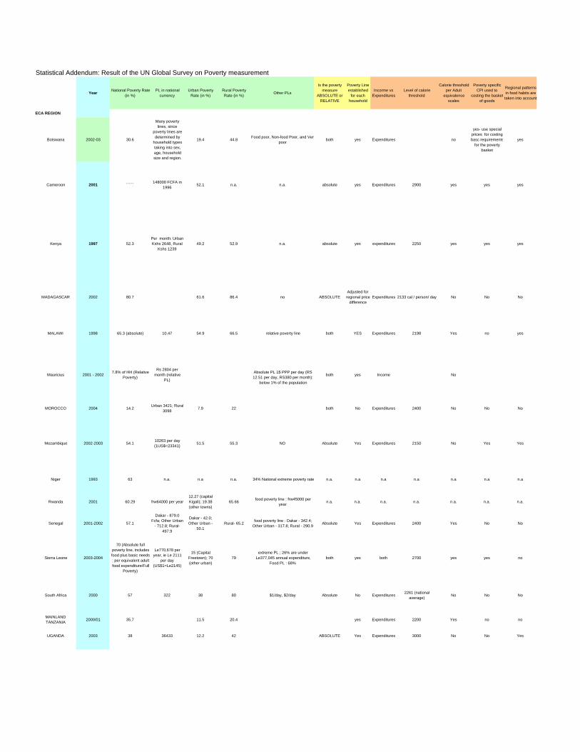
Statistical Addendum: Result of the UN Global Survey on Poverty measurement
Year National Poverty Rate (in %)
PL in national currency
Urban Poverty Rate (in %)
Rural Poverty Rate (in %) Other PLs
Is the poverty measure
ABSOLUTE or RELATIVE
Poverty Line established
for each household
Incorme vs Expenditures
Level of calorie threshold
Calorie threshold per Adult
equivalence scales
Poverty specific CPI used to
costing the basketof goods
Regional patterns in food habits are taken into account
ECA REGION
Botswana 2002-03 30.6
Many poverty lines, since
poverty lines are determined by
household types taking into sex, age, household size and region.
19.4 44.8 Food poor, Non-food Poor, and Verypoor both yes Expenditures no
yes- use special prices for costing basc requirements
for the poverty basket
yes
Cameroon 2001 `````` 148000 FCFA in 1996 52.1 n.a. n.a. absolute yes Expenditures 2900 yes yes yes
Kenya 1997 52.3Per month: UrbanKshs 2648, Rural
Kshs 123949.2 52.9 n.a. absolute yes expenditures 2250 yes yes yes
MADAGASCAR 2002 80.7 61.6 86.4 no ABSOLUTEAdjusted for regional price
differenceExpenditures 2133 cal / person/ day No No No
MALAWI 1998 65.3 (absolute) 10.47 54.9 66.5 relative poverty line both YES Expenditures 2198 Yes no yes
Mauricius 2001 - 2002 7.8% of HH (Relative Poverty)
Rs 2804 per month (relative
PL)
Absolute PL 1$ PPP per day (RS 12.51 per day, RS380 per month):
below 1% of the population
both yes Income No
MOROCCO 2004 14.2 Urban 3421; Rural3098 7.9 22 both No Expenditures 2400 No No No
Mozambique 2002-2003 54.1 10263 per day (1US$=23341) 51.5 55.3 NO Absolute Yes Expenditures 2150 No Yes Yes
Niger 1993 63 n.a. n.a n.a. 34% National extreme poverty rate n.a. n.a n.a n.a n.a n.a n.a
Rwanda 2001 60.29 frw64000 per year12.27 (capital Kigali); 19.38 (other towns)
65.66 food poverty line : frw45000 per year n.a. n.a. n.a. n.a. n.a. n.a. n.a.
Senegal 2001-2002 57.1
Dakar - 879.0 Fcfa; Other Urban
- 712.8; Rural-497.9
Dakar - 42.0; Other Urban -
50.1Rural- 65.2 food poverty line : Dakar - 342.4;
Other Urban - 317.8; Rural - 290.9 Absolute Yes Expenditures 2400 Yes No No
Sierra Leone 2003-2004
70 (Absolute full poverty line, includes food plus basic needs : per equivalent adult food expenditure/Full
Poverty)
Le770,678 per year, ie Le 2111
per day (US$1=Le2145)
15 (Capital Freetown); 70 (other urban)
79extreme PL ; 26% are under
Le377,045 annual expenditure, Food PL : 68%
both yes both 2700 yes yes no
South Africa 2000 57 322 38 80 $1/day, $2/day Absolute No Expenditures 2261 (national average) No No No
MAINLAND TANZANIA 2000/01 35.7 11.5 20.4 yes Expenditures 2200 Yes no no
UGANDA 2003 38 36433 12.2 42 ABSOLUTE Yes Expenditures 3000 No No Yes
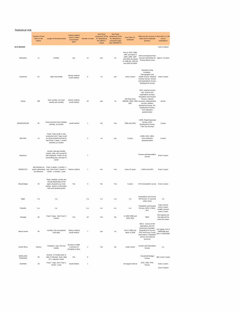
Statistical Add
ECA REGION
Botswana
Cameroon
Kenya
MADAGASCAR
MALAWI
Mauricius
MOROCCO
Mozambique
Niger
Rwanda
Senegal
Sierra Leone
South Africa
MAINLAND TANZANIA
UGANDA
Number of food items in the
basketLength of Recall period(s)
Diaries method used to collect consumption
data?
Number of visits
Non-Food component of the PL obtained by
the DIRECT metod
Non-Food component of the PL obtained by using the Engel
ratio (INDIRECT)
How Often PL estimated
What are the sources ofdata used to estimate
poverty?
How often is a HHsurvey
undertaken?
none of above
11 monthly yes 12 yes no
First in 1976, 1989, 1997 and latest is 2003. 1989, 1997
and 2003 are based on 1985-86, 1993-94and 2002-03 HIES
HIES and Special Price Surveys specifically for Poverty datum Lines
approx. 10 years
61 daily and weekly Diaries method, recall method, 6 no yes every 5 years
Standard Living Condition ,
Demographic and Health Survey, National Poverty Survey, Incomeand Expenditure Survey
Employment Survey
every 5 years
100 food: weekly; non food: weekly and monthly
Diaries method, recall method 10 yes no
Not fixed since 1981/82, 1992, 1994,
1997
DHS, national poverty and income and
expenditure surveys, Population and Housing
Census, national accounts, administrative
records, Welfare Monitoring Survey, PA, Employment Survey,
Core indicators questionnaire;
ad hoc
82 Food and Non Food: Weeklymonthly, 12 months recall method 1 No Yes 1993 and 2001
LSMS, Rapid Appraisal Survey, DHS,
Employment Survey, Time Use Surveys
2 years
14
Food: 3 day recall on own production and 7 days recall on all purchased food items, Non Food: 1 week, 1 month,
3months,12 months
2 no yes 5 yearsLSMS, DHS, HIES,
Core Indicators Questionnaires
5 years
Income: last pay (montly, weekly, daily, etc) except for self employed, it refers to lasaccounting year, and past 12
month
7 Income and ExpenditureSurvey Every 5 years
Nb d'articles du panier alimentaire
de référence
Food: 2 weeks, 2 months, 1 year, Non Food: 2 weeks, 1 month , 3 months, 1 year
Diaries method 7 No Yes every 10 years LSMS and HIES Every 5 years
40
Daily, weekely, montly and annual depending on the types of goods (e.g. food,
cloting, leisure or edcucationfees and durable goods)
Yes 3 No Yes 5 years HH Consumption survey Every 5 years
n.a n.a n.a n.a n.a n.aExpenditure and IncomeHH Survey, in rural and
urban areasn.a
n.a. n.a. n.a. n.a. n.a. n.a.Population and HousingCensus, MICS, CWIQ,
SLC
huge surveys every 5 years,
smaller surveys every 2 years
26 Food: 3 days, Non Food: 4 months Yes 10 Yes No In 1994-1995 and
2001-2002 HIESNot regulary but now planned for every five years
40 monthly, then annualized; food daily
Diaries method, recall method 7 yes no first in 1990 and
latest in 2004
MICS, Survey of HH Ependiture and HH
Economics Activities, Integrated HH Survey, PPA and Focus Group
Discussions, Populationcensus and national
accounts
not regular, first in1989/1990 and
then in 2003/2004
Various Durables 1 year, the rest montly
No diary in 2000. In process of
changing to diary.2 Yes No under review Income and Expenditure
Survey n.a.
28Income: 12 months prior to date of interview, food: daily
for 1 calender monthYes 8 Household Budget
Survey after every 5 years
28 Food: 7 days, Non Food: 1 month, 1 year recall method 1 No regular interval DHS, HIES, PPA
Survey Every 2 years
none of above
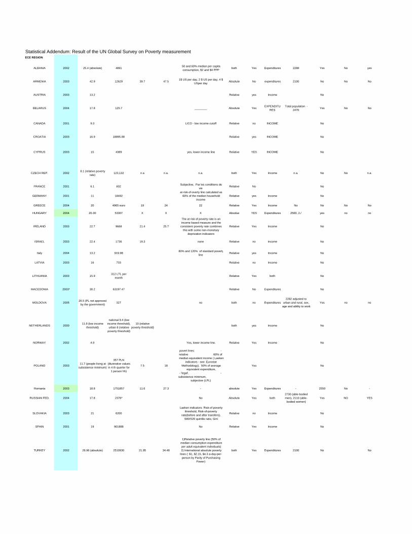
Statistical Addendum: Result of the UN Global Survey on Poverty measurementECE REGION
ALBANIA 2002 25.4 (absolute) 4891 50 and 60% median per capita consumption, $2 and $4 PPP both Yes Expenditures 2288 Yes No yes
ARMENIA 2003 42.9 12629 39.7 47.5 1$ US per day, 2 $ US per day, 4 $ USper day Absolute No expenditures 2100 No No No
AUSTRIA 2003 13.2 Relative yes Income No
BELARUS 2004 17.8 125.7 ________ Absolute Yes EXPENDITURES
Total population - 2470 Yes No No
CANADA 2001 9.3 LICO - low income cutoff Relative no INCOME No
CROATIA 2003 16.9 18895.88 Relative yes INCOME No
CYPRUS 2003 15 4389 yes, lower income line Relative YES INCOME No
CZECH REP. 2002 8.1 (relative poverty rate) 123,132 n.a n.a. n.a. both Yes Income n.a. No No n.a.
FRANCE 2001 6.1 602 Subjective, Par les conditions de vie Relative No No
GERMANY 2001 11 18492at-risk-of-overty line calculated as
60% of the median household income
Relative yes Income No
GREECE 2004 20 4965 euro 19 24 22 Relative Yes Income No No No No
HUNGARY 2004 20-30 53307 X X X Absolue YES Expenditures 2500, 2./ yes no no
IRELAND 2003 22.7 9668 21.4 25.7
The at risk of poverty rate is an income based measure and the
consistent poverty rate combines this with some non-monetary
deprivation indicators
Relative Yes Income No
ISRAEL 2003 22.4 1736 19.3 none Relative no Income No
Italy 2004 13.2 919.98 80% and 120% of standard povertyline Relative yes Income No
LATVIA 2003 16 733 Relative no Income No
LITHUANIA 2003 15.9 312 LTL per month Relative Yes both No
MACEDONIA 2003* 30.2 63197.47 Relative No Expenditures No
MOLDOVA 2005 26.5 (PL not approvedby the government) 327 no both no Expenditures
2282 adjusted to urban and rural, sex,
age and ability to workYes no no
NETHERLANDS 2000 11.9 (low income threshold)
national 9.4 (low income threshold),urban 8 (relative
poverty threshold)
10 (relative poverty threshold) both yes Income No
NORWAY 2002 4.9 Yes, lower income line. Relative Yes Income No
POLAND 2003 11.7 (people living at subsistence minimum)
357 PLN (illustrative valuesin 4 th quarter for
1 person hh)
7.5 18
povert lines: - relative 60% of median equivalent income ( Laeken
indicators - see: Eurostat Methodology), 50% of average
equivalent expenditure, - 'legal', -
subsistence minimum, -subjective (LPL)
Yes No
Romania 2003 18.8 1751857 11.6 27.3 - absolute Yes Expenditures - 2550 No -
RUSSIAN FED. 2004 17.8 2376* No Absolute Yes both2730 (able-bodied men), 2110 (able-
bodied women)Yes NO YES
SLOVAKIA 2003 21 6200
Laeken indicators: Risk-of-poverty threshold, Risk-of-poverty
rate(before and after transfers), S80/S20 quintile ratio, Gini
Relative no Income No
SPAIN 2001 19 901888 No Relative Yes Income No
TURKEY 2002 26.96 (absolute) 2510930 21.95 34.48
1)Relative poverty line (50% of median consumption expenditure per adult equivalent individuals) 2) International absolute poverty
lines (: $1, $2.15, $4.3 a-day-per-person by Parity of Purchasing
Power)
both Yes Expenditures 2100 No No
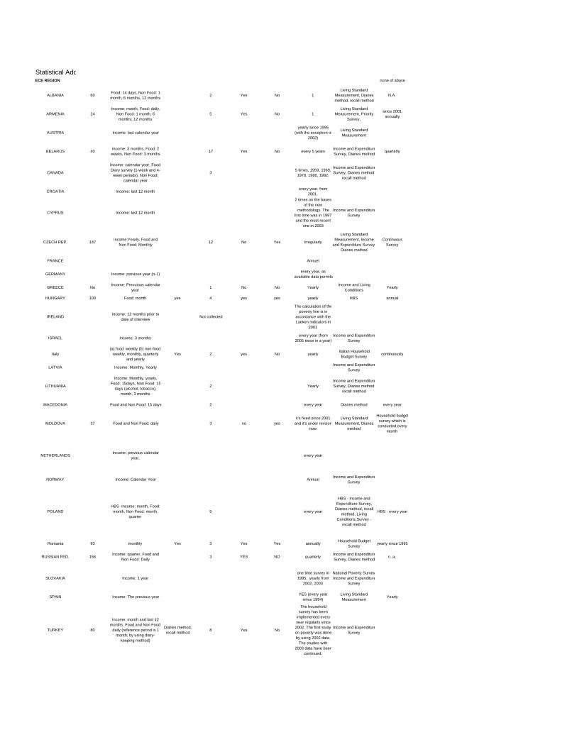
Statistical AddECE REGION
ALBANIA
ARMENIA
AUSTRIA
BELARUS
CANADA
CROATIA
CYPRUS
CZECH REP.
FRANCE
GERMANY
GREECE
HUNGARY
IRELAND
ISRAEL
Italy
LATVIA
LITHUANIA
MACEDONIA
MOLDOVA
NETHERLANDS
NORWAY
POLAND
Romania
RUSSIAN FED.
SLOVAKIA
SPAIN
TURKEY
none of above
60 Food: 14 days, Non Food: 1 month, 6 months, 12 months 2 Yes No 1
Living Standard Measurement, Diaries method, recall method
N.A.
24Income: month, Food: daily,
Non Food: 1 month, 6 months, 12 months
5 Yes No 1Living Standard
Measurement, Priority Survey,
since 2001 annually
Income: last calendar yearyearly since 1995
(with the exception of2002)
Living Standard Measurement
40 Income: 3 months, Food: 2 weeks, Non Food: 3 months 17 Yes No every 5 years Income and Expenditure
Survey, Diaries method quarterly
Income: calendar year, FoodDiary survey (1-week and 4-
week periods), Non Food: calendar year
3 5 times, 1959, 1969, 1978, 1986, 1992,
Income and ExpenditureSurvey, Diaries method,
recall method
Income: last 12 month every year, from 2001.
Income: last 12 month
2 times on the bases of the new
methodology. The first time was in 1997and the most recent
one in 2003
Income and ExpenditureSurvey
147 Income:Yearly, Food and Non Food: Monthly 12 No Yes Irregularly
Living Standard Measurement, Income
and Expenditure SurveyDiaries method
Continuous Survey
Annuel
Income: previous year (n-1) every year, as available data permits
No Income: Prevuious calendar year 1 No No Yearly Income and Living
Conditions Yearly
100 Food: month yes 4 yes yes yearly HBS annual
Income: 12 months prior to date of interview Not collected
The calculation of thepoverty line is in
accordance with the Laeken indicators in
2001
Income: 3 months every year (from 2005 twice in a year)
Income and ExpenditureSurvey
(a) food: weekly (b) non-foodweekly, monthly, quarterly
and yearlyYes 2 yes No yearly Italian Household
Budget Survey continuously
Income: Monthly, Yearly Income and ExpenditureSurvey
Income: Monthly, yearly, Food: 15days, Non Food: 15
days (alcohol, tobacco), month, 3 months
2 YearlyIncome and ExpenditureSurvey, Diaries method,
recall method
Food and Non Food: 15 days 2 every year Diaries method every year
37 Food and Non Food: daily 3 no yesit's fixed since 2001
and it's under revisonnow
Living Standard Measurement, Diaries
method
Household budgetsurvey which is conducted every
month
Income: previous calendar year, every year
Income: Calendar Year Annual Income and ExpenditureSurvey
HBS -Income: month, Food: month, Non Food: month,
quarter5 every year
HBS - Income and Expenditure Survey,
Diaries method, recall method, Living
Conditions Survey - recall method
HBS - every year
93 monthly Yes 3 Yes Yes annually Household Budget Survey yearly since 1995
156 Income: quarter, Food and Non Food: Daily 3 YES NO quarterly Income and Expenditure
Survey, Diaries method n. a.
Income: 1 yearone time survey in 1995, yearly from
2002, 2003
National Poverty SurveyIncome and Expenditure
Survey
Income: The previous year YES (every year since 1994)
Living Standard Measurement Yearly
80
Income: month and last 12 months, Food and Non Food
daily (reference period is 1 month; by using diary-
keeping method)
Diaries method, recall method 8 Yes No
The household survey has been
implemented every year regularly since
2002. The first study on poverty was doneby using 2002 data.
The studies with 2003 data have been
continued.
Income and ExpenditureSurvey
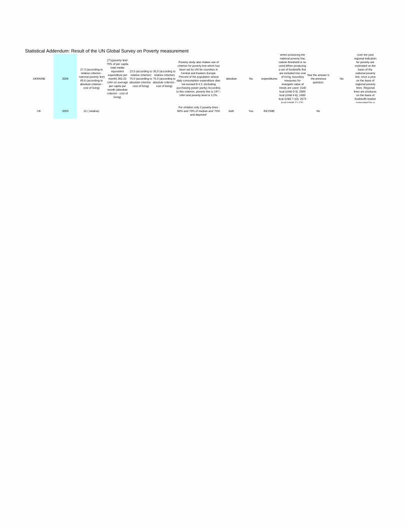
Statistical Addendum: Result of the UN Global Survey on Poverty measurement
UKRAINE 2004
27.3 (according to relative criterion -
national poverty line) 65.6 (according to absolute criterion -
cost of living)
271(poverty linel: 75% of per capita
total media equivalent
expenditure per month) 362.23
UAH on average per capita per
month (absolute criterion - cost of
living)
23.5 (according torelative criterion)
75.0 (according toabsolute criterion -
cost of living)
35,0 (according torelative criterion)
75.0 (according toabsolute criterion -
cost of living)
Poverty study also makes use of criterion for poverty line which has
been set by UN for countries in Central and Eastern Europe.
Percent of the population whose daily consumption expenditure does
not exceed $ 4.3. (including purchasing power parity) Accordingto this criterion, poverty line is 147.7
UAH and poverty level is 3.2%.
absolute No expenditures
When producing the national poverty line,
calorie threshold is notused.When producing a set of foodstuffs thatare included into cost
of living, boundary measures for
energetic value of meals are used: 1540 kcal (child 0-3); 2000 kcal (child 4-6); 2400
kcal (child 7-10); 2675kcal (child 11-13);
See the answer tothe previous
question. No
Over the year regional indicators
for poverty are estimated on the
basis of the national poverty line; once a year on the basis of regional poverty lines. Regional
lines are producedon the basis of
foodstuffs basket consumed by a
UK 2003 21 ( relative) For children only 3 poverty lines - 60% and 70% of median and '70%
and deprived'both Yes INCOME No
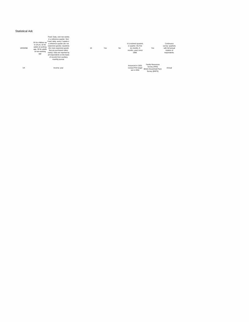
Statistical Add
UKRAINE
UK
55 for children up to 18 yrs, 42 for adults at working age, 39 for adults
at non-working age
Food: Daily, over two weeks in a reference quarter. Non
Food: daily, every 2 weeks ina reference quarter (for not expensive goods). Quarterly (for more expensive goods that are purchased rather
rarely). Data are reported by all respondents on the basis
of records from auxiliary monthly journal.
16 Yes No
It is estimed quarterly(1 quarter, the first
six months, 9 months, year) since
1999.
Yes
Continuous survey: quarterly with full annual
rotation of respondents.
Income: yearAnounced in 2003, revised PSA target
set in 2004
Family Resources Survey (FRS)
British Household PanelSurvey (BHPS)
Annual
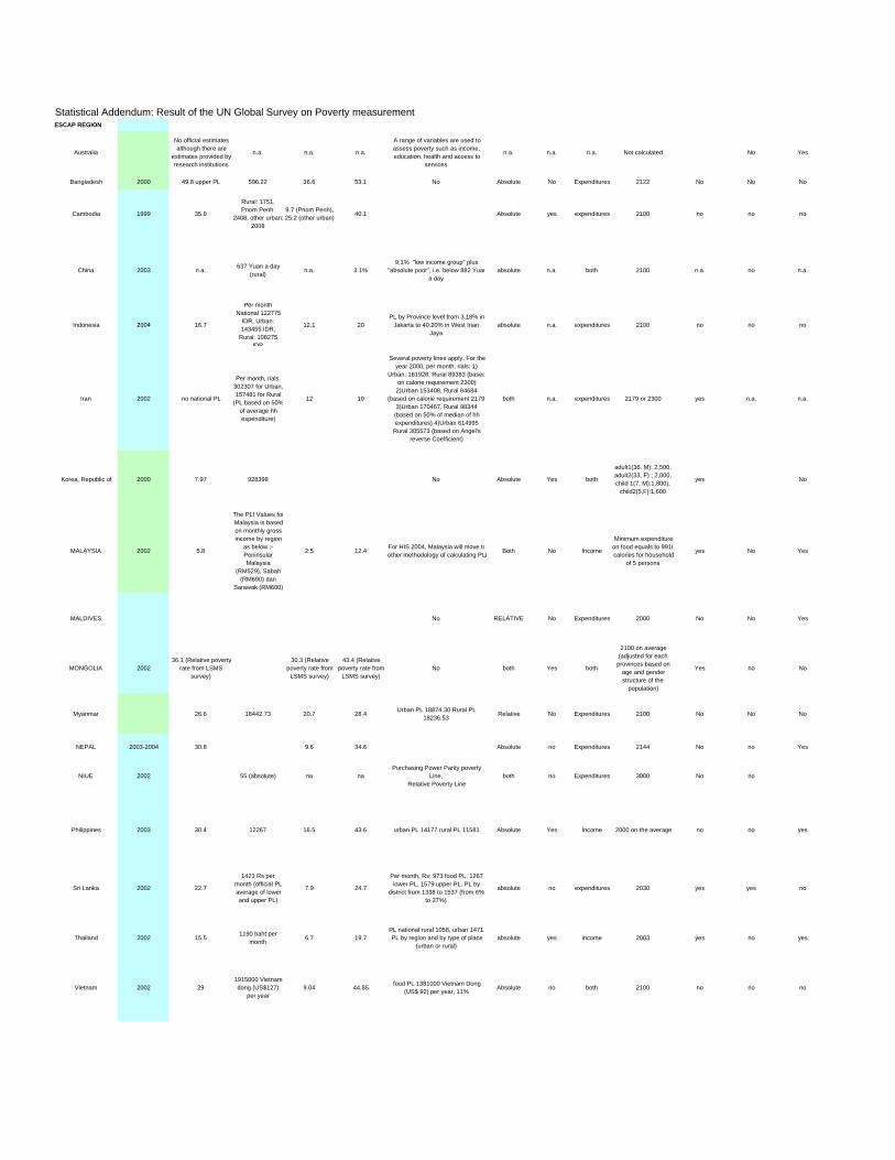
Statistical Addendum: Result of the UN Global Survey on Poverty measurementESCAP REGION
Australia
No official estimates although there are
estimates provided byresearch institutions
n.a. n.a. n.a.
A range of variables are used to assess poverty such as income, education, health and access to
services
n.a. n.a. n.a. Not calculated No Yes
Bangladesh 2000 49.8 upper PL 596.22 36.6 53.1 No Absolute No Expenditures 2122 No No No
Cambodia 1999 35.9
Rural: 1751, Pnom Penh:
2408, other urban:2008
9.7 (Pnom Penh), 25.2 (other urban) 40.1 Absolute yes expenditures 2100 no no no
China 2003 n.a. 637 Yuan a day (rural) n.a. 3.1%
9,1% "low income group" plus "absolute poor", i.e. below 882 Yuan
a dayabsolute n.a. both 2100 n.a. no n.a.
Indonesia 2004 16.7
Per month National 122775
IDR, Urban: 143455 IDR,
Rural: 108275 IDR
12.1 20PL by Province level from 3.18% in
Jakarta to 40.20% in West Irian Jaya
absolute n.a. expenditures 2100 no no no
Iran 2002 no national PL
Per month, rials. 302307 for Urban,157481 for Rural
(PL based on 50%of average hh expenditure)
12 10
Several poverty lines apply. For the year 2000, per month, rials: 1)
Urban: 161928, Rural 89383 (basedon calorie requirement 2300)
2)Urban 153408, Rural 84684 (based on calorie requirement 2179
3)Urban 170467, Rural 98344 (based on 50% of median of hh expenditures) 4)Urban 614995
Rural 305573 (based on Angel's reverse Coefficient)
both n.a. expenditures 2179 or 2300 yes n.a. n.a.
Korea, Republic of 2000 7.97 928398 No Absolute Yes both
adult1(36. M): 2,500, adult2(33, F) ; 2,000, child 1(7, M):1,800),
child2(5,F):1,600
yes No
MALAYSIA 2002 5.8
The PLI Values forMalaysia is basedon monthly gross income by region
as below :- Peninsular Malaysia
(RM529), Sabah (RM690) dan
Sarawak (RM600)
2.5 12.4 For HIS 2004, Malaysia will move toother methodology of calculating PLI Both No Income
Minimum expenditure on food equals to 9910calories for household
of 5 persons
yes No Yes
MALDIVES No RELATIVE No Expenditures 2000 No No Yes
MONGOLIA 200236.1 (Relative poverty
rate from LSMS survey)
30.3 (Relative poverty rate from
LSMS survey)
43.4 (Relative poverty rate from
LSMS survey)No both Yes both
2100 on average (adjusted for each
provinces based on age and gender structure of the
population)
Yes no No
Myanmar 26.6 18442.73 20.7 28.4 Urban PL 18874.30 Rural PL 18236.53 Relative No Expenditures 2100 No No No
NEPAL 2003-2004 30.8 9.6 34.6 Absolute no Expenditures 2144 No no Yes
NIUE 2002 55 (absolute) na naPurchasing Power Parity poverty
Line,Relative Poverty Line
both no Expenditures 3000 No no
Philippines 2003 30.4 12267 16.5 43.6 urban PL 14177 rural PL 11581 Absolute Yes Income 2000 on the average no no yes
Sri Lanka 2002 22.7
1423 Rs per month (official PL average of lower and upper PL)
7.9 24.7
Per month, Rs: 973 food PL, 1267 lower PL, 1579 upper PL. PL by
district from 1338 to 1537 (from 6% to 37%)
absolute no expenditures 2030 yes yes no
Thailand 2002 15.5 1190 baht per month 6.7 19.7
PL national rural 1058, urban 1471.PL by region and by type of place
(urban or rural)absolute yes income 2003 yes no yes
Vietnam 2002 291915000 Vietnam dong (US$127)
per year9.04 44.85 food PL 1381000 Vietnam Dong
(US$ 92) per year, 11% Absolute no both 2100 no no no
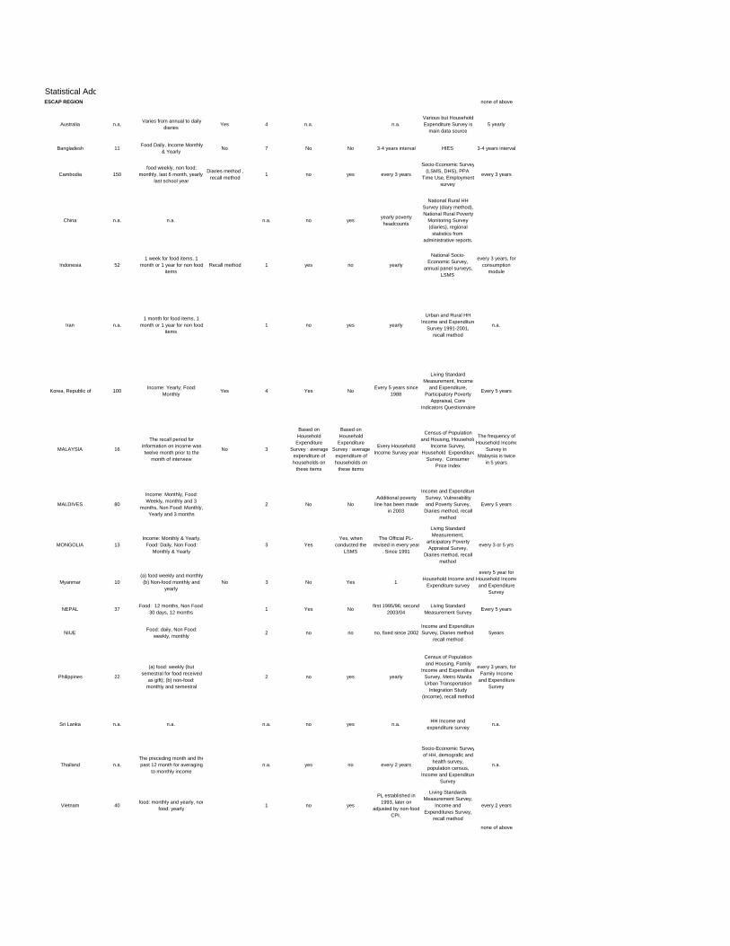
Statistical AddESCAP REGION
Australia
Bangladesh
Cambodia
China
Indonesia
Iran
Korea, Republic of
MALAYSIA
MALDIVES
MONGOLIA
Myanmar
NEPAL
NIUE
Philippines
Sri Lanka
Thailand
Vietnam
none of above
n.a. Varies from annual to daily diaries Yes 4 n.a. n.a.
Various but Household Expenditure Survey is
main data source5 yearly
11 Food Daily, Income Monthly & Yearly No 7 No No 3-4 years interval HIES 3-4 years interval
150food weekly, non food:
monthly, last 6 month, yearlylast school year
Diaries method , recall method 1 no yes every 3 years
Socio-Economic Survey(LSMS, DHS), PPA
Time Use, Employment survey
every 3 years
n.a. n.a. n.a. no yes yearly poverty headcounts
National Rural HH Survey (diary method), National Rural Poverty
Monitoring Survey (diaries), regional
statistics from administrative reports.
521 week for food items, 1
month or 1 year for non fooditems
Recall method 1 yes no yearly
National Socio-Economic Survey,
annual panel surveys, LSMS
every 3 years, for consumption
module
n.a.1 month for food items, 1
month or 1 year for non fooditems
1 no yes yearly
Urban and Rural HH Income and Expenditure
Survey 1991-2001, recall method
n.a.
100 Income: Yearly; Food: Monthly Yes 4 Yes No Every 5 years since
1988
Living Standard Measurement, Income
and Expenditure, Participatory Poverty
Appraisal, Core Indicators Questionnaire
Every 5 years
16
The recall period for information on income was twelve month prior to the
month of interview
No 3
Based on Household
Expenditure Survey : average
expenditure of households on
these items
Based on Household
Expenditure Survey : average
expenditure of households on
these items
Every Household Income Survey year
Census of Population and Housing, Household
Income Survey, Household Expenditure
Survey, Consumer Price Index
The frequency of Household Income
Survey in Malaysia is twice
in 5 years
80
Income: Monthly, Food: Weekly, monthly and 3
months, Non Food: Monthly,Yearly and 3 months
2 No NoAdditional poverty
line has been made in 2003
Income and ExpenditureSurvey, Vulnerability and Poverty Survey,
Diaries method, recall method
Every 5 years
13Income: Monthly & Yearly,
Food: Daily, Non Food: Monthly & Yearly
3 YesYes, when
conducted the LSMS
The Official PL- revised in every year
. Since 1991
Living Standard Measurement,
articipatory Poverty Appraisal Survey,
Diaries method, recall method
every 3 or 5 yrs
10(a) food weekly and monthly (b) Non-food monthly and
yearlyNo 3 No Yes 1 Household Income and
Expenditure survey
every 5 year for Household Incomeand Expenditure
Survey
37 Food: 12 months, Non Food30 days, 12 months 1 Yes No first 1995/96; second
2003/04Living Standard
Measurement Survey Every 5 years
Food: daily, Non Food: weekly, monthly 2 no no no, fixed since 2002
Income and ExpenditureSurvey, Diaries method,
recall method5years
22
(a) food: weekly (but semestral for food received
as gift); (b) non-food: monthly and semestral
2 no yes yearly
Census of Population and Housing, Family
Income and ExpenditureSurvey, Metro Manila Urban Transportation
Integration Study (income), recall method
every 3 years, for Family Income
and Expenditure Survey
n.a. n.a. n.a. no yes n.a. HH Income and expenditure survey n.a.
n.a.The preceding month and thepast 12 month for averaging
to monthly incomen.a. yes no every 2 years
Socio-Economic Surveyof HH, demografic and
health survey, population census,
Income and ExpenditureSurvey
n.a.
40 food: monthly and yearly, nonfood: yearly 1 no yes
PL established in 1993, later on
adjusted by non-foodCPI.
Living Standards Measurement Survey,
Income and Expenditures Survey,
recall method
every 2 years
none of above
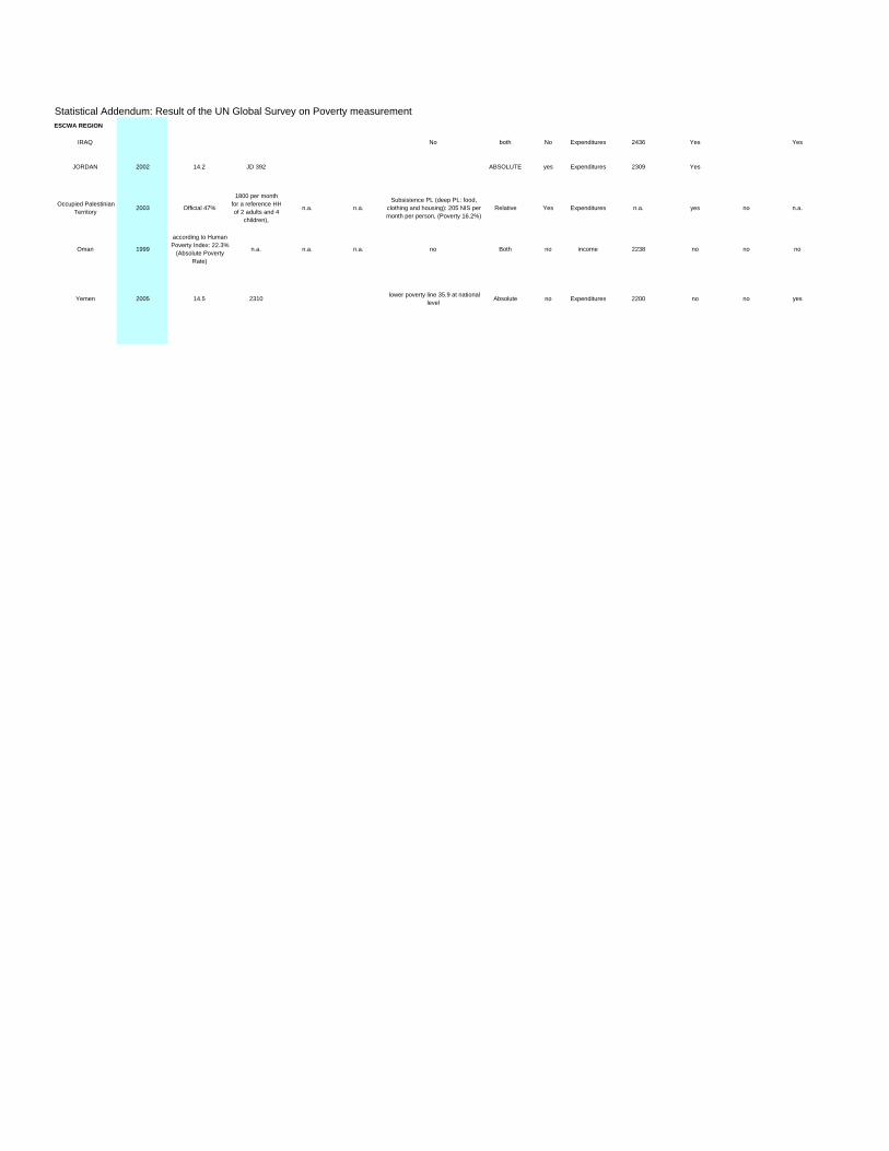
Statistical Addendum: Result of the UN Global Survey on Poverty measurementESCWA REGION
IRAQ No both No Expenditures 2436 Yes Yes
JORDAN 2002 14.2 JD 392 ABSOLUTE yes Expenditures 2309 Yes
Occupied Palestinian Territory 2003 Official 47%
1800 per month for a reference HHof 2 adults and 4
children),
n.a. n.a.Subsistence PL (deep PL: food,
clothing and housing): 205 NIS per month per person, (Poverty 16.2%)
Relative Yes Expenditures n.a. yes no n.a.
Oman 1999
according to Human Poverty Index: 22.3%
(Absolute Poverty Rate)
n.a. n.a. n.a. no Both no income 2238 no no no
Yemen 2005 14.5 2310 lower poverty line 35.9 at national level Absolute no Expenditures 2200 no no yes
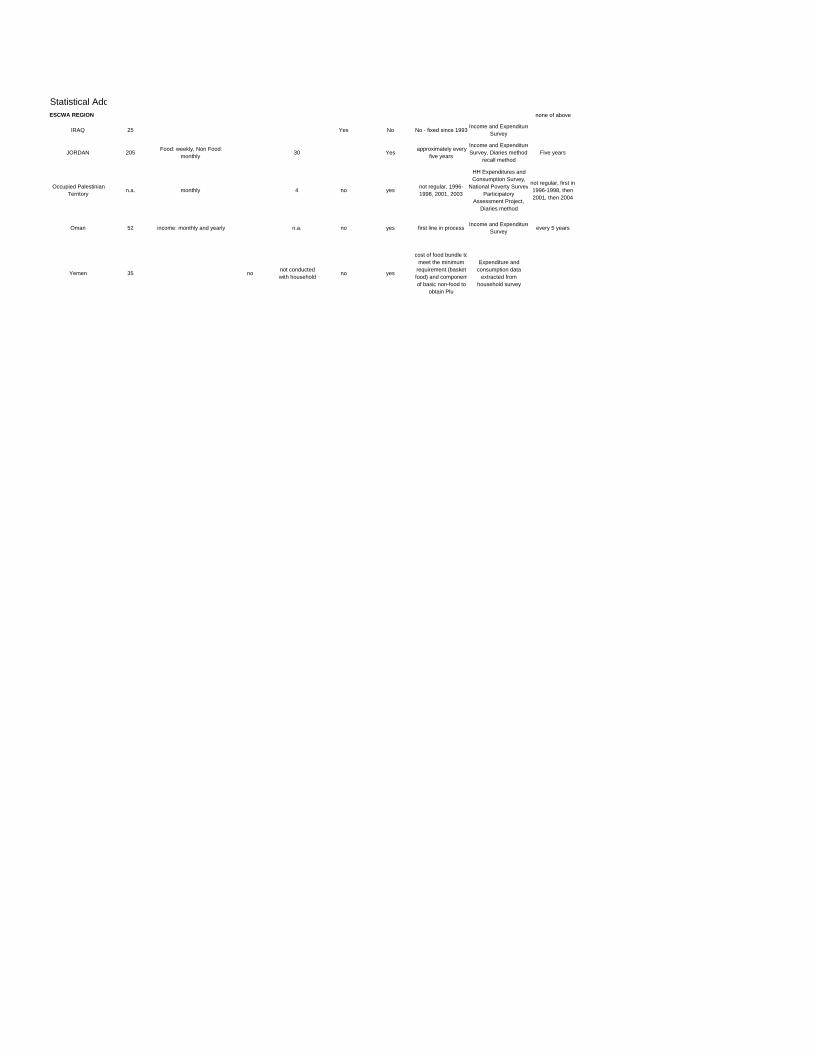
Statistical AddESCWA REGION
IRAQ
JORDAN
Occupied Palestinian Territory
Oman
Yemen
none of above
25 Yes No No - fixed since 1993 Income and ExpenditureSurvey
205 Food: weekly, Non Food: monthly 30 Yes approximately every
five years
Income and ExpenditureSurvey, Diaries method,
recall methodFive years
n.a. monthly 4 no yes not regular, 1996-1998, 2001, 2003
HH Expenditures and Consumption Survey,
National Poverty SurveyParticipatory
Assessment Project, Diaries method
not regular, first in1996-1998, then 2001, then 2004
52 income: monthly and yearly n.a. no yes first line in process Income and ExpenditureSurvey every 5 years
35 no not conducted with household no yes
cost of food bundle tomeet the minimum
requirement (basket food) and componentof basic non-food to
obtain Plu
Expenditure and consumption data
extracted from household survey