Contents

Introduction 1

Why Read this Handbook? . . . . . . . . . . . . . . . . . . . . . . 1

How to Use this Handbook . . . . . . . . . . . . . . . . . . . . . . 2

Course Structure 3

The Audience . . . . . . . . . . . . . . . . . . . . . . . . . . . . . . 3

The Starting Points . . . . . . . . . . . . . . . . . . . . . . . . . . 4

Curricular Themes . . . . . . . . . . . . . . . . . . . . . . . . . . . 5

Context . . . . . . . . . . . . . . . . . . . . . . . . . . . . . . 5

Differential Equations . . . . . . . . . . . . . . . . . . . . . . 6

Modelling . . . . . . . . . . . . . . . . . . . . . . . . . . . . . 7

Successive Approximations . . . . . . . . . . . . . . . . . . . 7

Geometric Visualization . . . . . . . . . . . . . . . . . . . . . 7

Numerical Methods . . . . . . . . . . . . . . . . . . . . . . . . 8

Pedagogical Aspects . . . . . . . . . . . . . . . . . . . . . . . . . . 8

Collaboration . . . . . . . . . . . . . . . . . . . . . . . . . . . 8

Calculus as a Language . . . . . . . . . . . . . . . . . . . . . 9

Tackling Large, Messy, Ill-Defined Problems . . . . . . . . . . 9

Experimentation . . . . . . . . . . . . . . . . . . . . . . . . . 10

Approximation . . . . . . . . . . . . . . . . . . . . . . . . . . 10

The Importance of Problems . . . . . . . . . . . . . . . . . . 10

The Role of the Text . . . . . . . . . . . . . . . . . . . . . . . 11

Intuition and Rigor . . . . . . . . . . . . . . . . . . . . . . . . 12

Rethinking Techniques . . . . . . . . . . . . . . . . . . . . . . 12

Example 1: Maxima-minima . . . . . . . . . . . . . . 13

Example 2: Differential equations . . . . . . . . . . . . 14

Computing . . . . . . . . . . . . . . . . . . . . . . . . . . . . . . . 14

Classroom Layout . . . . . . . . . . . . . . . . . . . . . . . . 14

i

ii CONTENTS

Computer Labs . . . . . . . . . . . . . . . . . . . . . . . . . . 15Appropriate Use of Technology . . . . . . . . . . . . . . . . . 15

Software vs. programming . . . . . . . . . . . . . . . . . . . . 16Calculators vs. computers . . . . . . . . . . . . . . . . . . . . 17

Support . . . . . . . . . . . . . . . . . . . . . . . . . . . . . . 18Handouts . . . . . . . . . . . . . . . . . . . . . . . . . 18

Prompt answers . . . . . . . . . . . . . . . . . . . . . 18Traps for the Unwary . . . . . . . . . . . . . . . . . . . . . . 19

Roundoff error . . . . . . . . . . . . . . . . . . . . . . 19Overflow . . . . . . . . . . . . . . . . . . . . . . . . . . 20

Misleading results . . . . . . . . . . . . . . . . . . . . 20Time Demands . . . . . . . . . . . . . . . . . . . . . . . . . . . . . 21

Time Demands on the Teacher . . . . . . . . . . . . . . . . . 22Time Demands on the Student . . . . . . . . . . . . . . . . . 23

Testing and Evaluation . . . . . . . . . . . . . . . . . . . . . . . . 24

Chapter-by-Chapter Commentary 27

Chapter 1. A Context for Calculus . . . . . . . . . . . . . . . . . . 27

1.1 The Spread of Disease . . . . . . . . . . . . . . . . . . . . 271.2 The Mathematical Ideas . . . . . . . . . . . . . . . . . . . 30

1.3 Using a Computer (or Graphing Calculator) . . . . . . . . 30Some Historical Notes on the S-I-R Model . . . . . . . . . . 30

Further Reading . . . . . . . . . . . . . . . . . . . . . . . . . 31Chapter 2. Successive Approximations . . . . . . . . . . . . . . . . 32

2.1 Making Approximations . . . . . . . . . . . . . . . . . . . 322.2 Euler’s Method . . . . . . . . . . . . . . . . . . . . . . . . 34

2.3 Approximate Solutions . . . . . . . . . . . . . . . . . . . . 34Chapter 3. The Derivative . . . . . . . . . . . . . . . . . . . . . . . 35

3.1 Rates of Change . . . . . . . . . . . . . . . . . . . . . . . 363.2 Microscopes and Local Linearity . . . . . . . . . . . . . . 37

3.3 The Derivative . . . . . . . . . . . . . . . . . . . . . . . . 383.4 Estimation and Error Analysis . . . . . . . . . . . . . . . 39

3.5 A Global View . . . . . . . . . . . . . . . . . . . . . . . . 393.6 The Chain Rule . . . . . . . . . . . . . . . . . . . . . . . . 40

3.7 Partial Derivatives . . . . . . . . . . . . . . . . . . . . . . 41Chapter 4. Differential Equations . . . . . . . . . . . . . . . . . . . 41

4.1 Modelling with Differential Equations . . . . . . . . . . . 414.2 Solutions of Differential Equations . . . . . . . . . . . . . 42

4.3 The Exponential Function . . . . . . . . . . . . . . . . . . 43

CONTENTS iii

4.4 The Logarithm Function . . . . . . . . . . . . . . . . . . . 444.5 The Equation y′ = f(t) . . . . . . . . . . . . . . . . . . . 45Further Reading . . . . . . . . . . . . . . . . . . . . . . . . . 45

Chapter 5. Techniques of Differentiation . . . . . . . . . . . . . . . 465.1 The Differentiation Rules . . . . . . . . . . . . . . . . . . 465.2 Finding Partial Derivatives . . . . . . . . . . . . . . . . . 465.3 The Shape of the Graph of a Function . . . . . . . . . . . 475.4 Optimal Shapes . . . . . . . . . . . . . . . . . . . . . . . . 475.5 Newton’s Method . . . . . . . . . . . . . . . . . . . . . . . 47

Chapter 6. The Integral . . . . . . . . . . . . . . . . . . . . . . . . 486.1 Measuring Work . . . . . . . . . . . . . . . . . . . . . . . 486.2 Riemann Sums . . . . . . . . . . . . . . . . . . . . . . . . 486.3 The Integral . . . . . . . . . . . . . . . . . . . . . . . . . . 496.4 The Fundamental Theorem . . . . . . . . . . . . . . . . . 49

Chapter 7. Periodicity . . . . . . . . . . . . . . . . . . . . . . . . . 497.1 Periodic Behavior . . . . . . . . . . . . . . . . . . . . . . . 507.2 Period, Frequency, and the Circular Functions . . . . . . . 507.3 Differential Equations with Periodic Solutions . . . . . . . 51Further Reading . . . . . . . . . . . . . . . . . . . . . . . . . 51

Chapter 8. Dynamical Systems . . . . . . . . . . . . . . . . . . . . 528.1 State Spaces and Vector Fields . . . . . . . . . . . . . . . 528.2 Local Behavior of Dynamical Systems . . . . . . . . . . . 538.3 A Taxonomy of Equilibrium Points . . . . . . . . . . . . . 538.4 Limit Cycles . . . . . . . . . . . . . . . . . . . . . . . . . 538.5 Beyond the Plane:Three-Dimensional Systems . . . . . . . 54Further Reading . . . . . . . . . . . . . . . . . . . . . . . . . 54

Chapter 9. Functions of Several Variables . . . . . . . . . . . . . . 559.1 Graphs and Level Sets . . . . . . . . . . . . . . . . . . . . 559.2 Local Linearity . . . . . . . . . . . . . . . . . . . . . . . . 569.3 Optimization . . . . . . . . . . . . . . . . . . . . . . . . . 57

Chapter 10. Series and Approximations . . . . . . . . . . . . . . . 5710.1 Approximation at a Point and Over an Interval . . . . . 5710.2 Taylor Polynomials . . . . . . . . . . . . . . . . . . . . . 5810.3 Taylor Series . . . . . . . . . . . . . . . . . . . . . . . . . 5810.4 Power Series and Differential Equations . . . . . . . . . . 5810.5 Convergence . . . . . . . . . . . . . . . . . . . . . . . . . 5910.6 Approximation Over Intervals . . . . . . . . . . . . . . . 59Further Reading . . . . . . . . . . . . . . . . . . . . . . . . . 59

Chapter 11. Techniques of Integration . . . . . . . . . . . . . . . . 59

iv CONTENTS

11.1 Antiderivatives . . . . . . . . . . . . . . . . . . . . . . . 6111.2 Integration by Substitution . . . . . . . . . . . . . . . . . 6111.3 Integration by Parts . . . . . . . . . . . . . . . . . . . . 6111.4 Separation of Variables and Partial Fractions . . . . . . 6211.5 Trigonometric Integrals . . . . . . . . . . . . . . . . . . . 6211.6 Simpson’s Rule . . . . . . . . . . . . . . . . . . . . . . . 6211.7 Improper Integrals . . . . . . . . . . . . . . . . . . . . . 62

Chapter 12. Case Studies . . . . . . . . . . . . . . . . . . . . . . . 6312.1 Stirling’s Formula . . . . . . . . . . . . . . . . . . . . . . 6312.2 The Poisson Distribution . . . . . . . . . . . . . . . . . . 6412.3 The Power Spectrum . . . . . . . . . . . . . . . . . . . . 64Further Reading . . . . . . . . . . . . . . . . . . . . . . . . . 6512.4 Fourier Series . . . . . . . . . . . . . . . . . . . . . . . . 66

Appendix A: Sample Syllabi 67

Calculus I Syllabus . . . . . . . . . . . . . . . . . . . . . . . . . . . 69Calculus II Syllabus . . . . . . . . . . . . . . . . . . . . . . . . . . 71

Appendix B: Sample Exams and Quizzes 73

Appendix C: Drill Sheets 105

Appendix D: Supplementary Laboratory Exercises 121

Appendix E: Supplementary Programs 133

Appendix F: Solutions 143

Introduction

In the summer of 1988 a group of us from the Five Colleges—Amherst,Hampshire, Mount Holyoke, and Smith Colleges, and the University ofMassachusetts—in western Massachusetts began working on a new calculuscurriculum under a five-year grant from the National Science Foundation.We had two broad goals in mind: 1) to develop the concepts of calculus inthe context of substantial problems from the other sciences, and 2) to incor-porate the visual and computational power of computers into the explorationof these concepts.

For the first five years, at the end of each semester the faculty who hadtaught the material got together for a daylong session to share experiencesof what had worked well and what difficulties had been encountered. Eachsummer we then worked to revise the materials and write new sections, iron-ing out those spots that had been unclear or where the purity of our initialconception ran into the realities of the classroom. We also ran a number ofworkshops around the country for other faculty thinking of using the mate-rials. This Handbook is a distillation of the topics and issues which regularlyarose during the debriefing sessions and workshops. As more teachers usethese materials in a wider range of settings, the Handbook will undoubtedlycontinue to be revised. We would therefore like very much to hear from youabout things that didn’t work for you, pitfalls or opportunities that devel-oped in your class, or about suggested improvements in either the text orthis Handbook.

Why Read this Handbook?

There are a number of snares lying in wait for those teaching this material forthe first time. The choice, order, and development of topics are substantiallydifferent from the way most of us were taught, and have ourselves been

1

2 INTRODUCTION

teaching. This provides many points at which new users of these materialscan anticipate how they think the material will or should unfold, only to beleft off-balance when a very different tack is taken. In this Handbook we flaga number of these points and explain the choices made.

Moreover, this course in places draws upon examples from domains likeepidemiology or ecology that are not part of the standard training of mostmathematics teachers. While the examples are meant to be self-contained,a number of teachers have expressed an interest in having more of the back-ground available. This Handbook therefore includes supplemental discussionand references for those wishing to explore the topics further.

Finally, this course is technology-dependent to a much greater extentthan the courses many of us are used to teaching. We identify a numberof technical and pedagogical issues that have come up relating to the use ofcomputers or graphing calculators, and include some suggestions for dealingwith them.

How to Use this Handbook

The body of the Handbook consists of two main sections. The first 25 pageson Course Structure lay out the general pedagogical and curricular concernsunderlying the choice and presentation of topics, with some suggestions re-garding their implementation. The remainder of the body of the Handbook

is a section-by-section commentary on the text.Throughout, this Handbook and the main text should be viewed as a

guide only. The arrangement of the topics in the text is a suggestion, anorder which has worked well for us. Even we don’t go through every item inorder every time. You undoubtedly have your own pet examples and waysof covering some topics, and you should certainly feel free to customize thematerials. Nevertheless, if you are trying the material for the first time, weurge you to stay fairly close to the order and style given to get a good overallfeel for the novel features of this approach. For purposes of future versionsof the text and this Handbook , if you do try a variation which works well,please let us know.

Course Structure

The Audience

The original users of these materials were undergraduates at four-year liberalarts colleges, majoring in everything from mathematics to the arts. Byand large, they are not unusually gifted mathematically and have as muchdifficulty as most undergraduates in remembering the quadratic formula.When we began, we thought a separate course for mathematics and physicsmajors might be needed, but we have come to feel that this course’s view ofmathematics and its relation to the other disciplines is an important one forthese students to cultivate as well, and we now have them all in one course.Now, many students at high schools, two-year colleges, and universities arealso using this text.

As is increasingly the case at a number of schools, many of our studentsarrive having already completed a calculus course elsewhere, and the usualproblems of deciding where to place them arise. For those whose backgroundis quite strong, we have found that they can generally acquire the ideas andtools of this course in their other work, without taking this course. Forthose not quite this strong, moving directly into the second semester materialworks well, requiring only a bit of scrambling on their part at the beginningof the term to become familiar with some of the numerical concepts involved.

The less strong students who have had calculus before, though, or thoselooking for an easy course (since they think they already know the mate-rial), pose particular problems. These students usually sign up for the firstsemester. For most of them, this works out well—the material is differentenough from what they’ve seen so they don’t get bored, and the new per-spective often helps them understand the concepts more profoundly. Some,though, feel betrayed when they see how different this course is from whatthey’ve had before, responding with “When are we going to get to the cal-culus?” and resenting the time they have to put into the course when they

3

4 COURSE STRUCTURE

thought they knew it already. It helps to point out the kinds of problemsthey are able to solve in this course that they couldn’t have dealt with intheir previous course.

As always in launching something new in the classroom, it is importantto make sure the students see themselves as our co-experimenters rather thanas our guinea pigs. As they compare this course with their own experiencesor with other courses their friends are taking, they will need reassurance thatwe know what we are doing. We have found that one of the most helpfulthings we as teachers can do is to talk to our students—explain what we aredoing and why; tell them how this course compares with a more traditionalcourse, without belittling the standard course; get feedback early and often.The issues can’t be adequately addressed in a single conversation at thebeginning of the semester, but need to recur throughout the course, moreoften than our initial intuitions would have suggested.

The Starting Points

The material in this course is based on five premises:

1. Calculus is fundamentally a way of dealing with functional relation-ships that occur in scientific contexts. The language, tools, and modelsof calculus arose through trying to understand these relationships, andthe other sciences still provide an ongoing source of new and interest-ing topics for investigation. An awareness of this connection should bea part of the students’ perception of the material from the beginning.Particularly in the initial stages, developing the techniques of calcu-lus must not obscure an overview of the kinds of underlying questionscalculus is designed to explore.

2. Computers radically enlarge the range of questions we can explore andthe ways we can address them. Computers are much more than atool for teaching standard calculus; they change the standard. Whenwe can replace sophisticated analytical techniques with conceptuallysimple computational approaches, some important classes of problemsthat were formerly considered to be advanced can now be explored atthe introductory level. Moreover, numerical approaches often providea generality in the treatment of topics like integration and differen-tial equations which, in the traditional exposition, can appear to be amiscellany of special cases. Finally, computers encourage a geometric

CURRICULAR THEMES 5

approach which can substantially enhance the students’ mathematicalunderstanding.

3. The concept of a dynamical system is central to science, as any perusalof the current literature will quickly indicate. Therefore, calculus mustprepare students, preferably at an early stage, to begin dealing withsystems of non-linear differential equations and the kinds of questionsthat arise about such systems.

4. The concept of derivative is much more fundamental than, and is sep-arable from, the process of differentiation. It has been our experiencein the past that students all too often think of the derivative only interms of a set of differentiation rules. In fact, in many contexts—dynamical systems, for instance—the derivative is given by a modelor by a geometric analysis rather than from differentiating some func-tion. Students need a clear geometric and operational understandingof what a derivative is in its own right.

5. The process of successive approximation is a key tool of calculus, evenwhen the outcome of the process—the limit—cannot be explicitly givenin closed form. The standard ε–δ approach, assuming as it does that wesomehow know the answer, is often a much less useful way of thinkingabout the limiting process than Cauchy’s approach.

Curricular Themes

We have taken the above starting points and abstracted a small set of themesfrom them, around which we have organized the curriculum.

Context

If you ask typical students what mathematics is about, they are likely todeny that it is about anything. They perceive mathematics as existing in aworld of its own, with its own rules, having little to do with any questionsthey might be interested in. The so-called “applications” that are provided,almost always after the mathematics has been completely worked out, areoften transparently artificial and do little to convince skeptical students thatmathematics has anything to say about the world in which they live. Wefeel much of the low regard the general public currently has for mathematics

6 COURSE STRUCTURE

arises from treating mathematics as a strictly technical discipline, responsiveonly to its own internal logic and structure.

Historically, though, much of calculus arose as a tool to explore questionsin the sciences—including, of course, other branches of mathematics. Ourstudents need to see this connection throughout as they learn the material,not just as an optional afterthought appended to the mathematics.

Providing this kind of context for the mathematical ideas can be dauntingfor many teachers. Few of us have the training to claim expertise in any fieldoutside mathematics, and none of us has the time to acquire such expertisenow. The main advice is: Don’t try to present yourself as an expert. If youare in command of the mathematical component, students can readily acceptyour role is an intelligent amateur in ecology, physics, or chemistry. Theywill even enjoy the role reversal, when they know more than you. While theexamples in the text are meant to be self-contained, some teachers will wantto develop their own examples. Your students can help in this, both duringthe course and after. They will be glad to enlarge your repertoire by bringingyou examples they come across where calculus is used. Your colleagues inthe other sciences can be good sources of examples and topics, and theywill appreciate being consulted. If you have the time and the inclination,skimming through journals like Science, Nature, or The American Naturalist

can suggest possible topics. This Handbook contains a modest selection ofsuggested readings which you can peruse if you are so inclined. View this asa long-term development, not as something which has to be accomplishedbefore you teach this material for the first time.

Differential Equations

In looking through the scientific journals, the large majority of settings inwhich calculus occurs take the following form: the investigators have a sys-tem of interacting quantities whose behavior they want to analyze, and theconstraints acting on the system allow them to model the rates at whichthe quantities are changing. That is, they start with a system of differen-tial equations, typically non-linear, and they want to know something aboutits solution curves, asymptotic behavior, or the existence and nature of anyequilibrium points.

Since this is such a universal feature of all the sciences, we have madeit a central theme of this course. This topic is introduced on page 1, in amodel for the progression of an epidemic, and is developed in many of thelater chapters.

CURRICULAR THEMES 7

Modelling

While we do not view this as a modelling course, it is important for studentsto develop a reasonably sophisticated appreciation for the interplay betweenreal-world problems and the mathematical models we construct to help usthink about these problems. A first difficulty in this process for many ofour students is simply one of translation—from descriptions expressed inEnglish to mathematical equations, and vice versa. Once students beginto be comfortable with this translation process it is possible to go on todiscuss issues like what makes for a good model, the value and place ofboth quantitative and qualitative prediction, and the like. In particular, itis useful for students to begin to develop a good feel for the role parametersplay in constructing models.

Successive Approximations

Up to this point in their mathematical education, every problem our studentshave encountered has had one correct answer. In this course, though, thisrarely happens. Solutions can be approximated to high degrees of accuracy,but the solution itself can not be written down in closed form. Thus theapproximations are not just useful clues leading up to the “real” answer like2 or π or sinx—often the approximations are all we have. This is a startlingshift for many students to make, and an important one. Moreover, studentsneed to develop a strong appreciation of the tradeoff in time (and perhapsmoney) in getting the next decimal place of accuracy in an approximation.

Geometric Visualization

A computer’s ability to produce and manipulate graphical images introducesa conceptual element that is very helpful in thinking about mathematicalproblems. We have tried to incorporate this into our course wherever wecould, encouraging our students to cultivate their geometric intuitions andto see calculus as more than a collection of algebraic rules for manipulatingstrings of symbols. When students can actually see the graph of a functionbecoming linear as they zoom in on it, or when they can see a series ofpiecewise-linear curves approaching a smooth curve as a limit, these conceptsbecome very real and concrete in ways that are difficult to achieve throughmore formal arguments.

8 COURSE STRUCTURE

Numerical Methods

Traditionally, numerical methods have been the last recourse, to be usedwhen one could think of no clever technique for producing a closed-formsolution to a problem. Students were implicitly taught to expect that mostproblems would be tractable, that only if they were really unlucky wouldthey have to resort to Simpson’s rule or Runge-Kutte techniques. Withreadily available computers, though, the position is reversed—students canbe taught to approach every problem of integration, for instance, knowingin advance that it is solvable by numerical methods at least, and that ifthey are really lucky it might even yield to a clever analytical shortcut likeintegration by parts. We feel that this shift in attitude is an important one,making our students more effective users of calculus since the concepts areseen in a more universal light.

At the same time, though, it is important to stress that this is not a coursein numerical techniques, and we often stay with a particular approach—Euler’s method, for instance—because of its conceptual simplicity, eventhough there may be other techniques that give more rapid convergence.

Pedagogical Aspects

In addition to these curricular themes, we have designed this course to en-courage our students to think about what it means to do mathematics inseveral ways which are new to many of them.

Collaboration

A great deal has been written about the role of collaborative learning, whichwe won’t go into here. In our calculus classes the students are stronglyencouraged to work in groups of two or three on the homework problems, andwe have found this to be very effective. The students encourage one anotherand work productively to make suggestions and try out possibilities that theywould not have had the confidence or energy for if working individually. Infact, many of the problems are so involved that it would be discouraging anddifficult for a typical student to work on them alone.

This immediately raises a number of questions for teachers: Do we assignstudents to groups or let them choose their own? How do we assign creditfor the work done? Do the groups turn in one solution set per group? Howdo we get shyer students into groups? While each teacher develops his or her

PEDAGOGICAL ASPECTS 9

own response to such questions, we have found none of them to be a majorhurdle. Some of us ask students to submit a single, joint homework paperrepresenting their group work. We try to be sure that the responsibility forwriting up joint solutions is shared evenly (for example, by asking studentsnot only to list all members of the group but also to indicate who wroteup each portion). Having regularly scheduled problem sessions outside ofclass is another good way to encourage students to work together. Havinga student assistant on hand at these sessions is helpful, too, so long as theassistant has been trained not to fall into the trap of being too helpful.

Calculus as a Language

For many people—both teachers and students—the most striking feature ofthe text is the number of words. Students used to a largely algebraic ap-proach to mathematics will be wondering where the formulas and equationsare. Moreover, the lack of “template” examples in the text that studentscan turn to and readily adapt for doing their homework forces many of themto revise the successful strategies they have evolved for dealing with mathe-matics courses.

The text is designed to remind students that mathematics problems ariseout of real world contexts and to give them ample practice in the art oftranslating such problems into mathematics. We believe that this transla-tion process from words to mathematics is an important part of being aneffective user of mathematics. The real problems that our students will en-counter outside our classes rarely come labeled and broken down into tidyparts. While they need to be proficient in the routine manipulations, stu-dents need to realize that there is more to being good at mathematics thanproficiency in manipulating symbols. We have found in previous courses thatthe ability to successfully perform mathematical manipulations does not al-ways coincide with the ability to assign meaning to such manipulations—tothink mathematically. We want our students to be fluent in moving backand forth between English statements and mathematical ones, and havestructured the text to reinforce this.

Tackling Large, Messy, Ill-Defined Problems

Once students leave their mathematics classes, they will often encounterproblems that don’t immediately suggest a specific technique for their solu-tion. There may be incomplete or irrelevant information, there will be too

10 COURSE STRUCTURE

many complexities to deal with all at once, and the like. We feel it is im-portant for our students to begin getting some practice with how they canmake a start in such a situation. We have therefore included a number ofproblems that require simplification or are first explored by generating dataand looking for patterns. We also ask students to think and write aboutwhat they are doing, articulating the pros and cons of various approaches.

Experimentation

An important part of thinking about hard problems is trying things out andexperimenting with different possibilities to see what happens. As othershave pointed out, computers can provide an experimental flavor to mathe-matics for the average student. One of the most striking features of teachingthis material in a computer classroom is how quickly the students escapethe control of the teacher. They try different models of a problem, varyparameters to see what patterns emerge, and exchange discoveries with oneanother. Having a setting where students can discover some of the truth forthemselves rather than simply having it handed on by the teacher is verypowerful.

Approximation

Thinking in terms of initial, approximate answers to a problem rather thanleaping immediately to the right answer is very difficult for many students,yet it is an attitude they must develop if they are ever to be able to approachlarge, messy problems with confidence. Making approximations also forcesstudents to think about the structure of a problem in ways they can oftenavoid if all they have to do is perform certain manipulations to get the rightanswer. The notion of approximation is central to most of the topics in thistext, and by the end students have a much more sophisticated conception ofthe role of approximations and how to use them intelligently.

The Importance of Problems

Most students come to this course with the general notion that mathematicsis about learning concepts and tools, and that doing problems—often ex-ercises, really—is where they get good at using the tools, which will thenbe tested on the exams. This course is structured to make wrestling withproblems much more central. We want the students to feel that they arelearning the tools so they can think about interesting problems, rather than

PEDAGOGICAL ASPECTS 11

that they are doing problems so they can learn the tools. While there is aplace for exercises that are moderately repetitive variations on a commontheme to help develop facility with a certain tool or concept, the skill ourstudents will need in the long run is to feel comfortable jumping into a prob-lem when it is not obvious what the appropriate approach is. Many of ourproblems are designed to develop this attitude.

Moreover, many problems anticipate ideas and directions that will nothave been covered yet in class, to get the students thinking about the issuesbefore they are raised by the teacher. This is a significant change in whatthe students are used to, and it helps if the teacher discusses the reasons forthis with the students.

There are several mechanisms we use for getting the students to take thehomework problems more seriously. One is simply to insist on more clarity inthe written explanations accompanying their answers. Another is to assignmore credit to the homework in computing the final grade—some of us countthe homework for as much as 50% of the grade. One arrangement we usethat helps the students’ learning is to permit students to resubmit homeworkpapers. It is helpful to have the original work attached to the revision so thereader can easily compare the two versions. A useful grading scheme is toassign one of three overall grades to each paper, for example 1, 2, or 3. Wemight tell students that “1” indicates they should get help and then re-dothe assignment (or those portions presenting difficulties); “2” indicates thatthey would benefit from re-doing the assignment; and “3” that the paperis good enough to study from. In practice this tends to mean that almostall groups end up with the grade of “3” on nearly all assignments, but thisseems fine to us.

The Role of the Text

As working on the problems becomes more central, students will need tolearn to use the text in ways that may be different from their previous uses ofmathematics texts. Calculus in Context is more than a convenient summaryof a set of techniques, theorems, and worked examples. There is a narrativeflow to the ideas which reaches its culmination as the students grapple withthe exercises. We make specific reading assignments before each class andthen spend the bulk of the class time working on and discussing the problemsand questions that arose from that reading. It is our experience that moststudents soon learn the value of doing the reading ahead of time, especiallyif during the first several weeks the teacher helps students draw answers to

12 COURSE STRUCTURE

their questions out of the reading. We try to resist the temptation to presentthe text in lecture format.

Intuition and Rigor

In mathematical learning, as in the rest of developmental biology, “ontogenyrecapitulates phylogeny”—that is, the development of the individual’s math-ematical understanding can often proceed most productively if it follows theevolution of the discipline itself. Just as the 19th century’s concern for defini-tion and proof only came after more than a century of at times free-wheelingimaginative leaps, we should allow our own students time to develop sub-stantial intuitions about the material before pushing them too hard to berigorous. Thus, for instance, the word “limit” occurs quite early in this text,and is used fairly often thereafter, with increasing precision, but it is onlyhalfway into the second semester that anything like a precise definition isoffered.

The kinds of reasoning skills most often required in this course are some-what different from the tightly-reasoned mathematical arguments some stu-dents (and many mathematics teachers!) enjoy. If you have such students inyour class, you can steer them to points in the text that offer opportunitiesto explore this side of mathematics. These include the second treatment ofthe exponential function in 4.3, the proofs of the differentiation rules in 5.1,the proofs of periodicity in 7.3, the recursion relations in 10.4, the treatmentof convergence in 10.5, and Stirling’s formula in 12.1. By contrast, problemsin this course are rarely “hard” in the usual sense of requiring a lot of cleveralgebraic manipulation. When problems in this text are perceived as hard,it is because they require a lot of common sense, together with a good feelfor the underlying mathematical ideas.

Rethinking Techniques

While much of calculus builds on broad, general insights, many of the tech-niques of calculus respond to the need to perform specific kinds of complexcalculations rapidly. In many instances, though, computers potentially re-duce the importance of these tools. For computational purposes, crude,brute-force algorithms can replace many of the elegant methods developedby generations of mathematicians. Many branches of math—statistics, lin-ear algebra, calculus—currently seen as “advanced” to a greater or lesserdegree are difficult because of the time and effort needed to develop their

PEDAGOGICAL ASPECTS 13

techniques. Many of the underlying concepts of those subjects, however, arestraightforward and can be understood by students working at an elemen-tary level. The impact of this potential shift and how to accommodate it inour classes will undoubtedly engage mathematics teachers for years to come.Let’s look at a couple of examples from the calculus curriculum.

Example 1: Maxima-minima

Traditionally, a lot of time in calculus courses is spent on max-min problems,where the student sets up the function, takes the derivative, finds where itequals 0, and tries to determine which points are maxima and minima ofvarious kinds. The concept is certainly important, and the techniques canbe an excellent exercise in algebra and analytical thinking.

However, most students (and virtually all professionals) now have accessto high-quality graphing software. Once they have set up the function, theycan simply display it and zoom around the graph to locate the maximaand minima, using no calculus at all. While it is possible to create exampleswhich will fool the naive user of this approach, by and large graphing softwareleads to answers more rapidly than hand analysis, with a lower probabilityof algebraic and arithmetic errors. More importantly, unlike the traditionalcalculus course where we have to be careful to choose functions where thestudents can actually solve the equation f ′(x) = 0, the computer approach isgeneral—all functions are dealt with the same way. The concept of extrema issimple—9th graders can grasp it easily. It is only the traditional techniquesthat are at all advanced, requiring the treatment of such problems to bedeferred.

Moreover, graphing software liberates the student to tackle more complexand interesting problems than the traditional Norman window problem orthe lighthouse keeper forever rowing his boat to a point on the shore andwalking into town. Attention can be focused on the initial stage—that ofsetting up the function in the first place, or analyzing the appropriateness ofthe model—which is where many of our students have the greatest difficulty.Finally, while traditional analytical techniques are not eliminated, their useis shifted somewhat to areas where numerical methods are less useful. Forinstance, traditional methods of analysis are very powerful in the explorationof max-min problems involving parameters.

14 COURSE STRUCTURE

Example 2: Differential equations

Traditionally, differential equations is an advanced topic, requiring two yearsof calculus as a prerequisite. It is divided into a number of subcases, and anarray of techniques is developed to deal with different cases. Many of thesetechniques are very clever and elegant, and display the kind of intricatereasoning and analysis that attracted many of us to mathematics in the firstplace.

Differential equations are central to this course and are introduced on thefirst day. We treat all differential equations the same way, using a simple andintuitively clear numerical approach. The student thus spends no time wor-rying about about which technique to use, or whether the problem is solvableat all (in the sense of there being some transformation which will reduce it toa recognizable form). We can thus, at an elementary level, address problemsand concepts which the overwhelming majority of our students would neverget to see in the traditional curriculum.

Computing

This course cannot be implemented without ready student access to goodgraphing and computing facilities. Here we discuss some of the issues thatcome up frequently in thinking about making these facilities work well. Al-though we set forth our vision of the ideal setup, each school will need toadapt the suggestions to its own realities. Even at our own schools we can’tall provide the ideal arrangements.

Classroom Layout

Ideally, this course should be taught in a space where each group of two orthree students has access to a computer linked by a network, or in which eachstudent has a good graphing calculator. If you are using computers, it is mosteffective if the computers are arranged around the edge of the room ratherthan being in rows in the middle of the room. When each group of studentscan look around and see what every other group is doing, very productivesharing of results and ideas occurs. Less effective, because it makes it muchharder for the students to become actively involved and try out their ownideas, is to have a single computer with good projection facilities, with thestudents’ computer work left to lab sessions. A class where each student hasa good graphing calculator is somewhere in between—students are still able

COMPUTING 15

to generate their own data, but tend to work a little more in isolation thanin the ideal layout.

Computer Labs

An experimental flavor, with students collecting data and looking for pat-terns, is an important feature of this course, and one which distinguishes itfrom standard treatments. Some teachers emphasize this by explicitly des-ignating this as a laboratory course with a specific lab period once a week.Students are given projects to investigate and are expected to write theirwork up in a laboratory notebook. Besides reinforcing the experimentalaspect, this also has the benefit of getting the students to write more de-scriptively about what they are doing, a process which helps many of themthink more clearly about how they are approaching problems.

Even in courses without a separate laboratory component, though, stu-dents will need to use computers or graphing calculators outside of the class-room. Ideally, there should be a room with tables and a number of reason-ably fast computers with high-resolution color monitors served by a network.There should be a printer attached so students can get copies of their out-put, or so they can print out programs that don’t seem to be working toshow to the teacher or course assistant. Students should be encouraged tohave their own disks on which their versions of the various programs canbe stored and, for those following a laboratory course format, on which thelab notebooks can be maintained. The advantage of having the computersin a single room rather than scattered about is to encourage students tocollaborate and share results and ideas. For this reason, even courses basedon graphing calculators might think about providing a working space wherestudents can gather to work on problems outside of class.

Appropriate Use of Technology

Properly used, technology allows students to think about many interestingproblems that would otherwise be inaccessible. Technology can introduce anexperimental flavor to mathematics, making the student much more activelyinvolved in the learning process. Technology can reduce the amount of timespent on tedious drill and on hand calculations so that the student can focuson the underlying conceptual frameworks. These are all major benefits withfar-reaching implications.

There are at least two major traps to be avoided, though. The first is to

16 COURSE STRUCTURE

make sure that our students don’t become mindless button pushers, punch-ing in the problem, waiting for the machine to produce its output, andtranscribing the result to paper without ever engaging their higher corticalprocesses. It is essential that students pause to reflect upon the significanceof what their computers or calculators are telling them. Even better, theyshould think about the problem to develop develop a qualitative expectationbefore doing any computer calculation. This tension between math teacherstrying to get their students to think and students wanting to reduce every-thing to rote mechanical processes is not new, of course. While omputersand calculators add to the potential for this kind of abuse, though, they alsooffer wonderful possibilities for breaking out of it.

Second, our students need enough practice with hand calculations to de-velop a good understanding of the principles involved, even though there isno longer the need for them to become as adept as earlier generations wereexpected to be. Students should at all times view their computer or calcu-lator as a labor-saving device rather than as a superior intelligence. Theyshould always be able to at least contemplate the possibility, for sufficientremuneration, of doing any given problem by hand.

Software vs. programming

In our courses, output from the computers is obtained in three differentways: 1) through the Basic-like programs which are scattered throughoutthe text; 2) through software packages we have developed for manipulatingthe graphs of functions, for solving differential equations, and for workingwith density plots and contours of functions of two variables; and 3) throughcommercial numerical and symbol-manipulation packages like Mathematica,Maple, or Derive.

We feel that it is important in the early stages that students use the Basicprograms to make sure they realize how simple the underlying conceptsreally are. There is a lot of variation in how rapidly we move from thisstage to using software packages. Some of us continue with the programsthrough much of the second semester, while others have already moved todifferential equation-solving software for most of their work by the end ofthe first semester. While this is clearly a matter of the taste of the teacher,there are two goals we would urge on you: 1. The students should notuse the computers in ways that cause them to view them as magical blackboxes that can mysteriously do things they could never do (if they had thetime). This means they should use the Basic programs long enough that the

COMPUTING 17

manipulations feel mundane. 2. On the other hand, this is not a computercourse, and the teacher should at all times resist the temptation to make itone. Questions of programming style, algorithmic efficiency, and the learningof all sorts of clever computer commands should always be subservient tothe mathematical ideas under consideration.

For those of you who would like to use Basic programs for all the topics,Appendix E to this Handbook offers some programs for use with some of themore advanced topics. These programs are written in TrueBasic and can beused on either Macintosh or PC platforms. It should be relatively easy toadapt these programs to whatever programming language your computersor calculators are using.

We maintain an annonymous ftp transfer site at emmy.smith.edu wherewe store copies of the graphing and numerical software we have devel-oped, together with supplemental Quick Basic and True Basic programs.A README file gives more details of what’s available on emmy.

Calculators vs. computers

Our own experience has largely been with computers having VGA monitorswith color graphics, although a few of us are using Macintosh labs. Thecomputer applications have largely been developed with this kind of facilityin mind. Nevertheless, some users have taught the course using graphing cal-culators and report little difficulty converting the material to that platform.With the increasing power of hand-held calculators and the improvement oftheir graphics, there should be even fewer problems. Note that AppendixA in the text includes translations of all the Basic programs for the maingraphing calculators currently available: TI-81, TI-82, and TI-85; Casio fx-7700G and fx-9700GE; and Sharp EL-9200/9300. Translations for use onthe H.P will be available soon on the program’s ftp site (emmy.smith.edu).

The advantages of using a computer network are: 1) The speed and ac-curacy make it possible to pursue limits a bit further, which has pedagogicalmerit at times; 2) The networking capabilities make it possible to maintainthe software and the Basic programs easily; 3) If the computers are con-nected to a printer of some sort, students find it very helpful to be able toprint out graphic images and programs (particularly when they don’t workand they want to ask us why!); 4) The high-resolution graphics support thedevelopment of sophisticated visualization on the students’ part; 5) Thereare a number of sophisticated software packages for applications like solvingdifferential equations, graphing vector fields, or dealing with large systems

18 COURSE STRUCTURE

of equations which permit explorations that simply can’t be done or done aswell (yet!) on calculators.

The advantages of using hand-held calculators are: 1) Lower cost to theinstitution; 2) Commuting students can have access to the computationaltool at their convenience; 3) Any classroom can be readily converted into acomputational laboratory; 4) Students have a tool they can take with themto their other courses; 5) Technophobic students often find the calculatorsmuch less intimidating.

Support

Over the past five years we have seen great changes in our students in termsof their familiarity and comfort with computers. Nevertheless, if the compu-tational component of the course is to be successful, a lot of timely supportalong the way is essential. Here are some things we would strongly recom-mend you have in place.

Handouts

Carefully written and well-indexed handouts dealing with topics like how tosign on to the network, how to access the software and programs, anticipatingthe most common problems and what to do about them, and so on are veryimportant. Moreover, the material should be packaged so that students canabsorb it in digestible portions—students should have the essentials in thefirst couple of pages, near-essentials in the next several pages, and so on,with the clever but optional topics put at the end, if at all.

Prompt answers

It is important to have knowledgeable assistants available to lend a hand,particularly in the initial stages. Moreover, these assistants should be trainedto answer only the question asked and resist demonstrating their own knowl-edge by being too free to show the inquirer the clever way to do thingsinstead.

As was mentioned above, it is also very helpful to have an on-line printeravailable so that when students run into problems they can get a screendump to bring in to you. These lead to much more fruitful discussions thanwhat you get when the student is trying to tell you verbally what went on.

COMPUTING 19

Traps for the Unwary

Since not every calculus teacher is also an experienced computer teacher,we mention here a couple of features inherent in using computers which willalmost certainly come up at some point during the course. You can waituntil they intrude themselves before bringing them up with the students,but they should eventually become a part of their general education.

Roundoff error

Here is a simple program you should try writing on your machine:

delta = 1/100

S = 0

FOR k = 1 TO 10000

S = S + delta

NEXT k

PRINT S

Apparently, this program simply adds .01 to itself 10000 times, so we wouldcertainly expect to get 10.0000000000 as the printout. In some languages,though, you won’t. The reason is that most computers keep track of numbersin binary form. Since .01 doesn’t have an exact finite binary expression, thecomputer uses an approximation. The resulting error is small enough so thatit doesn’t matter most of the time, but in some of the applications in thiscourse involving many iterations, the errors can accumulate in ways thatbecome quite visible.

By contrast, you might try the program

delta = 1/128

S = 0

FOR k = 1 TO 12800

S = S + delta

NEXT k

PRINT S

In this case, the answer is exact since the fraction involved will be carriedexactly.

The moral is that you need a reasonable amount of precision in whateverlanguage you use. We have discovered, for instance, that ordinary Basicrapidly produces results that are quite far off when you try for finer ap-proximations, and that it is important to specify that the program run in

20 COURSE STRUCTURE

extended precision mode. The built-in level of precision in TrueBasic, onthe other hand, appears to be adequate for most purposes.

Overflow

Computers have a limit on the size of numbers they can deal with. If yourprogram generates numbers that exceed these limits, you will get an errormessage. In this course, numerical solutions to differential equations cangenerate such messages in a couple of different ways. The most obviousway is when you try to solve a differential equation that grows very fast—say P ′ = P 2. Here it is not too surprising that if you start off, say, withP (0) = 10 and try to get P (100) using small values of ∆t the values mayexceed the machine’s capacity.

Overflow errors can be generated more subtly, though, by failing to turncorners sharply enough using Euler’s method. For instance, one place wherethis is almost certain to occur is in the May Model discussed in problem6 of chapter 4.1. If the students try for an initial approximation using∆t = 1, they will generate an overflow message. What happens is that thepiecewise-linear solution has crossed over an axis into either negative rabbitsor negative foxes, with the result that the corresponding variables grow veryrapidly (try it out!).

Misleading results

Computers do lie, in the sense that an uncritical acceptance of their outputcan lead to erroneous conclusions. Here are four examples to illustrate someof the kinds of things that can happen:

1. The first place where many students are likely to encounter this phe-nomenon is with the graphing software they use, where scaling factorsmay cause important features to be missed. For instance, a studentwho mindlessly graphs y = x(x − 1)(x − 2) over the interval [−10, 10]will often miss the humps in the graph. In fact, to naive students, allpolynomials of degree > 1 tend to look either like y = x2 or y = x3.

2. During the course students are asked to calculate slopes of curves atvarious points by zooming in on the curves, finding the coordinates ofa couple of nearby points, and getting the value of ∆y/∆x. Typicallythe results will seem to be converging for a while, then will begin towander off. This is because not enough significant figures have been

TIME DEMANDS 21

used for the values of ∆y and ∆x, either due to the limitation in thenumber of digits their computers report, or on their own failure touse all the digits provided, thinking the ones “way at the end” areirrelevant.

3. Solutions to differential equations such as y′′ = −y, using Euler’smethod will appear to fluctuate more and more as time goes on, eventhough the true solution is periodic. This is because in problems likethis, Euler’s method always overshoots the true solution in the sameway, so that the accumulated errors will inevitably become noticeableif you continue long enough.

4. A classic problem is to have students calculate the value of the har-monic series. They will almost invariably come back with an answer,either because the results diverge so slowly that they decide after awhile there will be no more change, or, if they are more patient, be-cause the computer itself will begin treating 1/n as 0 for n suitablylarge. The same problem crops up in a different form if one calculatesthe improper integral

∫ ∞

1

1

xdx

by Riemann sums using midpoints—the computer will give a smallfinite answer no matter how small ∆x is.

While we don’t want to give our students the message that computers can’tbe trusted at all, it is important that they not get in the habit of mindlesslywriting down whatever the computer says—they should always be interpret-ing the results and trying to generate some intuition about what is goingon.

Time Demands

This course has the potential for taking much more time on the part of boththe teacher and the student than a traditional calculus course. Here aresome of the points at which this can happen, with suggestions for dealingwith it.

22 COURSE STRUCTURE

Time Demands on the Teacher

Under the best of circumstances, there are one-time startup costs in teachingthis course. The teacher will need to spend more time thinking and learningabout computer facilities, exploring the mathematical models he or she maynot be familiar with, possibly doing some collateral reading to become morefamiliar with some of the contexts, and working through the problems to geta feel for how long they take and what some of the pitfalls are likely to befor the students. Ideally, you would get released time from your institutionto make some of these preparations. It also helps considerably if there areat least two of you teaching the material, both so you have someone to talkwith about the course and so you can divide some of the startup preparation(although, on the other hand, conferring regularly also is an extra timedemand!).

Even after you have taught the course a couple of times, it can still bemore time-demanding than a standard calculus course.

1. Maintaining the computer facilities takes time, and if your departmentdoesn’t have a staff person designated to do this, it might end up beingyou.

2. Getting students oriented to the computers and answering the ques-tions that arise throughout the semester takes time. A good courseassistant can be very helpful here.

3. To be able to provide interesting and current examples for your stu-dents, you may want to browse regularly through some of the scientificjournals to see what can be adapted for your course. Your colleagues inthe other disciplines can be a real help here—once they find out whatyou are trying to do, many of them can be very good at keeping theireyes open for articles you might find interesting. Your ex-students canalso be a good source of examples, bringing you the uses of calculusthey run into in their further work.

4. Certainly teachers thinking of running this as a laboratory course needto consider the increased time required to comment thoughtfully on thewritten work the students will be submitting. Some teachers have dealtwith this by having students submit a single paragraph or two summa-rizing their laboratory work rather than submitting a full laboratoryreport or notebook.

TIME DEMANDS 23

5. Correcting the homework can take longer in this course than usual.More written responses are asked of the students, which typically takelonger to read. Goals like training students to report only significantfigures require written comments on their papers. Again, a well-trainedstudent assistant can be a big help.

6. Training the assistants in the first place, though, requires some time—you can’t simply give them the solution sheets and send them off.Moreover, it is good to meet with them regularly throughout the termto make sure they are clear on what the criteria are and to answer theirquestions. This is particularly true in the initial years when you willbe using assistants who have not themselves been through the course.

Time Demands on the Student

We have discovered that even if students are not actually spending more timeon the homework than they would in a traditional course, they perceive itas taking more time. This seems to be due largely to the fact that theyneed to exercise more conscious thought at a number of points: they needto figure out how to use the computers or calculators and they need to workout the logistics of getting together with their partners. There is also morewriting involved than many of the students are used to as they are asked toexplain their reasoning and defend their answers. Most important, though,the problems require more thought—there are fewer of the template-typeproblems than they are used to where there are several worked examplesin the text that only need to be modified to fit the assigned problem. Infact, some of the problems are designed to get students thinking about issuesthat won’t be covered until the next class, and it takes explicit attention onthe teacher’s part to help the students appreciate the value of this kind ofproblem.

Some of the homework assignments ask the student to compute a certainquantity to a specified number of decimals. Such problems presume that thestudents have access to computers at least as fast as 386 machines. If yourstudents are working on a system that is substantially slower than this, youmay need to reduce the number of digits asked for. While it is importantfor the students to realize that each additional decimal of accuracy takesroughly ten times as long to obtain, the pedagogical point tends to be lostif the students have to wait two hours for the output! You should try someof these problems beforehand yourself to get a feel for how much time will

24 COURSE STRUCTURE

be required using your system.

As with most mathematics classes, there is a great deal of variation inthe amount of time students need to spend on the more drill-type exercisesto become comfortable with the underlying idea. Some of the computerinvestigations in particular can begin to seem like busy work to your quickerstudents. You might want to give them the option of writing up solutions tothe harder problems only, accompanied by some clear prose demonstratingthat they really do understand what is going on. Some of us have been ableto use this strategy quite effectively.

Testing and Evaluation

This text represents a shift in what we expect of our students, and ourmechanisms for evaluating student work necessarily reflect that shift. Mostof us assess our students’ progress in four ways: Through homework, labreports, in-class exams, and take-home exams. Some of us also use weeklyquizzes. In addition, all of us learn a great deal about our students from classdiscussions and from shameless eavesdropping as students work in groups.

Before saying more about the ways we handle these various mechanisms,we should outline some of our general views on evaluation. Since we valuethinking over rote learning, all of us put the primary emphasis on processand explanation: we don’t just want an answer, we want a clear indication ofthe method of solution. We also value clear, well-organized writing, whetherwe are reading a few sentences, a paragraph or an essay. This means thatquizzes and fixed-time exams should probably not be the only informationused in evaluating a student’s work, since they are best suited for testingmore routine matters, and computer use is less feasible.

We have already discussed the importance we place on the homeworkand some of the ways we help students to take it seriously for its own sake.

Some of us have students do projects in the second semester in whichthey are given a journal article using the ideas under discussion in class.They are expected to write up an analysis of the article and its techniques,and see if they can confirm (or better yet, expand) the mathematical resultsin the paper. Such exercises can be very exciting for the students, but theyneed to be carefully structured.

If you teach in a setting where a take-home exam is reasonable, this isan excellent vehicle for eliciting more thoughtful responses and for lettingstudents demonstrate their ability to use technology appropriately. All of us

TESTING AND EVALUATION 25

set a higher standard in grading a take-home examination than one takenin class. A typical pattern is to give two mid-term exams and a final, eachwith an in-class and a take-home part. Weightings of the two parts of eachexam vary from 50%-50% to 33%-66% in some order. Some sample in-classand take-home examinations are provided in Appendix B, to give you moreof an idea of what we have tried. All of us expect students to work onexaminations individually. Some of us have students ”check out” a take-home examination for 24–48 hours to work on it, while others give everyonea week.

Asking students to master larger, more complicated ideas makes themvery uneasy. They miss the familiar sign-posts of accomplishment from highschool: the algorithm mastered, the technique learned, the end-of-chaptertest. They easily become discouraged, even when they are making goodprogress, partly because they don’t know how to recognize or value theirown accomplishments. A weekly 15 minute quiz can be very reassuringto students. It is important to avoid having quizzes distort the course byputting too much emphasis on little discrete chunks, but several of us havefound them very useful, both for helping students see their progress and forhelping us see what the stumbling blocks are. Some sample quizzes are alsoprovided in Appendix B.

Naturally, we, our institutions, and the National Science Foundation alsowant to evaluate how the outcomes of calculus courses like this one compareto those of the traditional course. This is a much harder task. We believethat asking the same questions of students in this course and in the tradi-tional one is likely to be unfair to both groups, since the goals of the twocourses differ so substantially. We have, however, collected information onstudent attitudes at the beginning and end of our courses, and we wouldbe happy to respond to inquiries about our methods and/or our findings.In addition, we want to know what alumni of our courses bring to subse-quent courses in mathematics and in the mathematics-using disciplines, sowe discuss these questions with our colleagues. We pay attention both tothe number of students who go on to take more mathematics and also towho the students who go on are. We also compare the sophistication of thekinds of questions we ask of our students now with those we asked in thepast. Sharing both old exams and current ones with colleagues, in or out ofthe department, contributes to our conversations with them.

We would welcome hearing from you about your own efforts to evaluatethe effects of this course on your students.

26 COURSE STRUCTURE

Chapter-by-ChapterCommentary

Chapter 1. A Context for Calculus

This chapter and the next introduce most of the major themes of the course:Modelling, differential equations (called rate equations initially), numericalcalculations, and successive approximations and limit. The temptation is tosee all this as merely the introduction, to be skimmed through quickly to getto the “real” start of the material in chapter 3. In fact, we typically spend twoto three weeks on each of these opening chapters. The ideas are new to mostof our students, and we have found that it pays to adopt a somewhat leisurelypace at the beginning to give the students time to immerse themselves inwhat are some very different ways of doing mathematics. Moreover, manystudents will be using computers or graphing calculators extensively for thefirst time, and this also calls for a certain deliberateness to ensure thatthey are sufficiently comfortable with the mechanics of interacting with acomputer to be able to explore effectively the concepts being developed .

1.1 The Spread of Disease

It is startling to many mathematics teachers (but not to the students!) thatwe begin the course with a system of non-linear differential equations. Forsome, the response is to want to back off a bit and start out with somethingsimpler and more tractable—say a single linear equation. Here’s why wechose to begin this way:

1. We feel that a facility in understanding and working with such differ-ential models is, in fact, one of the most important skills our studentsneed, and we want to emphasize its centrality from the beginning.

27

28 CHAPTER-BY-CHAPTER COMMENTARY

2. Models with interacting variables are, in reality, typical of many ofthe problems students will encounter in their further work. This isperhaps especially the case for those students in disciplines—like thelife sciences and economics—who are not particularly well-served bythe standard calculus course. It has been our experience that suchmodels are conceptually no more difficult for our students to workwith than are single-variable problems. Differential equations coursestraditionally begin with the study of the single-variable case for reasonsof mathematical tractability, a criterion which is not of immediateconcern to us as our approach is via numerical methods which applyequally well to single-variable and multi-variable systems.

3. We chose this particular model because it is accessible—the underlyingproblem is both clear and of general interest, and no time is needed toexplain difficult technical concepts.

4. We wanted a model that was rich in terms of leading early to non-trivial implications (such as that of threshold in our example) and interms of being readily modifiable to investigate related problems.

5. Since some of our students have had some calculus before, we wantedto begin with a problem of a kind that would be new to them as well,giving the sense at the outset that this was not going to be merely areview of what they had already done.

You will notice that the book treats both a variable S and its rate ofchange S′ as intuitively clear concepts, without trying to define one formallyin terms of the other. That comes later, and seeing how this is done is one ofthe main points of these first two chapters. By and large, the students seemto have little trouble with this and accept quite readily the introduction ofa variable designating the rate at which something is changing.

Before leaping into the mathematical analysis you might find it helpfulto solicit from the students their experiences of the course of epidemics.They can probably come up with general sketches of what the graphs of thenumbers of susceptibles and infecteds will look like over the course of theinfection, and will probably get into arguments over whether either graphwill go all the way to 0 by the end. Before writing down and analyzing anymodel, it is good to have established some expectations like this so we cantell if the proposed model is behaving as we would want it to.

CHAPTER 1. A CONTEXT FOR CALCULUS 29

Invariably students challenge the model as being simplistic, as theyshould. It is important to acknowledge the truth of the charge—all mathe-matical models of physical systems are simplifications—while simultaneouslydiscussing the value of the modelling process nevertheless. While it wouldbe a mistake to expound at great length on the modelling process at thisstage, some points you might want to make are:

1. Even simple models can lead to surprisingly useful insights about thedynamics of a system.

2. It is usually best to start with a simple model and then make it moresophisticated later if the core seems to capture the essence of the sys-tem. You might want (briefly!) to solicit suggestions for features theS-I-R model lacks and how they might be expressed mathematically.

3. There is value in qualitative predictions as well as quantitative ones.While models in physics can provide very accurate numerical predic-tions, models in, say, ecology are typically more often used to capturethe general dynamics of a system and predict the kinds of phenomenaone might expect from such a system.

Ultimately, the proof of any model is the quality of the insights it pro-vides. An elaborate, sophisticated model which doesn’t tell us anything wedidn’t already know is of less value than an obviously simplistic model whichleads us to think about the system being modelled in new ways.

Pages 9 and 10 make a point that is important for students to understand:Once we have a model that seems like it might capture some of the realitywe are looking at, the subsequent manipulations of the model belong strictlyto the world of mathematics, and it is mathematical criteria that determinethe validity of what we do. It is only after we have obtained the resultsof these manipulations that we look again to the original problem, to see ifthe predictions of the model seem to be consistent with the system beingmodelled.

The problems at the end of this section take a lot of time, and you maywant to assign some subset of them. Since problem 18 (There and Back

Again) is referred to in the next chapter, you should be sure to deal with itin some fashion before then.

30 CHAPTER-BY-CHAPTER COMMENTARY

1.2 The Mathematical Ideas

How much time you spend on this section will depend in part on your senseof your students’ need for review. You may want to supplement the exerciseswith drill sheets on some of the algebra involved—some samples you couldduplicate are contained in Appendix C of this Handbook.

Your students should have access either to a reasonably sophisticatedgraphics package on a computer or to graphing calculators, and this sectionis a good place to introduce them to the workings of whichever device youchoose to use.

This is a good point to begin weaning your students from an excessivedependence on the slope-intercept form of thinking about lines (which is notparticularly insightful for many calculus applications), getting them to thinkmore in the ∆y = m · ∆x form. It is essential for much of what follows thatthey come to think of linear relationships as being characterized by the factthat there is some fixed multiplier m such that any change in the independentvariable produce a change m times as big in the dependent variable. This isa surprisingly difficult shift for some of them to make.

1.3 Using a Computer (or Graphing Calculator)

Care spent in making sure your students feel comfortable using computersand reading simple programs at the beginning can avoid many difficultieslater on. Handouts explaining carefully how to use your system are impor-tant. Prompt feedback and readily accessible help are crucial. Be carefulnot to overload your students at this point—give them only the informa-tion they need to know to do the current problems. While there will besome who will be eager to do things in a sophisticated way, for most of yourstudents the finer points of editing, saving, and elegant shortcuts can comelater. It is important to remember that this is not a course in computerprogramming—crude but effective methods are fine.

Some Historical Notes on the S-I-R Model

The mathematical modelling of diseases began in the early part of this cen-tury. W. H. Hamer in 1906 published an article on “Epidemic disease inEngland” in the medical journal The Lancet (i, 733-9). His model was adiscrete-time model, and was the first to postulate the so-called ‘mass ac-tion principle’ (the analogue of a fundamental principle in biochemistry) inwhich the rate of new infections is assumed to be proportional to the product

CHAPTER 1. A CONTEXT FOR CALCULUS 31

of the number of susceptibles times the number of infecteds. In 1908 RonaldRoss (who also discovered that malaria is transmitted by mosquitoes) pub-lished a continuous-time version of the model in his Report on the prevention

of malaria in Mauritius.

Mathematical epidemiology really got its start, though, in 1927 whenW. O. Kermack and A. G. McKendrick published “A contribution to themathematical theory of epidemics” in the Proceedings of the Royal Society

(A115, 700-721). This was the first articulation of the S-I-R model as weare seeing it. It was also the first to develop the concept of the thresholdtheory.

A number of efforts have been made to fit the S-I-R model to actualepidemics. In their original 1927 paper, Kermack and McKendrick analyzedthe Bombay plague epidemic of 1905-6. This was a severe disease in whichalmost everyone who became infected died. Using for R′ the number whodied each week (so R definitely stands for removed, rather than for recoveredin this case), they found a very good fit.

As a second example, in his book Mathematical Biology , J. D. Murrayanalyzes the data on a flu epidemic in a boy’s boarding school. Since thedisease was severe, all infected boys were hospitalized, which made possiblea precise determination of I(t) each day. Out of 763 boys, 512 boys becamesick. He found that he got excellent agreement of the data and the modelif he assumed a threshold of 202 and a transmission coefficient of .00218.Murray’s book contains the graphs of both this example and the Bombayplague example.

Further Reading

1. Kermack, W.O. and A.G. McKendrick. 1927. “A contribution to themathematical theory of epidemics”, Proceedings of the Royal Society

A115, pp. 700-721.

2. Kingsland, Sharon. 1985. Modeling Nature. University of ChicagoPress. This is an excellent book for getting a sense of the history ofmodeling in biological systems.

3. Murray, J.D. 1989. Mathematical Biology. Springer-Verlag. An excel-lent resource with a good bibliography and lots of projects you couldget your students working on by the time they are in the second orthird semester of calculus.

32 CHAPTER-BY-CHAPTER COMMENTARY

Chapter 2. Successive Approximations

The basic idea in this chapter—that when we can’t solve a problem, beingable to approximate the answer to an arbitrary degree of accuracy may bejust as good—requires a radical shift for many students in the way theythink about what it means to solve a mathematics problem. Until now,almost every mathematics problem they have encountered has had a single,clear answer. It is worth spending some time on this chapter to help themappreciate this shift in outlook.

2.1 Making Approximations

In chapter 1, we only considered values for ∆t that were an integral numberof days. While this allowed us to predict future and past values, it also ledto the disquieting phenomenon that when we used the model to go forwardone day to get new values for S, I, and R and then applied the same modelto these new values to go back one day, we didn’t end up at our startingpoint. This difficulty is used as the motivation to use values for ∆t of lessthan one day.

At this point many mathematicians get quite concerned about the le-gitimacy of this fairly casual transition from the discrete to the continuous.After all, wasn’t the original model developed on an assumption of gatheringdata on a daily basis? Besides, what are we to make of all those fractionalpeople (this issue even occurs in the previous chapter)? Both concerns canbe addressed in part by reminding the students that we are now dealingwith a mathematical object—the model—and that while all manipulationshave to be mathematically defensible, it is only at the end, when we wantto check the appropriateness of the model, that we check the results withthe original system. A second observation is that it is often helpful to thinkof the numbers generated by the model as being average values, which canquite legitimately be non-integers, resulting from a number of trials of theoriginal system. As for the first concern—about the tension between the dis-crete and the continuous—this does not seem to be an issue which troublesthe students. Here as elsewhere, it is probably not helpful for the teacher toraise objections before the students have run into situations which make theobjections real for them.

The term ‘limit’ is first introduced in this section. It is not defined,except by example, and its use is meant to be a convenient shorthand for aphenomenon which is already clear to the student. In this chapter students

CHAPTER 2. SUCCESSIVE APPROXIMATIONS 33

see numbers emerging as the limit of a sequence of other numbers, they seecurves emerging as the limit of a sequence of other curves, and they seefunctions emerging as the limit of a sequence of other functions. In everycase, though, the limit only emerges through the approximations—at nopoint is there an independent expression for it. The standard ε–δ definitionof limit thus is not appropriate, since we don’t know the “answer” L to seehow close we are coming to it. Our definition (which is made formally only inchapter 10) is essentially that of Cauchy. The existence of a limit is inferredfrom the fact that as more and more detailed approximations are made, moreand more digits of these approximations become fixed. The limit can thus,in principle, be expressed to any finite degree of accuracy, but in general itcan never be known in its entirety. This is in fact a much more realistic viewof limits in terms of the way they actually occur in many applications.

Teachers are strongly urged to be fairly casual in their use of the termat this point. Most students have a vague intuition of what limit means,and it is one of the chief goals of this course to increase their experienceswith this concept to the point where the ‘real’ definition almost feels like astatement of the obvious. While we can all think of cases where a string ofterms in a sequence of successive approximations appears to be fixed to acertain number of decimals, when in fact the approximations are still quitebad, this is not a concern that immediately arises for the students. If we canwait for our students (rather than the teacher) to ask the question “How dowe really know that those 6 digits will remain fixed forever?”, the questionwill probably receive a much more receptive hearing. We would recommendteacherly restraint on this crucial question until it arises from the class,perhaps not for a month or so.

At this point many students respond to a problem by running one ap-proximation with what they perceive to be a small value of ∆t and assumingthat the resulting answer will have to be close to the true answer. It is im-portant to stress that a single approximation gives no information

about the answer. It is only when one has a sequence of approximations,by seeing how much agreement there is between them, that one can begin todevelop a sense of where the answer really lies. A related point is that stu-dents should be strongly discouraged from writing down meaningless digitsin reporting their answers. Just because the computer or calculator givesthem 8 decimals does not necessarily mean that all of these digits are signif-icant. We have found that for many students developing a reasonable senseof the concept of significant figures requires a great deal of experience, butthat most of them do develop a good feel for it after a month or so if the

34 CHAPTER-BY-CHAPTER COMMENTARY

teacher is insistent on the subject from the beginning.

Problem 2, which focuses the student’s attention on the near-linear re-lation between ∆t and the change in the approximation is useful to spendsome time on. The fact that the changes in the approximation respond sopredictably to changes in ∆t is very suggestive that a limit is indeed beingapproached. We have found it helpful to get the students to guess the valueof the approximation for a new value of ∆t before running the program as away of recognizing the pattern.

An important byproduct of this approach is that students develop a veryreal appreciation of the tradeoff between the degree of accuracy to which thelimit can be known and the cost, in terms of time and equipment, to obtainsuch accuracy.

While most students find the notion of piecewise linearity to be fairlystraightforward conceptually, many find dealing with it algebraically to bequite hard. Teachers should therefore assign problems 4–8 only if they arewilling to spend a fair amount of time preparing their students to make thealgebraic translations. Some teachers may see this as an excellent oppor-tunity to work on students’ algebraic skills, while others may feel it is toomuch of a diversion.

2.2 Euler’s Method

Here is the fundamental tool for much of the rest of the course. By thetime the students reach this point, Euler’s method should largely feel like asumming-up of ideas they have been working with for some time. The keypoint to stress here is that simply finding one approximate solution, evenwith a very small value of ∆t, gives little information. It is important tohave a sequence of approximations that can be compared with each otherbefore we can get some sense of how good they are.

2.3 Approximate Solutions

This section continues the discussion of successive approximations in a coupleof new settings: finding arc length and finding square roots. The real pointbeing made here, besides additional exposure to a new idea, is that the onlyway we know most numbers—even familiar numbers with names, like π or√

2—is by some process which allows us to determine as many decimals aswe need (at a cost!). Even these familiar quantities aren’t known in anydifferent way from the way we now know the value of S(3) in the S-I-R

CHAPTER 3. THE DERIVATIVE 35

model. This is also probably the first time most of the students will haveseen how lots of digits of a number like π can be determined (a problemwhich is revisited in the second semester, with more efficient techniques).

This section also gets the concept of an algorithm out on the table.Since this is a central theme of the course—that numbers and functions arecomputable from first principles using some sort of effective rule for deter-mining the quantity to any predetermined level of accuracy—it is helpful tohave this term available for future reference.

Chapter 3. The Derivative

One of our central premises is that the idea of the derivative is separablefrom and more fundamental than the process of differentiation. Far toomany students carry away from a first semester calculus course nothing morethan the magical formula they are likely to recite as “xn = nxn−1.” Theyhave no geometric understanding and no appreciation for how the derivativerelates changes in independent and dependent variables. In fact, though, inscientific contexts it is much more common to be given information aboutthe rate at which a function is changing and from there try to determine thefunction—as in Newton’s laws of motion or Maxwell’s equations—than it isto be given a function and from there find its derivative. For that reason,we spend considerable time working with derivatives before we introduce thedifferentiation formulas.

The key element of our treatment is that students have use of a graphingutility which allows them to “zoom in” on a curve and see that it eventuallyseems indistinguishable from a straight line. We then define the derivative ofa function at a point to be the slope of the curve at that point—i.e., the slopeof that straight line the curve is clearly becoming. There are three thingsto emphasize here: the definition is fundamentally geometric, it requiresno mention of a tangent line, and it only makes sense for a locally linearfunction.

Thanks to the computer graphics, this idea of the slope of a curve is com-pletely natural to students. The existence of the limiting straight line (andits slope) as the student zooms in closer and closer to the point in questionis clear, and the traditional definition of the derivative as lim∆x→0 ∆y/∆xis merely the analytical expression of what is geometrically obvious. Thusthis treatment is explicitly linked to the geometry (and to visualization),and it doesn’t have to fight with fears about dividing by zero or contend

36 CHAPTER-BY-CHAPTER COMMENTARY

with confusing arguments in which sometimes it’s okay to set ∆x = 0 andsometimes it’s essential that ∆x is not zero.

There is nothing to be gained, we feel, to introduce another geometricobject, the tangent line, at this time. If the curve itself is linear (if we onlylook closely enough!), why introduce another element? Tangent lines appearfor the first time in chapter 5.5, in the discussion of Newton’s method forapproximating a root of an equation. There, in a neat reversal of the usualroles, the tangent line at a point is defined as the extension of the locallylinear approximation at the point.

The restriction to locally linear functions is, in fact, a restriction. Weknow that there are functions which are differentiable at a point but notlocally linear there. Students, however, do not know enough yet to generateexamples like these. In fact, it was many years after Newton and Leibnitzbefore mathematicians discovered the pathologies that occur when functionshave derivatives which are not themselves continuous functions. We thus fol-low our practice of not raising issues before students encounter the situationsthat prompt them.

We emphasize throughout that a derivative has three meanings: it isa rate, it is a slope, and it is a multiplier. By this last term we mean toevoke the fundamental relationship we call the microscope equation: ∆y ≈y′ · ∆x. The microscope equation, of course, underlies Euler’s method, andthe students’ familiarity with Euler’s method in turn prepares them for themicroscope equation.

3.1 Rates of Change

In chapters 1 and 2 students should see that rates are important quantitiesbecause they provide a natural language for describing a changing world andbecause they permit us to make predictions. In this section, however, ratesare introduced afresh and in a different setting: based on a table of data. Westart with a naive rate, the change in the time of sunset in minutes per day,given by a difference quotient. The use of a data table rather than a formulain this first example both makes the point that functions can be specified bydata and illustrates how rates give natural descriptions of the data. The factthat the rate itself varies with time is familiar from traditional treatments.Note, however, that we don’t yet call attention to the fact that these ratesare average rates.

This is a short, readable section. You can ask students to read it anddo exercises 1-7 (on a falling object) and bring their solutions to class for

CHAPTER 3. THE DERIVATIVE 37

discussion. If you have longer than a 50 minute period, you might startsection 2 the same day.

3.2 Microscopes and Local Linearity

To study the slope of a curve, students need a tool, the graphing utility witha zoom capability. We speak of it as a microscope for studying the graph ofa function. With the aid of the microscope, students see easily that mostgraphs are locally linear. They also understand quite readily that the rateof change of the function is the slope of the straight line they see under themicroscope.

After these preliminaries, the successive approximations to the slope (orto the rate) appear, and the student is now on fairly familiar territory, thanksto chapter 2. Finally (page 99), the slope (and the rate) at a point is definedformally as the limit of these successive approximations as the magnificationincreases, i.e., as ∆x approaches zero.

Some students find the pictures of successive magnifications in this sec-tion of the text confusing, but the confusion clears up right away when theyexperiment with the “microscope.” Beware of students trying to do the ex-ercises algebraically only. They really need to see the graphs.

There are, however, three cautions for the teacher in this section.

Roundoff error. Since they will be dividing by small numbers, roundofferror becomes particularly problematic in this section. This often ismanifested in the following form: the student is calculating a sequenceof values for ∆y/∆x for smaller and smaller ∆x. The quotients appearto be converging nicely, with more and more decimals becoming fixed.Suddenly, though, a point is reached where the results begin to diverge,bouncing about with no apparent pattern! This typically occurs be-cause the student has begun to use values of x so close together thatthe limitations of the computer or calculator display means that thedigits reported for the y-values are so close that the corresponding ∆yis missing some crucial digits, and the computed ratio ∆y/∆x is lessaccurate than the ratio computed with a larger ∆x. (This problem ismuch less of a danger in the approximations of chapter 2, which is oneof the reasons why there is a real advantage in beginning with other

successive approximations like these before considering the derivative.)

Significant figures. Students too often either unthinkingly write down allthe digits the computer gives them or discard them capriciously. Since

38 CHAPTER-BY-CHAPTER COMMENTARY

dividing a small ∆y by a small ∆x means that most of the informa-tion in the coordinates of points on a curve lies in the later decimalplaces, this is a good time to insist that students use significant figuresappropriately.

Tedium. Doing lots of arithmetic is boring. At what point should the nu-merical computation of slopes be automated? You will have to decide,and the answer will be different for different students. You must bal-ance the tension between the tedium of the repetitive calculations andthe mindlessness that can take over when the student just presses abutton to get the result.

Select from among parts of problems 1-5, but it is best to include at leastone part from each of the first 3. These exercises reinforce the limit ideas ofchapter 2 as well as the new ideas in this section. The graphical problems6-10 are very important, but it is not necessary to do all of them. Problems11-15 concerning the failure of local linearity are less essential.

3.3 The Derivative

This section has two important purposes. First, it codifies the ideas of thefirst two sections and introduces the standard language and notation for thederivative. Thus we formally define the derivative of the function f(x) atx = a (provided the function is locally linear there) to be the rate of change

of the function at that point, which is the same as the slope of the graph at(a, f(a)). Our emphasis on arriving at the slope from the graph makes mostnatural the following analytic form of the definition:

f ′(a) = limh→0

f(a + h) − f(a − h)

2h

although the standard form of the difference quotient appears on the nextpage (see pp. 107, 108).

As students can see for themselves in exercise 3, the “two-sided” formgiven first is actually more computationally efficient. Of course the two formsagree, provided the function is locally linear at x = a. Because the absolutevalue function is readily available, the better students will notice that the“two-sided” difference quotient can have a limit when the “one-sided” onedoes not; we advise not raising the issue until then (although you can stackthe deck a little by being sure your students look at the exercises in 3.2where local linearity fails).

CHAPTER 3. THE DERIVATIVE 39

The second important purpose is to give formal expression to the im-portance of local linearity for estimation (and Euler’s method) via the “mi-croscope equation.” Because the equation ∆y ≈ f ′(a)∆x is so important,we found we had to give it a name so we could refer to it. Although thelanguage is non-standard, students find it helpful and easy to use. They findthe local coordinates difficult at first, but gradually this gets better.

Note that if the graph of a function is vertical at a point, we say thederivative is infinite there, so locally linear and differentiable are exactlysynonymous.

You can profitably spend two days on this section, one on computingderivatives and one on the microscope equation. After substantial work witha graphing utility in section 2, the numerical exercises 2-5 are meaningful tostudents. Note that problem 2 is needed for problem 10. Problems 6-8 onthe exponential functions are referred to later, in 4.3. Students find problem11 very illuminating.

3.4 Estimation and Error Analysis

This section reinterprets the microscope equation in terms of error (and rel-ative error). It is our experience that even very bright students do not carryaway from a standard calculus course the important idea that the derivativegives them a way to gauge the effect of a change in x on the dependentvariable y. When given an explicit functional relationship between x and yand a question about how an error in measuring x affects the accuracy ofthe determination of y, they had no idea that the derivative of the functioncould help them answer the question.

This section also shows students that it would be useful to have a con-venient way to obtain the value of the derivative of some simple functions,thus paving the way for the formulas in section 5. Some of us revisit theexercises in section 4 after section 5. A selection of exercises is sufficient;many students find exercises 8 and 9 particularly engaging.

3.5 A Global View

The key idea here is that the derivative of a function is a function, and thereare two approaches to finding the derivative function. There are the familiarformulas, but also considerable emphasis is placed on sketching a qualitativegraph of the derivative of a function based only on a graph of the function.You can profitably spend two full days on this section, and we recommend

40 CHAPTER-BY-CHAPTER COMMENTARY

that you spend the first of them concentrating on the qualitative, graphi-cal approach. This graphical exercise is very hard for many students, butwhen they master it, their understanding of the derivative is substantiallystrengthened. It is important, though, to be sure that students really under-stand what the slope of a straight line is and can visually estimate slopes oflines. The exercises on lines in 1.2 and the appendix are valuable, and somestudents might profitably revisit them now.

Students who have had some calculus will try to guess formulas for thefunctions given graphically and then write down formulas for their deriva-tives. It is important to discourage this, since we are trying to developstudents’ geometric understanding of what the derivative means.

Some instructors also introduce the product and quotient rules (in chap-ter 5) at this point. Others have derived the formulas for a few derivatives(e.g., of x2 and x3) here (again, in chapter 5). There is considerable flexibil-ity on this, as long as the ideas of the derivative as rate, slope and multiplierare well-established, so they don’t get lost in the differentiation rules.

Student weaknesses in algebra will often show up here, especially in ma-nipulating exponential notation. Because this text shifts the emphasis awayfrom algebraic computations, this may be the first time you really confrontthese difficulties. Depending on your students’ strength in algebra, you maywant to devote a full day just to the mechanics of differentiation; additionaldrill is in Appendix C.

3.6 The Chain Rule

Although we defer the product and quotient rules to chapter 5, we treat thechain rule here because it grows so naturally out of the microscope equationand the idea of the derivative as multiplier. In fact, the argument for thechain rule that is given here can be made precise (but the precision is notappropriate in this course, in our view).

The expanding house problem provides the context for the question aboutcombining rates of change, and the microscope equation provides the answer.The use of units reinforces the naturalness of the multiplication of the rates.

The chain rule is given first in Leibnitz notation, since most of us havefound that easier for most students; the version in functional notation isgiven as well, and some students find that easier to use. We usually spend asingle day on the chain rule, with additional problems reappearing in laterhomework assignments.

CHAPTER 4. DIFFERENTIAL EQUATIONS 41

3.7 Partial Derivatives

This is a modest introduction to partial derivatives, emphasizing rate ofchange and the multivariable microscope equation. In our original vision ofthis course, we wanted to emphasize that multiple variables arise naturallyand that the ideas of the calculus extend readily to the multivariable case.However, we found that we got so bogged down in 3-dimensional geometrythat the shape of the first semester was too distorted. So we have deferred thegeometry until chapter 9. We do make free use of multivariables, whereverthey are natural, and we find students can master the idea of holding allindependent variables but one constant and observing the effect of changesin the remaining one. The multivariable microscope equation also seemsnatural to them, although they have to think about it carefully. One dayis enough for this section, and it can be omitted without harm. Partialderivatives appear again in 5.2, which is also skippable.

Chapter 4. Differential Equations

Here we return to the central theme of the course, differential equations.But this is not simply a reprise. In fact, there are two fundamental (butsomewhat subtle) new ideas at work here. The first is the idea that differ-ential equations define functions, and the second is the notion of a solution

to a differential equation.

4.1 Modelling with Differential Equations

In this section the students get a wealth of experience using differential equa-tions to define functions, in constructing solutions to differential equations,and in studying the properties of those solutions. On the surface, the empha-sis is on modelling issues using a variety of population models of increasingsophistication and complexity. In fact, there is an interesting “meta” versionof successive approximation here in the succession of models, each capturingmore of the complexity of the reality being described.

A second goal of this section, though, is to give the students sufficientexperience using Euler’s method to produce functions to drive home thepoint that differential equations really define functions. In many branches ofscience, functional relationships are naturally expressed through differentialequations. While it is convenient when there are ways to obtain closed formsolutions to such equations, this is often not possible, and it is important

42 CHAPTER-BY-CHAPTER COMMENTARY

that our students realize that in such cases we can still go ahead and explorethe nature of the functions involved. This theme is treated explicitly insection 3.

Exercises 4 and 5 are referred to in section 2. Exercises 12-14 on Newton’sLaw of Cooling are referred to in section 2 in exercises 10-13. This exercise setis a rich source of laboratory explorations: there is real meat to investigatehere. Students particularly enjoy problems 8-11 on fermentation, for thequestions are very real to them. A special caution is in order on problem 6,the May model. It is easy to create overflow problems by using too “coarse”a ∆t.

4.2 Solutions of Differential Equations

Until this chapter we have used a differential equation as a description of aphysical problem, and, via Euler’s method, as a procedure for constructing asolution to the problem. However, a differential equation can also be viewedas posing a problem: find a function (or functions) which, when substitutedinto the equation, makes the equation true. That a function produced byEuler’s method does satisfy the differential equation seems almost obviousby the very construction (although the actual proof of the fact is slightlytricky). The new question raised in this section is how to determine whethera function not given by Euler’s method—for example given by a formula—isa solution, and to anticipate the question of how one goes about finding suchsolutions.

Having a formula for the solution has a number of benefits. The obviousone is that it is often much faster to obtain, and is usually much easierto write down and visualize than a numerical solution. Another importantfeature of closed-form solutions is that they make it much easier to explorethe impact of various parameters—initial conditions and coefficients—usedin the differential equation. We try to exploit these benefits.

Since few anti-differentiation methods are yet available, we do very littlehere about finding solutions to differential equations. In chapter 11, however,we introduce the technique of separation of variables and use it to find closedform solutions to a number of differential equations, including several arisingin this chapter.

An important theoretical issue is articulated on page 181 – what we callthe existence and uniqueness principle for the solution of an initial valueproblem. We don’t call it a theorem for two reasons: the statement lacksthe precision a theorem requires, and we give no proof. The lack of preci-

CHAPTER 4. DIFFERENTIAL EQUATIONS 43

sion (“What do you mean by ‘Under most conditions . . . ’?”) will bothersome teachers and a few students. In earlier versions of the text we actuallytried to discuss the hypotheses that are necessary to guarantee existenceand uniqueness, but we have become convinced that this goes too far forbeginning students. At the same time, this principle is an expression ofan intuition that the students have been developing experientially from us-ing Euler’s method to solve a number of initial value problems, and it isimportant to reassure them that this approach is generally effective.

If you have students who really want to know why the method doesn’talways work, there is a handy counter-example embedded in exercises 14 –16 A Leaking Tank at the end of this section (pp. 195 and 196). If you usethe rate equation of problem 14

V ′(t) = −k√

V (t),

but change the initial condition to

V (C) = 0,

where C has the value determined in problem 16(b), then the initial valueproblem has two solutions – the one they’ve been looking at all along, andthe new solution V (t) ≡ 0 for all t.

Problems 6-9 foreshadow the development of the exponential function insection 3. The problem sequence on falling bodies is revisited in section 3.The example of the oscillating spring occurs again, in much greater detail,in chapter 7, although that treatment is independent of these problems.

4.3 The Exponential Function

In this section we make explicit the important point that differential equa-tions can be used to define functions, using the exponential function as ourchief example.

The exponential functions are solutions of the differential equation y′ =ky. We give two independent developments of these functions.

In the first, we start with the functions y = bx, which students havebeen studying since chapter 1 (see 1.2, problem 14). They already knowthat y = bx satisfies the differential equation y′ = kby, where kb = y′(0) (see3.3, problems 7 and 8). With this solution in hand, we can find out manyinteresting things. For example, e is the special base for which the constantkb = 1, and (on page 203) we obtain e = limn→∞(1+1/n)n by using Euler’s

44 CHAPTER-BY-CHAPTER COMMENTARY

method to solve the the initial value problem y′ = y and y(0) = 1. Noticethat (modulo the existence theorem for differential equations) we know thislimit exists.

Some teachers may want to stop here: we have the exponential functionsand their properties, we have the special base e, and we have the solutiony = C ekx to the initial value problem y′ = ky and y(0) = C. Others willwant to continue for two reasons. One reason is that the second develop-ment directly uses the initial value problem y′ = y and y(0) = 1 to define

the exponential function, driving home the idea that differential equationsdefine functions. This is a way of thinking that is particularly important forstudents continuing in physics and engineering to develop. There is anotherimportant reason. A small minority of our students particularly enjoy thesophisticated reasoning and the interplay of abstract ideas that so many ofus love in mathematics. Such students delight in the second treatment.

A natural step in this chain of inferences requires that the function givingthe solution be continuous. Continuity occurs again in 5.3 in the discussion ofthe existence of extremes. Even more importantly, the crux of the argument(see p. 207) is that the solution to the initial value problem y′ = y andy(0) = C exists and is unique. The notational complexity alone is morethan most students can handle at this level. Following this argument ischallenging for many students.

You should note that we give a third treatment in 10.3, finding a seriessolution to y′ = y and recognizing the Taylor series for the exponentialfunction.

Exercises 8–10 revisit models first seen in 1.2. Problem 13 leads studentsto a formula for the solution to the differential equation modelling Newton’slaw of cooling; problem 15 does the same for the model for a falling bodywith air resistance. Additional drill problems on exponentials are in theappendix.

4.4 The Logarithm Function

The problem of finding the doubling time of a population leads naturally tothe definition of the natural logarithm as the inverse of the (base e) expo-nential function. In the era of numerical calculators, many of our studentsare quite used to the idea of an inverse function, because they have learnedto use the key marked INV on their calculators. A geometric argument isused to find the derivative of the logarithm, and the argument is repeated ina discussion of the general relationship between the derivatives of a function

CHAPTER 4. DIFFERENTIAL EQUATIONS 45

and of its inverse.

Exercises 1 and 4 offer practice in manipulating and differentiating log-arithms and exponents; more drill is in the appendix. Problem 24 comparesgrowth rates of exponential functions with different bases, revisiting ideasfrom section 3.

4.5 The Equation y′ = f(t)

Section 5 defines the antiderivative as a function and gives a more formalintroduction to antidifferentiation. But the crucial element here is Euler’smethod for solving differential equations of the form y′ = f(t), leading toprograms for finding the accumulated change in a solution y. Here we havethe essential foundation for our treatment of the fundamental theorem in6.4.

We have two methods for solving the differential equation y′ = f(t).First we can solve it by finding an antiderivative for f(t). Second we can useEuler’s method to find a solution. We call the numerical program adaptingEuler’s method to this situation TABLE (see p. 236). The identical programreappears in 6.4 as the program for computing a left-endpoint Riemann sum;the programs TABLE and RIEMANN appear side by side on p. 357. Itis enormously satisfying to see the delighted “aha!” of our students as weprove the fundamental theorem of calculus by observing that the limit ofleft-endpoint Riemann sums is the same as the solution of an initial valueproblem by Euler’s method.

Further Reading

1. There are a number of interesting books available on mathematicalpopulation biology which can be referred to at this point. Murray’sbook mentioned in the discussion of chapter 1 is a good source, as aresome of the other books mentioned in the Further Reading section ofchapter 8.

2. Clark, Colin W. 1990. Mathematical Bioeconomics: The Optimal Man-

agement of Renewable Resources, 2nd edition. John Wiley & Sons, Inc.This is an interesting book with a different set of applications, partic-ularly in the first few chapters, which can be explored by students atthis level.

46 CHAPTER-BY-CHAPTER COMMENTARY

Chapter 5. Techniques of Differentiation

In this chapter are all of the standard differentiation rules and (often inthe exercises) their proofs. You can incorporate some of this material intochapter 3 at your discretion (although exercises often include the exponentialand logarithm functions, which are not introduced until chapter 4). Mostof us find, however, that it works well to treat the material on graphing,optimization and Newton’s method after chapter 4, to emphasize the waychapter 4 draws together the ideas from the first three chapters.

5.1 The Differentiation Rules

The only formulas in the section which are new are the product and quotientrules; all except the derivatives of the exponential and logarithm functionsappear in 3.5. Many of us consider calculations like those on page 243 forthe function f(x) = x3 when we treat the formulas in 3.5. Otherwise, wethink proofs of the formulas are best deferred to this point of the course,since too much algebra can drive out the geometric intuition we are tryingto build at the start.

Note that heuristic arguments, as well as formal proofs, are provided ina number of cases. Especially at this stage of our students’ development, wethink that the most important function of a proof is to strengthen under-standing, rather than merely to validate a statement, so we concentrate onarguments, formal and informal, that reinforce the ideas and give studentsa way to think intuitively about them. Also important is the text exampleshowing that the rules for the derivatives of sums, products and quotients(and the chain rule) can be useful even when formulas are not available.Additional drill problems are provided in the appendix.

Problems 13–21 lead students through proofs of a number of the differ-entiation formulas; most of us assign only a few of these. Problems 22–25introduce the second derivative and second order differential equations.

5.2 Finding Partial Derivatives

The only thing new in this brief section is the use of the product and quotientrules in finding formulas for partial derivatives. The extended example oneradication of disease reinforces the meaning of the partial derivative.

CHAPTER 5. TECHNIQUES OF DIFFERENTIATION 47

5.3 The Shape of the Graph of a Function

This section prepares the student for the optimization in the next section bycodifying the observations already made about the relationship between thederivative of a function and the shape of the graph of the function. Notethat the definition of critical point includes a place where the derivative

is infinite (recall that for us a locally vertical function is differentiable).It also explicitly introduces the idea of a continuous function, and makesthe distinction between open and closed intervals. Because we reserve theterm “theorem” for something we actually prove, we speak in this sectionof the “principles” governing the existence of extremes. By this time inthe semester, students have had considerable experience informally findingextremes, and most find these principles natural and convincing. Becauseit is less general, and because students find deducing it very satisfying, wehave reserved the “second derivative test” for the exercises.

Throughout this section and the next we encourage students to confirmthe results of their calculations by using a graphing utility to produce thegraph of the function they are studying. Students with weak algebra skillswill have trouble in this section, but we advise against getting bogged downin algebra.

5.4 Optimal Shapes

This brief section provides an extended example of a geometric optimizationproblem, and all of the exercises are geometric. More of the traditionaloptimization problems are in supplement (1.2c) in Appendix C. Many of usput students to work on these supplementary problems (christened “one-a-days”) early in the semester. Algebraicizing the verbal descriptions is a usefulexercise, and they can get practice with the graphing utility by graphing thefunctions they find and determining extremes by inspection. Those of uswho do this return to these supplementary exercises in this section.

5.5 Newton’s Method

Newton’s method is introduced as a tool to find critical points by solvingf ′(x) = 0, but it carries more pedagogical baggage than that. In this sec-tion we introduce the idea of the tangent line at a point as the extensionof the local linear approximation at the point. The algorithm reminds stu-dents about successive approximation and the use of the computer loop,

48 CHAPTER-BY-CHAPTER COMMENTARY

which prepares them well for the return of computing in chapter 6. A singlelaboratory period on Newton’s method can achieve these goals.

Exercises 2-5 contain considerable history, and many of us encourage ourstudents to read all of them, even though we usually do not assign themall. Problems 10-15 return to the S-I-R model and provide an extendedexploration.

Chapter 6. The Integral

This is a long chapter with many ideas and an approach which we have foundvery effective. First time users of these materials will find the approachnonstandard and we strongly urge that you read the chapter in its entirety

before beginning to teach it.

If you are using the chapter as the end of the first semester, you willencounter far fewer difficulties than if you are using the chapter as a firstchapter of the second semester in which some of the students have hada standard first semester course. In the latter case, we recommend thatyou spend a couple of class meetings going over Euler’s method for solvingdifferential equations—this material will be new to students coming from thestandard calculus course and is essential for understanding the main pointof the chapter.

All the examples developed in the first several sections take the sameform: we want to calculate the accumulated value of some quantity—humaneffort, work, energy consumed—that is the product of a rate and a timeinterval, where the rate is changing. This gives a concrete way of visualizingthe process and leads almost trivially to the connection between antidiffer-entiation and accumulation.

6.1 Measuring Work

We recommend that you stress the notions of work and energy and take careto emphasize that the process of interest is that of accumulating work andenergy. It is important to underline for the students that they are dealingwith a product in which one of the factors is varying.

6.2 Riemann Sums

We begin by expanding the examples of §1 to approximating distance trav-elled, areas and lengths. Of course, the goal is for students to see the similar-

CHAPTER 7. PERIODICITY 49

ities between the different types of accumulation, so this is what you shouldstress. It is worthwhile to go over the steps in the program RIEMANN andhave the students work some of the problems 4-12 in class. The point of allthis is to have the students come to see a Riemann sum as a basic objectof interest in its own right. This is especially important psychologically forstudents who have had a previous calculus class and who have carried awaythe notion that the Riemann sum is something to be muddled through beforegetting to the real stuff.

6.3 The Integral

This section consolidates the material in section 2, with an emphasis onvisualizing the integral. The truly new element here is the error bound.This is the first time we provide an honest-to-goodness proof of convergence(pp. 339 - 345). Section 3 also includes the integrations rules for sums,differences and constant multiples of functions. Exercises 9 and 12 are wellworth having the students do in class.

6.4 The Fundamental Theorem

Most students find this section a revelation, and we have had many waxeloquent on course evaluations. In class you should actually display, sideby side, the programs RIEMANN and TABLE, as on p. 357. This is theproof of the fundamental theorem of calculus, and it never fails to create adeep impression. The point, of course, is that two different looking processes,computing left-endpoint Riemann sums for f and Euler’s method for solvingthe differential equation y′ = f(t), are actually the same. After this, thesection on antidifferentiation comes as an anti-climax, but can be fun tocover. The short section on parameters should not be overlooked. Avoidthe temptation to spend more than one class on this material—it is easy toundo all one’s careful work and leave the student with the impression thatintegration is really just antidifferentiation!

Chapter 7. Periodicity

After a brief overview of some of the contexts which naturally exhibit pe-riodic behavior, the chapter describes the sine and cosine functions. Thebulk of the chapter is devoted to some simple differential equations whosesolutions are periodic functions. The key ideas that the student should carry

50 CHAPTER-BY-CHAPTER COMMENTARY

away are the notion of periodicity, the properties of the sine and cosine asthe simplest periodic functions, and the key role of differential equationsin modelling periodic behavior. Many of us cover chapter 12.3 (The PowerSpectrum) as part of this chapter. Here are some specific comments on eachsection. See the comments about 12.3 for detailed remarks on the powerspectrum.

If you are still using Basic programs rather than commercial software tosolve the differential equations that arise, we strongly urge that you move toa Runge-Kutta algorithm rather than continue with Euler’s method. By nowyour students should have a very good feeling for how Euler’s method works,and the increased accuracy of Runge-Kutta will make many of the points ofthis and the following chapters much more clearly and rapidly. Appendix Econtains a TrueBasic Runge-Kutta algorithm which you can adapt to yoursystem.

7.1 Periodic Behavior

This section is straightforward and needs little comment. We underscorethe importance of presenting lots of examples of periodic behavior. We feelthat it is important to point out explicitly that real world data are frequentlynoisy and that it is sometimes difficult to tell if some behavior has a periodiccomponent. (Pursuing this question leads naturally to the methods detailedin chapter 12.3.)

7.2 Period, Frequency, and the Circular Functions

The sine and cosine should be presented as the simplest nonconstant periodicfunctions. Although students will have seen these functions in high school,they frequently have very hazy ideas about what frequency, period and cyclemean in connection with these functions. We advise you not to skip the tableof physical interpretations of amplitude and frequency of sine and cosinefunctions in various contexts. You may want to give further examples.

Exercises 7 and 8 are useful for linking the material to the previous chap-ter on integration. Students will be hesitant about 7e) and 8b)—encouragethem to consult one another. If you choose to do §3 of Chapter 12, thenstudents should do exercise 20 (and possibly 21, 22, and 23). They shouldnot attempt these exercises without doing 7 first.

CHAPTER 7. PERIODICITY 51

7.3 Differential Equations with Periodic Solutions

This section is the heart of this chapter. Remember that many students willnot have had a physics course, and those that have will frequently only halfremember some poorly understood formulas. Make sure that they under-stand what pendulums, vibrating strings and springs are. Being scrupulousin the use of units is a useful way to keep the context in mind at all times,and to make sure that students can check equations with reality.

This is the first time students find out how to obtain values of sine andcosine to high levels of accuracy, and they are usually delighted by this use ofEuler’s method. It is worth taking time to make sure that they understandthis—you may find that you have to review Euler’s method (especially ifyou did not do so when discussing the integral, or if you begin the secondsemester with Chapter 7).

Likewise, we recommend that you do not skip the discussion of May’spredator-prey model. The fact that the frequency and amplitude do notdepend on the initial conditions is striking (and is also important as anexample of the behavior of periodic behavior in generic solutions). If yourstudents are still using Euler’s method (as opposed to more sophisticatedsoftware) to solve these equations, remember that too large a value for ∆tleads to overflow problems.

The section on proving that a solution is periodic is perhaps best handledas a reading exercise, with a brief review and some of exercises 18-23 donein class. (Exercise 24 is best left for homework or extra credit.) Make sure,however, that students grasp the key notion of a first integral—it pervadesphysics.

Further Reading

A good discussion of the question of whether or not animal populationsreally exhibit periodic behavior is James Patrick Finerty’s The Population

Ecology of Cycles in Small Mammals (1980 Yale University Press). It alsohas a very useful bibliography.

For other references, consult the Further Reading section at the end ofchapter 12.

52 CHAPTER-BY-CHAPTER COMMENTARY

Chapter 8. Dynamical Systems

In this chapter we resume our systematic investigation of systems of differ-ential equations, introducing some of the basic concepts for thinking aboutsuch systems. One exercise that some teachers have used with considerablesuccess is to assign journal articles using these ideas for the students to readand interpret. Many students find it very exciting to see that the tools theyare acquiring are actually used by working researchers in a variety of fields.The further readings at the end of this chapter list some articles which haveworked well in this way.

8.1 State Spaces and Vector Fields

Until now, when we have solved a dynamical system we have expressed thesolution by plotting the different variables against time. In this chapter weintroduce the concept of state space, where we suppress the time axis anduse as coordinates the values of the dependent variables. The solutions arecalled trajectories, and the state space can be decomposed into a disjointunion of all possible trajectories. We review the concept of first integrals

to see that where they exist, they give us the equations of the trajectories.

For those still using Basic programs, it is easy to emphasize the sim-plicity of the ideas involved since the students will only need to change thePLOT command in the programs they’ve been using all along to solve dif-ferential equations. Many of you, though, will by now have moved to moresophisticated software packages of one sort or another which can plot vectorfields and trajectories. It is important that you point out to your studentsthat the underlying concepts are still essentially those of Euler’s method.Beware, though, that if one strictly uses Euler’s method with systems—likethe Lotka-Volterra predator-prey model or the undamped pendulum—thathave first integrals, the trajectories may look like spirals rather than theclosed loops they ought to be. While for any given time interval, the ap-pearance of such spirals can be made to disappear by using small enoughvalues of ∆t, it is an inherent problem with Euler’s method. Appendix Econtains a simple TrueBasic program to draw vector fields.

Note that we are continuing to assume implicitly that there is a uniquesolution for any given set of initial conditions. If you have a fairly sophisti-cated class you might want to point this out to them and look at cases wherethis breaks down. They even looked at such a case back in problems 14 and15—A Leaking Tank—of chapter 4.2, although this point was not made at

CHAPTER 8. DYNAMICAL SYSTEMS 53

the time.The other important concept introduced in this section is that of equi-

librium point, which can be considered as a point trajectory. At this pointwe introduce the idea that equilibrium points can be classified, and look atthe types we get in the plane.

The section concludes with a consideration of a model with two attractingequilibria, talks about the idea of basin of attraction, and shows how suchmodels can capture switching behavior, in which a system changes from onesteady state to another.

8.2 Local Behavior of Dynamical Systems

Here we are dealing with a topic which should, arguably, only be dealt withafter students know a little linear algebra and have a bit of complex numbernotation. Since the concepts are useful to a wider audience than those whowill take such courses, though, we have developed an analysis using only thetools they have already acquired which gets at most of the ideas they needto think intelligently about local behavior. Since it puts these earlier toolstogether in new ways, it is also a good review and helps them think aboutthese tools in a broader context

8.3 A Taxonomy of Equilibrium Points

This section should be viewed as an extended exercise using ideas the stu-dents have learned up to this point to explore the local geometry of equi-librium points. The goal is not so much to provide the kind of completeand elegant classification that more advanced methods can provide, but toshow students that they can combine the calculus tools they’ve developedwith common sense geometrical intuition to think about fairly sophisticatedquestions.

Note that the discussion of fixed lines doesn’t explicitly address the ques-tion of vertical fixed lines. You might ask your students whether or not thiscase needs to be treated separately.

8.4 Limit Cycles

The section on limit cycles is quite brief (one example). There is obviouslyroom here for considerable expansion on the teacher’s part if desired. This isa good place to steer students to examples in some of the scientific journalswhere such examples occur.

54 CHAPTER-BY-CHAPTER COMMENTARY

8.5 Beyond the Plane:Three-Dimensional Systems

This is also a very brief introduction to a very large topic, providing consid-erable scope for elaboration for any teacher who is so inclined. It probablyshould not be attempted without good computing software which can helpthe students visualize the three-dimensional graphics.

Further Reading

This is a good point in the course to give the students projects to see howsome of these ideas are used in the literature. You can either give thestudents a single article to explore, explain, and elaborate on, or you can helpthem find articles which appeal to their own particular interests. Journalslike Science or The American Naturalist are good sources of such articles.Here are a few specific sources which have interesting examples that can beadapted and most of which also have good bibliographies.

1. Abraham, Ralph H. and C.D. Shaw. 1984 , 1988. Dynamics—The

Geometry of Behavior. In four parts (now available in one volume).part 1: Periodic Behavior; part 2: Chaotic Behavior; part 3: Global

Behavior; part 4: Bifurcation Behavior. Santa Cruz, CA: Aerial Press,Inc. This is a superb exploration of the geometry of dynamical systems,helpful for both teachers and interested students. There are virtuallyno equations anywhere in the book.

2. R. M. Anderson and R. M. May, “Population Biology of infectiousdiseases: Part I”, Nature 280, pp. 361–367 (2 August 1979).

3. —. “Infectious Diseases and Population Cycles of Forest Insects”,Science 210, pp. 658–661 (7 November 1980). Some of us have usedthis quite effectively with our classes—it is at about the right level ofdifficulty for students at this point.

4. —. 1992. Infectious Diseases of Humans. Oxford University Press.Contains many examples and references which could be adapted.

5. Edelstein-Keshet, Leah. 1987. Mathematical Models in Biology. NY:Random House.

6. Segel, Lee. 1980. Mathematical models in molecular and cellular Biol-

ogy. Cambridge U. Press.

CHAPTER 9. FUNCTIONS OF SEVERAL VARIABLES 55

7. — (ed). 1991. Biological Kinetics. Cambridge U. Press. For instance,ch. 1 on the Michaelis-Menten equation makes a very nice investiga-tion.

8. Tuchinsky, Philip M. 1981. Man in Competition with the Spruce Bud-

worm. Birkhauser. Part of the UMAP Expository Monograph Series.An interesting development, presented as an investigation for under-graduates. It even throws in a little catastrophe theory.

Chapter 9. Functions of Several Variables

This is a long chapter which can be covered after Chapter 10 and/or 11,if you desire. Although the chapter could be covered before Chapter 8,we recommend that, on the first time through, you cover the chapter afterChapter 8 (otherwise you will need to spend some time getting the studentsaccustomed to the idea of a vector field).

We recommend encouraging students to devote at least as much time tostudying the pictures as to reading the text. Our intention is to developtheir visual intuition. Once they have a good visual intuition, students findit much easier to use more algebraic concepts like vectors in an appropriatefashion.

9.1 Graphs and Level Sets

The first section introduces the various visual tools for representing functionsof two variables: graphs, sections, level sets, contour plots, density plots,terraced density plots. We recommend covering this material in a leisurelyfashion, with much attention to the types of phenomena that can occur,without spending too much time on trying to systematize what occurs inwhat sorts of functions. Do stress the different representations and attemptto elicit from students the advantages and disadvantages of the differentrepresentations with respect to different examples.

Take time to make sure that students understand what is being repre-sented. We have found that time spent on different representations is timewell spent, and accord it much more class time than is typical.

To do this, you will need to settle on some graphing utility. We all haveour own preferences here, but find that almost any well-designed programworks. Home grown stuff is available by ftp—we especially recommend theprogram Tint, which produces colorful density plots. We have also used

56 CHAPTER-BY-CHAPTER COMMENTARY

Mathematica, Maple, Derive, and Beverly West and John Hubbard’s packagewith good results.

As in the case of graphing utilities for functions of one variable, you willneed to spend a little class time discussing the mechanics of running theutility. When you discuss level sets of functions of two and three variables,we recommend that you explicitly draw the connection to first integrals anddynamical systems. As usual, you will want to stress that the level set of afunction of two variables (resp. three variables) is generically a curve (resp.surface). We recommend having the students work on one of problems 29 -32 in class and do another one for homework.

9.2 Local Linearity

This section extends the ideas of linearity to functions of several variablesand, in particular, to functions of two variables. The material in this sectionwill take some time for students to digest. It falls into three main pieces.

The first important point is that graphs of functions of two variablesgenerically approach a flat plane if you magnify repeatedly. You will thenneed to spend some time with formulas and graphs of linear functions tomake precise what one means by a flat plane. You should emphasize thatthe contour lines of a linear function are parallel straight lines and carefullycover the notion that a plane has different slopes.

Next come the key concepts of the gradient of a linear function andthe gradient vector field of an arbitrary function of two or three variables.We have found that the notion of trade-off appeals to some students—if itappeals to you, you may want to consider having students do exercise 25 andone or two of exercises 26 - 30. These exercises can again be done in class.

Third, we have the essential ideas of local linearity, the microscope equa-tion, and linear approximation. We have found that students have difficultyusing the microscope equation to estimate error—care must be exercised toensure that students do not resort to blindly plugging numbers into the mi-croscope equation. (You may find it useful to refer the students back to thediscussion of error propagation in chapter 3.4.) Incidentally, time spent onthe microscope equation will vastly ease the students’ understanding of themachinery of differential forms in later courses.

CHAPTER 10. SERIES AND APPROXIMATIONS 57

9.3 Optimization

If the students have understood sections 1 and 2, section 3 can be cov-ered very quickly. We have found that students have no difficulty with themethod of steepest ascent—here you should emphasize that a simple pro-gram does the job (point out that one does not even need a graphing utility,a programmable calculator works fine).

We find that students have little difficulty with the idea of finding ex-trema by setting partials equal to zero. Similarly, they have little problemgrasping the idea behind the use of Lagrange multipliers. We stress thegeometric aspects, and spend relatively little time on solving the resultingsystems of equations. Students will, of course, have difficulties solving si-multaneous systems of equations—we deliberately choose to spend very littletime on this topic: in practice, very few systems of equations are soluble byhand and it is, in our view, a mistake to spend large amounts of time on atopic which in practice is usually handled by a machine, if at all.

Chapter 10. Series and Approximations

In the light of the general building-objects-from-first-principles approachwe’ve used throughout this course, this topic plays a somewhat more im-portant role than it does in other approaches to calculus. Moreover, in thischapter students will see that the mathematical sophistication they’ve beendeveloping now leads to some major efficiencies in approximating quantitiesand expressions they’ve looked at before—integrals, the value of π, solutionsto differential equations.

10.1 Approximation at a Point and Over an Interval

This section makes the observation that there is more than one possible cri-terion we can use when we want to approximate a function. Which we usedepends both on the nature of the problem we are trying to solve and onthe tools we have at hand. For many purposes (like designing a calculator),we need a good approximation over some entire interval. For other purposes(like studying the local behavior of a function), we only need a good approxi-mation at a point. In traditional calculus courses the first problem is seldomaddressed, not because it is unimportant, but because it is computationallymessy.

58 CHAPTER-BY-CHAPTER COMMENTARY

10.2 Taylor Polynomials

The material in the first part of this section is fairly straightforward. Notethat all approximating polynomials are really polynomials, of finite degree.We defer the concept of Taylor series to the next section.

The second half of this section, though, explores the concept of goodnessof fit and introduces the “big oh” notation. This concept allows a preciseformulation of Taylor’s Theorem (in fact, three versions are given). Thematerial is fairly technical, though, and will be difficult for some of yourstudents. You should think carefully about how much time you want tospend on this topic, since you can’t lightly skim over it—you should eitherskip it entirely, defer it, or spend the time it will require.

Problem 9 raises some interesting conceptual issues about the nature ofmathematical definitions which will be referred to in the next section.

10.3 Taylor Series

In this section we introduce Taylor series—polynomials of “infinite degree”.We interpret such objects in terms of limits and raise the question of whetheror not the implied limit exists or not. This leads to the concept of interval

of convergence.In addition to elaborating on some of these ideas, the exercises also in-

troduce some new themes. Problems 6 raises the important point of howthe domain of mathematical functions like exponentiation can be extendedto larger sets. This is usually done (as was the case even in defining things

like 2−3 or 21

3 ), not by looking at the original definition, but by looking atthe key properties of the function under consideration and seeing how theycould be preserved. This point was explored in problem 9 of at the end ofsection 10.2.

Problems 8 through 13 look at some technical questions around comput-ing values of polynomials rapidly.

10.4 Power Series and Differential Equations

This section is again a fairly standard introduction to the ways polynomialapproximations to the solutions of differential equations can be obtained.It makes the point that one reason for obtaining such approximations isfor data storage—it is much easier to store the coefficients of a polynomialthan to store several thousand numerical values of a function. In fact, manynumerical packages, such as those in Mathematica, do just this.

CHAPTER 11. TECHNIQUES OF INTEGRATION 59

Since the arithmetic is messy, you should check through the solution tothe S-I-R model before deciding to cover it with your students. The resultsare a nice addition to their understanding of this problem, but the teacherhad better be prepared to help lead the students through the maze!

10.5 Convergence

Here some of the basic tests—alternating series test and the ratio test—forseries convergence are developed. Geometric Series and the Harmonic

Series are presented as prime motivating examples for some of the issuesinvolved. Teachers so inclined can easily use problem 8 in the exercises tomotivate the integral test.

10.6 Approximation Over Intervals

This section introduces the major concept of least squares criterion forapproximations and applies it to find polynomial approximations to func-tions over intervals. Since the idea of the least squares fit is so importantin the field of statistics, it would be useful for many of your students tosee the same idea in this very different context. It makes sense to inves-tigate these polynomial approximations only if you have good software forsolving systems of simultaneous equations, since the arithmetic is otherwiseexcruciating.

It is natural at the end of this section to jump to chapter 12.4, wherethe same ideas are used to develop Fourier Series. Students find the simplic-ity of the Fourier Series approximations, compared to the messiness of thepolynomial approximations, to be very elegant and appealing.

Further Reading

Campbell, P.J. 1991. “Computer and Calculator Computation of Elemen-tary Functions”, The UMAP Journal 12.4 (Winter 1991).

Chapter 11. Techniques of Integration

There are few surprises here. Most of the material is familiar to teachers (andstudents) of traditional calculus courses. What is unusual is the placementof the chapter near the end of the book. This is to emphasize the distinc-tion between the concepts of integration (chapter 6), which are general, and

60 CHAPTER-BY-CHAPTER COMMENTARY

the techniques of integration, which apply to a variety of special (and notcomplete) subsets of functions. We intend this chapter as a resource for theteacher and the student, with sections to be used as they seem appropriate.Some of us don’t cover the material in this chapter as a single unit, butintersperse one or two sections at a time between coverage of other topics.

Most teachers will want to cover the first three sections (through integra-tion by parts) and perhaps part of section 4 (separation of variables) and thelast two (Simpson’s rule and improper integrals). Section 5 is useful primar-ily for students going on in physics or engineering. Even for these students,the widespread availability of good integrating software means there is lessjustification for spending large amounts of class time becoming proficient intechniques that will be rarely used.

The traditional second semester course often begins with techniques of in-tegration. That does make a natural connection with the preceding semester,which often ends with the fundamental theorem of calculus. However, manyof us have chafed at this organization, especially when we teach students whoare beginning their college level study of calculus with the second semester.Techniques are techniques. While they have their importance, they seldomengage a student’s imagination. Further, techniques are a poor vehicle forweaning a student from attitudes too common in high school: mathematicsconsists only of computational algorithms, and learning mathematics meansimitating examples in the text.

Those of us who teach an entry level course for students with high schoolcalculus have found that chapter 7, on periodic functions, makes an excellentintroduction both to the more conceptual and contextual thinking we wantour students to do and also to Euler’s method and systems of differentialequations. Most of us then treat all or part of chapter 8 and then turn tostudying integration techniques. The treatment of separation of variables insection 4 makes the link back to differential equations. On the other hand,for students who began their study of calculus with this text, chapter 11 cannaturally and effectively follow chapter 6. One consideration that may affectyour decision about when to teach techniques of integration is compatibilitywith your institution’s mathematics prerequisites for introductory physics.We recommend consultation with your colleagues in physics before makinga final decision.

Whenever you decide to use the material in this chapter, you will see thatit assumes that a student will have access at least to a table of integrals, ifnot to software capable of carrying out antidifferentiation. (Many integrationformulas appear at the end of the Quick Reference section at the back of the

CHAPTER 11. TECHNIQUES OF INTEGRATION 61

text.)

11.1 Antiderivatives

The treatment of antidifferentiation of basic functions is straightforward.We also pick up the consideration of inverse functions which was begun inchapter 4 and find formulas for the derivatives of the arcsine and arctangentfunctions. For those of you who haven’t thought about it before, you mightwant to look at problem 18 ahead of time, where there is an exploration ofwhy the standard formula

∫

1

xdx = ln |x| + C

is, in fact, incorrect.

11.2 Integration by Substitution

The technique of integration by substitution is explained using the notationof differentials because most of us find that easiest for our students. Whilethe connection to the chain rule is made explicit later in the section, severalof us have had the interesting experience of our students—used to under-standing ideas before doing computations—rebelling against being shownthe mechanics of the differential notation before they are convinced that theresult makes sense. We find this very satisfying!

Note that exercise 7 foreshadows the improper integral. Additional drillexercises are in the appendix.

11.3 Integration by Parts

Integration by parts is presented using functional notation, because our ex-perience has been that our students make an easier connection to the productrule that way. You may wish to show students the differential notation aswell, if you think they may encounter that notation elsewhere, but most ofus have not done this.

Exercises 5 and 7 again foreshadow the improper integrals. The laterexercises provide the formulas used in 12.3, in the case study on the powerspectrum, and should, we feel, only be done in that context.

62 CHAPTER-BY-CHAPTER COMMENTARY

11.4 Separation of Variables and Partial Fractions

This section approaches solving a differential equation by separation of vari-ables via the relationship between the derivatives of inverse functions. Weuse separation of variables to obtain the formula for “supergrowth” in 4.2,and we also consider the differential equation for logistic growth from 4.1.The logistic leads to the technique of partial fractions, which some of us liketo include because it reappears in later algebra courses, as well as for itsusefulness in this context.

11.5 Trigonometric Integrals

This section pulls together a variety of techniques involving trigonomet-ric integrals and trigonometric substitutions. A principle thread that runsthrough many of the techniques is that of a reduction formula. This ma-terial is largely needed by students going on in physics or engineering, andyou should give thought ahead of time to how much of this material yourstudents will actually need, and how adept they need to be at it, given thewidespread availability of integrating software.

11.6 Simpson’s Rule

In this section we return to numerical methods and introduce the notionof the efficiency of an algorithm. The trapezoidal approximation is shownto be the average of the left and right endpoint Riemann sums, and theaccuracy of the left, right, and midpoint Riemann sums and the trapezoidalapproximation are compared. Students enjoy the surprising discovery thatthe midpoint Riemann sum is the best. We then present Simpson’s rule asa weighted average of the midpoint and trapezoidal approximations.

Exercise 4 asks how many subdivisions are needed to obtain a specifiedaccuracy using Simpson’s rule, foreshadowing the formal study of limits inmore advanced courses. We have found that our students’ extensive nu-merical experience with sequential convergence in first year calculus servesthem very well in the junior analysis course when we work with the formaldefinition of the limit.

11.7 Improper Integrals

We introduce the improper integral with an example involving the lifetime oflight bulbs that is very easy for students to understand, but then we turn to

CHAPTER 12. CASE STUDIES 63

the more important example of the normal density function of probability.Exercises 5–10 form a nice sequence on the gamma function.

Chapter 12. Case Studies

This chapter consists of four extended explorations of topics connected toone or more of the previous chapters. They are quite different in tone, andeach appeared in some previous draft of the book as part of the body of thetext and each has its enthusiastic adherents who use the material each timethey teach the course. As the course evolved, though, it was felt that theywere best seen as optional exercises which teachers could use when it seemedappropriate.

12.1 Stirling’s Formula

This section is a straightforward derivation of Stirling’s formula for approx-imating n! using only the technique of integration by parts, together withsome tight mathematical reasoning bringing together a number of threadsfrom elementary calculus. This is an excellent section to assign to studentswho like to work with the logical structure of mathematics and are lookingfor some challenging exercises of this sort.

It makes sense to assign this study in conjunction with studying chap-ter 11.3 on integration by parts, or with the material of chapter 10, wherefactorials are used extensively. Another good place to use the material is inconjunction with, and a class or two before, section 12.2 as part of a unit onprobability and statistics.

The section is written rather straightforwardly—good students can fol-low the explanation in the text by themselves. We have found that havingstudents work through the derivation in small groups is an effective way ofcovering the material that is written. (In fact, this is essentially exercise1.) We urge that you resist the temptation to give a polished lecture re-counting the material in the book. Rather, the chief pedagogical challengeis to convince students that Stirling’s formula is useful (and, in fact, almostindispensable) for working out the probabilities that arise when the numberof events is large. This usually requires an explanation of how to computesimple probabilities for situations that can be modelled by urn models. Thisdoes not take a great deal of time, since most students have had some prob-ability in high school.

64 CHAPTER-BY-CHAPTER COMMENTARY

Running an example with large numbers will convince students that evena computer has difficulty handling n! for large n—indeed, writing a briefprogram to compute n! for large n will, with many older languages, causehorrendous output errors.

You can also observe that computing n! requires n multiplications (soruns in linear time in n), while computing

√2π

√n(n

e )n requires on the orderof log2(n) operations, a huge difference.

12.2 The Poisson Distribution

This section can be covered profitably once the power series formula for ex isin the students’ possession. Those of us who are fond of the section use it tointroduce the notion of a probability model . Here, the chief points to makeare that naive linear models often do not work and that the final arbiterof whether or not a mathematical technique is applicable to a phenomenonunder investigation is how well the predictions of the model agree with thedata.

The central puzzle is that of modelling α-ray emissions. Having studentswork through the details of the derivation in small groups is again a goodstrategy for covering the derivation of the Poisson distribution. Exercises6, 7, or 8 are particularly good for class discussion. If you are assigninghomework individually, we recommend that you do not assign one of theseexercises without a previous class discussion of one of the other ones.

12.3 The Power Spectrum

Fourier transforms are the basis of a number of engineering applications ofmathematics and have become a common analytical technique for many sci-entists. Moreover, the basic ideas underlying the sine and cosine transformsare quite straightforward and can readily be followed by students in theirsecond semester of calculus. At one point this topic was a central part of ourtreatment of periodicity, but we have (temporarily?) backed off a bit andplaced it in this optional category, for two main reasons. The first reason wasnot that the topic was too hard, but, in some ways, that it was too simple.The students could understand the idea, they could take a data set, find itspower spectrum and interpret the spikes, and this was all very interesting.But there were few active investigations they could get into. Unless you arewilling to push the topic further—getting into inverse transforms, discussingthe phenomenon of aliasing in greater detail, etc.—the topic is probably best

CHAPTER 12. CASE STUDIES 65

left as a case study. A second reason is that for this topic to go well, theteacher needs to have on hand a number of interesting data sets and knowhow to import data into the programs for finding their spectra. In someways, the best data sets to use are those generated by your colleagues in theother disciplines—ask around and see what they have.

This section can profitably be covered by the entire class immediatelyafter finishing chapter 7. It also makes a good independent study projectfor some of your more eager students. Here are some specific comments:

1. Use the material as a chance to emphasize that real world data arenoisy. It is frequently very difficult to tell whether or not some behavior hasa periodic component.

2. A main theme should be that noise is random, so averaging will takecare of it. The integral is frequently used as a tool for averaging.

3. The notion that the transform (more generally, that an integral de-pending on a parameter) defines a function will confuse some students. Re-sist the temptation to work out a carefully chosen example in closed form—this will benefit only those who already understand. Rather, stress themechanical analogies of probe or detector to make sure the idea gets across.Assign the closed-form example as a homework problem if you must.

4. We have a number of data sets—such as the number of measles cases inNew York City, CO2 levels in Hawaii over a 20-year period, and the numberof lynx and hare pelts purchased by the Hudson Bay Company over a periodof 120—available by annonymous ftp transfer from emmy.smith.edu. Anexcellent in-class exercise is to have the students run the programs on thedata sets to see if, in fact, there appear to be periodicities in the data. Weadvise doing the exercise in class because the exercise is more in the nature ofa demonstration. For students who appear especially interested in the topic,we recommend exercises 13-22. Since these exercises are fairly technical,we recommend that they not be assigned to the class as a whole (unlessyou are willing to spend time going into the topic of spurious informationand phenomena which are artifacts of the numerical methods one uses).Fourier transforms also crop up frequently in science journal articles—seethe readings below for some examples—and you are strongly urged to havestudents read and discuss some of these to see how the transforms are usedby working scientists.

Further Reading

1. Broadhurst, T. J. et al. 1990. “Large-scale distribution of galaxies at

66 CHAPTER-BY-CHAPTER COMMENTARY

the Galactic poles”, Nature 343, pp. 726–728 (22 February 1990).

2. Chappelaz, J. et al. 1990. “Ice-core record of atmospheric methaneover the past 160,000 years”, Nature 345, pp. 127–131 (10 May 1990).

3. Herbert, T. D. and A. G. Fischer. 1986. “Milankovitch climatic originof mid-Cretaceous black shale rhythms in central Italy”, Nature 321,pp. 739–743 (19 June 1986).

4. Korner, T.W. 1988. Fourier Analysis. Cambridge University Press.

5. Ruddiman, W. F. and A. McIntyre. 1981. “Oceanic Mechanisms forAmplification of the 23,000-Year Ice-Volume Cycle”, Science 212, pp.617–627 (8 May 1981).

6. Scuderi, L. A. 1993. “A 2000-Year Tree Ring Record of Annual Tem-peratures in the Sierra Nevada Mountains”, Science 259, pp. 1433–1436 (5 March 1993).

12.4 Fourier Series

This material was originally the final section of chapter 10 and obviouslycontinues the ideas in 10.6. It was shifted to being a case study to keepdown the length of chapter 10. It is a beautiful topic, though, and one whichmany students find fascinating. They especially appreciate the beauties ofan orthogonal basis after having waded through the simultaneous equationswhich arose in 10.6!

In addition to its inherent mathematical interest, this topic is also anexcellent exercise in circular functions and in integration by parts.

Appendix A: Sample Syllabi

Here are sample syllabi, drawn from the way some of us have structured theyear. They are, of course, only samples, but we hope they will be usefulguides as you steer your own path through the material. The syllabi arebased on a 13-week semester, with the equivalent of three 70-75 minute classperiods each week. Obvious modifications allow them to be adapted to four50 minute classes per week. As explained below, the syllabi do assume thatstudents have access to some technology in the classroom. More substantialrearranging will be needed if that is not the case.

Classes vary widely in terms of the students’ preparation and the interestsof the teacher. Your classes may need to move more or less rapidly than thepace suggested by these syllabi, and you should certainly feel free to adjustthem to your circumstances. There are many points at which supplementarytopics can be inserted, and there are also topics that can be dealt with moresummarily if you find yourself pressed for time, especially in chapters 7–12.

For the second semester syllabus, we assume that students have hada first semester Calculus in Context course which included Chapter 6 onintegration in its entirety. Even so, the syllabus is an ambitious one, and youmay well want to omit some topics to allow for a more leisurely developmentof the others. In particular, fall offerings of Calculus II often need more timefor review of Calculus I topics than in the Calculus II syllabus offered here,even when all students have used this text for Calculus I. When the studentpopulation is heterogeneous, even more time may be needed.

It is important to stress that we expect students to have read the materialto be covered in class before class. (In the early weeks we have to give carefulattention to teaching them to read the text.) Reading assignments are partof most homework assignments. Note that the assignments are listed onthe day the assignment is made, and normally the assignment is due at thefollowing class. Some teachers find frequent, brief quizzes to be a useful wayeither to give students a sense of confidence on some of the more basic ideas

67

68 APPENDIX A: SAMPLE SYLLABI

or to encourage them to study the material in advance. Samples of suchquizzes are also included in Appendix B. Each syllabus indicates the timingof the in-class portion of two examinations. We assume the final exam occursafter the end of classes.

Explanation of syllabus layout. For each class there is a set of prob-lems you might work on during that class. Thus on Class 6 you see the entry“Work on 1.3: 7-15; 1.4:5” meaning that during the 6th class you and thestudents will work on (some of) problems 7-15 of chapter 1.3, and problem5 of chapter 1.4. The problems are, in our view, the heart of the course.We find that class time is profitably spent actually working on some of theproblems, as well as discussing strategies for attacking them and what islearned from solving them. Problems begun in class might comprise part ofthe homework assignment for that day. The final column gives their assign-ment for the next class. In this case they are expected to read chapter 2.1and write up problems 6 and 7 from chapter 1.4, to be turned in next class.

Some of the suggested classroom exercises require the use of technology.If you have sufficient computers or graphing calculators in the classroom,students can work on them in small groups. We use this format quite often,and spend much of our time roaming around talking with and listening tothe various groups as they work. If you have only a single computer with anoverhead display, you can still generate active, useful discussion as the classcollectively works on an exercise. If no technology at all is available in theclassroom, only the preliminary and follow-up discussions of these problemscan occur in class, and you will have to adjust accordingly.

We begin each class meeting by inviting questions and discussing issuesraised as seems appropriate, but we try to resist lecturing on the reading.Most of our time in class is spent working on problems or discussing problemsand their implications. We frequently move back and forth between problem-solving in small groups and larger class discussions informed by the problem-solving efforts. Again, we would emphasize that this way of running the classworks only if the students have studied the material ahead of time.

CALCULUS I SYLLABUS 69

Calculus I Syllabus

In Class HomeworkClass 1: Discussion of model; Read 1.1Modelling the spread of a disease work on 1.1: 1-5Class 2: Work on 1.1: 15, 16, 17 1.1: 18, 19;Analyzing the model read 1.2Class 3: Work on 1.2: 8, 10, 12 1.2: 11, 14;Computer graphing (Appendix C) 1.2a: 1

Class 4: Work on 1.2: 16, 17, 18, 21 1.2: 19, 23, 24, 25, 27;Linear functionsClass 5: Work on 1.3: 1-6 1.3: 16, 21Using a computer program (AppC) 1.2a: 3Class 6 Work on 1.3: 7-15; 1.4: 5 1.4: 6, 7;Using a computer program, cont. read 2.1

Class 7: Work on 2.1: 1-3, 10 1.4: 1-4;Successive approximations read 2.2Class 8: Work on 2.2: 1-4 2.2: 5, 7Euler’s method (AppC) 1.2a: 3Class 9: Work on 2.2: 8-10 2.2: 13;Euler’s method, cont. read 2.3

Class 10: Work on 2.3: 2-10 2.3: 11, 12Approximating lengthsClass 11: Work on 2.3: 1; (AppC) 1.2a : 4, 5Approximating roots 1.2: 13 (select)Class 12: Questions and discussion None; prepare forReview of chapters 1 and 2 midterm #1

Class 13: In class portion of midterm #1 Read 3.1 and 3.2;Midterm #1 do 3.1: 1-6 for

discussion next classClass 14 Discuss 3.1: 1-6; 3.1: 7, 8; 3.2: 1a, 2ab, 3a 7;Rates of change work on 3.2: 1c, 2c, 3b, 6 read 3.3 through p. 110Class 15: Work on 3.3: 2, 3, 6 Finish class problemsThe derivative and read the rest of 3.3

Class 16: Work on 3.3: 9a, 10, 14, 17 3.3: 10bcd, 13, 17;The microscope equation read 3.4Class 17: Work on 3.4: 3, 7, 9 3.4: 6, 8;Estimation and error analysis read first 2 pages of 3.5Class 18: Work on 3.5: 5 (parts), 2 3.5: 1, 5 (parts);The derivative as function; graphs read the rest of 3.5

Class 19: Work on 3.5: 6 (parts), 7, 9, 17 3.5: 6 (parts),Differentiation formulas 8ad,10, 13, 18, 19; read 3.6Class 20: Work on 3.6: 1, 2 (parts), 8 3.6: 2 (parts),Chain rule 7, 11; read 3.7Class 21: Work on 3.7: 1, 7, 9 3.7: 3, 10;Partial derivatives read 4.1

70 APPENDIX A: SAMPLE SYLLABI

In Class HomeworkClass 22: Work on 4.1: 6 4.1: 6e;Modelling with read 4.2 through p. 188differential equationsClass 23: Work on 4.2: 3, 4 4.2: 1, 2, 5;Solving differential equations read the rest of 4.2Class 24: Work on 4.2: 6, 7, 17-20 4.2: 24, 25;Effect of parameters read 4.3 through p. 204

Class 25: Questions and discussion None; prepare forReview midterm #2Class 26: In class portion of midterm #2 Read 5.1 and 5.2Midterm #2Class 27: Work on 4.3: 1, 2, 3 (parts), 4.3: 3 (parts), 4 (parts), 8;The exponential function 4 (parts), 9 read the rest of 4.3

Class 28: Work on 4.3: 5, 6 4.3: 7, 10;The exponential function, cont. read 4.4Class 29: Work on 4.4: 1 (parts), 4.4: 1 (parts), 5, 8;The natural logarithm 3, 4 (parts), 7 read 4.5Class 30: Work on 4.5: 3, 5, 6 4.3: 13ab, 4.4: 15;Solving y′ = f(t) 4.5: 1abc, 2, 4

Class 31: Work on 5.1: 1 (parts), 5.1: 1 (parts), 2 (parts)Differentiation 2 (parts), 8, 13, 14, 15 4, 7, 20 a-d; 5.2: 3;

read 5.3 and 5.4Class 32: Work on 5.3: 1, 2, 3, 5.3: 7 (parts);Shape of a graph; optimization 7 (parts), 6; 5.4: 1, 2 (AppC) 1.2a: 1-5; read 5.5Class 33: Work on 5.5: 7, 9 Read 5.5: 1-5;Newton’s method 5.5: 6; read 6.1

Class 34: Work on 6.1: 1, 2, 6, 7 6.1: 9, 10; read 6.2 andWork do 6.2: 1, 2 for discussionClass 35: Discuss 6.2: 1, 2; 6.2: 9, 16ac, 19ac;Riemann sums work on 6.2: 3, 4, 16b, 19b, 28 read 6.3 through p. 339Class 36: Work on 6.3: 1, 2, 3, 16 6.3: 5ac, 17;The integral. read the rest of 6.3

Class 37: Work on 6.3: 9, 12 6.3: 10, 11, 13, 14;Error bounds read 6.4Class 38: Work on 6.4: 2, 3, 6.4: 4g, 8d,The fundamental theorem 4c, 8a, 10 (parts) 10 (parts)Class 39: Questions and discussionReview

CALCULUS II SYLLABUS 71

Calculus II Syllabus

In Class HomeworkClass 1: Work on 1.4: 5-7 and 4.1: 6c, 7 Finish 1.4: 5-7, 4.1: 6c, 7;Review Euler’s method by hand and by computer read 7.1, 7.2Class 2: Work on 7.2: 1-6, 9-13 Finish 7.2:1-6, 9-13;Sines and Cosines read 7.3 to p. 394Class 3: Discuss behavior of springs 7.3: 5, 6, 10, 18-20;Spring and pendulum and pendula; work on 7.3: 1-3 read rest of 7.3

Class 4: Discuss predator-prey models; 7.3: 27-29;Predator-prey work on 7.3: 25-26 re-read 7.3Class 5: Work on 7.3: 13-17, 22-24 Finish 7.3: 13-17, 22-24;Periodic solutions, first integrals (re)read 6.3, 6.4Class 6: Work on 6.3: 19, 20; Finish problems; read 11.1Review Riemann sums, 6.4: 1-2, AppD: 6.4 (omit inverse functions)integral, fundamental theorem

Class 7: Work on 11.1: 9 (parts), 10 (parts) 11.1: 9 (parts), 10 (parts),Anti-differentiation 12, 17; read 11.2Class 8: Work on 11.2: 1 (parts), 2 (parts) 11.2: 1 (parts), 2 (parts), 3, 8;Integration by substitution read 11.3Class 9: Work on 11.3: 1 (parts), 13, 14 11.3: 1 (parts), 15, 16, 17, 18;Integration by parts read 12.3 up to power spectrum

Class 10: Discuss detection, introduce 12.3: 9, 10Noise and periodicity, power spectrum,the power spectrum examine noisy dataClass 11: Questions and discussion None;Review prepare for midterm #1Class 12 In class portion of midterm #1 Read 8.1Midterm #1

Class 13: Discuss trajectories, vector 8.1: 2, 3, 6Dynamical systems fields, first integrals andand state spaces I equilibria; work on 8.1: 1Class 14: Discuss Anderson-May model; 8.1: 5; read 8.2Dynamical systems and work on 8.1: 7state spaces IIClass 15: Discuss localization and 8.2: 1 (finish), 2, 4;Local behavior linearization; work on 8.2: 1 read 8.3

Class 16: Work on 8.3: 1 (parts), 7 8.3: 1 (finish), 10, 11;Taxonomy read 8.4Class 17: Work on 8.4: 1; 8.4: 2, 7.3: 35, 36Limit cycles discuss why systems with limit cycles from phase plane point of view;

and attractors can’t have first integrals read 8.5Class 18: Linearization and localization; Hopf 8.5: 1 and/or 2; read 11.1Beyond the plane bifurcation and strange attractors (inverse functions)

Class 19: Work on 11.1: 5 11.1: 1-4, 6, 7;Inverse functions read 11.4Class 20: Work on 11.4: 1, 2 (parts) 11.4: 2 (parts), 3, 4, 6Separation of variablesClass 21: Work on 11.4: 13 11.4: 9-11 (parts), finish 13;Partial fractions read 12.1

72 APPENDIX A: SAMPLE SYLLABI

In Class HomeworkClass 22: Discuss reading, 12.1: write up part of 1Stirling’s formula work on 12.1: 1 based on class discussionClass 23: Work on 11.7: 1 (parts), and 11.7: finish 1 and 3, 4-7; (opt: readImproper integrals begin 3 section on gamma function )Class 24: Questions and discussion None;Review prepare for midterm #2

Class 25: In class portion of midterm #2 Read 9.1Midterm #2Class 26: Introduce graphics utility; 9.1: 2, 3, 14, 18Graphs and Level Sets I work on 9.1: 1, 5, 6, 11, 12Class 27: Slices, terraced density plots; 9.1: finish 29-32, 24, 27;Graphs and Level Sets II work on some of 9.1: 29-32 read 9.2 to p. 480

Class 28: Magnify surfaces to get planes; equa- 9.2: 4, 14, 18, 19;Local linearity tions of planes; work on 9.2: 1-3, 5, 6 read pp. 480-483, 489-491Class 29: Work on 9.2: 20, 21, 25 9.2: 22-24, 63, 66, 67;Gradients partial rates of change read rest of 9.2Class 30: Work on 9.2: 42, and begin 49-54 9.2: 45-47, 57-59;Microscope equation read 9.3 to p. 517,and linear approximation omitting pp. 506-510

Class 31: Maxima, minima and saddles; 9.3: 13, 14 and those notMethod of steepest ascent work on 9.3: 7, 15, 16 done in class;

using inspection and steepest ascent read rest of 9.3Class 32: Work on 9.3: 6, 11; 9.3: 3, 4, 10, 12;Constraints and geometric idea behind read 10.1, 10.2 to p. 538Lagrange multipliers Lagrange multipliersClass 33: Discuss reading; 10.2: 1, 4, 7, finish 10-13,Taylor polynomials work on 10.2: 10-13 16-18; read rest of 10.2

Class 34: Work on 10.2: 19-21 10.2: 22, 23, 30;Goodness of fit, Taylor’s theorem read 10.3and Taylor’s theoremClass 35: Graphs of functions 10.3: 6-8;Taylor series and their Taylor polynomials read 10.4

(c.f. pp. 534, 556); work on 10.3: 2,3Class 36: Work on 10.4: 5 10.4: 1 (parts), 2, 9;Differential equations read 10.5 to p. 583

Class 37: Work on 10.5: 3, 4 (parts), 10.5: 1 (parts), 2 (parts),Convergence; geometric, start 7 4 (parts), 7 (finish), 8harmonic, alternating seriesClass 38: Work on 10.5: 11 (parts), 12 10.5: 10 (parts), 11 (parts),Radius of convergence, ratio test 13, 14Class 39: ReviewReview

Appendix B: Sample Examsand Quizzes

pageFirst Semester

Midterm 1: Take Home Portion . . . . . . . . . . . . . . . . . . . . . . . . . . . . . . . . . . 75

Midterm 1: In Class Portion . . . . . . . . . . . . . . . . . . . . . . . . . . . . . . . . . . . . . 78

Midterm 2: Take Home Portion . . . . . . . . . . . . . . . . . . . . . . . . . . . . . . . . . . 80

Midterm 2: In Class Portion . . . . . . . . . . . . . . . . . . . . . . . . . . . . . . . . . . . . . 82

Final Exam: Take Home Portion . . . . . . . . . . . . . . . . . . . . . . . . . . . . . . . . . 83

Final Exam: In Class Portion . . . . . . . . . . . . . . . . . . . . . . . . . . . . . . . . . . . . 86

Quizzes . . . . . . . . . . . . . . . . . . . . . . . . . . . . . . . . . . . . . . . . . . . . . . . . . . . . . . . . . . . 88

Second Semester

Midterm 1: Take Home Portion . . . . . . . . . . . . . . . . . . . . . . . . . . . . . . . . . . 91

Midterm 1: In Class Portion . . . . . . . . . . . . . . . . . . . . . . . . . . . . . . . . . . . . . 92

Midterm 2: Take Home Portion . . . . . . . . . . . . . . . . . . . . . . . . . . . . . . . . . . 93

Midterm 2: In Class Portion . . . . . . . . . . . . . . . . . . . . . . . . . . . . . . . . . . . . . 97

Final Exam: Take Home Portion . . . . . . . . . . . . . . . . . . . . . . . . . . . . . . . . . 98

Final Exam: In Class Portion . . . . . . . . . . . . . . . . . . . . . . . . . . . . . . . . . . . 100

Sample Quizzes . . . . . . . . . . . . . . . . . . . . . . . . . . . . . . . . . . . . . . . . . . . . . . . . . 102

73

74 APPENDIX B: SAMPLE EXAMS AND QUIZZES

75

CALCULUS I

SAMPLE MIDTERM 1, take-home portion

(week 5, on chapters 1 and 2)

This is an “open-book” test; you may consult freely your notes, home-works, text, and any other books you wish; you may use a calculator or acomputer, and any programs available on a computer. However, you mustnot receive help, in any form, from anyone else. Make your responses briefbut complete; explain your reasoning, and write clearly. Whenever you have

a numerical answer deduced from a rate equation, you should indicate how

many digits you know to be exact and why you can guarantee they are exact.

1. Find x so that x5 = 4 − x. Give the value of x accurate to 3 decimalplaces.

2. Make a sketch of the graph of the function

y =x3 − 7x

3x2 + 2x + 5

on the interval −3 ≤ x ≤ 3. In your sketch indicate clearly where thehighest and lowest values of the function appear, and indicate where thegraph crosses the x-axis.

3. Hooke’s law. If you hang a weight from a steel spring, the springstretches. If the weight is not too large, then the distance stretched is pro-portional to the weight. (This is called Hooke’s law.) Suppose a particularspring is 12.3 inches long when there is no weight on it, but it becomes 12.68inches long when a 10 pound weight hangs from it.

a) How long is the spring when a 5 pound weight hangs from it?

b) Let L denote the length of the spring in inches and W the weight inpounds. Produce a formula that describes how L depends on W .

4. The vanishing elephants. According to one environmental group,the population of wild elephants declines by 5% per year. If E denotesthe population t years from now, then we can express the decline by a rateequation of the form

E′ = −kE elephants per year.

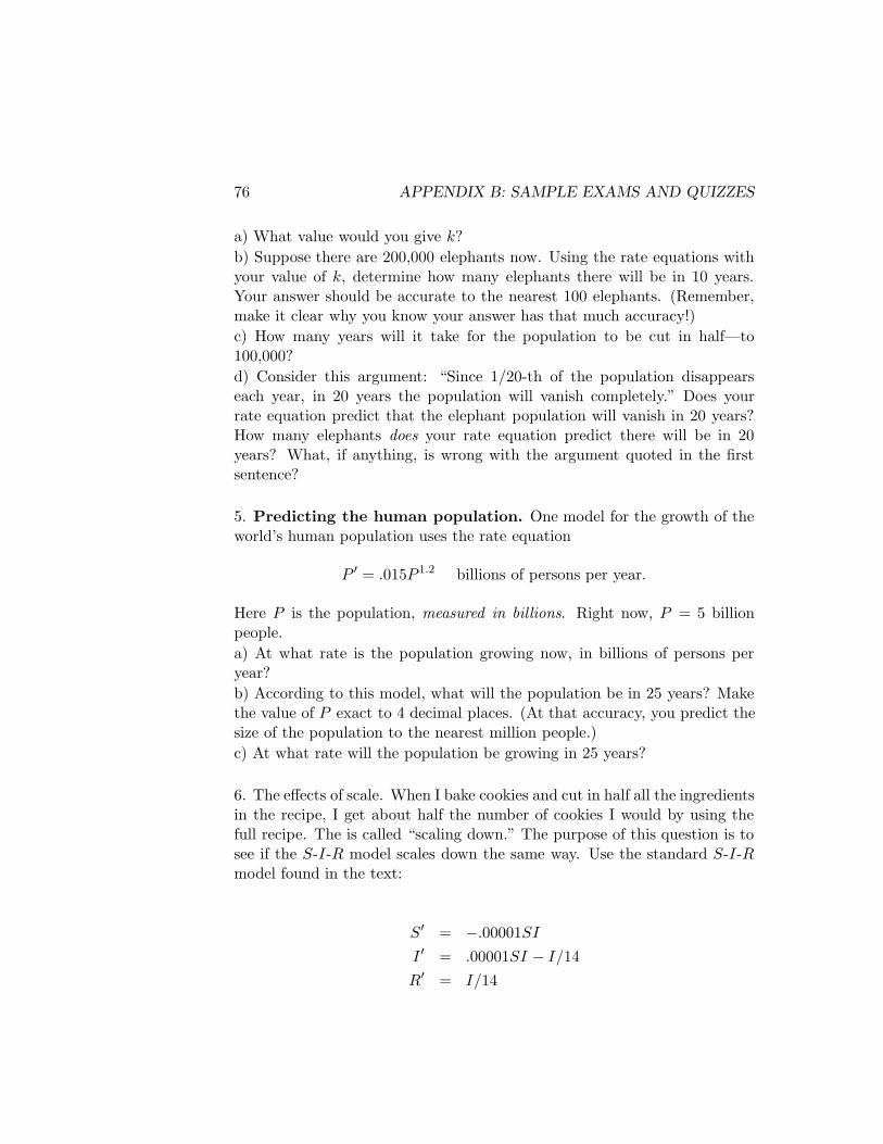
76 APPENDIX B: SAMPLE EXAMS AND QUIZZES

a) What value would you give k?

b) Suppose there are 200,000 elephants now. Using the rate equations withyour value of k, determine how many elephants there will be in 10 years.Your answer should be accurate to the nearest 100 elephants. (Remember,make it clear why you know your answer has that much accuracy!)

c) How many years will it take for the population to be cut in half—to100,000?

d) Consider this argument: “Since 1/20-th of the population disappearseach year, in 20 years the population will vanish completely.” Does yourrate equation predict that the elephant population will vanish in 20 years?How many elephants does your rate equation predict there will be in 20years? What, if anything, is wrong with the argument quoted in the firstsentence?

5. Predicting the human population. One model for the growth of theworld’s human population uses the rate equation

P ′ = .015P 1.2 billions of persons per year.

Here P is the population, measured in billions. Right now, P = 5 billionpeople.

a) At what rate is the population growing now, in billions of persons peryear?

b) According to this model, what will the population be in 25 years? Makethe value of P exact to 4 decimal places. (At that accuracy, you predict thesize of the population to the nearest million people.)

c) At what rate will the population be growing in 25 years?

6. The effects of scale. When I bake cookies and cut in half all the ingredientsin the recipe, I get about half the number of cookies I would by using thefull recipe. The is called “scaling down.” The purpose of this question is tosee if the S-I-R model scales down the same way. Use the standard S-I-Rmodel found in the text:

S′ = −.00001SI

I ′ = .00001SI − I/14

R′ = I/14

77

Take the initial values used in the text and cut them down by a factor of 10.Thus, the new initial values are

S = 4540, I = 210, R = 250

a) What is the value of S after 15 days? Compare this with the value of Safter 15 days when we use the original initial values (which were 10 timeslarger). In particular, is the new value of S equal to 1/10-th the originalvalue of S after 15 days? (In other words, does the value of S “scale down”the way a cookie recipe would?)b) Using the new initial values, sketch the graphs of S(t), I(t), and R(t)for 0 ≤ t ≤ 30 days. Compare these to the graphs of S, I and R fromthe original problem (in which the initial values were 10 times larger). Inparticular, do the new graphs have the same shape as the original graphs(“scaled down” by a factor of 10)?c) If the same epidemic (i.e., we’ll use the same model to describe it) strikesa large city and a small town, will the same effects be observed? Write abrief essay summarizing your conclusions about the effects of scaling on theS-I-R model. In particular, you know that the S-I-R model has a threshold.What is the conneciton between the scaling and the threshold?

78 APPENDIX B: SAMPLE EXAMS AND QUIZZES

CALCULUS ISAMPLE MIDTERM 1, in-class portion (75 minutes)

(week 5, on chapters 1 and 2)

This is a “closed-book” test; no books or notes are allowed. You may use acalculator if you wish.

1. Find a formula for the linear function y = f(x) that satisfies the conditionsf(3) = 0 and f ′(0) = −2.

2. The growth of the population P of a small town is modelled by the rateequation P ′ = .02P persons per year. Assume that P = 1000 when t = 0.In each of (a) and (b), organize your work in a table.a) Use a single calculation with ∆t=4 to estimate P (4).b) Use two rounds of calculations with ∆t=2 to estimate P (4).c) Illustrate your calculation in (b) with a graph of a piecewise linear functionthat approximates the graph of P on the interval 0 ≤ t ≤ 4. Label pointsand slopes.

3. [Provide a figure for this problem showing graphs of two positive functionsy = F (t) and y = M(t) in the first quadrant, each with a single maximum,and with the peaks at different values of t.]Consider the functions F (t) and M(t) of time t whose graphs are sketchedabove. Let tM be the time when M is at its maximum, and let tF be thetime when F is at its maximum.a) Which is larger: F (tM ) or M(tF )?b) At time tM , is F increasing or decreasing?c) At time tF is M increasing or decreasing?

4. Here are a succession of Euler approximations for the population P of acity after 3 years. [Provide a table of estimates of P (3) for values of ∆t =1.0, 0.1, 0.01, 0.001, 0.0001, 0.00001.] What is the most precise value youcan give for the exact value of P (3)? How many digits do you know exactly?Why are you sure they are exact?

5. In 1970 the Science Library had 81,000 volumes, and by 1975 the numberhad grown to 88,500.a) During 1970-75, the Science Library grew at a constant annual rate. Whatwas that rate, in volumes per year?

79

b) If the 1970-75 rate continued without change, how many volumes wouldthe Science Library have in 1990?c) The old building housing the science Library had a capacity of 105,000volumes. At the 1970-75 rate, when would it reach capacity?

6. A beaker contains three kinds of molecules called dimers, monomers andtrimers. The variables D, M and T keep track of the number of moleculesof each type. The following model describes how the numbers of each kindof molecule change over time.

D′ = .1M2 − .2MD

M ′ = −.1M2 − .2MD

T ′ = .2MD

Below are graphs of D(t), M(t) and T (t) (in some order). Label the graphswith D, M and T in a way that is consistent with this model.[Provide graphs like those on page 17 of the text.]

7. Around 1920 L.F. Richardson constructed a simple model to describean “arms race” between two countries. If x and y are the annual militarybudgets of the two countries (in billions of dollars), then the model expressesthe rates at which x and y change (in billions of dollars per year) in termsof the values of x and y. Consider two countries for which the model says

x′ = −4x + 2y

y′ = 5x − 4y + 12

and suppose this year x = 5 and y = 6.a) According to the model, will x increase or decrease next year? Will yincrease or decrease next year?b) Assuming the rates given in the model stay fixed for an entire year,estimate the values of x and y one year from now.c) According to the model, there are budgets x and y which will not change

from one year to the next. What are those values of x and y?

80 APPENDIX B: SAMPLE EXAMS AND QUIZZES

CALCULUS ISAMPLE MIDTERM 2, take-home portion

(week 9, on chapter 3 and 4.1, 4.2)

This is an “open-book” test; you may consult freely your notes, home-works, text, and any other books you wish; you may use a calculator or acomputer, and any programs available on a computer. However, you mustnot receive help, in any form, from anyone else. Make your responses briefbut complete; explain your reasoning, and write clearly.

1. a) Let H(x) = xx. Find H ′(2) to three decimal places accuracy.b) You know H(2) = 22 = 4. Use your answer to (a) to estimate the valueof 2.0152.015.c) Now use a calculator to determine 2.0152.015, and compare this with yourestimate. According to the calulator, how many digits of your estimate areaccuarate.

2. [Sketch a graph of y = f ′(x).] Sketched above is the graph of the derivative

of an unknown function f(x). Make an accurate copy of this graph on youranswer paper.There are many different functions f(x) whose derivative could be the graphshown above. On a separate coordinate plane just above your copy of f ′(x)sketch the graphs of two such functions f(x). Call them f1(x) and f2(x).Choose f2 so that it satisfies the additional condition f2(0) = 0.

3. The distance to the stars. When we look at an object, our two eyeshave slightly different views of it. This difference is called parallax. If theobject is close, the angle between the views is large (and we look “cross-eyed”). As the object moves farther away, the angle gets smaller. Our brainsenses the parallax angle and uses it to judge the distance to the object.

Astronomers use parallax to judge the distance to the nearby stars. Theytake two views of the star six months apart, and measure the angle 2θbetween the views. They call θ itself the parallax angle. Even thoughthe viewpoints are on opposite sides of the earth’s orbit (they are about 186million miles apart), θ is still very small. It is always less than 1” (one second,or 1/3600-th of one degree). If the parallax angle of a star is θ seconds, thenthe distance S to that star is

S =3.26

θlight-years.

81

(Note: A light-year is the distance light travels in one year; it is about6 trillion miles! Also, there is no need to measure θ in radians because nocircular functions are involved.)a) The parallax angle θ of the nearest star is 0.762”. How many light yearsaway is that star?b) Since θ is obtained by measurement, its value is never known precisely.Any error ∆θ in measuring θ will propagate to an error ∆S in the calculatedvalue of S. Write the error propagation equation for ∆S in terms of ∆θ.c) Suppose you measure the parallax of a star and then calculate that it is8.35 light-years away. If you want your calculation to be accurate to within.05 light-years, how precisely do you have to measure the parallax angle θ?d) Write the propagation equation for relative errors.e) If you want to calculate the distance to a star to within 1 %, what per-centage error can you tolerate in the measurement of the parallax angle θ?[Provide a figure showing the star as a point at the apex of an isoscelestriangle whose base is a diameter of the earth’s orbit around the sun. Theangle at the apex is 2θ, and the altitude is S.]

4. Fermentation. Do problems 8-11 on pages 172-174 of the text.

5. Falling bodies—with gravity and air resistance. Do problems 21-23on pages 197-198 of the text.

82 APPENDIX B: SAMPLE EXAMS AND QUIZZES

Calculus ISAMPLE MIDTERM 2, in-class portion (75 minutes)

(week 9, on chapter 3 and 4.1, 4.2)

This is a “closed-book” test; no books or notes are allowed. You may use acalculator if you wish.

1. The graph below shows a runner’s distance D in meters from the startingline after t seconds.[Provide a graph of distance versus time on a grid so coordinates can beread.]a) When is the runner speeding up? How can you tell?b) What is your best estimate of the runner’s velocity at t = 3? Be sure toinclude units.

2. [Provide a sketch of the graph of a function, as in exercise 1 of 3.5 on page134.] Copy the graph of the function f(x) above onto your answer paper.In a coordinate plane just below your graph of f , sketch the graph of thederivative of f .

3. Find formulas for the the derivatives of each of the following functions.[Choose a reasonable selection of four or five based on 3.5 and 3.6.]

4. a) Find the microscope equation for the function y =√

x at x = 100.b) Use (a) to estimate the value of

√99.3.

5. A block of ice is melting, and its volume shrinks at the steady rate of 15cubic inches per minute. Assume that the block of ice is a perfect cube. Atwhat rate is the length of the edge of the block decreasing when the edge is10 inches long? Be sure to include units.

6. Verify that

y(t) =1√

6 − 2t

is a solution to the initial value problem y′ = y3, y(1) = 1/2.

83

CALCULUS IFINAL EXAMINATION, take-home portion

(on chapters 1 - 6)

This is an “open-book” test; you may consult freely your notes, home-works, text, and any other books you wish; you may use a calculaator or acomputer, and any programs available on a computer. However, you mustnot receive help, in any form, from anyone else. Make your responses briefbut complete; explain your reasoning, and write clearly.

1. a) Determine the value of each of the following integrals to four digitsaccuracy.

∫ 1

0

1

1 + x2dx

∫ 2

−2e−x2

dx

b) Demonstrate how you know that the first four digits of your answers topart (a) are correct.

2. a) Until now, our only solutions to the logistic equation

dP

dt= kP

(

1 − P

C

)

have been provided by Euler’s method. In fact, though, the formula

P (t) =Cekt

1 + ekt

also provides a solution. Use algebra and the rules for differentiation toverify that this formula does indeed give a solution to the logistic equation.b) Suppose we extend the formula in part (a) to

P (t) =CAekt

1 + Aekt

where A is any number whatsoever. Verify that this extended formula isalso a solution to the logistic equation, for any value of A.c) In the formula for P (t), let k = 1, C = 12, and A = 2. Sketch the graphof y = P (t) on the interval 0 ≤ t ≤ 20. What is the value of P (0)?d) Find the formula P (t) for the solution to the initial value problem

dP

dt= .2P

(

1 − P

1000

)

P (0) = 200.

84 APPENDIX B: SAMPLE EXAMS AND QUIZZES

Sketch the graph of this solution over 0 ≤ t ≤ 20.

3. Growth in a seasonally fluctuating environment. You have alreadyconsidered the growth of a rabbit population R(t) that is governed by alogistic model:

dR

dt= .1R

(

1 − R

C

)

rabbits per month.

In this model, the carrying capacity of the environment was assumed tohave the constant value C = 25000 rabbits. However, it is reasonable tothink that the environment can support fewer rabbits in the winter thanin the summer. We can therefore make a more realistic model by havingC fluctuate periodically with the seasons. This question investigates whathappens to the population R(t) when the carrying capacity depends on timeaccording to this formula:

C(t) = 25000 − 5000 cos(πt/6) rabbits per month.

Here t measures the time in months since January 1990.a) Sketch the graph of C(t) for an interval of 60 months. Indicate on yourgraph the lowest value that C achieves, and the months when that occurs.Also indicate the peak value and the months when that occurs. How manymonths are there between one peak and the next? (This is called the period

of C, and C is said to be periodic.)b) Sketch the solution of the new logistic equation

dR

dt= .1R

(

1 − R

25000 − 5000 cos(πt/6)

)

for which R(0 = 2000 rabbits. Show at least the first 120 months. [Note:part (c) below asks you to make a second sketch of R(t) after completingparts (c) and (d).]c) After about 60 months, R(t) settles in to a fluctuating pattern that issimilar to the pattern of C(t)—that is, R(t) becomes periodic. Determinethe period of R(t), and compare it to the period of C(t). (This means:decide whether the two periods are the same, or whether one is larger thanthe other.)d) What are the peak and lowest values of R(t), and in what months do theyoccur? Compare the peaks of R and C. Are they the same size, or is onelarger? Which one? Do the peaks happen in the same month? If not, whichpeaks first, R or C? Compare the lowest values of R and C the same way.

85

e) Summarize your findings in parts (c) and (d) by sketching on the samecoordinate plane the graphs of R(t) and C(t) over the interval 60 ≤ t ≤ 120.Your graphs should show how the peaks of R and C relate to each other.

4. Prices, demand and profit. Do problems 1 and 2 on pages 294-295.

5. [Draw a graph of f on a grid and choose values of A < B < C < Dappropriately for your graph and the questions below.]This question concerns the function f(x) whose graph appears above.a) Give a simple argument that shows

A ≤∫ 5

0f(x) dx ≤ D.

b) Give a more detailed argument that shows

B ≤∫ 5

0f(x) dx ≤ C.

86 APPENDIX B: SAMPLE EXAMS AND QUIZZES

Calculus IFinal Exam, in-class portion (time limit 2.5 hours)

(on chapters 1-6)

This is a “closed-book” test; no books or notes are allowed. You may use acalculator if you wish.

1. Find the indicated derivatives. [Choose a sample of four or five from 5.1,and one accumulation function from 6.4.]

2. Times are tough in the decaying mill town of Detroit, Oregon. Its popula-tion P is modelled by the differential equation P ′ = −.01P . The populationof Detroit was 2000 in 1990.a) Write a formula for P as a function of t, the time in years after 1990.b) Using this model, when will the population of Detroit fall to 1000?

3. Use Euler’s method with a step size of ∆t = .5 to estimate y(1.5) giventhat y(0) = 1 and y′ = y + 1.

4. Find the critical points and global extreme values (that is, the globalmaximum and minimum) of y = 1

3x3 − 2x2 + 2 on the interval −1 ≤ x ≤ 3.(Be sure to find both x and y coordinates.)

5. Write out and compute the Riemann sum for∫ 60 2x dx obtained by taking

3 subintervals of equal length and sampling at the midpoints of the subin-tervals.

6. Here is some information about the second derivative of a function f :

f ′′(x) > 0 for x < 2 and x > 1

f ′′(x) < 0 for − 2 < x < 1.

For each of the following functions f , indicate whether or not the graph isconsistent with the given information. Briefly explain each of your answers.[Provide three or four suitable graphs.]

7. Which of the following are solutions to the indicated initial value problem?Be sure to explain your answer in each instance.a) Is y = 1

3t3 − 2 a solution to y′ = t2, y(3) = 7?

87

b) Is y = 2e3t a solution to y′ = 2y, y(0) = 2?c) Is y =

∫ t2 ln(x) dx a solution to y′ = ln(t), y(2) = 0?

8. Use the Fundamental Theorem to find the exact value of the followingdefinite integrals. [Choose 2 from 6.4.]

9. The following is the graph of the velocity (in units of 10000 km/sec) ofan electron in a particle accelerator against time. Approximately how fardoes the particle travel from t = 0 to t = 6? Explain clearly how you arecalculating your estimate. [Provide a suitable graph of velocity versus time,with a grid so that coordinates can be read.]

10. Suppose that you know f(1000) = 375 and f ′(1000) = −25. Use thisinformation to estimate f(998).

11. After sketching graphs of a function f(x) and its derivative f ′(x), a tiredstudent spilled her coffee on the graph of f(x), and part of the graph wasobliterated, as shown.[Provide a partial graph of f on one coordinate plane, and a complete graphof f ′ on a plane just below it.]Please redraw the graph of f(x) for the student, using her graph of f ′(x) asa guide.

88 APPENDIX B: SAMPLE EXAMS AND QUIZZES

Calculus ISample Quizzes (15-20 minutes each)

QUIZ 1 (on 1.1)Consider an epidemic modelled by the rate equations

S′ = −.00002SI

I ′ = .00002SI − I/5

R′ = I/5

with initial values (i.e., values for “today” t = 0)

S = 20, 000 I = 100 R = 100

1. Organize your work and your answers for this problem in a single tablefor t, S, I,R, S′, I ′, R′.a) Use the model to find values of S, I, and R tomorrow.b) Use your results in (1) to find values of S, I, and R the day after tomorrow.

2. Redo your calculation of the values of S, I, and R the day after tomorrowusing a single time step of two days. Again, organize your work and youranswers in a table.

3. For this model with these initial values, the graph of I versus t appearsbelow. On a certain day—call it day T—the model says the number ofsusceptibles is S(T ) = 6, 000. Is day T before or after the infection peaks?How can you tell?[Provide a graph like the graph of I on page 3 of the text.]

QUIZ 2 (on 1.2)1. Find the equation of the straight line passing through the points (−1, 5)and (1, 9).

2. The volume V of a quantity of gas at atmospheric pressure is a linearfunction of its temperature T in degrees (centigrade). The gas occupies 500cubic centimeters when the temperature is 10 degrees, and it fills 1300 cubiccentimeters when the temperature is 12 degrees.a) Find the slope = rate of change = multiplier of this linear function (includeunits).

89

b) If the temperature goes up by 10 degrees, by how much will the volumeincrease?

c) What temperature chanage would shrink the volume by 100 cubic cen-timeters?

QUIZ 3 (on 1.3)

1. The amount R of radium (measured in grams) in a sample changes overtime (measured in years). The rate R′ at which the radium changes intolead is proportional to the amount of radium present. Measurements showthat R′ = −(1/2337)R. Assume that you begin with a sample containing 10grams of radium. Modify the attached copy of the program SIR to estimatethe amount of radium in the sample after 5 years, using a time step of .5year. Cross out lines of the program you don’t need. Next to each line ofthe program that you need to change, write the appropriate variation.

[Provide a copy of SIR as on page 44 of the text.]

2. The variables S, I,R, S′, I ′, R′ have their usual meanings in a model ofthe spread of an epidemic. Use the data sheet provided showing the esti-mated values of these variables over a 20 day period to answer the followingquestions. For each question, specify which variable you looked at to answerthe question.

[Provide a printout of the values of the variables; label the columns with thevariable names.]

a) On which day did the epidemic peak?

b) On which day did the largest number of persons fall ill?

c) On which day did the largest number of persons recover?

QUIZ 4 (on 3.1 and 3.2)

1. A question estimating a rate from a table of values, like problem 5 onpage 94.

2. A question estimating a rate from a graph, like problem 9 on page 105.

QUIZ 5 (on 3.3 and 3.5)

1. A microscope equation problem, like one of those on page 120.

2. Given the graph of a function, sketch a graph of its derivative (likeproblem 5 on page 134).

QUIZ 6 (on 3.5)

90 APPENDIX B: SAMPLE EXAMS AND QUIZZES

1. Find formulas for the derivatives of the following functions [choose twolike those in problem 6, page 134].

2. Write the microscope equation for y = f(x) at x = a and use it toestimate the value of the function at x = a + h [choose one like problem 12or 15 on page 136].

3. A motorized toy car is moving along a straight track. Its distance (ininches) from the starting point is given by D = 3t2 + 18

√t + 5t, where t is

the number of seconds the car has been moving. What is the velocity of thecar after 9 seconds have passed? (include units)

QUIZ 7 (on 4.3)1. Differentiate the following functions [choose two like those in problem 3on page 210].

2. Check that y = 300e.1t is a solution to the initial value problem y′ = .1yand y(0) = 300.

3. The per capita growth rate of Afghanistan was .0216 in 1985, and thepoulation then was 15 million people. The initial value problem P ′ = .0216Pand P (0) = 15 summarizes this information (assuming t = 0 in 1985). Writea formula for P that is a solution to this initial value problem. (You don’tneed to check your solution.)

QUIZ 8 (on 4.4)1. Determine the numerical value of each of the following [two like problem1 on page 227].

2. Solve for x in the following equation: 4e3x = 15.

3. Find dy/dx for y = ln(2x3 + 7x).

QUIZ 9 (on 5.3)1. On the following graph of f(x) on the interval [a, b], mark with an ×(directly on the graph) all critical points of f . [Provide a suitable graph.]

2. Find the critical points of f(x) [one or two like problem 7 on page 274,but without sketching the graph or analyzing the critical points].

91

CALCULUS IISAMPLE MIDTERM 1, take-home portion

(week 4 or 5, on chapters 7 and 11.1-11.3, 12.3)

This is an “open-book” test; you may consult freely your notes, home-works, text, and any other books you wish; you may use a calculator or acomputer, and any programs available on a computer. However, you mustnot receive help, in any form, from anyone else. Make your responses briefbut complete; explain your reasoning, and write clearly.

1. Do problem 12 on page 402 (soft spring).

2. Do problem 16 on page 403 (first integral for soft spring).

3. Do problem 27 on page 405 (predator prey—May model).

4. Do problem 23 on page 625 (finding the value of an accumulation functionwith a differential equation solver).

5. a) Obtain a formula for the Fourier sine transform of f(x) = x on theinterval 0 ≤ x ≤ 1. That is, determine

Fs(ω) =

∫ 1

0x sin(2πωx) dx .

b) Sketch the graph of y = Fs(ω) on the interval 0 ≤ ω ≤ 5. At what pointω on this interval does Fs(ω) attain its maximum? What is the maximum?

92 APPENDIX B: SAMPLE EXAMS AND QUIZZES

Calculus IISAMPLE MIDTERM 1, in-class portion (time limit 75 minutes)

(week 4 or 5, on chapters 7 and 11.1-11.3, 12.3)

This is a “closed-book” test; no books or notes are allowed. You may use acalculator if you wish.

1. Questions on period and/or amplitude (like problems 1 or 4 on page 379).

2. a) Show that E = 12v2 + 1

2b2x2 is a first integral for the linear spring

x′ = v x(0) = a

v′ = −b2x v(0) = p

b) If v = 0, what is the value of x? (Your answer will be in terms of theparameters a, b and p.)c) Use the first integral to show the solution to this system of differentialequations is periodic.

3. Find a formula for each of the following integrals.[Include a selection of 5 or 6 indefinite and definite integrals drawn from11.1-11.3.]

93

CALCULUS IISAMPLE MIDTERM 2, take-home portion(week 9, on chapters 8 and 11.1, 11.4, 12.1)

This is an “open-book” test; you may consult freely your notes, home-works, text, and any other books you wish; you may use a calculator or acomputer, and any programs available on a computer. However, you mustnot receive help, in any form, from anyone else. Make your responses briefbut complete; explain your reasoning, and write clearly.

1. The value of the integral

J =

∫ ∞

1xp dx

depends on the value of p. For example, if p = −2 then J = 1, while if p = 1then J = ∞.a) Determine all values of p for which J = ∞.b) Determine all values of p for which J is finite, and determine the value ofJ .

2. Predator-prey interactions with harvesting. The basic models ofpredator-prey interactions take no outside environmental factors into ac-count. This question adds one such factor—the effects of certain humanintervention, called harvesting with equal effort.

Consider a population of insects, such as moths, that damage an agri-cultural crop. Suppose the moths are kept under control naturally by apredator—in this case, spiders. But suppose the crop is sprayed repeatedlywith an insecticide like DDT, to reduce the moth population even more.Does the strategy work? The problem is that both spiders and moths diefrom the poison, so the DDT may do more harm than good.

Here is another example, connected with Volterra’s original studies offish catches in the Adriatic sea. One species preys upon the other, and bothare caught in nets. Continual fishing reduces the breeding population of eachspecies. How does this affect the sizes of the two populations?

Proceed in the following way. Assume that the orignal predator-prey in-teraction is modelled by the standard equations in which the prey populationgrows logistically in the absence of predators:

x′ = ax

(

1 − x

K

)

− bxy

y′ = cxy − ey

94 APPENDIX B: SAMPLE EXAMS AND QUIZZES

Here x and y are the sizes of the prey and the predator populations, re-spectively. Spraying or fishing (or, more generally, “harvesting”) removes afraction of the breeding populations of both species. In the absence of anymore precise information, we assume it is the same fraction—h. (This iswhat we mean by harvesting with “equal effort.”) Thus we must decrease x′

by hx and y′ by hy. Making these modifications to the basic equations, weget

x′ = ax

(

1 − x

K

)

− bxy − hx

y′ = cxy − ey − hy.

Now carry out an analysis of the following concrete problem:

x′ = .1x

(

1 − x

2500

)

− .005xy − hx

y′ = .00004xy − .04y − hy.

a) Assume first that h = 0. That is, examine the model before any harvestingoccurs. Make a sketch in the (x, y)-plane that shows where x′ = 0 and wherey′ = 0. Find the equilibrium points of this system, and mark them clearlyon your sketch.b) Suppose we begin with x = 2000 and y = 10. What happens to x and yover time?c) Now harvest the populations by setting h = .02. Make a new sketch inthe (x, y)-plane that shows the new places where x′ = 0 and y′ = 0, and findthe new equilibrium values of x and y.d) Suppose we again start with x = 2000 and y = 10 but have a harvestingeffort of h = .02. What happens to x and y now?e) The basic model (with h = 0) has an equilibrium with both predators andprey present (that is, x > 0 and y > 0). What happens to this equilibriumwhen harvesting occurs? At the new equilibrium, are there more or fewerpredators, and are there more or fewer prey?f) Does the model sugggest that fishing increases the proportion of predatorspecies in relation to the prey, or is it the other way around?g) Does the model support the use of DDT to reduce the population ofmoths? Explain your position clearly.

3. The Richardson arms race model. Between the two World Wars, theBritish physicist Lewis Fry Richardson devised a simple model to describe

95

the “arms races” carried on by various nations at various times. It concernstwo aggressively hostile countries or alliances of countries; call them X andY . Let x(t) represent the level of hostile activity of X at any time t, andlet y(t) represent the same for Y . For example, take x to be the annualarmaments budget of X in billions of dollars, and measure t in years. Thereare diverse political pressures in X, some tending to make x increase, sometending to make it decrease. The same is true in Y . Richardson concentrateson three sources of pressure:

1. The larger y is, the greater the pressure to increase x. [An example: inthe 1980’s, the U.S. navy grew in size, partly because the Soviet navygrew.]

2. The larger x is, the greater the pressure to reduce x. [An example:it is costly for the U.S. to maintain large garrisons around the world;some in Congress argue the money would be better spent supportingsocial programs at home.]

3. Citizens of X may have a grievance against Y , independent of the sizeof either’s armaments expenditures. [An example: Until quite recently,communism was widely considered to be repugnant in the U.S., andthe Soviet Union was labelled “an evil empire.”]

Richardson assumes that x changes in response to each of these pressures,and he expresses the rate at which x achanges by the following differentialequation (representing, in order, each of the three sources of pressure listedabove):

x′ = ay − mx + g

A similar equation describes how y changes:

y′ = bx − ny + h

The values of the coefficients a, b, m, n, g and h are to be determined bythe circumstances of a particular case.

Now, consider two possibilities: in the first, the type 2 pressures arelarger than the type 1 pressures for both X and Y . In other words, eachprefers to spend its money on domestic needs rather than armaments. Hereis a specific example:

x′ = .1y − .3x + 4

y′ = .2x − .5y + 3

96 APPENDIX B: SAMPLE EXAMS AND QUIZZES

For the second possibility, suppose that the pressures for X are reversed,while those for Y are unchanged:

x′ = .3y − .1x + 4

y′ = .2x − .5y + 3

a) For each of the two specific possibilities, determine whether there arehostility levels x and y for which the various pressures exactly balance, sothat x and y do not change over time. If so, what are those levels?b) Suppose the current hostility levels are x = 10 and y = 20. For each ofthe two specific possibilities, what are the hostility levels after one year andafter two years? What happens in the long run?c) What is the essential difference between the two possiblities presentedabove. Explain how the outcomes are different, and explain why they aredifferent.

4. Problem 7(a)-(c) on pages 698-699 (one-dimensional random walk, usingStirling’s formula).

97

Calculus IISAMPLE MIDTERM 2, in-class portion (time limit 75 minutes)

(week 9, on chapters 8 and 11.1, 11.4, 12.1)

This is a “closed-book” test; no books or notes are allowed. You may use acalculator if you wish.

1. Consider the function f(x) = x5 − 4x2 + 7. Suppose that g(x) is theinverse function for f . a) What is f(1)? What is g(4)?b) What is g′(4)?

2. Use the method of separation of variable to find formulas for the solutionsof the following differential equations. [Choose two or three like problem 2,page 653.]

3. A warming liquid. [Use a variation of problem 3 on page 653.]

4. Logistic growth. [Use a variation of problem 13 on page 656.]

5. Assume we have three initial value problems, each defining solutionsx = x(t) and y = y(t). Below are graphs of their solutions x(t) and y(t)versus t, labelled (a), (b) and (c). There are three more graphs which showthe trajectories corresponding to each of these solutions in the state spacewhich is the x, y-plane. These are labelled (i), (ii) and (iii). Match eachof the graphs (a)-(c) to the corresponding graph (i)-(iii), and explain yourreasons for matching them as you do.[Provide the six graphs; include, for example, a periodic solution, a solutionthat stabilizes, and a solution with damped oscillation.]

98 APPENDIX B: SAMPLE EXAMS AND QUIZZES

CALCULUS IIFINAL EXAMINATION, take-home portion

(on chapters 7-12, emphasizing 9 and 10)

This is an “open-book” test; you may consult freely your notes, home-works, text, and any other books you wish; you may use a calculaator or acomputer, and any programs available on a computer. However, you mustnot receive help, in any form, from anyone else. Make your responses briefbut complete; explain your reasoning, and write clearly.

1. The function E defined by

E(x) =2√π

∫ x

0e−t2 dt

is called the error function (and is important in mathematical statistics).Find its Taylor series centered at a = 0.

2. Use Taylor’s theorem to estimate 3√

e to 4 decimal places. Carefully justifyyour choice of the degree of the approximating Taylor polynomial.

3. A ball is dropped from a height of 1 meter onto a smooth surface. On eachbounce, the ball rises to 60 percent of the height it reached on the previousbounce. Find the total distnace the ball travels. (Hint: be careful—draw apicture.)

4. Consider the function f(x, y) = x3 + y3 − 12(x + y).a) Find all critical points of f and determine the type of each.b) Sketch representative level curves of f in the (x, y)-plane on the domain−7 ≤ x ≤ 7, −7 ≤ y ≤ 7. Be sure to include the zero level. Mark each levelthat you draw with the value of f on that level.c) Mark the location of each critical point of f on your sketch. Indicate howthe pattern of level curves around a critical point confirms its type, as youdetermined in part (a).

5. Use the function f from problem 4 to construct the vector field grad f .Recall that the gradient field defines a dynamical system:

dx

dt=

∂f

∂x(x, y)

dy

dt=

∂f

∂y(x, y)

99

a) Sketch representative vectors and trajectories for this vector field of thedomain −7 ≤ x ≤ 7, −7 ≤ y ≤ 7.Comment: Vectors and trajectories of grad f should be perpendicular to thelevel curves of f that you found in question 4. Is this so?b) Find all the equilibrium points of grad fc) Some trajectories of grad f go to the local maximum of f . Mark on yoursketch all starting points for trajectories that go to this local maximum.

100 APPENDIX B: SAMPLE EXAMS AND QUIZZES

Calculus IIFinal Exam, in-class portion (time limit 2.5 hours)

(on chapters 7-12)

This is a “closed-book” test; no books or notes are allowed. You may use acalculator if you wish.

1. Evaluate each of the following integrals. [Choose an assortment of 5 or 6from 11.1-11.4 and 11.7.]

2. Find a formula for the solution to the initial value problem

y′ = 3t2y y(0) = 5

3. a) Let f(x) = e3x. Write a polynomial P (x) of degree 2 satisfyingP (0) = f(0), P ′(0) = f ′(0), and P ′′(0) = f ′′(0).b) Find a Taylor polyomial of degree 7 for

∫

ex2

dx

4. Determine the value of each of the following infinite sums.[Choose two like parts of problems 1 or 2 on pages 588-589.]

5. Find the radius of convergence of each of the following.[Choose two like parts of problems 10 or 11 on page 593.]

6. Write a sentence or two explaining why we studied the harmonic series.

7. Use Taylor polynomials to find an estimate for cos(.1) that is accurateto 3 decimal places. Explain how you know your answer has this accuracy(other than by comparing to what your calculator gives you for cos(.1)).

8. The variables x and y represent the sizes of two populations, one of whichpreys on the other. The way these two populations change over time ismodelled by the differential equations

x′ = ax + bxy

y′ = cy − dxy

101

where a, b, c and d are positive parameters. Which variable represents thepredator and which the prey? How can you tell?

9. [A microscope equation problem like one of problems 34-56 on pages496-499.]

10. The following questions refer to the contour plot of z = f(x, y) below.[Draw a contour plot with a local maximum and a saddle like the one onpage 512; mark a point P on the top edge.]a) Mark the critical points of f .b) Assuming that f has a local maximum, draw several gradient vectors off .c) Draw on the contour map the quickest path down from the local maximumto the point P . What principle guides this path?

102 APPENDIX B: SAMPLE EXAMS AND QUIZZES

Calculus IISample Quizzes (15-20 minutes each)

QUIZ 1 (on 7.2)1. What are the amplitude, period and frequency of f(x) = 6 sin(5x)?

2. Use the definition of the circular functions to explain the following.a) sin(3π/2) = −1b) cos(−t) = cos(t)

QUIZ 2 (on 11.1)1. Find a formula for each of the following indefinite integrals.[Choose two like parts of problem 10 on page 621.]

2. Find the area under the curve y = f(x) for x between a and b.[Choose one like problem 24 or 25 on page 625.]

QUIZ 3 (on 11.2)[Choose two like parts of problems 1 or 2 in on pages 632-633.]

QUIZ 4 (on 11.3)[Choose two like parts of problem 1 on pages 637-638.]

QUIZ 5 (on 8.1)[Choose a simple system of differential equations like problem 1a on page424.]a) Draw (in red) the set of points where R′ = 0, and mark the regions whereR′ > 0 and R′ < 0.b) Draw (in blue) the set of points where F ′ = 0, and mark the regionswhere F ′ > 0 and F ′ < 0.c) Mark any equilibrium points.d) Sketch representative vectors of the vector field.

QUIZ 6 (on 11.1)1. Sketch the graphs of y = 2x + 5 and its inverse on the same axes.

2. a) Sketch the graphs of y = f(x) = x2 for x ≥ 0 and its inverse y = g(x)on the same axes.b) What is the slope of f at x = 3?c) What is the slope of g at x = 9? Answer this question without differenti-ating g.

103

QUIZ 7 (on 11.4)1. Separation of variables—choose one like one part of problem 2 on page653.

2. Partial fractions—choose one like one part of problem 10 on page 656.

QUIZ 8 (on 10.2)1. Find a Taylor polynomial from the definition—choose one like problem 6on page 548.

2. Find a Taylor polynomial for an anti-derivative—choose one like part ofproblem 1 on page 548.

QUIZ 9 (on 10.4)Find a power series solution for a differential equation—choose one like partof problem 1 on page 571.

104 APPENDIX B: SAMPLE EXAMS AND QUIZZES

Appendix C: Drill Sheets

Here is a list of the supplementary drill sheets, with an indication in paren-theses of the section in the book they are appropriate for. You should feelfree to photocopy them for your own use.

page

(1.2) Equations of Lines . . . . . . . . . . . . . . . . . . . . . . . . . . . . . . . . . . . . . . . . 107*

(1.2) Solution sheet for the preceding . . . . . . . . . . . . . . . . . . . . . . . . . . . 108*

(1.2) A Drill Sheet on Lines (2 pages) . . . . . . . . . . . . . . . . . . . . . . . . . . 109

(1.2) One-a-Day Functions (2 pages) . . . . . . . . . . . . . . . . . . . . . . . . . . . 111

(3.2) The Microscope Equation . . . . . . . . . . . . . . . . . . . . . . . . . . . . . . . . . 113

(3.5) Differentiation Practice for 3.5 . . . . . . . . . . . . . . . . . . . . . . . . . . . . 114

(3.5 and 3.6) Differentiation Practice for 3.5 and 3.6 . . . . . . . . . . . . 115

(4.3) Thinking Exponentially . . . . . . . . . . . . . . . . . . . . . . . . . . . . . . . . . . . 116

(5.1) Differentiation Practice for 5.1 (2 pages) . . . . . . . . . . . . . . . . . . 117

(6.4) Integration Practice for 6.4 . . . . . . . . . . . . . . . . . . . . . . . . . . . . . . . 119

(11.1–11.3) Integration Practice for 11.1–11.3 . . . . . . . . . . . . . . . . . . . 120

* not in this document version

105

106 APPENDIX C: DRILL SHEETS

109

A Drill Sheet on Lines

1. Circle the points that lie on the line y = 5x + 2 :

(0, 2) (−25 , 0) (3, 17) (17, 3) (−1,−3) (−1

2 ,−12 )

2. The line which passes through the points (1, 2) and (7, 8) has slope; its equation is y = x+ ; and it also passes through

the points (16, ) , ( , .6), and (0, ).

3. a) Specify a couple of other points on the line which passes through(1, 1) and has slope 3: ( , ) , ( , ) .

b) What is the equation of this line?

4.T F Lines are parallel if they have the same slope.T F There is only one straight line passing through the points

(2, 17) and (−3, 5).

5. At what point do the lines y = 2x − 1 and y = x + 3 intersect?

6. What is the equation of the line passing through the points (5, 3) and(10, 23) ?

7. a) A line with slope 3 passes through the point (2, 5) ; it also passesthrough the points (3, ) , (2.1, ) , (1.8, ) , and (2 +a, ) . (You should do these without first finding the equation ofthe line.)

b) If, as it passes through the point (1, 17) a curve is approximately astraight line with slope 3, approximately what will the second coordinatey be if (1.001, y) is to lie on the curve?

8. Knowing that the freezing temperature of water is 0◦ Celsius and 32◦

Fahrenheit, and that water boils at 100◦ Celsius and 212◦ Fahrenheit, seeif you can figure out the formula which converts from one scale to another.(Hint: If you think of graphing Celsius temperatures along one axis and thecorresponding Fahrenheit temperatures along the other axis, what sort offigure would you get? Do you know any points on this figure? Why is thisexactly the same kind of problem as problem 6?)

110 APPENDIX C: DRILL SHEETS

9. Which of the following functions would you expect to have straight linegraphs?a. the cost of a taxi ride as a function of its length in milesb. the height of a tree as a function of its agec. the number of liters as a function of the number of pintsd. the circumference of a circle as a function of its radiuse. the area of a circle as a function of its radiusf. the population of the earth as a function of timeg. the logarithm of the population of the earth as a function of timeh. the value of a car as a function of its age

111

One-a-Day Functions

Here are some problems which have appeared in virtually every calculusbook written over the last thirty years. For each problem you should

• (Except for problems 4 and 6.) Draw a simple picture labelling thedifferent variables you are using and their relation to each other.

• Find the general functional relationship between the variables.

• Identify the domain of the function that makes physical sense.

• Sketch what you think the graph of the function looks like—looking atthe edges of the domain is often helpful in this. Then use the computerto graph the function, and compare this with your sketch. With thecomputer, locate interesting points, such as maxima and minima andexplain why these points might be of interest in the context of theproblem.

1. A farmer has 90’ of fencing out of which she plans to make a rectangularsheep pen up against the side of her barn, using the barn itself for one sideof the pen and the fencing for the other three sides. (The barn is 100’ long.)The total area A of the pen will thus vary with the shape of the rectangleformed. Let x be the length of the pen along the barn.

(Can you think of a simple way to find the value of x giving the maximumarea without using the computer (or calculus)?)2. Suppose we want to make a topless box with a square bottom and rect-angular sides, holding 80 cubic inches. The amount of material needed tomake the box is essentially the same as the surface area of the box. Howdoes the surface area of the box depend on the length of the bottom edge?3. A lighthouse is 8 miles off shore, the coast line being straight. Fifteenmiles up the beach is a town. Suppose the lighthouse keeper can row at therate of 2 mph and can walk at the rate of 4 mph. If he rows his boat tosome point on shore and then walks to town, how does the total time of thetrip depend on where he beaches his boat?4. A truck is to be driven 300 miles at a constant speed of x mph. Speedlaws require 30 ≤ x ≤ 65 (on a rural highway). Assume diesel fuel costs 90cents/gallon and is consumed at the rate of 2 + (x2/200) gallons/hour. Listsome of the features of this model for the rate at which fuel is consumedand explain why the model is or is not reasonable. If the driver’s wages are$16/hour, how does the total cost of the trip vary with the speed x?

112 APPENDIX C: DRILL SHEETS

5. Suppose we want to make a poster containing 50 square inches of printedmatter surrounded by a 3 inch border at the top and bottom, and a 2 inchborder along each side. How does the total area of the poster depend on thewidth of the printed matter?6. Suppose a manufacturer of plastic wombats figures out that the numberN of wombats she can sell at a price of p cents each is given by the rule

N(p) =

{

400(1 − (p/50)) if 0 < p < 500 if 50 ≤ p

and that the cost per wombat is given by C(N) = (100N + 200)/(5N + 2)cents. List some of the key features of these models for N(p) and C(N) andexplain why each model is or is not reasonable. Express her total costs andincome in terms of the unit price p. How does her profit depend on p?7. A piece of wire 30” long is cut into two pieces. One piece is bent intoa square, the other into a circle. Express the sum of the areas of the twofigures as a function of the length of the piece that is bent into a square.8. We want to make a nice Roman window in the shape of a rectanglesurmounted by a semicircle. If the perimeter of the window is to be fifty feet,how does the area of the window depend on the diameter of the semicircle?9. A 6 foot fence stands 8 feet away from a building wall. A ladder leaningon the top of the fence just reaches the building wall. Express the length ofthe ladder as a function of the distance from the foot of the ladder to thebottom of the fence.

113

The Microscope Equation

1. Suppose the volume of a right circular cylinder is:

V = hπr2

a) Find V when h = 6 cm and r = 2 cm.

b) If the height of the cylinder stays at 6 cm then V (r) = 6πr2. Use V (2)and V ′(2) to approximate V (2.1).

c) What is the microscope equation that you used in b)? (i.e., what is theapproximate change in V ?)

d) What is the exact value for V (2.1)? What is the exact value for ∆V ?

2. The edge of a cube is measured to be 10 cm with a possible error of.02 cm. Use the microscope equation to find an upper bound on the errorinvolved in calculating the volume of the cube to be 103 = 1000 cubic cm.

3. Use the microscope equation to approximate the following expressions,using a nearby point where the functions is known.

a) (9.06)1

2

b) (3.07)3

c) (48.8)1

2

d)1

1.98

e)1

311

5

f) (.000063)1

3

g) x2 + 2x − 3 at x = 1.07

h) (15).25

114 APPENDIX C: DRILL SHEETS

Differentiation Practice for 3.5

In problems 1–14, find formulas for the derivatives of the functions:

1. x5

2.√

x

3.1

x3

4. u7

5. 3√

w

6.1

z

7. 3x3 − 5x2 + 2

8. 5u3 − πu + 17

9. 1.7w −√w + 3

w2 − π

10. mx + b (m and b are constants)

11. −g2 t2 + v0t + d0 (g, v0, and d0 are constants)

12. 3 sin(x) + 2x3 − 5

13. −12 cos u + π2

14. tan z − 3 sin z + 2z5

15. The formula d = −16t2+10t+100 gives distance travelled as a functionof t. Find a formula for the velocity.

16. Use the derivative of y = x2 to explain why the graph of y has theshape it has: falling for x < 0, a minimum at x = 0, and increasing forx > 0.

17. (See the supplement to 1.2, problem 1) The formula for the area A ofthe sheep pen as a function of the length x along the barn is A = 45x− 1

2x2.

a) Find a formula for dA/dx

b) Use your formula from (a) to explain why x = .45 gives the maximumarea.

18. dy/dx = 6x2. What is a formula for y?

115

Differentiation Practice for 3.5 and 3.6

Differentiate the following functions:

1. cos 4w

2. sin 6t

3. x3 + 2 tan 5x

4. sin(ex)

5. 5 cos(1 − 2u)

6. tan(3z + 2)

7. sin(x2 + x + 1)

8. etan x

9. 2 sin6(3w)

10.√

sin(2x)

11. 7 cos3(4w)

12. 3√

3w − 5w5

13. cos2(√

1 + 2x)

14. 1/√

2x + 5

15. 8z2√z − 5 3√

z

16.5

(4x2 + 25)2/3

17.4

√

1

t

116 APPENDIX C: DRILL SHEETS

Thinking Exponentially

In the problems below, show all your work and your reasoning process.

1. Virtually all living things take up carbon as they grow. This carboncomes in two principal forms: normal, stable carbon—C12—and radioactivecarbon—C14. C14 decays into C12 at a rate proportional to the amountof C14 remaining. While the organism is alive, this lost C14 is continuallyreplenished. After the organism dies, though, the C14 is no longer replaced,so the percentage of C14 decreases exponentially over time. It is found thatafter 5730 years, half the original C14 remains. If an archaeologist finds abone with only 20% of the original C14 present, how old is it?

2. The human population of the world appears to be growing exponentially.If there were 2.5 billion people in 1960, and 3.5 billion in 1980, how manywill there be in 2010?

3. A cup of coffee at 80◦ C is placed in a room whose temperature is 20◦

C. After 10 minutes the temperature of the coffee is found to be 60◦. Ifwe assume that the rate at which the temperature difference changes isproportional to the difference, How long does it take for the temperature toreach 25◦? (Thus we are assuming that if the temperature of the coffee attime t is T (t), then the difference D(t) = T (t) − 20 satisfies the conditionD′(t) = −kD(t) for some constant k.)

4. If bacteria increase at a rate proportional to the current number, howlong will it take 1000 bacteria to increase to 10,000 if it takes them 17 minutesto increase to 2000?

5. Suppose sugar in water dissolves at a rate proportional to the amountleft undissolved. If 40 lb. of sugar reduces to 12 lb. in 4 hours, how longwill you have to wait until 99% of the sugar is dissolved?

6. Atmospheric pressure is a function of altitude. Assume that at any givenaltitude the rate of change of pressure with altitude is proportional to thepressure there. If the barometer reads 30 psi (pounds per square inch) atsea level and 24 psi at 6000 feet above sea level, how high are you when thebarometer reads 20 psi?

117

Differentiation Practice for 5.1

Differentiate the following functions

7. t2 · cos t

8.x3 − 2x

cos x

9.sinx

x3 − 5

10. ex(3x5 + 7x2)

11. 3e−z · sin(2πz)

12.(3t + 5)3

(4 − 7t)4

13. (x5 − 1)3(7x + 5)2

14.

√

4t + 7

2t − 3

15.tanw

w2 + 1

16. (3x5 + 7)(2x − 1)5

17. (15s + 3)(16s2 + s3)

18.x2

sin(x)

118 APPENDIX C: DRILL SHEETS

Differentiation Practice for 5.1—page 2

19. sin(x2)

20. sin(x) + x2

21.5x2 + ln(x)

7√

x + 5

22.6ecos(t)

5 3√

t

23. 3e7t + t − 17

24. Find partial derivatives of the following functions

a) x2 · sin(y)

b) sin(x2y)

c) ln(x + 2y)

d) exy

e)xy

x2y3 + 1

25. Write the microscope equation for

a) f(x) = 3x2 + 5x − sin(x) at x = 0

b) f(x, y) =y + cos(x)

3xy + 5at (0, 2)

26. Differentiate and SIMPLIFY:

a) (√

x − 1)e√

x

b) ln(x +√

1 + x2)

119

Integration Practice for 6.4

1. Do each of the following two ways: (i) by hand (using antidifferention)and (ii) using RIEMANN

a)

∫ 3

12x dx

b)

∫ 2

−1−3x2 dx

c)

∫ 2

0e3x dx

d)

∫ 3π/4

π/2cosx dx

e)

∫ π/4

π/8sin 2x dx

f)

∫ 3

2(x3 −

√x)dx

g)

∫ 2

−1(x2 + 3ex)dx

2. Let f(x) =

∫ x

1

1√1 + t2

dt

a) What is f(1)? What is the sign of f(x) for x > 1? What is the sign off(x) for x < 1?

b) Find a formula for f ′(x). Sketch a graph of y = f ′(x).

c) Find a formula for f ′′(x). Sketch a graph of y = f ′′(x).

d) Use the information in (a) - (c) to make a rough sketch of the graph ofy = f(x) on [−4, 4].

120 APPENDIX C: DRILL SHEETS

Integration Practice for 11.1-11.3

1.

∫ 4

2

√x +

3

xdx

2. F (x) =

∫ x

0t√

1 + t2 dt. Find a formula for F (x). Check that F ′(x) =

x√

1 + x2.

3.

∫

1

t2

√

1 − 1

tdx

4.∫

sin(2w) dw

5.∫

√

cos(x) sin(x) dx

6.∫

2e3x+2 dx

7.∫

(ex + e−x)2 dx

8.∫

es cos(es) ds

9.

∫

6

3x + 5dx

10.

∫

1

(2x + 3)2dx

11.

∫

3x2 − 2x

x3 − x2dx

12.∫

√

ln(x) dx

13.∫ 10 (e − ey)y dx

14. Find the area of the region under y = xe−x between 0 and 3.

15. Find the volume of the solid formed by rotating around the x-axis theregion under y = x3 between 0 and 2.

16. Find the distance travelled by a particle travelling with velocity v =2 cos(3t) for 0 ≤ t ≤ 1.

17. Solve the initial value problem y′ = 3e2t, y(0) = 5.

18. Write a Riemann sum approximating the area in #15, using 3 subin-tervals of equal length and sampling midpoints.

19. Do the same for #17, using 2 subintervals.

Appendix D: SupplementaryLaboratory Exercises

page

(2.1) Exact Values of S(1) and S(10) using SIRVALUE (2 pages) . . 123

(4.4) Logs and Exponentials (2 pages) . . . . . . . . . . . . . . . . . . . . . . . . . . . 125

(4.3) Graphing Exponential Functions . . . . . . . . . . . . . . . . . . . . . . . . . . . 127

(4.5) Euler’s Method for y′ = f(t) . . . . . . . . . . . . . . . . . . . . . . . . . . . . . . . 128

(6.4) Accumulation Functions (3 pages) . . . . . . . . . . . . . . . . . . . . . . . . . 129

This chapter is not in this document version

121

132 APPENDIX D: SUPPLEMENTARY LABORATORY EXERCISES

Appendix E: SupplementaryPrograms

Teachers vary considerably in the point at which they switch from computerprograms to commercial software. For those of you who like to continuethe use of programming in your course here are some additional programswhich are a bit more sophisticated than those in the text. They are writtenin TrueBasic, but can be readily adapted to other dialects. In additionto performing useful mathematical operations, these programs also containfeatures like drawing gridlines, using dialog boxes, and mouse input whichmake them more useful to students. These features can be left out if youwant a bare-bones utility.

Runge-Kutta Differential Equation Solvers If you choose notto move to fancier software for solving differential equations, one of themost useful programs you will need is a numerical method that convergesmore rapidly than Euler’s method. The most common improvement is the4th order Runge-Kutta method. The method essentially involves a moresophisticated weighting of the slopes in the neighborhood of the currentpoint to determine the direction and distance of the next step. Details canbe found in most numerical methods books. We give two versions. The first(RUNGE1.TRU) solves a simple first order differential equation and plots theresult in the t-x plane. The second (RUNGE2.TRU) solves a pair of linkeddifferential equations and plots the results in the x-y phase plane.

133

135

The example used in this program is the logistic equation

dx

dt= .1x (1 − x/10000) with x(0) = 500.

While x′ only depends on the value of x in this example, the method can beused unchanged for cases where x′ depends only on t, or on both x and t.For this reason, the defining function is written as func(x,t), even thoughonly x is involved in this case

RUNGE1.TRU

!!!!!!!!!!!!!! Specify initial values and functions

LET tinitial=0

LET tfinal=100

LET xmin = 0

LET xmax = 15000

LET numberofsteps = 1000

LET deltat = (tfinal-tinitial)/numberofsteps

DEF func(x,t) = .1 * x * (1 - x / 10000) !the rate of change function

!!!!!!!!!!!!!!! Subroutine to draw gridlines

SUB makegrid

SET COLOR "red"

LET numbhlines = 10 !number of horizontal grid lines

LET numbvlines = 20 !number of vertical grid lines

LET hspacing = (tfinal - tinitial)/numbvlines

LET vspacing = (xmax - xmin)/numbhlines

SET TEXT justify "left","half"

FOR k = 0 to numbhlines

LET x = xmin + k*vspacing

PLOT tinitial,x;tfinal,x

PLOT TEXT, AT tfinal-.8*hspacing, x:str$(truncate(x,3))

NEXT k

SET TEXT justify "center", "bottom"

FOR k = 0 to numbvlines

LET t = tinitial + k*hspacing

PLOT t,xmin;t,xmax

PLOT TEXT, AT t, xmin+.2*vspacing:str$(truncate(t,1))

NEXT k

END SUB

!!!!!!!!!!!!!!!! Set up the screen

SET WINDOW tinitial, tfinal, xmin, xmax

136 APPENDIX E: SUPPLEMENTARY PROGRAMS

SET BACKGROUND COLOR "yellow"

CALL makegrid

SET COLOR "red"

PLOT tinitial,0; tfinal,0 ! Draws the t-axis (in red)

SET COLOR "blue" !Specify color for graph

!!!!!!!!!!!!!!!! Run Runge-Kutta

LET t = tinitial

LET x = 500

PLOT t,x;

FOR K= 1 TO numberofsteps

LET k1 = func(x,t)*deltat

LET k2 = func(x + .5*k1,t + .5*deltat)*deltat

LET k3 = func(x + .5*k2,t + .5*deltat)*deltat

LET k4 = func(x + k3,t + deltat)*deltat

LET deltax = (k1 + 2*k2 + 2*k3 + k4)/6

LET t = t + deltat

LET x = x + deltax

PLOT t,x;

NEXT k

PRINT using "####.##### #####.#############":t,x

END

137

The example used solves the initial value problem

dx

dt= .15x(1 − .005x − .010y) and

dy

dt= .03y(1 − .004x − .005y),

with initial valuesx(0) = 30 and y(0) = 50.

Again, the defining rate equations could be specified to involve t also.

RUNGE2.TRU

!!!!!!!!!!!!!! Specify initial values, ranges, and functions

LET xmin = 0

LET xmax = 400

LET ymin = 0

LET ymax = 400

LET xinitial = 30

LET yinitial = 50

LET deltat = .1

LET numberofsteps =3000

!Enter the functions in the rate equations

DEF xprime(x,y) = .15*x*(1-.005*x-.010*y)

DEF yprime(x,y) = .03*y*(1-.004*x-.005*y)

!!!!!!!!!!!!!!! Subroutine to draw gridlines

SUB makegrid

(Here you would type in the grid-making subroutine similar to that in RUNGE1)

END SUB

!!!!!!!!!!!!!!!! Set up the screen and run program

LET hwidth = xmax - xmin

LET vwidth = ymax - ymin

SET WINDOW xmin-.05*hwidth, xmax+.05*hwidth,ymin-.05*vwidth,ymax+.05*vwidth

SET BACKGROUND COLOR "black"

CALL makegrid

!!! Put an ! in front of this line if you don’t want a grid

LET x = xinitial

LET y = yinitial

PLOT x,y;

FOR K= 1 TO numberofsteps

LET k1 = xprime(x,y)*deltat

138 APPENDIX E: SUPPLEMENTARY PROGRAMS

LET h1 = yprime(x,y)*deltat

LET k2 = xprime(x+.5*k1,y+.5*h1)*deltat

LET h2 = yprime(x+.5*k1,y+.5*h1)*deltat

LET k3 = xprime(x+.5*k2,y+.5*h2)*deltat

LET h3 = yprime(x+.5*k2,y+.5*h2)*deltat

LET k4 = xprime(x+k3,y+h3)*deltat

LET h4 = yprime(x+k3,y+h3)*deltat

LET deltax = (k1 + 2*k2 + 2*k3 + k4)/6

LET deltay = (h1 + 2*h2 + 2*h3 + h4)/6

LET y = y + deltay

LET x = x + deltax

PLOT x,y;

NEXT k

END

Remark: Note that RUNGE2 can be immediately used to solve a second orderdifferential equation in x by defining y = x′.

139

The previous program—Runge2—had the disadvantage that you had toreenter the program each time you wanted to plot a new trajectory to typein the coordinates of the starting point. Here is a program that allows thestudent to point and click with a mouse to specify the starting point for atrajectory in the phase plane. There is also a dialog box that prints thecoordinates of the starting point chosen and gives the student the option ofplotting a new trajectory after each run. Instead of using mouse input, adialog box could also be used to get the coordinates of the next trajectory.

PHASE.TRU

!!!!!!!!!!!!!! Specify initial values, ranges, and functions

LET xmin = 0

LET xmax = 400

LET ymin = 0

LET ymax = 400

LET deltat = .1

LET numberofsteps =2000

DEF xprime(x,y) = .15*x*(1-.005*x-.010*y)

DEF yprime(x,y) = .03*y*(1-.004*x-.005*y)

!!!!!!!!!!!!!!! Subroutine to draw gridlines

SUB makegrid

(Here again you would type in the grid-making subroutine similar to that in RUNGE1)

END SUB

!!!!!!!!!!!!!!!! Runge-Kutta approximation

SUB runge

PLOT x,y;

FOR K= 1 TO numberofsteps

LET k1 = xprime(x,y)*deltat !This would just be deltay in Euler’s

method

LET h1 = yprime(x,y)*deltat !This would just be deltayprime in

Euler’s method

LET k2 = xprime(x+.5*k1,y+.5*h1)*deltat

LET h2 = yprime(x+.5*k1,y+.5*h1)*deltat

LET k3 = xprime(x+.5*k2,y+.5*h2)*deltat

LET h3 = yprime(x+.5*k2,y+.5*h2)*deltat

LET k4 = xprime(x+k3,y+h3)*deltat

LET h4 = yprime(x+k3,y+h3)*deltat

LET deltax = (k1 + 2*k2 + 2*k3 + k4)/6

140 APPENDIX E: SUPPLEMENTARY PROGRAMS

LET deltay = (h1 + 2*h2 + 2*h3 + h4)/6

LET y = y + deltay

LET x = x + deltax

PLOT x,y;

NEXT k

END SUB

!!!!!!!!!!!!!!!! Set up the screen

LET hwidth = xmax - xmin

LET vwidth = ymax - ymin

OPEN #1:screen 0,1,.88,1

OPEN #2:screen 0,1,0,.87

SET WINDOW xmin-.05*hwidth, xmax+.05*hwidth,ymin-.05*vwidth,ymax+.05*vwidth

SET BACKGROUND COLOR "black"

CALL makegrid

WINDOW #1

RANDOMIZE

LET ans$="y"

DO while ans$="y"

WINDOW #2

SET COLOR 1+int(15*rnd)

GET POINT x,y

WINDOW #1

SET COLOR "white"

PRINT "Initial values: x= ";x; " y= ";y

WINDOW #2

CALL Runge

PLOT

WINDOW #1

PRINT "Final values: x= ";x;" y= ";y

INPUT prompt "Another? (y or n) ":ans$

CLEAR

LOOP

PRINT "done"

END

141

Here’s a program for quickly plotting a vector field (without arrow-heads!), with the additional possibility of zooming in by a factor of 10 on thecenter point. You could combine this program with features of the previousprogram–PHASE–to get a program which would plot trajectories in a vectorfield.

VECFIELD.TRU

!!!!!!!!!!!!!! Specify initial values, ranges, and functions

LET xcenter = 50 !coordinates of center of screen

LET ycenter = 50

LET screenhalfwidth = 50

LET deltat = 1 !you may need to fiddle with this to get it started right

DEF xprime(x,y) = .15*x*(1-.005*x-.010*y) !the functions in the differential

equation

DEF yprime(x,y) = .03*y*(1-.004*x-.005*y)

!!!!!!!!!!!!!!! Subroutine to draw gridlines

SUB makegrid

(Here again you would type in the grid-making subroutine similar to that in RUNGE1)

END SUB

!!!!! Subroutine to draw vector field

SUB arrows

FOR j = 0 to 20

FOR k = 0 to 20

LET x = xmin + j*hwidth/20

LET y = ymin + k*vwidth/20

PLOT x,y;x+xprime(x,y)*deltat,y + yprime(x,y) * deltat

NEXT k

NEXT j

END SUB

!!!!!!!!!!!!!!!! Set up the screen

OPEN #1:screen 0,1,.88,1

OPEN #2:screen 0,1,0,.87

LET ans$="y"

DO while ans$="y"

WINDOW #2

CLEAR

LET xmin = xcenter - screenhalfwidth

LET xmax = xcenter + screenhalfwidth

LET ymin = ycenter - screenhalfwidth

142 APPENDIX E: SUPPLEMENTARY PROGRAMS

LET ymax = ycenter + screenhalfwidth

LET hwidth = 2 * screenhalfwidth

LET vwidth = 2 * screenhalfwidth

SET WINDOW xmin-.05*hwidth, xmax+.15*hwidth,ymin-.05*vwidth,ymax+.05*vwidth

SET BACKGROUND COLOR "black"

IF screenhalfwidth > .001 then CALL makegrid

SET COLOR "yellow"

CALL arrows

WINDOW #1

SET COLOR "white"

INPUT prompt "Another? (y or n) ":ans$

CLEAR

LET deltat = deltat/10

LET screenhalfwidth = screenhalfwidth/10

LOOP

PRINT "done"

END

Appendix F: Solutions

This chapter is not in this document version

143