DDC of IPCC TGCIA Final Version - 10/30/03

Guidelines for Use of Climate Scenarios Developed from

Regional Climate Model Experiments

by

L. O. Mearns, F. Giorgi, P. Whetton, D. Pabon, M. Hulme, M. Lal

1. INTRODUCTION

For many regional and local applications, users of climate model results have long been

dissatisfied with the inadequate spatial scale of climate scenarios produced from coarse

resolution global climate model (GCM ) output (Gates, 1985; Robinson and Finkelstein, 1989;

Lamb, 1987; Smith and Tirpak, 1989; Cohen, 1990). This concern emanates from the perceived

mismatch of scale between coarse resolution GCMs (100s of km) and the scale of interest for

regional impacts (an order or two orders of magnitude finer scale) (IPCC, 1994; Hostetler, 1994).

For example, mechanistic models used to simulate the ecological effects of climate change

usually operate at spatial resolutions varying from a single plant to a few hectares. Their results

may be highly sensitive to fine-scale climate variations that may be embedded in coarse-scale

climate variations, especially in regions of complex topography, coastlines, and in regions with

highly heterogeneous land surface covers.

There are now techniques available for generating high resolution climate information,

but some tend to be complex and/or computationally expensive. It is also not always

straightforward which techniques one should use, or whether high resolution information is even

necessary for approaching certain types of impacts problems.

The purpose of this guidance material is to provide researchers in climate impacts with

the background material, and descriptions of procedures for evaluating, producing, and using

high resolution climate scenarios. We also provide recommendations for when and how to use

such scenarios. While we will present overview material on all downscaling or regionalization

methods, we will focus our more detailed discussions on regional modelling.

2

This guidance paper is not meant to be a manual or recipe book for actually producing

regional climate model (RCM) simulations. It is assumed that impacts researchers who are not

climate modelers, will be working with regional climate modelers who have the expertise for

generating such simulations. What we hope to do is inform the impacts researcher on choices

that can be made among techniques, on strengths and weaknesses of techniques, on what the

regional modelling community feels we know about the quality of simulations and on what

degree of confidence we have in the results of regional models compared to global coarse scale

models.

In this guidance document we present in part 2 background information on the different

methods of developing high resolution scenarios, in part 3 examples of how such scenarios have

been used up till now, and in part 4 a general discussion of the uncertainty of spatial scale in

relation to the many other uncertainties in climate impacts work. In part 5 we then go on to

explain the current thinking on the “added value” of high resolution information, provide

guidance on what should be considered in deciding whether to use a high resolution scenario,

and describe procedures for producing high quality regional modelling experiments. Finally in

part 6 we make general recommendations for use of RCM results for climate scenarios in

impacts work.

Much of the background information provided in this document is drawn from two

chapters of the IPCC Third Assessment Report, Working Group I volume, specifically chapter

10 on Regional Climate Information (Giorgi et al., 2001) and Chapter 13 on Climate Scenario

Development (Mearns et al., 2001). The reader is encouraged to review these chapters for more

in-depth discussion of some topics. Also the document Guidelines on the Use of Scenario Data

for Climate Impact and Adaptation Assessment available on the Data Distribution Centre Web

site (http://ipcc-ddc.cru.uea.ac.uk) contains general guidance on the use of scenarios, and should

also be read.

2. REVIEW OF METHODS

This section presents an overall discussion of the principles, objectives and assumptions

underlying the different techniques today available for deriving regional climate change

information. Table 1 provides a summary of climate scenario techniques that rely on the various

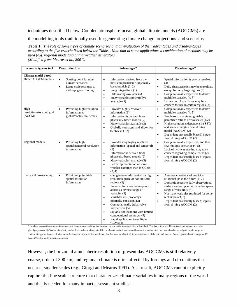
3

techniques described below. Coupled atmosphere-ocean global climate models (AOGCMs) are

the modelling tools traditionally used for generating climate change projections and scenarios. Table 1: The role of some types of climate scenarios and an evaluation of their advantages and disadvantages according to the five criteria listed below the Table. . Note that in some applications a combination of methods may be used (e.g. regional modelling and a weather generator). (Modified from Mearns et al., 2001).

Scenario type or tool

Description/Use Advantages* Disadvantages*

Climate model based: Direct AOGCM outputs • Starting point for most

climate scenarios • Large-scale response to

anthropogenic forcing

• Information derived from the most comprehensive, physically-based models (1, 2)

• Long integrations (1) • Data readily available (5) • Many variables (potentially)

available (3)

• Spatial information is poorly resolved (3)

• Daily characteristics may be unrealistic except for very large regions (3)

• Computationally expensive to derive multiple scenarios (4, 5)

• Large control run biases may be a concern for use in certain regions (2)

High resolution/stretched grid (AGCM)

• Providing high resolution information at global/continental scales

• Provides highly resolved information (3)

• Information is derived from physically-based models (2)

• Many variables available (3) • Globally consistent and allows for

feedbacks (1,2)

• Computationally expensive to derive multiple scenarios (4, 5)

• Problems in maintaining viable parameterizations across scales (1,2)

• High resolution is dependent on SSTs and sea ice margins from driving model (AOGCM) (2)

• Dependent on (usually biased) inputs from driving AOGCM (2)

Regional models • Providing high spatial/temporal resolution information

• Provides very highly resolved information (spatial and temporal) (3)

• Information is derived from physically-based models (2)

• Many variables available (3) • Better representation of some

weather extremes than in GCMs (2, 4)

• Computationally expensive, and thus few multiple scenarios (4, 5)

• Lack of two-way nesting may raise concern regarding completeness (2)

• Dependent on (usually biased) inputs from driving AOGCM (2)

Statistical downscaling • Providing point/high spatial resolution information

• Can generate information on high resolution grids, or non-uniform regions (3)

• Potential for some techniques to address a diverse range of variables (3)

• Variables are (probably) internally consistent (2)

• Computationally (relatively) inexpensive (5)

• Suitable for locations with limited computational resources (5)

• Rapid application to multiple GCMs (4)

• Assumes constancy of empirical relationships in the future (1, 2)

• Demands access to daily observational surface and/or upper air data that spans range of variability (5)

• Not many variables produced for some techniques (3, 5)

• Dependent on (usually biased) inputs from driving AOGCM (2)

* Numbers in parentheses under Advantages and Disadvantages indicate that they are relevant to the numbered criteria described. The five criteria are: 1) Consistency at regional level with

global projections; 2) Physical plausibility and realism, such that changes in different climatic variables are mutually consistent and credible, and spatial and temporal patterns of change are

realistic; 3) Appropriateness of information for impact assessments (i.e. resolution, time horizon, variables); 4) Representativeness of the potential range of future regional climate change; and 5)

Accessibility for use in impact assessments.

However, the horizontal atmospheric resolution of present day AOGCMs is still relatively

coarse, order of 300 km, and regional climate is often affected by forcings and circulations that

occur at smaller scales (e.g., Giorgi and Mearns 1991). As a result, AOGCMs cannot explicitly

capture the fine scale structure that characterizes climatic variables in many regions of the world

and that is needed for many impact assessment studies.

4

Conventionally, regional “detail” in climate scenarios has been incorporated by applying

changes in climate derived from the coarse scale GCM or AOGCM grid points to observation

points distributed often at resolutions higher than that of the GCMs. Recently, high resolution

(eg., 0.5 deg.) gridded baseline climatologies have been developed with which coarse resolution

GCM results have been combined (e.g., Saarikko and Carter, 1996; Kittel et al., 1997, New et al.,

1999; 2000). Such relatively simple techniques, however, cannot overcome the limitations

imposed by the fundamental spatial coarseness of the simulated climate change information

itself.

Therefore, different ''regionalization" techniques have been developed to enhance the

regional information provided by GCMs and AOGCMs and to provide fine scale climate

information. These techniques can be classified into three categories:

1) High resolution and variable resolution “time-slice” Atmosphere GCM (AGCM)

experiments;

2) Nested limited area (or regional) climate models (RCMs);

3) Empirical/statistical and statistical/dynamical methods.

To date, most impact studies have used climate change information provided by

equilibrium GCMs or coupled AOGCM simulations without any further regionalization

processing. This is primarily because of the ready availability of this information and the

relatively recent development of regionalization techniques.

For some applications, the regional information provided by AOGCMs may be sufficient,

for example when sub-grid scale variations are weak or when assessments are global in scale. In

fact, from the theoretical view point, the main advantage of obtaining regional climate

information directly from AOGCMs is the knowledge that internal physical consistency is

maintained. However, by definition, coupled AOGCMs cannot provide direct information about

climate at scales smaller than their resolution, neither can they capture the detailed effects of

forcings acting at sub-grid scales (unless parameterized). Therefore, in cases where fine scale

processes and forcings are important drivers of climate change the use of regionalization

techniques is essential and recommended to the extent that it enhances the information of

AOGCMs at the regional and local scale. The "added value" provided by the regionalization

techniques depends on the spatial and temporal scales of interest, as well as on the variables

concerned and on the climate statistics required.

5

Even if resolution factors limit the feasibility of using regional information from

AOGCMs for impact work, AOGCMs are the starting point of any regionalization technique

presently used. Therefore, it is of utmost importance that AOGCMs show a good performance in

simulating large scale circulation and climatic features that affect regional climates. Indeed,

improvement of AOGCMs is a necessary condition for the long term improvement of regional

climate change projections.

2.1 . High Resolution and Variable Resolution Time-slice AGCM Experiments

For many applications, regional climate information is required for several decades. Over these

time scales atmosphere global climate model (AGCM) simulations are feasible at resolutions of

the order of 100 km globally, or 50 km locally with variable resolution models. This suggests

identifying periods o interest (or "time-slices") within AOGCM transient simulations and

modelling these with a higher resolution or variable resolution AGCM to provide additional

spatial detail (e.g. Bengtsson et. al., 1995; Cubasch et al., 1995; Hudson and Jones, 2002a,b;

Govindasamy et al., 2003). The external forcings necessary to run the AGCM time slices, such

as sea surface temperature (SST), sea ice distribution and greenhouse gas (GHG) and aerosol

concentration, are obtained from the corresponding periods in the AOGCM simulation or a

combination of observed and AOGCM predicted changes. Typically, a present day (e.g. 1960-

1990) and a future climate (2070-2100) time slice are simulated to calculate changes in relevant

climatic variables.

The approach is based on two major assumptions. The first is that the large scale

circulation patterns in the coarse and high resolution GCMs are not markedly different from each

other, otherwise the consistency between the high resolution AGCM climate and the coarse

resolution forcing would be questionable. Thus it is important to consider the degree of

convergence of model climatology at the standard and high resolutions. The other assumption is

that the state of the atmosphere may be considered as being in equilibrium with its lower

boundary conditions provided by the slower-evolving ocean and sea ice components.The main

theoretical advantage of this approach is that the resulting simulations are globally consistent,

capturing remote responses to the impact of higher resolution. Also, the performance of the

atmospheric component of an AOGCM is somewhat constrained to provide a stable coupled

system (e.g. ensuring a top of atmosphere radiation balance and accurate fluxes at the air-sea

6

interface). Using an AGCM alone somewhat loosens this constraint allowing more of a focus on

the large-scale atmospheric and land-surface performance of the model . A practical weakness

of high resolution models is that they generally use the same formulations as at the coarse

resolution at which they have been optimized, so that some model formulations may need to be

"re-tuned" for use at higher resolution. With global variable resolution models this issue is

further complicated as the model physics parameterizations need to be valid and function

properly over the range of resolutions covered by the model.

Another issue concerning the use of variable resolution models is that feedback effects

from fine scales to large scales are represented only as generated by the region of interest, while

in the real atmosphere feedbacks derive from different regions and interact with each other. In

addition, a sufficient minimal resolution must be retained outside the high resolution area of

interest in order to prevent a degradation of the simulation of the whole global system.

Use of high resolution and variable resolution global models is computationally very

demanding, which poses limits on the increase in resolution obtainable with this method. This

and the advantage of better atmospheric large-scale and land surface simulation suggest the use

of high resolution AGCMs to obtain forcing fields for higher resolution regional model

experiments (Hudson and Jones, 2002a,b) or statistical downscaling, thus effectively providing

an intermediate step between AOGCMs and regional and empirical models.

2.2 Regional Climate Models

What is commonly referred to as nested regional climate modelling technique consists of using

output from global model simulations to provide initial conditions and time-dependent lateral

meteorological boundary conditions to drive high-resolution RCM simulations for selected time

periods of the global model run (e.g. Dickinson et al. 1989; Giorgi 1990). Sea surface

temperature (SST), sea ice, greenhouse gase (GHG) and aerosol forcing, as well as initial soil

conditions, are also provided by the driving AOGCM. Some variations of this technique include

forcing of the large scale component of the solution throughout the entire RCM domain (e.g.

Kida et al., 1991; Zorita and von Storch, 1999)

To date, this technique has been used only in one-way mode, i.e. with no feedback from

the RCM simulation to the driving GCM. The basic strategy underlying this one-way nesting

approach is that the GCM is used to simulate the response of the global circulation to large scale

7

forcings and the RCM is used 1) to account for sub-GCM grid scale forcings (e.g. complex

topographical features and land cover inhomogeneity) in a physically-based way, and 2) to

enhance the simulation of atmospheric circulations and climatic variables at fine spatial scales.

The nested regional modelling technique essentially originated from numerical weather

prediction, but is by now extensively used in a wide range of climate applications, ranging from

paleoclimate to anthropogenic climate change studies. Over the last decade, regional climate

models have proven to be flexible tools, capable of reaching high resolution (down to 10-20 km

or less) and multi-decadal simulation times and capable of describing climate feedback

mechanisms acting at the regional scale. A number of widely used limited area modelling

systems have been adapted to, or developed for, climate application.

The main theoretical limitations of this technique are the effects of systematic errors in

the driving large scale fields provided by global models (which is common to all downscaling

methodologies using AOGCM output) and the lack of two-way interactions between regional

and global climate. In addition, for each application careful consideration needs to be given to

some aspects of model configuration, such as physics parameterizations, model domain size and

resolution, and the technique for assimilation of large scale meteorological forcing(e.g. Giorgi

and Mearns 1991, 1999). Recent studies have also shown that regional models exhibit internal

variability due to non-linear internal dynamics not associated with the boundary forcing, which

adds another factor of uncertainty in regional climate change simulations (Ji and Vernekar,

1997; Giorgi and Bi 2000, Christensen et al., 2001).

From the practical viewpoint, depending on the domain size and resolution, RCM

simulations can be computationally demanding (though comparable to the costs of AOGCMs).

An additional consideration is that in order to run an RCM experiment, high frequency (e.g. 6-

hourly) time dependent GCM fields are needed. These are not routinely stored because of the

implied mass-storage requirements, so that careful coordination between global and regional

modelers is needed to design nested RCM experiments.

There have now been numerous control (current climate) simulations of RCMs driven by

GCM boundary conditions. Errors introduced by the GCM large scale representation are

transmitted to the RCM (e.g., Noguer et al., 1998). Typical regional biases of seasonal surface

temperature and precipitation are usually within the range of 2 deg. C and 50 to 60% of

observations, respectively (e.g. Jones et al., 1995, Giorgi and Marinucci, 1996, and Jones et al.,

1999 for Europe; Giorgi et al., 1998, Pan et al., 2001, Leung et al., 2004 for the continental U.S.;

8

McGregor et al., 1998 for southeast Asia; and Hudson and Jones, 2002a for southern Africa).

While the regional biases of the RCM are not necessarily lower than those of the driving GCM,

the spatial patterns of climate produced by the RCMs are usually in better agreement with

observations compared to those of the GCMs. There is also evidence that RCMs reproduce

precipitation extremes well at scales not accessible to GCMs (e.g. Frei et al., 2003, Huntingford

et al., 2002, Christensen and Christensen, 2003) and better than GCMs on their gridscale

(Durman et al., 2001).

In climate change experiments, RCMs indicate that, while the large-scale patterns of

surface climate change in the nested and driving simulated changes are usually similar, the

mesoscale details of the simulated changes can sometimes be different (Machenhauer et al.,

1998; Pan et al., 2001). For example significantly different patterns of changes in temperature

and rainfall were found in a regional climate change simulation of Victoria, Australia (Whetton

et al., 2001). Winter rainfall increased in the RCM, but decreased in the driving GCM (Figure 1).

Other examples of climate change simulations are described in Giorgi et al., 2001 (IPCC Chapter

10).

2.3 Empirical/statistical and Statistical/dynamical Downscaling

Statistical downscaling is based on the view that regional climate is conditioned by two

factors: the large scale climatic state, and regional/local physiographic features (e.g. topography,

land-sea distribution and landuse; von Storch, 1995). From this viewpoint, regional or local

climate information is derived by first determining a statistical model which relates large-scale

climate variables (or "predictors") to regional and local variables (or "predictands"). Then the

large-scale output of an AOGCM simulation is fed into this statistical model to estimate the

corresponding local and regional climate characteristics.

9

Figure 1. Percentage change in mean seasonal rainfall under 2xCO2 conditions as simulated by a

GCM (a) and a RCM (b) for a region around Victoria, Australia. Areas of change statistically

significant at the 5% confidence level are shaded. Whetton et al. (2001).

10

A range of statistical downscaling models, from regressions to neural networks and

analogues, have been developed for regions where sufficiently good datasets are available for

model calibration. In a particular type of statistical downscaling method, called statistical-

dynamical downscaling, use is made of atmospheric mesoscale models to develop the statistical

models. Statistical downscaling techniques have their roots in synoptic climatology and

numerical weather prediction, but they are currently used for a wide range of climate

applications, from historical reconstruction to regional climate change problems.

A number of review papers have dealt with downscaling concepts, prospects and limitations:

Hewitson and Crane (1996, 2004), Wilby and Wigley (1998), Gyalistras et al. (1998), Murphy

(1999, 2000), Zorita and von Storch (1999).

One of the primary advantages of these techniques is that they are computationally

inexpensive, and thus can be easily applied to output from different GCM experiments. Another

advantage is that they can be used to provide specific local information (e.g., points,

catchments), which can be most needed in many climate change impact studies. The applications

of downscaling techniques vary widely with respect to regions, spatial and temporal scales, type

of predictors and predictands, and climate statistics.

The major theoretical weakness of statistical downscaling methods is that their basic

assumption is often not verifiable, i.e. that the statistical relationships developed for present day

climate also hold under the different forcing conditions of possible future climates. Indeed, there

are indications that this is not always the case (e.g., winter precipitation over Northern Europe

(Murphy, 1999, 2000)). Another caveat is that these empirically based techniques cannot account

for possible systematic changes in regional forcing conditions or feedback processes. Guidance

material specifically concerned with statistical downscaling is being prepared in a separate

document.

3. Applying RCM-based Scenarios to Impacts

While results from regional model experiments of climate change have been available

for about ten years, and regional climate modelers claim use in impacts assessments as one of

their important applications, it is only quite recently that scenarios developed using these

techniques have actually been applied in a variety of impacts assessments such as of temperature

extremes (Hennessy et al., 1998; Mearns, 1999); water resources (Hassell et al., 1998; Hay et al.,

11

2000; Leung and Wigmosta, 1999; Wang et al., 1999; Stone et al., 2001, 2003; Wilby et al.,

1999, Pennell and Barnett, 2004); agriculture (Mearns et al., 1998, 1999, 2000, 2001; Brown et

al., 1999; Thomson et al., 2001) and forest fires (Wotton et al. 1998). Prior to the past few years,

these techniques were mainly used in pilot studies focused on increasing the temporal resolution

and spatial scale (e.g., Mearns et al., 1997; Semenov and Barrow, 1997).

One of the most important aspects of this work is determining whether the high resolution

scenarios actually lead to significantly different calculations of impacts compared to the coarser

resolution GCM from which the high resolution scenario was partially derived. This aspect is

related to the issue of uncertainty in climate scenarios, an issue not explicitly addressed by all of

the studies cited above. In many articles the authors adopted the high resolution (RCM)

scenarios without comments regarding the use of high resolution versus low resolution

information.

We provide here a few examples of some recent applications in which the uncertainty of

spatial scale is explicitly explored. Application of high resolution scenarios produced from a

regional model (Giorgi et al., 1998) over the central Plains of the United States produced

changes in simulated crop yields that were significantly different from the changes calculated

from a coarser resolution GCM scenario (Mearns et al., 1998; 1999, 2001). For simulated corn in

Iowa, for example, the large scale (GCM) scenario resulted in a statistically significant decrease

in yield, but the high resolution scenario produced an insignificant increase. Guereña et al.

(2001) for the Iberian peninsula used GCM and RCM based scenarios, but they did not find

significant contrasts in the resulting changes in irrigated crop yields calculated from the two

scenarios. Stone et al. (2003) found significant differences in changes in water yield when using

fine and coarse climate scenarios for the Missouri River Basin. Wood et al. (2004) used climate

scenarios developed from results of both an RCM (Leung et al., 2004) and the NCAR-DOE

Parallel (global) Climate Model (PCM) run using a transient emission scenario and found that a

hydrological model produced different results based on the scenario resolution. Other recent

studies are described in more detail in Box 1.

12

4. Putting High Resolution Information in the Context of Other Uncertainties

Climate change impact assessment recognizes that there are a number of sources of

uncertainty in such studies which contribute to uncertainty in the final assessment. These

uncertainties form a series, or cascade, extending through each of the following areas, (after

Mearns et al., 2001) (see Figure 2 - the cascade of uncertainty):

Box 1. Selected New Studies Using RCMs and AGCMs or AOGCMs 1) Arnell, Hudson, and Jones (2003): Climate change scenarios from a regional model: Estimating change in runoff in southern Africa. This paper analyzes a number of different means of constructing climate change scenarios, based on the A2 SRES emissions scenario, using the HadRM3H RCM at 50 km resolution, driven by a global version of the RCM, HadAM3H at 1.9x1.25 deg. which itself was driven by sea-surface temperature and sea-ice change from the AOGCM HadCM3 at 3.75 x 2.5 deg. The scenarios included changes in mean climate from these models as well as cases where change in interannual variability of climate are included. The scenarios are applied to a macro-scale hydrological model, which calculates the components of the water balance; in particular runoff is the hydrological variable of interest. In general, the HadAM3H and the HadRM3H results were similar to each other as would be expected from the experimental design. They created greater decreases in runoff across the central parts of southern Africa, than did the HadCM3. This demonstrates that for some applications over large regions information at the scale of HadAM3H may be sufficient. 2) Mearns (2003) and papers described therein ( Climatic Change, Special Issue on Issues inthe Impacts of Climatic Variability and Change on Agriculture: Applications to the Southeastern United States.) And Mearns et al. (2003) : The uncertainty of spatial scale in integrated assessment: An example of agriculture in the United States. The collection of papers in the special issue describes a study of the effect of spatial scale of climate scenarios on an integrated assessment of agriculture in the southeastern US, which was extended to the entire US for the agricultural economic analysis. Using control and doubled CO2 runs of the CSIRO Mk 2 GCM and those of the regional model RegCM2, the researchers produced coarse and fine scale climate scenarios over the southeastern U.S. The scenarios were applied to crop models simulating corn, cotton, rice, soybeans, sorghum, and wheat yields. For all crops except wheat, significant differences in the change in crop yield with climate change were calculated based on the scale of the scenario at various levels of spatial aggregation. In general, the fine scale scenario produced larger decreases in yield. Economic results (Adams et al., 2003), which required creating scenarios for the rest of the U.S., indicated that there was an order of magnitude difference in total economic welfare based on the scenario scale.

13

Figure 2: Cascade of Uncertainty (Adapted from Mearns et al., 2001.)

· Specifying alternative emissions futures

· Converting emissions to concentrations

· Converting concentrations to climate forcing

· Modelling the climate response to a given forcing

· Converting the model response into inputs for impact studies

· Modelling impacts

Socio-Economic Assumptions

Emissions Scenarios

Concentration Projections

Radiative Forcing Projections

Climate Projections

Global Change Scenarios

Impacts

Sea-Level

Inte

ract

ions

and

Fee

dbac

ks

Land

Use

Cha

nge

Pol

icy

Res

pons

es: A

dapt

atio

n an

d M

itiga

tion

Climate Scenarios

Impacts Models

Regional Climate Scenarios

Natural Perturbations

(i.e., volcanoes)

14

At each step, and at each sub-component of each step, alternative approaches or estimates

are available which then have the potential to yield a range of valid results as inputs for the next

step. High resolution modelling may be viewed as potentially part of the process of both

modelling the climate response to a given forcing and converting the model response into inputs

for impact studies (see Figure 2). Its objective is to take coarse resolution climate change results

and produce climate change information at a spatial scale closer to that required for the impact

application. Obtaining such high resolution results introduces its own uncertainty, as different

regional models (or statistical downscaling methods) can yield different results even when

conditioned by the same GCM (Machenauer et al.,1998; Pan et al., 2001; Murphy, 1999, 2000).

Managing the cascade of uncertainty in impact studies presents difficulties because only a

small subset of the potential pathways through the cascade would have been explicitly modeled.

However there are techniques which enable a representative range of climates to be considered

(see Mearns et al., 2001) and emerging techniques involving probabilistic methods which assist

in managing the large ranges of possible climate change which can emerge from the cascade

(Jones, 2000; Mearns et al., 2001; Wigley and Raper, 2001, Giorgi and Mearns, 2003).

If the relative importance of the various sources of uncertainty are measured in terms of

their effect on the final range of possible impacts, then their importance will likely vary from one

impact study to another. For example, because models disagree more on the details of regional

precipitation change than temperature change (Giorgi et al., 2001), the main uncertainty in the

response of a temperature-driven impact might be the rate of global warming, whereas for

precipitation-driven impact the main uncertainty may be model to model differences in the

regional climate change. As an example of the latter, Jones and Page (2001) in a study of

changes in water resources in southeastern Australia found that two thirds of the total uncertainty

range in the impacts was due to global model-to-model differences in rainfall change per degree

of global warming, and that the uncertainty in global warming itself contributed only 25% of the

range. Finally it may be noted that , depending on the research question being addressed in an

impact study, portions of the uncertainty cascade may not be relevant.

The uncertainty that is addressed when high resolution modelling is introduced into a

study needs to be weighed up against the effect of the other uncertainties. For example, it would

be a mistake to put considerable resources into preparing high resolution information if other

uncertainties, potentially more relevant to the results, are left unaddressed.

15

Research so far has identified uncertainty in the emissions scenarios and uncertainty in

the climate model responses to external forcing as two central parts of the cascade (Visser et al.,

2000; Wigley and Raper, 2001). To date, there has not been sufficient research to evaluate the

relative importance of spatial scale in the cascade. However, ongoing programs such as

PRUDENCE (Prediction of Regional Scenarios and Uncertainties for Defining European

Climate Change Risks and Effects) consider multiple uncertainties including spatial scale

(Christensen et al., 2002) (see Box 2).

The uncertainty that is addressed when high resolution modelling is introduced into a

study needs to be weighed up against the effect of the other uncertainties. For example, it would

be a mistake to put considerable resources into preparing high resolution information if other

uncertainties, potentially more relevant to the results, are left unaddressed.

Research so far has identified uncertainty in the emissions scenarios and uncertainty in

the climate model responses to external forcing as two central parts of the cascade (Visser et al.,

2000; Wigley and Raper, 2001). To date, there has not been sufficient research to evaluate the

relative importance of spatial scale in the cascade. However, ongoing programs such as

PRUDENCE (Prediction of Regional Scenarios and Uncertainties for Defining European

Climate Change Risks and Effects) consider multiple uncertainties including spatial scale

(Christensen et al., 2002) (see Box 2).

5. GUIDELINES

5.1 What We Know about the Added Value of Regional Modelling -- What Can One Gain

from Using RCMs?

The issue of "added value" of regionalization techniques is a difficult and much debated

one. This is because it essentially depends on, and thus needs to be carefully formulated for, the

specific scientific problem of interest. AOGCMs generate information at the large scale but,

Box 2. PRUDENCE - Managing Multiple Sources of Uncertainty Including Scale http://www.dmi.dk/f+u/klima/prudence/ Scientific Objectives:

1. To address deficiencies of spatial scale of climate scenarios; 2. To quantify uncertainties in predictions of future climate using an array of climate

models and impacts models; 3. To interpret the results in relation to European policies for adapting to or mitigating

climate change More than 8 different RCMs have been run at 50 km resolution driven by time slice experiments of several AGCMS, which are based on AOGCM simulations for 2070-2100 for the A2 and B2 SRES scenarios. AOGCM forcings are from: A2 and B2 SRES scenarios with HadCM3, A2 scenario with ECHAM4 and the B2 scenario with ARPEGE . Experiments (current and future climate) with the HadCM3, HadAM3H, ECHAM4 and eleven different RCMs have been completed. A complete set of impacts studies are also planned, including those for storm surges, ecosystems, agriculture, and Mediterranean agriculture and hydrology.

16

due to their resolution limitations, in many circumstances they are not expected to provide

accurate regional and local climate detail. A fundamental question is, therefore, whether it is

possible to use regionalization techniques to add information about processes at the unresolved

scales and their interaction with the climate system taking as input the large scale information

from AOGCMs. The use of a regionalization tool for climate change simulation is thus advisable

to the extent that it produces additional information compared to the AOGCM.

One of the reasons for developing regionalization techniques is to capture the effect of

fine scale forcings in areas characterized by fine spatial variability of features such as topography

and land surface conditions. In fact, in many regions topography and land use affect the spatial

distribution of climate variables and generate (or modulate) atmospheric circulations at scales

that are not explicitly described by AOGCMs. A regionalization method is thus needed to

capture these effects, and research has shown for example that the simulation of the spatial

patterns of precipitation and temperature over complex terrain is generally improved with the

increasing resolution obtained with regionalization techniques (Giorgi et al., 2001).

The increased spatial resolution of regionalization tools also allows an improved

description of regional and local atmospheric circulations. Examples are synoptic and frontal

extratropical systems, narrow jet cores, cyclogenetic processes, gravity waves, mesoscale

convective systems, sea-breeze type circulations and extreme weather systems (e.g. tropical

storms). Sub-grid scale processes that are parameterized in AOGCMs, such as cloud and

precipitation formation, can also benefit from increased spatial resolution.

Because spatial and temporal scales in atmospheric phenomena are often related,

regionalization techniques can also be expected to improve the AOGCM information at high

frequency temporal scales, such as daily or sub-daily. This is despite the fact that AOGCMs do

provide high resolution temporal information. Therefore, for example, regionalization models

can be used to improve the simulation of quantities such as daily precipitation frequency and

intensity distributions, surface wind speed variability, storm inter-arrival times, monsoon front

onset and transition times.

From a philosophical point of view, regionalization techniques are not intended to

strongly modify the large scale circulations produced by the forcing AOGCMs. This would result

in inconsistencies between large scale forcing fields and high resolution simulated fields. The

effects and implications of these inconsistencies would be difficult to evaluate. In practice,

however, the high resolution forcing described by some regionalization methods, such as high

17

resolution and variable resolution AGCMs and RCMs with sufficiently large domains, can yield

significant modification of the large scale flows (e.g. storm tracks), possibly leading to an

improved simulation of them. This has the important by-product of providing valuable

information for the future development of higher resolution AOGCMs.

5.2 When to Use High Resolution Information -- the Different Factors to Consider

In this section we attempt to provide readers with information on what to consider when

trying to decide to use high resolution information from RCMs or not. It is difficult to make

extremely specific recommendations because so much depends on the details of the proposed

study. However, we do provide a framework for thinking about this question. Box 3 presents a

simple decision tree to aid the researcher in deciding when to use high resolution information.

For a given region and impact system, the need for high resolution climate scenario

information may vary depending upon the particular question being addressed. With regard to

this, it is useful to divide studies into two types: research-oriented and policy advice-oriented.

The primary objectives of a research-oriented study will be to attempt to advance the knowledge

of potential climate impacts in an impact system and/or of the most appropriate methods that

may be used for assessing impacts in that system. Such studies may only address one question

amongst a number of key questions surrounding a topic, and in doing so will often set aside a

number of key elements of the uncertainty cascade. Where such studies address questions

primarily associated with climate scenarios, the need for high resolution may be very strong. It is

essential for questions such as 'Does using high resolution significantly affect the impact

results?', and very strong for questions such as 'Does including changes in variability affect the

impact result?' where it is likely that the conclusions may be significantly affected by the

resolution of the scenario used. On the other hand, where the research focus is primarily on

aspects of the impact system, there may be cases where use of high resolution inputs is not seen

as important. Examples might be when different impact models are being compared, or where

system sensitivity is being explored (and arbitrarily incrementing the input observed climate

database may be sufficient).

18

Box 3. An Approach to Considering the Relevance of High Resolution Regional Modelling for a Climate Change Impact Study. This is for guidance only. This proposed decision process is simplified and neglects some issues that may be relevant in some studies. References to the main text are to sections relevant to the question being posed. 1. Is the climate scenario or scenarios particularly relevant to the objectives of the study? In some research-oriented studies in impact methods, the climate scenarios may not be particularly important. For example an arbitrary warming may be sufficient, and it would be wasteful to expend resources on detailed scenarios. However, this is not the case in policy-oriented studies, and most research-oriented studies. See section 5.2.1 for relevant discussion. No – High resolution modelling not required - STOP Yes – Go to 2. 2. Is the study posing a research question for which high resolution scenarios are essential? The most obvious example of this is where the effect of high resolution on the impact results is being tested. See section 5.2.1 for further relevant discussion. Yes – High resolution modelling is highly relevant, although statistical downscaling may be a valid alternative. No – Go to 3. 3. Are the simulated changes in the key variables relevant to the study likely to be strongly affected by heterogeneous land surface in the regions of interest? Consider in particular the possibility of qualitatively different changes, which are quite possible for rainfall in areas of strongly heterogeneous topography. Quantitative differences (such as the intensity of local warming) may not be significant in the context of other uncertainties. In a multi-regional study, heterogeneous land surface effects would have to be evident in most regions. See section 4.2.3 for further relevant discussion. Yes – Go to 5. No – Go to 4. 4. Are changes in variability and extremes required for input and are likely to be significantly more realistic at high resolution, or only available at high resolution? See section 5.2.4 for further relevant discussion.

19

Box 3, continued Yes – Go to 5. No – Course resolution GCM-based scenarios are likely to be adequate. 5. Although high resolution modelling-based scenarios are likely to be more realistic, are course resolution GCM-based scenarios nevertheless still plausible? Judgement is required. In areas of strong topographical control with simulated changes in atmospheric circulation, a bland pattern of change (similar change everywhere) is arguable implausible. Also if the study requires climate inputs for multiple sites (i.e. a spatially-oriented impact study) the argument for having climate inputs which are more realistic spatially is stronger. Finally, if the study requires information unobtainable at course resolution (such as tropical cyclone changes) course resolution results are implausible. See sections 5.2.3 and 5.2. 4. Yes – Go to 6. No – High resolution modelling is likely to be essential, although in some cases statistical downscaling may be a valid alternative. 6. Although high-resolution modelling-based scenarios are likely to be more realistic, do they extend significantly the range of plausible changes in climate based on a range of course resolution GCMs? Where the results from a group of plausible GCMs already give a broad range of change in, say, rainfall change, it is less likely that high resolution modelling will significantly extend the range of uncertainty. See section 3 and Sections 5.2.5 and 5.2.6. Yes – High resolution modelling-based scenarios are likely to be very valuable, and consideration should be given to preparing them, even if this requires a significant proportion of the project’s resources. No – GCM-based scenarios are likely to be adequate, although high-resolution scenarios may be considered if their production does not require a significant proportion of the projects resources.

20

5.2.1. Different goals/purpose of study

Policy-oriented research can address various questions, but will usually be aimed at

providing advice on the range of possible climate change impacts on a system so that possible

adaptations may be planned. Because the output of such research is linked to decision-making

(clients will be mainly government and industry), it is very important that the climate scenarios

be plausible and that key uncertainties be represented in the output. In such cases, use of high

resolution may be considered essential if coarse resolution scenarios are a priori implausible

(e.g., due to topographic effects or the inability to resolve extreme events.), or may be considered

not important if coarse resolution scenarios are plausible and the uncertainty in outcome

associated with resolution is considered small relative to other uncertainties.

5.2.2. Spatial Context of Study

Obviously the spatial scale of the study relates to whether it would be desirable to use

high resolution information. We here divide Impacts Studies into four categories, based largely

on their spatial scale: 1) global integrated assessments; 2) national or continental scale

assessments; 3) regional (subcontinental/smaller nation) impacts assessment; and 4) local

impacts assessment.

Global integrated assessments. This is the type of study least likely to require or desire

high resolution climate scenarios from any source. Since they are global in extent, any climate

scenario must be global in extent to be useful. In this regard, scenarios from time slice

experiments would be the most likely to serve. These assessments tend to focus on uncertainties

based on emissions and climate sensitivity.

Large national or continental scale assessments. Examples of such programs and

experiments include the PRUDENCE program in Europe (Christensen et al., 2002, and Box 2),

the OURANOS program in Canada (http://www.ouranos.ca), and the various runs produced

over the continental US (e.g., Giorgi et al. 1998; Pan et al., 2001), and double nested runs over

Australia (Whetton et al., 2001). Regional climate model results have been produced at this

scale for impacts purposes. These continents have complex topography, irregular coasts, etc.

They tend to use RCM results produced on the order of 50km scale. But is the regional detail

necessary for this scale of study? National studies of this scale have often been performed using

21

results from GCMs and AOGCMs. Here the issue might only be decided in concert with the

other factors listed here.

Regional, small nation. These would most obviously need high resolution information,

given that some nations are not even represented at the scale of GCMs or occupy only a few

GCM grid boxes. An example of such a context is the UK Climate Impacts Program (UKCIP),

which uses regional model results to form scenarios for impacts use (Hulme et al., 2002). An

important geo-political issue may be the importance of national representation in climate models

in the context of international negotiations (i.e., it may matter if a country is or is not on the

map). Examples of regional studies requiring high resolution information include Switzerland,

island states such as Jamaica, and Belgium. For some studies there may be a need to go to very

high resolutions e.g., mountain hydrology studies, which may benefit from double nesting (e.g.

Scandinavia, Christensen et al., 1998).

Local, site specific. High resolution regional modelling will obviously be desirable for

this scale, but here may be a situation where statistical downscaling would be most convenient

and appropriate to use. Another possibility is a combined approach where regional modelling

experiments are statistically downscaled.

5.2.3. Different Physiographic Contexts

The contexts of relevance to high resolution information include: regions with: small

irregular land masses and complex coastlines; areas of complex topography, areas with

heterogeneous landscapes, and areas where resolving synoptic and meso-scale features of the

atmosphere is critical to reproducing important features of the climate.

Areas with small, irregular land masses most likely must have high resolution, e.g., the

Caribbean, archipelagos, Indonesia, Madagascar, the Mediterranean. The different thermal

characteristics of land and ocean clearly indicate GCM results for ocean points are not

adequate for representing small land masses. However, there have not been sufficient

experiments that clearly indicate the degree to which scenarios that explicitly represent small

land masses differ from those that do not. We also do not know if there is a minimum size, i.e.,

are some islands so small that there is very little land/sea contrast effect.. For such small islands

statistical downscaling may be the best solution.

22

Examples of regions with complex topography include the Rocky Mountains, the Alps,

Victoria, Australia, Afghanistan, and parts of eastern Africa.

Regions where it is important to resolve synoptic scale features include the Great Plains

of US, which has a very steep precipitations gradient, and for which it is important to resolve

the low level jet (Anderson et al., 2003). Moreover, a scale of only a few kilometers could be

necessary to resolve mesoscale convective systems.

Areas with heterogeneous land surfaces include the southeastern US, the Sahael, and

inland Australia. :

There essentially is no area where we would absolutely say that high resolution, say the

difference between 300 km and 50 km, is not necessary at this point, obviously given a particular

context, resource, and study goal. More experiments testing the importance of these different

high resolution features are necessary before we can clearly determine where high resolution is

likely not necessary.

5.2.4. Type of climate information required - (e.g. extremes)

The particular climate change information required for an impact assessment may

influence the decision as to whether a high resolution modelling product is used. Some climate

variables, and some aspects of a given climate variable, are more sensitive to model resolution

than others. With regard to current climate realism, surface variables such as surface temperature

or rainfall are more likely to be significantly improved by the use of high resolution than free

atmosphere variables such as 500 hPa height. Also, because for most variables temporal

variability is closely linked to spatial variability, short-term (i.e., daily) variability and extremes

are more likely to be more realistically simulated at high resolution. For example, it may be the

case that a coarse resolution simulation provides an acceptably realistic mean rainfall for a

location, but that high resolution is needed (but not necessarily sufficient) for a realistic

simulation of extreme rainfall (Huntingford et al., 2002). However, it should be noted that some

climatic variability is less likely to be improved by high resolution modelling, such as

interannual climate variability associated with large scale circulation systems such as El Nino-

Southern Oscillation.

Apart from current climate realism, another consideration is the likely impact of

resolution on the simulated enhanced greenhouse changes. For some variables in some

23

circumstances, resolution can have an impact in qualitative terms. For example, the simulated

direction of rainfall change has been shown on occasions to differ in sign, in a systematic way,

between coarse and fine resolution simulations (Whetton et al., 2001). Thus, the argument for

using high resolution is likely to be stronger for a study where precipitation change is the key

input than, say, one where temperature change is the key input.

5.2.5 Computer resources required

Running a new high resolution simulation appropriate for use in a regional impact study

is resource intensive. All projects have limitations in the resources they have available, in terms

of each of finance, time, computers, skill base of the research team, etc. This means that in cases

where the use of high resolution is desirable but not essential, it may be reasonable to not use it.

This factor is not a consideration if an appropriate high resolution is already available for use as

part of the outcome of another project.

Examples of computer resources required include: On a Pentium III 1 Ghz PC a domain

of about 90x110x14 grid points and 50 km grid point spacing runs at about 10 hours per

simulated month (1 processor), or about 8 days per simulated year. Another example, on a

Pentium IV 2 GHz PC, a domain of 100x110x19 points, took 3 months for 30 years (or 3 days

per year). A further example is a domain with 129x80x18 grid points at a 55 km resolution and a

180 second time step on a Pentium IV 2.4 GHz PC took 9 hours for a one month simulation.

With the rapid increase in computing power available on PCs, for example, longer mulit-year

simulations are becoming more common (e.g., 20 to 30 years) and are desirable particularly for

policy relevant research.

5.2.6. Weighing up the factors in the context of a given study and some examples of

studies

Here we consider the importance of weighing the various factors (purpose, physiography,

variables, etc.) in the context of a particular regional study and limited resources. The guiding

principle is to maximize the relevance of the scenarios used to the research or policy question

being addressed while staying within resource limitations. Use of high resolution will then

emerge as a priority in some cases.

24

For a particular study, it may then be, in the judgment of the researchers, more relevant to

devote resources to preparing multiple GCM-based scenarios or to using alternative impact

models, rather than to preparing high resolution climate scenarios. For example, where current

GCMs provide scenarios of regional rainfall change which can differ in sign, running a regional

model to provide an additional high resolution scenario may expend a large amount of resources,

but have little effect on the range of plausible impact results. On the other hand, in regions where

topographic effects are likely to be very strong, it may be reasonable to reject all of the GCM

results as implausible and to proceed to prepare scenarios based on high resolution modelling.

Examples of studies that would need high resolution information.

1) Study of US Great Plains. Research question: How might climate change by the

end of the 21st century affect the steep precipitation gradient of the region and

thereby influence the spatial extent of management practices (e.g. continuous and

summer fallow wheat cropping). For other types of research questions in the

eastern portion of the Great Plains, the need for high resolution may be less

compelling.

2) Climate change impacts assessment of the Caribbean region. Any research

question concerning the impacts of climate change in this region would require the

use of high resolution information. However, there have not yet been any RCM

experiments that clearly demonstrate the difference high resolution makes in results

for impacts studies here.

3) Impacts studies in Colombia. The topographic complexity of the northern Andes,

which cover most of the country, produces a diversity of climate and ecosystems

that is highly relevant to all impacts.

5.3. Creating High Quality Scenarios

While it is assumed that impacts researchers will not be themselves producing RCM

experiments, it is important, for background, that they understand what is required in producing

the best possible climate scenarios using RCMs. This section describes the procedures and how

to manipulate the output of RCM experiments to create inputs for impacts models.

25

5.3.1. Necessary RCM procedures

The use of nested RCMs to produce regional climate change scenarios generally requires

substantial modelling experience, since a nested RCM simulation depends on many factors that

need to be carefully considered. In other words, RCMs cannot be treated as black boxes and the

results from RCM simulations need to be carefully evaluated. A general discussion of issues

pertaining to the use of RCMs can be found in Giorgi and Mearns (1991, 1999), McGregor

(1997), Giorgi et al. (2001) and references cited therein, Leung et al. (2003), and Hewitson and

Crane (2004).

A foremost requirement for the use of RCMs in climate change applications is that they

adequately reproduce the regional characteristics of present day climate, and that model errors in

describing the climate of a region be identified and possibly minimized. This can be achieved by

running the RCM using boundary conditions from analyses of observations for given historical

periods. The results from these experiments, which are usually referred to as "perfect boundary

condition (PBC)" experiments, can then be compared with actual observations for the simulation

period.

Errors in an RCM simulation can derive either from the lateral boundary forcing fields or

from the model configuration (e.g. domain and resolution) and internal physics. Since the fields

used to drive the RCM in PBC experiments are of the best possible quality, these experiments

allow the identification of model errors primarily due to the model configuration and internal

physics.

In general the selection of model domain and resolution is an important issue. Ideally, the

model domain should be large enough to allow the RCM to develop its mesoscale circulation

features and to include all areas where forcings and processes are important for the climate of a

region. It is also advisable to place the region of interest as far away from the lateral boundaries

as possible in order to minimize the influence of possible spurious boundary effects. Similarly,

the model resolution should be sufficient to capture the high resolution forcings and circulations

of relevance for the region. On the other hand, the computational resources needed to run an

RCM increase linearly with domain size and at least quadratically with resolution (more if the

timestep has to be reduced proportionally). Therefore a compromise needs to be reached between

available computing resources and representation of relevant forcings and processes. PBC

26

experiments can provide valuable information towards an optimal achievement of this

compromise.

Because of these issues it is highly recommended that PBC experiments be carried out

and analyzed prior to RCM nesting within a GCM. For a proper evaluation of the model

climatology, the PBC experiments should be as long as possible, certainly multi-year and

preferably multi-decadal in length.

The second step after an RCM has been validated and its configuration optimized is to

assess the RCM performance when nested within the driving GCM. This can be achieved by

running the nested RCM for present day climate conditions ("control" experiments) and

comparing the results with observed climatologies. In this regard, it is important that the RCM

simulation be as long as possible in order to yield more meaningful statistics. RCM simulations

of present day climate and their comparison with PBC simulations allow the identification of

errors primarily deriving from the GCM boundary conditions (Pan et al., 2001). It is important to

identify, quantify and understand the errors in nested control runs because these can help in the

interpretation of the climate change simulations.

The analysis of the PBC and control run should involve a range of variables (e.g.

temperature, precipitation, atmospheric circulations, sea level pressure, cloudiness, surface

energy and water budget) and a range of scales, from local to regional spatially, and from sub-

daily and daily to seasonal and interannual/interdecadal temporally.

Another important function of nested control simulations is that of aiding in the

identification of the added value of the RCM simulations compared to the forcing GCM

simulation. In other words, these experiments provide information on how the high resolution

nested RCM enhances the low resolution driving GCM fields. This aspect of the climate change

experiment is important for the assessment of the RCM-produced climate change signal in

relation to the GCM-produced signal, since the GCM and RCM signals are often different at the

regional or sub-regional scale.

After the PBC and control simulations have been completed and analyzed, climate

change simulations can be carried out. Similarly to the control experiments, the climate change

experiments should be of length sufficient to yield robust statistics, minimally 5-10 years, but

preferably 20-30 years. Relatively short runs can provide some information on first order

effects, but they limit the breadth of statistical analysis. A range of variables should be analyzed

in the climate change simulations, including not only those of interest for the particular impact

27

application but also those that would provide an overall view of changes in the climatology of

the model. This analysis in conjunction with a similar analysis of the control run, can help

separate signal from noise in the changed climate (discussed in the next paragraph).

Since the climate change signal can be affected by errors in the control simulation,

attention should be paid to the identification of true physical signals from spurious signals

resulting from biases in the control run. An example of such an analysis for western Africa, can

be found in Jenkins (2003). In addition, since the climate change signal response may be

different in the forcing GCM and nested RCM, it is important to identify the causes and the

statistical significance of these differences, and in particular to assess whether they are due to

identifiable physical processes. In other words, it is critical to distinguish physical signals from

model-produced noise. Such analyses should be undertaken in cooperation with climate

modelers and climatologists.

In general, RCM users should be aware that a number of RCM systems are today

available which are portable, usable on different computing platforms, and applicable to any

region of the world (e.g., Noguer et al., 2003; Giorgi et al., 2003). Intercomparison experiments

such as PIRCS (Project to Intercompare Regional Climate Simulations, Takle et al., 1999) show

that there is no single RCM that consistently outperforms the others and that different models

may simulate better different aspects of regional climates. Since different RCMs generally give

varying responses to the same boundary forcing, ideally, the use of more than one RCM would

be recommended. This however is often not practical, and various considerations, some of them

not strictly scientific, can enter the choice of a given RCM. Among them are model availability,

flexibility and user friendliness, consulting support, portability and computing efficiency. Some

RCMs may be more or less suitable for given scales, for example some models (e.g. those that

use the hydrostatic approximation) may not be suitable for resolutions finer than about 10 km.

Often, fields from more than one GCM may be available for RCM nesting. Ideally, use of

more than one GCM would provide a measure of the uncertainty related to the response of

different GCMs to the climate forcings. On the other hand, use of more than one GCM is not

always practical from the point of view of available resources. The choice of the forcing GCM is

thus important and can be based on different considerations. A critical one is the performance of

the GCM in reproducing present day large scale circulation features over the region of interest.

Since errors in the GCM driving fields affect the RCM simulation, it is highly recommended to

select the GCM that shows the best performance in this respect. Another consideration is that of

28

compatibility between forcing GCM and nested RCM physics. Driving GCM and nested RCM

may have either the same or different physics schemes (each tailored to the respective model

resolution). Overall, these modelling strategies have different advantages and limitations (e.g

Giorgi et al. 2001) and have shown performance of similar quality. Depending on the

particular experiment set up and model environment, either one may be preferable (i.e., the

same or different physics in the two models).

Finally, if very high resolution is needed over specific sub-regions of the domain, this can

be achieved in different ways. Some RCMs have capability of running interactive 2-way high

resolution sub-nests within their domain. Alternatively, double (or multiple) one-way nesting

can be used. This consists of using the fields obtained from the RCM simulation to drive at the

lateral boundaries a higher resolution simulation over the sub-region of interest with the same (or

a different) RCM. Another possibility is statistically downscaling the RCM results to obtain

higher resolution.

5.3.2. Combining RCM output with observed data sets

In developing climate scenarios, the common procedure has been to combine changes in

climate (perturbed climate versus control climate) with observed climate data, because the errors

in the climate models are too large to allow for direct use of the control runs in impacts models.

This is still generally true in the case of RCM results. However, as the resolution of the climate

runs increases, it becomes more difficult to obtain observed data at the desired resolution.

Therefore, the issue of direct use of RCM output has been raised. Thomson et al. (2001), for

example, used direct RCM output in a crop model because no observed data were available at the

needed resolution. However, they did not explicitly account for the error this usage produced in

the crop model results. Arnell et al. (2003) (see Box 1) used both direct RCM output and

combined it with observations and found that using the control run output directly produced

hydrologic impacts quite different from those obtained when using observed climate data. Jha et

al. (2003) used RCM output directly in a hydrological study of the upper Mississippi basin.

Essentially, when possible, observed data should still be used. If the desired resolution is not

available, then, careful evaluation of the error introduced by using direct output should be made,

and this error considered in any inferences made from the study results (see the general Scenario

29

Guidance material available on the DDC web site for more information on use of observed data

sets).

6. SUMMARY RECOMMENDATIONS

1. Carefully consider the purpose of the study and evaluate what the role of higher

resolution information would be in that context.

One should attempt to maximize the relevance of the scenarios used to the

research/policy question being addressed while staying within resource limitations. For

some projects this will require the development of high resolution scenarios, but other

projects may benefit more from using the resources required for high resolution

modelling in other ways. For a given project considerable judgment is required in

making this decision. This guide has described the relevant issues that need to be

considered to assist impacts researchers in making carefully considered choices. The

key issue may often be the need to represent uncertainty in spatial scale amongst a range

of uncertainties which may need to be allowed for in the study.

2. If regional/time slice/variable resolution modelling is to be used, work with experienced

climate/regional modelers.

3. Emphasis of analysis should still be on the scale dependence of the scenarios and impacts

when this makes sense, i.e., compare impacts using driving GCM scenarios and with

high resolution RCM scenarios except where there really isn't any sensible

corresponding coarse scenario. This is particularly true for research-oriented studies.

4. Keep the uncertainty associated with spatial scale in perspective given other uncertainties

affecting climate projections. These particularly include the uncertainty on the regional

scale of different GCMs and AOGCMs. Also remember that different regional models

can respond differently. There is uncertainty in the responses of regional models.

5. Take advantage of existing RCM output. Many experiments (at least with 2xCO2) have

been performed over many regions (see Appendix). Many of them can be used for certain

30

types of impacts investigations, such as sensitivity analyses exploring the effect of

altering spatial scale.

References:

Adams, R. M., B. A. McCarl, and L. O. Mearns, 2003: The effects of spatial scale of climate

scenarios on economic assessments: An example from U. S. agriculture. Climatic

Change 60, 131-148.

Anderson, C. J., R. W. Arritt, E.S. Takle, Z. Pan, W. J. Gutowski, Jr., F. O. Otieno, R. da Silva,

D. Caya, J. H. Christensen, D. Luthi, M. A. Gaertner, C. Gallardo, F. Giorgi, S.-

Y.Hong,C.Jones, H.-M. H. Juang, J. J. Katzfey, W. M. Lapenta, R. Laprise, J. W. Larson,

G. E. Liston, J. L. McGregor, R. A. Pielke, Sr., J. O. Roads, and J. A. Taylor, 2003:

Hydrological processes in regional climate model simulations of the central United States

flood of June-July 1993. J. Hydrometeor., 4, 584-598.

Arnell, N.W., D.A. Hudson, and R.G. Jones, 2003: Climate change scenarios from a regional

climate model: estimating change in runoff in southern Africa. J. Geophys. Res.

108(D16), 4519—4528.

Bengtsson, L., M. Botzet and M. Esch, 1995: Hurricane-type vortices in a general circulation

model. Tellus, 47A, 175-196.

Brown, R.A., N.J. Rosenberg, W.E. Easterling, C. Hays, and L.O. Mearns, 2000: Potential

production and environmental effects of switchgrass and traditional crops under current

and greenhouse-altered climate in the MINK region of the central United States. Ecol.

Agric. Environ., 78, 31-47.

Christensen, J. H., and O. B. Christensen, 2003: Climate modelling: Severe summertime

flooding in Europe. Nature, 421, 805-806.

Christensen, O. B. M. A. Gaertner, J. A. Prego, and J. Polcher, 2001: Internal variability of a

regional climate model. Climate Dynamics, 17, 875-887.

Christensen, O.B., J.H. Christensen, B. Machenhauer, and M. Botzet, 1998: Very high-resolution

regional climate simulations over Scandinavia – Present climate. J. Climate, 11, 3204-

3229.

Christensen, J.H., T.R. Carter and F. Giorgi, 2002: PRUDENCE employs new methods to assess

European climate change. EOS Transactions, 83, 147.

31

Cohen, S.J., 1990: Bringing the global warming issue closer to home: the challenge of regional

impact studies. Bull. Am. Met. Soc., 71, 520-526.

Cubasch, U., J. Waszkewits, G. Hegerl, and J. Perlwitz, 1995: Regional climate changes as

simulated in time-slice experiments. Clim. Change, 31, 273-304.

Dickinson, R.E., R.M. Errico, F. Giorgi and G.T. Bates, 1989: A regional climate model for

western United States. Clim. Change, 15, 383-422.

Durman, C.F., J.M. Gregory, D.H. Hassell and R.G. Jones, 2001: The comparison of extreme

European daily precipitation simulated by a global and a regional climate model for

present and future climates. Quart. J.R. Met. Soc., 127, 1005-1015.

Favis-Mortlock, D.T. and J. Boardman, 1995: Nolinear reponses of soil erosion to climate

change: a modelling study of the UK South Downs. Catena, 25, 365-387.

Frei, C., J.H. Christensen, M. Deque, D. Jacob, R.G. Jones and P.L. Vidale, 2003: Daily

precipitation statistics in Regional Climate Models: Evaluation and intercomparison for

the European Alps. J. Geophys. Res., 108(D3), 4124-4142.

Gates, W.L., 1985: The use of general circulation models I nthe analysis of the ecosystem

impacts of climatic change. Clim. Change, 7, 267-284.

Giorgi, F., 1990: Simulation of regional climate using a limited area model nested in a general

circulation model. J. Climate, 3, 941-963.

Giorgi F. and Bi, X.Q., 2000: A study of internal variability of a regional climate model. J.

Geophys. Res. 105(D24), 29503-29521.

Giorgi, F. and R. Marinucci, 1996: Improvements in the simulation of surface climatology over

the European region with a nested modelling system. Geophys. Res. Lett., 23, 273-276.

Giorgi, F. and L.O. Mearns, 1991: Approaches to the simulation of regional climate change: a

review. Rev. Geophys., 29, 191-216.

Giorgi, F. and L.O. Mearns, 1999: Regional climate modelling revisited. An introduction to the

special issue. J. Geophys. Res., 104, 6335-6352.

Giorgi, F., L.O. Mearns, C. Shields and L. McDaniel, 1998: Regional nested model simulations

of present day and 2xCO2 climate over the Central Plains of the US. Clim. Change, 40,

457-493.

Giorgi, F., B. Hewitson, J. Christensen, M. Hulme, H. Von Storch, P. Whetton, R. Jones, L.

Mearns, C. Fu, 2001: Regional Climate Information: Evaluation and Projections

(Chapter 10). In Climate Change 2001: The Scientific Basis, Contribution of Working

32

Group I to the Third Assessment Report of the IPCC [Houghton, J. T., Y. Ding, D. J.

Griggs, M. Noguer, P. J. van der Linden, X. Dai, K. Maskell, and C. A. Johnson (eds.)].

Cambridge U. Press: Cambridge, pp. 739-768.

Giorgi, F., J. Pal, and Eltahir, 2003. (organizers) - Regional Climate Modelling Workshop held at

ICTP, Trieste, Italy, June, 2003.

(http://www.ictp.trieste.it/~pubregcm/RegCM3/workshop.htm) .

Giorgi, F. and L. O. Mearns, 2003: Probability of regional climate change based on the

Reliability Ensemble Averaging (REA) method. Geophys. Res. Lett. 30 (12), 1629

Govindasamy, B., P. B. Duffy, and J. Coquard, 2003: High resolution simulations of global

climate, part 2: Effects of increased greenhouse gases. Climate Dynamics ( Online First)

DOI: 10:1007/s00383-003-0340-6.

Guereña, A., M. Ruiz-Ramon, C. Diaz-Ambrona, J. Conde and M. Minguez, 2001: Assessment

of climate change and agriculture in Spain using climate models. Agron. J., 93, 237-349.

Gyalistras, D., C. Schär, H.C. Davies and H. Wanner, 1998: Future Alpine climate. In: Cebon,

P., U. Dahinden, H.C. Davies, D. Imboden, and C.C. Jaeger (eds.), Views from the Alps.

Regional Perspectives on Climate Change. Cambride, MA: MIT Press, 171-223.

Hassell and Associates, 1998: Climate Change Scenarios and Managing the Scarce Water

Resources of the Macquarie River. Australian Greenhouse Office, Canberra, 113 pp.

Hay, L.E., R.L. Wilby, and G.H. Leagesley, 2000: A comparison of delta change and

downscaled GCM scenarios for three mountainous basins in the United States. Journal of

the American Water Resources Association, 36, 387-397.

Hennessey, K.J., P.H. Whetton, J.J. Katzfey, J.L. McGregor, R.N. Jones, C.M. Page, and K.C.

Nguyen, 1998: Fine Resolution Climate Change Scenarios for New South Wales. Annual

Report, 1997/98, CSIRO, Australia, 48pp.

Holten, J.I. and P.D. Carey, 1992: Responses of Climate Change on Natural Terrestrial

Ecosystems in Norway. NINA Forsknigsrapport 29, Norwegian Institute for Nature

Research, Trondheim, Norway, 59 pp.

Hostetler, S., 1994: Hydrologic and atmospheric models: the problem of discordant scales: an

editorial comment. Clim. Change, 27, 345-350.

Hewitson, B.C. and R.G. Crane, 1996: Climate downscaling: Techniques and applications, Clim.

Res., 7, 85-95.

33

Hewitson, B. C., and R. G. Crane, 2004: Global climate change: Question of downscaled

climate scenarios for impact assessment. Bulletin of the American Meteorological

Society (submitted).

Hudson, D.A., and R. Jones 2002a : Regional Climate Model simulations of present-day and

future climates of southern Africa.. Tech. Note 39, Hadley Centre for Climate Prediction

and Research., Met. Off., Bracknell, England.

Hudson, D.A., and R. Jones 2002b : Simulations of present-day and future climates of

southern Africa using HadAM3H. Tech. Note 38, Hadley Centre for Climate Prediction

and Research., Met. Off., Bracknell, England.

Hulme, M., et al., 2002: Climate Change Scenarios for the United Kingdom: The UKCIP02

Scientific Report. Tyndall Centre for Climate Change Research, School of

Environmental Sciences. University of East Anglia, Norwhich, England. 120 pp.

Huntingford, C., R. G. Jones, C. Prudhomme, R. Lamb, J. H. Gash, and D. A. Jones, 2003:

Regional climate-model predictions of extreme rainfall for a changing climate. Q. J. R.

Meteorol. Soc., 129,1607-1621.

IPCC, 1994: IPCC Technical Guidelines for Assessing Climate Change Impacts and

Adaptations. Prepared by Working Group II [Carter, T.R., M.L. Parry, H. Harasawa, and

S. Nishioka] and WMO/UNEP. CGER-IO15-’94. University College London, UK and

Center for Global Environmental Research, National Institute for Environmental Studies,

Tsukuba, Japan, 59 pp.

Jenkins, G., 2003: Challenges and Limitations of Regional Climate Model Simulations in West

Africa for Present and Future Climate Conditions. Talk presented at ICTP workshop on

Regional Climate Modelling, 26 May – 3 June 2003, Trieste, Italy

(http://www.ictp.trieste.it/~pubregcm/RegCM3/workshop.htm#s7).

Jha, M., Z. Pan, E. S. Takle, and R. Gu, 2004: Impacts of climate change on stream flow in the

Upper Mississippi River Basin: A regional climate model perspective. J. of Geophys. Res.

(submitted, April 2003).

Ji, Y. and A.D. Verneker, 1997: Simulation of the Asian summer monsoons of 1987 and 1988

with a regional model nested in a global GCM. J. Climate, 10, 1965-1979.

Jones, R. G., J. M. Murphy, and M. Noguer, 1995: Simulation of climate change over Europe

using a nested regional climate model I: Assessment of control climate, including

34

sensitivity to location of lateral boundary conditions. Quart. J. Roy. Met. Soc., 121,

1413—1449.

Jones, R.G., D. Hassell and K. Ward, 1999: First results from the Hadley Centre’s new regional

climate model including effects of enhanced resolution. DETR report, March 1999,

Hadley Centre for Climate Prediction and Research, London Road, Bracknell, UK.

Jones, R.N., 2000: Managing uncertainty in climate change projections issues for impact

assessment. Clim. Change, 45(3/4), 403-419.

Jones, R.N. and C. M. Page, 2001: Assessing the risk of climate change on the water resources

of the Macquarie River Catchment, in Ghassemi, F., Whetton, P., Little, R. and Littleboy,

M. (eds.), Integrating Models for Natural Resources Management across Disciplines,

issues and scales (Part 2), Modsim 2001 International Congress on Modelling and

Simulation, Modelling and Simulation Society of Australia and New Zealand, Canberra,

673–678

Kida, H., T. Koide, H. Sasaki and M. Chiba, 1991: A new approach to coupling a limited area

model with a GCM for regional climate simulations. J. Met. Soc. Japan., 69, 723-728.

Kittel, T.G.F., J.A. Royle, C. Daly, N.A. Rosenbloom, W.P. Gibson, H.H. Fisher, D.S. Schimel,

L.M. Berliner, and VEMAP2 Participants, 1997: A gridded historical (1895-1993)

bioclimate dataset for the conterminous United States. In: Proceedings of the 10th

Conference on Applied Climatology, 20-24 October 1997, Reno, NV, American

Meteorological Society, Boston, 219-222.

Lamb, P., 1987: On the development of regional climatic scenarios for policy oriented climatic

impact assessment. Bull. Am. Met. Soc., 68, 1116-1123.

Leung, L. R., and M. S. Wigmosta, 1999: Potential climate change impacts on mountain

watersheds in the Pacific Northwest. J. American Water Resources Association 35,

1463-1471.

Leung, R. L., L. O. Mearns, F. Giorgi, and R. L. Wilby, 2003: Regional climate research:

Needs and opportunities. Bull. of American Met. Soc,. 84, 89-95

Leung, L. R., Y. Qian, X. Bian, W. M. Washington, J. Han, and J. O. Roads, 2004: Mid-

Century ensemble regional climate change scenarios for the western United States.

Climatic Change (to appear, 2004).

35

Machenhauer, B., M. Windelband, M. Botzet, J.H. Christensen, M. Deque, R. Jones, P.M. Ruti

and G. Visconti, 1998: Validation and analysis of regional present-day climate and

climate change simulations over Europe. MPI Report No. 275, MPI, Hamburg, Germany.

McGregor, J.L., 1997: Regional climate modelling. Meteorology and Atmospheric Physics, 63,

105-117.

McGregor, J.L., J.J. Katzfey and K.C. Nguyen, 1998: Fine resolution simulations of climate

change for southeast Asia. Final report for a Research Project commissioned by

Southeast Asian Regional Committee for START (SARCS), Aspendale, Vic.: CSIRO

Atmospheric Reserahc. VI, 15, 35 pp.

Mearns, L. O., C. Rosenzweig, and R. Goldberg, 1997: Mean and variance change in climate

scenarios: Methods, agricultural applications, and measures of uncertainty. Climatic

Chang, 35, 367-396.

Mearns, L.O, W. Easterling, and C. Hays, 1998: The Effect of Spatial Scale of Climate Change

Scenarios on the Determination of Impacts: An Example of Agricultural Impacts on the

Great Plains. Proceedings of the International Workshop on Regional Modelling of the

General Monsoon System in Asia, Beijing, October 20-23, START Regional Center for

Temperate East Asia. TEACOM Report No. 4, 70-73.

Mearns, L.O., T. Mavromatis, E. Tsvetsinskaya, C. Hays, and W. Easterling, 1999: Comparative

responses of EPIC and CERES crop models to high and low resolution climate change

scenarios. J. Geophys. Res., 104(D6), 6623-6646.

Mearns, L. O., 2000: The importance of spatial scale of climate scenarios for regional climate

change impacts analysis: Implications for regional climate modelling activities. In

Preprints of the tenth PSU/NCAR Mesoscale User's Workshop, 21-22 June 2000, Boulder

CO. Mesoscale and Microscale Division, National Center for Atmospheric Research:

Boulder, pp. 127-130.

Mearns, L. O., W. Easterling, C. Hays, and D. Marx, 2001: Comparison of agricultural impacts

of climate change calculated from high and low resolution climate model scenarios: Part

I. The uncertainty due to spatial scale. Climatic Change, 51, 131-172.

Mearns, L. O., M. Hulme, T. R. Carter, R. Leemans, M. Lal, and P. Whetton, 2001: Climate

Scenario Development (Chapter 13). In Climate Change 2001: The Scientific Basis,

36

Contribution of Working Group I to the Third Assessment Report of the IPCC [Houghton, J. T.,

Y. Ding, D. J. Griggs, M. Noguer, P. J. van der Linden, X. Dai, K. Maskell, and C. A.

Johnson (eds.)]. Cambridge U. Press: Cambridge, pp. 583-638.

Mearns, L. O., 2003: Issues in the impacts of climate variability and change on agriculture.

Climatic Change 60, 1-7.

Mearns, L. O., Giorgi, F., Shields, C., L. McDaniel, 2003: Climate scenarios for the Southeast

US based on GCM and regional modelling simulations. Climatic Change. 60, 7-35.

Mearns, L. O., G. Carbone, E. Tsvetsinskaya, R. Adams, B. McCarl, R. Doherty, 2003: The

uncertainty of spatial scale of climate scenarios in integrated assessments: an example

from agriculture. Integrated Assessment, accepted.

Murphy, J.M., 1999: An evaluation of statistical and dynamical techniques for downscaling local

climate. J. Climate, 12, 2256-2284.

Murphy, J.M., 2000: Predictions of climate change over Europe using statistical and dynamical

downscaling techniques. Int. J. Climatology, 20, 489-501.

New, M., M. Hulme and P.D. Jones, 1999: Representing twentieth century space-time climate

variability. Part 1: development of a 1961-90 mean monthly terrestrial climatology. J.

Climate, 12, 829-856.

New, M., M. Hulme and P.D. Jones, 2000: Representing twentieth century space-time climate

variability. Part 2: development of 1901-96 monthly grids of terrestrial surface climate. J.

Climate, 13(13), 2217-2238.

Noguer, M., R.G. Jones and J.M. Murphy, 1998: Sources of systematic errors in the climatology

of a nested regional climate model (RCM) over Europe. Clim. Dyn., 14, 691-712.

Noguer, M., R. Jones, D. Hassell, D. Hudson, S. Wilson, G. Jenkins, and J. Mitchell, 2003:

Workbook on generating high resolution climate change scenarios using PRECIS. Hadley

Centre for Climate Prediction and Research, Bracknell, U.K. 39pp.

Pan, Z., J.H. Christensen, R.W. Arritt, W. J. Gutowski, Jr., E.S. Takle, and F. Otenio, 2001:

Evaluation of uncertainties in regional climate change simulations. Journal of

Geophysical Research., 106, 17,735-17,752.

Parnell, W. P., and T. P. Barnett, (eds.) 2004: Special Issue of Climatic Change on The

Department of Energy’s Accelerated Climate Prediction Demonstration Project. Climatic

Change (accepted, to appear 2004).

37

Robinson, P.J. and P.L. Finkelstein, 1989: Strategies for Development of Climate Scenarios.

Final Report to the U.S. Environmental Protection Agency. Atmosphere Research and

Exposure Assessment Laboratory, Office of Research and Development, USEPA,

Research Triangle Park, NC, 73 pp.

Saarikko, R.A. and T.R. Carter, 1996: Estimating regional spring wheat development and

suitability in Finland under climatic warming. Clim. Res., 7, 243-252.

Semenov, M.A. and E. Barrow, 1997: Use of a stochastic weather generator in the development

of climate change scenarios. Clim. Change, 35, 397-414.

Smith, J.B., and D.A. Tirpak (eds.), 1989: The Potential Effects of Global Climate Change on the

United States. Report to Congress, United States Environmental Protection Agency,

EPA-230-05-89-050, Washington, DC, 409 pp.

Stone, M. C., R. H. Hotchkiss, C. M. Hubbard, T. A. Fontaine, L. O. Mearns, and J. G. Arnold,

2001: Impacts of Climate Change on Missouri River Basin Water Yield. J. of American

Water Resources Association, 37(5), 1119--1130.

Stone, M. C., R. H. Hotchkiss, and L. O. Mearns, 2003: Water yield responses to high and low

spatial resolution climate change scenarios in the Missouri River Basin. Geophys. Res.

Lett., 30, 1186-1189.

Takle, E.S., W.J. Gutowski, R.W. Arritt, Z. Pan, C.J. Anderson, R.S. da Silva, D. Caya, S.-C

Chen, F. Giorgi, J.H. Christensen, S.-Y. Hong, H.-M H. Juang, J. Katzfey, W.M.

Lapenta, R. Laprise, P. Lopez, G.E. Liston, J. McGregor, A. Pielke and J.O. Roads, 1999:

Project to intercompare regional climate simulation (PIRCS): Description and initial

results. J. Geophys. Res., 104, 19443-19461.

Thomson, A. M., Brown, R. A., Ghan, S. J., Izaurralde, R.C., Rosenberg, N. J., Leung, L. R.:

2002, Elevation dependence of winter wheat production in eastern Washington State with

climate change: A methodological study. Climatic Change, 54(1), 141-164.

Von Storch, H., 1995: Inconsistencies at the interface of climate impact studies and global

climate research. Meteorol. Zeitschrift 4 NF, 72-80.

Visser, H., R.J.M. Folkert, J. Hoekstra, and J.J. deWolff, 2000: Identifying key sources of

uncertainty in climate change projections. Clim. Change, 45(3/4), 421-457.

Wang, Q.J., R.J. Nathan, R.J. Moran, and B. James, 1999: Impact of climate Changes on the

Security of the Water Supply of the Campaspe System. Proceedings of the 25th Hydrology

38

and Water Resources Symposium, Vol. 1, 6-8 July 1999, Brisbane, Institution of

Engineers, Australia, Water99 Joint Congress, pp. 135-140.

Whetton, P.H., J.J. Katzfey, K.J. Hennesey, X. Wu, J.L. McGregor and K. Nguyen, 2001: Using

regional climate models to develop fine resolution scenarios of climate change: An

example for Victoria, Australia. Clim. Res., 16, 181-201.

Wigley, T. M. L. and S. C. B. Raper, 2001: Interpretation of High Projections for Global-Mean

Warming. Science, 293, 451-454.

Wilby, R.L. and T.M.L. Wigley, 1997: Downscaling general circulation model output: a review

of methods and limitations. Prog. Phys. Geography, 21, 530-548.8

Wilby, R.L., L.E. Hay, and G.H. Leavesley, 1999: A comparison of downscaled and raw GCM

output: a comparison of methods. Water Resources Research, 34, 2995-3008.

Wilby, R.L., L.E. Hay, W.J. Gutowski,, R.W. Arritt, E.S. Tackle, G.H. Leavesley and M. Clark,

2000. Hydrological responses todynamically and statistically downscaled General

Circulation Model output. Geophysical Research Letters, 27, 1199-1202.

Wood, A. W., L. R. Leung, V. Sridhar, and D. P. Lettenmaier, 2004: Hydrologic implications

of dynamical and statistical downscaling approaches to downscaling climate model

outputs. Climatic Change ( to appear, 2004).

Wotton, B.M., B.J. Stocks, M.D. Flannigan, R. LaPrise, and J-P Blanchet, 1998: Estimating

future 2xCO2 fire climates in the boreal forest of Canada using a regional climate model.

In: Proceedings of Third International Conference on Forest Fire Research and the 14th

Conference in Fire and Forest Meteorology. University of Coimbra, Portugal, pp. 1207-

1221.

Zorita, E. and H. von Storch, 1999. The analog method as a simple statistical downscaling

technique: comparison with more complicated methods. Journal of Climate, 12, 2474-

2489.