GROUNDWATER YIELD-RELIABILITY ANALYSIS AND OPERATING RULES FOR DATA

CONSTRAINED RURAL AREAS IN SOUTH AFRICA

Report to the WATER RESEARCH COMMISSION

by

JO Odiyo and R Makungo Department of Hydrology and Water Resources

University of Venda WRC Report No. 2157/1/16 ISBN 978-1-4312-0783-1

May 2016

ii

Obtainable from

Water Research Commission

Private Bag X03

Gezina, 0031

orders@wrc.org.za or download from www.wrc.org.za

DISCLAIMER This report has been reviewed by the Water Research Commission (WRC) and approved for

publication. Approval does not signify that the contents necessarily reflect the views and policies of the WRC, nor does mention of trade names or commercial products constitute

endorsement or recommendation for use.

© Water Research Commission

iii

EXECUTIVE SUMMARY

BACKGROUND

Water supply systems that obtain water from groundwater aquifers require operating

rules/strategies to regulate the competing water uses, ensure beneficial use of water and

also account for groundwater reserve. Management strategies are also required to address

the unique characteristics and roles of groundwater. Groundwater yield-reliability analysis is

required when deriving operating rules. Operating rules provide statements on water to be

allocated from a given resource at a given time. Most studies do not incorporate the

reliability of groundwater supply in their analyses. This shows that there is lack of information

on the level of reliability/assurance of groundwater supply in most groundwater operating

rules/strategies.

RATIONALE

Since groundwater plays a crucial role in community water supply in most rural areas of

South Africa, its optimal operation and management in such areas is essential. The National

Groundwater Strategy (NGS) has been developed in South Africa to ensure that

groundwater is an integral part of water resources planning across all sectors (DWA, 2010).

To achieve this, groundwater yield-reliability analysis needs to be conducted to verify its

assurance of supply. Lack of long-term groundwater yield data in most rural areas of South

Africa hinders the development of groundwater operating rules and implementation of the

NGS. Groundwater operating rules for such rural areas, which form the target of this study,

can be developed by assessing the groundwater resource availability through alternative

methods implemented in this study.

OBJECTIVES

• To review literature on existing methods for yield-reliability analysis and deriving

operating rules

• To select and delineate a water scarce rural area as a groundwater resource unit

(GRU)

• To assess groundwater resources for the GRU using groundwater balance

• To perform storage-reliability analysis and derive groundwater supply operating rules

for the case study village

iv

• To generalise groundwater operating rules for use in rural areas located in

hydrogeologically similar environment

METHODOLOGY

Groundwater resource unit (GRU) for the study area was delineated to provide the basis for

computing groundwater storage from groundwater balance equation. Hydrogeological

conceptual model was developed based on geologic cross-section to conceptualise the

groundwater flow behaviour in the GRU. Due to lack of continuous long-term data on the

components of groundwater balance equation, non-parametric regression (NPR) and system

identification models were used to patch and/or extend data. Groundwater balance and

Weibull plotting position methods were used in a groundwater storage-reliability analysis

approach aimed at deriving groundwater operating rules. The approach followed involved

the use of water user priority classification and water quality assessment in the development

of groundwater operating rules. Groundwater quality assessment indicated the suitability of

groundwater for use or the need for specific type of interventions before use.

RESULTS AND DISCUSSION

The results of groundwater storage-reliability analysis showed that relatively high and low

storages are associated with low and high reliability due to the fact that high storages result

from heavy rainfall events, which rarely occur as compared to normal rainfall events. Low

and high storages are also associated with high and low risks of failure, respectively.

Operating rule curves showed that minimum storages required to meet low demand of 101

l/c/d (D1) for 2015 was 20% while 30% was required to meet high demand of 189 l/c/d (D2)

for the years 2020 and 2030, respectively. Twenty five percent was required to meet D2 and

D1 for the years 2015 and 2020, respectively. Estimated maximum supply from 40, 60, 80

and 100% of full groundwater reservoir storage levels (GRSLs) showed that daily available

supply ranges exceed water requirements, and hence groundwater is potentially available

for other uses such as subsistence farming and construction industry such as brick making

and building. This confirmed that proper development of groundwater resources will

contribute to reduction of poverty and ensure sustainability of livelihoods in Siloam Village.

Assesment of groundwater suitability for domestic use showed that turbidity and Electrical

Conductivity (EC) values, fluoride, magnesium, calcium, sodium and phosphates were

higher than the guidelines for domestic use in most boreholes. Turbidity and fluoride had the

v

most significant potential health effects as they were linked to microbiological contamination

of groundwater and mottled teeth (fluorosis) in the study area, respectively. Having

recognised the impacts of excessive fluoride on human health in the study area, a number of

studies on defluoridation have been initiated by University of Venda research groups using

Siloam Village as a test site.

CONCLUSIONS

Derived operating rule curves show that groundwater has the potential to supply low

domestic water demand from a minimum GRSL of 20% in 2015. This is projected to increase

to a minimum GRSL of 25 and 30% in 2020 and 2030, respectively. Operating rules show

that high domestic water demand can be met from a minimum GRSL of 25% in 2015, and

30% in 2020 and 2030. Estimated maximum supply from groundwater showed that

groundwater has the potential to be used as a sustainable source of supply that contributes

to poverty reduction and ensures sustainability of livelihoods in Siloam Village. Treatment of

groundwater aimed at reducing fluoride concentrations and turbidity (providing conducive

environment for microbial organisms) is crucial if groundwater is to be considered as a

primary source of water supply and should therefore be part of the operating rules for the

study area. Groundwater operating rules were generalised by summarising the procedure

followed in the development of the operating rules in Siloam Village to allow their application

in other areas located in hydrogeologically similar environments (crystalline basement

aquifers). Applications in other hydrogeologically different environments (coastal or karst

aquifers, for example) will possibly require prior testing and modification of the procedure.

RECOMMENDATIONS

Practical implementation of the operating rules would require installation of appropriate water

supply and monitoring infrastructure. Monitoring and production boreholes as well as

equipment to monitor groundwater levels is required to ensure practical implementation of

the derived operating rules. Continuous monitoring of components of the groundwater

balance, detailed geophysical investigation, borehole logging through drilling of new

boreholes and pump testing should be carried out to enhance the hydrogeological

conceptual model for the study area and future updating of the developed operating rules.

The quality of groundwater should also be monitored continuously to ensure suitability for

domestic use or necessary interventions. Further testing and/or application of defluoridation

methods that have been developed using Siloam Village as a test site is essential. This will

aid in identification and development of a suitable defluoridation method which, would

enhance supply of groundwater with minimal health problems.

vi

ACKNOWLEDGEMENTS

The Water Research Commission (WRC) is acknowledged for providing funding of this

project. The authors would like to thank the Reference Group of the WRC Project for

valuable and constructive contributions during the duration of the project:

Name Institution/Organization

1. Dr Shafick Adams (Research Manager) Water Research Commission

2. Mr Jude Cobbing SLR Consulting

3. Dr Karen Vilhoth International Water Management Institute

4. Dr Thokozani Kanyerere University of Western Cape

5. Dr Kornelius Riemann UMVOTO

6. Mr Ashton Maherry Council for Scientific Industrial Research

7. Prof Ingrid Dennis North-West University

Dr Thokozani Kanyerere and his PhD student (Mr Stephane Tsakou) are greatly

acknowledged for taking time off their busy schedules to assist the PhD student (Ms Rachel

Makungo) in this project with developing the hydrogeological conceptual model for the study

area. Residents of Siloam Village who allowed installation of soil monitoring probes in their

homesteads and groundwater sampling from their boreholes are also acknowledged. The

Station Commissioner of Siloam Police Station and his staff are acknowledged for allowing

installation of the weather station and housing its data logger. Mr Martin Holland from Delta

H Water System Modelling Consulting is acknowledged for assisting Ms Rachel Makungo

with interpretation of linear features from magnetic data. Mr Tinyiko Nkuna Rivers from the

Department of Hydrology and Water Resources at the University of Venda is acknowledged

for assisting with the field work, which included monitoring and maintenance of field

equipment. Mr Singo Tendani Elphus who assisted with field monitoring of groundwater

abstractions is also acknowledged. Mr Nndwammbi Itani Dale and Miss Tshipalafhasi Lufuno

who were Honours students under this project also assisted with the field work.

vii

TABLE OF CONTENTS

EXECUTIVE SUMMARY ....................................................................................... III ACKNOWLEDGEMENTS ..................................................................................... VI TABLE OF CONTENTS....................................................................................... VII LIST OF FIGURES ............................................................................................... IX LIST OF TABLES................................................................................................... X 1 INTRODUCTION AND OBJECTIVES ......................................................... 1

1.1 Introduction .............................................................................................. 1 1.2 Objectives ................................................................................................ 2

2 LITERATURE REVIEW ............................................................................... 3 2.1 Groundwater yield analysis ..................................................................... 3 2.2 Storage yield-reliability analysis .............................................................. 5 2.3 Groundwater operating rules/strategies ........................................................ 9

3 GROUNDWATER RESOURCE UNIT (GRU) AND HYDROGEOLOGICAL CONCEPTUAL MODEL AND FOR THE STUDY AREA ............................................................................................ 15 3.1 GRU for the study area ......................................................................... 15 3.2 Hydrogeological conceptual model ....................................................... 20

3.2.1 Geology…………..…… ......................................................................... 20 3.2.2 Geological cross-section and hydrogeological conceptual model ......... 23

3.3 Aquifer characrerisationl ........................................................................ 27

4 DATA ACQUISITION ................................................................................. 33 4.1 Preamble ............................................................................................... 33 4.2 Rainfall, evapotranspiration and runoff .................................................. 33 4.3 Soil moisture .......................................................................................... 36 4.4 Groundwater abstractions ..................................................................... 38 4.5 Groundwater quality .............................................................................. 40

5 DATA EXTENSION: MODEL SET-UP, CALIBRATION AND VERIFICATION .......................................................................................... 41 5.1 Estimation of missing and extension of daily rainfall data using

non-parametric regression (NPR).......................................................... 41 5.1.1 NPR modelling methodology ................................................................. 42 5.1.2 NPR modelling results ........................................................................... 44

5.2 Extension of soil moisture data ............................................................. 46 6 GROUNDWATER STORAGE-RELIABILITY ANALYSIS AND

OPERATING RULES ................................................................................ 50 6.1 Groundwater storage-reliability analysis................................................ 50 6.2 Groundwater quality assessment .......................................................... 54 6.3 Groundwater operating rules and generalisation................................... 60

6.3.1 Groundwater operating rules ............................................................... 60 6.3.2 Implications of water quality on implementation of groundwater

operating rules ....................................................................................... 65

viii

6.3.3 Generalisation of derived groundwater operating rules ....................... 66 6.3.4 Data constraints and limitations affecting implementation of the

operating rules in rural areas ................................................................. 68 7 CONCLUSIONS ........................................................................................ 69 8 RECOMMENDATIONS ............................................................................. 71 9 LIST OF REFERENCES ........................................................................... 72 APPENDIX A: GROUNDWATER STORAGE-RELIABILITY AT SELECTED

GRSLS ....................................................................................................... 88 APPENDIX A1: GROUNDWATER STORAGE-RELIABILITY AT 10%

GRSL ......................................................................................................... 88 APPENDIX A2: GROUNDWATER STORAGE-RELIABILITY DATA AT

20% GRSL ................................................................................................. 89 APPENDIX A3: GROUNDWATER STORAGE-RELIABILITY DATA AT

25% GRSL ................................................................................................. 90 APPENDIX A4: GROUNDWATER STORAGE-RELIABILITY DATA AT

30% GRSL ................................................................................................. 91 APPENDIX A5: GROUNDWATER STORAGE-RELIABILITY DATA AT

40% GRSL ................................................................................................. 92 APPENDIX A6: GROUNDWATER STORAGE-RELIABILITY DATA AT

60% GRSL ................................................................................................. 93 APPENDIX A7: GROUNDWATER STORAGE-RELIABILITY DATA AT

80% GRSL ................................................................................................. 94 APPENDIX A8: GROUNDWATER STORAGE-RELIABILITY DATA OF

100% GRSL ............................................................................................... 95

ix

LIST OF FIGURES

Figure 2.1: Essential components of the lumped-box AFYM (Murray et al., 2012)................. 8

Figure 3.1: Location of Siloam Village in A80A quaternary catchment (Odiyo et al., 2015) . 15

Figure 3.2: Topographical map of Siloam Village (Odiyo et al., 2015) .................................. 16

Figure 3.3: GRU and topography .......................................................................................... 17

Figure 3.4: Relationship between groundwater levels and topography ................................ 17

Figure 3.5: Magnetic map for Siloam ................................................................................... 19

Figure 3.6: Simplified map of LMB (Chinoda et al., 2009) .................................................... 21

Figure 3.7: Local geology ...................................................................................................... 22

Figure 3.8: Stratigraphy of the Soutpansberg Group in the western, central and eastern

Soutpansberg areas, and Blouberg area (Barker et al., 2006) ..................................... 23

Figure 3.9: Cross-section lines CD in the geological map .................................................... 25

Figure 3.10: Geologic cross-section C-D .............................................................................. 26

Figure 3.11: Diagnostic plots for theoretical and study area boreholes ................................ 28

Figure 3.12: Boreholes locations .......................................................................................... 31

Figure 4.1: Rainfall data from 1903-1999 ............................................................................. 34

Figure 4.2: Rainfall data from 2012-2013 ............................................................................. 34

Figure 4.3: Evapotranspiration data from 2012-2013 ........................................................... 35

Figure 4.4: Evapotranspiration data from 1950-2000 ........................................................... 35

Figure 4.5: Extended evapotranspiration data ...................................................................... 35

Figure 4.6: Location of Mutshedzi and University of Venda weather stations....................... 36

Figure 4.7: Runoff data from 1980-2014 ............................................................................... 36

Figure 4.8: Distribution of soil moisture probes ..................................................................... 37

Figure 4.9: Soil moisture data for short probes ..................................................................... 37

Figure 4.10: Soil moisture data for long probes .................................................................... 38

Figure 4.11: Borehole abstractions ....................................................................................... 39

Figure 4.12: Location of boreholes ....................................................................................... 39

Figure 5.1: Observed and estimated rainfall for calibration run for stations .......................... 45

Figure 5.2: Observed and estimated rainfall for validation run for stations ........................... 45

Figure 5.3: Estimated rainfall for Siloam Village ................................................................... 46

Figure 5.4: Observed and estimated soil moisture for calibration and validation runs for

probe 12699 .................................................................................................................. 48

Figure 5.5: Observed and estimated soil moisture for calibration and validation runs for

probe 20918 .................................................................................................................. 48

x

Figure 5.6: Observed and estimated soil moisture for calibration and validation runs for

probe 20922 .................................................................................................................. 48

Figure 5.7: Extended soil moisture ....................................................................................... 49

Figure 6.1: Computed groundwater storage time series at full storage level ........................ 52

Figure 6.2: Weekly groundwater storage-reliability curves ................................................... 53

Figure 6.3: Chemical water quality (non-metals) .................................................................. 57

Figure 6.4: Chemical water quality (metals) .......................................................................... 59

Figure 6.5: Operating rule curves for weeks 1, 20 and 50 for 2015 water requirements ...... 62

Figure 6.6: Operating rule curves for weeks 1, 20 and 50 for 2020 water requirements ...... 63

Figure 6.7: Operating rule curves for weeks 1, 20 and 50 for 2030 water requirements ...... 64

Figure 6.8: Groundwater supply operating framework for typical rural water supply ............ 67

LIST OF TABLES

Table 3.1: Topography and water level for boreholes ........................................................... 18

Table 3.2: Borehole and GRU river boundary characteristics ............................................... 19

Table 3.3: Borehole details ................................................................................................... 30

Table 3.4: Transmissivity and yield ....................................................................................... 30

Table 5.1: Performance measures for calibration and validation runs.................................. 46

Table 5.2: System model orders........................................................................................... 47

Table 5.3: Computed measures of performance and their acceptable ranges..................... 49

Table 6.1: Weekly start and end dates ................................................................................. 54

Table 6.2: Turbidity, EC and pH values ................................................................................ 56

Table 6.3: Projected population and water requirements ..................................................... 60

Table 6.4: Minimum percentage storages that can meet specific water requirements ......... 64

Table 6.5: Available groundwater storage and available supply ........................................... 65

1

1 INTRODUCTION AND OBJECTIVES

1.1 Introduction

In contrast to its strategic role as essential resource to help achieve community development

and poverty alleviation in the Southern African Development Community (SADC),

groundwater has remained a poorly understood and managed resource (FAO, 2003). It is

estimated that over 60% of community water supply in South Africa is from groundwater

(DWAF, 2004a), making it a strategically important resource that requires optimal operation.

The groundwater resource availability for drought conditions is 7 500 million m3/annum and

the present groundwater use of between 2 000 and 4 000 million m3/annum, means that

there is potential to considerably increase groundwater supplies in South Africa (DWA,

2010). Thus, groundwater can provide adequate water to rural areas for small-scale local

use if they are operated optimally.

The National Groundwater Strategy (NGS) has been developed in South Africa to ensure

that groundwater is an integral part of water resources planning across all sectors (DWA,

2010). The implementation of the strategy requires groundwater yield data, amongst other

requirements, for water resources assessment and planning. There is lack of groundwater

yield data in most boreholes in rural areas of South Africa since it is difficult and also

expensive to measure. Thus, the NGS cannot be implemented in rural areas with no

groundwater yield data. The groundwater operating rules for such rural areas, which are the

target of this study, can only be developed by assessing the groundwater resource

availability through alternative methods implemented in this study.

Most groundwater studies estimate sustainable yield of the aquifer but do not incorporate

reliability. Examples of such studies include Van Tonder et al. (2000), Monirul and Kanungoe

(2005), Uddameri and Honnungar (2007) and McDowell (2010). Reliability analysis is

essential for ensuring the assurance of supply from specific yields. The only study that has

incorporated the reliability of the estimated yield is that of Khan and Mawdsley (1988). The

study was, however, focused on an unconfined aquifer environment and did not consider the

groundwater reserve. Meyer (2002) developed guidelines for the monitoring and

management of groundwater resources in rural water supply schemes. The guidelines

indicated the strategy for the management of groundwater including different variables to be

monitored. Dennis (2007) developed the South African Groundwater Decision Tool (SAGDT)

designed to provide methods and tools to assist groundwater professionals and regulators in

2

making informed decisions concerning groundwater use, management and protection, while

taking into account the fact that groundwater forms part of integrated water resources

management. The developed tool is data intensive and may not be implementable in remote

rural areas, which lack such data. DWAF (2004b) and Ravenscroft and Murray (2004a, b)

document the groundwater management strategy, a framework for groundwater

management of community water supply and implementation of a rural groundwater

management system, respectively. Though a number of tools have been developed to

manage and protect groundwater in order to aid its incorporation into the National Water

Resources Strategy (NWRS), there has been poor practical implementation of such

strategies in typical rural areas of South Africa due to the problems highlighted above. It is

therefore necessary to develop an easily implementable approach for such areas.

The current study performed groundwater storage-reliability analysis to aid in development

of weekly groundwater operating rules taking into account the groundwater reserve. This is

also crucial in rural areas wherein the typical rural water supply analysis unrealistically

aggregates data into monthly or annual time steps and does not incorporate reliability as

reported in Ndiritu et al. (2011a, b). This study will therefore facilitate the implementation of

the NGS in rural areas of South Africa. The method to be developed will make it possible to

integrate groundwater supply with other sources in areas with no groundwater yield data

from pumping tests. This will assist in water resources planning and management as

illustrated in DWA (2010).

1.2 Objectives

• To review literature on existing methods for yield-reliability analysis and deriving

operating rules

• To select and delineate a water scarce rural area as a groundwater resource unit

(GRU)

• To assess groundwater resources for the GRU using groundwater balance

• To perform storage-reliability analysis and derive groundwater supply operating rules

for the case study village

• To generalise groundwater operating rules for use in rural areas located in

hydrogeologically similar environment

3

2 LITERATURE REVIEW

2.1 Groundwater yield analysis

The techniques for groundwater resource evaluation require an understanding of the

concept of groundwater yield (Mahajan, 2008). Yield is defined as the amount of water that

can be supplied from the reservoir during a specified interval of time (which may vary from a

day to several years depending upon the size of the reservoir) (Sophocleous, 1998b). The

concept of yield can be applied on several scales, which are borehole, aquifer and basin

scales. If a single borehole is the focus of the study then a borehole yield needs to be

determined, if the study targets an entire aquifer then an aquifer yield should be determined

(Njanike, 2001) and if the unit of study is a basin then a basin yield should be determined.

Borehole yield is the maximum pumping rate that can be supplied by a borehole without

lowering the water level in the well below the pump-intake (Njanike, 2001). The term aquifer

yield is defined as the maximum rate of withdrawal that can be sustained by an aquifer

without causing an unacceptable decline in hydraulic head in the aquifer (Njanike, 2001;

Mahajan, 2008, 2009). Basin yield is the maximum rate of withdrawal sustained by the

complete hydrogeological groundwater basin without causing an unacceptable decline in

hydraulic head in the system or causing unacceptable changes to any other component of

the hydrologic cycle in the basin (Sophocleous, 1998a).

The need for groundwater resources management has resulted in a vigorous debate about

the way in which the “capacity” of an aquifer to deliver water in a sustainable way should be

defined and determined (Kalf and Woolley, 2005). The concepts of safe yield and

sustainable yield have been developed to address this. Safe yield is commonly defined as

the attainment and maintenance of a long-term balance between the amount of groundwater

withdrawn annually and the annual amount of recharge (Sophocleous, 1997). Sustainable

yield is the quantity of groundwater that can be pumped in the long term by considering the

future generations and all components of the hydrologic system, not only groundwater but

surface water as well (Sophocleous, 1998b). The concept of safe yield ignores the other

components of discharge from the system, such as evapotranspiration or baseflow to

streams and wetlands (Ökten and Yacigizil, 2005). Groundwater management policies

based upon this parameter yield some unintended consequences, such as drying up of

streams, springs and wetlands with the loss of ecosystems or contamination of groundwater

by polluted streams (Ökten and Yacigizil, 2005). Thus, the management of groundwater

resources in a basin under ideal conditions would require the use of the concept of

4

sustainable yield, which allows adequate provision of water to sustain streams, springs,

wetlands, and groundwater dependent ecosystems (Sophocleous, 2000).

Sustainable yield of a basin should be a compromised pumping rate, which can be sustained

by groundwater recharge and will not cause any unacceptable environmental, economic, or

social consequences (Zhou, 2009). Sophocleous (1997) reported that a quantitative

methodology for estimation of sustainable yield had not yet been perfected and suggested

that a suitable hydrologic basis for determining the magnitude of possible development

would be quantification of the transition curve (from groundwater storage depletion to full

reliance on induced recharge), coupled with a projected pattern of drawdown for the system

under consideration. Sophocleous (2000) suggested that to ensure sustainability of aquifers,

it is imperative that water withdrawal limits be established based on hydrologic principles of

mass balance. Application of the hydrologic balance equation requires good scientific

judgment, adequate hydrologic data, and careful analysis of the geology and hydrology of

the particular area (Sophocleous, 1998b).

Kalf and Wooley (2005) derived the equation for estimating sustainable yield based on

conservation of mass principles. Based on this, for an abstraction rate, Ps, sustainable yield

volume prior to equilibrium is given by Equation 2.1.

+−=

s st t

srss SdtOIdttP0 0

(2.1)

Where I is the inflow, Or is the outflow, Ss is sustenance storage and ts is the equilibrium

time. The inflow (I) and outflow (Or) integral terms are required since they include the sum of

all inflows and outflows that vary over time up to equilibrium time (Kalf and Woolley, 2005).

Beyond equilibrium, the sustainable yield is simply the sustainable inflow rate (Is) minus the

residual outflow (Ors) rate:

rsss OIP −= (2.2)

Zhang and Kennedy (2006) determined the sustainable yield of aquifers in urban areas of

Beijing based on changes to the groundwater budget equation from virgin conditions. The

components of the equation include sources of anthropogenic recharge, including leakage

from water mains and sewer pipes, seepage from septic tanks, irrigation, gardening, artificial

recharge and groundwater withdrawals. Yates et al. (2005) used the detailed analysis of

5

water level trends and groundwater budgets, to estimate the sustainable yield of the Seaside

basin.

The simplest way to derive an estimate for the sustainable yield of a borehole is to study the

behaviour of drawdowns observed during a hydraulic test (also known as a pumping test) of

the borehole, through an appropriate conceptual model (Van Tonder et al., 2001). However,

this gives a single value of sustainable yield which cannot be used for yield-reliability

analysis, which requires long-term time series data.

2.2 Storage yield-reliability analysis

The reliability of a system is defined as the probability that a system will perform the required

function for a specified period of time under stated conditions (Chow et al., 1988). Reservoir

reliability is an expression of the likelihood or probability of meeting a given demand or the

percent time the given demand can be met (Wurbs, 1991). Various definitions of reliability

can be formulated to serve the purpose of a particular study and for alternative time periods

(percentage of days, weeks, months, years) (Wurbs, 1991). Reliability can also be

expressed in volumetric or periodic basis. Periodic reliability is the ratio (or percentage) of

the number of time units the reservoir is able to meet the target demand divided by the total

number of time units in the simulation (McMahon et al., 2007b) or the percentage of years

when the declared yield can be supplied in full (Khan and Mawdsley, 1988). For example a

reliability of 90% states that there will be shortages on average in 10 out of 100 years (Khan

and Mawdsley, 1988). Volumetric reliability is the ratio of the volume of water supplied to the

volume of water demanded for the study period (McMahon and Mein, 1978).

Storage yield reliability analysis is used to determine the volume of water that should be

stored in order to provide a specified water demand with a stated reliability (Rugumayo,

2001). Yield-reliability analysis methods based on streamflow data have been addressed

extensively in research literature. McMahon and Mein (1986), Votruba and Broza (1989),

Wurbs (1993, 1996) and Nagy et al. (2002) provide general reviews of modelling techniques

for analysing reservoir/river system yield and reliability (Wurbs, 2005). Such methods include

extended deficit analysis (EDA), behaviour analysis, sequent peak algorithm (SPA), Vogel

and Stedinger empirical (log-normal) method and Phien empirical (Gamma) method.

McMahon et al. (2007a) gives a review of these methods including the comparison of their

performance based on global streamflow data. Other methods used for yield-reliability

analysis include the Gould-Dincer suite of techniques (normal, log-normal and Gamma).

6

Khan and Mawdsley (1988) developed a lumped model which can be used to estimate

reliable yield for an unconfined aquifer. The approach incorporated a historic recharge

sequence and some initial conditions of storage in the water balance equations to describe

the changes in storage and hence drawdown with time in the aquifer given an assumed

abstraction rate and recharge (Khan and Mawdsley, 1988). The developed model closely

resembles the mass curve analysis model used for surface reservoir yield analysis. Thus,

mass curve analysis is applicable for reliability analysis for groundwater reservoirs.

Introduction of the National Water Act (NWA) in 1998 and the recognition that South Africa

(SA) is a water-scarce country have placed a new emphasis on groundwater and its

associated integrated management (Dennis, 2007). In response to this a number of studies

carried out after introduction of the NWA focus on addressing this either by developing

and/or applying approaches for determination of sustainable quantity of groundwater (yield)

and/or their levels of assurance. The current review gives examples of such studies.

DWAF (2004b) proposed a method, termed Aquifer Assurance Yield (AAY), as a means of

including the supply assurance concept into the groundwater resource assessment. The

AAY approach incorporates aspects of water balance principles as well as more detailed risk

assessment, thereby allowing for reliability during drought, above average availability after

major recharge events, and policy requirements. The proposed method was not tested in the

study DWAF (2004b), due to the fact that it is data intensive for application on the national

scale.

Wright and Xu (2000) explored the possibility of applying the water balance methodology to

estimate sustainable quantity of groundwater that would ensure sustainable groundwater

management in SA. The study noted that the quantity of utilisable groundwater within a

region may be identified as neither entering nor leaving a geohydrological unit (i.e. may not

be in a state of flux). Such groundwater could be considered as being held in storage. The

study concluded that the robustness of applying the water balance approach to sustainable

groundwater management needs to be tested in SA through application.

DWAF (2006) proposed a procedure that makes use of potential storage volumes together

with parameters such as rainfall, recharge and baseflow to determine the annual volumes of

groundwater available for utilisation on sustainable basis. The developed method is

applicable on a national scale or at the scale of an individual aquifer; the difference lies in

the input data required (DWAF, 2006). The method requires aquifer thickness and storage

coefficient data, which are mostly available as default values at a national scale and are

7

therefore not useful at a local scale. Conrad and der Voort (2000) developed a methodology

to determine the sustainable utilisable potential of South African aquifers at a catchment

scale taking into account the groundwater reserve. The methodology has been tested in

areas (Atlantis, Zeerust and Beaufort West) where there are extensive groundwater data and

can only be applied at a catchment scale. The catchment being defined by a surface water

divide, which in some instances is not the same as an aquifer boundary, is a limitation of the

method (Conrad and Van der Voort, 2000).

Witthüser et al. (2009a) proposed the Groundwater Resource Assessment 3 (GRA3)

methodology for regional estimations of assured yields. The methodology links the

Groundwater Resource Assessment 1 data set (borehole median yields and classes) with

the Groundwater Resource Assessment 2 (which contains assurance of supply information)

in order to produce a map or maps that would provide aquifer type, yield and assurance of

supply information. The yields estimated by GRA3 method are based on mean annual

recharge figures, which have a typical recurrence interval of 2 years and therefore translate

to approximately 50% assurance of supply (depending on the underlying distribution)

(Witthüser et al., 2009a).

Recent studies in SA including Witthüser et al. (2009a,b), DWA (2010) and Murray et al.

(2012) have indicated the necessity of including level of assurance of supply (reliability) of

groundwater in groundwater resource assessments. This is because the practical usefulness

of single, time-invariant estimate of the average safe or sustainable yield of an aquifer to

water resources planning and allocation is questionable, especially in the arid and semi-arid

areas of SA where rainfall is extremely variable. The Aquifer Assurance Yield Model (AAYM)

and Aquifer Firm Yield Model (AFYM) have been developed in SA in an attempt to address

this.

In order to present yields in an accessible manner to water-supply planners, the same

concept used in surface-water resource assessments and dam or reservoir design were

adapted and applied to groundwater within the AAYM and AFYM. AAYM provides assured

yields similar to assurance levels given in surface-water reservoir design estimated by

statistical analysis of long-term time-series data of inflow against reservoir/aquifer storage

and can vary according to various design-demand criteria (Murray et al., 2012). The risk is

defined as the percentage of years when the assured yield may not be supplied in full. The

model is a simple groundwater-balance model that reproduces storage dynamics based on

variable volumes of inflow and outflow and provides groundwater yields at 100% assurance

of supply. The software model is run in monthly time increments on a quaternary catchment

8

scale whereby inflow and outflow parameters (such as recharge as a percentage of Mean

Annual Precipitation, evapotranspiration, baseflow and threshold) have default values, or

alternatively can be set according to the user. It provides a rough estimate of the

catchment’s groundwater potential. AAYM needs to be modified to consider also shallow,

porous, unconfined aquifers (currently strictly not applicable) as well as the considerable

time lag between recharge and discharge in aquifers (Witthüser et al., 2009b).

Murray et al. (2012) used the AAYM and AFYM to identify and quantify groundwater-

development options for the main Karoo basin in South Africa. Aquifer Firm Yield Model is a

modification of the AAYM and provides historical firm yields and not assurances of supply

(Murray et al., 2012). The firm yield is defined as the maximum volume of water that can be

guaranteed from a reservoir/aquifer during a critical dry period, which is often based on the

lowest natural stream flow/recharge sequence on record (Murray et al., 2012). The essential

components of the lumped-box AFYM are provided in Figure 2.1.

Figure 2.1: Essential components of the lumped-box AFYM (Murray et al., 2012)

The above models are single-cell, lumped-parameter models and make use of critical

management water level below which aquifer storage levels cannot be drawn down to

provide estimates of the firm or assured yield of an aquifer (Murray et al., 2012). This level

9

defines the volume of water held in aquifer storage that is available for abstraction and would

take into account various physical, legal, societal or environmental constraints.

The aquifer yield models are only intended for use during the early planning stages of

groundwater resource assessment studies where spatial and temporal hydrogeological

information is scarce and perhaps several alternative schemes for increasing water supply

are considered. Its limitations are related to both the assumptions on how well it simulates

physical processes, which in this case is basic, being a box model, and the datasets from

which the simulations are run (Murray et al., 2012). Murray et al. (2012) suggested that

users of this model should use site-specific data into the model whenever possible to

account for the latter concern.

2.3 Groundwater operating rules/strategies

Operating rules are statements on how to schedule water from a given resource at a given

time (season) (Johnson, 1993). Operating rules can assist in judging when the storage

reservoirs can supply more than their minimum yield for a given risk (Ratnayka et al., 2009).

They are the policy instruments used to define operating conditions and procedures to

implement when conditions are not ideal (Johnson, 1993). Reservoir operating procedures

are a set of instructions, equations, tables or simply judgment decisions by which reservoir

releases and diversions are determined based on current or forecasted state of the system

(Guggino et al., 1983). The purpose of operating rules/policy is to distribute any necessary

deviations from ideal/target conditions in a manner that satisfies mandated laws or

regulations and/or that minimises the discomfort to all users in the system (Johnson, 1993;

McMahon and Adeloye, 2005).

Basson et al. (1994) noted that it is generally not economically feasible to develop and

operate water resources to meet the demand all the times especially in arid and semi-arid

regions where the water resources are scarce and limited. Efficient operating rules are

therefore required to improve on water supply reliability. In general, the state of the system

may be described by reservoir levels, volumes, inflow, stages or flow at control points which

act as independent variables to determine the reservoir release dependent variable

(Guggino et al., 1983).

Water supply systems that obtain water from groundwater reservoirs require operating

rules/strategies to regulate the competing water uses and ensure the beneficial use of water

and also account for groundwater reserve. Planning and operation of groundwater reservoirs

require good knowledge of their characteristics and limitations of the aquifer, an estimate of

10

their natural replenishment and outflows, as well as the determination of a programme for

pumping (Harpaz and Schwarz, 1967). Management strategies are needed to address the

unique characteristics and roles of groundwater, while at the same time preserving the con-

cept of a common resource, in the context of both continuity within the hydrological cycle

and national ownership of the resource (Pietersen, 2006).

In most groundwater studies simulation models are coupled with optimisation models to

derive groundwater management strategies/operating rules. The same approaches are used

in deriving operating rules for surface water reservoirs. Examples of such studies include

Wurbs (1993), Lin et al. (2003), Sechi and Sulis (2009), among others. Simulation model

basically provides solutions that obey the equations governing the relevant processes in the

system while optimisation models identify an optimal management strategy from a set of

feasible alternative strategies. Optimisation tools are utilised to facilitate optimal decision

making in the planning, design and operation of especially large scale water resources

systems (Datta and Hakrishna, 2004). The combination of simulation and optimisation

produces an engineering design tool that can aid in the formulation of design criteria and

assist decision makers in assessing the impacts of design trade-offs (Haddad and Mariño,

2010). Detailed reviews on the use of simulation and optimisation in groundwater

management is presented in Gorelick (1983) and Das Gupta and Onta (1994).

There is no clear distinction between the terms operating rules, operating policies,

management strategies or policies in most groundwater studies. For example, most of the

studies that have been reviewed in the current report refer to operating rules as operating

policies (for example, Shamir and Bear (1984)), operating management strategies (for

example, Ökten and Yacigil (2005)) and management policies (for example, McPhee and

Yeh (2004)). Studies such as Gallagher and Leach (2010) clearly referred to operating rules.

Groundwater management, however, is much broader with operating rules as one of the

components. The current review included studies on groundwater management strategies

whose focus was on operating rules. It is important to note that in most studies operating

rules, operating policies and operating strategies are synonymous terms and will be treated

as such in this review.

Das and Datta (2001) presented a review on the state-of-the-art application of optimisation

techniques in groundwater quality and quantity management. The study demonstrated the

combined use of simulation and optimisation techniques in determining planning and

management strategies for optimal development and operation of groundwater systems. The

study reviewed the applications of mathematical programming techniques such as linear

11

programming (LP), nonlinear programming, mixed-integer programming, optimal control

theory-based mathematical programming, differential dynamic programming, stochastic

programming, combinatorial optimisation and multiple objective programming for

multipurpose management of groundwater quality and quantity. The current study has

reviewed examples of studies that have applied the latter techniques for deriving

groundwater operating rules. Examples of studies reviewed by Das and Datta (2001) that

used such techniques to derive groundwater operating rules include Willis (1983), Willis and

Liu (1984) and Hallaji and Yazicigil (1996). The studies have been summarised below.

Willis (1983) used LP to determine the optimal pumping scheme for three consecutive

periods in order to meet agricultural water demands for an unconfined aquifer in the Yun Lin

basin in Taiwan. Willis and Liu (1984) applied an optimisation model to the Yun Lin

groundwater basin in southwestern Taiwan to generate optimal planning policies and a set of

non-inferior solutions. The objectives of the optimisation model were to determine the trade-

offs associated with additional groundwater development and agricultural demands. Hallaji

and Yazicigil (1996) proposed six LP models for steady and transient states, and one

quadratic optimisation model for steady state management of the coastal aquifer in southern

Turkey. Water demand was one of the general constraints in the model.

Harpaz and Schwarz (1967) performed an optimisation analysis on a simplified single cell

model representing an aquifer system for optimal operation of the aquifer. This was aimed at

operating the aquifer as a water supply reservoir. The study presented four combinations of

alternative plans representing two extreme climatic conditions. Shamir and Bear (1984)

determined optimal annual operation of a coastal aquifer using multiple objective linear

programming model based on a multi-cell model of the aquifer and a network representation

of the hydraulic distribution system. The model provides a means for determining an

operating policy for one season or one year in a coastal aquifer. It contains in the constraints

a model of the physical systems: water balance in aquifer cells, mass balance of a

conservative pollutant in aquifer cells, sea-water fresh water interface location in coastal

cells and continuity equations for the hydraulic system.

Yazdanian and Peralta (1986) developed a method for designing a regional groundwater

withdrawal strategy that maintains a set of optimal potentiometric surface elevation using the

goal programming approach. The method was applied to the Grand Prairie region of

Arkansans. The study concluded that the method was well suited for designing sustained

yield strategies.

12

Das Gupta et al. (1996) noted that most of the earlier groundwater quantity management

models (Aguado et al., 1974; Dreizin and Haimes, 1977; Wanakule et al., 1986; Lindner et

al., 1988; Peralta et al., 1991) were applied to hypothetical conditions while their practical

applications were limited to single-aquifer systems for short periods of time. Das Gupta et

al. (1996) developed and applied an operational groundwater management model for

pumping and recharge policy by maximising net relative benefit or minimising operation cost,

subject to a specified allowable drawdown, minimum pumping requirement and maximum

allowable recharge. The model was developed for the Bangkok, Phra, Pradaeng and

Nakhon Luang aquifers in Bangkok. The study simulated the hydraulic response of a multi-

aquifer system using the finite-difference alternating direction implicit scheme. Detailed

information of the scheme is found in Das Gupta et al. (1992).

McPhee and Yeh (2004) used groundwater simulation and optimisation approach to

construct a decision support system (DSS) for solving a groundwater management problem

for the Upper San Pedro River Basin, located in southeastern Arizona. The approach used in

the study was such that, once the algorithm identified a set of efficient solutions

(alternatives), concepts borrowed from fuzzy set theory were applied to rank the alternatives

and to assist decision makers in selecting a suitable policy among them, each of which was

optimum with regard to its goal and the corresponding consequences. The results provided

the payoff matrix that allows decision makers to know, given the then state of knowledge of

the system and the simulation tools applied to the problem, the best and worst values of the

objectives considered, and the trade-offs providing direction in terms of desirable and

attainable management policies.

One of the components of the DSS, in the study by McPhee and Yeh (2004), was the

management model which was aimed at defining sets of best groundwater pumping and

recharge policies in a basin where groundwater was the main supply source. The

management model incorporated operational sectors (defined by the spatial variability of the

demand), effluents and return flow from the operational sectors and discharge or recycling of

treated water at discharge facilities, which were considered when formulating the

management objectives.

Ökten and Yacigizil (2005) developed a numerical groundwater flow model for the Sandy

Complex aquifer in the Ergene River Basin, Thrace Region, Turkey. The model was used to

develop groundwater pumping scenarios in order to predict the changes in the aquifer

system under a set of different pumping conditions for a planning period of 30 years. The

groundwater pumping scenarios were developed to determine the safe and sustainable

13

yields and the limits of utilisation for the Sandy Complex aquifer. The study derived

appropriate suite of management policies and plans were provided that promoted

sustainable development of the aquifer system.

Gallagher and Leach (2010) developed a module of MODFLOW package called the

Groundwater Operational Management Package (GWOMP) to improve the link between

water resource planning objectives and the simulation of future groundwater system

behaviour under different management schemes. The programme produces a detailed

account of the extractive deficits recorded within management areas over the simulation

period, as well as the history of trigger activation and operational decisions, which, when

examined in association with the model simulated head and flow response under the

operating rules, allows a robust statistical assessment to be made of the potential impacts

on groundwater-dependent ecosystems and the reliability of water supply. The study further

reported successful application of GWOMP in the water resource planning and operating

plans for Pioneer Valley and Burnett basins in Queensland.

Pietersen (2006) used a multiple criteria decision analysis (MCDA) approach to identify

critical alternative courses of action and to develop a decision-making framework for

sustainable groundwater management. The study proposed a number of strategies for

sustainable groundwater management in Namaqualand, South Africa. The study noted that

the application of the tool in a participatory environment will require further refinement and

adaptation (including further work related to sensitivity analysis). Pietersen (2006) study

followed the methodology used in developing the decision model for groundwater in

Namaqualand by Pietersen (2004).

Dennis (2007) developed the South African Groundwater Decision Tool (SAGDT) designed

to provide methods and tools to assist groundwater professionals and regulators in making

informed decisions concerning groundwater use, management and protection, while taking

into account the fact that groundwater forms part of integrated water resources

management. The SAGDT is a spatially-based software package which includes a

geographic information system (GIS) interface, risk analysis interface that uses fuzzy logic

based risk analysis to assist in decision making by systematically considering all

possibilities, a third-party software such as a shape file editor, an interpolator, a

georeference tool, a unit converter and a groundwater dictionary, a report generator and a

scenario wizard.

14

The SAGDT evolved from the Groundwater Decision Tool (GDT) developed by the Water

Research Commission (Dennis et al., 2002). The GDT application employs fuzzy logic for

risk assessments in the following areas: groundwater sustainability, groundwater pollution,

health and ecological environment. The developed tool is data intensive and may not be

implementable in remote rural areas, which lack such data. The SAGDT allows problem

solving at a regional scale or a local scale, depending on the problem (Dennis, 2007). The

SAGDT was applied to real life scenarios using case studies on vulnerability (Fish River

Lighthouse), waste site (Bloemfontein Suidstort), sustainability (De Hoop) and opencast

mine (Van Tonder’s Mine). The SAGDT relies heavily on the expertise of geohydrologists,

assumptions and approximations of real world conditions. Together with the heterogeneities

present in groundwater systems, it is impossible to guarantee the accuracy of the

methodologies and the reader must take this into consideration (Dennis, 2007).

The reviewed studies have not incorporated the reliability of groundwater supply in their

analyses. This shows lack of information on the level of assurance of groundwater in most

groundwater operating rules/strategies.

15

3 GROUNDWATER RESOURCE UNIT (GRU) AND HYDROGEOLOGICAL

CONCEPTUAL MODEL AND FOR THE STUDY AREA

3.1 GRU for the study area

The study area is Siloam Village, which falls under quaternary catchment A80A of the

Nzhelele River Catchment in Limpopo Province of South Africa. The study area is found

between 22°53'15.8'' S and 22°54'5'' S latitudes and 30°11'10.2'' E and 30°11'23.5'' E

longitudes (Figure 3.1). The study area is dominated by human settlements and subsistence

agriculture (Figure 3.2).

Figure 3.1: Location of Siloam Village in A80A quaternary catchment (Odiyo et al., 2015)

16

Figure 3.2: Topographical map of Siloam Village (Odiyo et al., 2015)

Figure 3.3 shows GRU delineated from processed Landsat images and digital elevation

models (DEMs). The upper boundary of the GRU can be assumed as a no-flow boundary.

The mountain forms a groundwater divide at this boundary. Groundwater divide separates

areas where water flows in one direction from areas where it flows in another. The concept

of groundwater divide has been used for delineation of groundwater units in studies such as

Sheets and Simonson (2006). Groundwater divides are frequently simulated as no-flow

boundaries in groundwater flow models to limit the areal extent of the system being analysed

(Reilly, 2001). The relationship between groundwater levels and topography (Figure 3.4)

shows that topography controls groundwater levels in the study area and hence groundwater

divide can be defined as a closed boundary. This is because in areas where topography

controls groundwater levels, groundwater on each side of the divide moves away from the

divide and no flow crosses the divide. Use of groundwater divides as boundaries can

sometimes be justified without a sensitivity analysis if the only objective of simulation is to

gain an understanding of the natural flow system in its unstressed condition (Franke et al.,

1987). Groundwater flow system for the study area is currently unstressed. Figure 3.4 has

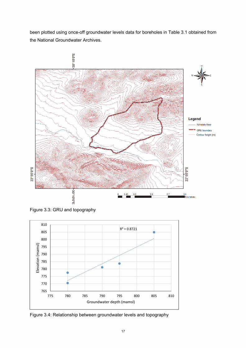
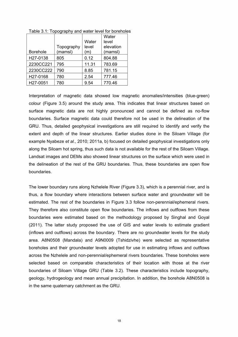
17

been plotted using once-off groundwater levels data for boreholes in Table 3.1 obtained from

the National Groundwater Archives.

Figure 3.3: GRU and topography

Figure 3.4: Relationship between groundwater levels and topography

R² = 0.8721

765

770

775

780

785

790

795

800

805

810

775 780 785 790 795 800 805 810

Elev

atio

n (m

amsl)

Groundwater depth (mamsl)

18

Table 3.1: Topography and water level for boreholes

Borehole Topography (mamsl)

Water level (m)

Water level elevation (mamsl)

H27-0138 805 0.12 804.88

2230CC221 795 11.31 783.69

2230CC222 790 8.85 781.15

H27-0168 780 2.54 777.46

H27-0051 780 9.54 770.46

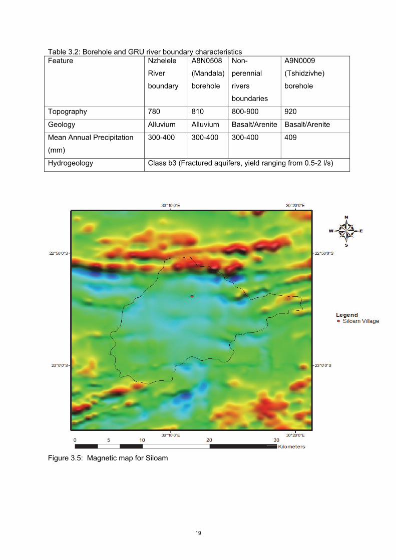
Interpretation of magnetic data showed low magnetic anomalies/intensities (blue-green)

colour (Figure 3.5) around the study area. This indicates that linear structures based on

surface magnetic data are not highly pronounced and cannot be defined as no-flow

boundaries. Surface magnetic data could therefore not be used in the delineation of the

GRU. Thus, detailed geophysical investigations are still required to identify and verify the

extent and depth of the linear structures. Earlier studies done in the Siloam Village (for

example Nyabeze et al., 2010; 2011a, b) focused on detailed geophysical investigations only

along the Siloam hot spring, thus such data is not available for the rest of the Siloam Village.

Landsat images and DEMs also showed linear structures on the surface which were used in

the delineation of the rest of the GRU boundaries. Thus, these boundaries are open flow

boundaries.

The lower boundary runs along Nzhelele River (Figure 3.3), which is a perennial river, and is

thus, a flow boundary where interactions between surface water and groundwater will be

estimated. The rest of the boundaries in Figure 3.3 follow non-perennial/ephemeral rivers.

They therefore also constitute open flow boundaries. The inflows and outflows from these

boundaries were estimated based on the methodology proposed by Singhal and Goyal

(2011). The latter study proposed the use of GIS and water levels to estimate gradient

(inflows and outflows) across the boundary. There are no groundwater levels for the study

area. A8N0508 (Mandala) and A9N0009 (Tshidzivhe) were selected as representative

boreholes and their groundwater levels adopted for use in estimating inflows and outflows

across the Nzhelele and non-perennial/ephemeral rivers boundaries. These boreholes were

selected based on comparable characteristics of their location with those at the river

boundaries of Siloam Village GRU (Table 3.2). These characteristics include topography,

geology, hydrogeology and mean annual precipitation. In addition, the borehole A8N0508 is

in the same quaternary catchment as the GRU.

19

Table 3.2: Borehole and GRU river boundary characteristics Feature Nzhelele

River

boundary

A8N0508

(Mandala)

borehole

Non-

perennial

rivers

boundaries

A9N0009

(Tshidzivhe)

borehole

Topography 780 810 800-900 920

Geology Alluvium Alluvium Basalt/Arenite Basalt/Arenite

Mean Annual Precipitation

(mm)

300-400 300-400 300-400 409

Hydrogeology Class b3 (Fractured aquifers, yield ranging from 0.5-2 l/s)

Figure 3.5: Magnetic map for Siloam

20

3.2 Hydrogeological conceptual model

A hydrogeological conceptual model is a pictorial presentation of the groundwater flow

system incorporating all available geological and hydrogeological data into a block diagram

or geological cross-section (Anderson and Woessner, 1992). Construction of a

hydrogeological conceptual model involves defining geological and hydrological frameworks

of the study area. Data for the geological framework is typically obtained from geological

maps, borehole logs, geophysics and additional field mapping (Wilson, 2005). Construction

of the geological framework then allows the hydrological framework to be defined involving

the following: (a) identifying the boundaries of the hydrological system, (b) defining

hydrostratigraphic units, (c) preparing a water budget, and (d) defining the flow system

(Sefelnasr, 2007).

Building a conceptual model is an iterative process that can identify gaps in the data, which

can be improved with further data gathering (Jackson, 2007). Thus, it is expected that there

will be continuous updating of the hydrogeological conceptual model of the study area as

more data becomes available.

3.2.1 Geology

• Regional geology

The study area falls within the younger covers of the Limpopo Mobile Belt (LMB). The LMB

(Figure 3.6) of southern Africa is an extensive high-grade terrain that can be subdivided into

three lithologically and structurally distinct zones, which are the northern marginal zone

(NMZ), central marginal zone (CMZ) and SMZ. The LMB was formed as a result of a

collision between the Kaapvaal craton (KC) and the Zimbabwe craton (ZC). The 250 km,

ENE-WNW trending LMB is thought to represent a Himalayan-style collision event between

the KC and ZC in the north (Bejaichund et al., 2009). The oblique nature of this collision is

believed to have initiated or re-activated major transcurrent fault systems, resulting in

important structures such as the Thabazimbi-Murchison lineament, which prepared the

craton for the development (2600-2100 million years ago) of the Transvaal and Griqualand

West basins (Singh et al., 2009).

Soutpansberg depositional basin was formed between two major crustal blocks, (e.g. the

Kaapvaal craton in the south and the Limpopo Belt in the north) as an east-west trending

asymmetrical rift or half-graben along the Palala Shear Belt (Brandl, 2003). Its rocks rest

21

unconformably on gneisses of the Limpopo Belt and Bandelierkop Complex. The Bumby et

al. (2002) suggested that the Soutpansberg Group may have been related to a half-graben

bound to the south by a northwards-dipping normal fault, perhaps associated with orogenic

collapse of the Limpopo Belt. The major faults which trend ENE through the Soutpansberg

region almost certainly represent reactivated basement fractures (Mason, 1973).

Figure 3.6: Simplified map of LMB (Chinoda et al., 2009)

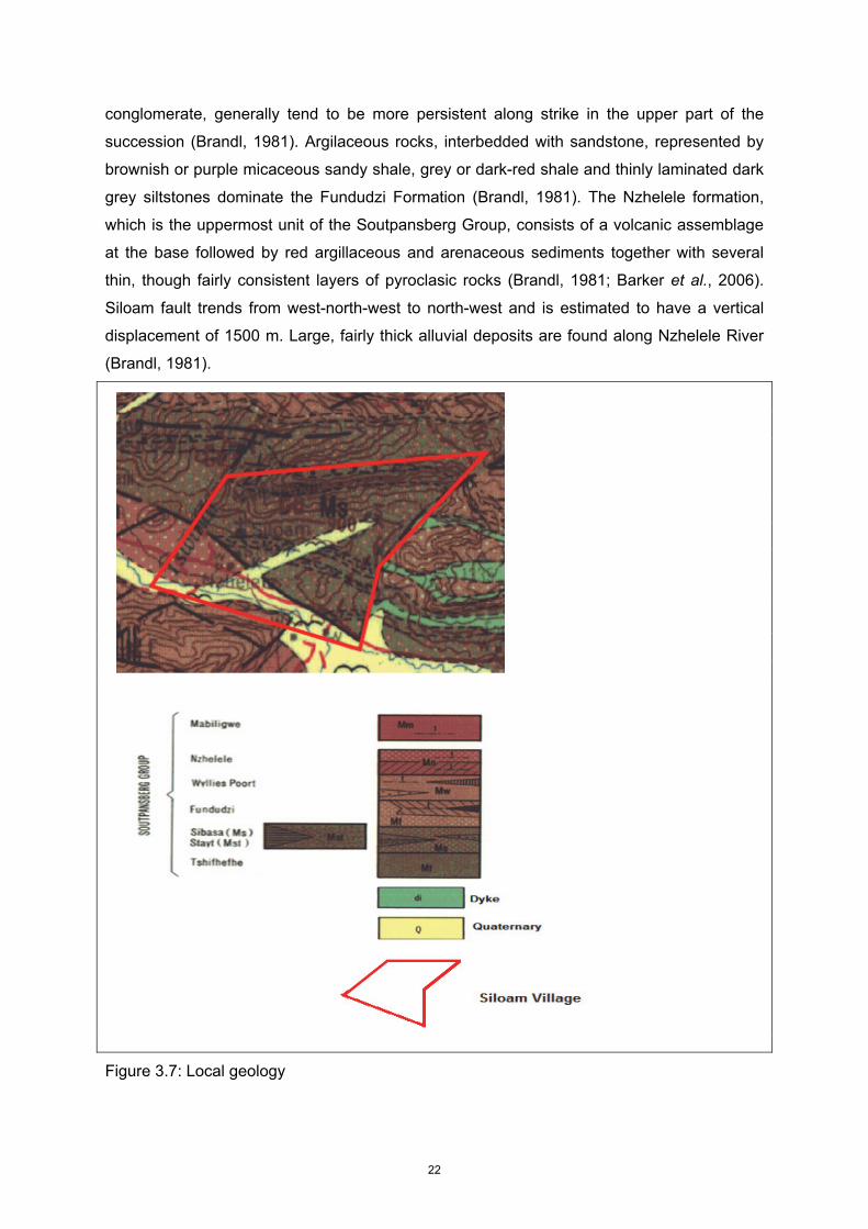
• Local geology

The study area falls within the severely faulted Soutpansberg Group of the Mokolian age

(Figure 3.7. The Soutpansberg Group emerges as a large east-west trending mountain

range (escarpment) from the Kruger National Park in the east to Vivo in the west. Dykes and

sills of diabase are plentiful in the Soutpansberg rocks (Brandl, 2003). It has 7 formations

which are Tshifhefhe, Sibasa Basalt, Fundudzi, Nzhelele, Wylliespoort, Stayt and

Mabalingwe (Figure 3.8). The Sibasa Basalt, Fundudzi and Nzhelele formations are the ones

that are present in the study area.

Sibasa formation consists predominantly of lava with minor intercalations of sedimentary and

tuffaceous rocks (Brandl, 1981). The volcanic rocks comprise of repetitive sequence of

erupted basalt (Barker et al., 2006). Sedimentary rocks, which include shale, quartzite and

22

conglomerate, generally tend to be more persistent along strike in the upper part of the

succession (Brandl, 1981). Argilaceous rocks, interbedded with sandstone, represented by

brownish or purple micaceous sandy shale, grey or dark-red shale and thinly laminated dark

grey siltstones dominate the Fundudzi Formation (Brandl, 1981). The Nzhelele formation,

which is the uppermost unit of the Soutpansberg Group, consists of a volcanic assemblage

at the base followed by red argillaceous and arenaceous sediments together with several

thin, though fairly consistent layers of pyroclasic rocks (Brandl, 1981; Barker et al., 2006).

Siloam fault trends from west-north-west to north-west and is estimated to have a vertical

displacement of 1500 m. Large, fairly thick alluvial deposits are found along Nzhelele River

(Brandl, 1981).

Figure 3.7: Local geology

23

Figure 3.8: Stratigraphy of the Soutpansberg Group in the western, central and eastern

Soutpansberg areas, and Blouberg area (Barker et al., 2006)

3.2.2 Geological cross-section and hydrogeological conceptual model

Figure 3.9 shows cross-section line C-D from which geologic cross-section was based. The

cross-section line was drawn on the map showing geologic formations of the study area.

This map has been extracted from the 1:250000 geologic map series for 2230 Messina. The

cross-section line C-D was selected because it is perpendicular to major geological

features/structures, and it cuts across the study area and the Nzhelele River. The geologic

formations include Sibasa Basalt, Fundudzi and Nzhelele formations and have been

described in sub-section 3.2.1. Figure 3.10 shows the geological cross-section C-D. A closer

24

observation on geological map shows that bedding dip to the north direction with 30, 27 and

20 degrees orientation (Figure 3.9).

The study area falls within the crystalline basement aquifers of the Limpopo Province.

Crystalline basement rocks are usually semi-confined (fractured bedrock) with water-table

aquifers (the matrix-regolith) situated on top of them (Holland, 2011). Wright (1992) stated

that basement aquifers have low permeability and the main groundwater flow systems are

relatively localised. In basement aquifers, groundwater occurs in secondary

porosity/fractures caused by weathering and fracturing (Adams et al., 2004). The main flow

paths in fractured rocks are along joints, fractures, shear zones, faults and other

discontinuities (Singhal and Gupta, 2010). Groundwater flow in fractured basement aquifers

is only possible along preferred pathways due to heterogeneity in their hydraulic properties

(for example, porosity and permeability) (Mohammed et al., 2015). Fractures serve as

primary sources that store and allow movement of water in hard rock areas (Sharma and

Baranwal, 2005). Since the study area falls within severely fractured Soutpansberg Group,

groundwater is likely to be stored in fractures and is expected to flow through preferential

pathways. Thus, groundwater flow mostly occurs through interconnected fractures.

25

Figure 3.9: Cross-section lines CD in the geological map

26

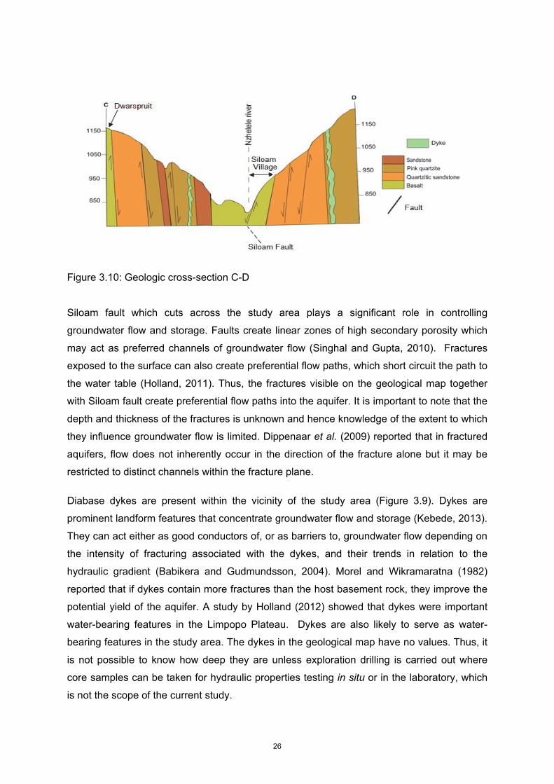
Figure 3.10: Geologic cross-section C-D

Siloam fault which cuts across the study area plays a significant role in controlling

groundwater flow and storage. Faults create linear zones of high secondary porosity which

may act as preferred channels of groundwater flow (Singhal and Gupta, 2010). Fractures

exposed to the surface can also create preferential flow paths, which short circuit the path to

the water table (Holland, 2011). Thus, the fractures visible on the geological map together

with Siloam fault create preferential flow paths into the aquifer. It is important to note that the

depth and thickness of the fractures is unknown and hence knowledge of the extent to which

they influence groundwater flow is limited. Dippenaar et al. (2009) reported that in fractured

aquifers, flow does not inherently occur in the direction of the fracture alone but it may be

restricted to distinct channels within the fracture plane.

Diabase dykes are present within the vicinity of the study area (Figure 3.9). Dykes are

prominent landform features that concentrate groundwater flow and storage (Kebede, 2013).

They can act either as good conductors of, or as barriers to, groundwater flow depending on

the intensity of fracturing associated with the dykes, and their trends in relation to the

hydraulic gradient (Babikera and Gudmundsson, 2004). Morel and Wikramaratna (1982)

reported that if dykes contain more fractures than the host basement rock, they improve the

potential yield of the aquifer. A study by Holland (2012) showed that dykes were important

water-bearing features in the Limpopo Plateau. Dykes are also likely to serve as water-

bearing features in the study area. The dykes in the geological map have no values. Thus, it

is not possible to know how deep they are unless exploration drilling is carried out where

core samples can be taken for hydraulic properties testing in situ or in the laboratory, which

is not the scope of the current study.

27

In the geological map (Figure 3.9), bedding planes, main fractures, dykes and the river trend

east-west (E-W). Since groundwater is expected to flow through the fractures, the

groundwater flow is likely to be from E-W. It is further conceptualised that groundwater flows

in and out of the GRU at open flow boundaries (non-perennial and Nzhelele Rivers),

depending on the hydraulic head. The inflows into the GRU constitute the recharge.

Additional recharge is from infiltration through the vadose zone. It is important to emphasise

that fracture network analysis and exploration drilling are required for detailed understanding

of the groundwater systems in the study area.

3.3 Aquifer characterisation

Pumping test data for 3 boreholes located within the study area were obtained from VSA

Leboa Consulting Pty Ltd. Drawdown versus logarithm of time (s vs log t), drawdown versus

time t in a log-log plot (log s vs. log t) and derivatives diagnostic plots were used to identify

and characterise flow regimes from constant discharge data. These plots were matched to

theoretical diagnostic plots to identify the aquifer type and characteristic flow regimes.

Theoretical diagnostic plots include Theis model infinite two-dimensional confined, double

porosity or unconfined, infinite linear no-flow boundary, infinite linear constant head

boundary, leaky aquifer, well-bore storage and skin effect, infinite conductivity vertical

fracture, general radial flow-noninteger flow dimension smaller than 2, general radial flow

model-non-integer flow dimension larger than 2, combined effect of well bore storage and

infinite linear constant head boundary. Detailed explanation of these diagnostic plots are

found in Kruseman and de Ridder (2000), Renard et al. (2009) and Holland (2011).

Comparison of diagnostic plots (s vs log t, log s vs. log t and their derivatives) for H27-0052,

H27-0138 and H27-0168 and theoretical diagnostic plots whose patterns matched those of

these boreholes is shown in Figure 3.11. The diagnostic plots for these boreholes were

constructed using AQTESOLV demo version. The theoretical diagnostic plots for variation 2

double porosity aquifer (Holland, 2011) are the ones that had patterns which are similar to

those of boreholes in the study area. Thus, the aquifer in the study area can be categorised

as a variation 2 double porosity type (Figure 3.11). The theoretical diagnostic plots for a

variation 2 double porosity aquifer in Figure 3.11s are from Holland (2011). According to

Holland (2011), the drawdown behaviour of this type of aquifer is characterised by distinct

dips (fracture dewatering) during late times of the associated derivative data and stepwise

drawdown.

28

Figure 3.11: Diagnostic plots for theoretical and study area boreholes

Theoretical Theoretical

H27-0138 H27-0138

H27-0052 H27-0052

H27-0168H27-0168

29

Two drawdown measurements of 10.35 m for borehole H27-0168 shows anomalous

behaviour as they deviated from the drawdown curve. Despite this, the aquifer is still

classified as a variation 2 double porosity aquifer due to distinct dips (fracture dewatering)

during late times of the derivative data. In a double porosity aquifer, matrix blocks have low

permeability and high (primary) porosity and storage capacity, only the fractures produce

flow directly to the well and matrix blocks act as a source, which feeds water into the

fractures (Holland, 2011). Renard et al. (2009) explained that early pumping depletes the

first reservoir (fractures, for example), which is then partly compensated by a delayed flux

provided by a second compartment of the aquifer (second/intermediate stage) and

equilibrium is reached at the late time (last stage). During the intermediate stage, drawdown

stabilises and the derivative shows a pronounced hole (dip) (Renard et al., 2009).

Kruseman and de Ridder (2000) categorised flow characteristics of double porosity aquifer

into three time periods, which are:

• Early pumping time, when all the flow comes from storage in the fractures

• Medium pumping time, a transition period during which the matrix blocks feed their

water at an increasing rate to the fractures, resulting in a (partly) stabilising

drawdown;

• Late pumping time, when the pumped water comes from storage in both the fractures

and the matrix blocks.

The flow regime characteristics described by Kruseman and de Ridder (2000) and Renard et

al. (2009) apply to the study area since it is characterised by double porosity aquifer. This

shows that the aquifer in the study area is also characterised by fracture dewatering.

Fracture dewatering has an effect on groundwater levels depending on the abstraction rate

(Van Tonder et al., 2002). Sarathchhandra and Jayawardena (1995) also associated drying

out of surface water resources to the dewatering cone extending along a linear rock fracture

in Sri Lanka. Fracture dewatering should be avoided, whenever possible, because of the

danger of mineral precipitation that can cause fracture and well clogging (Van Tonder et al.,

2002). The latter study noted that caution should be placed when assigning sustainable

yields to boreholes in aquifers characterised by fracture dewatering. This therefore means

that groundwater operating rules for aquifers characterised by fracture dewatering would aid

in minimising impacts associated with fracture dewatering since they regulate water

abstraction from the aquifer.

Pumping test data for 3 boreholes located within the study area obtained from VSA Leboa

Consulting Pty Ltd were analysed using Flow Characteristics (FC) method (Van Tonder

30

et al., 2001) to compute the aquifer characteristics (storativity and transmissivity). The details

of the boreholes and their locations are shown in Table 3.3. Table 3.4 shows the

transmissivity values for boreholes H27-0052, H27-0138 and H27-0168 computed using

Cooper Jacob method. They fall within the range of 1-24 m2/day determined by Holland

(2012) within the vicinity of the study areas. Storativity values could not be estimated based

on the methods used in the FC programme. This was because the methods used in the FC

programme are very insensitive to changes in drawdown and the calculated storativity

values are therefore biased (Dippenaar, 2008). The pumping test reports from VSA Leboa

Consulting (Pty) Ltd have reported storativity values of 0.0001 for all the boreholes listed in

Table 3.4. Figure 3.12 shows locations of the boreholes within the study area.

Table 3.3: Borehole details

Table 3.4: Transmissivity and yield

BH number T

(m2/day)

Recommended yield

(l/s)

Constant pumping

rate (yield) (l/s)

10 hour duty

cycle

24 hour

duty cycle

H27-0052 2.5 0.4 0.8 1.02

H27-0138 4.9 2.0 2.0 2.01

H27-0168 1.0 0.42 1.0 3.04

Storativity in confined aquifers fall within the range of 0.00005<S<0.005 and they indicate

that large pressure changes are required to produce substantial water yields (Todd and

Mays, 2005). Storage coefficient (storativity) is defined as the volume of water that an

aquifer releases from or takes into storage per unit surface area of the aquifer per unit

change in the component of head normal to that surface (Borrocu, 2014). Thus, the aquifer

in the study area is likely to store water in only 0.0001 (0.01 %) of its total storage volume.

Borehole

number

Latitude Longitude Altitude

(m)

Date of

test

H27-0052 30.190 22.301 805 1998/02/11

H27-0138 30.192 22.894 805 2003/02/14

H27-0168 30.188 22.904 780 1998/02/03

31

Figure 3.12: Boreholes locations Transmissivities, recommended yields and constant pumping rates (Table 3.4) for the

boreholes were mostly lower as compared to the average values of 514 boreholes which

had average values of 35.1 m2/day, 1.4 l/s, and 5.5 l/s, respectively, for similar aquifer type

(variation 2 double porosity), which were obtained in a study by Holland (2011). Low

transmissivity values indicate low rate of groundwater flow in the study area. It was only

borehole H27-0138 which had higher recommended yield of 2.0 l/s. The rest of the

32

boreholes had recommended yields which were lower than the average value of 1.4 l/s for

the 514 boreholes. Factors such as geology, rainfall, topography and thickness of

weathering are likely to cause variations in aquifer parameters.

33

4 DATA ACQUISITION

4.1 Preamble

This section presents data used for groundwater storage computation, groundwater storage-

reliability analysis and derivation of operating rules. This includes rainfall, evapotranspiration,

soil moisture, runoff, groundwater abstraction and groundwater quality data.

4.2 Rainfall, evapotranspiration and runoff

Patched rainfall data for station 0766324 for the period 1903/10/01-2000/07/31 (Figure 4.1)

was obtained from Lynch (2003). This was the only data available since the station was

closed in the year 2000. Rainfall and evapotranspiration for the period 2012-2013 (Figures

4.2 and 4.3, respectively) were obtained from the weather station installed at Siloam police

station in Siloam Village for the purpose of this research project. Extended

evapotranspiration data computed using the Hargreaves-Samani method for the period

1950-2000 (Figure 4.4) was obtained from Makungo (2009). The extension could only be

done for this period since it was the only period when temperature data was available.

Evaporation data for the period 2000-2012 was adopted from Mutshedzi weather station

which had data from 1991/07/01 to 2012/01/12. Evaporation data from Mutshedzi weather

station was used to compute evapotranspiration (Figure 4.5) for the period 2000-2012 based

on the pan evaporation method (Equation 4.1) described in Allen et al. (1998).

kEET P ×=0 (4.1)

ET0 is evapotranspiration, Ep is evaporation and k is the pan coefficient. The standard pan

coefficient of 0.7 was used. University of Venda weather station at Siloam Village and

Mutshedzi weather station are located in the same quaternary catchment (A80A) (Figure

4.6) and are expected to have similar hydrological behaviour. Runoff time series data for the

GRU (Figure 4.7) was simulated using Australian Water Balance Model. This model has

been selected because it achieved satisfactory to good model calibration and validation for

the same study area in a study by Makungo (2009).

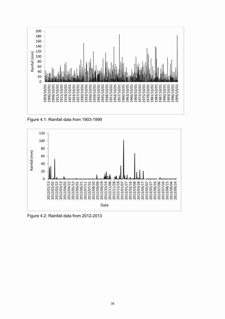
34

Figure 4.1: Rainfall data from 1903-1999

Figure 4.2: Rainfall data from 2012-2013

020406080

100120140160180200

1903

/10/

0119

06/1

0/01

1909

/10/

0119

12/1

0/01

1915

/10/

0119

18/1

0/01

1921

/10/

0119

24/1

0/01

1927

/10/

0119

30/1

0/01

1933

/10/

0119

36/1

0/01

1939

/10/

0119

42/1

0/01

1945

/10/

0119

48/1

0/01

1951

/10/

0119

54/1

0/01

1957

/10/

0119

60/1

0/01

1963

/10/

0119

66/1

0/01

1969

/10/

0119

72/1

0/01

1975

/10/

0119

78/1

0/01

1981

/10/

0119

84/1

0/01

1987

/10/

0119

90/1

0/01

1993

/10/

0119

96/1

0/01

1999

/10/

01

Rain

fall

(mm

)

0

20

40

60

80

100

120

2012

/01/

1320

12/0

2/02

2012

/02/

2220

12/0

3/13

2012

/04/

0220

12/0

4/22

2012

/05/

1220

12/0

6/01

2012

/06/

2120

12/0

7/11

2012

/07/

3120

12/0

8/20

2012

/09/

0920

12/0

9/29

2012

/10/

1920

12/1

1/08

2012

/11/

2820

12/1

2/18

2013

/01/

0720

13/0

1/27

2013

/02/

1620

13/0

3/08

2013

/03/

2820

13/0

4/17

2013

/05/

0720

13/0

5/27

2013

/06/

1620

13/0

7/06

2013

/07/

2620

13/0

8/15

2013

/09/

0420

13/0

9/24

Rain

fall

(mm

)

Date

35

Figure 4.3: Evapotranspiration data from 2012-2013

Figure 4.4: Evapotranspiration data from 1950-2000

Figure 4.5: Extended evapotranspiration data

0.001.002.003.004.005.006.007.008.009.00

2012

/01/

1320

12/0

2/02

2012

/02/

2220

12/0

3/13

2012

/04/

0220

12/0

4/22

2012

/05/

1220

12/0

6/01

2012

/06/

2120

12/0

7/11

2012

/07/

3120

12/0

8/20

2012

/09/

0920

12/0

9/29

2012

/10/

1920

12/1

1/08

2012

/11/

2820

12/1

2/18

2013

/01/

0720

13/0

1/27

2013

/02/

1620

13/0

3/08

2013

/03/

2820

13/0

4/17

2013

/05/

0720

13/0

5/27

2013

/06/

1620

13/0

7/06

2013

/07/

2620

13/0

8/15

2013

/09/

0420

13/0

9/24

Evap

otra

nspi

ratio

n (m

m/d

ay)

0.00

2.00

4.00

6.00

8.00

10.00

12.00

14.00

1950

/01/

01

1952

/01/

01

1954

/01/

01

1956

/01/

01

1958

/01/

01

1960

/01/

01

1962

/01/

01

1964

/01/

01

1966

/01/

01

1968

/01/

01

1970

/01/

01

1972

/01/

01

1974

/01/

01

1976

/01/

01

1978

/01/

01

1980

/01/

01

1982

/01/

01

1984

/01/

01

1986

/01/

01

1988

/01/

01

1990

/01/

01

1992

/01/

01

1994

/01/

01

1996

/01/

01

1998

/01/

01

2000

/01/

01

Evap

otra

spira

tion

(mm

/day

)

Date

0

2

4

6

8

10

12

14

2000

/01/

0120

00/0

6/01

2000

/11/

0120

01/0

4/01

2001

/09/

0120

02/0

2/01

2002

/07/

0120

02/1

2/01

2003

/05/

0120

03/1

0/01

2004

/03/

0120

04/0

8/01

2005

/01/

0120

05/0

6/01

2005

/11/

0120

06/0

4/01

2006

/09/

0120

07/0

2/01

2007

/07/

0120

07/1

2/01

2008

/05/

0120

08/1

0/01

2009

/03/

0120

09/0

8/01

2010

/01/

0120

10/0

6/01

2010

/11/

0120

11/0

4/01

2011

/09/

01

Evap

otra

nspi

ratio

n (m

m/d

ay)

Date

36

Figure 4.6: Location of Mutshedzi and University of Venda weather stations

Figure 4.7: Runoff data from 1980-2014

4.3 Soil moisture

The distribution of the soil moisture monitoring probes is shown in Figure 4.8. Due to the

rocky environment dominating the study area, it was not possible to install probes at some

locations. Five short (80 cm) and long (180 cm) probes for measuring soil moisture were

installed in Siloam Village in July 2011 and September 2012, respectively, to ensure

automatic and continuous monitoring of soil moisture. The probes were installed at 8 sites

and their identification numbers are given in Table 4.1. The 80 cm probes measured soil

0.000.501.001.502.002.503.003.504.004.505.00

1980

/01/

0119

81/0

1/01

1982

/01/

0119

83/0

1/01

1984

/01/

0119

85/0

1/01

1986

/01/

0119

87/0

1/01

1988

/01/

0119

89/0

1/01

1990

/01/

0119

91/0

1/01

1992

/01/

0119

93/0

1/01

1994

/01/

0119

95/0

1/01

1996

/01/

0119

97/0

1/01

1998

/01/

0119

99/0

1/01

2000

/01/

0120

01/0

1/01

2002

/01/

0120

03/0

1/01

2004

/01/

0120

05/0

1/01

2006

/01/

0120

07/0

1/01

2008

/01/

0120

09/0

1/01

2010

/01/

0120

11/0

1/01

2012

/01/

0120

13/0

1/01

2014

/01/

01

Runo

ff (m

3 /s)

Date

37

moisture at 10, 20, 30, 40, 60 and 80 cm depths while the 180 cm probes measured soil

moisture at 30, 60, 90, 120, 150 and 180 cm depths. Daily soil moisture data for some of the

probes for the periods July 2011-October 2013 and September 2012-October 2013 for short

and long probes is shown in Figures 4.8 and 4.9, respectively. Only data which was used for

soil moisture extension (at 80 and 180 cm depths) is presented in Figures 4.9 and 4.10.

Figure 4.8: Distribution of soil moisture probes

Figure 4.9: Soil moisture data for short probes

0102030405060708090

100

2011

/07/

1620

11/0

8/10

2011

/09/

0420

11/0

9/29

2011

/10/

2420

11/1

1/18

2011

/12/

1320

12/0

1/07

2012

/02/

0120

12/0

2/26

2012

/03/

2220

12/0

4/16

2012

/05/

1120

12/0

6/05

2012

/06/

3020

12/0

7/25

2012

/08/

1920

12/0

9/13

2012

/10/

0820

12/1

1/02

2012

/11/

2720

12/1

2/22

2013

/01/

1620

13/0

2/10

2013

/03/

0720

13/0

4/01

2013

/04/

2620

13/0

5/21

2013

/06/

1520

13/0

7/10

2013

/08/

0420

13/0

8/29

2013

/09/

2320

13/1

0/18

Soil

moi

stur

e (%

)

Date

17317 17433 1743717436 17438

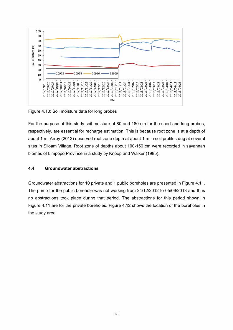
38

Figure 4.10: Soil moisture data for long probes

For the purpose of this study soil moisture at 80 and 180 cm for the short and long probes,

respectively, are essential for recharge estimation. This is because root zone is at a depth of

about 1 m. Arrey (2012) observed root zone depth at about 1 m in soil profiles dug at several

sites in Siloam Village. Root zone of depths about 100-150 cm were recorded in savannah

biomes of Limpopo Province in a study by Knoop and Walker (1985).

4.4 Groundwater abstractions

Groundwater abstractions for 10 private and 1 public boreholes are presented in Figure 4.11.

The pump for the public borehole was not working from 24/12/2012 to 05/06/2013 and thus

no abstractions took place during that period. The abstractions for this period shown in

Figure 4.11 are for the private boreholes. Figure 4.12 shows the location of the boreholes in

the study area.

0102030405060708090

100

2012

/09/

1320

12/0

9/20

2012

/09/

2720

12/1

0/04

2012

/10/

1120

12/1

0/18

2012

/10/

2520

12/1

1/01

2012

/11/

0820

12/1

1/15

2012

/11/

2220

12/1

1/29

2012

/12/

0620

12/1

2/13

2012

/12/

2020

12/1

2/27

2013

/01/

0320

13/0

1/10

2013

/01/

1720

13/0

1/24

2013

/01/

3120

13/0

2/07

2013

/02/

1420

13/0

2/21

2013

/02/

2820

13/0

3/07

2013

/03/

1420

13/0

3/21

2013

/03/

2820

13/0

4/04

2013

/04/

1120

13/0

4/18

2013

/04/

25

Soil

moi

stur

e (%

)

Date

20922 20918 20916 12669

39

Figure 4.11: Borehole abstractions

Figure 4.12: Location of boreholes

0

1

2

3

4

5

6

7

8

9

2011

/05/

2420

11/0

6/18

2011

/07/

1320

11/0

8/07

2011

/09/

0120

11/0

9/26

2011

/10/

2120

11/1

1/15

2011

/12/

1020

12/0

1/04

2012

/01/

2920

12/0

2/23

2012

/03/

1920

12/0

4/13

2012

/05/

0820

12/0

6/02

2012

/06/

2720

12/0

7/22

2012

/08/

1620

12/0

9/10

2012

/10/

0520

12/1

0/30

2012

/11/

2420

12/1

2/19

2013

/01/

1320

13/0

2/07

2013

/03/

0420

13/0

3/29

2013

/04/

2320

13/0

5/18

2013

/06/

1220

13/0

7/07

2013

/08/

0120

13/0

8/26

2013

/09/

20

Abst

ract

ions

(m3 /

day)

Date

40

4.5 Groundwater quality

Turbidity, EC and pH were measured for the period May 2011 to April 2012 for private and

public boreholes in the study area. Turbidity was measured using a calibrated Orion

AQUAfast II turbidity meter while the pH and electrical conductivity were measured using a

Multi 340i, Wissenschaftlich-Technische Werkstatten (WTW) multimeter. Additional data on

chemical water quality (of the boreholes for the period May-October 2011) was obtained

from Mafamadi (2012). Data on fluoride concentrations for the period August 2013 to

January 2014 was obtained from Mukhumo (2014). These had been analysed using Ion

Chromatography.

41

5 DATA EXTENSION: MODEL SET-UP, CALIBRATION AND VERIFICATION

5.1 Estimation of missing and extension of daily rainfall data using non-

parametric regression (NPR)

Non-parametric regression (NPR) has been used to estimate missing rainfall data for the

period 2000-2012. Regression analysis is often used in hydrology for exploring and

presenting relationships between variables (Adamowski, 1987) and to provide predictions of

unknown variables. NPR is one of the approaches used. It traces the dependence of a

response variable on one or several predictors without specifying in advance the function

that relates the predictors to the response (Fox, 2004). Non-parametric function estimation

refers to methods that strive to approximate a target function locally, i.e., using data from a

“small” neighbourhood of the point of estimate (Lall, 1995).

The general NPR model is written in a similar manner as linear regression, but the function f

is left unspecified (Fox, 2002). Non-parametric method is suitable for analysis of multimodal

distribution, which perhaps reflects more accurately the naturally occurring complex

hydrological cycle (Adamowski, 1987). Adamowski (1987) reported that simulation results of

studies by Adamoski (1985) and Labatiuk (1985) showed relative small values of bias and

root mean square error as compared to Log-Pearson type III when used for flood frequency

analysis. Lall (1995) gives the recent advances of application of NPR in hydrology. The

reviewed applications included frequency analysis, classification, spatial surface fitting, trend

analysis, time series forecasting and simulation of stochastic hydrology.

Non-parametric methods have also been applied in rainfall studies, though studies on

estimation of rainfall are limited. A non-parametric approach based on k-nearest neighbour

(KNN) estimator was used for spatial interpolation of rainfall data in a study by Ali (1998) and

was able to deal with non-stationary environment, irregular data, and site geometry. The

resulting statistics show a low estimation bias and a high variance. Kalra and Ahmad (2011)

estimated seasonal precipitation by disaggregating water year precipitation for 29 climate

divisions in the Colorado River Basin using a KNN non-parametric technique. The results

indicated satisfactory estimation of seasonal precipitation during winter and spring seasons

compared to autumn and summer seasons. The latter study also showed superiority of KNN

approach when compared to a first-order periodic autoregressive parametric approach.

Sharma and Lall (1999) used a non-parametric model to simulate daily rainfall spells and

amounts in Sydney, Australia. The model was able to accurately represent non-stationarity

42

of the rainfall generation mechanism and the seasonal characteristics of the observed

rainfall. The study noted that the use of non-parametric methods enables accurate

representation of the distributional features that characterise rainfall. The current review did

not find any related studies that have been done in South Africa.

Other applications of non-parametric techniques in rainfall studies include development of

nonparametric seasonal wet/dry spell stochastic model for resampling daily precipitation (Lall

et al., 1996), and stochastic generation of rainfall data (Rajagopalan and Lall, 1999; Harrold,

2002; Harrold et al., 2003; Srikanthan et al., 2005).

5.1.1 NPR modelling methodology

Daily rainfall data for Mutshedzi rainfall station was available for the period 1991/07/01 to

2012. This rainfall data was obtained from the Department of Water Affairs. It was essential

to estimate rainfall data for Siloam weather station for the period 2000/08/01 to 2012/01/12

since it is one of the inputs into the groundwater balance. Rainfall for Mutshedzi and Siloam

weather stations were used as inputs and outputs of the NPR model, respectively.

Daily rainfall data for the period 1991/07/01 to 2000/07/31 was used to calibrate and validate

the non-parametric model since it was the period when data for the two stations was

available. 60% (1991) and 40% (1328) data points were used for calibration and validation,

respectively. These were the percentages that gave the best model performance after

several trial runs. The data points used for calibration and validation were randomly selected

by the model.

Daily rainfall data for Mutshedzi weather station for the period 2000/08/01 to 2012/01/12 was

used to estimate rainfall data for Siloam weather station for the same period. Robust locally

weighted scatter smoother (LOWESS) NPR method with kernel (tricube) weighting function

(Equation 5.1) and two polynomial degrees was selected for this study. This method was

selected because it gave the best results after running several trials using other non-

parametric regression methods weighting functions.

( )= <−

≥1110

33

)( zforz

zforT zW (5.1)

( )i

ii h

xxz 0−=

43

zi is the scaled distance between the predictor value for the ith observation and x is the focal;

hi is the band width of the local regression centered on xi.

Robust LOWESS was used to fit local polynomial regressions for all the estimation points

and to join them together. This involved weighting each neighbouring data point according to

a kernel weighting function, which assigns decreasing weight with distance from the point of

estimation and then computes a weighted local polynomial regression model. Further details

on robust LOWESS fitting procedure are found in Cleveland (1979) and Cleveland and

Devlin (1988). The computations were automatically done in XLSTAT, which is an add-in

component of Excel Spreadsheet. In general, the computations were according to the

following steps:

• A fitting step where the best combination of model type, kernel weighting function,

and bandwidth are obtained using the test sample;

• A validation phase that allows validation of the model on new observations;

• An application phase, where the model is applied to a new set of data to estimate the

unknown variable.

The performance of the model was evaluated based on root mean square error (RMSE),

mean square error (MSE), mean bias (BIAS), correlation coefficient (R) and coefficient of

determination (R2) (Equations 5.2-5.6).

44

(5.2)

( )=

−=n

iii PO

nMSE

1

21 (5.3)

( )=

−=n

iii PO

nBIAS

1

1 (5.4)

(5.5)

(5.6)

where Oi = observed rainfall (mm), Pi = estimated rainfall (mm), i= number of the day, n =

total number of time steps and iP is the mean rainfall.

RMSE and MSE are valuable because they indicate errors of the constituent of interest,

which aids in analysis of the results (Moriasi et al., 2007). RMSE gives an idea of the

absolute differences between observed and modelled values in their original units of

measurement (Hyndman and Koehler, 2006). R and R2 describe the degree of co-linearity

between simulated and measured data (Moriasi et al., 2007; Obiero et al., 2011). The

coefficient of determination determines the proportion of in-situ variance that can be

explained by the model (Rathjens and Oppelt, 2012). Bias measures the average tendency

of the simulated constituent values to be larger or smaller than the measured data (Moriasi

et al., 2007).

5.1.2 NPR modelling results

The comparisons of observed and estimated rainfall for calibration and validation runs

(Figures 5.1 and 5.2, respectively) show a general agreement between observed and

simulated rainfall. A general visual agreement between observed and simulated constituent

( ) 21

1

21

−= =

n

iii PO

nRMSE

( )( )

( ) ( )

−−

−−=

= =

=

n

i

n

iiiii

n

iiiii

PPPP

POPOR

1 1

22

1

( )( )

( ) ( )

2

1 1

22

12

−−

−−=

= =

=

n

i

n

iiiii

n

iiiii

PPPP

POPOR

45

data indicates adequate calibration and validation over the range of the constituent being

simulated (Singh et al., 2004). LOWESS model was able to estimate low rainfall values for

both calibration and validation runs relatively well. Peak rainfall events were mostly

underestimated in both calibration and validation runs. For example, high peak rainfall

events (> 40 mm) for the days 19 February 1995, 16 February 1996, and 06 February 2000

(Figure 5.1), and 18 February 1995, 11 January 1996 and 22 February 2000 (Figure 5.2)

were underestimated in calibration and validation runs, respectively. Simolo (2010) reported

that underestimation of intense precipitation events is a typical side effect of regression-

based approaches. Ali (1998) also found that NPR approach failed to estimate the extreme

rainfall values due to over smoothing.

Figure 5.1: Observed and estimated rainfall for calibration run for stations

Figure 5.2: Observed and estimated rainfall for validation run for stations

Table 5.1 shows the performance measures for calibration and validation runs together with

their acceptable ranges. RMSE and BIAS values for both the calibration and the validation

020406080

100120140160180200

1991

/07/

0419

91/1

0/15

1992

/01/

2519

92/0

5/06

1992

/08/

1719

92/1

1/29

1993

/02/

2519

93/0

6/19

1993

/09/

2419

94/0

1/03

1994

/04/

1019

94/0

7/20

1994

/10/

2819

95/0

2/02

1995

/05/

1419

95/0

8/10

1995

/11/

1819

96/0

2/21

1996

/06/

1619

96/1

0/08

1997

/01/

1919

97/0

4/22

1997

/08/

0519

97/1

1/20

1998

/03/

0819

98/0

6/09

1998

/09/

2819

99/0

1/09

1999

/03/

2819

99/0

6/24

1999

/09/

2919

99/1

2/30

2000

/04/

1620

00/0

7/12

Ranf

all (

mm

)

Date

Estimated

Observed

0

20

40

60

80

100

120

140

1991

/07/

0119

00/0

3/30

1900

/07/

1519

00/1

0/27

1901

/01/

3119

01/0

5/01

1901

/08/

3119

01/1

1/28

1902

/03/

0519

02/0

6/26

1902

/09/

2819

03/0

1/13

1903

/04/

2319

03/0

8/07

1903

/11/

2219

04/0

3/21

1904

/06/

2819

04/1

0/10

1905

/01/

0419

05/0

3/18

1905

/07/

0719

05/1

0/21

1906

/01/

3019

06/0

4/25

1906

/07/

3119

06/1

1/14

1907

/02/

1319

07/0

5/12

1907

/10/

0519

08/0

1/25

1908

/05/

2419

08/0

9/09

1908

/12/

25

Rain

fall

(mm

)

Date

Observed Estimated

46

(Table 5.1) are reasonable as they are low and fall within the ranges obtained in other

studies. RMSE of 64 mm was obtained in a study by Ali (1998). Kalra and Ahmad (2011)

obtained RMSE values ranging from 0.44 to 2.69 inches, which are equivalent to a range of

11.18 to 68.33 mm. The relatively low computed BIAS values for calibration and validation

show minimal estimation errors. These are lower than BIAS value of 7 mm, which was

obtained in a study by Ali (1998). R values for calibration and validation exceed 0.8 showing

satisfactory model performance. R2 values exceed the acceptable value of 0.5 showing

acceptable model performance. The model showed acceptable and satisfactory performance

based on the assessed measures of performance. Thus, the model can effectively estimate

missing rainfall for Siloam station. The estimated rainfall for Siloam Village is shown in

Figure 5.3.

Table 5.1: Performance measures for calibration and validation runs

aShamsudin and Hashim (2002); bElshamy (2008), cVan Liew et al. (2007); dSingh et al.

(2004)

Figure 5.3: Estimated rainfall for Siloam Village

5.2 Extension of soil moisture data

A modelling code coupling a linear and a non-linear system identification models was used

in the extension of soil moisture data. The code has the same structure as the one used in

05

101520253035

2000

/08/

0120

00/1

2/01

2001

/04/

0120

01/0

8/01

2001

/12/

0120

02/0

4/01

2002

/08/

0120

02/1

2/01

2003

/04/

0120

03/0

8/01

2003

/12/

0120

04/0

4/01

2004

/08/

0120

04/1

2/01

2005

/04/

0120

05/0

8/01

2005

/12/

0120

06/0

4/01

2006

/08/

0120

06/1

2/01

2007

/04/

0120

07/0

8/01

2007

/12/

0120

08/0

4/01

2008

/08/

0120

08/1

2/01

2009

/04/

0120

09/0

8/01

2009

/12/

0120

10/0

4/01

2010

/08/

0120

10/1

2/01

2011

/04/

0120

11/0

8/01

2011

/12/

01

Estim

ated

rain

fall

(mm

)

Date

Performance

Measure Calibration Validation

Acceptable ranges

RMSE (mm) 3.67 3.03 0 = Perfecta

BIAS (mm) 0.53 0.4 0 = Perfectb

R 0.87 0.84

>0.5 – Acceptablec;

≥0.80 – satisfactoryd

MSE (mm) 13.48 9.19 0 = Perfectc

R2 0.76 0.7 >0.5 – Acceptableb

47

extension of groundwater levels. Within, the developed modelling code, a linear polynomial

model is used to initialise the non-linear Hammerstein-Wiener model. The polynomial has

model orders of number of past output terms used to predict current output (na), number of

past input terms used to predict current output (nb) and delay from input to output in terms of

number of samples (nk), and Output-Error (OE) model structure. The initialisation configures

the non-linear Hammerstein-Wiener model to use orders and delays of the linear model, and

polynomials as the transfer functions (Ljung, 2014). This initialisation aids in improving the fit

of the model. OE model structure is one of the various linear model structures that provide

different ways of parameterising the transfer functions of linear input-output polynomial

model within system identification software (Ljung, 2014).

Hammerstein-Wiener models describe dynamic systems using one or two static nonlinear

blocks in series with a linear block. Detailed description of these models is provided in Ljung

(2014). Selected model orders for each probe are shown in Table 5.2. These model orders

were selected because they gave the best results after several trial runs. Although

monitored soil moisture data was available for 5 probes, only 3 could be used for modelling

and extension. This was because two of the probes had a lot of gaps that could not be

patched.

Table 5.2: System model orders Probe Model orders (na, nb, nk)

used

20918 1,1; 4,4; 1,1

20922 4,4; 4,4; 3,3

12699 2,2;1,1;1,1

Figures 5.4-5.6 show observed and estimated soil moisture for calibration and validation

runs. The comparisons of observed and estimated soil moisture for calibration and validation

runs show agreement between observed and simulated soil moisture. Measures of

performance (Table 5.3), which are within acceptable ranges support this. Extended soil

moisture data is presented in Figure 5.4.

48

Figure 5.4: Observed and estimated soil moisture for calibration and validation runs for probe 12699

Figure 5.5: Observed and estimated soil moisture for calibration and validation runs for probe 20918

Figure 5.6: Observed and estimated soil moisture for calibration and validation runs for probe 20922

Calibration

49

Table 5.3: Computed measures of performance and their acceptable ranges

aShamsudin and Hassim (2002); bElshamy (2008), cVan Liew et al. (2007); dSingh et al.

2004

Figure 5.7: Extended soil moisture

505560657075808590

1980

/10/

0519

81/1

0/05

1982

/10/

0519

83/1

0/05

1984

/10/

0519

85/1

0/05

1986

/10/

0519

87/1

0/05

1988

/10/

0519

89/1

0/05

1990

/10/

0519

91/1

0/05

1992

/10/

0519

93/1

0/05

1994

/10/

0519

95/1

0/05

1996

/10/

0519

97/1

0/05

1998

/10/

0519

99/1

0/05

2000

/10/

0520

01/1

0/05

2002

/10/

0520

03/1

0/05

2004

/10/

0520

05/1

0/05

2006

/10/

0520

07/1

0/05

2008

/10/

0520

09/1

0/05

2010

/10/

0520

11/1

0/05

2012

/10/

0520

13/1

0/05

Soil

moi

stur

e (%

)

Date

Performance Measure

12699 20922 20918 Acceptable values

Cal Val Cal Val Cal Val Coefficient of determination (R2)

0.993 0.93 0.90 0.95 0.96 0.71 >0.5 – Acceptableb

Correlation coefficient (R) 0.996 0.87 0.95 0.97 0.98 0.81 >0.5 – Acceptablec; ≥ 0.80 – satisfactoryd

RMSE (%) 0.31 1.38 1.23 2.38 0.18 0.18 0 = Perfecta MSE (%) 0.51 1.90 1.50 5.70 0.42 0.43 0 = Perfecta

50

6 GROUNDWATER STORAGE-RELIABILITY ANALYSIS AND OPERATING

RULES

6.1 Groundwater storage-reliability analysis

Though the study had proposed groundwater yield-reliability analysis for the purpose of

developing groundwater operating rules, this was not possible due to lack of long-term time

series of groundwater yield data in the study area. Groundwater storage-reliability analysis

was used as an alternative approach that made it possible to develop groundwater operating

rules. Groundwater storage-reliability analysis involved the computation of weekly

groundwater storages and their reliability. Computation of groundwater storage time series

was done following the hydrological year (October of a given year to September of the

following year). The weekly change in groundwater storage time series was computed using

the groundwater balance (Equation 6.1).

GQQsETRP aioo Δ±=−±Δ±−− (6.1)

where P= precipitation, Ro= runoff, ET= evapotranspiration, ∆s= change in soil water

storage, Qio= inflow/outflow at open flow boundaries, Qa = groundwater abstraction and GΔ= change in groundwater storage. The runoff component of the equation is comprised of

both storm runoff and baseflow and thus, accounts for groundwater loss into the river during

the dry season. Groundwater storage was computed at a weekly scale since it was

envisaged that there would be no significant difference in groundwater storage at a daily

scale. Weekly groundwater storage time series was computed from Equation 6.2.

GGG tt Δ±=+1 (6.2)

Gt and Gt+1 are the storages at periods t and t+1, respectively. Gt was estimated by

computing the total storage volume of the groundwater reservoir (GTotal) using Equation 6.3.

This was used to compute groundwater storage time series, assuming that the groundwater

reservoir was at full storage level (100% saturation) at the beginning of the analysis (i.e. at

time, t). To account for possible variations in groundwater storage at time, t, groundwater

storage time series was also computed for scenarios assuming 80, 60, 40, 30, 25, 20 and

10% of full groundwater reservoir storage level (GRSL). Groundwater storage reservoir has

been used in this study to refer to the portion of the GRU where groundwater is stored in

interconnected fractures, faults, cracks and/or openings in the aquifer.

51

ShAGTotal ××= (6.3)

Where A= area of the GRU, h=saturated thickness of the aquifer and S= storativity. There

were no values of saturated aquifer thickness from the pumping test data for the 3 boreholes

in the study area. However, most of South Africa’s accessible groundwater is stored in the

upper fractured and weathered zone whose saturated thickness was found to be 25 m

(Vegter, 1995). This value is closer to the maximum drawdown of 25.6 m from pumping test

data for borehole H27-0138 (Figure 3.11). The maximum drawdowns from pumping test data

for boreholes H27-0052, H27-0168 and H27-0138 (Figure 3.11), which are 17.23, 19.1 and

25.6 m, respectively, would indicate variable average saturated aquifers thicknesses. Since

drawdown levels data could only be obtained from 3 boreholes, it was considered

appropriate to adopt the average saturated thickness of 25 m from Vegter (1995), which

would be more representative of the average spatial saturated thickness of the aquifer in the

study area.

Values for each week of the year from October 1980 to September 2013 were extracted

from the computed groundwater storage time series such that 52 data sets, each with 33

data points for each storage scenario, were generated. These were ranked in ascending

order and their reliability was calculated using Weibull plotting position formula (Equation

6.4).

1+=n

mp (6.4)

p is the probability that the magnitude ranked m is exceeded for a ranked series that is n

years long. The reliability associated with the magnitude ranked m was obtained as reliability

= 100p% following Ndiritu et al. (2011a). Figure 6.1 shows the computed groundwater

storage for the period 1980-2013 for 100% of GRSL. This represents the volume of water

stored within the GRU. The flood which occurred in the 1996/97 hydrological year

contributed to a rise in groundwater storage, which was continuously maintained by the

1999/2000 and subsequent hydrological year floods. The other floods include 2010/2011

and 2012/2013, though they were of lower magnitude as compared to the 1999/2000 flood.

This explains generally higher groundwater storage after the year 1996 as compared to the

years before.

52

Figure 6.1: Computed groundwater storage time series at full storage level

Examples of groundwater storage-reliability curves for selected weeks of the year at 10, 20,

40, 60, 80 and 100% of GRSLs are shown in Figure 6.2. These have been extracted from

Appendix A. The curves show groundwater storages available at different reliabilities within

specific weeks and they form the basis of deriving groundwater operating rules, since they

give an indication of storages, which would ensure adequate supply of groundwater. The

dates that fall within each specific week are in Table 6.1. Weeks 1, 10, 20, 30, 40 and 50

covers the weeks starting on the dates of 1980/10/06, 1980/12/07, 1981/02/15, 1981/04/26,

1981/07/05 and 1980/09/13 (Table 6.1). These have been used to represent the weeks,

which fall in the wet and dry rainfall seasons. This is useful when assessing the availability of

groundwater throughout the year.

Relatively high and low storages are associated with low and high levels of reliability,

respectively. For example, storages with 10% reliability are higher than those with 98%

reliability. This is because high storages are a result of heavy rainfall events which rarely

occur as compared to normal rainfall events. Thus, the reliability of such high rainfall events

is generally low. However, in terms of groundwater storage, such rainfall events are

significant since they significantly increase the groundwater storage, which may be available

for use during dry periods. Thus, heavy rainfall events contribute to major recharge events.

Van Wyk et al. (2012) reported that episodic rainfall events are responsible for rapid, but

sustainable groundwater recharge events in semi-arid areas of South Africa.

Since, the risk (R) of failure of a water supply source is calculated as pR −= 1 , where p is

the reliability, storages with low and high levels of reliability, are thus associated with high

and low risk of failures, respectively. This therefore means that groundwater storages with

high levels of reliability are the ones that can ensure continuous and adequate supply with

15000

16000

17000

18000

19000

20000

21000

1980

/10/

0519

81/1

0/05

1982

/10/

0519

83/1

0/05

1984

/10/

0519

85/1

0/05

1986

/10/

0519

87/1

0/05

1988

/10/

0519

89/1

0/05

1990

/10/

0519

91/1

0/05

1992

/10/

0519

93/1

0/05

1994

/10/

0519

95/1

0/05

1996

/10/

0519

97/1

0/05

1998

/10/

0519

99/1

0/05

2000

/10/

0520

01/1

0/05

2002

/10/

0520

03/1

0/05

2004

/10/

0520

05/1

0/05

2006

/10/

0520

07/1

0/05

2008

/10/

0520

09/1

0/05

2010

/10/

0520

11/1

0/05

2012

/10/

0520

13/1

0/05

Grou

ndw

ater

stot

rage

(m3 )

53

low risk of failure. The volume of water in storage increases as the percentage storage

volume increases, hence 100% storage has highest storage volumes (Figure 6.2).

Figure 6.2: Weekly groundwater storage-reliability curves

10% storage

40% storage 60% storage

80% storage 100% storage

20%

54

Table 6.1: Weekly start and end dates Week Start date End date Week Start date End date

1 1980/10/06 2012/10/07 27 1981/04/05 2013/04/07

2 1980/10/12 2012/10/14 28 1981/04/12 2013/04/14

3 1980/10/19 2012/10/21 29 1981/04/19 2013/04/21

4 1980/10/26 2012/10/28 30 1981/04/26 2013/04/28

5 1980/11/02 2012/11/04 31 1981/05/03 2013/05/05

6 1980/11/09 2012/11/11 32 1981/05/10 2013/05/12

7 1980/11/16 2012/11/18 33 1981/05/17 2013/05/19

8 1980/11/23 2012/11/25 34 1981/05/24 2013/05/26

9 1980/11/30 2012/12/02 35 1981/05/31 2013/06/02

10 1980/12/07 2012/12/09 36 1981/06/07 2013/06/09

11 1980/12/14 2012/12/16 37 1981/06/14 2013/06/16

12 1980/12/21 2012/12/23 38 1981/06/21 2013/06/23

13 1980/12/28 2012/12/30 39 1981/06/28 2013/06/30

14 1981/01/04 2013/01/06 40 1981/07/05 2013/07/07

15 1981/01/11 2013/01/13 41 1981/07/12 2013/07/14

16 1981/01/18 2013/01/20 42 1981/07/19 2013/07/21

17 1981/01/25 2013/01/27 43 1981/07/26 2013/07/28

18 1981/02/01 2013/02/03 44 1981/08/02 2013/08/04

19 1981/02/08 2013/02/10 45 1981/08/09 2013/08/11

20 1981/02/15 2013/02/17 46 1981/08/16 2013/08/18

21 1981/02/22 2013/02/24 47 1981/08/23 2013/08/25

22 1981/03/01 2013/03/03 48 1981/08/30 2013/09/01

23 1981/03/08 2013/03/10 49 1981/09/06 2013/09/08

24 1981/03/15 2013/03/17 50 1981/09/13 2013/09/15

25 1981/03/22 2013/03/24 51 1981/09/20 2013/09/22

26 1981/03/29 2013/03/31 52 1981/09/27 2013/09/29

6.2 Groundwater quality assessment

The measured pH, turbidity and EC values from May 2011 to April 2012 are shown in Table

6.2. Two of the sampled boreholes (Communal and Hot spring) had pH values which were a

slightly higher than DWAF (1996) water quality guideline for domestic use of 6-9 in the

months of October 2011, and September and December 2011, respectively. These pH

values do not have any potential health effects but only have a slight soapy taste in drinking

water and insignificant effects on bathing. Turbidity values for most of the boreholes were

generally higher than 1 NTU provided in the DWAF (1996) guideline. Thus, there is a slight

risk of potential health effects caused by turbidity as stated in DWAF et al. (1998) in most

boreholes. Incomplete borehole development such as lack of installations of screens in

boreholes drilled in hard rock aquifers contributes to disintegrated rock particles or eroded

sediments increasing turbidity levels. Three of the sampled boreholes (Community, Hot

55

spring and Project) had EC values within the guideline of less than 70 mS/m. Siphali, Siaga,

Gemeli, Manenzhe, Musekwa and Luvhimbi boreholes had EC values ranging from 208 to

2070 mS/m. Effects of these high EC values include distinct and extreme salty and bitter

taste in water, slight possibility of salt overloading in sensitive groups, corrosion in laundry,

impaired soap lathering and increasing risk of dehydration. However, for Siphoro,

Mugagadeli and Tawanda boreholes, EC varies from 4 to 125 mS/m, that is, from

acceptable to unacceptable values.

Analysed non-metals in groundwater from sampled boreholes are shown in Figure 6.3. Most

boreholes had fluoride (F) concentrations, which were far much higher than the DWAF

(1996) guideline of 1.5 mg/L (Figure 6.3). Effects associated with these concentrations are

severe tooth staining from drinking water and increased risk of health effects from food

preparation. A survey by Odiyo et al. (2012) revealed that 85% of family members from 87%

of households that use groundwater have mottled teeth due to high fluoride concentrations in

groundwater. 50% of children between the ages of 11 and 14 in Siloam Primary School also

had mottled teeth (Odiyo et al., 2012). Most boreholes had chloride concentrations

exceeding the DWAF (1996) guideline of <100 mg/L. Effects of such concentrations include

possible long-term health effects for cooking and drinking, objectionable salty taste and

corrosion in laundry. Siphali is the only borehole that had high sulphate (SO4)

concentrations exceeding DWAF (1996) water quality guideline in the months of May and

October 2012. The concentrations are associated with possible slight corrosion of laundry

but suitable for all the other domestic uses. All boreholes had nitrate concentrations, which

were less than DWAF (1996) guideline of <26 mg/L. Water from a few boreholes exceeded

the SABS 241 (1996) guideline for phosphate (PO4) in drinking water of 15 mg/L.

56

Table 6.2: Turbidity, EC and pH values

TURBIDITY

DATE COM HSP SI SO MG PT TA SA MAN MUS LI GE

May-11 0.7 4.4 0.5 2.9 0.2 0.2 1.2 0.3 2.2 11.5 4.2 7.4

Jun-11 5.6 4.3 0.3 3.4 0.6 0.1 0.1 2.1 0.9 6.3 6.0 7.0

Jul-11 4.1 1.2 2.9 2.0 9.7 1.3 1.6 0.1 1.9 2.3 8.3 9.4

Aug-11 2.0 4.4 3.5 2.7 4.5 0.2 3.4 0.5 1.0 0.1 10.1 10.3

Sep-11 2.3 1.8 2.3 2.3 3.0 2.0 1.9 1.1 2.3 1.0 12.5 4.3

Oct-11 0.7 1.5 3.4 2.6 3.8 0.4 1.6 0.2 2.2 1.9 9.1 9.9

Nov-11 5.0 4.3 1.9 1.5 1.7 7.7 6.9 3.6 5.4 1.1 3.8 3.6

Dec-11 5.7 0.2 6.5 5.8 2.8 4.5 Nm 4.6 4.7 4.2 5.9 4.6

Jan-12 4.6 4.9 6.2 5.1 1.9 1.4 4.0 5.2 5.1 3.4 7.8 5.2

Feb-12 13.3 7.9 10 8.1 10.6 15.5 11.3 13 10.3 16.5 11 13

Mar-12 2.2 2.0 2.5 1.9 0.01 Nm 6.8 2.8 3.0 2.3 2.9 0.3

Apr-12 nm 2.2 2.1 2.1 2.2 2.0 nm 2.3 2.1 3.2 0.8 2.0

pH

DATE COM HSP SI SO MG PT TA SA MAN MUS LI GE

May-11 7.6 8.8 7.6 7.6 8.1 7.9 7.2 7.7 7.6 8.3 8.0 7.7

Jun-11 8.6 8.3 8.0 7.7 8.1 7.7 7.4 7.9 7.7 8.6 8.0 7.6

Jul-11 8.6 8.9 7.7 8.0 8.2 7.8 7.1 7.9 7.8 8.6 7.9 7.3

Aug-11 8.9 9.0 7.4 8.0 8.4 8.5 7.4 7.9 7.5 8.7 7.9 7.9

Sep-11 9.0 9.1 7.0 7.5 9.0 8.4 7.1 7.5 7.6 8.8 8.1 7.4

Oct-11 9.1 9.0 7.1 7.3 8.7 8.6 7.1 7.5 7.6 8.7 8.3 7.1

Nov-11 8.3 9.0 7.5 7.6 7.6 8.2 7.7 7.6 7.5 8.2 8.4 7.2

Dec-11 9.0 9.1 7.4 8.3 8.5 8.1 nm 7.91 7.5 8.7 8.0 7.4

Jan-12 8.7 8.9 7.3 8.3 8.5 8.0 7.11 7.47 7.5 8.7 8.3 7.1

Feb-12 8.9 8.8 6.9 7.0 7.8 8.0 7.54 6.99 7.1 8.5 7.5 6.9

Mar-12 6.7 6.8 6.8 6.8 6.8 Nm 6.74 6.83 6.8 6.8 6.7 nm

Apr-12 6.7 6.7 6.7 6.7 6.7 6.6 6.67 6.7 6.7 6.7 6.7 6.7

EC

DATE COM HSP SI SO MG PT TA SA MAN MUS LI GE

May-11 37.7 32.8 224.0 104.7 48.9 37.1 4.0 1769.0 1926.0 763.0 1324.0 1899.0

Jun-11 34.3 32.8 221.0 115.7 69.8 37.6 4.1 1662.0 1887.0 740.0 1028.0 2070.0

Jul-11 33.8 33.5 222.0 122.9 83.0 37.5 54.3 1641.0 1953.0 739.0 1163.0 2020.0

Aug-11 33.5 33.3 218.0 124.6 62.3 40.5 56.1 1722.0 1981.0 741.0 1017.0 1934.0

Sep-11 34.9 33.3 240.0 125.1 37.3 41.7 60.4 1721.0 1940.0 136.0 1166.0 2050.0

Oct-11 33.9 33.3 258.0 125.0 48.6 39.7 80.6 1653.0 1884.0 750.0 1172.0 2050.0

Nov-11 33.0 32.7 247.0 12.2 64.8 41.6 76.2 1110.0 1228.0 362.0 695.0 1237.0

Dec-11 33.3 32.7 208.0 12.0 44.8 41.1 nm 1097.0 1305.0 415.0 724.0 1386.0

Jan-12 32.8 33.4 230.0 12.3 37.4 37.8 84.4 1117.0 1280.0 355.0 526.0 1172.0

Feb-12 32.9 32.4 243.0 12.5 46.6 38.4 83.9 1123.0 1321.0 356.0 631.0 1185.0

Mar-12 33.8 33.2 233.0 12.5 90.5 Nm 39.0 1559.0 1326.0 367.0 630.0 1160.0

Apr-12 32.8 32.3 220.0 12.1 52.7 37.9 28.2 993.0 1340.0 156.0 556.0 1199.0

57

Figure 6.3: Chemical water quality (non-metals)

58

Figure 6.4 shows concentrations of selected metals for water in sampled boreholes in the

period May-October 2012. Copper (Cu), zinc (Zn) and potassium (K) were within water

quality guidelines of 0-0.5, <3 and 25 mg/L, respectively (Figure 6.5). Communal, Musekwa

and Tawanda boreholes had high iron (Fe) concentrations, which are characterised by a

slight salty taste or colour and causes insignificant effects on laundry. Six of the sampled

boreholes had magnesium (Mg) concentrations, which exceeded DWAF (1996) guideline of

<30 mg/L. Water with Mg concentration >30 mg/L has no health effects, tastes reasonable

and it causes slight lathering of soap for both bathing and laundry. Most boreholes had high

calcium (Ca) concentrations, which are associated with slight impairement in lathering of

soap for bathing and scaling for laundry, though their water is suitable for domestic use

without any health effects on human beings. Mugagadeli and Siphali boreholes had sodium

(Na) concentrations exceeding the guideline of 100 mg/L in some months. High

concentrations of Na are characterized with insignificant aesthetic effects in drinking water,

insignificant effects in health and food preparation.

59

Figure 6.4: Chemical water quality (metals)

0100200300400500600

Mug

agad

eli

Siph

oro

Com

mun

alTa

wan

daSi

aga

Mus

ekw

aGe

mel

i H

ot S

prin

gPr

ojec

tSi

phal

iM

anen

zhe

Luvh

imbi

Na

(mg/

L)

Borehole Name

May JuneJuly AugustSeptember October

00.5

11.5

22.5

Mug

agad

eli

Siph

oro

com

mun

al

Taw

anda

Siag

a

Mus

ekw

a

Gem

eli

Hot

Spr

ing

Proj

ect

Siph

ali

Man

enzh

e

Luvh

imbi

K (m

g/L)

Borehole Name

May June JulyAugust September October

00.5

11.5

2

Mug

agad

eli

com

mun

al

Siag

a

Gem

eli

Proj

ect

Man

enzh

e

Zn (m

g/L)

Borehole Name

May JuneJuly AugustSeptember October

00.020.040.060.08

0.10.120.14

Mug

agad

eli

Siph

oro

com

mun

al

Taw

anda

Siag

a

Mus

ekw

a

Gem

eli

Hot

Spr

ing

Proj

ect

Siph

ali

Man

enzh

e

Luvh

imbi

Fe (m

g/L)

Borehole Name

May June JulyAugust September October

01020304050607080

Mug

agad

eli

Siph

oro

com

mun

al

Taw

anda

Siag

a

Mus

ekw

a

Gem

eli

Hot

Spr

ing

Proj

ect

Siph

ali

Man

enzh

e

Luvh

imbi

Mg

(mg/

L)

Borehole Name

May June JulyAugust September October

0

0.04

0.08

0.12

0.16

0.2

Mug

agad

eli

Siph

oro

com

mun

al

Taw

anda

Siag

a

Mus

ekw

a

Gem

eli

Hot

Spr

ing

Proj

ect

Siph

ali

Man

enzh

e

Luvh

imbi

Cu (m

g/L)

Borehole Name

MayJuneJulyAugust

0102030405060

Mug

agad

eli

Siph

oro

com

mun

al

Taw

anda

Siag

a

Mus

ekw

a

Gem

eli

Hot

Spr

ing

Proj

ect

Siph

ali

Man

enzh

e

Luvh

imbi

Ca (m

g/L)

Borehole Name

May JuneJuly AugustSeptember October

60

6.3 Groundwater operating rules and generalisation

6.3.1 Groundwater operating rules

Derivation of groundwater operating rules was based on results of groundwater storage-

reliability analysis and water requirements for domestic water use. The weekly domestic

water requirements for Siloam Village (Table 6.3) were estimated from populations projected

for 2015, 2020, 2025 and 2030 and the per capita daily water demands. The base population

of 2053 for the year 2007 was used in population projections. Equation 6.5 was used to

project future population following (DLWS, 2008). DWA (2011) estimated the domestic water

requirements for dwellings with yard connections and house connections in Nzhelele area,

where the study area falls, to be 101 and 189 l/c/day, respectively. These were used in the

current study to represent low (D1) and high (D2) demands, respectively.

( )kPP baseprojected +×= 1 (6.5)

Where, Pprojected= projected population, Pbase= base population and k=geometric growth of

0.9504% from DLWS (2008).

Table 6.3: Projected population and water requirements

Year Projected population

Demand (m3/week) Demand (m3/annum) Low (D1)

High (D2)

Low (D1)

High (D2)

2015 2231 1577.10 2951.20 82009.20 153462.32

2020 2339 1653.48 3094.13 85980.96 160894.77

2030 2571 1817.52 3401.10 94511.04 176857.57

The groundwater management constraint (GMC), which defines dead/inactive storage level

in a manner similar to that of surface water reservoirs/dams (DWA, 2013), was used to

determine dead storage for the groundwater reservoir. Dead storage is the volume of water

in the aquifer which is not available for supply. GMC is defined as 10-20% of aquifer

saturated thickness (DWA, 2013). The dead storage for the GRU in the study area was

estimated to have a height of 2.5 m (10% of saturated aquifer thickness). Equations 6.6 to

6.7 were used to derive groundwater operating rules.

DSthenDSDGSIf =+≥ , (6.6)

DSGSSthenDSDGSIf −=+< , (6.7)

61

Where GS = groundwater storage, D = domestic water requirements, DS=dead storage, S =

domestic supply.

Examples of groundwater operating rules derived for weeks 1, 20 and 50 of the year are

presented in Figure 6.5. It was envisaged that the operator who will be implementing the

groundwater operating rules may not be interested or would not be able to understand the

details involved in the derivation of the groundwater storage-reliability curves. Thus, the

operating rule curves are presented in a simple graphical form that shows the volume of

water to be supplied for domestic purpose at specific GRSLs. This provides simple and user

friendly operating rules that can be implemented in rural areas.

The levels of reliability of the storage volumes in the operating rule curves are obtained from

the groundwater storage-reliability curves. Since high and low storage volumes are

associated with low and high levels of reliability, respectively, the level of reliability

decreases as the storage volume increases (see Figure 6.2). This is because high storage

volumes are as a result of high groundwater recharge events, which do not occur frequently

as compared to low recharge events. In Figures 6.5 to 6.7, the levels of reliability decrease

in the order 98, 90, 80, 70, 60, 50, 40, 30, 20,10 and 5% for the plotted storage volumes

moving from left to right of the x-axis.

Scenarios for 10, 20, 25, 30, 40, 60, 80 and 100% of GRSLs were run to deduce the

influence of percentage GRSLs on derived groundwater operating rules. At 10 and 20%

GRSLs (Figure 6.5), available groundwater storage can only partially meet water

requirements for 2015 estimated based on 101 l/c/d (D1) and 189 l/c/d (D2) at all levels of

reliability. However, 20 and 25% GRSLs can fully meet D1 and D2, respectively. Figures 6.6

and 6.7 show operating rule curves for future water requirements for the years 2020 and

2030, respectively. Deriving operating rules for future water requirements aids in planning for

water resources development and allocation for the future. D1 was partially met at 20%

GRSL, while D2 was partially met at 20 and 25% GRSLs, respectively, for the year 2020

(Figure 6.6). D1 for 2020 was fully met at 25% GRSL (Figure 6.6). D1 for 2030, and D2 for

2020 and 2030 were met at 30% GRSLs (Figures 6.6 and 6.7). GRSL scenarios which

would obviously not meet specific water requirements were not run. For example, D2 for the

year 2015 based on 10% GRSL was not run since it was unable to meet D1 for the same

storage.

62

Figure 6.5: Operating rule curves for weeks 1, 20 and 50 for 2015 water requirements

Week 1, 10% GS, D=D1, Year 2015

Week 1, 20% GS, D=D1, Year 2015

Week 20, 10% GS, D=D1, Year 2015

Week 1, 20% GS, D=D2, Year 2015

Week 20, 20% GS, D=D1, Year 2015

Week 20, 20% GS, D=D2, Year 2015

Week 1, 25% GS, D=D2, Year 2015 Week 50, 25% GS, D=D2, Year 2015

Week 50, 10% GS, D=D1, Year 2015

Week 50, 20% GS, D=D1, Year 2015

Week 25, 20% GS, D=D2, Year 2015

Week 50, 20% GS, D=D2, Year 2015

63

Figure 6.6: Operating rule curves for weeks 1, 20 and 50 for 2020 water requirements

Week 1, 25% GS, D=D1, Year 2020

Week 1, 20% GS, D=D1, Year

Week 20, 20% GS, D=D1, Year 2020

Week 20, 25% GS, D=D1, Year

Week 50, 20% GS, D=D1, Year 2020

Week 50, 25% GS, D=D1, Year

Week 1, 20% GS, D=D2, Year 2020

Week 20, 20% GS, D=D2, Year 2020 Week 50 20% GS, D=D2, Year 2020

Week 1, 25% GS, D=D2, Year 2020 Week 20, 25% GS, D=D2, Year 2020 Week 50, 25% GS, D=D2, Year 2020

Week 1, 30% GS, D=D2, Year 2020 Week 20, 30% GS, D=D2, Year 2020 Week 50, 30% GS, D=D2, Year 2020

64

Figure 6.7: Operating rule curves for weeks 1, 20 and 50 for 2030 water requirements

Table 6.4 summarises the results from Figures 6.5 to 6.7 to show the minimum percentage

storages in multiples of 5 that can meet specific water requirements in each scenario. At

these % storages, there is adequate groundwater storage to meet the domestic water

requirements at all levels of reliability for all scenarios, even if groundwater is considered the

only source of water supply in the study area. In addition, the domestic water requirements

can be met at the highest reliability/assurance level of 1:100 (99%). Odiyo et al. (2015) found

that water available in Nzhelele River at Siloam Village cannot meet domestic water

requirements at the Department of Water and Sanitation recommended level of assurance of

supply of 1:100 (99%). Ndiritu et al. (2011a, b) showed that integration of harvested rain

water and run-or-river (ROR) supply improves yield and reliability up to 1:25 (96%) for a

period of 9 months. Since groundwater can meet domestic demand at the highest

recommended reliability levels, its integration with ROR and rainwater would ensure

sustainable supply and improve the livelihoods of residents of Siloam Village.

Table 6.4: Minimum percentage storages that can meet specific water requirements

Scenario Minimum % storage

Water requirement

2015 20 D1 25 D2

2020 25 D1 30 D2

2030 30 D1 30 D2

Week 1, 30% GS, D=D2, Year 2030

Week 20, 30% GS, D=D2, Year 2030 Week 50, 30% GS, D=D1, Year 2030

Week 1, 30% GS, D=D1, Year 2030 Week 50, 30% GS, D=D1, Year 2030Week 20, 30% GS, D=D1, Year 2030

65

Values of available groundwater storage volumes at 98% reliability were extracted from

groundwater storage-reliability curves and were used to compute water that can be available

to supply requirements for 2015, 2020, 2025 and 2030 at 40, 60, 80 and 100% of GRSLs

(Table 6.5). This aided in determining the maximum supply from groundwater storage at

these GRSLs. Table 6.5 shows that daily available supply ranges from 311.10 to 1072.37

L/c/d and could potentially be met from 40 to 100% GRSLs for weeks 1, 20 and 50, if

groundwater is developed. This shows that supply from these GRSLs exceed D1 and D2, and

hence groundwater is potentially available for other uses such as subsistence farming and

construction industry such as brick making and building. This confirms that proper

development of groundwater resources will contribute to reduction of poverty and ensure

sustainability of livelihoods.

Table 6.5: Available groundwater storage and available supply

Year Storage level (%)

Available groundwater storage (m3) Available supply (L/week) Available supply (L/c/d)

Week 1 Week 20 Week 50 Week 1 Week 20 Week 50 Week 1 Week 20 Week 50

2015

40 5710.46 5598.32 5692.83 5710458.42 5598320.75 5692827.51 365.66 358.48 364.53

60 9377.74 9153.57 9248.08 9377744.17 9153574.75 9248081.51 600.48 586.13 592.18

80 12820.97 12708.83 12803.34 12820966.42 12708828.75 12803335.51 820.96 813.78 819.83

100 15952.02 16747.27 16358.60 15952019.03 15952019.03 16358589.51 1021.45 1072.37 1047.49

2020

40 5710.46 5598.32 5692.83 5710458.42 5598320.75 5692827.51 364.35 357.20 363.23

60 9377.74 9153.57 9248.08 9377744.17 9153574.75 9248081.51 598.34 584.03 590.06

80 12820.97 12708.83 12803.34 12820966.42 12708828.75 12803335.51 818.03 810.87 816.90

100 15952.02 16747.27 16358.59 15952019.03 15952019.03 16358589.51 974.40 1022.98 999.24

2025

40 5710.46 5598.32 5692.83 5710458.42 5598320.75 5692827.51 332.70 326.17 331.67

60 9377.74 9153.57 9248.08 9377744.17 9153574.75 9248081.51 546.36 533.30 538.81

80 12820.97 12708.83 12803.34 12820966.42 12708828.75 12803335.51 746.97 740.44 745.94

100 15952.02 16747.27 16358.59 15952019.03 15952019.03 16358589.51 929.39 975.72 953.08

2030

40 5710.46 5598.32 5692.83 5710458.42 5598320.75 5692827.51 317.33 311.10 316.35

60 9377.74 9153.57 9248.08 9377744.17 9153574.75 9248081.51 521.12 508.67 513.92

80 12820.97 12708.83 12803.34 12820966.42 12708828.75 12803335.51 712.47 706.23 711.49

100 15952.02 15952.02 16358.59 15952019.03 15952019.03 15952019.03 886.46 930.95 909.05

6.3.2 Implications of water quality on implementation of groundwater operating rules

Turbidity and EC values, F, Mg, Ca, Na and PO4 were higher than the DWAF (1996)

guidelines for domestic use in most boreholes throughout the sampling period. Most of

these parameters had effects, which include corrosion in laundry, lathering of soap, salty and

bitter water. These have no direct impact on human health. Turbidity and fluoride had

potential to cause significant health effects. Turbidity values greater than 1 NTU indicate the

presence of pathogenic organisms in water. This has been confirmed in a study by Mafenya

66

(2007), which indicated presence of microorganisms such as faecal coliforms, total

coliforms, faecal enterococci, clostridium perfringens and heterotrophic plate counts in

groundwater from Siloam Village at levels exceeding DWAF (1996) guidelines for domestic

water use. Mudau (2011) reported that counts for total coliform, faecal coliform, faecal

streptococci, heterotrophs and E. coli in the water samples collected from boreholes in the

study area exceeded the DWAF (1996) guidelines for domestic use in most cases. This was

linked to possible contamination of groundwater by pit latrines. Mukhumo (2014) also

reported presence of total coliforms and E. coli in groundwater from Siloam Village which

were also linked to possible contamination of groundwater by pit latrines.

Evidence of the effect of excessive fluoride on human health in the study area was reported

in a study by Odiyo and Makungo (2012) which showed that most of the residents and

school children who use groundwater had mottled teeth as explained earlier. Having

recognised the impacts of excessive fluoride on human health in the study area, a number of

studies on removal of fluoride have been developed using Siloam Village as a test site.

Examples include a study by Gitari et al. (2013), which found that modified bentonite clay

was able to remove the excess fluoride concentrations to below the WHO water quality

guideline and Ologundudu (2016) who reported that modified vermiculite had removal

efficiency of 50% of fluoride in groundwater. Once a suitable defluoridation method is fully

developed and implemented, the availability of groundwater for domestic supply with minimal

health problems would be achieved.

As explained earlier, microbial contamination and excessively high concentrations of fluoride

in groundwater make it unsuitable for domestic use. If groundwater is to be fully developed

as a source of water supply, treatment against fluorides and microorganisms would be

required so that it can be suitable for domestic use. Thus, treatment of groundwater is

recommended as part of the interventions with implications on the operating rules for the

study area. This should be aimed at reducing fluoride concentrations and turbidity, which

provides conducive environment for microbial organisms.

6.3.3 Generalisation of derived groundwater operating rules

The procedure followed in developing groundwater operating rules has been summarised to

provide generalised procedure that can be applied to any GRU within a hydrogeologically

similar environment (crystalline basement aquifer). Thus, the procedure is limited to

crystalline basement aquifer environment. Application in other aquifer types such as coastal

67

or karst aquifers would require prior testing and possible modification of the procedure. The

generic procedure is summarised in Figure 6.10 and its brief description is as follows:

1. Determine the existing water uses and their requirements.

2. Delineate a GRU and define its boundaries. Where open flow boundaries exist

estimate inflow and/or outflow at these boundaries.

3. Obtain all data which constitute components of groundwater balance in the GRU and

compute the groundwater storage.

4. Compute the reliability levels for different groundwater storages using Weibull plotting

position (groundwater storage-reliability analysis), and plot graphs to illustrate the

groundwater-storage reliability curves.

5. Plot a graph of groundwater storage versus water requirements. This will be the

operating rule curve showing the water requirements that can be supplied at different

groundwater storage volumes. The portions of the water requirements to be supplied

is determined by Equations 6.6 and 6.7.

6. Assess the suitability of groundwater for domestic use and recommend and/or

implement appropriate treatment if necessary.

Figure 6.8: Groundwater supply operating framework for typical rural water supply

Determine the water demand/requirements

Start

Is the groundwater suitable for the

specific water use?

Yes

No

Compute groundwater storage and perform storage-reliability analysis to

determine the available groundwater

Recommend and/or implement adequate,

simple and cost effective treatment Allocate water taking into account the assurance levels

END

Delineate a GRU and define its boundaries

68

6.3.4 Data constraints and limitations affecting implementation of the operating rules

in rural areas

Lack of adequate and reliable data required for proper assessment of groundwater

resources and derivation of groundwater operating rules is a common problem in rural areas

of South Africa. This is despite the fact that most rural areas are located in remote and poor

rural areas which lack adequate and potable water supply from surface water schemes, and

are thus dependent on groundwater. These areas can be categorised as data constrained.

Due to this, groundwater development in such areas is very limited since the status of the

quantity and quality of groundwater resources is mostly unknown. Most studies shift focus to

water resources assessment and development in urban areas where there is reliable data.

This exacerbates the problem of data scarcity in rural and remote areas. Thus, most of these

areas end up being neglected leading to extreme water scarcity and poverty.

Problems of lack of adequate and reliable data were also encountered in the current study.

Data available for the current study was mostly of short periods and had gaps. This led to

the use of models to patch and extend the data to enable groundwater storage-reliability

analysis and generation of operating rules. Characterisation of the GRU and development of

its hydrogeological conceptual model were also based on limited data. This led to

uncertainty in the findings of this study. Thus, further work is essential to monitor and

acquire more data to reduce uncertainty.

It is important to emphasise that this type of study provides opportunities to unlock further

studies and identify areas that require improvement in terms of groundwater resources

assessment, development of groundwater operating rules and their implementation. In

addition, it provides baseline information that can be used to guide future studies. These

may include studies focused on additional and extensive field data collection and monitoring.

Though, the study developed simple and user friendly operating rules that can be

implemented in rural areas, their implementation is limited due to lack of appropriate water

supply and monitoring infrastructure. This includes monitoring and production boreholes as

well as equipment to monitor groundwater levels and quality. It is therefore emphasised that

implementation of operating rules by the community would require installation of appropriate

monitoring and operating infrastructure. The current study therefore provides guidelines on

how reliable and implementable operating rules can be developed for data constrained rural

areas and what can be done to facilitate implementation of such operating rules. It is also

important to educate the community about the operating rules and their implementation.

69

7 CONCLUSIONS

Treatment of groundwater aimed at reducing fluoride concentrations and turbidity (providing

conducive environment for microbial organisms) is crucial if groundwater is to be considered

as a primary source of water supply and should therefore be part of the operating rules for

the study area. Groundwater operating rules were generalised by summarising the

procedure followed in the development of the operating rules in Siloam Village to allow their

application in other areas located in hydrogeologically similar environments (crystalline

basement aquifers). Applications in other hydrogeologically different environments (coastal

or karst aquifers, for example) will possibly require prior testing and modification of the

procedure.

This study used groundwater balance and Weibull plotting position methods in a

groundwater storage-reliability analysis approach aimed at deriving groundwater operating

rules for a GRU with no groundwater yield data. The approach also involved assessment of

the implication of water quality on implementation of groundwater operating rules. Due to

lack of continuous long-term data on the components of the groundwater balance, NPR and

system identification models were used to patch and/or extend data.

Derived operating rule curves show that groundwater has the potential to supply low

domestic water demand from a minimum GRSL of 20% in 2015. This is projected to increase

to a minimum GRSL of 25 and 30% in 2020 and 2030, respectively. Operating rules show

that high domestic water demand can be met from a minimum GRSL of 25% in 2015, and

30% in 2020 and 2030. Estimated maximum supply from 40, 60, 80 and 100% of GRSL

showed that daily available supply ranges exceed water requirements, and hence

groundwater is potentially available for other uses such as subsistence farming and

construction industry such as brick making and building. This confirmed that proper

development of groundwater resources will contribute to reduction of poverty and ensure

sustainability of livelihoods in Siloam Village.

Assessment of groundwater quality revealed that high turbid levels, which is an indication of

microbial contamination of groundwater from pit latrines and excessive fluoride concentration

pose significant health risks to residents of Siloam Village. Thus, treatment of groundwater

aimed at reducing fluoride concentrations and turbidity (providing conduce environment for

microbial organisms) should be part of the groundwater operating rules for the study area.

Groundwater operating rules were generalised by summarising the procedure followed in the

70

development of the operating rules in Siloam Village to allow its application in other areas

located in hydrogeologically similar environments. Application in other hydrogeological

environments (coastal or karst aquifers, for example) will possibly require prior testing and

modification of the procedure.

71

8 RECOMMENDATIONS

Practical implementation of the operating rules would require installation of appropriate water

supply and monitoring infrastructure. This includes monitoring and production boreholes as

well as equipment to monitor groundwater levels. There is currently one community and a

few private boreholes for domestic water supply in the study area. Monitoring of groundwater

levels will also be useful in updating the developed operating rules. There should be

continuous monitoring of components of the groundwater balance, which include rainfall,

evapotranspiration, soil moisture, runoff, groundwater abstractions and groundwater levels to

allow for future updating of the developed operating rules. Detailed geophysical

investigation, borehole logging and pump testing should be carried out to enhance the

hydrogeological conceptual model for the study area. In addition, fracture network analysis

and exploration drilling are required for detailed understanding of the groundwater systems

in the study area.

Groundwater quality should also be monitored continuously to enable generation of its trend

that will aid in ensuring suitability for domestic use or necessary interventions. Further

testing and/or application of defluoridation methods that have been developed using Siloam

Village as a test site is essential. This will aid in identification and development of a suitable

defluoridation method to enhance supply of groundwater with minimal health problems.

Since the generalised procedure for developing groundwater operating rules is limited to

crystalline basement aquifer environment, its application in other aquifer types such as

coastal or karst aquifers require prior testing and possible modification.

72

9 LIST OF REFERENCES

Adams, S., Titus, R. and Xu, Y. (2004) Groundwater recharge assessment of the basement

aquifers of central Namaqualand, WRC Report No. 1093/1/04, Water Research

Commission, Pretoria, South Africa, 179 pp.

Adamowski, K. (1985) Non parametric kernel estimation of flood frequencies, Water

Resources Research, vol. 21(11), pp. 1585-1590.

Adamowski, K. (1987) Nonparametric techniques for analysis of hydrologic events,

Proceedings of the Rome Symposium, IAHS Publication no. 164, pp. 56-76.

Aguado, E., Remson, I., Pikul, M.F., Thomas, W.A. (1974). Optimal pumping for aquifer

dewatering, J. Hyd. Div., Amer. Soc. Civil Engr., vol 100 (HY7), pp. 869-877.

Ali, A. (1998) Nonparametric Spatial Rainfall Characterization Using Adaptive Kernel

Estimator, Journal of Geographic Information and Decision Analysis, vol. 2(2), pp. 34-43.

Allen R.G., Pereira, L.S., Rae, D. and Smith, M. (1998) Crop Evapotranspiration (guidelines

for computing crop water requirements), FAO Irrigation and Drainage Paper No. 56, 300pp.

Anderson, M.P. and Woessner, W.W. (1992) Applied groundwater modelling simulation of

flow and advective transport, Academic Press, 381 pp.

Arrey, I.A. (2012). Modelling groundwater recharge in the unsaturated zone recharge in

Siloam Village, honours mini dissertation, University of Venda, 83 pp.

Barker, O., Brandl, G., Callaghan, C.C. and Van der Neut, M. (2006) The Soutpansberg and

Waterberg Groups and Blouberg formation, Chapter 14, In. Johnson, C. R., Anhaeusser,

and R.J Thomas (Eds), The Geology of South Africa, Geological Society of South Africa and

the Council for Geoscience, pp. 301-318.

Basson, M.S., Allen, R.B., Pegram, G.G.S. and Van Rooyen, J.A. (1994). Probabilistic

management of water resource and hydropower systems, Water Resources Publications,

USA, 434 pp.

73

Bejaichund, M., Kijko, A. and Durrheim, R. (2009) Seismotectonic models for South Africa:

Synthesis of Geoscientific Information, problems, and the way forward, Seismological

Research Letters, vol. 80, pp. 65-33.

Borrocu, G. (2014) Handbook of engineering hydrology: fundamentals and applications, In:

Eslamian, S. (Ed) Groundwater hydrology: Saturation zone, pp. 221-250

Brandl, G. (1981) The geology of the Messina area, Explanation sheet, Geological Survey

South Africa, 2230 (Messina), 35 pp.

Brandl, G. (2003) Geology, In: Macdonald I.A.W., Gaigher, I. and Gaigher, R., A first

synthesis of the Environmental, Biological and cultural assets of the Soutpansberg, Lajuma

Synthesis workshop, http://www.soutpansberg.com/workshop/pdf_files/geology.pdf

Bumby, A.J., Eriksson, P. G., Van der Merwe, R., Steyn, G. L. (2002) A half-graben setting

for the Proterozoic Soutpansberg Group (South Africa): evidence from the Blouberg area,

Sedimentary Geology, vol. 147 (1-2), pp. 37-56.

Chinoda, G., Matura, N., Moyce, W. and Owen, R. 2009. Baseline Report on the Geology of

the Limpopo Basin Area, a contribution to the Challenge Program on Water and Food

Project 17 “Integrated Water Resource Management for Improved Rural Livelihoods:

Managing risk, mitigating drought and improving water productivity in the water scarce

Limpopo Basin”. WaterNet Working Paper 7. WaterNet, Harare, 44 pp.

Cleveland, W.S. (1979) Robust locally weighted regression and smoothing, Journal of the

American Statistical Association, vol. 74(368), pp. 829-836.

Cleveland, W.S. and Devlin S.J. (1988) Locally weighted regression: an approach to

regression analysis by local fitting, Journal of the American Statistical Association, vol. 83

(403), pp. 596- 610.

Conrad, J. and Van der Voort, I. (2000) Classification of groundwater resources under the

National Water Act of South Africa, In: Sililo et al. (Eds) Groundwater: Past achievements

and Future Challenges, Balkema Publishers, Netherlands, pp. 901-905.

74

Conrad, J., and Van der Voort, I. (1999). A GIS based experimental methodology to

determine the utilisable potential of South African aquifers. WRC Report No. 840/1/99, Water

Research Commission, Pretoria.

Das Gupta, A. and Onta, P.R. (1994). Groundwater management models for Asian

developing countries, Water Resources Development, vol. 10(4), pp.457-474.

Das Gupta, A., Nobi, N. and Paudyai, G.N. (1992). Modelling a multi-aquifer system for

groundwater management, Gayer, J., Starosolszky, O. and Maksimovic, O. (Eds)

Hydrocomp ’92, Water Resources Research Center (VITUKI), Hungary, pp. 41-48.

Das Gupta, A., Nobi, N. and Paudyai, G.N. (1996). Ground-water management model for an

extensive multiaquifer and an application, Groundwater, vol. 34(2), pp. 349-357.

Das, A. and Datta, B. (2001). Application of optimisation techniques in groundwater quantity

and quality management, Sadhana, vol. 26, Part 4, August 2001, pp. 293-316.

Datta B. and Hakrishna V. (2004). Optimization Applications in Water Resources Systems

Engineering, Directions, Indian Institute of technology Kanpur, Special Issue on

Optimization, vol. 6(3), pp. 57-64.

Dennis S.R. (2007) Development of a decision tool for groundwater management, PhD

thesis, Faculty of Natural and Agricultural Sciences, Institute of Groundwater Studies,

University of Free State, Bloemfontein, 198 pp.

Dennis, I., Van Tonder, G.J. and Riemann, K., (2002). Risk based decision tool for managing

and protecting groundwater resources, WRC Report No 969/1/01, Water Research

Commission, Pretoria, South Africa.

Department of Water Affairs (DWA), 2010. Resource Directed Measures: Reserve

Determination studies for selected surface water, groundwater, estuaries and wetlands in the

Outeniqua catchment: Ecological Water Requirements Study – Main Report: Outeniqua

Reserve Study (K10-K50, K60G). Report No. RDM/K000/02/CON/0907.

Dippenaar, M.A. (2008) Characterisation of some fractured rock aquifers in Limpopo

Province, South Africa: review and case study, MSc thesis, University of Pretoria, South

Africa.

75

Dippenaar, M.A., Witthüser, K.T. and Van Rooy, J.L. (2009) Groundwater occurrence in

Basement aquifers in Limpopo Province, South Africa: model-setting-scenario approach,

Environmental Earth Sciences, vol. 59, pp. 459-464.

Dreizin, Y.C. and Haimes, Y.Y. (1977). A hierachy of response functions for groundwater

management, Water Resources Research, vol. 13(1), pp.78-86.

DLWS (2008) Bulk infrastructure feasibility planning, Project LPR00@ Nzhelele RWS, 2nd

draft Vhembe District Municipality, Limpopo Province.

DWA (2010) Groundwater strategy 2010, Department of Water Affairs, Pretoria, 64 pp.

DWA (2011) Development of a reconciliation strategy for all towns in The Northern Region,

First order reconciliation strategy for Nzhelele Regional Water Supply Scheme, Contract WP

9711, Department of Water Affairs, South Africa, 12 pp.

DWA (2013). Feasibility study for augmentation of the Lusikisiki Regional Water Supply

Scheme: assessment of augmentation from groundwater, DWA Report no. PWMA

12/T60/00/3811, Department of Water Affairs, South Africa.

DWAF (1996) South African water quality guidelines, vol. 1: Domestic water use, 2nd Edition,

Pretoria, 216pp.

DWAF (2004c). Urgent need for augmentation of the Umgeni system, DWAF, Pretoria, 25pp.

DWAF, (2004a) Groundwater management strategy, Department of Water Affairs and

Forestry, Pretoria, 14 pp.

DWAF, (2004a). National Water Resource Strategy, 1st Edition, Department of Water Affairs

and Forestry, Pretoria, 150 pp.

DWAF, (2004b). Approaches to quantifying groundwater, Department of Water Affairs and

Forestry, Pretoria, 43 pp.

DWAF, (2004b). Groundwater management strategy, Department of Water Affairs and

Forestry, Pretoria, 14 pp.

76

DWAF, (2006). Groundwater resource assessment: Task 1D, groundwater quantification,

Department of Water Affairs and Forestry, Pretoria, 106 pp.

DWAF, Department of health and Water Research Commission (1998) Quality of domestic

water supplies, vol. 1: Assessment guide, WRC Report TT 101/98, 104 pp.

Elshamy, M.E. (2008) Assessing the hydrological performance of the Nile forecast system in

long term simulations, Nile Water Science & Engineering Magazine, vol.1, pp. 22‐36.

FAO, (2003) Groundwater management-the search for practical approaches, Water Report

25, Rome, Italy.

Fox, J. (2002) Nonparametric Regression http://cran.r-project.org/doc/contrib/Fox-

Companion/appendix-nonparametric-regression.pdf, accessed 27/02/2014.

Fox, J. (2004) Nonparametric Regression, McMaster University, Canada,

http://socserv.mcmaster.ca/jfox/Nonparametric-regression.pdf, accessed on 03/01/2014.

Franke O.L., Reilly E.L. and Bennet G.D. (1987) Definition of boundary and initial conditions

in the analysis of saturated ground-water flow systems-an introduction, Chapter B5,

Techniques of water-resources investigations of the United States Geological Survey ,

United States Geological Survey, Washington, 15 pp.

Gallagher, M. and Leach, L. (2010). The Groundwater Operational Management Package

(GWOMP), Groundwater 2010, Canberra,

www.groundwater2010.com/documents/GallagherMark.pdf.

Gitari, W.M., Ngulube, T., Masindi, V. and Gumbo, J.R. (2013) Defluoridation of

groundwater using Fe3+-modified bentonite clay: optimization of adsorption conditions,

Desalination and Water Treatment, pp. 1-13.

Gorelick, S.M. (1983). A review of distributed groundwater management modeling method,

Water Resources Research, vol. 19(2), pp. 305-319.

Guggino, E., Rossi, G. and Hendricks, D.W. (1983). Operation of complex water systems:

operation, planning and analysis of already developed water systems, Springer Publishers,

504 pp.

77

Haddad, O.B. and Mariño, M.A. (2010). Optimum operation of wells in coastal aquifers,

Proceedings of the ICE - Water Management, vol. 164(3), pp. 135-146.

Hallaji, K. and Yazicigil, H. (1996) Optimal management of a coastal aquifer in southern

Turkey, J. Water Res. Planning Manage. Div., Am. Soc. Civ. Eng, vol. 122, pp. 233-244.

Harpaz, Y. and Schwarz, J. (1967). Operating a limestone aquifer as a reservoir for a water

supply system, Hydrological Sciences Journal, vol. 12 (1), pp. 78-90.

Harrold, T.I, Sharma, A. and Sheather S.J. (2003) A nonparametric model for stochastic

generation of daily rainfall amounts, Water Resources Research, vol. 39, pp. 1-12.

Harrold, T.I. (2002) Stochastic generation of daily rainfall for catchment water management

studies, PhD Thesis, University of New South Wales, Sydney, Australia, 198 pp.

Holland, M. (2011) Hydrogeological characterisation of crystalline basement aquifers within

the Limpopo Province, South Africa, University of Pretoria, Pretoria, South Africa, 163 pp.

Holland, M. (2012) Evaluation of factors influencing transmissivity in fractured hard-rock

aquifers of the Limpopo Province, Water SA, vol. 38 (3), pp. 379-390.

Hyndman R.J. and Koehler A.B. (2006) Another look at measures of forecast accuracy,

International Journal of Forecast, vol. 22, pp. 679-88.

Jackson, J.M. (2007) Hydrogeology and groundwater flow model, Central catchment of

Bribie Island, South of Queensland, MSc Thesis, Queensland University of Technology,

Queensland, Australia.

Johnson, L.E. (1993). Water supply systems adjustment to drought, In: The Colorado

Internet Center for Environmental Problem Solving (ed.), Improving the environmental

problem-solving process: Lessons from the 1988-?? California drought, CU Conflict

Resolution Consortium, Boulder.

Kebede, S. (2013) Groundwater in Ethiopia, Number and opportunities, Springer Hydrogeology, 283 pp. Kalf, F.R.P. and Woolley, D.R. (2005). Applicability and methodology of determining

sustainable yield in groundwater systems, Hydrogeol J, vol. 13, pp. 295-312.

78

Kalra, A. and Ahmad, S. (2011) Evaluating changes and estimating seasonal precipitation

for Colorado River Basin using stochastic nonparametric disaggregation technique, Water

Resources Research, vol. 47, pp. 1-26.

Khan, L.R. and Mawdsley, J.A. (1988) Reliable yield of unconfined aquifers, Hydrological

Sciences Journal, vol. 33(2), pp. 151-171.

Knoop, W.T. and Walker, B.H. (1985). Interactions of woody herbaceous vegetation in a

southern African savannah, Journal of Ecology, vol. 73(1), pp. 235-253.

Kruseman, G.P. and de Ridder, N.A. (2000) Analysis and evaluation of pumping test data,

2nd Ed, International Institute for Land Reclamation and Improvement, Publication no. 47, pp.

372.

Labatiuk, C. (1985) A nonparametric approach to flood frequency analysis, MSc Thesis,

University of Ottawa.

Lall, U. (1995) Nonparametric function estimation: recent hydrologic applications, Reviews of

Geophysics, US National Report 1991-1994, pp. 1093-1102.

Lall, U., Rajagopalan, B. and Tarboton, D.G. (1996) A nonparametric wet/dry spell model for

resampling daily precipitation, Water Resources Research, vol. 32 (9), pp. 2803-2823.

Lin, S.-C. WU, R.-S. and Wang M.-H. (2003). A hybrid model coupling analytic simulation

with optimization for rule-curve based operation in tandem multireservoir systems,

Transactions on Ecology and the Environment, vol. 61, pp. 75-83.

Lindner, W., Lindner, K., and Karadi, G. (1988). Optimal groundwater management of large

scale aquifers, Water Resources Bulletin, vol. 24 (1), pp. 27-33.

Lynch, S.D. (2003) Development of a raster database of annual, monthly and daily rainfall

for Southern Africa, WRC Report No. 1156/1/04, Water Research Commission, Pretoria,

South Africa, 78 pp.

Mafamadi, M.A. (2012). Decision support system for groundwater dependent rural areas: a

case study of Siloam Village, honours mini dissertation, University of Venda, 91 pp.

79

Mafenya, H., (2007) A microbial assessment of potable water source such as ground and

surface water in Siloam Village, Limpopo Province of South Africa, Honours research

dissertation, University of Venda, South Africa, 39pp.

Mahajan G. (2008). Evaluation and development of groundwater, AHP Publishing, 317 pp.

Mahajan G. (2009). Groundwater surveys and investigation, AHP Publishing, 560 pp.

Makungo, R. (2009). An operating strategy for run-of-river abstraction for typical rural water

supply schemes using Siloam Villages as a case study, Masters Dissertation, University of

Venda, 101 pp.

Makungo, R., Odiyo, J.O., Ndiritu, J.G., Mwaka, B. (2010) Rainfall runoff modelling

approach for ungauged Catchments, Journal of Physics and Chemistry of the Earth, vol. 35,

pp 596-607.

Mason, R. (1973) The Limpopo Mobile Belt, Southern Africa, Philosophical Transactions of

the Royal Society of London. Series A, Mathematical and Physical Sciences, vol. 273, pp.

463-485.

McDowell, R.J. (2010) Assessing sustainable yield of aquifers as part of the Georgia

comprehensive statewide water management plan, GSA Denver Annual Meeting, Geological

Society of America Abstracts with Programs, vol. 42, No. 5, 490 pp..

McMahon, T.A. and Mein, R.G. (1978). Reservoir capacity and yield, Amsterdam: Elsevier

Publishers, 213pp.

McMahon, T.A., Pegram, G.G.S., Vogel, R.M. and Peel, M.C. (2007a). Revisiting reservoir

storage-yield relationships using a global streamflow database, Advances in Water

Resources, vol. 30, pp. 1858-1872.

McMahon, T.A., and Pegram, G.G.S., Vogel, R.M. and Peel, M.C. (2007b). Review of Gould-

Dincer reservoir storage-yield-reliability estimates, Advances in Water Resources vol. 30, pp.

1873-1882.

80

McPhee, J. and Yeh, W.W-G. (2004). Multiobjective optimization for sustainable

groundwater management in semiarid regions, Journal of Water Resources Planning and

Management, vol. 130(6), pp. 490-497.

Meyer, R. (2002) Guidelines for the monitoring and management of groundwater resources

in rural water supply schemes, Water Research Commission Report no. 861/1/02a, 55 pp.

Monirul, I.M. and Kanungoe, P. (2005). Natural recharge to sustainable yield in the Barind

aquifer: a tool in preparing effective management plan of groundwater resources, Water

Science and Technology, vol. 52(12), pp. 251-258.

Mohamed, L., Sultan, M., Ahmed, M., Zaki, A., Saucki, W., Soliman, F.., Yan, E., Elkadiri, R.

and Abouelmagd, A. (2015) Structural Controls on groundwater flow in basement terrains:

geophysical, remote sensing, and field investigations in Sinai, Surveys in Geophysics, DOI

10.1007/s10712-015-9331-5

Morel, E.H. and Wikramaratna, R.S. (1982) Numerical modelling of groundwater flow

in regional aquifers dissected by dykes, Hydrological Sciences Journal, vol. 27(1),

pp. 63-77.

Moriasi, D.N., Arnold, J.G., Van Liew, M.W., Bingner, R.L., Harmel, R.D., and Veith, T.

(2007) Model evaluation guidelines for systematic quantification of accuracy in watershed

simulations, Transactions of the American Society of Agricultural and Biological Engineers,

vol. 50 (3), pp. 885-900.

Mudau, T.C. (2011) Effects of pit latrines location on groundwater quality of Nzhelele

Villages within Limpopo Province, South Africa, Honours research dissertation, University of

Venda, South Africa.

Mukhumo, V. (2014) Investigating suitability of groundwater for domestic use and impact of

pit latrines on groundwater in Siloam Village, Honours research dissertation, University of

Venda, South Africa, 60 pp.

Murray, R., Baker, K., Ravenscroft, P., Musekiwa, C. and Dennis R. (2012). A groundwater-

planning toolkit for the main Karoo basin: Identifying and quantifying groundwater-

development options incorporating the concept of well field yields and aquifer firm yields,

Water SA, vol. 38(3), pp. 407-416.

81

Nagy, I.V., Asante-Duah, K., Zsuffa, I. (2002). Hydrological dimensioning and operation of

reservoirs: practical design concepts and principles, Kluwer Publishers, Dordrecht, 225 pp.

Ndiritu, J.G., Odiyo, J.O., Makungo, R., Ntuli, C. and Mwaka, B. (2011a) Yield-reliability

analysis for rural domestic water supply from combined rainwater harvesting and run-of-river

abstraction, Hydrological Sciences Journal, vol. 56(2), pp.238-248.

Ndiritu, J.G., Odiyo, J.O., Makungo, R., Ntuli, C. and Mwaka, B. (2011b). Incorporating

hydrological reliability in rural rainwater harvesting and run-of-river supply, Risk in Water

Resources Management, IAHS Publication no 347.

Njanike, J.T. (2001). Investigations to determine the long-term sustainable yield of the Karoo

aquifer and the sustained availability of groundwater for small-scale irrigation projects, in

Dendera Area, Kwekwe District, Zimbabwe Master of Science thesis, Rhodes University,

Grahamstown, South Africa, 144 pp.

Nyabeze, P.K, Venter, J.S., Olivier, J. and Motlakeng T.R. (2010) Characterization of the

thermal aquifer associated with the Siloam hot spring in Limpopo, South Africa, Proceedings

of the 3rd IASTED African Conference, Water Resource Management, Gaborone, Botswana.

Nyabeze, P.K., Gwavava, O., Olivier, J., Chirenje E. and Sekiba, M. (2011a) Geophysical

characteristics of a shallow aquifer associated with a hot spring in the Limpopo Province,

South Africa: results for the Siloam hot spring, Geosynthesis 2011 Conference and

Exhibition, Cape Town International Convention Centre, South Africa.

Nyabeze, P.K., Gwavava, O., Olivier, J. Chirenje E. and Sekiba, M. (2011b) Geophysical

characteristics of aquifers associated with thermal springs in Limpopo, South Africa.

International Groundwater Conference, Pretoria, South Africa, 123 pp.

Obiero, J.P.O., Hassan, M.A., Gumbe, L.O. M. (2011) Modelling of streamflow of a

catchment in Kenya, Journal of Water Resource and Protection, vol. 3, pp. 667-677.

Odiyo, J.O. and Makungo, R. (2012) Fluoride concentrations in groundwater and impact on

human health in Siloam Village, Limpopo Province, South Africa, Water SA, vol. 38(5), pp.

731-736.

82

Odiyo, J.O., Makungo, R, Ndiritu, J., Mwaka, B. and Ntuli, C. (2015) Yield-reliability analysis

and operating rules for run-of-river abstractions for typical rural water supply: Siloam Village

case study, Water SA, vol. 41, pp. 375-381.

Ökten, S. and Yacigizil, H. (2005). Investigation of safe and sustainable yields for the Sandy

Complex Aquifer System in the Ergene River Basin, Thrace Region, Turkey Turkish, Journal

of Earth Sciences, vol. 14, pp. 209-226.

Olagundudu (2016) Defluoridation of groundwater using vermiculite modified with hexadecyl

trimethlyammonium: A case study of Siloam Village, Limpopo Province of South Africa,

Masters dissertation, University of Venda, South Africa, 112 pp.

Peralta, R.C., Ashgari, K. and Shulstad, R. (1991). SECTRA for economical optimal

sustained groundwater yield planning, Journal of Irrigation Drainage Engineering, Amer.

Soc. Civil Engr., vol. 117(1), pp. 5-24.

Pietersen, K.C. (2004). A decision-making framework for groundwater management in arid

zones (with a case study in Namaqualand), PhD. thesis, University of the Western Cape

Pietersen, K.C. (2006). Multiple criteria decision analysis (MCDA): A tool to support

sustainable management of groundwater resources in South Africa, Water SA, vol. 32(2),

pp.119-128.

Rajagopalan, B. and Lall, U. (1999) A k-nearest-neighbor simulator for daily precipitation and

other weather variables, Water Resources Research, vol. 35 (10), pp. 3089-3101.

Rathjens, H. and Oppelt, N. (2012) SWAT model calibration of a grid-based setup, Advances

in Geosciences, vol. 32, 55-61.

Ratnayka, D.D., Brandt, M.J. and Johnson, M. (2009). Water Supply, Butterworth-

Heinemann Publishers, 6th Edition, Britain, 711 pp.

Ravenscroft, P. and Murray, R. (2004a) A framework for groundwater management of

community water supply, toolkit for water services: number 1.1, Department of Water Affairs

and Forestry, Pretoria, 35 pp.

83

Ravenscroft, P. and Murray, R. (2004b) Implementing a rural groundwater management

system, a step-by-step guide, toolkit for water services: number 1.2, Department of Water

Affairs and Forestry, Pretoria, 25 pp.

Reilly, T.E. (2001) System and boundary conceptualization in groundwater flow simulation,

Techniques of water resources investigations of the United States Geological Survey, Book

3, Applications of Hydraulics, Chapter B8, U.S. Department of the Interior and U.S.

Geological Survey, 29 pp.

Renard, P., Glenz, D. and Mejias, M. (2009) Understanding diagnostic plots for well-test

interpretation, Hydrogeology Journal, vol. 17, pp. 589-600

Rugumayo, E. (2001). Reservoir capacity yield reliability analysis, People and Systems for

Water, Sanitation and Health, 27th WEDC Conference, Lusaka, Zambia.

Sarmadian, F. and Mehrjardi, R.T. (2008) Modeling of some soil properties using artificial

neural network and multivariate regression in Gorgan Province, North of Iran, Global Journal

of Environmental Research, vol. 2 (1), pp. 30-35.

Sechi, G.M., and Sulis, A. (2009). Water system management through a mixed optimizations

simulation approach, Journal of Water Resources Planning and Management, vol. 135(3),

pp. 160-170.

Sefelnasr, A.M. (2007) Development of groundwater flow model for water resources

management in the development areas of the western desert, Egypt, PhD dissertation,

Martin Luther University Halle-Wittenberg.

Shamir, U. and Bear, J. (1984). Optimal annual operation of a coastal aquifer, Water

Resources Research, vol. 20 (4), pp. 435-444.

Shamsudin, S. and Hashim, N., (2002) Rainfall runoff simulation using Mike11 NAM, Journal

of Civil Engineering, vol.5(2), pp. 1-13.

Sharma, A. and U. Lall, (1999) A nonparametric approach to daily rainfall simulation.

Mathematics and Computers in Simulation, vol. 48, pp. 367-371.

84

Sharma, S.P. and Baranwal, V.C. (2005) Delineation of groundwater-bearing fracture zones

in a hard rock area integrating very low frequency electromagnetic and resistivity data,

Journal of Applied Geophysics, vol. 57, pp. 155-166.

Singh, J., Knapp, H. V., and Demissie, M. (2004) Hydrologic Modeling of the Iroquois River

Watershed Using HSPF and SWAT, Illinois State Water Survey Contract Report 2004-08,

Illinois Department of Natural Resources and Illinois State Geological Survey, 24 pp.

Singh, M., Kijko, A. and Durrheim, A. (2009) Seismotectonic Models for South Africa:

Synthesis of geoscientific information, problems, and the way forward, Seismological

Research Letter, vol. 80(1), pp. 71-80.

Singhal, V. and Goyal, R. (2011) GIS based methodology for groundwater flow estimation

across the boundary of the study area in groundwater flow modeling, Journal of Water

Resource and Protection, vol. 3, pp. 824-831.

Singhal, B.B.S. and Gupta R.P. (2010) Applied hydrogeology of fractured rocks, 2nd Ed,

Springer, 408 pp.

Sophocleous, M. (1997). Managing water resources systems: Why “safe yield” is not

sustainable Groundwater, vol. 35 (4), pp. 561

Sophocleous, M. (1998a). On the elusive concept of safe yield and the response of

interconnected stream-aquifer systems to development, Chapter 2, In: Sophocleous, M.

(Ed), Perspectives on Sustainable Development of Water Resources in Kansas, Kansas

Geological Survey, Bulletin 239, pp. 61-85.

Sophocleous, M. (1998b). Concluding comments on managing water-resources systems:

why “safe yield” is not sustainable, Chapter 10, In: Sophocleous, M (Ed), Perspectives on

Sustainable Development of Water Resources in Kansas, Kansas Geological Survey,

Bulletin 239, pp.211-213.

Sophocleous, M. (2000). From safe yield to sustainable development of water resources-the

Kansas experience, Journal of Hydrology, vol. 235, pp. 27-43.

85

Srikanthan, R., Harrold, T.I., Sharma, A.

and McMahon T.A. (2005) comparison of two

approaches for generation of daily rainfall data, Stochastic Environmental Research and

Risk Assessment, vol. 19 (3), pp 215-226.

Uddameri, V. and Honnungar V. (2007) Interpreting sustainable yield of an aquifer using a

fuzzy framework, Environmental Geology, vol. 51, pp. 911-919.

Van Liew, M.W., Veith, T.L., Bosch, D.D. and Arnold, J.G. (2007) Suitability of SWAT for the

conservation effects assessment project: A comparison on USDA-ARS experimental

watersheds, Journal of Hydrologic Engineering, vol.12 (2), pp. 173-189.

Van Tonder G., Bardenhagen, I., Riemann, K., Van Bosch, J, Dzanga, P. and Xu, Y.(2002

Manual on pumping test analysis in fractured rock aquifers , WRC Report No III6/1/02,

Water Research Commission, Pretoria South Africa, 228 pp.

Van Tonder, G.J., Botha, J.F., Chiang, W.-H., Kunstmann, H. and Xu, Y. (2001) Estimation

of the sustainable yields of boreholes in fractured rock formations, Journal of Hydrology, vol.

241, pp. 70-90.

Van Tonder, G.T., Kunstmann, H., Xu, Y. and Fourie, F. (2000) Estimation of the sustainable

yield of a borehole including boundary information, drawdown derivatives and uncertainty

propagation, Calibration and Reliability in Groundwater Modelling (Proceedings of the

ModelCARE 99 Conference held at Zurich, Switzerland, September 1999), IAHS Publ. no.

265, pp. 367-373.

Van Wyk, E., Van Tonder, G.J., and Vermeulen, D. (2012) Characteristics of local

groundwater recharge cycles in South African semi-arid hard rock terrains: Rainfall-

groundwater interaction, Water SA, vol. 38(5), pp. 747-754.

Votruba, L. and Broza, V. (1989). Water management in reservoirs, Developments in Water

Science, vol. 33. Elsevier, Amsterdam, 444 pp.

Wanakule, N., Mays, L.W. and Lasdon, L.S. (1986). Optimal management of large-scale

aquifers: methodology and applications. Water Resour. Res, vol. 22, pp. 447-465.

86

Willis, R. (1983) A unified approach to regional groundwater management, In: Rosenshein,

J.S. and Bennett, G.D. (Eds), Groundwater Hydraulics, Water Resource Monograph Series,

American Geophysical Union, Washington, 416 p.

Willis, R. and Liu, P. (1984) Optimisation model for groundwater planning. J. Water Resour.

Planning Manage. Div., Am. Soc. Civ. Eng, vol. 110, pp. 333–347.

Wilson, A.S. (2005) Hydrogeology, conceptual model and groundwater flow within alluvial

aquifers of the Tenthill and Ma Ma Catchments, Lokyer Valley, Queensland, MSc Thesis,

Queensland University of Technology, Queensland, Australia, 141 pp.

Witthüser, K., Cobbing, J., Titus, R., Holand, M. and Pietersen, K. (2009a). Strategy and

guideline development for national groundwater planning requirements, A proposed GRA3

methodology, DWA Report Number PRSA 000/00/11609/7, Department of Water Affairs,

Pretoria, South Africa.

Witthüser, K., Cobbing, J., Rian, T., Pietersen, K. and Fourie, F. (2009b). A framework for

groundwater resources assessment (GRA) methodologies and a proposal for GRA3,

Proceedings of the Groundwater Conference, Somerset West, Cape Town, South Africa.

Wright, E. P. (1992) The hydrogeology of crystalline basement aquifers in Africa, Wright,

E.P. and Burgess, W.G. (Eds), Hydrogeology of Crystalline Basement Aquifers in Africa,

Geological Society Special Publication no. 66, pp 1-27.

Wright, K.A. and Xu, Y. (2000). A water balance approach to the sustainable management of

groundwater in South Africa, Water SA, vol. 26 (2), pp. 167-170.

Wurbs, R.A. (1991). Optimization of multi-purpose reservoir system operation: A review of

modelling and analysis techniques, US Army Corps of Engineers, Hydrologic Engineering

Centre, 83 pp.

Wurbs, R.A. (1993). Reservoir system simulation and optimization models, Journal of Water

Resources Planning and Management, vol. 119(4), pp. 455-472.

Wurbs, R.A. (1996). Modelling and analysis of reservoir system operations, Prentice-Hall,

Upper Saddle River, NJ, 356 pp.

87

Wurbs, R.A. (2005). Modeling river/reservoir system management, water allocation, and

supply reliability, Journal of Hydrology, vol. 300, pp. 100-113.

Yates E.B., Feeney, M.B. and Rosenberg, L.I. (2005). Seaside groundwater basin: An

update on water resource conditions, Monterey Peninsula Water Management District, 58

pp.

Yazdanian, A. and Peralta, R.C. (1986). Sustained-yield groundwater-pumping strategy by

goal programming, Groundwater, vol. 24(2), pp. 157-165.

Zhang, L. and Kennedy, C. (2006). Determination of sustainable yield in urban groundwater

systems: Beijing, China, Journal of Hydrologic Engineering, vol. 11(1), pp. 21-28.

Zhou, Y.X. (2009). A critical review of groundwater budget myth, safe yield and

sustainability, Journal of Hydrology, vol. 370, pp. 207-213.

88

APPENDIX A: GROUNDWATER STORAGE-RELIABILITY AT SELECTED GRSLs

Appendix A1: Groundwater storage-reliability at 10% GRSL

WEEK GROUNDWATER STORAGES AT DIFFERENT LEVELS OF RELIABILITY

5 10 20 25 30 40 50 60 70 80 90 981 1944.96 1938.75 1911.42 1883.17 1846.70 1832.29 1802.70 1744.57 1719.02 1700.45 1683.44 1637.62 2 1951.20 1926.01 1905.43 1891.32 1883.27 1845.91 1807.26 1745.54 1726.04 1700.84 1686.33 1612.12 3 1955.60 1919.07 1891.23 1881.08 1875.06 1843.39 1807.85 1746.02 1721.17 1691.23 1672.29 1616.38 4 1953.55 1909.99 1902.94 1876.88 1848.15 1838.65 1820.61 1735.40 1713.68 1699.18 1691.35 1616.11 5 1953.38 1905.74 1888.06 1882.12 1876.64 1847.07 1822.63 1737.05 1718.19 1698.27 1684.36 1595.206 1950.13 1900.40 1899.76 1855.81 1875.98 1853.03 1840.42 1732.26 1720.80 1696.55 1649.39 1587.457 1926.74 1906.50 1894.90 1880.65 1869.86 1839.57 1828.07 1733.93 1707.72 1695.10 1658.00 1582.368 1916.67 1675.77 1946.78 1806.28 1873.30 1846.44 1915.86 1744.66 1665.77 1695.14 1647.84 1581.789 1938.63 1911.29 1896.38 1873.45 1851.44 1841.60 1825.33 1743.44 1698.03 1687.20 1645.90 1579.7010 1936.86 1909.06 1897.35 1863.50 1852.09 1835.03 1810.15 1742.16 1701.15 1676.40 1693.86 1662.16 11 1933.15 1896.26 1888.72 1856.40 1849.07 1819.98 1805.11 1737.00 1704.21 1691.11 1647.80 1620.23 12 1928.13 1891.69 1887.56 1862.53 1848.01 1816.61 1794.53 1745.93 1717.01 1702.64 1636.67 1653.27 13 1929.03 1890.43 1880.42 1865.57 1849.94 1840.64 1796.30 1754.75 1726.26 1700.38 1620.21 1664.35 14 1926.94 1904.67 1882.99 1867.46 1846.03 1837.72 1815.85 1738.13 1725.15 1686.32 1640.46 1592.19 15 1916.11 1894.11 1877.64 1858.80 1850.52 1839.58 1820.56 1750.62 1728.26 1688.21 1652.54 1568.63 16 1897.38 1888.86 1884.40 1869.79 1857.41 1832.08 1781.11 1749.71 1720.83 1704.24 1668.28 1603.40 17 1894.22 1892.69 1865.40 1869.74 1862.42 1846.20 1786.02 1759.25 1701.60 1681.98 1675.07 1623.62 18 1916.65 1887.11 1865.80 1864.75 1856.78 1837.14 1771.70 1741.40 1716.03 1694.52 1650.84 1608.40 19 1920.54 1886.45 1870.83 1867.26 1861.43 1837.60 1772.27 1738.17 1715.45 1684.57 1637.61 1615.43 20 1920.92 1885.14 1870.72 1861.77 1857.61 1843.79 1806.47 1739.94 1706.83 1697.87 1655.33 1626.41 21 1920.33 1872.85 1873.66 1861.48 1841.97 1847.93 1842.25 1746.46 1704.83 1702.15 1677.45 1662.01 22 1919.28 1874.48 1865.88 1862.71 1854.78 1839.11 1780.06 1752.93 1707.80 1698.14 1669.50 1618.32 23 1919.00 1874.65 1871.61 1860.09 1855.51 1848.82 1784.77 1750.94 1710.19 1704.29 1690.28 1612.24 24 1918.33 1882.32 1872.95 1862.00 1859.77 1838.27 1785.28 1749.34 1720.05 1705.60 1681.58 1675.20 25 1917.39 1878.91 1871.74 1868.26 1861.38 1818.16 1785.03 1749.48 1727.59 1711.03 1696.67 1685.71 26 1910.86 1885.05 1873.12 1868.41 1853.31 1833.90 1804.94 1751.20 1745.24 1728.53 1697.80 1671.9827 1913.15 1898.02 1883.15 1869.4 1862.72 1848.55 1805.79 1754.31 1749.25 1731.13 1699.41 1653.6028 1916.99 1903.90 1889.06 1882.63 1865.55 1847.12 1781.15 1751.14 1735.98 1726.67 1702.53 1660.5629 1915.17 1896.42 1889.61 1884.12 1876.25 1846.05 1788.88 1747.43 1727.90 1716.05 1701.84 1656.1330 1910.60 1904.52 1887.23 1881.89 1879.55 1849.74 1791.09 1746.52 1733.13 1710.98 1702.83 1653.1931 1908.66 1895.19 1886.51 1885.14 1878.74 1853.19 1788.01 1752.38 1741.12 1709.96 1702.79 1667.7232 1915.46 1909.07 1885.57 1879.96 1876.49 1857.21 1791.06 1756.86 1746.33 1710.49 1703.22 1669.6533 1933.55 1914.91 1882.81 1874.6 1865.60 1833.91 1787.83 1753.24 1738.75 1710.18 1701.83 1665.3434 1947.31 1910.32 1888.87 1871.34 1866.96 1830.19 1783.45 1749.77 1735.38 1713.15 1706.34 1672.8135 1945.81 1906.37 1877.73 1871.13 1868.14 1816.46 1786.86 1746.16 1737.71 1714.63 1701.54 1674.7336 1950.24 1917.27 1878.73 1870.23 1862.01 1810.24 1791.03 1750.14 1733.45 1713.49 1702.45 1646.9837 1953.17 1924.96 1880.21 1879.64 1866.75 1806.36 1785.30 1760.44 1732.81 1716.02 1702.60 1645.5938 1953.55 1932.61 1891.11 1883.65 1871.86 1805.02 1786.03 1762.94 1736.91 1718.62 1700.36 1636.9939 1949.83 1934.34 1895.50 1892.26 1866.17 1839.15 1783.36 1774.23 1734.04 1720.93 1702.41 1659.7440 1949.29 1932.62 1910.43 1889.5 1873.79 1854.70 1782.44 1759.29 1732.74 1721.22 1703.40 1663.9741 1942.17 1928.96 1912.68 1895.44 1884.07 1859.23 1781.44 1744.71 1734.04 1725.31 1703.74 1663.5142 1948.42 1932.82 1914.20 1896.79 1886.23 1857.88 1784.72 1743.46 1736.47 1725.06 1705.58 1663.7543 1930.87 1921.55 1905.33 1898.44 1894.33 1856.25 1798.07 1742.35 1733.63 1722.25 1708.36 1656.8044 1934.32 1922.02 1901.67 1898.64 1884.17 1857.65 1801.77 1736.13 1726.38 1716.54 1703.65 1662.6245 1938.83 1922.54 1905.23 1896.22 1888.62 1855.61 1814.53 1741.88 1723.86 1715.09 1706.72 1682.2046 1942.68 1927.82 1919.27 1901.66 1893.00 1858.02 1797.24 1736.92 1723.15 1711.63 1702.63 1683.9447 1948.05 1941.56 1927.17 1898.98 1891.97 1852.85 1803.01 1731.24 1724.93 1713.16 1685.61 1679.3848 1953.82 1940.90 1929.91 1903.02 1898.28 1854.05 1795.93 1733.52 1723.38 1714.55 1693.35 1665.5049 1952.13 1938.86 1928.49 1899.98 1866.95 1834.20 1793.95 1736.55 1722.49 1709.07 1695.41 1653.0150 1952.09 1934.52 1925.79 1897.74 1867.76 1834.48 1794.50 1739.50 1716.59 1707.51 1696.07 1635.8651 1951.76 1934.00 1923.27 1897.38 1865.79 1832.33 1815.85 1741.64 1717.36 1701.70 1682.85 1653.4352 1948.59 1935.18 1918.14 1897.19 1871.09 1834.60 1814.27 1739.45 1716.80 1701.64 1673.12 1638.81

89

Appendix A2: Groundwater storage-reliability data at 20% GRSL

WEEK GROUNDWATER STORAGES AT DIFFERENT LEVELS OF RELIABILITY

5 10 20 25 30 40 50 60 70 80 90 981 3914.23 3889.92 3883.47 3877.50 3822.85 3766.34 3755.49 3693.41 3668.18 3605.39 3489.14 3456.74 2 3902.40 3831.22 3817.64 3782.64 3769.10 3766.54 3693.64 3614.51 3491.09 3453.16 3452.07 3423.66 3 3911.19 3838.12 3812.80 3762.17 3761.34 3750.12 3695.28 3615.70 3492.03 3444.75 3442.33 3426.53 4 3907.11 3808.28 3806.40 3753.76 3749.09 3696.29 3681.64 3641.22 3470.80 3432.75 3427.36 3426.55 5 3906.76 3806.86 3791.03 3764.23 3758.50 3753.28 3697.32 3645.26 3474.10 3468.51 3436.37 3422.646 3900.25 3800.81 3799.51 3759.28 3751.96 3730.95 3711.61 3654.47 3470.85 3454.24 3441.61 3422.877 3853.48 3811.62 3795.77 3761.30 3756.72 3739.73 3709.18 3656.14 3467.87 3422.59 3415.44 3403.368 3879.83 3821.05 3813.81 3760.72 3746.61 3704.39 3675.81 3612.57 3484.56 3404.45 3398.71 3398.189 3877.25 3809.25 3806.55 3746.91 3725.87 3702.88 3683.63 3650.66 3486.88 3401.91 3396.05 3392.7810 3873.72 3800.10 3794.70 3727.00 3708.72 3704.19 3666.90 3620.30 3484.31 3406.31 3402.29 3397.30 11 3866.31 3788.26 3788.00 3712.79 3702.00 3698.15 3669.86 3610.22 3474.00 3410.38 3408.43 3405.56 12 3856.26 3783.38 3781.39 3723.48 3703.74 3696.02 3663.96 3628.15 3469.04 3434.03 3423.17 3405.29 13 3858.07 3780.85 3762.70 3728.54 3699.89 3699.77 3681.28 3610.61 3461.52 3452.52 3442.04 3441.10 14 3853.88 3831.47 3809.34 3776.32 3774.67 3765.99 3743.27 3702.14 3692.05 3675.44 3568.35 3535.44 15 3832.22 3827.73 3788.22 3784.64 3772.37 3755.29 3731.23 3713.60 3701.05 3679.16 3548.93 3530.04 16 3794.76 3787.79 3777.73 3776.04 3775.25 3768.80 3742.18 3719.56 3714.81 3664.16 3531.16 3510.83 17 3808.00 3788.43 3785.37 3774.40 3739.48 3734.18 3730.81 3714.83 3707.12 3669.86 3528.87 3518.49 18 3833.31 3808.77 3774.22 3773.77 3760.59 3731.59 3729.74 3717.91 3713.55 3674.28 3529.19 3518.24 19 3841.08 3799.15 3772.91 3759.28 3747.59 3741.66 3738.57 3725.12 3722.86 3675.20 3533.84 3508.20 20 3841.83 3778.98 3770.28 3760.50 3751.46 3741.44 3725.95 3717.19 3715.23 3687.57 3558.29 3548.28 21 3840.66 3762.02 3760.28 3747.33 3745.71 3732.54 3726.36 3713.82 3698.99 3684.50 3547.15 3525.47 22 3838.56 3774.50 3748.96 3747.23 3746.78 3731.75 3728.02 3712.15 3709.57 3678.22 3540.69 3515.93 23 3837.99 3772.21 3749.29 3745.94 3743.39 3743.21 3728.35 3712.53 3711.03 3697.65 3542.08 3533.75 24 3836.66 3770.88 3764.65 3756.07 3746.39 3745.90 3743.70 3720.54 3719.55 3676.54 3553.09 3536.91 25 3834.77 3765.75 3757.83 3756.36 3747.50 3743.48 3740.68 3734.58 3722.76 3636.31 3547.43 3543.16 26 3821.72 3770.19 3770.11 3761.72 3747.70 3746.25 3742.27 3735.78 3706.62 3667.80 3565.54 3552.6327 3826.30 3811.31 3796.04 3777.44 3774.16 3766.30 3763.13 3735.04 3725.44 3697.10 3561.59 3542.6628 3833.97 3830.72 3807.79 3789.86 3782.23 3778.12 3769.51 3738.54 3731.10 3694.24 3550.73 3514.7829 3830.35 3810.12 3792.84 3788.74 3783.95 3779.23 3778.60 3766.03 3752.50 3692.10 3564.69 3545.6130 3821.21 3820.87 3809.05 3787.00 3781.66 3774.46 3768.97 3762.02 3759.10 3699.49 3575.82 3528.3731 3817.32 3810.04 3790.38 3788.49 3776.76 3773.02 3772.28 3765.89 3757.48 3706.39 3560.25 3526.4632 3830.92 3827.95 3818.13 3785.44 3776.92 3771.13 3763.04 3753.41 3752.99 3714.42 3553.67 3541.1933 3867.10 3846.85 3829.82 3788.27 3785.19 3765.63 3753.60 3747.46 3731.20 3667.81 3566.37 3543.9134 3894.61 3859.59 3820.65 3792.32 3779.96 3777.75 3759.20 3737.03 3733.92 3660.37 3565.19 3554.6735 3867.27 3755.23 3632.91 3799.37 3740.49 3781.71 3736.27 3755.45 3891.62 3349.45 3812.75 3429.9636 3900.48 3834.55 3818.44 3757.47 3740.71 3724.01 3620.49 3600.44 3587.32 3582.05 3500.27 3466.8937 3906.34 3849.92 3849.02 3760.42 3760.00 3733.50 3612.72 3610.58 3605.94 3570.59 3520.88 3465.6338 3907.10 3865.23 3851.59 3782.22 3781.05 3743.73 3610.05 3593.82 3590.06 3572.07 3525.88 3473.8239 3899.67 3868.67 3849.45 3791.00 3789.44 3732.33 3678.30 3633.04 3600.70 3566.73 3548.45 3468.0840 3898.59 3865.23 3849.75 3820.87 3792.37 3747.57 3709.40 3692.29 3617.29 3564.89 3518.58 3465.4841 3884.33 3857.91 3844.60 3825.35 3801.63 3768.15 3718.45 3675.80 3649.40 3562.89 3489.43 3468.0742 3896.84 3865.64 3853.40 3828.41 3810.76 3772.46 3715.76 3661.06 3652.66 3569.44 3486.92 3472.9543 3861.74 3843.10 3831.45 3810.65 3797.50 3788.67 3712.49 3654.59 3641.02 3596.13 3484.71 3467.2544 3868.65 3844.05 3815.98 3803.34 3798.85 3768.34 3715.31 3657.42 3649.35 3603.54 3472.26 3452.7645 3877.67 3845.07 3820.95 3810.47 3803.89 3777.24 3711.22 3661.96 3656.73 3629.07 3483.77 3447.7346 3885.36 3855.65 3850.80 3838.54 3821.11 3785.99 3716.05 3667.08 3643.37 3594.47 3473.84 3446.3047 3896.09 3883.12 3864.43 3854.35 3817.27 3783.94 3705.70 3669.21 3638.64 3606.02 3462.48 3449.8748 3907.65 3881.80 3880.71 3859.83 3814.86 3796.57 3708.10 3668.66 3641.28 3591.87 3467.05 3446.7549 3904.27 3877.73 3875.12 3856.98 3815.45 3733.90 3668.41 3628.42 3621.28 3587.91 3473.09 3444.9950 3904.17 3869.04 3867.34 3851.58 3819.18 3735.51 3668.96 3634.63 3618.18 3589.00 3478.99 3433.1751 3903.53 3868.00 3854.07 3846.54 3827.08 3731.59 3664.66 3650.47 3642.70 3631.70 3483.27 3434.7352 3916.85 3897.18 3892.45 3870.37 3852.90 3836.28 3835.17 3821.8 3794.37 3779.65 3742.18 3688.93

90

Appendix A3: Groundwater storage-reliability data at 25% GRSL

WEEK GROUNDWATER STORAGES AT DIFFERENT LEVELS OF RELIABILITY

5 10 20 25 30 40 50 60 70 80 90 981 4862.40 4846.88 4778.56 4707.92 4616.76 4580.71 4506.74 4361.43 4297.56 4251.12 4208.60 4094.06 2 4878.00 4815.02 4763.58 4728.31 4708.17 4614.77 4534.07 4363.86 4315.09 4252.11 4215.82 4030.30 3 4888.99 4797.69 4728.08 4702.71 4687.65 4608.48 4518.14 4365.04 4302.92 4228.06 4180.73 4040.96 4 4883.89 4774.97 4757.34 4692.2 4605.10 4579.87 4551.52 4338.50 4284.20 4247.94 4228.37 4040.28 5 4883.46 4764.34 4720.16 4698.13 4686.36 4617.69 4556.58 4342.62 4295.46 4245.66 4210.91 3988.006 4875.32 4757.95 4741.55 4699.26 4663.69 4632.57 4568.09 4338.56 4302.01 4241.38 4149.28 3968.647 4816.85 4766.26 4737.24 4699.1 4674.66 4598.93 4570.17 4334.83 4269.30 4237.75 4145.00 3955.908 4849.79 4767.26 4616.10 4706.28 4700.89 4581.53 4515.71 4318.87 4247.73 4164.43 4119.60 3954.449 4846.56 4758.19 4628.59 4710.05 4683.63 4579.98 4604.53 4310.03 4245.07 4075.10 4132.60 3949.2410 4842.15 4740.83 4630.23 4722.82 4658.75 4565.32 4579.45 4323.83 4252.87 4122.06 4128.22 4155.40 11 4832.88 4734.99 4622.68 4721.79 4651.58 4549.96 4535.04 4322.46 4250.12 4050.57 4119.49 4115.77 12 4820.32 4734.59 4620.03 4718.91 4654.35 4541.53 4565.81 4320.39 4250.74 4133.17 4091.67 4138.65 13 4822.58 4726.88 4624.86 4701.05 4660.68 4601.59 4599.83 4317.31 4222.76 4160.88 4050.52 4192.52 14 4817.35 4718.34 4610.47 4679.09 4627.67 4578.94 4539.63 4322.80 4298.41 4107.90 4101.16 3980.47 15 4784.66 4715.46 4602.45 4694.11 4598.95 4664.03 4587.98 4320.66 4299.51 4131.35 4145.35 3921.58 16 4711.00 4720.06 4601.27 4719.06 4571.80 4674.46 4598.37 4314.67 4299.95 4170.69 4260.59 4008.51 17 4663.51 4718.00 4599.14 4633.9 4550.72 4674.35 4587.33 4300.78 4301.81 4187.67 4204.96 4059.05 18 4641.94 4717.21 4592.85 4620.8 4700.74 4662.18 4593.14 4290.08 4300.65 4127.09 4239.29 4070.19 19 4305.60 4430.68 4038.57 4312.69 4377.55 4211.41 4716.14 4569.45 4863.14 4529.29 4653.58 4385.25 20 4267.08 4435.36 4066.02 4288.94 4407.94 4239.10 4700.62 4552.99 4880.94 4585.51 4646.48 4516.18 21 4262.09 4433.94 4155.02 4279.45 4406.83 4269.59 4665.67 4556.97 4912.59 4354.90 4642.27 4605.62 22 4259.88 4425.86 4245.35 4269.51 4394.91 4309.83 4684.04 4530.12 4919.44 4382.32 4636.96 4597.77 23 4261.28 4417.19 4275.47 4225.69 4377.36 4353.96 4660.43 4559.61 4887.25 4427.60 4640.66 4638.79 24 4269.44 4421.14 4263.99 4284.52 4365.34 4373.34 4679.62 4595.68 4860.32 4441.36 4635.51 4713.60 25 4277.58 4428.95 4224.42 4282.32 4366.29 4373.71 4670.66 4545.39 4867.36 4462.58 4630.28 4695.45 26 4275.69 4440.78 4236.52 4179.94 4364.53 4367.31 4596.31 4590.20 4874.31 4525.58 4633.27 4671.0327 4269.67 4451.99 4246.30 4133.99 4349.71 4347.00 4538.05 4745.06 4873.90 4532.26 4630.83 4621.3728 4263.87 4392.45 4238.89 4151.4 4328.50 4316.67 4532.15 4792.46 4884.48 4377.84 4617.80 4663.8829 4254.59 4312.28 4225.76 4140.31 4302.80 4319.74 4524.15 4729.93 4893.34 4455.86 4600.07 4741.0630 4257.07 4266.81 4219.66 4132.97 4277.44 4335.18 4495.15 4698.88 4885.57 4477.71 4633.30 4776.0931 4288.58 4256.97 4224.80 4169.31 4266.28 4352.80 4450.31 4737.97 4890.41 4470.03 4601.13 4762.5532 4263.45 4258.05 4238.27 4174.12 4266.80 4369.02 4400.20 4784.94 4893.47 4480.91 4581.38 4772.6633 4274.49 4239.78 4254.56 4163.34 4275.45 4359.35 4366.61 4833.87 4881.01 4483.36 4572.41 4787.2734 4283.41 4252.62 4265.84 4182.03 4282.87 4358.98 4350.79 4872.47 4868.27 4464.02 4556.28 4775.8135 4864.52 4765.93 4694.31 4677.82 4670.34 4541.14 4467.14 4365.41 4344.27 4286.58 4253.84 4186.8236 4875.59 4773.05 4655.02 4675.58 4675.89 4583.68 4477.57 4360.16 4333.62 4283.72 4256.13 4117.4537 4885.82 4811.28 4700.00 4666.66 4681.90 4699.11 4463.24 4348.44 4332.03 4283.83 4256.49 4113.9738 4883.87 4831.53 4726.31 4709.13 4679.66 4512.56 4465.08 4407.36 4342.28 4296.55 4250.91 4092.4739 4874.59 4835.84 4738.75 4665.42 4679.30 4500.87 4458.41 4444.50 4362.60 4302.32 4256.04 4180.1240 4873.23 4841.23 4740.46 4640.14 4684.46 4521.62 4453.14 4456.11 4366.93 4308.28 4258.50 4286.3641 4855.42 4838.66 4738.61 4734.64 4699.96 4561.75 4451.91 4442.38 4361.78 4313.27 4259.34 4323.2942 4871.04 4832.05 4785.51 4741.97 4710.19 4644.70 4461.80 4358.65 4341.18 4312.64 4263.96 4159.3843 4746.10 4827.18 4779.99 4746.88 4720.71 4643.32 4495.17 4355.89 4340.77 4307.78 4270.90 4141.9944 4729.05 4827.37 4769.97 4748.56 4741.38 4644.14 4504.43 4354.30 4328.83 4302.13 4259.13 4156.5645 4721.56 4827.19 4772.35 4740.54 4746.61 4646.47 4497.44 4354.71 4303.09 4300.28 4264.91 4205.5046 4699.09 4826.26 4776.39 4732.49 4736.21 4654.45 4493.09 4342.30 4276.10 4304.18 4256.58 4209.8547 4870.11 4853.91 4817.93 4747.45 4729.92 4632.12 4507.53 4328.11 4312.33 4282.90 4214.03 4198.4648 4921.25 4850.89 4828.23 4745.71 4757.56 4635.12 4489.83 4333.81 4327.32 4291.60 4163.75 4246.9549 4929.71 4843.90 4831.04 4749.94 4535.52 4662.13 4484.89 4341.36 4307.88 4294.41 4132.51 4257.2750 4912.83 4834.17 4822.69 4744.34 4543.29 4608.31 4475.30 4348.74 4276.74 4291.22 4089.65 4249.6751 4879.41 4835.00 4808.17 4743.44 4664.48 4580.83 4539.62 4354.09 4293.41 4254.25 4207.12 4133.5852 4871.48 4837.96 4795.35 4742.97 4677.72 4586.50 4535.67 4348.62 4292.00 4254.09 4182.80 4267.52

91

Appendix A4: Groundwater storage-reliability data at 30% GRSL

WEEK GROUNDWATER STORAGES AT DIFFERENT LEVELS OF RELIABILITY5 10 20 25 30 40 50 60 70 80 90 98

1 5834.88 5816.25 5734.27 5649.50 5540.11 5496.86 5408.09 5233.71 5157.07 5101.34 5050.32 4912.87 2 5853.60 5778.02 5716.30 5673.97 5649.81 5537.72 5440.89 5236.63 5178.11 5102.53 5058.99 4836.36 3 5866.79 5757.18 5423.55 5669.49 5643.25 5530.17 5421.77 5238.05 5167.13 5105.99 5068.05 4849.15 4 5860.66 5729.96 5708.81 5630.64 5526.12 5495.84 5461.83 5206.20 5141.04 5097.53 5074.04 4848.34 5 5860.15 5646.35 5749.87 5629.91 5545.98 5485.27 5467.89 5206.61 5154.56 5090.53 5053.09 4785.616 5850.38 5709.54 5689.86 5639.11 5596.43 5559.09 5481.71 5206.27 5162.41 5089.66 4979.13 4762.367 5780.22 5571.81 5693.66 5717.43 5563.77 5507.61 5484.21 5238.32 5133.89 5092.12 4974.00 4747.088 5819.75 5509.91 5692.91 5747.57 5556.59 5539.31 5497.84 5268.19 5087.24 5098.07 4943.51 4745.339 5815.88 5709.83 5652.06 5551.99 5619.91 5495.97 5524.80 5172.03 5094.08 5078.23 4890.12 4739.0910 5810.58 5715.53 5689.00 5590.50 5556.28 5496.35 5430.44 5226.47 5103.44 5068.85 4986.49 4946.48 11 5799.46 5707.97 5681.99 5581.90 5547.22 5408.83 5445.58 5216.51 5100.15 5112.64 4938.92 4860.68 12 5784.39 5678.10 5681.50 5585.22 5544.04 5442.22 5458.41 5203.56 5100.88 5151.04 4966.38 4959.80 13 5787.10 5675.66 5672.26 5592.81 5549.83 5415.91 5437.55 5192.28 5067.31 5178.78 5031.03 4993.05 14 5780.82 5714.02 5648.98 5602.38 5538.08 5513.16 5447.55 5214.38 5175.45 5058.96 4921.39 4776.56 15 5741.59 5748.32 5576.39 5570.40 5536.83 5510.12 5505.58 5251.86 5223.97 5064.62 4974.42 4705.90 16 5653.20 5666.59 5572.22 5681.68 5496.24 5257.20 5518.04 5249.14 5137.45 5047.18 5112.71 4810.21 17 5596.21 5678.06 5587.27 5726.98 5538.60 5251.24 5504.79 5277.74 5127.87 5040.09 5045.95 4870.86 18 5749.96 5661.33 5597.39 5594.26 5570.33 5511.42 5315.10 5224.20 5148.10 5083.56 4952.51 4825.19 19 5761.62 5659.36 5607.86 5587.67 5578.64 5483.35 5316.82 5214.50 5146.36 5053.70 4912.83 4846.28 20 5762.75 5640.75 5612.15 5588.93 5572.84 5463.58 5322.43 5219.81 5151.43 5086.92 4908.83 4879.22 21 5760.99 5643.03 5598.81 5584.45 5548.49 5526.75 5331.85 5225.88 5123.50 5088.57 5007.81 4874.82 22 5757.84 5623.44 5618.56 5592.03 5564.35 5517.33 5340.18 5258.78 5123.41 5094.42 5008.49 4854.95 23 5756.99 5658.32 5471.53 5615.09 5568.80 5300.63 5313.12 5407.13 5224.76 4836.72 5110.14 5070.83 24 5755.00 5646.97 5656.31 5579.32 5580.27 5514.81 5355.83 5248.01 5180.02 5038.64 5044.73 5025.60 25 5752.16 5636.74 5615.22 5604.79 5580.81 5454.47 5355.09 5248.45 5182.76 5133.09 5090.02 5057.14 26 5642.58 5559.92 5603.67 5655.29 5430.69 5849.18 5083.83 5130.83 5348.32 5015.93 5194.97 5307.7527 5739.45 5694.07 5644.69 5608.19 5588.16 5545.65 5417.36 5262.93 5247.75 5193.38 5098.23 4960.7928 5750.96 5711.69 5667.19 5647.90 5596.65 5541.37 5343.44 5253.41 5207.93 5180.00 5107.59 4981.6829 5675.92 5668.84 5683.11 5649.04 5689.27 5520.08 5366.64 5347.03 5148.16 5183.69 5115.24 4968.3830 5713.57 5731.31 5672.48 5630.58 5549.23 5559.96 5292.56 5394.18 5239.55 5150.16 5108.48 4959.5631 5725.98 5685.56 5658.42 5653.45 5636.23 5559.58 5364.04 5257.14 5223.36 5129.87 5108.37 5003.1732 5746.38 5727.20 5656.70 5639.88 5629.48 5571.62 5373.18 5270.57 5238.99 5131.48 5109.66 5008.9433 5800.65 5744.73 5648.44 5623.79 5596.80 5501.72 5363.48 5259.72 5216.25 5130.54 5105.48 4996.0134 5841.92 5730.97 5666.62 5614.01 5600.88 5490.56 5350.34 5249.31 5206.13 5139.45 5119.01 5018.4435 5604.41 5613.38 5837.42 5633.18 5600.85 5610.74 5699.05 5220.62 5335.72 5322.15 5024.18 5037.6536 5850.71 5751.82 5636.20 5610.70 5586.02 5430.73 5373.08 5250.41 5200.34 5140.47 5107.35 4940.9437 5862.98 5774.89 5640.63 5599.99 5640.00 5419.09 5355.89 5283.11 5198.44 5140.59 5107.79 4936.7638 5860.64 5797.84 5671.57 5650.96 5615.59 5415.07 5358.10 5288.83 5210.74 5155.86 5101.09 4910.9739 5849.50 5803.01 5686.50 5673.33 5598.50 5517.44 5350.09 5322.68 5202.12 5162.79 5107.24 4979.2240 5847.88 5797.85 5731.30 5676.77 5621.36 5564.09 5347.33 5277.87 5198.22 5163.65 5110.20 4991.9041 5686.33 5610.02 5742.96 5702.44 5766.89 5826.50 5234.14 5286.69 5342.30 5227.50 5111.21 4990.5342 5845.25 5798.46 5742.61 5690.37 5652.22 5573.64 5354.16 5230.38 5209.42 5175.17 5116.75 4991.2643 5792.62 5764.65 5715.98 5695.32 5664.85 5568.74 5394.20 5227.06 5200.88 5166.74 5125.09 4970.3944 5792.84 5766.07 5720.72 5674.86 5689.65 5614.80 5405.32 5225.16 5203.06 5159.10 5110.96 4987.8745 5767.61 5726.82 5705.84 5816.50 5665.87 5662.87 5443.60 5225.65 5171.21 5160.34 5120.16 5046.6046 5783.47 5765.74 5731.67 5828.03 5678.99 5638.90 5391.71 5210.75 5165.06 5157.44 5107.90 5051.8247 5844.14 5824.69 5781.52 5696.94 5675.91 5558.54 5409.03 5193.73 5174.80 5139.48 5056.83 5038.1548 5861.47 5822.70 5789.74 5709.07 5683.23 5562.15 5387.80 5200.57 5170.13 5143.65 5080.05 4996.5049 5842.88 5816.59 5785.46 5699.93 5600.86 5502.61 5248.68 5209.64 5162.66 5127.20 5101.85 4959.0250 5856.26 5803.57 5777.37 5693.21 5603.27 5503.43 5383.50 5218.49 5149.76 5122.52 5088.20 4907.5851 5855.29 5802.00 5769.80 5692.13 5597.38 5496.99 5447.54 5224.91 5152.09 5105.10 5048.55 4960.3052 5845.77 5805.55 5752.76 5691.56 5613.27 5503.80 5434.72 5218.34 5141.85 5104.91 5042.29 4916.42

92

Appendix A5: Groundwater storage-reliability data at 40% GRSL

WEEK GROUNDWATER STORAGES AT DIFFERENT LEVELS OF RELIABILITY5 10 20 25 30 40 50 60 70 80 90 98

1 7779.83 7755.01 7645.69 7532.67 7386.82 7329.14 7210.79 6978.28 6876.09 6801.79 6733.75 6550.49 2 7804.80 7662.44 7635.28 7533.08 7387.28 7302.95 7170.94 6982.18 6906.31 6835.54 6745.31 6448.48 3 7822.39 7676.30 7625.61 7524.33 7390.56 7289.79 7180.28 6984.06 6884.67 6853.07 6757.40 6465.54 4 7642.70 7639.94 7612.79 7507.52 7327.78 7317.43 7210.66 6969.05 6854.72 6895.92 6765.39 6464.45 5 7813.53 7622.94 7552.25 7528.47 7506.55 7388.30 7290.52 6948.20 6872.74 6793.06 6737.46 6380.816 7800.51 7601.61 7599.03 7423.23 7503.91 7412.12 7361.68 6929.03 6883.21 6786.21 6597.55 6349.827 7706.97 7562.59 7626.01 7513.44 7479.46 7343.48 7332.97 6935.73 6845.19 6789.50 6526.88 6329.458 7759.66 7663.43 7590.55 7521.43 7408.78 7346.55 7225.14 6969.11 6797.43 6742.03 6591.35 6327.119 7754.50 7645.18 7585.53 7493.81 7405.75 7366.41 7301.33 6973.75 6792.11 6748.81 6583.60 6318.7910 7747.44 7636.26 7589.40 7454.00 7408.37 7340.11 7240.59 6968.62 6804.59 6705.58 6775.44 6648.65 11 7732.61 7585.04 7554.86 7425.59 7384.53 7279.93 7256.07 6948.00 6811.13 6712.26 6585.23 6480.91 12 7712.52 7566.75 7550.25 7450.11 7327.93 7266.44 7305.30 6983.72 6799.72 6539.88 6621.84 6613.07 13 7716.13 7563.01 7521.69 7457.08 7399.55 7359.73 7221.21 6923.03 6884.09 6708.04 6528.47 6395.68 14 7707.76 7618.69 7531.97 7469.83 7384.10 7350.88 7263.40 6952.50 6900.60 6745.29 6561.85 6368.75 15 7664.43 7576.44 7510.58 7435.19 7402.09 7358.31 7282.22 7002.48 6913.06 6752.82 6610.16 6274.53 16 7555.45 7484.36 7550.49 7429.62 7439.11 7314.88 7295.39 6998.86 6903.47 6729.57 6673.11 6413.61 17 7570.74 7635.98 7461.61 7468.36 7358.62 7429.67 7203.95 6920.54 6890.56 6727.93 6716.91 6494.48 18 7666.62 7548.44 7463.19 7459.01 7427.10 7348.56 7086.80 6965.59 6864.13 6778.09 6603.35 6433.59 19 7682.16 7545.82 7477.14 7429.75 7445.73 7350.40 7089.09 7067.68 6814.83 6720.71 6461.70 6469.71 20 7809.50 7540.55 7447.06 7482.87 7451.91 7420.33 7225.89 6808.17 6827.33 6794.36 6621.30 6545.10 21 7681.32 7520.55 7465.08 7445.93 7397.99 7369.00 7109.13 6967.84 6831.34 6784.75 6677.08 6499.76 22 7677.12 7549.00 7494.46 7424.31 7456.03 7356.44 7120.24 7011.71 6895.74 6802.03 6677.99 6473.27 23 7675.99 7544.43 7456.69 7491.87 7395.29 7422.06 7139.10 7084.16 6966.34 6815.42 6718.59 6448.96 24 7673.33 7529.29 7491.80 7447.98 7439.09 7353.08 7141.10 6997.34 6880.21 6822.39 6726.31 6700.80 25 7669.55 7515.65 7495.00 7486.96 7445.53 7272.63 7094.87 6997.94 6904.26 6759.08 6786.70 6742.85 26 7643.44 7540.22 7492.49 7473.65 7413.23 7335.61 7219.75 7004.82 6980.95 6914.10 6791.21 6687.9027 7652.60 7592.09 7532.60 7477.59 7450.88 7394.19 7223.14 7017.24 6997.00 6924.51 6797.63 6614.3928 7667.94 7615.58 7556.25 7530.54 7462.20 7388.49 7124.59 7004.55 6943.90 6906.67 6810.12 6642.2429 7660.70 7585.69 7558.45 7536.49 7505.00 7384.21 7155.52 6989.73 6911.59 6864.22 6807.34 6624.5030 7642.41 7618.10 7548.92 7527.58 7518.21 7398.98 7164.34 6986.07 6932.53 6843.91 6811.31 6612.7531 7576.97 7634.64 7540.55 7492.56 7580.75 7412.78 7152.05 6989.97 7052.93 6826.05 6861.73 6670.8932 7661.84 7636.26 7542.27 7519.84 7505.98 7428.83 7164.24 7027.42 6985.31 6841.97 6812.88 6678.5933 7734.19 7659.64 7531.26 7498.39 7462.40 7335.62 7151.31 7012.96 6955.01 6840.72 6807.30 6661.3434 7795.95 7641.29 7518.39 7474.05 7467.84 7320.75 7133.78 6999.08 6941.51 6852.60 6825.34 6691.2535 7783.23 7625.50 7510.90 7484.50 7472.54 7265.83 7147.43 6984.65 6950.83 6858.53 6806.14 6698.9136 7800.95 7636.88 7448.03 7480.93 7481.42 7333.89 7164.11 6976.26 6933.79 6853.96 6809.80 6587.9237 7812.67 7699.85 7520.84 7518.57 7467.00 7225.45 7141.18 7041.76 6931.25 6864.07 6810.38 6582.3538 7814.19 7564.44 7562.10 7634.52 7448.32 7180.12 7135.07 7051.77 6909.17 6547.96 6947.65 6670.1739 7799.34 7569.03 7582.00 7654.51 7421.25 7356.59 7104.37 7111.20 6911.20 6688.19 6980.16 6638.9640 7797.17 7730.46 7641.74 7558.00 7495.14 7418.79 7129.78 7037.17 6930.96 6884.87 6813.61 6655.8741 7768.67 7715.82 7657.28 7603.26 7519.94 7480.03 7107.81 6968.19 6933.52 6891.36 6814.95 6654.0442 7793.67 7706.80 7656.81 7494.98 7544.91 7482.37 7096.49 6946.16 6941.36 6889.03 6822.33 6655.0143 7723.49 7686.21 7621.31 7593.76 7577.33 7424.98 7192.26 6969.42 6934.50 6888.99 6833.45 6627.1944 7723.79 7688.10 7627.63 7566.48 7606.68 7486.40 7207.09 6966.88 6937.42 6878.80 6814.61 6650.4945 7723.50 7641.91 7635.76 7755.33 7554.49 7584.87 7179.85 6922.13 6895.45 6880.45 6826.88 6728.8046 7770.71 7711.29 7677.09 7606.63 7571.99 7432.09 7188.95 6947.67 6892.61 6846.52 6810.53 6735.7647 7792.18 7766.25 7708.70 7595.91 7567.87 7411.39 7212.05 6924.97 6899.73 6852.63 6742.44 6717.5348 7815.29 7763.60 7719.66 7612.10 7593.14 7416.20 7183.74 6934.09 6893.50 6858.21 6773.41 6662.0149 7808.53 7755.46 7713.95 7599.91 7467.81 7336.82 7175.82 6946.18 6889.97 6836.26 6781.64 6612.0250 7808.34 7800.75 7703.16 7471.03 7373.30 7269.26 7177.99 6957.98 6866.34 6830.03 6784.27 6543.4451 7807.05 7736.00 7693.07 7589.50 7463.17 7329.32 7263.39 6966.54 6869.46 6806.80 6731.39 6613.7352 7794.36 7740.73 7670.35 7588.75 7484.36 7338.40 7246.29 6895.59 6828.04 6753.63 6692.47 6555.23

93

Appendix A6: Groundwater storage-reliability data at 60% GRSL

WEEK

GROUNDWATER STORAGES AT DIFFERENT LEVELS OF RELIABILITY5 10 20 25 30 40 50 60 70 80 90 98

1 11669.75 11632.51 11468.54 11299.01 11080.23 10993.71 10816.18 10467.42 10314.14 10202.69 10100.63 9825.732 11707.20 11556.05 11432.60 11347.93 11299.62 11075.45 10843.54 10473.27 10356.21 10205.07 10117.97 9672.723 11733.58 11514.35 10847.11 11338.97 11286.50 11060.34 10975.45 10476.09 10334.26 10211.99 10136.11 9698.314 11464.05 11424.84 10923.66 11331.44 11261.28 11052.23 11247.26 10453.58 10298.25 10204.85 10148.08 9696.685 11720.29 11434.41 11328.38 11292.70 11259.83 11082.45 10935.79 10422.30 10309.11 10189.59 10106.19 9571.216 11700.76 11419.07 11379.72 11277.84 11192.86 11118.18 10963.41 10412.55 10324.82 10179.32 9958.27 9524.737 11560.45 11143.61 11387.32 11283.89 11127.54 11015.22 10968.42 10476.65 10267.78 10184.24 9948.01 9494.178 11639.50 11463.16 11441.42 11295.07 11239.82 11019.82 10964.11 10213.35 10196.14 10113.04 9833.79 9490.679 11631.75 11467.77 11378.30 11240.72 11108.63 11049.61 10951.99 10460.63 10188.16 10123.22 9875.39 9478.1810 11621.16 11431.06 11377.99 11181.00 11112.56 10992.70 10860.89 10452.93 10206.88 10137.70 9972.97 9892.9511 11598.92 11377.57 11332.29 11138.38 11094.44 10919.89 10830.65 10421.99 10225.28 10146.63 9886.77 9721.3612 11568.77 11356.21 11325.37 11170.43 11088.07 10957.95 10884.44 10407.13 10269.50 9975.55 9910.31 9809.8113 11574.20 11351.32 11282.53 11193.44 11099.32 10875.10 10777.78 10528.52 10357.55 10202.25 9853.44 9986.1114 11561.64 11428.03 11297.96 11204.75 11026.32 10895.10 10705.05 10574.51 10428.75 10117.93 10006.27 9858.97.15 11496.65 11364.66 11265.87 11152.79 11103.14 11037.47 10923.33 10503.73 10369.58 10129.24 9915.24 9411.8016 11363.36 11389.37 11325.74 11306.39 11158.67 11218.71 10972.33 10355.21 10390.31 10274.91 10073.64 9620.4217 11453.96 11424.01 11121.35 11192.42 11144.50 11218.44 10921.72 10321.87 10380.81 10255.73 10075.37 9741.7218 11499.92 11322.66 11194.78 11188.52 11140.65 11022.84 10630.20 10448.39 10296.20 10167.13 9905.03 9650.3819 11397.44 11318.72 11168.59 11215.72 11224.98 11157.27 10633.64 10222.22 10333.44 10292.72 9825.66 9704.5720 11336.93 11281.49 11151.56 11224.31 11310.83 11145.68 10644.85 10187.21 10241.00 10302.86 9817.65 9931.9521 11521.98 11280.83 11197.61 11168.90 11096.98 11053.50 10663.70 10451.76 10247.00 10177.13 10015.62 9749.6422 11515.68 11246.87 11195.25 11176.26 11128.71 11034.66 10680.37 10517.57 10246.83 10188.84 10016.98 9709.9023 11513.98 11247.88 11230.18 11160.54 11137.59 11133.09 10708.64 10626.24 10141.66 10261.13 10077.89 9673.4524 11509.99 11293.94 11237.69 11171.97 11158.64 11029.62 10711.65 10496.01 10320.31 10233.58 10089.47 10051.2125 11504.32 11297.24 11242.51 11222.03 11112.66 10794.96 10710.18 10479.09 10193.56 10266.19 10138.61 10114.2826 11465.16 11310.58 11243.10 11207.33 11119.85 10829.63 10861.38 10474.87 10186.81 10261.66 10167.66 10389.9327 11478.90 11388.13 11298.89 11216.39 11176.32 11091.29 10834.72 10525.86 10495.50 10386.76 10196.45 9921.5828 11501.91 11082.73 11215.61 11346.69 11308.54 11369.59 10877.15 9963.36 10541.89 10423.28 10233.29 10367.6429 11351.84 11040.16 11257.51 11335.79 11304.73 11430.35 10857.96 9936.75 10349.47 10484.59 10211.02 10324.1330 11463.62 11427.14 11323.38 11291.37 11277.31 11098.46 10746.51 10479.10 10398.79 10265.86 10216.96 9919.1331 11430.13 11365.46 11330.27 11310.83 11451.96 11139.73 10514.29 10579.39 10446.73 10295.67 10239.07 10006.3332 11454.39 11243.65 11330.76 11279.76 11492.76 11289.11 10477.97 10661.01 10485.65 10322.00 10240.33 10017.8833 11601.29 11489.45 11296.89 11247.58 11193.60 11003.44 10726.96 10519.43 10432.51 10261.08 10210.96 9992.0234 11693.92 11461.94 11277.59 11211.08 11201.77 10981.12 10700.67 10498.62 10412.26 10278.89 10238.01 10036.8835 11438.24 11601.82 11345.13 10914.06 11201.70 11265.68 10744.10 10441.24 10476.98 10266.36 10075.30 10048.3636 11701.43 11503.64 11272.40 11221.40 11172.04 10861.46 10746.16 10500.82 10400.68 10280.94 10214.71 9881.8837 11725.96 11549.77 11281.27 11199.98 11280.01 10838.17 10711.77 10566.22 10396.88 10281.19 10215.57 9873.5338 11721.29 11554.78 11343.15 11301.92 11346.66 10770.19 10716.20 10423.79 10421.47 10311.71 10202.19 9821.9439 11699.01 11606.02 11373.00 11353.55 11197.00 11034.89 10700.18 10645.35 10404.24 10325.57 10214.49 9958.4340 11695.76 11595..69 11462.60 11336.99 11242.71 11128.19 10694.66 10555.75 10396.44 10327.30 10220.41 9983.8041 11653.00 11573.74 11476.06 11372.65 11304.45 11155.35 10688.66 10468.28 10404.22 10351.84 10222.42 9981.0642 11690.51 11560.20 11380.73 11329.70 11605.19 10957.97 10614.90 10644.74 10419.24 10354.22 10233.49 10091.8943 11585.23 11529.31 11431.96 11390.63 11366.00 11137.47 10788.40 10454.13 10401.75 10333.49 10250.17 9940.7844 11605.94 11532.15 11410.02 11391.86 11305.02 11145.93 10810.63 10416.77 10358.27 10299.21 10221.91 9975.7345 11633.00 11535.21 11431.40 11377.30 11331.73 11133.66 10887.20 10451.31 10343.18 10290.55 10240.32 10093.2046 11656.07 11566.94 11515.63 11409.94 11357.98 11148.14 10783.42 10421.51 10338.91 10269.78 10215.79 10103.6447 11688.27 11649.37 11563.04 11393.87 11351.81 11117.09 10818.07 10387.45 10349.60 10278.95 10113.66 10076.2948 11722.94 11645.39 11579.49 11418.15 11389.71 11124.29 10775.60 10401.14 10340.25 10287.31 10160.11 9993.0149 11712.80 11685.75 11570.93 10885.25 11399.86 11189.12 10763.73 10419.27 10334.96 10254.40 10172.46 9918.0350 11701.13 11712.51 11554.75 10903.89 11386.42 11059.94 10740.72 10436.97 10328.11 10245.05 10229.78 9815.1551 11710.58 11604.00 11539.61 11384.25 11194.76 10993.99 10895.09 10449.81 10304.18 10210.19 10097.09 9920.6052 11691.55 11611.10 11505.52 11383.12 11226.53 11007.59 10869.43 10343.39 10242.06 10130.44 10038.71 9832.85

94

Appendix A7: Groundwater storage-reliability data at 80% GRSL

WEEK

GROUNDWATER STORAGES AT DIFFERENT LEVELS OF RELIABILITY5 10 20 25 30 40 50 60 70 80 90 98

1 15559.67 15510.01 15291.39 15065.34 14773.64 14658.28 14421.58 13956.56 13752.19 13603.59 13467.51 13100.982 15609.60 15324.88 15270.56 15066.16 14774.56 14605.90 14341.88 13964.35 13812.62 13671.09 13490.63 12896.963 15644.77 15352.60 15251.22 15048.66 14781.13 14579.58 14360.57 13968.12 13769.34 13706.13 13514.81 12931.084 15628.44 15279.89 15223.50 15015.04 14785.17 14709.19 14564.88 13883.20 13709.43 13593.42 13530.78 12928.915 15627.06 15056.94 15332.98 15013.11 15034.01 14642.27 14581.05 13884.29 13745.48 13574.74 13474.92 12761.626 15601.02 14846.46 15362.96 15007.82 14923.82 14894.91 14723.36 13928.79 13766.42 13542.44 13195.10 12699.647 15413.93 15252.02 15159.17 15045.18 14958.91 14716.58 14624.56 13871.47 13661.75 13560.79 13264.01 12658.898 15519.33 15255.23 15284.21 14986.43 14450.28 14703.26 14660.90 13820.37 13617.80 13326.19 13182.70 12654.229 15509.00 15226.20 15291.53 14903.49 14734.50 14653.65 14655.93 13792.09 13571.13 13040.31 13224.33 12637.5710 15494.88 15241.41 15170.66 14908.00 14816.75 14656.93 14481.18 13937.24 13609.17 13516.93 13297.29 13190.6011 15465.23 15170.09 15109.73 14851.17 14792.59 14559.86 14440.87 13895.99 13633.71 13528.85 13182.36 12961.8212 15425.03 15133.50 15100.50 14900.21 14784.10 14532.88 14356.20 13967.44 13736.10 13621.14 13093.33 13226.1313 13846.07 14370.37 13768.18 12961.65 12791.37 13764.39 14799.54 14725.10 14924.59 15043.37 15050.79 14799.1014 15415.52 15237.38 15063.94 14939.67 14768.21 14701.76 14526.81 13905.01 13801.20 13490.57 13123.70 12737.4915 15310.90 15328.87 14870.38 14854.39 14764.89 14693.65 14681.54 14004.97 13930.58 13505.65 13265.12 12549.0716 15075.19 15110.90 14859.25 15151.15 14656.63 14019.20 14714.78 13997.71 13699.87 13459.14 13633.89 12827.2217 15232.02 15141.49 14936.72 14899.40 14828.47 14679.44 14288.12 13841.07 13762.50 13455.86 13400.56 12988.9618 15235.06 15096.87 14918.03 14926.38 14786.56 14698.05 14173.61 13832.39 13728.26 13565.71 13206.70 13024.6019 15196.59 15091.63 14859.50 14954.29 14876.36 14622.25 14178.18 13777.92 13629.66 13629.62 12923.41 13100.8820 15367.33 15081.11 14965.74 14894.13 14860.90 14750.28 14451.78 13919.51 13654.67 13582.94 13242.60 13011.2721 15362.65 15041.11 14930.15 14891.86 14795.97 14738.00 14218.26 13935.68 13662.67 13569.51 13354.15 12999.5222 15354.24 15097.99 14988.92 14848.61 14912.07 14712.88 14240.49 14023.42 13791.47 13604.07 13355.98 12946.5423 15351.97 14997.18 14972.85 14880.72 14844.11 14790.58 14278.19 14007.54 13681.51 13634.34 13522.22 12897.9324 15346.66 15058.59 14983.59 14895.96 14878.18 14706.16 14282.20 13994.69 13760.42 13644.78 13452.63 13401.6125 15339.10 15031.30 14990.01 14973.93 14891.06 14545.25 14189.74 13995.87 13808.51 13518.15 13573.39 13485.7126 15286.87 15080.44 14984.99 14947.31 14826.46 14671.22 14439.50 14009.63 13961.91 13828.21 13582.41 13375.8127 15305.21 15052.50 15065.19 14788.39 14818.67 15245.24 14446.29 13994.00 14000.84 14005.71 13595.27 13228.7728 15322.88 15159.45 15078.05 14924.41 14776.97 15231.17 14550.78 13897.71 14059.14 13916.36 13620.23 13284.4829 15321.39 15171.38 15116.90 15072.98 15010.01 14768.41 14311.03 13979.45 13823.17 13728.43 13614.69 13249.0130 15284.83 15283.48 15126.62 15075.87 15048.09 14792.21 14303.29 14013.67 13872.57 13865.05 13622.62 13225.5031 15153.94 15240.17 15089.12 15092.09 15063.55 14852.98 14328.08 14019.05 13928.97 14105.86 13723.45 13341.7832 15323.68 15272.52 15084.54 15039.68 15011.96 14857.66 14328.49 14054.85 13970.63 13683.95 13625.76 13357.1833 15387.42 15319.27 15140.77 15014.40 14989.85 14881.98 14302.62 14025.91 13910.01 13690.80 13567.28 13322.6934 15438.37 15282.58 15169.28 15110.99 14970.69 14897.73 14267.56 13998.16 13883.01 13658.06 13608.39 13382.5035 15566.46 15250.99 15021.80 14969.01 14945.08 14531.65 14294.86 13969.30 13901.66 13717.07 13612.28 13397.8236 15601.90 15273.76 14896.06 14961.87 14962.84 14667.77 14328.22 13952.52 13867.57 13707.92 13619.61 13175.8437 15634.61 15396.08 15040.01 14933.31 14982.07 15037.15 14282.36 13915.02 13862.51 13708.25 13620.77 13164.7038 15628.39 15460.91 15128.88 15069.23 14974.91 14440.19 14288.27 14103.54 13895.29 13748.95 13602.91 13095.9239 15598.68 15474.70 15138.06 14929.34 14973.77 14402.78 14266.91 14222.39 13960.32 13767.43 13619.32 13376.3940 13786.50 13824.75 13846.28 13716.36 14250.04 14074.33 14159.06 15283.47 15169.47 14872.35 14837.58 15491.9341 15537.34 15431.65 15301.41 15163.54 15072.60 14873.80 14251.55 13957.71 13872.30 13802.46 13629.89 13308.0842 15587.34 15413.61 15243.05 15174.31 15106.26 14863.04 14153.19 13947.67 13891.78 13805.62 13644.66 13310.0343 15187.51 15432.53 15242.61 15190.01 15172.40 14858.64 13975.67 13938.84 13890.47 13777.99 13666.89 13254.3744 15474.59 15376.19 15213.36 15189.14 15073.37 14861.24 14414.18 13889.03 13811.03 13732.29 13629.21 13300.9845 15510.66 15380.29 15241.86 15169.74 15108.98 14844.87 14516.27 13935.08 13790.91 13720.74 13653.76 13457.6046 15541.43 15403.21 15213.25 15143.97 15037.08 14864.19 14270.47 13895.34 13856.46 13753.19 13693.04 13471.5247 15584.36 15532.50 15417.39 15191.83 15135.75 14822.79 14424.09 13849.94 13799.46 13705.27 13484.89 13435.0648 15630.58 15527.19 15439.32 15224.19 15186.27 14832.39 14367.47 13868.19 13787.00 13716.41 13546.81 13324.0149 15617.07 15581.00 15427.90 14513.66 15199.81 14918.83 14351.63 13892.36 13779.95 13672.53 13563.28 13224.0450 15616.68 15476.18 15406.33 15181.89 14942.05 14675.83 14355.99 13915.96 13732.69 13660.06 13568.55 13086.8751 14570.81 15404.52 14526.78 15416.29 14718.85 15614.10 14658.65 13804.98 13300.54 13717.30 13927.15 13628.1052 15588.73 15481.46 15340.69 15177.50 14968.71 14676.79 14492.57 13791.19 13656.08 13507.25 13384.95 13110.46

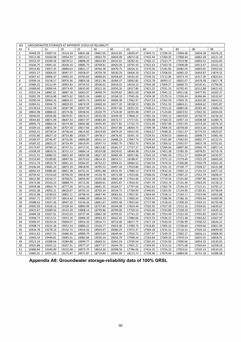
95

Appendix A8: Groundwater storage-reliability data of 100% GRSL

WEEK

GROUNDWATER STORAGES AT DIFFERENT LEVELS OF RELIABILITY5 10 20 25 30 40 50 60 70 80 90 98

1 19449.59 19387.52 19114.24 18831.68 18467.05 18322.85 18026.97 17445.71 17190.23 17004.48 16834.38 16376.222 19512.00 19260.08 19054.33 18913.22 18832.70 18459.08 18072.56 17455.44 17260.35 17008.44 16863.28 16121.193 19555.97 19190.58 18078.52 18898.29 18810.83 18433.91 18292.42 17460.15 17223.77 17019.98 16893.51 16163.854 19106.75 19041.41 18206.10 18885.73 18768.81 18420.39 18745.43 17422.63 17163.76 17008.08 16913.47 16161.145 19533.82 19057.35 18880.63 18821.17 18766.38 18470.75 18226.31 17370.50 17181.85 16982.65 16843.65 15952.026 19501.27 19004.03 18997.57 18558.07 18759.78 18530.29 18404.20 17322.56 17208.03 16965.53 16493.87 15874.557 19267.41 18906.47 19065.03 18783.60 18698.64 18358.69 18332.43 17339.33 17112.96 16973.74 16317.20 15823.618 19399.16 19158.57 18976.36 18803.58 18521.96 18366.37 18062.85 17422.78 16993.57 16855.07 16478.38 15817.789 19386.25 19112.95 18963.83 18734.53 18506.62 18416.02 18418.13 17434.38 17009.57 16860.73 16530.41 15796.9610 19368.60 19090.64 18973.49 18635.00 18321.16 18350.26 18317.80 17421.55 17031.53 16792.45 16512.88 16621.6211 19331.54 18962.61 18887.16 18563.97 18490.74 18199.82 18051.09 17369.99 17042.13 16911.06 16477.95 16202.2712 19281.29 18916.88 18875.62 18625.26 18480.12 18166.10 17945.26 17459.30 17170.13 17026.43 16366.66 16532.6713 19290.34 18904.26 18804.22 18655.73 18499.43 18406.38 17962.97 17547.53 17262.59 17003.76 16202.06 16643.5114 19269.41 19046.72 18829.93 18674.59 18460.26 18377.20 18158.51 17381.26 17251.50 16863.21 16404.62 15921.8715 19138.63 19161.08 18587.98 18567.99 18456.11 18367.06 18351.92 17506.21 17413.22 16882.06 16581.40 15686.3316 18843.98 18888.63 18574.06 18938.94 18320.79 17524.00 18393.48 17497.14 17124.84 16823.92 17042.36 16034.0317 19040.02 18926.86 18670.91 18624.25 18535.58 18349.30 17860.15 17301.34 17203.12 16819.82 16750.70 16236.2018 19043.83 18871.09 18647.54 18657.97 18483.20 18372.57 17717.01 17290.48 17160.33 16957.14 16508.38 16280.7519 18995.73 18864.54 18574.38 18692.86 18595.45 18277.82 17722.73 17222.40 17037.08 17037.03 16154.26 16376.1020 19209.16 18851.39 18707.18 18617.66 18576.13 18437.86 18064.73 17399.38 17068.33 16978.68 16553.26 16264.0821 19203.31 18728.54 18736.64 18614.83 18419.69 18479.29 18422.50 17464.57 17048.35 17021.47 16774.55 16620.0722 19192.80 18627.10 18733.88 18560.77 18478.17 18476.92 18391.10 17534.91 17039.53 16664.81 16898.73 16981.4023 19189.97 18746.47 18716.06 18600.89 18555.14 18488.23 17847.74 17509.43 17101.89 17042.93 16902.77 16122.4124 19183.32 18823.23 18729.49 18619.95 18597.73 18382.70 17852.75 17493.36 17200.52 17055.97 16815.78 16752.0125 19173.87 18789.13 18737.51 18717.41 18613.82 18181.57 17737.17 17494.84 17260.64 16897.69 16966.74 16857.1426 19108.59 18850.55 18731.23 18684.14 18533.08 18339.02 18049.38 17512.04 17452.38 17285.26 16978.01 16719.7627 19131.51 18980.22 18831.49 18693.98 18627.20 18485.49 18057.86 17543.10 17492.50 17311.27 16994.09 16535.9728 19153.60 19169.85 18847.56 18573.63 18614.25 18655.51 18188.47 17359.75 17372.13 17279.40 17025.29 16605.6029 19151.74 18919.74 18841.22 18564.47 18732.22 18964.22 18460.52 17160.54 17474.32 17206.88 17050.79 16561.2630 19106.04 19045.24 18872.29 18818.95 18795.52 18497.44 17910.86 17465.16 17331.31 17109.77 17028.27 16531.8831 18942.43 19086.60 18851.38 18731.41 18951.88 18531.95 17880.13 17474.93 17632.32 17065.12 17154.32 16677.2232 18739.42 19154.60 18799.59 18658.99 19139.76 18572.08 17923.66 17568.56 17768.35 17067.22 17053.79 16696.4733 18612.80 19234.27 18768.01 18656.00 19335.48 18602.48 17933.44 17532.39 17719.54 17101.80 17097.96 16653.3634 19473.06 19103.23 18888.74 18713.36 18669.61 18301.87 17834.45 17497.70 17353.76 17131.49 17063.35 16728.1335 19458.08 19063.74 18777.26 18711.26 18681.35 18164.57 17797.66 17461.63 17302.76 17146.33 17123.11 16792.1736 19502.38 19092.21 18620.07 18702.33 18703.54 18334.72 17789.94 17440.65 17265.92 17134.90 17185.81 16738.0437 19531.68 19249.62 18802.11 18796.43 18667.49 18063.62 17852.95 17604.40 17328.13 17160.17 17025.96 16455.8838 19567.71 19257.97 18814.42 19086.29 18836.54 17950.31 17860.34 17629.42 17286.99 17186.18 17003.64 16369.9039 19588.62 19247.26 18947.20 19136.26 18661.67 18391.48 17833.64 17777.99 17318.24 17209.29 17024.15 16720.4840 19492.93 19326.16 19104.34 18894.99 18737.85 18546.98 17824.44 17592.92 17327.39 17212.16 17034.02 16639.6741 19421.67 19289.56 19143.20 19008.14 18799.86 18700.08 17769.53 17420.46 17333.80 17228.39 17037.37 16635.1042 19484.18 19267.01 19142.03 18737.44 18862.28 18705.92 17741.23 17365.40 17353.40 17222.58 17055.82 16637.5443 19308.72 19215.51 19053.26 18984.39 18943.33 18562.45 17980.66 17423.55 17336.25 17222.48 17083.62 16567.9744 19309.47 19220.24 19069.07 18916.20 19016.71 18716.00 18017.72 17417.19 17343.54 17196.99 17036.52 16626.2245 19308.74 19225.36 19052.33 18886.22 19104.77 19019.46 17989.75 17418.85 17305.32 17238.64 17059.66 16821.9946 19426.78 19278.23 19192.72 19016.56 18929.97 18580.24 17972.37 17369.18 17231.52 17116.31 17026.32 16839.4047 19415.62 19437.91 19480.45 18989.79 18919.69 18649.44 17950.72 17297.97 17249.33 17062.17 16856.11 16808.9048 19403.54 19449.81 19685.01 18982.84 19030.24 18656.79 17948.34 17263.84 17309.26 17070.54 16655.01 16858.9149 19521.34 19388.64 19284.88 18999.77 18669.52 18342.04 17939.54 17365.45 17224.93 17090.66 16954.10 16530.0550 19501.88 19345.22 19257.91 18977.37 18677.57 18344.78 17901.21 17394.95 17213.52 17075.08 17049.64 16358.5951 19486.84 19340.00 19232.68 18973.75 18624.29 18398.56 17786.05 17416.35 17256.22 17053.61 17035.13 16534.3352 19485.91 19351.83 19175.87 18971.87 18710.89 18345.99 18115.72 17238.98 17070.09 16884.06 16731.18 16388.08