groundwater hydrology abdüsselam altunkaynak · groundwater hydrology abdüsselam altunkaynak page...

Groundwater Hydrology Abdüsselam ALTUNKAYNAK

Drawdown data Measurement

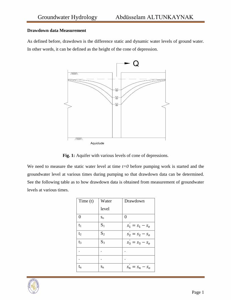
As defined before, drawdown is the difference static and dynamic water levels of ground water.

In other words, it can be defined as the height of the cone of depression.

Fig. 1: Aquifer with various levels of cone of depressions.

We need to measure the static water level at time t=0 before pumping work is started and the

groundwater level at various times during pumping so that drawdown data can be determined.

See the following table as to how drawdown data is obtained from measurement of groundwater

levels at various times.

Time (t) Water

level

Drawdown

0 so 0

t1 S1 𝑠1′ = 𝑠1 − 𝑠𝑜

t2 S2 𝑠2′ = 𝑠2 − 𝑠𝑜

t3 S3 𝑠3′ = 𝑠3 − 𝑠𝑜

. . .

. . .

tn sn 𝑠𝑛′ = 𝑠𝑛 − 𝑠𝑜


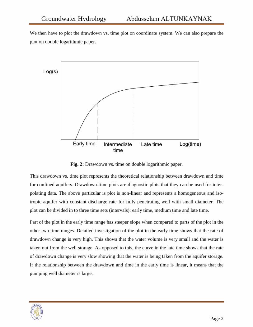
We then have to plot the drawdown vs. time plot on coordinate system. We can also prepare the

plot on double logarithmic paper.

Fig. 2: Drawdown vs. time on double logarithmic paper.

This drawdown vs. time plot represents the theoretical relationship between drawdown and time

for confined aquifers. Drawdown-time plots are diagnostic plots that they can be used for inter-

polating data. The above particular is plot is non-linear and represents a homogeneous and iso-

tropic aquifer with constant discharge rate for fully penetrating well with small diameter. The

plot can be divided in to three time sets (intervals): early time, medium time and late time.

Part of the plot in the early time range has steeper slope when compared to parts of the plot in the

other two time ranges. Detailed investigation of the plot in the early time shows that the rate of

drawdown change is very high. This shows that the water volume is very small and the water is

taken out from the well storage. As opposed to this, the curve in the late time shows that the rate

of drawdown change is very slow showing that the water is being taken from the aquifer storage.

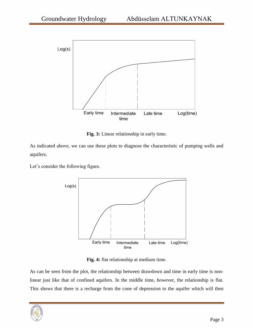
If the relationship between the drawdown and time in the early time is linear, it means that the

pumping well diameter is large.


Fig. 3: Linear relationship in early time.

As indicated above, we can use these plots to diagnose the characteristic of pumping wells and

aquifers.

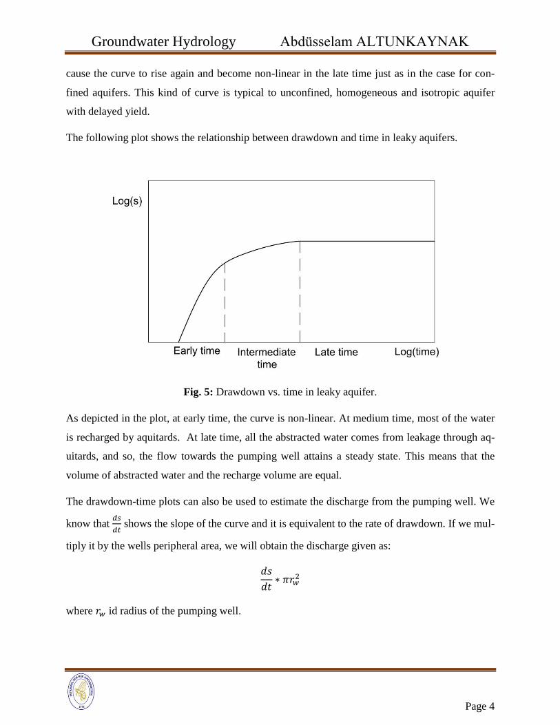
Let’s consider the following figure.

Fig. 4: flat relationship at medium time.

As can be seen from the plot, the relationship between drawdown and time in early time is non-

linear just like that of confined aquifers. In the middle time, however, the relationship is flat.

This shows that there is a recharge from the cone of depression to the aquifer which will then


cause the curve to rise again and become non-linear in the late time just as in the case for con-

fined aquifers. This kind of curve is typical to unconfined, homogeneous and isotropic aquifer

with delayed yield.

The following plot shows the relationship between drawdown and time in leaky aquifers.

Fig. 5: Drawdown vs. time in leaky aquifer.

As depicted in the plot, at early time, the curve is non-linear. At medium time, most of the water

is recharged by aquitards. At late time, all the abstracted water comes from leakage through aq-

uitards, and so, the flow towards the pumping well attains a steady state. This means that the

volume of abstracted water and the recharge volume are equal.

The drawdown-time plots can also be used to estimate the discharge from the pumping well. We

know that 𝑑𝑠

𝑑𝑡 shows the slope of the curve and it is equivalent to the rate of drawdown. If we mul-

tiply it by the wells peripheral area, we will obtain the discharge given as:

𝑑𝑠

𝑑𝑡∗ 𝜋𝑟𝑤

2

where 𝑟𝑤 id radius of the pumping well.


Partially penetrating wells

Theoretically, we assume the pumping well to be penetrating the aquifer fully. This forces the

flow towards the pumping well to have only horizontal component. Flow around the pumping

well will not only have horizontal component, but also a vertical component if the pumping well

is partially penetrating. The vertical component of flow results in extra head loss around the well.

Well-bore storage

In practice, we know that the volume of the well storage is very small when compared to the

aquifer storage. Because of this, the well storage is considered as line storage theoretically. As a

result, the effect of the well storage can be neglected.

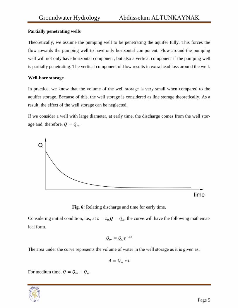
If we consider a well with large diameter, at early time, the discharge comes from the well stor-

age and, therefore, 𝑄 = 𝑄𝑤.

Fig. 6: Relating discharge and time for early time.

Considering initial condition, i.e., at 𝑡 = 𝑡𝑜,𝑄 = 𝑄𝑜, the curve will have the following mathemat-

ical form.

𝑄𝑤 = 𝑄𝑜𝑒−𝑎𝑡

The area under the curve represents the volume of water in the well storage as it is given as:

𝐴 = 𝑄𝑤 ∗ 𝑡

For medium time, 𝑄 = 𝑄𝑤 + 𝑄𝑤


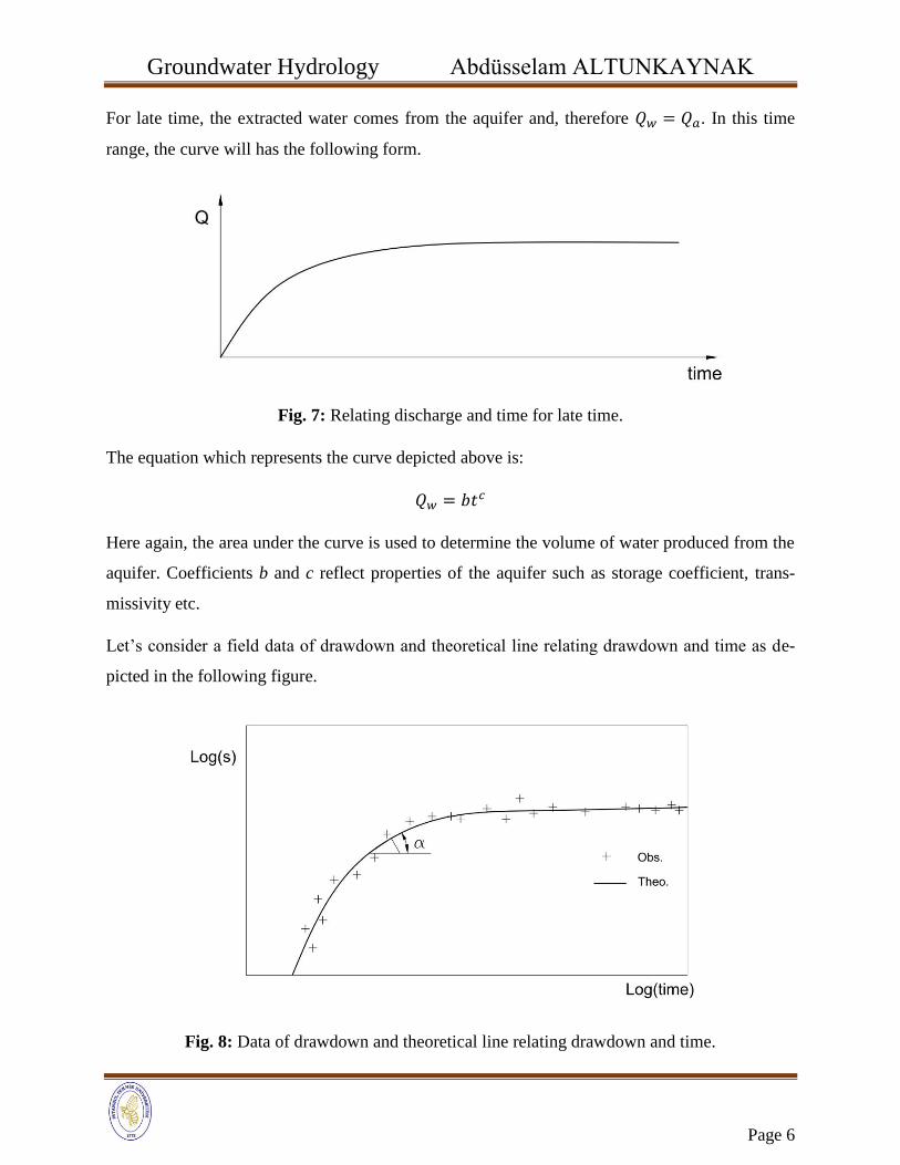
For late time, the extracted water comes from the aquifer and, therefore 𝑄𝑤 = 𝑄𝑎. In this time

range, the curve will has the following form.

Fig. 7: Relating discharge and time for late time.

The equation which represents the curve depicted above is:

𝑄𝑤 = 𝑏𝑡𝑐

Here again, the area under the curve is used to determine the volume of water produced from the

aquifer. Coefficients b and c reflect properties of the aquifer such as storage coefficient, trans-

missivity etc.

Let’s consider a field data of drawdown and theoretical line relating drawdown and time as de-

picted in the following figure.

Fig. 8: Data of drawdown and theoretical line relating drawdown and time.


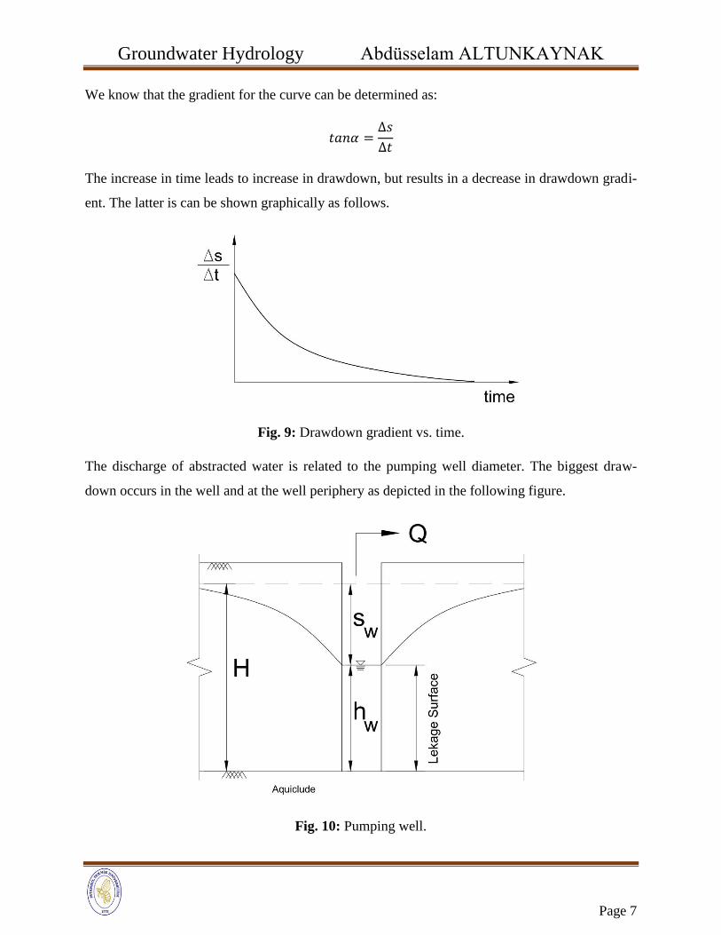
We know that the gradient for the curve can be determined as:

𝑡𝑎𝑛𝛼 =∆𝑠

∆𝑡

The increase in time leads to increase in drawdown, but results in a decrease in drawdown gradi-

ent. The latter is can be shown graphically as follows.

Fig. 9: Drawdown gradient vs. time.

The discharge of abstracted water is related to the pumping well diameter. The biggest draw-

down occurs in the well and at the well periphery as depicted in the following figure.

Fig. 10: Pumping well.


Let 𝑝𝑤 stand for perimeter of the pumping well and K stand for hydraulic conductivity. The

drawdown is a function of these variables.

∆𝑠 = 𝑓(𝑝𝑤,𝐾)

We know that ∆𝑠 ∝1

𝑝𝑤 and ∆𝑠 ∝

1

𝐾

This proportionality could be converted to the following two equalities.

∆𝑠 =𝐶

𝐾.𝑝𝑤 or ∆𝑠 =

𝑐1

𝐾+

𝑐2

𝑃𝑤

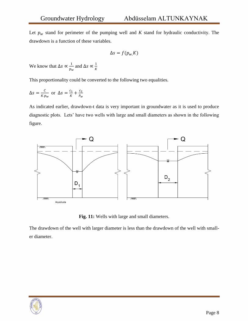
As indicated earlier, drawdown-t data is very important in groundwater as it is used to produce

diagnostic plots. Lets’ have two wells with large and small diameters as shown in the following

figure.

Fig. 11: Wells with large and small diameters.

The drawdown of the well with larger diameter is less than the drawdown of the well with small-

er diameter.


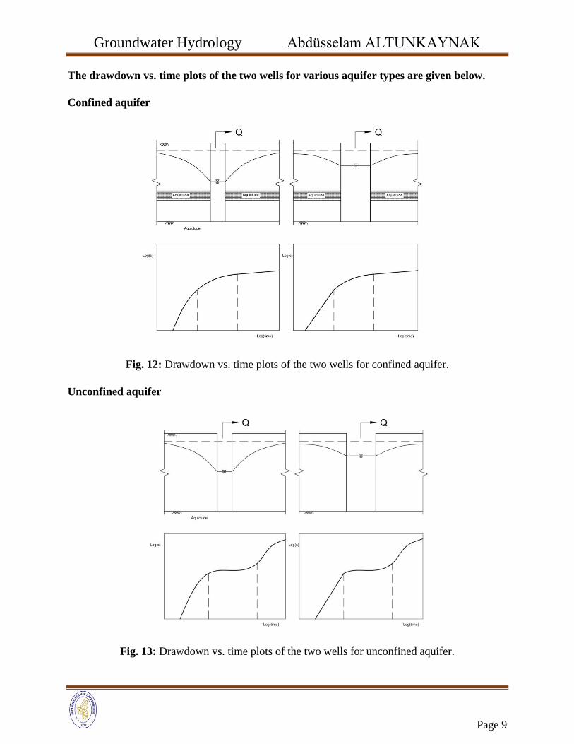
The drawdown vs. time plots of the two wells for various aquifer types are given below.

Confined aquifer

Fig. 12: Drawdown vs. time plots of the two wells for confined aquifer.

Unconfined aquifer

Fig. 13: Drawdown vs. time plots of the two wells for unconfined aquifer.


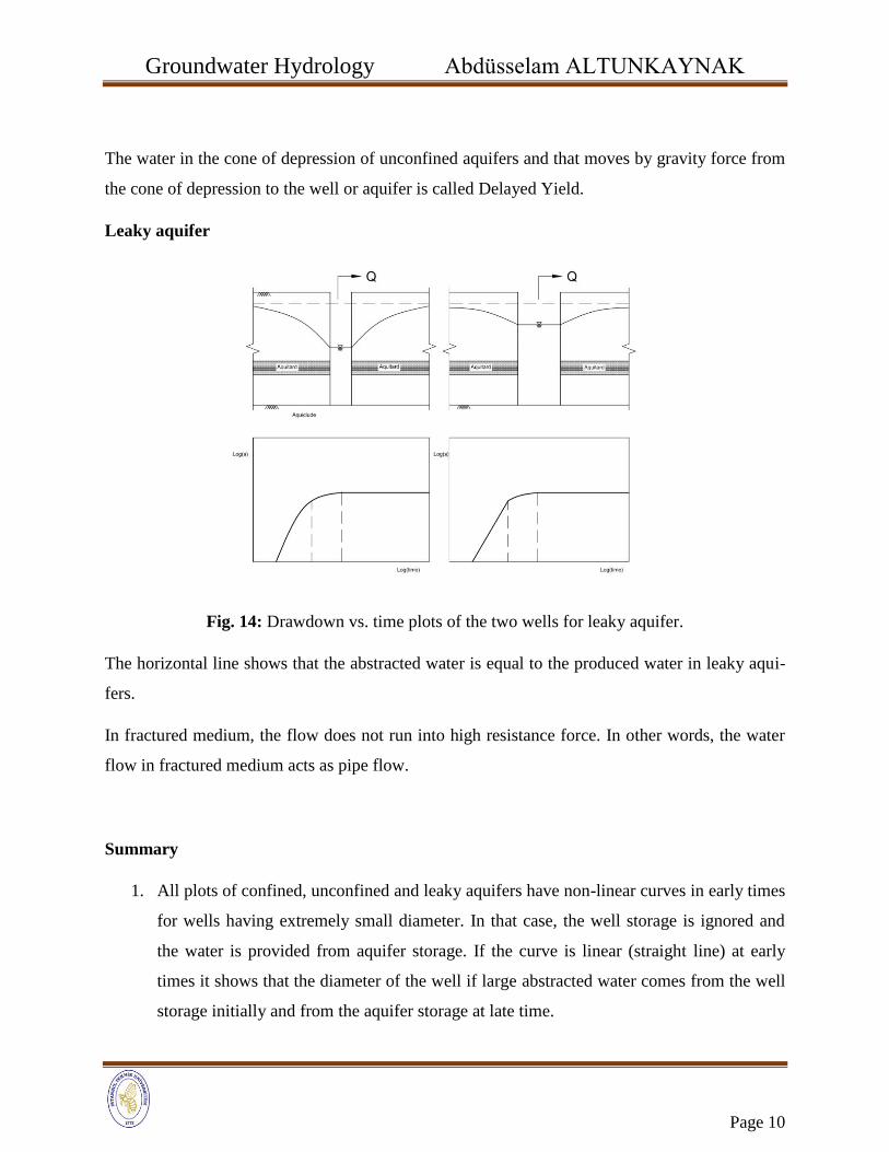
The water in the cone of depression of unconfined aquifers and that moves by gravity force from

the cone of depression to the well or aquifer is called Delayed Yield.

Leaky aquifer

Fig. 14: Drawdown vs. time plots of the two wells for leaky aquifer.

The horizontal line shows that the abstracted water is equal to the produced water in leaky aqui-

fers.

In fractured medium, the flow does not run into high resistance force. In other words, the water

flow in fractured medium acts as pipe flow.

Summary

1. All plots of confined, unconfined and leaky aquifers have non-linear curves in early times

for wells having extremely small diameter. In that case, the well storage is ignored and

the water is provided from aquifer storage. If the curve is linear (straight line) at early

times it shows that the diameter of the well if large abstracted water comes from the well

storage initially and from the aquifer storage at late time.


2. The drawdown tends to increase at late times in confined aquifers.

3. If there is a flat segment in the drawdown-t curve in medium times, it shows that the aq-

uifer is unconfined and there a delayed yield from the cone of depression to the aquifer

due to force of gravity.

4. If there is no change in drawdown at large times, this means that the aquifer is leaky aqui-

fer. In other words, at late times, a horizontal segment appears on the plot and it indicates

that steady state is reached.

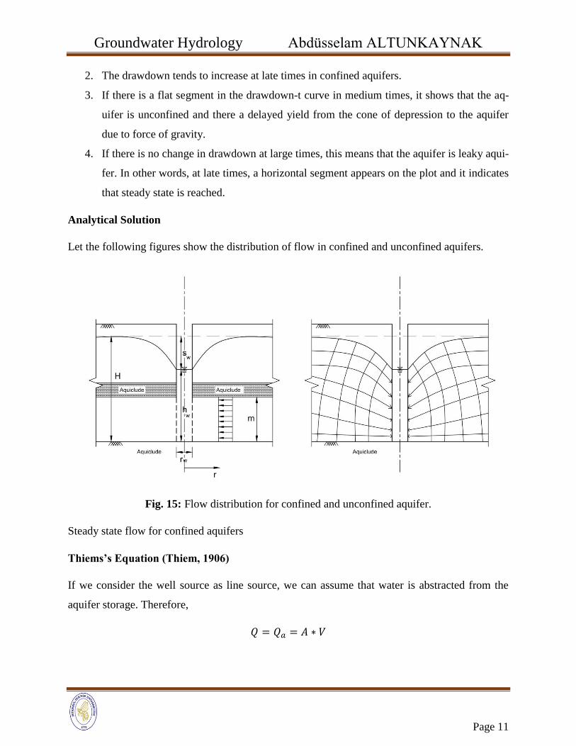
Analytical Solution

Let the following figures show the distribution of flow in confined and unconfined aquifers.

Fig. 15: Flow distribution for confined and unconfined aquifer.

Steady state flow for confined aquifers

Thiems’s Equation (Thiem, 1906)

If we consider the well source as line source, we can assume that water is abstracted from the

aquifer storage. Therefore,

𝑄 = 𝑄𝑎 = 𝐴 ∗ 𝑉


,where A is the area of the pumping well periphery give as 𝐴 = 2𝜋𝑟𝑚 and V is the velovity of

groundwater flow given by Darcy’s law as 𝑉 = 𝐾𝑑ℎ

𝑑𝑟

Therefore,

𝑄 = 2𝜋𝑟𝑚 ∗ 𝐾𝑑ℎ

𝑑𝑟

We know that 𝐾𝑚 = 𝑇. We also know that r is variable, whereas, m and K are constants.

This implies that

𝑄 = 2𝜋𝑟𝑇𝑑ℎ

𝑑𝑟 and

𝑄

2𝜋𝑇= ∫

𝑑ℎ

𝑟

𝐻𝑜

𝑟𝑤= ∫ 𝑑ℎ

𝑅

ℎ𝑤 considering boundary and initial conditions.

If we equate the above equation, we will get:

𝑄

2𝜋𝑇ln 𝑟/𝑟𝑤

𝑅 = ℎ/ℎ𝑤

𝐻𝑜

This implies that

𝑄

2𝜋𝑇(ln 𝑅 − 𝑙𝑛𝑟𝑤) = 𝐻𝑜 − ℎ𝑤

This implies that

𝑄

2𝜋𝑇ln (

𝑅

𝑟𝑤) = 𝐻𝑜 − ℎ𝑤

We know that 𝐻𝑜 − ℎ𝑤 = 𝑆𝑤. Therefore,

𝑇 =𝑄

2𝜋(𝐻𝑜 − ℎ𝑤)ln (

𝑅

𝑟𝑤)

We also know that ln (𝑅

𝑟𝑤) = 2.3 log (

𝑅

𝑟𝑤). Therefore,

𝑇 =2.3 𝑄

2𝜋(𝐻𝑜 − ℎ𝑤)log (

𝑅

𝑟𝑤)

,where, Q is discharge rate, H is static water level, hw is depth of water in the well, R is radius of

influence and rw is radius of the pumping well.


This is what is called Thiem’s equation and it can be used to determine transmissivity. This

equation does not tell anything about storage coefficient, though.

Let’s say that we collected drawdown data from the field at various radial distances from the

pumping well.

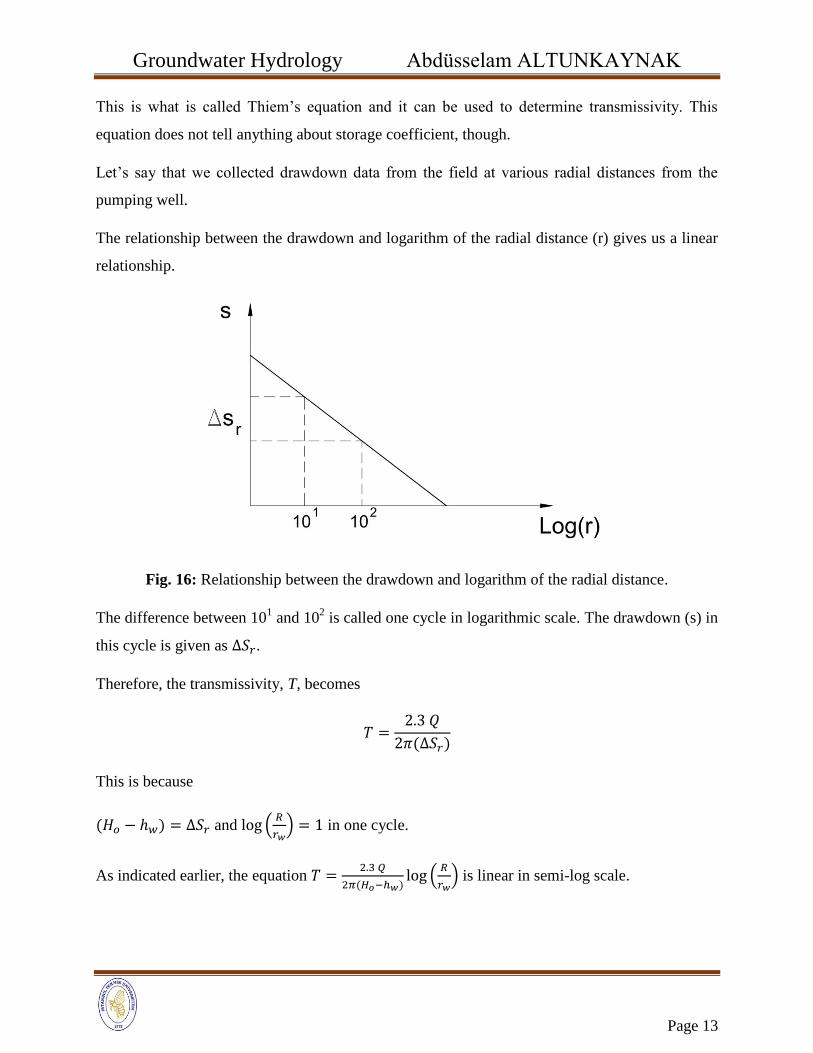
The relationship between the drawdown and logarithm of the radial distance (r) gives us a linear

relationship.

Fig. 16: Relationship between the drawdown and logarithm of the radial distance.

The difference between 101 and 10

2 is called one cycle in logarithmic scale. The drawdown (s) in

this cycle is given as ∆𝑆𝑟.

Therefore, the transmissivity, T, becomes

𝑇 =2.3 𝑄

2𝜋(∆𝑆𝑟)

This is because

(𝐻𝑜 − ℎ𝑤) = ∆𝑆𝑟 and log (𝑅

𝑟𝑤) = 1 in one cycle.

As indicated earlier, the equation 𝑇 =2.3 𝑄

2𝜋(𝐻𝑜−ℎ𝑤)log (

𝑅

𝑟𝑤) is linear in semi-log scale.


It is required to collect S data at least from three points. Then, we should plot S vs. distance on

semi-log paper. At the intercept of the linear line on the x-axis, s=0 and r=R. Therefore, we can

determine the value of radius of influence, R, by taking this point in to consideration.

R can also be determined from Thiem’s equation if we know the value of T. This means,

2𝜋𝑇(𝐻𝑜−ℎ𝑤)

2.3 𝑄= log (

𝑅

𝑟𝑤)or


𝑄= ln (

𝑅

𝑟𝑤)

This implies,

𝑅

𝑟𝑤= 𝑒


𝑄

Therefore,

𝑅 = 𝑟𝑤𝑒2𝜋𝑇(𝐻𝑜−ℎ𝑤)

𝑄

Unconfined Aquifer

The analytical solution of groundwater flow in unconfined aquifers is more complicated than confined

aquifers. This is because the thickness of the saturated zone decreases as we move closer towards the

well. In addition, flow lines are not parallel to each other in unconfined aquifers. Moreover, the ground-

water is recharged by infiltration in unconfined aquifers and they do not have regular geometry that the

analytical solution becomes more complicated.

As can be seen from the Figure 17, the gradient of the hydraulic head is steeper near the vicinity of the

pumping well showing that the drawdown is deeper around the well. Dupuit-Forcheimer derived analyti-

cal solution for steady state condition in unconfined aquifers by taking some assumptions into considera-

tion.

It is known that, for a saturated zone with thickness, h, the aquifer’s discharge (Q) at a radial distance (r)

can be written as follows from the continuity equation.


Fig. 17: unconfined aquifer and flow lines.

𝑄 = 2𝜋𝑟ℎ(𝑟)𝑞(𝑟)

or

𝑄 = 2𝜋𝑟ℎ(𝑟)𝐾𝑑ℎ

𝑑𝑟

Here, it should be noted that ℎ ∗ 𝐾 ≠ 𝑇 as the thickness, h, is not constant in unconfined aquifers.

If we divide Q by constant parameters and after some rearrangement, we will find:

𝑄

2𝜋𝐾

𝑑𝑟

𝑟= ℎ𝑑ℎ

Integration of both sides of the equation yields:

𝑄

2𝜋𝐾∫

𝑑𝑟

𝑟

𝑅

𝑟𝑤

= ∫ ℎ𝑑ℎ

𝐻𝑜

ℎ𝑤

⟹𝑄

2𝜋𝐾[𝑙𝑛𝑟]/𝑟𝑤

𝑅 =ℎ2

2/ℎ𝑤

𝐻𝑜 + 𝐶

After some mathematical manipulation and solving for K, we will find:

𝐾 =𝑄

𝜋.

ln (𝑅

𝑟𝑤)

(𝐻𝑜2 − 𝑟𝑤

2)


This equation can also be written as:

𝐾 =2.3𝑄

𝜋.

log (𝑅

𝑟𝑤)


2)

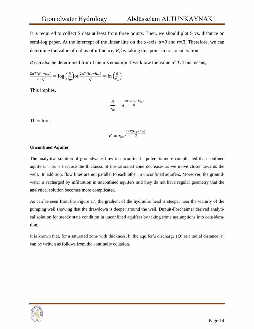
This equation is called Dupuit-Forcheimer equation. This equation can be used to calculate the hydraulic

conductivity for unconfined aquifers. In addition, the difference of the square of the hydraulic heads or

corresponding drawdown values vs. the radial distance can be plotted on a semi-log paper. This relation-

ship is linear on a semi-log paper as 2.3𝑄

𝜋(𝐻𝑜2−𝑟𝑤

2 ) is constant and log (

𝑅

𝑟𝑤) is a function.

Fig. 18: drawdown values vs. the radial distance.

For one cycle, on the semi-log paper, log (𝑅

𝑟𝑤) = 1.

Therefore, 𝐾 =2.3𝑄

𝜋.

log (𝑅

𝑟𝑤)

(𝐻𝑜2−𝑟𝑤

2 )= 𝐾 =

2.3𝑄

𝜋.

1

∆𝑆𝑟

Here, ∆𝑆𝑟 = (𝐻𝑜2 − 𝑟𝑤

2) and it is the slope of the graph.

In general, the Dupuit-Forcheimer equation exhibits a linear line between logarithmic radial distance and


2) values. This graphical method is valid for homogeneous and isotropic unconfined aquifer.


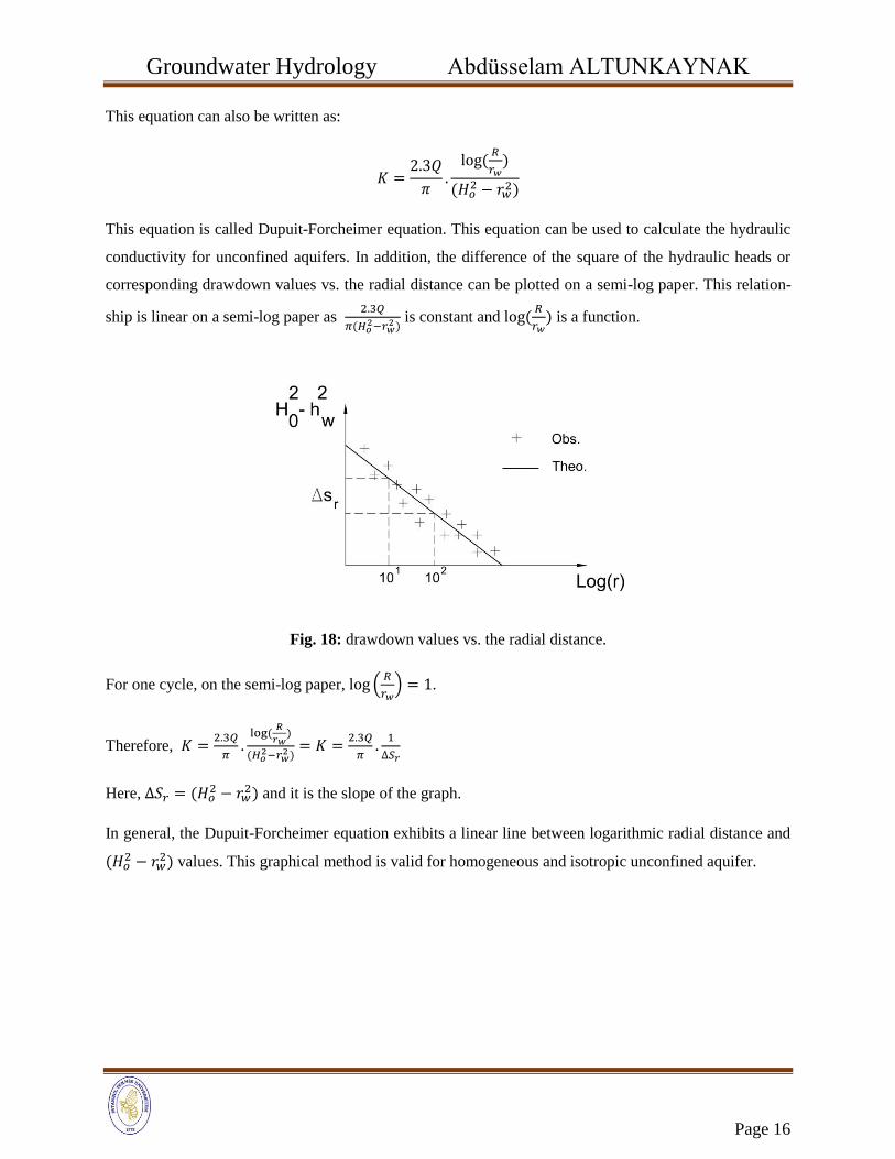
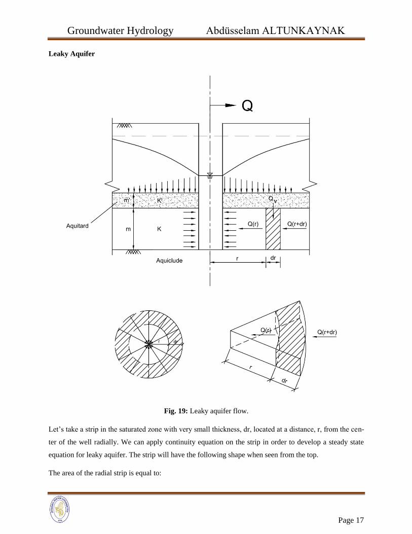
Leaky Aquifer

Fig. 19: Leaky aquifer flow.

Let’s take a strip in the saturated zone with very small thickness, dr, located at a distance, r, from the cen-

ter of the well radially. We can apply continuity equation on the strip in order to develop a steady state

equation for leaky aquifer. The strip will have the following shape when seen from the top.

The area of the radial strip is equal to:


𝐴 = (𝑟 + 𝑑𝑟)2𝜋 − 𝑟2𝜋 = 2𝜋𝑟𝑑𝑟 after ignoring (𝑑𝑟)2𝜋 for it is very small value.

Considering the inflows into the strip and outflow from the strip, we will get:

𝑄(𝑟 + 𝑑𝑟) − 𝑄(𝑟) + 𝑄𝑣 = 0

⟹ ∆𝑄(𝑟 + 𝑑𝑟) + 𝑄𝑣 = 0

This equation can be written in a differential form as:

𝜕𝑄(𝑟) + 2𝜋𝑟𝑑𝑟𝑞𝑣 = 0

𝑞𝑣 =𝐾′𝑆

𝑚′ for leaky aquifer.

Therefore,

𝜕𝑄(𝑟) + 2𝜋𝑟𝑑𝑟𝐾 ′𝑠

𝑚′= 0

If we divide both sides by 𝜕𝑟, we will get:

𝜕𝑄(𝑟)

𝜕𝑟+ 2𝜋𝑟

𝐾 ′𝑠

𝑚′= 0

We also know that discharge from aquifer (Q) can be written as:

𝑄 = −2𝜋𝑟𝑚𝐾𝑑𝑠

𝑑𝑟= 2𝜋𝑟𝑚𝐾

𝑑ℎ

𝑑𝑟

We know that 𝑚𝐾 = 𝑇

Therefore,

𝑄 = −2𝜋𝑇𝑟𝑑𝑠

𝑑𝑟

If we derivate both sides of the equation with respect to 𝑟, we will find”

𝜕𝑄

𝜕𝑟= −2𝜋𝑇(

𝑑𝑠

𝑑𝑟+ 𝑟

𝜕2𝑠

𝜕𝑟2)

If we substitute this equation into 𝜕𝑄(𝑟)

𝜕𝑟+ 2𝜋𝑟

𝐾′𝑠

𝑚′= 0, we will find:

−2𝜋𝑇 (𝑑𝑠

𝑑𝑟+ 𝑟

𝜕2𝑠

𝜕𝑟2) + 2𝜋𝑟𝐾 ′𝑠

𝑚′= 0


After canceling out 𝜋 and dividing the equation by T and r, we will get:

(𝑑𝑠

𝑟𝑑𝑟+

𝜕2𝑠

𝜕𝑟2) −𝐾 ′𝑠

𝑇𝑚′= 0

From our earlier definitions, we know that Hydraulic resistance (HR) and Leakage factor (L) are giv-

en as:

𝐻𝑅 =𝑚′

𝐾′ and 𝐿 = √𝑇𝐻𝑅.

This implies that 𝐿2 = 𝑇𝐻𝑅 and 1

𝐿2 =1

𝑇𝐻𝑅. Therefore,

1

𝐿2 =1

𝑇

𝐾′

𝑚′

Substituting these relationships in the above equation, we will get:

(𝜕2𝑠

𝜕𝑟2+

𝑑𝑠

𝑟𝑑𝑟) −

𝑠(𝑟)

𝐿2= 0

This equation needs to be solved and the solution becomes:

𝑠(𝑟) = 𝐶1𝐼𝑜 (𝑟

𝐿) + 𝐶2𝐾𝑜 (

𝑟

𝐿)

Here, 𝐶1 and 𝐶2 are constants.

𝐼𝑜 (𝑟

𝐿) is a zero-order modified function and 𝐾𝑜 (

𝑟

𝐿) is a zero-order modified function called Bessel func-

tion.

Taking boundary conditions into consideration, for infinite aquifer, the boundary condition at infinity is:

When 𝑟 → ∞, 𝑠(𝑟) = 0 and ℎ = 𝐻 . In this case, 𝐼𝑜 (𝑟

𝐿) = (∞) = ∞ and 𝐾𝑜 (

𝑟

𝐿) = 𝐾𝑜(∞) = 0

Therefore,

𝑠(∞) = 𝐶1𝐼𝑜(∞) + 𝐶2𝐾𝑜(∞)

This implies that:

0 = 𝐶1𝐼𝑜(∞) + 𝐶2(0)

Solving for 𝐶1, we will get:𝐶1 = 0.

Taking initial condition in to consideration, i.e., 𝑟 = 𝑟𝑤,


and 𝐶2𝐾𝑜 (𝑟

𝐿) = 0. This implies that:

𝐶1 = 0

When 𝑟 = 𝑟𝑤,

𝑄 = −2𝜋𝑟𝑤𝑚𝐾𝑑𝑠

𝑑𝑟

This implies:

𝑄 = −2𝜋𝑟𝑤𝑚𝐾𝐶2

1

𝐿𝐾1 (

𝑟𝑤

𝐿)

Therefore,

𝐶2 = −𝑄

2𝜋𝑇 (𝑟𝑤

𝐿) 𝐾1 (

𝑟𝑤

𝐿)

After substituting 𝐶1 and 𝐶2 into the main equation, we will find:

𝑠(𝑟) = 𝐶1𝐼𝑜 (𝑟

𝐿) + 𝐶2𝐾𝑜 (

𝑟

𝐿)

𝑠(𝑟) =𝑄

2𝜋𝑇

𝐾𝑜 (𝑟

𝐿)

(𝑟𝑤

𝐿) 𝐾1 (

𝑟𝑤

𝐿)

By definition,

(𝑟𝑤

𝐿) = 𝑟𝑤

√𝐾 ′

𝑚𝑚′𝐾

In practice (Marino and Luthin, 1982)

For 𝑟𝑤

𝐿< 0.01, (

𝑟𝑤

𝐿) 𝐾1 (

𝑟𝑤

𝐿) ≅ 1

Taking this into consideration, the final form of the equation for steady state flow in leaky aquifers will

become:

𝑠(𝑟) ≅𝑄

2𝜋𝑇 𝐾𝑜 (

𝑟

𝐿)


This is called De Glee Equation (De Glee, 1930). This equation was cited by Kruseman and De Ridder

(1994). The same equation was proposed by Hantush and Jacob (1955) without realizing the work done

by De Glee undertaken 25 year earlier. Hantush (1964) indicated that:

If 𝑟

𝐿 is small (

𝑟

𝐿≤ 0.05) the equation can be taken to find approximate values as:

𝑠(𝑟) ≅2.30 𝑄

2𝜋𝑇𝑙𝑜𝑔 (

1.12𝐿

𝑟)

If we develop a plot relating 𝐾𝑜 (𝑟

𝐿) and (

𝑟

𝐿) on a log-log (double log) paper, we will find the following

type curve.

Fig. 20: Relationship between K0(r/L) and (r/L).

Unsteady State Flow

The main purpose of pumping test is in order to find hydraulic parameters by using measured drawdown-

time data in the pumping well and piezometers. In other words, we have to use measured field data and

theoretical models together in order to determine discharge rate, hydraulic conductivity, transmissivity

coefficient, storage coefficient, leakage factor and radius of influence of the well. The determination of

hydraulic and aquifer parameters is very important in terms of planning design operation and management

of groundwater resource.

Interpretation of aquifer parameters

The discharge rate, transmissivity, storage coefficient and leakage factor show aquifer properties. When

we compare aquifers, not all these parameters are considered as variables at a time. One parameter is


taken as a variable while the others are considers constants during pumping tests of groundwater. In other

words, among discharge rate, transmissivity coefficient, storage coefficient and leakage factor, one pa-

rameter is taken as variable and the remaining parameters are considered to be constants.

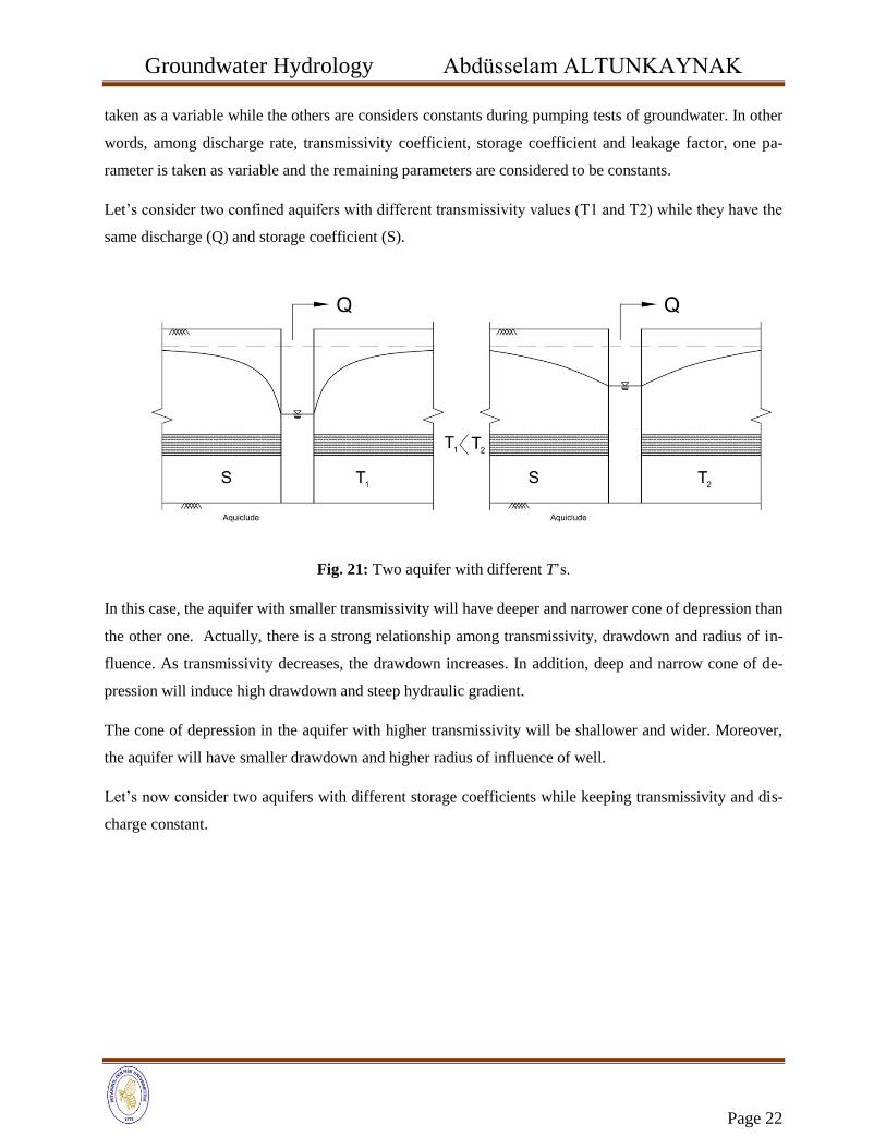
Let’s consider two confined aquifers with different transmissivity values (T1 and T2) while they have the

same discharge (Q) and storage coefficient (S).

Fig. 21: Two aquifer with different T’s.

In this case, the aquifer with smaller transmissivity will have deeper and narrower cone of depression than

the other one. Actually, there is a strong relationship among transmissivity, drawdown and radius of in-

fluence. As transmissivity decreases, the drawdown increases. In addition, deep and narrow cone of de-

pression will induce high drawdown and steep hydraulic gradient.

The cone of depression in the aquifer with higher transmissivity will be shallower and wider. Moreover,

the aquifer will have smaller drawdown and higher radius of influence of well.

Let’s now consider two aquifers with different storage coefficients while keeping transmissivity and dis-

charge constant.


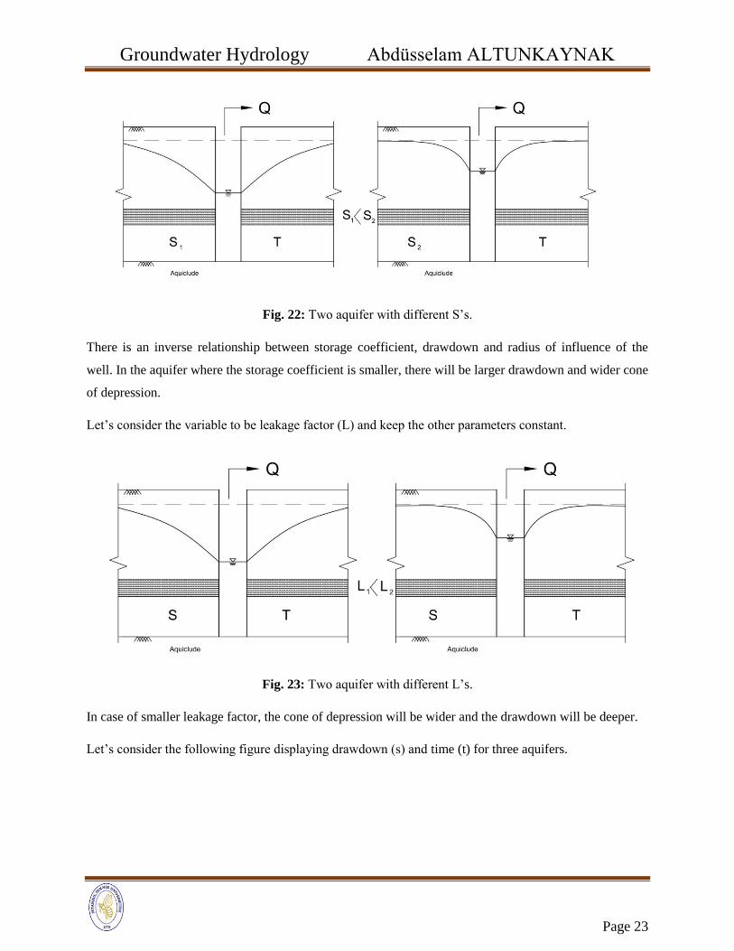
Fig. 22: Two aquifer with different S’s.

There is an inverse relationship between storage coefficient, drawdown and radius of influence of the

well. In the aquifer where the storage coefficient is smaller, there will be larger drawdown and wider cone

of depression.

Let’s consider the variable to be leakage factor (L) and keep the other parameters constant.

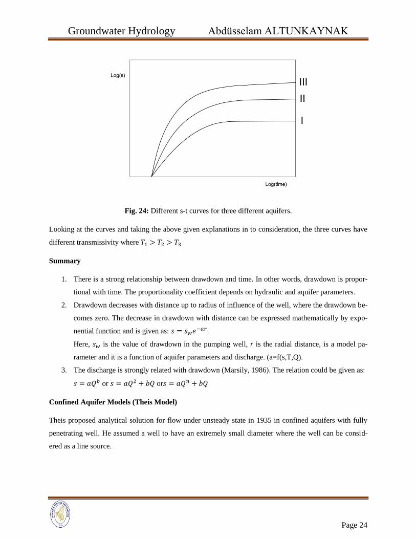
Fig. 23: Two aquifer with different L’s.

In case of smaller leakage factor, the cone of depression will be wider and the drawdown will be deeper.

Let’s consider the following figure displaying drawdown (s) and time (t) for three aquifers.


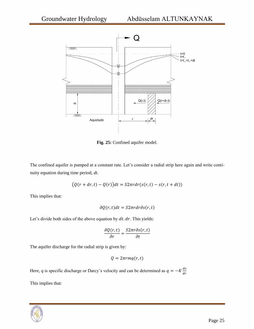
Fig. 24: Different s-t curves for three different aquifers.

Looking at the curves and taking the above given explanations in to consideration, the three curves have

different transmissivity where 𝑇1 > 𝑇2 > 𝑇3

Summary

1. There is a strong relationship between drawdown and time. In other words, drawdown is propor-

tional with time. The proportionality coefficient depends on hydraulic and aquifer parameters.

2. Drawdown decreases with distance up to radius of influence of the well, where the drawdown be-

comes zero. The decrease in drawdown with distance can be expressed mathematically by expo-

nential function and is given as: 𝑠 = 𝑠𝑤𝑒−𝑎𝑟.

Here, 𝑠𝑤 is the value of drawdown in the pumping well, r is the radial distance, is a model pa-

rameter and it is a function of aquifer parameters and discharge. (a=f(s,T,Q).

3. The discharge is strongly related with drawdown (Marsily, 1986). The relation could be given as:

𝑠 = 𝑎𝑄𝑏 or 𝑠 = 𝑎𝑄2 + 𝑏𝑄 or𝑠 = 𝑎𝑄𝑛 + 𝑏𝑄

Confined Aquifer Models (Theis Model)

Theis proposed analytical solution for flow under unsteady state in 1935 in confined aquifers with fully

penetrating well. He assumed a well to have an extremely small diameter where the well can be consid-

ered as a line source.


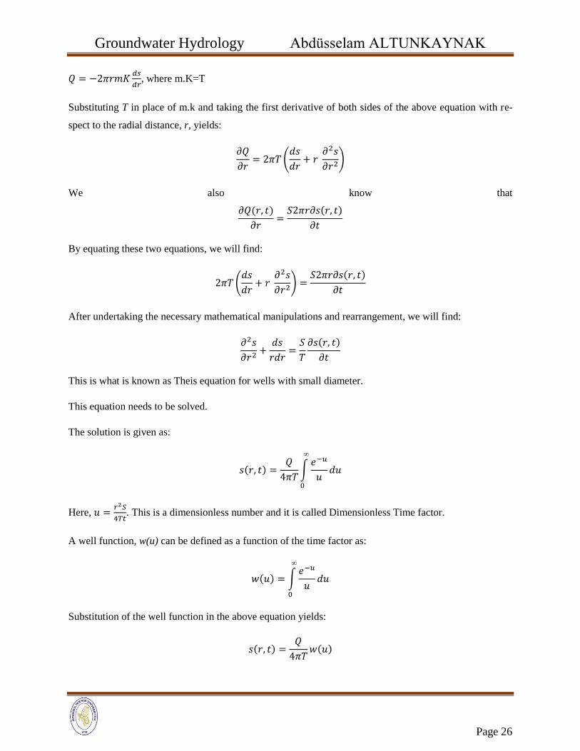
Fig. 25: Confined aquifer model.

The confined aquifer is pumped at a constant rate. Let’s consider a radial strip here again and write conti-

nuity equation during time period, dt.

(𝑄(𝑟 + 𝑑𝑟, 𝑡) − 𝑄(𝑟))𝑑𝑡 = 𝑆2𝜋𝑟𝑑𝑟(𝑠(𝑟, 𝑡) − 𝑠(𝑟, 𝑡 + 𝑑𝑡))

This implies that:

𝜕𝑄(𝑟, 𝑡)𝑑𝑡 = 𝑆2𝜋𝑟𝑑𝑟𝜕𝑠(𝑟, 𝑡)

Let’s divide both sides of the above equation by 𝑑𝑡. 𝑑𝑟. This yields:

𝜕𝑄(𝑟, 𝑡)

𝜕𝑟=

𝑆2𝜋𝑟𝜕𝑠(𝑟, 𝑡)

𝜕𝑡

The aquifer discharge for the radial strip is given by:

𝑄 = 2𝜋𝑟𝑚𝑞(𝑟, 𝑡)

Here, q is specific discharge or Darcy’s velocity and can be determined as 𝑞 = −𝐾𝑑𝑠

𝑑𝑟

This implies that:


𝑄 = −2𝜋𝑟𝑚𝐾𝑑𝑠

𝑑𝑟, where m.K=T

Substituting T in place of m.k and taking the first derivative of both sides of the above equation with re-

spect to the radial distance, r, yields:

𝜕𝑄

𝜕𝑟= 2𝜋𝑇 (

𝑑𝑠

𝑑𝑟+ 𝑟

𝜕2𝑠

𝜕𝑟2)

We also know that

𝜕𝑄(𝑟, 𝑡)

𝜕𝑟=

𝑆2𝜋𝑟𝜕𝑠(𝑟, 𝑡)

𝜕𝑡

By equating these two equations, we will find:

2𝜋𝑇 (𝑑𝑠

𝑑𝑟+ 𝑟

𝜕2𝑠

𝜕𝑟2) =𝑆2𝜋𝑟𝜕𝑠(𝑟, 𝑡)

𝜕𝑡

After undertaking the necessary mathematical manipulations and rearrangement, we will find:

𝜕2𝑠

𝜕𝑟2+

𝑑𝑠

𝑟𝑑𝑟=

𝑆

𝑇

𝜕𝑠(𝑟, 𝑡)

𝜕𝑡

This is what is known as Theis equation for wells with small diameter.

This equation needs to be solved.

The solution is given as:

𝑠(𝑟, 𝑡) =𝑄

4𝜋𝑇∫

𝑒−𝑢

𝑢

∞

0

𝑑𝑢

Here, 𝑢 =𝑟2𝑆

4𝑇𝑡. This is a dimensionless number and it is called Dimensionless Time factor.

A well function, w(u) can be defined as a function of the time factor as:

𝑤(𝑢) = ∫𝑒−𝑢

𝑢

∞

0

𝑑𝑢

Substitution of the well function in the above equation yields:


4𝜋𝑇𝑤(𝑢)


This implies:

𝑤(𝑢) =4𝜋𝑇

𝑄𝑠(𝑟)

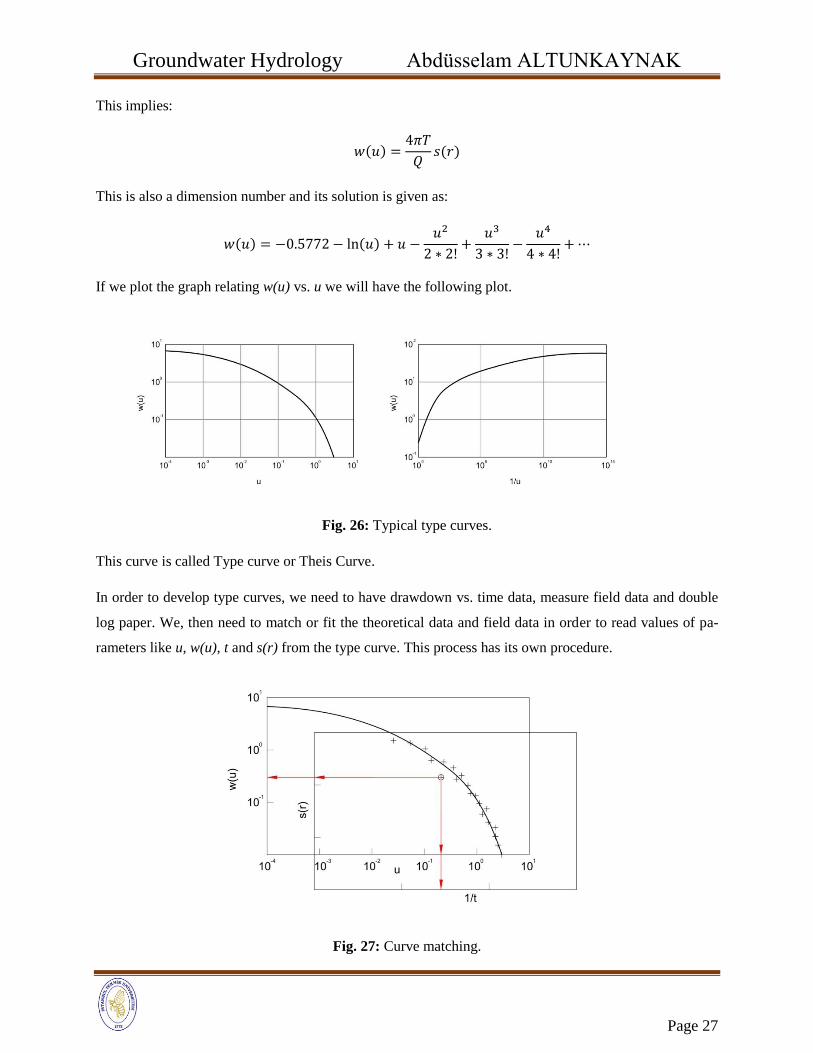
This is also a dimension number and its solution is given as:

𝑤(𝑢) = −0.5772 − ln(𝑢) + 𝑢 −𝑢2

2 ∗ 2!+

𝑢3

3 ∗ 3!−

𝑢4

4 ∗ 4!+ ⋯

If we plot the graph relating w(u) vs. u we will have the following plot.

Fig. 26: Typical type curves.

This curve is called Type curve or Theis Curve.

In order to develop type curves, we need to have drawdown vs. time data, measure field data and double

log paper. We, then need to match or fit the theoretical data and field data in order to read values of pa-

rameters like u, w(u), t and s(r) from the type curve. This process has its own procedure.

Fig. 27: Curve matching.


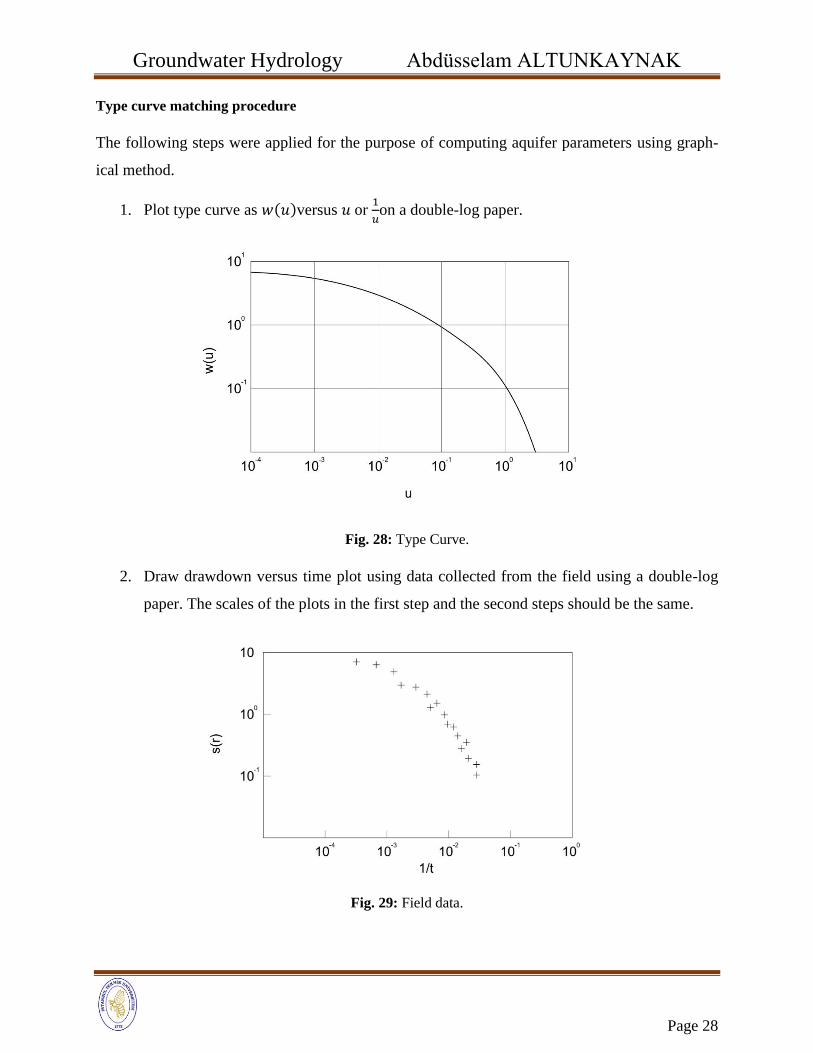
Type curve matching procedure

The following steps were applied for the purpose of computing aquifer parameters using graph-

ical method.

1. Plot type curve as 𝑤(𝑢)versus 𝑢 or 1

𝑢on a double-log paper.

Fig. 28: Type Curve.

2. Draw drawdown versus time plot using data collected from the field using a double-log

paper. The scales of the plots in the first step and the second steps should be the same.

Fig. 29: Field data.


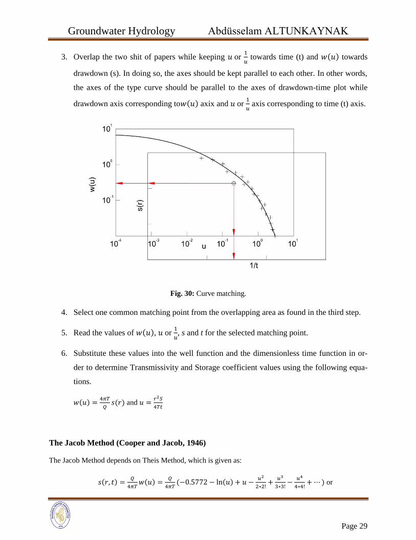
3. Overlap the two shit of papers while keeping 𝑢 or 1

𝑢 towards time (t) and 𝑤(𝑢) towards

drawdown (s). In doing so, the axes should be kept parallel to each other. In other words,

the axes of the type curve should be parallel to the axes of drawdown-time plot while

drawdown axis corresponding to𝑤(𝑢) axix and 𝑢 or 1

𝑢 axis corresponding to time (t) axis.

Fig. 30: Curve matching.

4. Select one common matching point from the overlapping area as found in the third step.

5. Read the values of 𝑤(𝑢), 𝑢 or 1

𝑢, s and t for the selected matching point.

6. Substitute these values into the well function and the dimensionless time function in or-

der to determine Transmissivity and Storage coefficient values using the following equa-

tions.

𝑤(𝑢) =4𝜋𝑇

𝑄𝑠(𝑟) and 𝑢 =

𝑟2𝑆

4𝑇𝑡

The Jacob Method (Cooper and Jacob, 1946)

The Jacob Method depends on Theis Method, which is given as:


4𝜋𝑇𝑤(𝑢) =

𝑄

4𝜋𝑇(−0.5772 − ln(𝑢) + 𝑢 −

𝑢2

2∗2!+

𝑢3

3∗3!−

𝑢4

4∗4!+ ⋯ ) or


𝑤(𝑢) = −0.5772 − ln(𝑢) + 𝑢 −𝑢2

2 ∗ 2!+

𝑢3

3 ∗ 3!−

𝑢4

4 ∗ 4!+ ⋯

The dimensionless time factor is given by 𝑢 =𝑟2𝑆

4𝑇𝑡.

Jacob noticed that there is an inverse relationship between time factor (u) and time (t). The time factor

increases as the pumping period increases. In addition the time factor decreases as radial distance from

the pumping well increases. After a certain large pumping period or large time, the value of u becomes

very small the u terms given in the well function become extremely small except that of (−0.5772 −

ln(𝑢)). Therefore, the terms beyond −0.5772 − ln(𝑢) can be neglected. This implies that:

𝑤(𝑢) = −0.5772 − ln(𝑢)

In this case, the drawdown can be approximated by:



𝑄

4𝜋𝑇(−0.5772 − ln(𝑢))

−0.5772can be expressed in terms of natural log as ln 𝐶 = − 0.5772 which makes 𝐶 = 0.5614

Therefore,



𝑄

4𝜋𝑇(−0.5772 − ln(𝑢)) =

𝑄

4𝜋𝑇(𝑙𝑛0.5614 − ln (

𝑟2𝑆

4𝑇𝑡))

This implies that


4𝜋𝑇(𝑙𝑛0.5614 + ln (

4𝑇𝑡

𝑟2𝑆))


4𝜋𝑇(ln (

0.5614 ∗ 4𝑇𝑡

𝑟2𝑆))

Therefore,


4𝜋𝑇(ln (

2.25𝑇𝑡

𝑟2𝑆))

When written in terms of common log, the equation becomes:

𝑠(𝑟, 𝑡) =2.3 𝑄

4𝜋𝑇(log (

2.25𝑇𝑡

𝑟2𝑆))

Here, Q, S and T are constants


The equation is linear as the 2.3 𝑄

4𝜋𝑇 component is constant and is taken as the slope of function log (

2.25𝑇𝑡

𝑟2𝑆).

If the drawdown versus time plot is drawn on a semi-log paper using the measured data, linear line can be

fit on the drawdown-time data. If this linear line is extended up to the time intercept, it will, i.e, up to the

point where the linear line meets the time axis, we can find the point where the drawdown (s) is equal to

zero. In other words, under this circumstance, s = 0 and 𝑡 = 𝑡𝑜.

If we take this point into consideration and substitute these values in the above given equation, we will

find:

0 =2.3 𝑄

4𝜋𝑇(log (

2.25𝑇𝑡𝑜

𝑟2𝑆))

This implies that

log (2.25𝑇𝑡𝑜

𝑟2𝑆) = 0

Therefore,

2.25𝑇𝑡𝑜

𝑟2𝑆= 1

Hence,

𝑆 =2.25𝑇𝑡𝑜

𝑟2

As indicated earlier, the 2.3 𝑄

4𝜋𝑇 component is constant and is taken as the slope of the linear function

log (2.25𝑇𝑡

𝑟2𝑆).

If we consider one log cycle of time, i.e., log (𝑡

𝑡𝑜) = 1, the slope of the linear line becomes the difference

between two successive drawdowns (∆𝑠).

This can be written as:

∆𝑠 =2.3 𝑄

4𝜋𝑇

This implies that:

𝑇 =2.3 𝑄

4𝜋∆𝑠


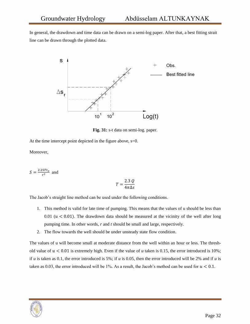
In general, the drawdown and time data can be drawn on a semi-log paper. After that, a best fitting strait

line can be drawn through the plotted data.

Fig. 31: s-t data on semi-log. paper.

At the time intercept point depicted in the figure above, s=0.

Moreover,

𝑆 =2.25𝑇𝑡𝑜

𝑟2 and

𝑇 =2.3 𝑄

4𝜋∆𝑠

The Jacob’s straight line method can be used under the following conditions.

1. This method is valid for late time of pumping. This means that the values of u should be less than

0.01 (𝑢 < 0.01). The drawdown data should be measured at the vicinity of the well after long

pumping time. In other words, r and t should be small and large, respectively.

2. The flow towards the well should be under unsteady state flow condition.

The values of u will become small at moderate distance from the well within an hour or less. The thresh-

old value of 𝑢 < 0.01 is extremely high. Even if the value of u taken is 0.15, the error introduced is 10%;

if u is taken as 0.1, the error introduced is 5%; if u is 0.05, then the error introduced will be 2% and if u is

taken as 0.03, the error introduced will be 1%. As a result, the Jacob’s method can be used for 𝑢 < 0.1.


The steps of Jacob’s method

1. Draw drawdown vs. time on a semi-log paper. This means that drawdown on linear scale and

time on logarithmic scale are plotted

2. Fit the best-fit straight line through the measured data plotted in step 1.

3. Extend the straight line up to the time intercept point, where s = 0 and𝑡 = 𝑡𝑜.

4. Determine the difference in drawdown (∆𝑠), which corresponds to the slope of straight line within

one log cycle.

5. Use the equations in order to determine parameters T and S using the following equations.

𝑆 = 2.25𝑇𝑡𝑜

𝑟𝑜2 and 𝑇 =

2.3 𝑄

4𝜋∆𝑠

6. After determining S and T, compute u from 𝑢 = (𝑟2𝑆

4𝑇𝑡) to verify whether is < 0.01 and check

practicability of Jacob’s method.

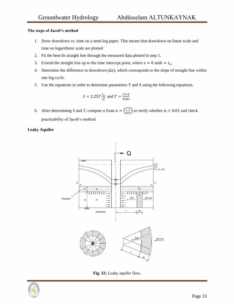
Leaky Aquifer

Fig. 32: Leaky aquifer flow.


In leaky aquifers under unsteady state flow condition, flow comes from every direction towards the circu-

lar strip and the continuity equation for the circular strip can be expressed as:

(𝑄(𝑟 + 𝑑𝑟, 𝑡) − 𝑄(𝑟))𝑑𝑡 + 𝑄𝑣𝑑𝑡 = −𝑆2𝜋𝑟𝑑𝑟(𝑠(𝑟, 𝑡) − 𝑠(𝑟, 𝑡 + 𝑑𝑡))

This implies that:

𝜕𝑄(𝑟, 𝑡)𝑑𝑡 + 𝑄𝑣𝑑𝑡 = −𝑆2𝜋𝑟𝑑𝑟𝜕𝑠(𝑟, 𝑡)

If we divide both sides of the above equation by ‘dt’ and ‘dr’, it becomes:

𝜕𝑄(𝑟, 𝑡)

𝜕𝑟+

𝜕𝑄𝑣

𝜕𝑟=

−𝑆2𝜋𝑟𝜕𝑠(𝑟, 𝑡)

𝜕𝑡

We know that

𝑄𝑣 = 2𝜋𝑟𝑑𝑟𝐾 ′𝑠

𝑚′

If we substitute this equation in the above equation, the result will be:

𝜕𝑄(𝑟, 𝑡)

𝜕𝑟+

2𝜋𝑟𝑑𝑟𝐾′𝑠

𝑚′

𝜕𝑟=


𝜕𝑡

Therefore,

𝜕𝑄(𝑟, 𝑡)

𝜕𝑟+ 2𝜋𝑟

𝐾 ′𝑠

𝑚′=


𝜕𝑡

From continuity equation, we have 𝑄 = −2𝜋𝑟𝑚𝐾𝜕𝑠

𝜕𝑟

If we substitute m.K by T and derivate both sides of this equation with respect to r, we will find”

𝜕𝑄

𝜕𝑟= −2𝜋𝑇 (

𝜕𝑠

𝜕𝑟+ 𝑟

𝜕2𝑠

𝜕𝑟2)

If we substitute this equation in the above given continuity equation, we will find:

−2𝜋𝑇 (𝜕𝑠

𝜕𝑟+ 𝑟

𝜕2𝑠

𝜕𝑟2) + 2𝜋𝑟𝐾 ′𝑠

𝑚′=


𝜕𝑡

Dividing both sides of this equation by −2𝜋𝑇 yields:


𝜕𝑠

𝜕𝑟+ 𝑟

𝜕2𝑠

𝜕𝑟2−

𝑟𝐾 ′𝑠

𝑇𝑚′=

−𝑆𝑟𝜕𝑠(𝑟, 𝑡)

𝑇𝜕𝑡

We also know that 𝐾′

𝑇𝑚′=

1

𝐿2, where L is leakage factor.

If we substitute this value in the above equation and divide both sides by r, we will obtain:

𝜕2𝑠

𝜕𝑟2+

1

𝑟

𝜕𝑠

𝜕𝑟−

𝑠

𝐿2=

𝑆

𝑇

𝜕𝑠(𝑟, 𝑡)

𝜕𝑡

This equation has three unknown parameters: T, L and S.

Hantush and Jacob in 1955 solved this equation and derived the equation for leaky aquifer under unsteady

state flow, which is given as:


4𝜋𝑇[∫

1

𝑦𝑒

−𝑦−𝑟2

4𝐿2𝑦. 𝑑𝑦

∞

𝑢

]

Here, a well function can be introduced as 𝑤 (𝑢,𝑟

𝐿) = ∫

1

𝑦𝑒

−𝑦−𝑟2

4𝐿2𝑦. 𝑑𝑦∞

𝑢

This implies:


4𝜋𝑇𝑤 (𝑢,

𝑟

𝐿)

𝑤 (𝑢,𝑟

𝐿) =

4𝜋𝑇

𝑄𝑠(𝑟, 𝑡)

𝑟

𝐿 is denoted by 𝛽 and, therefore,

𝑤(𝑢, 𝛽) = ∫1

𝑦𝑒

−𝑦−𝛽2

4𝑦 . 𝑑𝑦 =4𝜋𝑇

𝑄𝑠(𝑟, 𝑡)

∞

𝑢

This implies that

This function is known as Hantush and Jacob well function for leaky aquifer.

If we plot a type curve of 𝑤(𝑢, 𝛽) vs. u, we will have a plot as depicted in following figure for different

values of 𝛽.


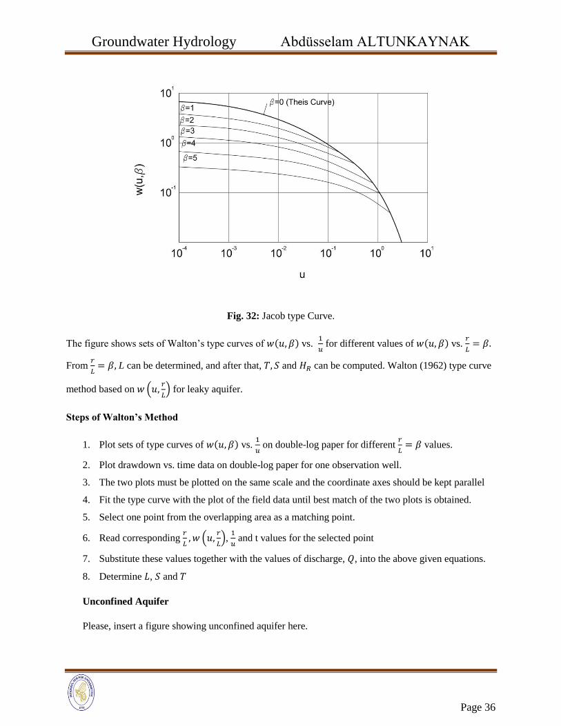
Fig. 32: Jacob type Curve.

The figure shows sets of Walton’s type curves of 𝑤(𝑢, 𝛽) vs. 1

𝑢 for different values of 𝑤(𝑢, 𝛽) vs.

𝑟

𝐿= 𝛽.

From 𝑟

𝐿= 𝛽, L can be determined, and after that, 𝑇, 𝑆 and 𝐻𝑅 can be computed. Walton (1962) type curve

method based on 𝑤 (𝑢,𝑟

𝐿) for leaky aquifer.

Steps of Walton’s Method

1. Plot sets of type curves of 𝑤(𝑢, 𝛽) vs. 1

𝑢 on double-log paper for different

𝑟

𝐿= 𝛽 values.

2. Plot drawdown vs. time data on double-log paper for one observation well.

3. The two plots must be plotted on the same scale and the coordinate axes should be kept parallel

4. Fit the type curve with the plot of the field data until best match of the two plots is obtained.

5. Select one point from the overlapping area as a matching point.

6. Read corresponding 𝑟

𝐿, 𝑤 (𝑢,

𝑟

𝐿),

1

𝑢 and t values for the selected point

7. Substitute these values together with the values of discharge, 𝑄, into the above given equations.

8. Determine 𝐿, 𝑆 and 𝑇

Unconfined Aquifer

Please, insert a figure showing unconfined aquifer here.


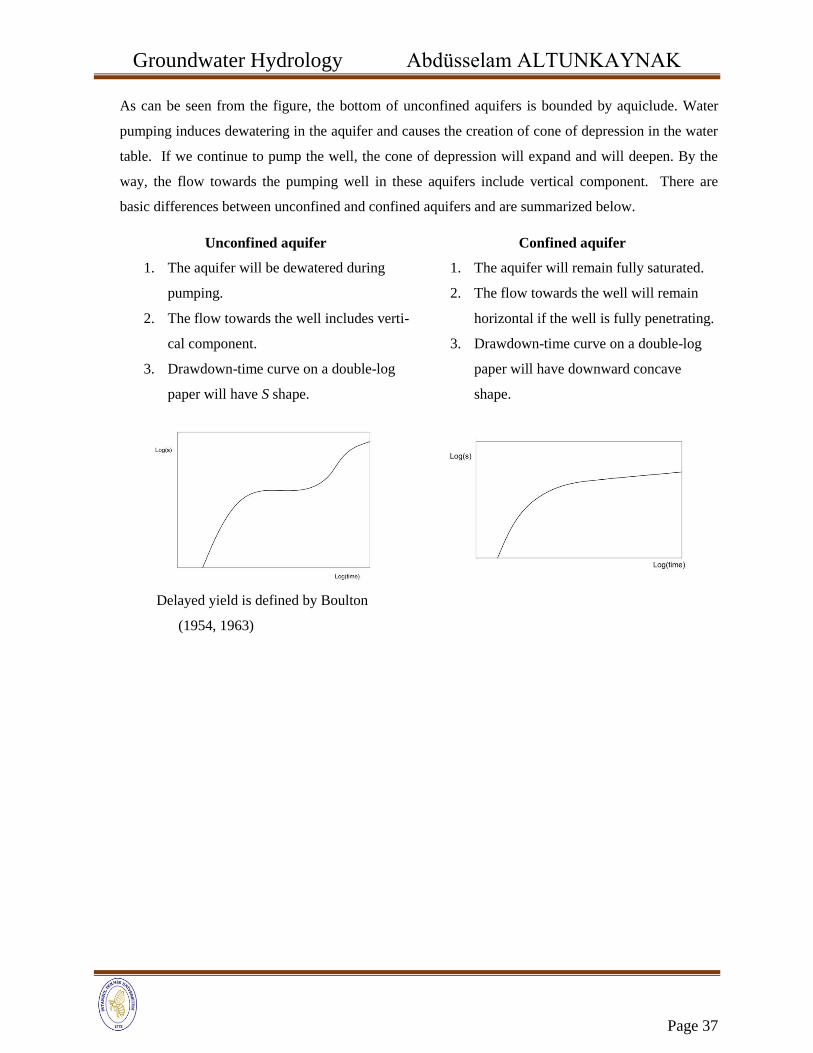
As can be seen from the figure, the bottom of unconfined aquifers is bounded by aquiclude. Water

pumping induces dewatering in the aquifer and causes the creation of cone of depression in the water

table. If we continue to pump the well, the cone of depression will expand and will deepen. By the

way, the flow towards the pumping well in these aquifers include vertical component. There are

basic differences between unconfined and confined aquifers and are summarized below.

Unconfined aquifer Confined aquifer

1. The aquifer will be dewatered during

pumping.

2. The flow towards the well includes verti-

cal component.

3. Drawdown-time curve on a double-log

paper will have S shape.

Delayed yield is defined by Boulton

(1954, 1963)

1. The aquifer will remain fully saturated.

2. The flow towards the well will remain

horizontal if the well is fully penetrating.

3. Drawdown-time curve on a double-log

paper will have downward concave

shape.


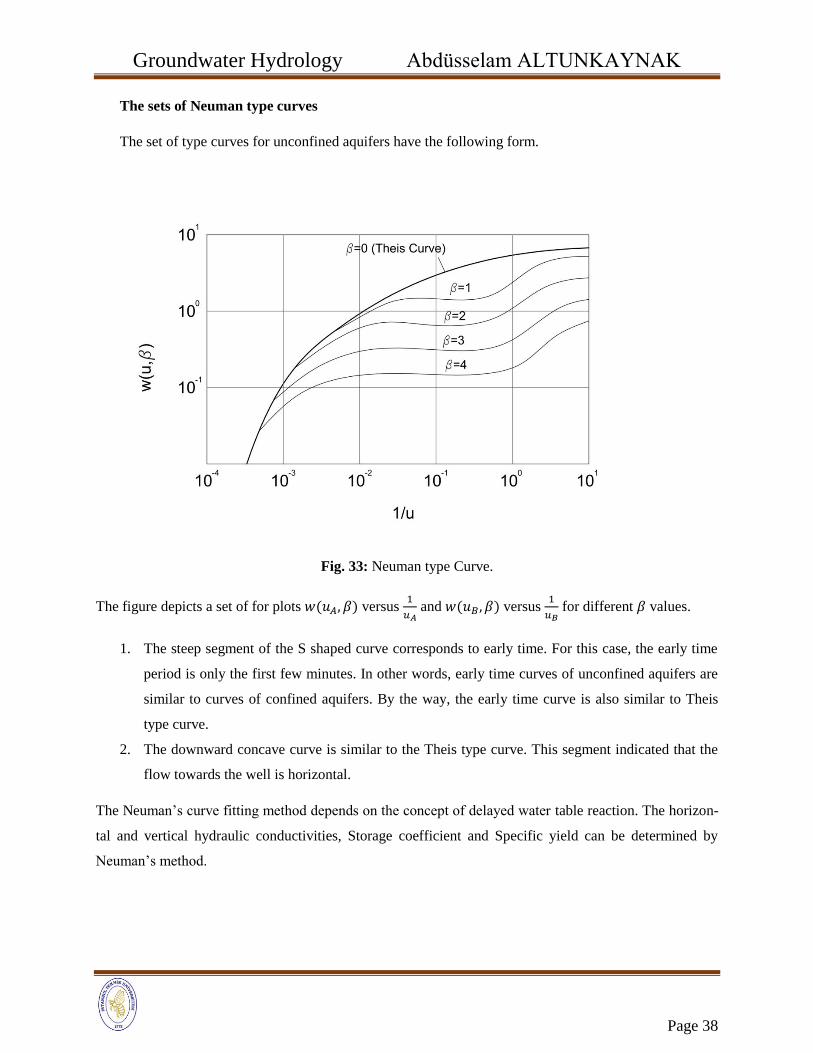
The sets of Neuman type curves

The set of type curves for unconfined aquifers have the following form.

Fig. 33: Neuman type Curve.

The figure depicts a set of for plots 𝑤(𝑢𝐴, 𝛽) versus 1

𝑢𝐴 and 𝑤(𝑢𝐵, 𝛽) versus

1

𝑢𝐵 for different 𝛽 values.

1. The steep segment of the S shaped curve corresponds to early time. For this case, the early time

period is only the first few minutes. In other words, early time curves of unconfined aquifers are

similar to curves of confined aquifers. By the way, the early time curve is also similar to Theis

type curve.

2. The downward concave curve is similar to the Theis type curve. This segment indicated that the

flow towards the well is horizontal.

The Neuman’s curve fitting method depends on the concept of delayed water table reaction. The horizon-

tal and vertical hydraulic conductivities, Storage coefficient and Specific yield can be determined by

Neuman’s method.


References

Bear, J. 1979. Hydraulics of groundwater. McGraw-Hill Book Co., New York, 567p

Boulton, N. S., 1954. The drawdown of the water table under non-steady conditions near a pumped well

in an unconfined formation, Proc. Inst. Civ. Eng., 3(3), 564-579.

Boulton, N. S., 1963. Analysis of data from nonequilibrium pumping tests allowing for delayed yield

from storage, Proc. Inst. Civil Eng., 26. 469-482.

Bouwer, H., 1978. Groundwater Hydrology. McGraw-Hill Book Co., New York, 480p

Cooper, N.N. and Jacob, C.E. 1946. A generalized graphical method for evaluating formation constant

and summarizing well field history. Trans., Am. Geophys. Un., 27, p.526-534.

De Glee, G.J. 1930. Over grondwaterstromingen bij teronttrekking door middle van putten. Thesis, J.

Waltman. Delft (The Netherlands), 175 p.

Dupuit, J. (1863). Estudes Théoriques et Pratiques sur le mouvement des Eaux dans les canaux décou-

verts et à travers les terrains perméables (Second Edition ed.). Paris: Dunod.

Fetter, C.W. 1980. Applied hydrogeology. Charles E. Merrill Publishing Co., 488 p

Forchheimer, P. (1886). "Über die Ergiebigkeit von Brunnen-Anlagen und Sickerschlitzen". Z. Archi-

tekt. Ing.-Ver. (Hannover) 32: 539–563.

Freeze, R.A. ve Cherry, J.A. 1979. Groundwater, Pearson, US.

Hantush, M.S. and Jacob, C.E. 1955. Non-steady radial flow in an infinite leaky aquifer. Trans. Am.

Geophys. Un., 36(1), p. 95-100.

Hantush, M.S. 1964. Hydraulics of wells, in Advances in Hydroscience (V. T. Chow, Ed.) Academic

Press, New York, 1, p. 281-442.

Kruseman, G.P., and Ridder, N.A., 1994. Analysis and evaluation of pumping test data. International

Institute for Land Reclamation and Improvement. Wageningen, The Netherlands, p73-97

Mariño, M.A. and Luthin, J.N. 1982. Seepage and groundwater: Developments in water science, 13.

Elsevier, Amsterdam, xvi + 490 pp

Marsily, G.D. 1986. Quantitative hydrogeology. Groundwater Hydrology for Engineers. Academic Press,

Inc., New York, 439p.

Neuman, S.P., 1975. Analysiso f pumpingt est data from anisotropic unconfined aquifers considering

delayed gravity response, Water Resour. Res., 11(2), 329-342.

http://en.wikipedia.org/wiki/Jules_Dupuit

http://en.wikipedia.org/wiki/Philipp_Forchheimer


Theis, C.V. 1935. The relation between lowering of the piezometric surface and rate and duration of dis-

charge of a well using ground water storage. Trans. Am. Geophys. Uni., 16th Annual Meeting, pt. 2,

p.519-524.

Thiem, G. (1906). "Hydrologische methoden" (in German). Leipzig: J. M. Gebhardt. p. 56

Todd, D.K., 1980. Groundwater Hydrology. John Wiley and Sons, New York, 535pp

Vedat Batu, 1998 Aquifer Hydraulics: A comprehensive guide to hydrogeologic data analysis, A Wiley-

Interscience Publication, JOHN WILEY & SONS, INC.

groundwater hydrology abdüsselam altunkaynak · groundwater hydrology abdüsselam altunkaynak page...

Documents