groundwater biodiversity conservation - state of oregon: state of
TRANSCRIPT
GROUNDWATER AND BIODIVERSITY
CONSERVATION:
A methods guide for integrating groundwater
needs of ecosystemsand species into
conservation plans in the Pacific Northwest
DECEMBER 2007
JENNY BROWNABBY WYERS
ALLISON ALDOUSLESLIE BACH
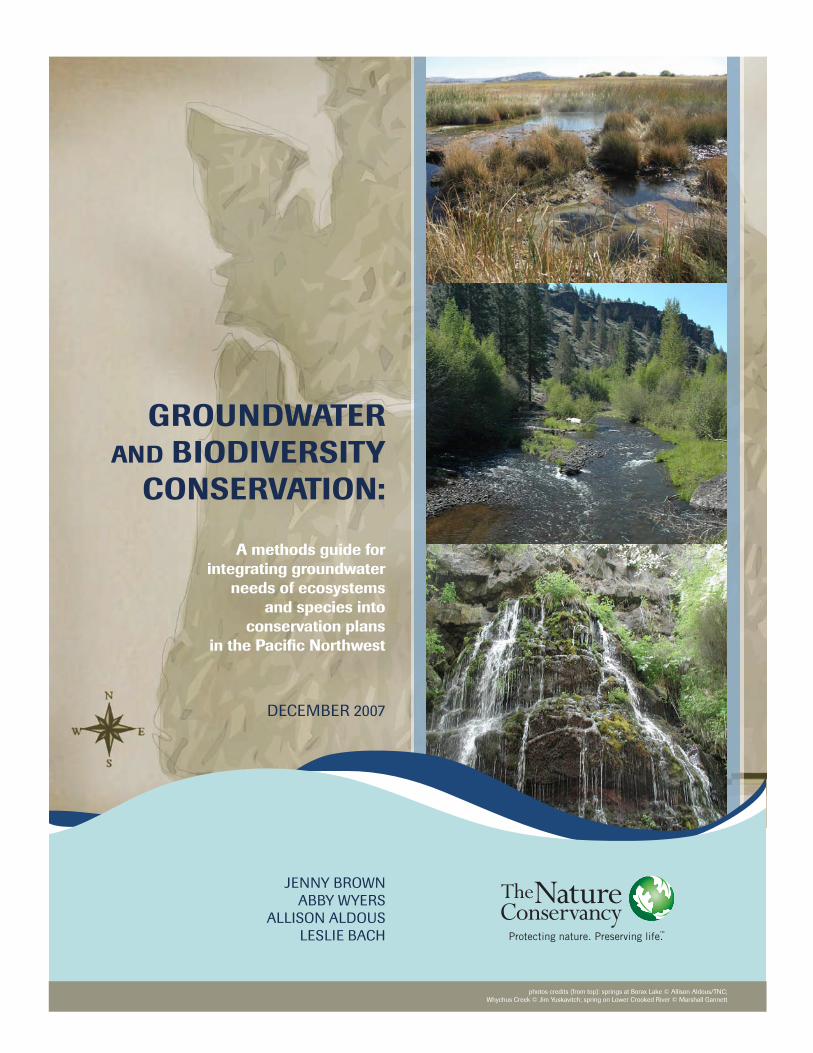
photos credits (from top): springs at Borax Lake © Allison Aldous/TNC; Whychus Creek © Jim Yuskavitch; spring on Lower Crooked River © Marshall Gannett

Acknowledgements: We are grateful to the Northwest Conservation Fund for financial support of this work. Additionally, this guide would not have been possible without the time and contributions of numerous colleagues. Our thanks goes to:
• Brad Nye (Deschutes Basin Land Trust) for field trip to Camp Polk to see springs and groundwater-dependent ecosystems of Whychus Creek drainage
• Colin Brown for retrieving literature from the Oregon State University library • Don Sada (Desert Research Institute) for review of KEAs for springs • Eloise Kendy (The Nature Conservancy) for review of earlier version of document • Jack Williams (Trout Unlimited) for review of KEAs for springs and Borax Lake chub
and review of document • James Newton for review of groundwater-dependent species in Whychus Ck • Jason Dedrick (Crooked River Watershed Council) for field trip to the Lower Crooked • Jen Newlin-Bell (The Nature Conservancy) for design of the cover • John Crandall (The Nature Conservancy) for field testing the methods guide at Moses
Coulee Conservation Area in WA • Jonathan Higgins (The Nature Conservancy) for review of KEAs for lakes and
discussions of methods development • Jonathan LaMarche (OR Water Resources Department) for review of earlier version of
document • Katharine Webster (University of Maine) for review of KEAs for lakes • Kathy Boomer (Smithsonian Institute) for review of earlier version of document • Laurie Morgan (WA Department of Ecology) for review of earlier version of document • Maret Pajutee (US Forest Service) for review of information on groundwater-dependent
biodiversity • Marshall Gannett (US Geological Survey) for help in understanding groundwater in the
Deschutes and for review of earlier versions of this document; • Michele Dephilip (The Nature Conservancy) for review of earlier version of document • Michelle McSwain (US BLM) for field trip to the Crooked River, discussion about
groundwater-dependent biodiversity, FLIR data for the Deschutes and Lower Crooked River, and for review of earlier version of this document;
• Mike Riehle (US Forest Service) for information on fish and stream temperatures in Whychus Creek
• Natalie Bennon (The Nature Conservancy) for formatting and proofreading • Paul Measeles (OR Department of Agriculture) for review of earlier version of document • Peter Skidmore (The Nature Conservancy) for review of earlier version of document • Robert Wiggington (The Nature Conservancy) for review of earlier version of document • Scott McCalou (Deschutes Resources Conservancy) for field trip to Alder Springs and
discussion of groundwater issues in the Whychus Creek drainage • Stephen Stanley (WA Department of Ecology) for review of earlier version of document • Steve Sebeysten (UC Berkeley) for help with KEAs and review of document • Tom Winter (US Geological Survey) for review of earlier version of document • Wendy Gerstel (consulting geologist) for review of earlier version of document
Groundwater Methods Guide Table of Contents
1
Table of contents Acknowledgements............................................................................................................................ 1. INTRODUCTION ....................................................................................................................... 4 2. GROUNDWATER BASICS, IN RELATION TO ECOSYSTEMS AND SPECIES....................... 9
2.1 Groundwater: ......................................................................................................................... 9 2.2 Water table........................................................................................................................... 10 2.3 Groundwater recharge: ........................................................................................................ 11 2.4 Groundwater discharge and availability to ecosystems:...................................................... 11 2.5 Groundwater movement ..................................................................................................... 14
3. IDENTIFYING AND MAPPING GROUNDWATER-DEPENDENT ECOSYSTEMS AND SPECIES ....................................................................................................................................... 16
3.1 Description of Groundwater-Dependent Ecosystems: ........................................................ 16 3.2 Overview of the importance of groundwater to biodiversity: ............................................. 17 3.3 Assessing the groundwater-dependence of specific ecosystems:........................................ 18
3.3.1. RIVERS:....................................................................................................................... 19 3.3.2. WETLANDS:............................................................................................................... 27 3.3.3. LAKES:........................................................................................................................ 39 3.3.4. SPRINGS: .................................................................................................................... 45 3.3.5. PHREATOPHYTIC ECOSYSTEMS:......................................................................... 49 3.3.6. CAVES:........................................................................................................................ 52
3.4 Identifying groundwater-dependent species:....................................................................... 53 3.5 Mapping GDEs .................................................................................................................... 58
4. DETERMINING GROUNDWATER REQUIREMENTS OF GDEs.......................................... 59 4.1 Groundwater key attribute ................................................................................................... 60 4.2 Measurable indicators of key attributes............................................................................... 60 4.3 Desired future condition of indicators ................................................................................. 60 4.4 Groundwater requirements of ecosystems........................................................................... 61
4.4.1. RIVERS:....................................................................................................................... 61 4.4.2. WETLANDS................................................................................................................ 65 4.4.3. LAKES......................................................................................................................... 69 4.4.4. SPRINGS: .................................................................................................................... 72 4.4.5. PHREATOPHYTIC ECOSYSTEMS.......................................................................... 75
4.5 Summary of groundwater requirements of ecosystems....................................................... 78 5. UNDERSTANDING GROUNDWATER FLOW SYSTEMS ...................................................... 83
5.1 The contributing area:.......................................................................................................... 83 5.2 Recharge areas:.................................................................................................................... 86 5.3 Groundwater Movement...................................................................................................... 97
5.3.1. Horizontal Flow Paths:................................................................................................. 97 5.3.2. Vertical flow paths: .................................................................................................... 101
6. SUMMARY.............................................................................................................................. 112 REFERENCES ............................................................................................................................ 113
Groundwater Methods Guide Table of Contents
2
Figures: 1-1 Overview of Methods ............................................................................................................... 7 1-2 Location of the Whychus Creek Watershed in the Deschutes Basin of Oregon ...................... 8 2-1 Unconfined and confined aquifers.......................................................................................... 10 2-2 Water table.............................................................................................................................. 10 2-3 View of groundwater flow showing movement of water from surface to substrate .............. 12 2-4 Conceptual effects of groundwater well on water available for discharge to ecosystems ..... 13 2-5 Generalized depiction of nested groundwater flow systems .................................................. 14 2-6 Example of nested flow paths for the eastern slope of Puget Sound...................................... 15 3-1 Decision tree to determine likelihood of groundwater dependence in river ecosystems ....... 20 3-2 Estimated baseflow at locations in Wash. where baseflow analysis complete (map) ........... 21 3-3 Temperature patterns in the streambed of gaining and losing river reaches .......................... 23 3-4 Groundwater-dependent river ecosystems of the Whychus Creek watershed (map)............. 24 3-5 Example use of the river ecosystem decision tree for Whychus Creek.................................. 25 3-6 Annual hydrograph for Whychus Creek................................................................................. 26 3-7 Gaining river reaches in Whychus Creek watershed (map) ................................................... 27 3-8 Decision tree to determine likelihood of groundwater-dependence in freshwater wetlands.. 30 3-9 Hydrogeologic setting common to groundwater discharge.................................................... 31 3-10 Groundwater discharging at surface as moves from permeable to less permeable deposit 32 3-11 Groundwater-dependent wetland ecosystems of the Whychus Creek watershed (map)...... 36 3-12 Example use of wetland ecosystem decision tree for Whychus Creek ................................ 38 3-13 Decision tree to determine likelihood of localor regional groundwater inputs to lakes....... 40 3-14 Groundwater-dependent lake ecosystems in the Whychus Creek watershed (map) ............ 42 3-15 Example use of lake ecosystem decision tree for Whychus Creek ...................................... 44 3-16 Hydrogeologic settings supporting spring formation ........................................................... 47 3-17 Springs of the Whychus Creek watershed (map) ................................................................. 48 3-18 Potentially groundwater-dependent phreatophytic upland ecosystems in Whychus (map) . 51 3-19 Known locations of groundwater-dependent species of Whychus Creek watershed (map) 55 3-20 GDEs of the Whychus Creek watershed (map).................................................................... 58 4-1 Overview of the steps for identifying groundwater requirements of ecosystems, species..... 59 4-2 Karst deposits in U.S. (map)................................................................................................... 65 4-3 Flow chart indicating likely effects on vegetation of a dropping water table ........................ 77 5-1 Topography of Deschutes Basin and Whychus Creek watershed (map)................................ 84 5-2 General geology of the Deschutes Basin and Whychus Creek watershed (map)................... 85 5-3 Surficial geologic deposits with relatively high permeability in the Deschutes Basin (map) 89 5-4 Refined map of the permeability of surficial geologic deposits in Whychus Creek .............. 90 5-5 Precipitation isoheytals in Whychus Creek watershed (map) ................................................ 91 5-6 Recharge areas predicted by GIS analysis for Whychus Creek watershed (map).................. 92 5-7 Mean annual recharge from infiltration of precipitation 93-95 Whychus (map) ................... 93 5-8 Correspondence of recharge areas predicted by GIS analysis and USGS model (map) ........ 94 5-9 Base map for the Whychus Creek watershed ........................................................................ .99 5-10 Map of intermediate and local groundwater flow lines in Whychus Creek watershed...... 100 5-11Location of transect under which hydrogeologic cross section was developed (map) ....... 102 5-12 Outline of Whychus Creek hydrogeologic cross section along transect A-A .................... 105 5-13 Addition of rivers and springs to Whychus Creek hydrogeologic cross section................ 106 5-14 Addition of geologic deposits to Whychus Creek hydrogeologic cross section ................ 107
Groundwater Methods Guide Table of Contents
3
5-15 Addition of recharge areas to Whychus Creek hydrogeologic cross section ..................... 108 5-16 Addition of intermediate and local flow lines to Whychus hydrogeologic cross section .. 110 Tables: 3-1 Documented phreatophytes that occur in the Pacific Northwest............................................ 49 3-2 Groundwater-dependent species of Conservation Concern in Whychus Creek watershed.... 56 4-1 Role of groundwater inputs to river ecosystems in different seasons .................................... 61 4-2 Key ecological attributes associated with groundwater; indicators of river integrity ............ 62 4-3 Key ecological attributes associated with groundwater; indicators of wetland integrity ....... 66 4-4 Key ecological attributes associated with groundwater; indicators of lake integrity ............. 69 4-5 Key ecological attributes associated with groundwater; indicators of spring integrity.......... 72 4-6 Key ecological attributes associated w/ groudnwater; phreatophytic ecosystem integrity .... 76 4-7 Summary: Key ecological attributes supported by groundwater; measurable indicators ...... 78 4-8 Key ecological attributes, indicators and desired future conditions in Whychus Creek ........ 80 5-1 High permeability geologic deposits in the Whychus Creek watershed ................................ 88 Appendices: A – GIS data sources and analyses for Whychus Creek B – Monitoring wetland hydrology using wells C – Water budgets D – Tools for understanding groundwater and biodiversity E – Evaluating the permeability of geologic deposits F – KEAs and indicators for groundwater-dependent species G – Glossary
Groundwater Methods Guide Section 1 Introduction
4
1. INTRODUCTION It is estimated that groundwater1 represents about 21 percent of the world’s fresh water and 97 percent of all the unfrozen fresh water on earth (Dunne and Leopold, 1978). Next to glaciers and ice caps, groundwater reservoirs are the largest holding basins for fresh water in the world’s hydrologic cycle. This large supply of water is critical to sustaining both ecological and human communities around the world. Groundwater is critically important to ecosystems and species across the Pacific Northwest. Rivers and streams throughout the region depend on groundwater for baseflow or cool water inputs, and many wetlands and most lakes are directly connected to groundwater (Brown et al., 2007; Sinclair and Pitz, 1999). The thousands of springs distributed throughout the region all depend on groundwater for their water supply. In Oregon, over 130 species of conservation concern have been identified as groundwater dependent, with groundwater providing either the hydrologic or water quality (including thermal) conditions they require (Brown et al., 2007). In most parts of the world, groundwater is perhaps equally important to humans – between 1.5 billion and 2.75 billion people rely on groundwater for their drinking water (Sampat, 2000). In the Pacific Northwest, groundwater is an important source of water for sustaining human populations. Groundwater is used for over 50 percent of irrigated agriculture, and over 40 percent of the total population and more than 90 percent of rural residents use groundwater for their drinking water (Oregon Department of Environmental Quality, 2003; Groundwater Protection Council, 2007). As a result, many of the same issues regarding the availability and quality of groundwater pertain to both human and ecological communities. Groundwater extraction and contamination have been identified as critical threats to the environment and biodiversity around the world (e.g. Stromberg et al., 1996; Alley and Leake, 2004; Carlton, 2006; Eamus et al., 2006), and these issues are mirrored in the Pacific Northwest. In many parts of the region, the demand for groundwater already exceeds supply (Oregon Water Resources Department, 2007). This situation is likely to intensify as population growth of over 25 percent is expected in some largely rural areas over the next fifteen years (Oregon Office of Economic Analysis, 2007). In addition, surface water supplies in the region have been fully allocated for use, thus water management agencies and water users are increasingly turning to groundwater to meet future water needs (Gannett et al., 2007; Oregon Water Resources Department Strategic Outlook, 2007). Furthermore, groundwater in several parts of this region fails to meet drinking water standards (Oregon Department of Environmental Quality, 2003). Recent studies indicate that groundwater contamination by nutrients or chemicals from agricultural, waste disposal and industrial operations (Jones and Wagner, 1995; Wentz et al., 1998) is prevalent, and many additional areas likely are susceptible to future contamination. Consequently, groundwater depletion and contamination pose a looming and potentially widespread threat to aquatic ecosystems in this region. Conservation of biodiversity that depends on groundwater requires developing strategies that allow for the use of groundwater in a way that is compatible with the persistence of these species and ecosystems. Development of these strategies must be based on an understanding of: 1) species and ecosystems that depend on groundwater; 2) how this biodiversity depends on
Groundwater Methods Guide Section 1 Introduction
5
groundwater; 3) the extent, source and movement of the groundwater; and 4) how alterations in the amount and quality of groundwater affect groundwater-dependent biodiversity. Successful conservation of any element of biodiversity (i.e. ecosystems, community, or species) requires completion of six steps (Margules and Pressey, 2000; Groves, 2003; Kernohan and Haufler, 1999):
1. Identification and mapping of the biodiversity 2. Description of the ecological requirements of this biodiversity 3. Identification of clear and measurable criteria that describe these requirements 4. Assessment of those activities or conditions in the surrounding landscape that threaten to
degrade the biodiversity by preventing these ecological requirements from being met 5. Identification, design, and implementation of strategies that can abate these threats 6. Monitoring the successes and failures of these strategies to ensure the ecological
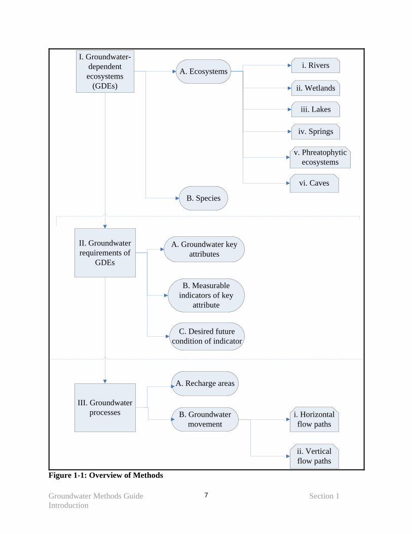
objectives, and thus the ecological requirements, are met. Completing these steps for groundwater-dependent biodiversity has proven difficult at times. Groundwater flow paths are often complex; data and information are limited, difficult to collect, and highly technical; and in-depth study and analysis can be expensive. Very few tools are available to assist in the development of effective conservation plans for ecosystems and species that depend upon groundwater, and no broadly applicable or efficient methodology has been developed to identify the linkages between this biodiversity and the patterns of groundwater systems. This Methods Guide is designed to fill this gap and to assist resource managers and planners in developing and implementing plans to conserve groundwater-dependent biodiversity. It provides tools and resources that will be valuable to those with no technical training in groundwater hydrology or hydrogeology, as well as to those with technical training in the subject. This Methods Guide will assist in the process of determining when and where groundwater is important for the protection and conservation of ecosystems and species. In addition, it provides steps that will begin to describe the groundwater system so that activities that are likely to affect groundwater-dependent biodiversity can be identified. The specific steps outlined in this guide are to (Figure 1-1):
1. Identify and map ecosystems and species that depend on groundwater (termed groundwater-dependent ecosystems, or GDEs)
2. Determine the groundwater requirements of these ecosystems and species and establish desired future conditions (or management objectives) to ensure these groundwater requirements are met
3. Develop an initial picture of groundwater hydrology at a particular site so that a first-cut can be made at identifying the areas that are integral to supporting GDEs and evaluating activities that threaten the quality and quantity of groundwater.
The overall framework presented in this methods guide is broadly applicable; however, the specific details provided were developed for use in the Pacific Northwest region of the United Sates. After a brief overview of groundwater basics as they relate to biodiversity conservation, this document leads the reader through the completion of the three tasks described above.

Groundwater Methods Guide Section 1 Introduction
6
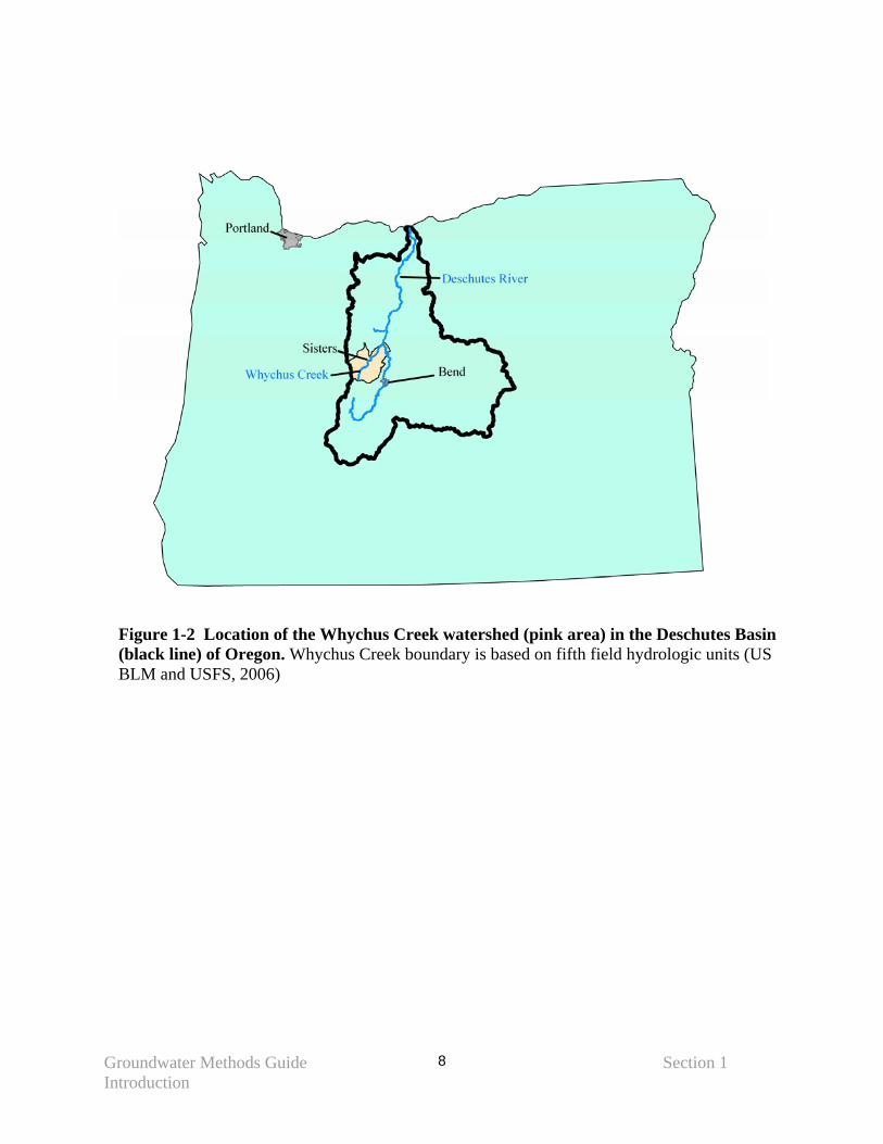
Throughout the discussion, each of these tasks, and their component steps, are illustrated with an example from the Whychus Creek (formerly Squaw Creek) watershed in the Upper Deschutes Basin of Oregon (Figure 1-2). These examples are provided in gray boxes, separated from the main text. Appendix A lists the datasets used in these analyses. Appendices B through F contain more detailed discussions of the tools and analyses presented in the guide. Appendix G is a glossary containing definitions for all terms that are provided in bold text in the guide.
Groundwater Methods Guide Section 1 Introduction
7
I. Groundwater-dependent ecosystems
(GDEs)
II. Groundwater requirements of
GDEs
A. Ecosystems
B. Species
i. Rivers
ii. Wetlands
iii. Lakes
iv. Springs
v. Phreatophytic ecosystems
vi. Caves
A. Groundwater key attributes
B. Measurable indicators of key
attribute
C. Desired future condition of indicator
III. Groundwater processes
A. Recharge areas
B. Groundwater movement
i. Horizontal flow paths
ii. Vertical flow paths
Figure 1-1: Overview of Methods
Groundwater Methods Guide Section 1 Introduction
8
Figure 1-2 Location of the Whychus Creek watershed (pink area) in the Deschutes Basin (black line) of Oregon. Whychus Creek boundary is based on fifth field hydrologic units (US BLM and USFS, 2006)
Methods Guide Section 2 Groundwater Basics and Biodiversity
9
2. GROUNDWATER BASICS, IN RELATION TO ECOSYSTEMS AND SPECIES In the following discussion, we provide an overview of key groundwater concepts and their importance to ecosystems and species. For each concept we provide a definition, information on why it is important to biodiversity and the types of activities that impair or alter it. Three excellent websites provide good descriptions of groundwater and should be examined for further information:
1. Groundwater Stewardship in Oregon, a website developed by the Oregon State University Extension Service: http://groundwater.orst.edu/index.html
2. Groundwater Basics, a website developed by Marquette County Community Information Services in Michigan, based primarily on the book ‘What is Groundwater?’ by Lyle S. Raymond, Jr.: http://www.mqtinfo.org/planningeduc0019.asp
3. Groundwater Primer, developed by EPA’s Region 5 and Purdue University’s Agricultural and Biological Engineering Department: http://www.purdue.edu/dp/envirosoft/groundwater/src/title.htm
More technical information can be obtained from:
4. ‘Basic Groundwater Hydrology’, a USGS publication: http://pubs.usgs.gov/wsp/wsp2220/ .
5. The USGS website listing further technical references: http://water.usgs.gov/ogw/pubs/resources_external.pdf
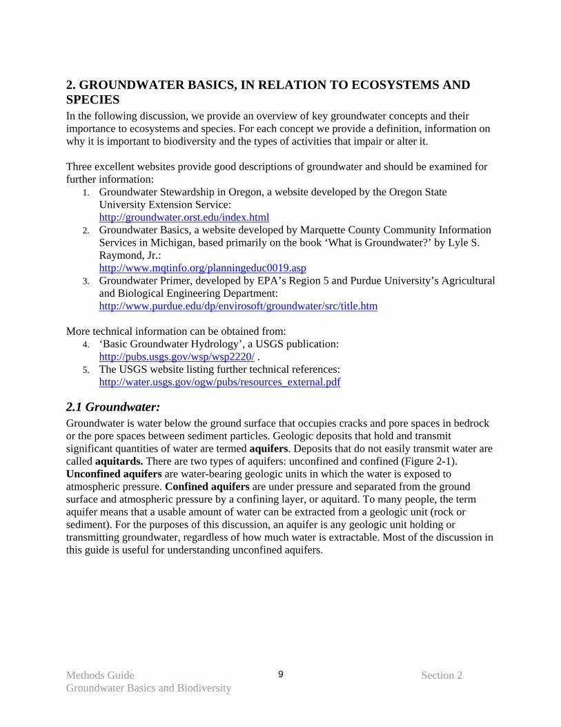
2.1 Groundwater: Groundwater is water below the ground surface that occupies cracks and pore spaces in bedrock or the pore spaces between sediment particles. Geologic deposits that hold and transmit significant quantities of water are termed aquifers. Deposits that do not easily transmit water are called aquitards. There are two types of aquifers: unconfined and confined (Figure 2-1). Unconfined aquifers are water-bearing geologic units in which the water is exposed to atmospheric pressure. Confined aquifers are under pressure and separated from the ground surface and atmospheric pressure by a confining layer, or aquitard. To many people, the term aquifer means that a usable amount of water can be extracted from a geologic unit (rock or sediment). For the purposes of this discussion, an aquifer is any geologic unit holding or transmitting groundwater, regardless of how much water is extractable. Most of the discussion in this guide is useful for understanding unconfined aquifers.
Methods Guide Section 2 Groundwater Basics and Biodiversity
10
Figure 2-1: Unconfined (diagonal lines) and confined (cross hatching) aquifers. Unconfined aquifers are not separated from the ground surface (or atmospheric pressure) by a confining layer (or aquitard), whereas confined aquifers are separated from the ground surface (or atmospheric pressure) by a confining layer.
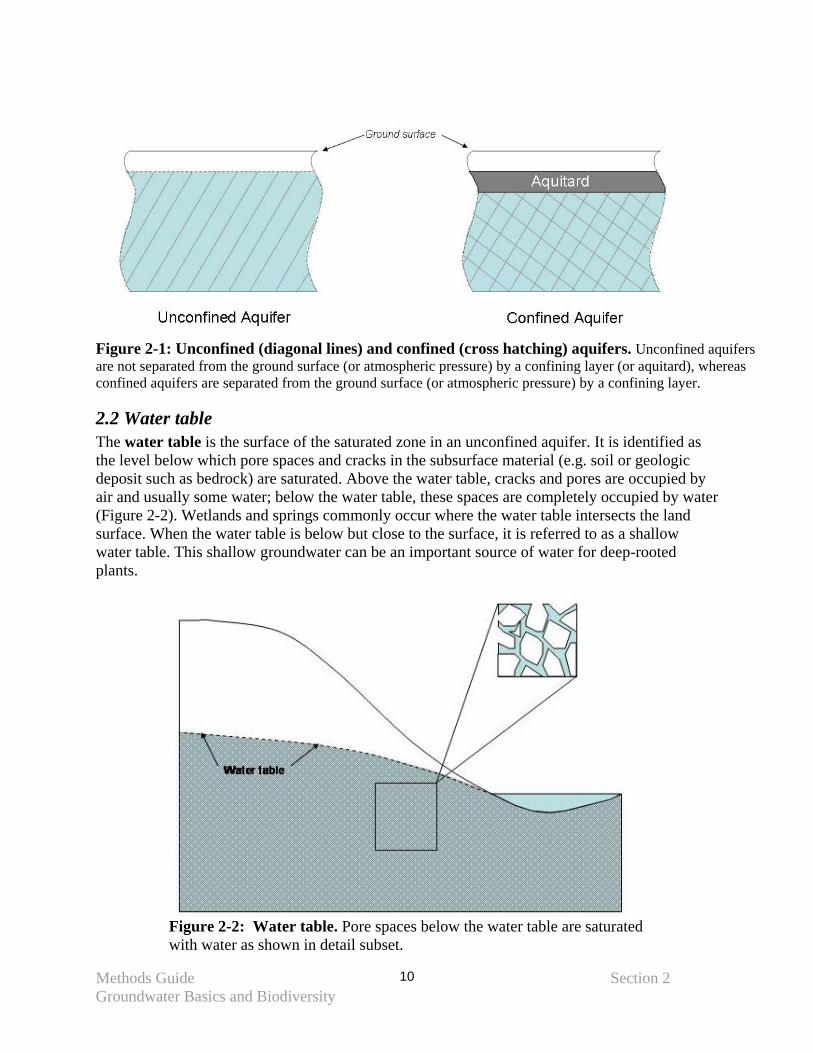
2.2 Water table The water table is the surface of the saturated zone in an unconfined aquifer. It is identified as the level below which pore spaces and cracks in the subsurface material (e.g. soil or geologic deposit such as bedrock) are saturated. Above the water table, cracks and pores are occupied by air and usually some water; below the water table, these spaces are completely occupied by water (Figure 2-2). Wetlands and springs commonly occur where the water table intersects the land surface. When the water table is below but close to the surface, it is referred to as a shallow water table. This shallow groundwater can be an important source of water for deep-rooted plants.
Figure 2-2: Water table. Pore spaces below the water table are saturated with water as shown in detail subset.
Methods Guide Section 2 Groundwater Basics and Biodiversity
11
2.3 Groundwater recharge: Groundwater is resupplied through the process of recharge. This generally occurs during precipitation or snowmelt, or when other surface input of water (e.g. a lake, river, wetland, or leaky irrigation canal) infiltrates into the soil column and then percolates into the underlying rock or surficial geologic deposit. The capacity of a particular area on the landscape to play a significant role in recharging groundwater is a function of the permeability of the soil, permeability of the underlying surficial geologic deposits, and the net amount of precipitation. The process of groundwater recharge is fundamental to ensuring that adequate supplies of groundwater are available to ecosystems and species. Human activities that reduce the infiltration capacity of soils or permeability of geologic deposits can reduce the recharge of groundwater. Examples of these activities may include construction of impervious surfaces such as roads, buildings, or parking lots. Additionally, conditions in groundwater recharge areas are fundamental to determining the quality of groundwater that is available to ecosystems and species. Because recharge areas are generally permeable, allowing water to move easily from the surface into the subsurface, these areas are where groundwater is most vulnerable to contamination. Land uses associated with groundwater contamination by nutrients (e.g. septic systems and fertilizers), toxins (e.g. underground injection wells, spills, and leaky underground storage tanks), and bacteria (e.g. septic systems) can impair groundwater quality if they are located in recharge areas.
2.4 Groundwater discharge and availability to ecosystems: Groundwater generally reaches ecosystems in two types of places:
1. Where subsurface water emerges at the land surface: At these locations, groundwater provides water to aquatic ecosystems such as springs, lakes, rivers, or wetlands. Groundwater can discharge in a concentrated area (e.g. at a spring), or it can seep to the surface in a dispersed manner. Groundwater discharge can also occur under the surface of a lake or stream where it is often not observed or measured.
2. Where plants extend roots into water in the saturated zones of unconfined aquifers:
When the water table reaches a depth near that accessible to plant roots, groundwater is then available for transpiration by phreatophytic vegetation.
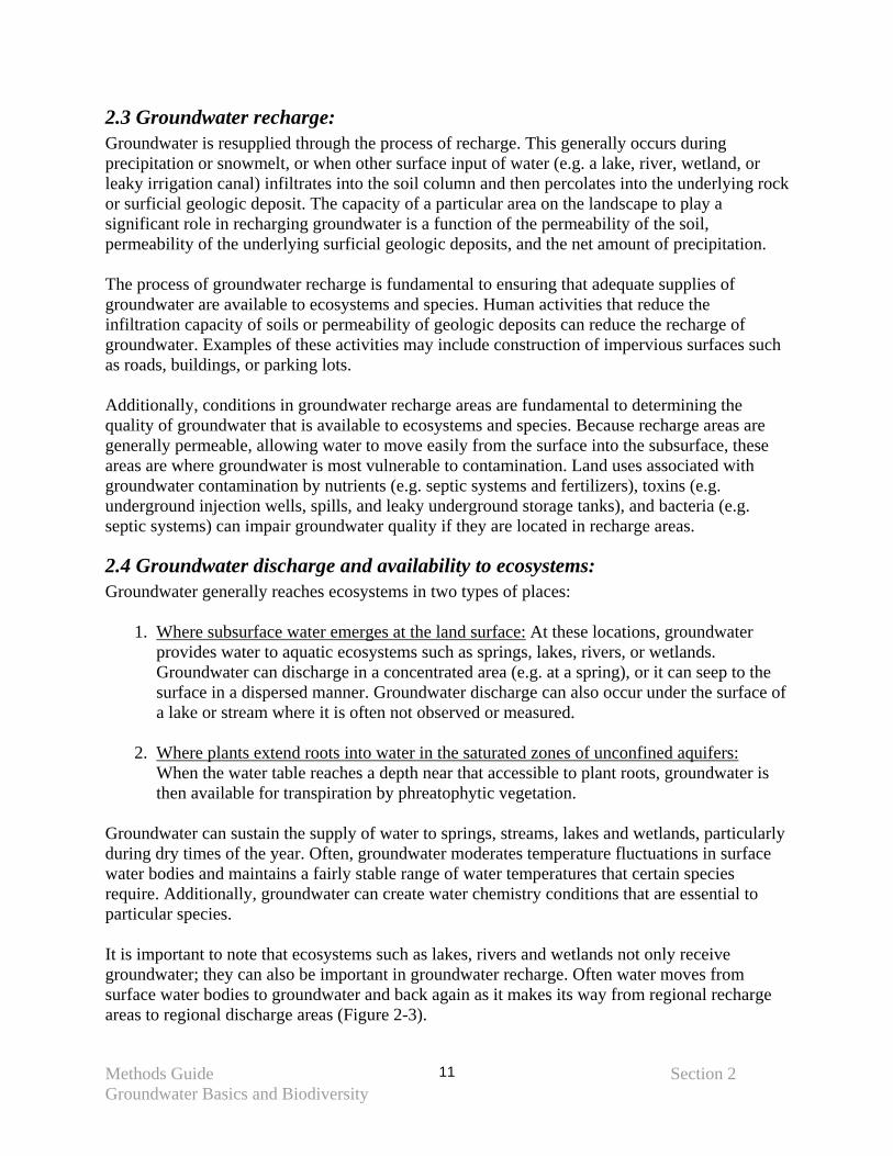
Groundwater can sustain the supply of water to springs, streams, lakes and wetlands, particularly during dry times of the year. Often, groundwater moderates temperature fluctuations in surface water bodies and maintains a fairly stable range of water temperatures that certain species require. Additionally, groundwater can create water chemistry conditions that are essential to particular species. It is important to note that ecosystems such as lakes, rivers and wetlands not only receive groundwater; they can also be important in groundwater recharge. Often water moves from surface water bodies to groundwater and back again as it makes its way from regional recharge areas to regional discharge areas (Figure 2-3).
Methods Guide Section 2 Groundwater Basics and Biodiversity
12
Figure 2-3 Generalized view of groundwater flow showing repeated movement of water from the surface to subsurface as it moves down gradient. With permission from Winter et al., 1998.
The magnitude of groundwater discharge is affected by the amount of groundwater recharged and the amount of groundwater extracted (e.g. by pumping of groundwater from wells or by extraction by vegetation). If recharge is reduced by human activities or if groundwater extraction exceeds natural recharge, less groundwater will be available to streams, wetlands and lakes.
Methods Guide Section 2 Groundwater Basics and Biodiversity
13
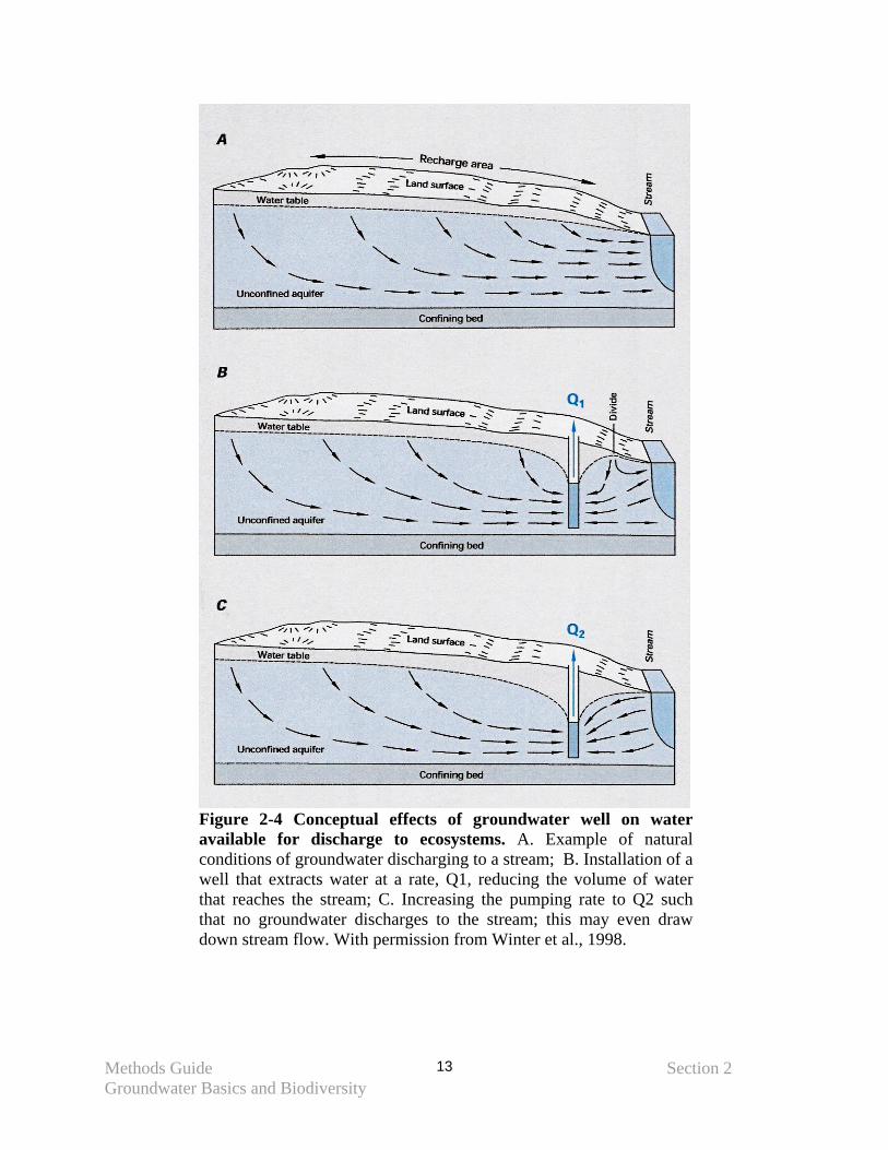
Figure 2-4 Conceptual effects of groundwater well on water available for discharge to ecosystems. A. Example of natural conditions of groundwater discharging to a stream; B. Installation of a well that extracts water at a rate, Q1, reducing the volume of water that reaches the stream; C. Increasing the pumping rate to Q2 such that no groundwater discharges to the stream; this may even draw down stream flow. With permission from Winter et al., 1998.
Methods Guide Section 2 Groundwater Basics and Biodiversity
14
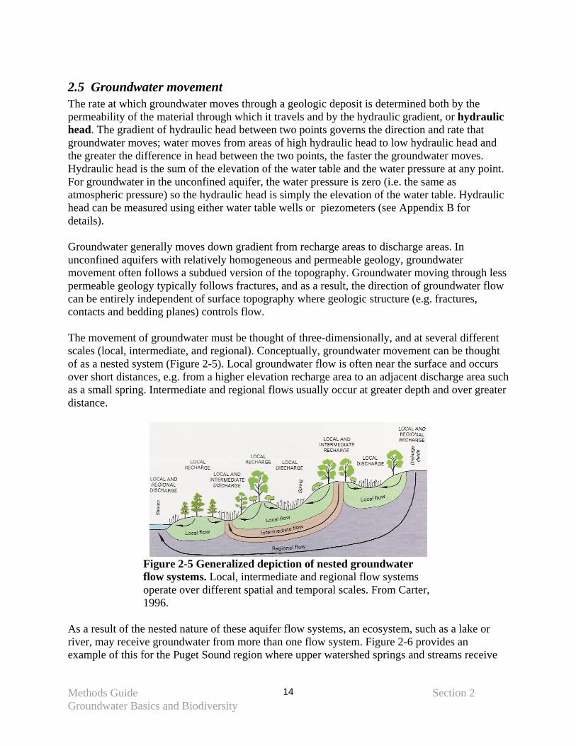
2.5 Groundwater movement The rate at which groundwater moves through a geologic deposit is determined both by the permeability of the material through which it travels and by the hydraulic gradient, or hydraulic head. The gradient of hydraulic head between two points governs the direction and rate that groundwater moves; water moves from areas of high hydraulic head to low hydraulic head and the greater the difference in head between the two points, the faster the groundwater moves. Hydraulic head is the sum of the elevation of the water table and the water pressure at any point. For groundwater in the unconfined aquifer, the water pressure is zero (i.e. the same as atmospheric pressure) so the hydraulic head is simply the elevation of the water table. Hydraulic head can be measured using either water table wells or piezometers (see Appendix B for details). Groundwater generally moves down gradient from recharge areas to discharge areas. In unconfined aquifers with relatively homogeneous and permeable geology, groundwater movement often follows a subdued version of the topography. Groundwater moving through less permeable geology typically follows fractures, and as a result, the direction of groundwater flow can be entirely independent of surface topography where geologic structure (e.g. fractures, contacts and bedding planes) controls flow. The movement of groundwater must be thought of three-dimensionally, and at several different scales (local, intermediate, and regional). Conceptually, groundwater movement can be thought of as a nested system (Figure 2-5). Local groundwater flow is often near the surface and occurs over short distances, e.g. from a higher elevation recharge area to an adjacent discharge area such as a small spring. Intermediate and regional flows usually occur at greater depth and over greater distance.
Figure 2-5 Generalized depiction of nested groundwater flow systems. Local, intermediate and regional flow systems operate over different spatial and temporal scales. From Carter, 1996.
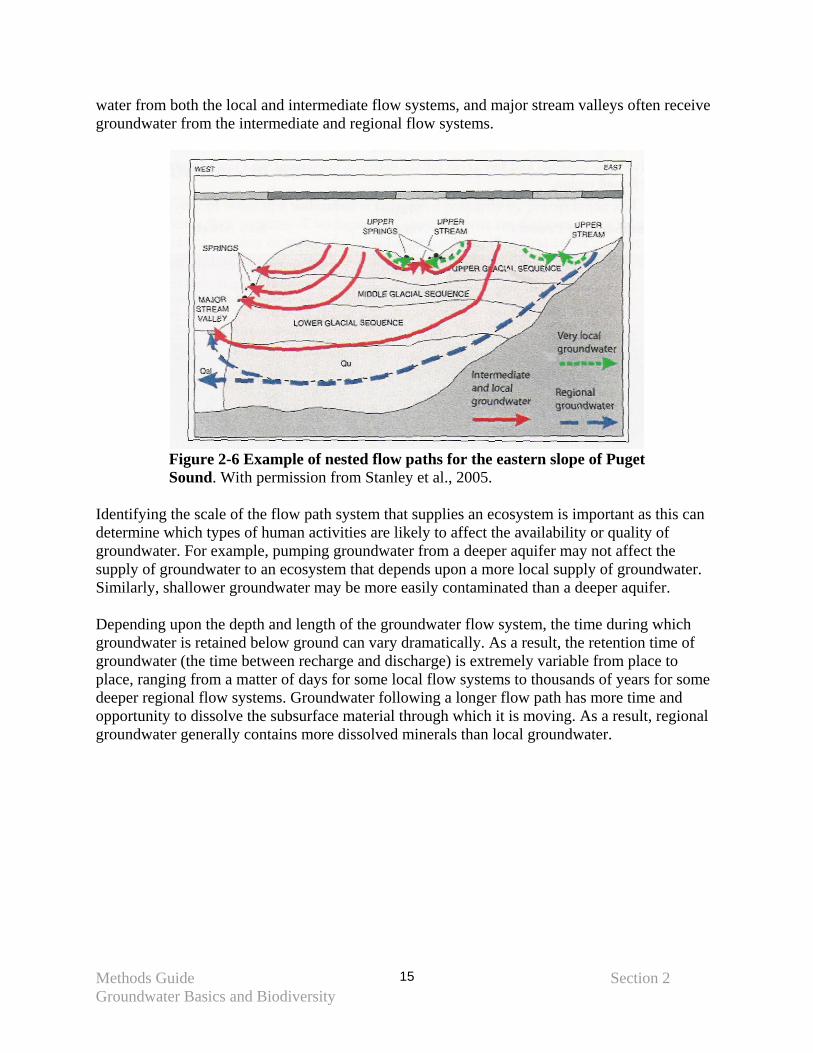
As a result of the nested nature of these aquifer flow systems, an ecosystem, such as a lake or river, may receive groundwater from more than one flow system. Figure 2-6 provides an example of this for the Puget Sound region where upper watershed springs and streams receive
Methods Guide Section 2 Groundwater Basics and Biodiversity
15
water from both the local and intermediate flow systems, and major stream valleys often receive groundwater from the intermediate and regional flow systems.
Figure 2-6 Example of nested flow paths for the eastern slope of Puget Sound. With permission from Stanley et al., 2005.
Identifying the scale of the flow path system that supplies an ecosystem is important as this can determine which types of human activities are likely to affect the availability or quality of groundwater. For example, pumping groundwater from a deeper aquifer may not affect the supply of groundwater to an ecosystem that depends upon a more local supply of groundwater. Similarly, shallower groundwater may be more easily contaminated than a deeper aquifer. Depending upon the depth and length of the groundwater flow system, the time during which groundwater is retained below ground can vary dramatically. As a result, the retention time of groundwater (the time between recharge and discharge) is extremely variable from place to place, ranging from a matter of days for some local flow systems to thousands of years for some deeper regional flow systems. Groundwater following a longer flow path has more time and opportunity to dissolve the subsurface material through which it is moving. As a result, regional groundwater generally contains more dissolved minerals than local groundwater.
Methods Guide 16 Section 3 Identifying groundwater-dependent ecosystems and species
3. IDENTIFYING AND MAPPING GROUNDWATER-DEPENDENT ECOSYSTEMS AND SPECIES
The first step in developing conservation plans for Groundwater-Dependent Ecosystems (GDEs) is to identify and map the ecosystems and species of conservation concern that depend upon groundwater. This section includes an overview of the ways in which GDEs depend upon groundwater, followed by guidance on identifying and mapping GDEs at the watershed scale. For further discussion on GDEs, see Eamus et al. (2006) and Eamus and Froend (2006). Before diving into a more detailed assessment of a particular conservation area and its ecosystems, it is often useful to get a general perspective on how water moves into and out of an area. This can easily be done by constructing a conceptual water budget for either the whole conservation area or a particular ecosystem. Appendix C provides guidance on developing and using a water budget.
3.1 Description of Groundwater-Dependent Ecosystems: Many ecosystems and species depend upon groundwater for some or all of their water supply. Some ecosystems, such as springs and certain rivers, lakes, and wetlands, depend on the actual discharge of groundwater at the surface. Other ecosystems, for example certain forests and riparian areas, depend upon the water table being relatively near the surface. Aquifer and subterranean ecosystems rely on the flow of groundwater below the surface. Researchers in Australia have identified three classes of ecosystems that depend upon groundwater (Eamus et al., 2006). We use these same classes as a basis for this discussion, with a few modifications:
1. Ecosystems that depend upon surface expressions of groundwater: We include rivers, lakes, wetlands, and springs in this category. While springs always depend upon groundwater, the groundwater-dependence of the other ecosystems is variable. Rivers, lakes, and wetlands may be groundwater-dependent if they occur in a hydrogeologic setting that is conducive to groundwater discharge. Section 3.4 provides guidance for determining if these conditions exist.
2. Above-ground ecosystems that depend upon sub-surface expressions of groundwater: We use the term ‘phreatophytic ecosystems’ to describe these ecosystems. The availability of groundwater to these ecosystems also depends upon their hydrogeologic setting.
3. Aquifer and cave ecosystems: In this document, we focus on cave ecosystems which, if wet, always depend upon groundwater.
Several sources of information can be used to identify ecosystems of conservation concern that could potentially depend upon groundwater. The Nature Conservancy (Conservancy) conducts ecoregional assessments to identify portfolios of sites where ecosystems and species are best conserved (Groves et al., 2000). The US Forest Service (USFS) produces watershed analyses that describe the hydrologic and biological components of Forest Service watersheds. Natural Heritage Program (NHP) databases list locations of ecosystems and species that are at risk. Finally, local experts and resource professionals can provide critical input to identifying ecosystems of concern.
Methods Guide 17 Section 3 Identifying groundwater-dependent ecosystems and species
3.2 Overview of the importance of groundwater to biodiversity: In general, there are three ecological attributes related to groundwater that can be important to GDEs:
1. Quantity, timing, location, and duration of water delivery: This is termed ‘hydrologic regime’ in the remainder of this document, but in conservation planning is often indicated by the hydrograph of rivers and hydroperiod of wetlands. Ecosystems can depend on groundwater for a significant portion of their water supply throughout the year or at certain times such as in the dry season. Some examples are: • rivers that have low but steady groundwater inflow and that depend on groundwater
for late season flow (baseflow) • wetlands, such as fens, that rely on groundwater for a large proportion of their water
supply • mesic forests, where tree roots near the shallow water table and use that groundwater
as a source of water, particularly during the dry season.
2. Water quality or specific water chemistry: This is termed ‘water chemistry’ in this document. When groundwater discharges at the surface, its chemical composition is a combination of the initial chemical conditions of the recharge water and the geologic materials through which the water travels. Groundwater moving through highly soluble geologic deposits will contain the minerals characteristics of this substrate. The longer groundwater remains in these deposits (i.e. the more slowly that it moves or the longer its flow path), the higher the concentrations of minerals. For example, calcium carbonate can dissolve from limestone and some glacial deposits into groundwater. A suite of ecosystems, harboring a unique flora and fauna, are specialized to the high pH and calcium concentrations associated with such groundwater (Almendinger and Leete, 1998a and b; Lower Columbia Fish Recovery Board, 2004).
3. Specific temperature conditions: Water temperature regimes – either cold or hot (termed
‘thermal’) – can be maintained by groundwater. In relatively shallow flow systems, groundwater temperature is approximately equal to the mean annual air temperature of the recharge area (Manga, 2001). If water begins its underground journey at high elevations, for example, where the mean annual air temperature is 7°C (45°F), it will maintain this temperature, emerging at 7°C at much lower elevations where the air and surface water temperatures are much warmer. This is particularly important for species such as salmonids, including bull trout, which have specific temperature requirements for spawning and egg incubation (USFWS, 2002; King County DNR, 2000).
In some settings, groundwater emerges at the surface as hot springs and is warm, not cold. This generally occurs if water circulates more deeply, often in regional flow systems, where it is heated prior to discharge (Ingebritsen et al., 1989; Evans et al., 2002). Groundwater does not need to move very deeply to be heated by geothermal gradients; on average, the temperature of the earth’s crust increases 30°C (86°F) for every kilometer in depth. This means that to raise the temperature of groundwater 7 °C (20°F) above the mean air temperature of the recharge area, the water only needs to move 230 m (754 ft) below the surface. The microbial and invertebrate flora of hot springs are quite sensitive to water temperature changes as are fauna such as the Borax Lake chub (Sada,
Methods Guide 18 Section 3 Identifying groundwater-dependent ecosystems and species
unpublished; Sompong et al., 2005; Breitbart et al., 2004; Wingard et al., 1996; USFWS, 2006; De Jong et al., 2005). Groundwater emerging at the surface often maintains a fairly constant temperature year round. This low variability can be important as groundwater-dependent species may be adapted to these stable conditions. Furthermore, the constant temperature can be important in colder environments or seasons as, even though it is not ‘warm’, the groundwater is warmer than the surrounding air temperature and is less prone to freezing. Groundwater discharge areas can be important for maintaining ice-free conditions in aquatic ecosystems.
3.3 Assessing the groundwater-dependence of specific ecosystems: This section provides guidance on locating and mapping occurrences of six different ecosystems and evaluating their groundwater dependence. The six ecosystems are subdivided from the three classes of ecosystems listed in section 3.1. Rivers, wetlands, lakes and springs, fall within class 1, ecosystems that depend upon surface expressions of groundwater; phreatophytic ecosystems fall within class 2, above-ground ecosystems that depend upon sub-surface expressions of groundwater; and caves fall within class 3, aquifer and subterranean ecosystems A key driver controlling the significance of groundwater to any given ecosystem is the hydrogeologic setting. Information is provided to assess the hydrogeologic setting of specific occurrences of each of the six ecosystems as well as to assess other indicators of groundwater dependence. Evaluation of each ecosystem is illustrated using the Whychus Creek example.
Hydrogeologic setting: The hydrogeologic setting is defined by factors that control the flow of surface and ground water to ecosystems. These factors include (Winter, 1988; Komor, 1994; Bedford, 1999):
(a) topography (elevation) and slope of the land surface in the watershed (b) composition, stratigraphy, and structure of subsurface geological materials in
the watershed and underlying the ecosystem (c) porosity and depth of geologic materials underlying and adjacent to the
ecosystem, and (d) position of the ecosystem in the landscape with respect to surface- and
groundwater flow systems. In addition, climate controls precipitation and evapotranspiration within the watershed and ecosystem (Winter, 1992). Together these factors determine the relative importance of different water inputs and outputs in an ecosystem’s water budget (Brinson, 1993). As a consequence, they play the major role in controlling the extent and seasonal patterns in water table fluctuations, direction and velocity of water flows, and water chemistry (Winter et al., 1998).
Methods Guide 19 Section 3 Identifying groundwater-dependent ecosystems and species RIVERS
3.3.1. Assessing the groundwater-dependence of specific ecosystems: RIVERS
3.3.1.1. Identifying and mapping river ecosystems: Rivers of conservation concern can be identified using the freshwater classification of the Conservancy’s ecoregional assessments and information from USFS watershed analysis documents. Once identified, they can be located and mapped by examining local topographic maps or using one of the following hydrography datasets:
o National Hydrography Dataset PLUS - 1:100,000 (USGS, 2005) http://www.horizon-systems.com/nhdplus/drainage-area.htm
o Pacific Northwest Hydrography Framework Clearinghouse - Water courses data
available at: http://hydro.reo.gov/index.html
3.3.1.2. Evaluating the importance of groundwater to river ecosystems: Most rivers or streams are likely to receive some of their flow from groundwater at various times of the year, but the importance of groundwater to the overall flow system varies from river to river. For conservation planning purposes, the groundwater is important to a river ecosystem if:
1. It makes a significant contribution to annual stream flow, or 2. It maintains a particular component of streamflow, such as baseflow.
Four approaches, organized from simple to more complex, can be used to evaluate the importance of groundwater to a particular river ecosystem: the river ecosystem decision tree, analysis of streamflow data, seepage runs, and temperature studies.
3.3.1.2.A. River ecosystem decision tree: The decision tree below (Figure 3-1) provides some field indicators that can be used to identify the importance of groundwater to a natural (e.g. unregulated) river ecosystem. A series of sequential questions are asked, and answered, to provide an initial assessment of the significance of groundwater to the hydrologic regime of a reach of stream or river. The decision tree begins with seasonal patterns of flow (Figure 3-1 Q1). Ephemeral and intermittent streams are, in general, dominated by surface runoff, although some intermittent streams can receive seasonal inputs from small springs (Gordon et al., 1993). It is important to note that management actions may have changed the seasonal patterns of flow. Some naturally perennial streams are currently intermittent due to diversions, and some naturally intermittent streams may be perennial due to changes such as dam operations. The decision tree should be considered for natural or unaltered systems. If the stream naturally flows year round, then the area near the stream should be searched for springs (Q2). Although the presence of one spring does not mean that a significant portion of flow is from groundwater, it does suggest that groundwater is reaching the stream and further analysis is necessary to evaluate its significance. A perennial stream, without springs, that is not supported by snowmelt from snowfields or glaciers (Q3) and that lacks significant summer precipitation (Q4) is most likely supported by subsurface groundwater. However,
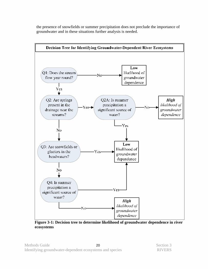
Methods Guide 20 Section 3 Identifying groundwater-dependent ecosystems and species RIVERS
the presence of snowfields or summer precipitation does not preclude the importance of groundwater and in these situations further analysis is needed.
Figure 3-1: Decision tree to determine likelihood of groundwater dependence in river ecosystems
Methods Guide 21 Section 3 Identifying groundwater-dependent ecosystems and species RIVERS
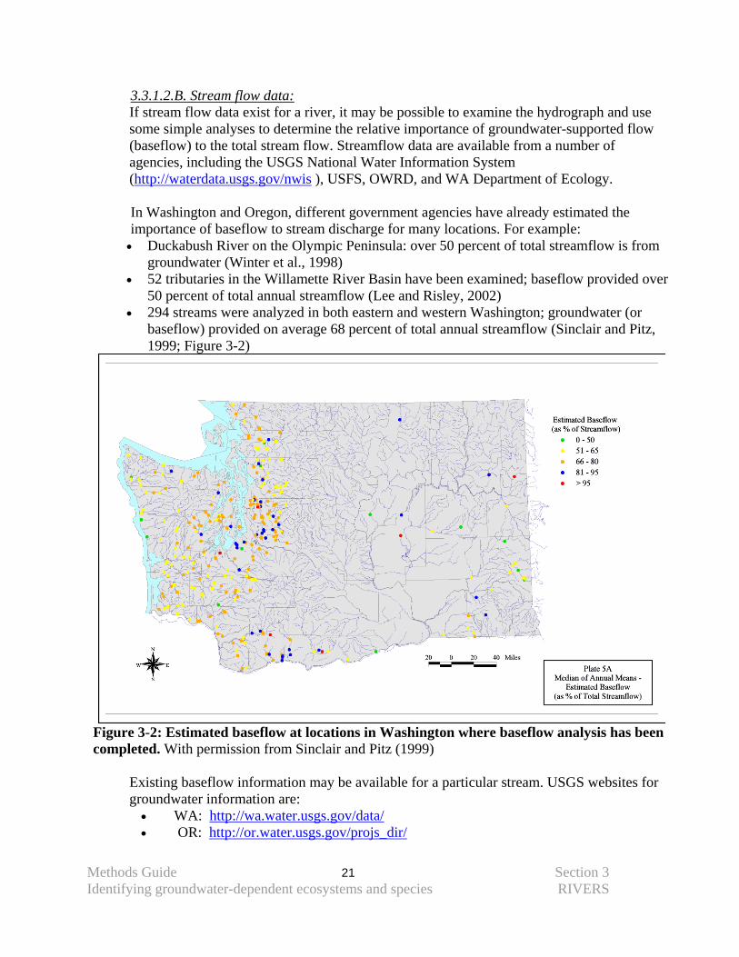
3.3.1.2.B. Stream flow data: If stream flow data exist for a river, it may be possible to examine the hydrograph and use some simple analyses to determine the relative importance of groundwater-supported flow (baseflow) to the total stream flow. Streamflow data are available from a number of agencies, including the USGS National Water Information System (http://waterdata.usgs.gov/nwis ), USFS, OWRD, and WA Department of Ecology. In Washington and Oregon, different government agencies have already estimated the importance of baseflow to stream discharge for many locations. For example: • Duckabush River on the Olympic Peninsula: over 50 percent of total streamflow is from
groundwater (Winter et al., 1998) • 52 tributaries in the Willamette River Basin have been examined; baseflow provided over
50 percent of total annual streamflow (Lee and Risley, 2002) • 294 streams were analyzed in both eastern and western Washington; groundwater (or
baseflow) provided on average 68 percent of total annual streamflow (Sinclair and Pitz, 1999; Figure 3-2)
Figure 3-2: Estimated baseflow at locations in Washington where baseflow analysis has been completed. With permission from Sinclair and Pitz (1999)
Existing baseflow information may be available for a particular stream. USGS websites for groundwater information are: • WA: http://wa.water.usgs.gov/data/ • OR: http://or.water.usgs.gov/projs_dir/
Methods Guide 22 Section 3 Identifying groundwater-dependent ecosystems and species RIVERS
In locations where these analyses have not already been conducted, an analysis of the mean monthly flows may be useful. This involves a comparison of the low flow to the annual mean monthly flow at a particular site; if the low flow is a large percentage of the mean monthly flow, then groundwater is more likely to be an important component of water supply for the stream. More detailed analyses can be conducted using such software as HYSEP, developed by the USGS (Sloto and Crouse, 1996; http://water.usgs.gov/software/hysep.html ), provided that daily mean stream discharge data exist. Appendix D has more details on data requirements and output from baseflow analysis of stream hydrograph data.
3.3.1.2.C. Seepage runs: Seepage runs consist of stream flow measurements made at several points along a stream or river at the same instant in time, along with an accounting of tributary inflows and diversions. These data can be used to identify whether groundwater is discharging to a stream reach (termed a ‘gaining reach’) or whether streamwater is recharging groundwater (termed a ‘losing reach’). These ‘gaining’ and ‘losing’ conditions can change throughout the year, although large gains or losses are generally less variable. For the purposes of identifying groundwater dependence, it is best to collect these data during the low flow season. Gaining reaches in the late summer or fall are evidence that groundwater is important to a stream. Appendix D summarizes how these data are collected and the information that they provide.
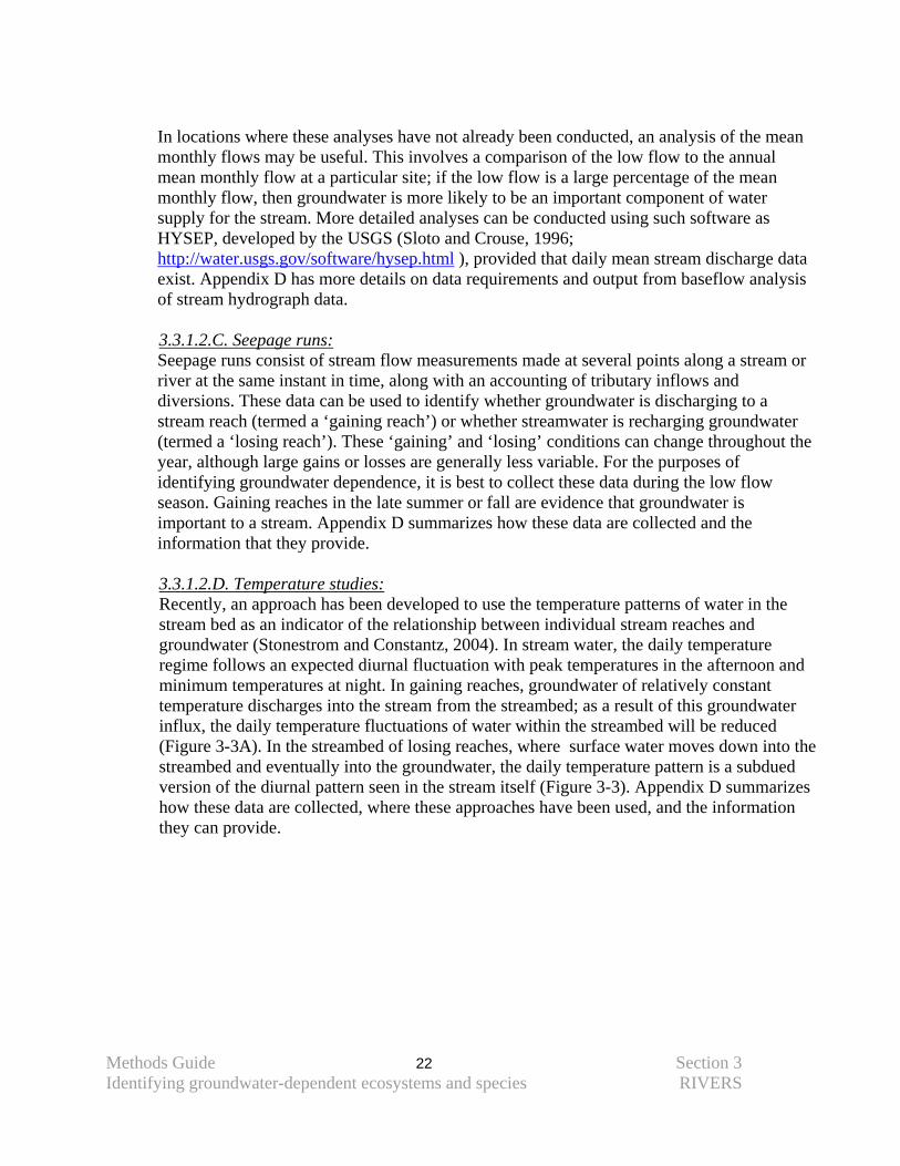
3.3.1.2.D. Temperature studies:
Recently, an approach has been developed to use the temperature patterns of water in the stream bed as an indicator of the relationship between individual stream reaches and groundwater (Stonestrom and Constantz, 2004). In stream water, the daily temperature regime follows an expected diurnal fluctuation with peak temperatures in the afternoon and minimum temperatures at night. In gaining reaches, groundwater of relatively constant temperature discharges into the stream from the streambed; as a result of this groundwater influx, the daily temperature fluctuations of water within the streambed will be reduced (Figure 3-3A). In the streambed of losing reaches, where surface water moves down into the streambed and eventually into the groundwater, the daily temperature pattern is a subdued version of the diurnal pattern seen in the stream itself (Figure 3-3). Appendix D summarizes how these data are collected, where these approaches have been used, and the information they can provide.
Methods Guide 23 Section 3 Identifying groundwater-dependent ecosystems and species RIVERS
Figure 3-3: Temperature patterns in the streambed of gaining and losing river reaches. A: Streambed temperatures of gaining reaches are relatively constant due to groundwater influxes. B: Streambed temperatures of losing reaches have subdued diurnal fluctuations. With permission from Stonestrom and Constantz, 2004.
A B
Methods Guide 24 Section 3 Identifying groundwater-dependent ecosystems and species RIVERS example
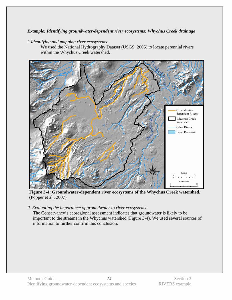
Example: Identifying groundwater-dependent river ecosystems: Whychus Creek drainage i. Identifying and mapping river ecosystems:
We used the National Hydrography Dataset (USGS, 2005) to locate perennial rivers within the Whychus Creek watershed.
Figure 3-4: Groundwater-dependent river ecosystems of the Whychus Creek watershed. (Popper et al., 2007).
ii. Evaluating the importance of groundwater to river ecosystems:
The Conservancy’s ecoregional assessment indicates that groundwater is likely to be important to the streams in the Whychus watershed (Figure 3-4). We used several sources of information to further confirm this conclusion.
Methods Guide 25 Section 3 Identifying groundwater-dependent ecosystems and species RIVERS example
Lowlikelihood of groundwater dependence
No
Yes
Highlikelihood of groundwater dependence
Yes
No
Low likelihood of groundwater dependence
Yes
No
Highlikelihood of groundwater dependence
No
Yes
Decision Tree for Identifying Groundwater Dependent River Ecosystems
No
Yes
Q1: Does the stream flow year round?
Q2: Are springs present in the
drainage near the streams?
Q2A: Is summer precipitation a
significant source of water?
Q3: Are snowfields or glaciers in the headwaters?
Q4: Is summer precipitation a
significant source of water?
Figure 3-5: Example use of the river ecosystem decision tree for Whychus Creek
• River ecosystem decision tree: Initially, we used the decision tree for rivers (Figure 3-5),
to assess the likelihood that groundwater was important to these streams, as follows:
Q1: Does the stream flow year round? Yes, according to local experts and existing gaging data, under natural conditions this stream flows year round, although it currently has dry periods due to water diversions.
Methods Guide 26 Section 3 Identifying groundwater-dependent ecosystems and species RIVERS example
Q2: Are springs present in the drainage near the stream? Yes. According to the USGS topo maps and people familiar with the stream, several large springs contribute water to the stream.
Q2A: Is summer precipitation a significant source of water? No. In eastern Oregon, summers are fairly dry and other than occasional thunderstorms, little precipitation occurs.
In summary, the perennial nature of the streams in this watershed, the prevalence of springs adjacent to the stream channels, and the absence of significant summer precipitation suggests that groundwater is likely an important source of water to these streams and that they are groundwater dependent.
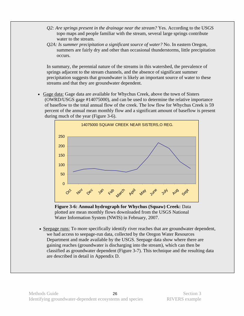
• Gage data: Gage data are available for Whychus Creek, above the town of Sisters
(OWRD/USGS gage #14075000), and can be used to determine the relative importance of baseflow to the total annual flow of the creek. The low flow for Whychus Creek is 59 percent of the annual mean monthly flow and a significant amount of baseflow is present during much of the year (Figure 3-6).
14075000 SQUAW CREEK NEAR SISTERS,O REG.
0
50
100
150
200
250
Oct NovDec
Jan
FebMarc
hApri
lMay
June Ju
lyAug
Sept
Figure 3-6: Annual hydrograph for Whychus (Squaw) Creek: Data plotted are mean monthly flows downloaded from the USGS National Water Information System (NWIS) in February, 2007.
• Seepage runs: To more specifically identify river reaches that are groundwater dependent,
we had access to seepage-run data, collected by the Oregon Water Resources Department and made available by the USGS. Seepage data show where there are gaining reaches (groundwater is discharging into the stream), which can then be classified as groundwater dependent (Figure 3-7). This technique and the resulting data are described in detail in Appendix D.
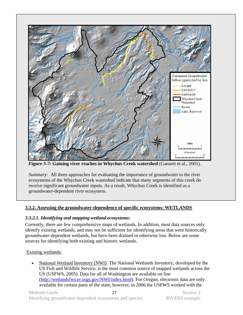
Methods Guide 27 Section 3 Identifying groundwater-dependent ecosystems and species RIVERS example
Figure 3-7: Gaining river reaches in Whychus Creek watershed (Gannett et al., 2001). Summary: All three approaches for evaluating the importance of groundwater to the river ecosystems of the Whychus Creek watershed indicate that many segments of this creek do receive significant groundwater inputs. As a result, Whychus Creek is identified as a groundwater-dependent river ecosystem.
3.3.2. Assessing the groundwater-dependence of specific ecosystems: WETLANDS
3.3.2.1. Identifying and mapping wetland ecosystems: Currently, there are few comprehensive maps of wetlands. In addition, most data sources only identify existing wetlands, and may not be sufficient for identifying areas that were historically groundwater-dependent wetlands, but have been drained or otherwise lost. Below are some sources for identifying both existing and historic wetlands. Existing wetlands:
• National Wetland Inventory (NWI): The National Wetlands Inventory, developed by the
US Fish and Wildlife Service, is the most common source of mapped wetlands across the US (USFWS, 2005). Data for all of Washington are available on line (http://wetlandsfws.er.usgs.gov/NWI/index.html). For Oregon, electronic data are only available for certain parts of the state; however, in 2006 the USFWS worked with the
Methods Guide 28 Section 3 Identifying groundwater-dependent ecosystems and species WETLANDS example
Oregon Correctional Enterprises, Inc. and the Oregon Watershed Enhancement Board (OWEB) to greatly increase the area of the state for which NWI data are digitally available (http://wetlandsfws.er.usgs.gov/wtlnds/launch.html). In areas where digital data are not available, hard copy NWI maps can be obtained (http://www.fws.gov/nwi/hardcopymaps.htm).
NWI data are known to be inaccurate in certain terrain. In general, if NWI indicates a wetland is present, it probably exists; however, the errors of omission (in which existing wetlands are not indicated by NWI) range up to 55 percent (Wright, 2004; Kudray and Gale, 2000; Kuzila et al., 1991).
• Local wetland inventories: Additional sources of information include Critical Area
Ordinance maps for counties or cities and maps produced by other organizations such as The Wetlands Conservancy (http://www.wetlandsconservancy.org/oregons_greatest.html).
• Aerial photos: Infrared and traditional aerial photography, particularly taken late in the
season, can be a useful tool for locating wetlands as they remain green late in the growing season when most other vegetation has senesced and turned brown. Digital photos, produced by the National Agricultural Imagery Program, are available for Oregon and Washington from the USDA at http://datagateway.nrcs.usda.gov/ . These can be downloaded for select geographic areas or for entire counties from their ftp site.
• Ecosystem and vegetation maps: Several vegetation mapping efforts in the Pacific
Northwest include wetland ecosystems and may serve as good indicators of wetland locations. The Nature Conservancy has developed an Ecological Systems datalayer for Oregon, based on several remote-sensing data layers; contact the Oregon chapter for more information (503-802-8100). Another source is IBIS (Interactive Biodiversity Information Systems) data developed by the Northwest Habitat Institute (http://www.nwhi.org/index/gisdata).
• Peatland maps: Peatlands of Washington have been mapped by Riggs (1958) and
described more recently by Kulzer et al. (2001). Historic or potential wetlands:
• Soils maps: Databases with soils information are a good tool for identifying historic wetlands. The presence of ‘hydric’ soils, which form when saturated conditions exist for extended periods of time, indicates that the area likely was a wetland. The Natural Resources Conservation Service’s soil surveys contain a list of hydric soil types, and this information is available in two databases: SSURGO and STATSGO. The SSURGO database is an electronic version of the soil survey of a local area. Although these data are not available electronically for all of Washington and Oregon, hard copy maps are available for most counties in both states (ftp://ftp.ftw.nrcs.usda.gov/pub/ams/soils/ssa_small.jpg). The STATSGO database is a generalized version of the local soil surveys but it is available electronically for all of the United States. Due to its broad coverage, these data are coarse and of limited use for identifying wetlands. Further information on using these databases to map hydric soils is provided in Appendix A.
Methods Guide 29 Section 3 Identifying groundwater-dependent ecosystems and species WETLANDS example
• General Land Office Survey data: In some locations, the mapping completed by the
General Land Office (GLO) survey in the late 1800s can be useful for locating wetlands. The survey was conducted on a mile grid, so this approach is most useful for locating larger wetlands.
3.3.2.2. Evaluating the importance of groundwater to wetland ecosystems: Many wetland ecosystems depend on groundwater to maintain the hydrologic regime. However, not all wetlands in the same watershed, or even those in close proximity to each other, rely on groundwater to the same degree. Below we describe two approaches that can be used to complete an initial assessment of the importance of groundwater to freshwater wetlands: i) application of a decision tree based on field observations and map analyses and ii) use of water chemistry measurements. Guidance on estuarine wetlands is not included in this document.
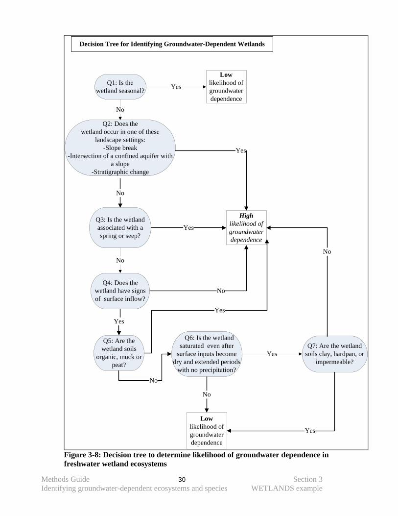
3.3.2.2.A. Wetland decision tree: Below is a decision tree of field indicators to evaluate the importance of groundwater to
freshwater wetlands (Figure 3-8). In this, a series of sequential questions are asked in order to provide an initial assessment of how important groundwater is likely to be as a source of water to a wetland. Many of the indicators are based on the hydrogeologic setting of the wetland, therefore it is important to have a good understanding of the location and position of the wetland in the landscape.
Methods Guide 30 Section 3 Identifying groundwater-dependent ecosystems and species WETLANDS example
Highlikelihood of groundwater dependence
Yes
Yes
No
No
Yes
No
Low likelihood of groundwater dependence
Decision Tree for Identifying Groundwater-Dependent Wetlands
Q2: Does the wetland occur in one of these
landscape settings:-Slope break
-Intersection of a confined aquifer with a slope
-Stratigraphic change
Q4: Does the wetland have signs of surface inflow?
Q6: Is the wetland saturated even after
surface inputs become dry and extended periods
with no precipitation?
Q3: Is the wetland associated with a spring or seep?
No
Q1: Is the wetland seasonal?
No
Lowlikelihood of groundwater dependence
Yes
Q7: Are the wetland soils clay, hardpan, or
impermeable?Yes
Yes
No
Q5: Are the wetland soils
organic, muck or peat?
Yes
No
Figure 3-8: Decision tree to determine likelihood of groundwater dependence in freshwater wetland ecosystems
Methods Guide 31 Section 3 Identifying groundwater-dependent ecosystems and species WETLANDS example
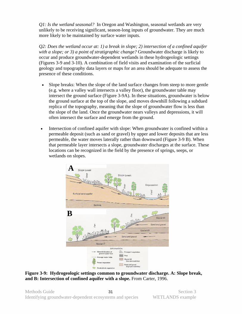
Q1: Is the wetland seasonal? In Oregon and Washington, seasonal wetlands are very unlikely to be receiving significant, season-long inputs of groundwater. They are much more likely to be maintained by surface water inputs. Q2: Does the wetland occur at: 1) a break in slope; 2) intersection of a confined aquifer with a slope; or 3) a point of stratigraphic change? Groundwater discharge is likely to occur and produce groundwater-dependent wetlands in these hydrogeologic settings (Figures 3-9 and 3-10). A combination of field visits and examination of the surficial geology and topography data layers or maps for an area should be adequate to assess the presence of these conditions.
• Slope breaks: When the slope of the land surface changes from steep to more gentle
(e.g. where a valley wall intersects a valley floor), the groundwater table may intersect the ground surface (Figure 3-9A). In these situations, groundwater is below the ground surface at the top of the slope, and moves downhill following a subdued replica of the topography, meaning that the slope of groundwater flow is less than the slope of the land. Once the groundwater nears valleys and depressions, it will often intersect the surface and emerge from the ground.
• Intersection of confined aquifer with slope: When groundwater is confined within a
permeable deposit (such as sand or gravel) by upper and lower deposits that are less permeable, the water moves laterally rather than downward (Figure 3-9 B). When that permeable layer intersects a slope, groundwater discharges at the surface. These locations can be recognized in the field by the presence of springs, seeps, or wetlands on slopes.
Figure 3-9: Hydrogeologic settings common to groundwater discharge. A: Slope break, and B: Intersection of confined aquifer with a slope. From Carter, 1996.
A
B
Methods Guide 32 Section 3 Identifying groundwater-dependent ecosystems and species WETLANDS example
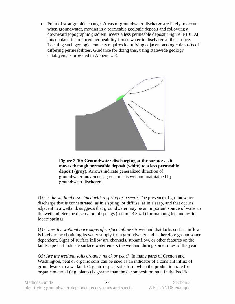
• Point of stratigraphic change: Areas of groundwater discharge are likely to occur when groundwater, moving in a permeable geologic deposit and following a downward topographic gradient, meets a less permeable deposit (Figure 3-10). At this contact, the reduced permeability forces water to discharge at the surface. Locating such geologic contacts requires identifying adjacent geologic deposits of differing permeabilities. Guidance for doing this, using statewide geology datalayers, is provided in Appendix E.
Figure 3-10: Groundwater discharging at the surface as it moves through permeable deposit (white) to a less permeable deposit (gray). Arrows indicate generalized direction of groundwater movement; green area is wetland maintained by groundwater discharge.
Q3: Is the wetland associated with a spring or a seep? The presence of groundwater discharge that is concentrated, as in a spring, or diffuse, as in a seep, and that occurs adjacent to a wetland, suggests that groundwater may be an important source of water to the wetland. See the discussion of springs (section 3.3.4.1) for mapping techniques to locate springs.
Q4: Does the wetland have signs of surface inflow? A wetland that lacks surface inflow is likely to be obtaining its water supply from groundwater and is therefore groundwater dependent. Signs of surface inflow are channels, streamflow, or other features on the landscape that indicate surface water enters the wetland during some times of the year.
Q5: Are the wetland soils organic, muck or peat? In many parts of Oregon and Washington, peat or organic soils can be used as an indicator of a constant influx of groundwater to a wetland. Organic or peat soils form when the production rate for organic material (e.g. plants) is greater than the decomposition rate. In the Pacific
Methods Guide 33 Section 3 Identifying groundwater-dependent ecosystems and species WETLANDS example
Northwest, low decomposition rates often occur under saturated conditions created when there is a steady influx of groundwater; in some cases, such as on the coast, this condition is not related to groundwater inputs as it occurs when the precipitation rate exceeds the evapotranspiration rate Peat soils can be identified either in the field or with the use of the soil survey maps. In the field, peat soils usually are saturated and contain partially decomposed organic material such as pieces of plant leaves, stems, or roots. In soil surveys, the order Histosol or the subgroup histic are generally mucky or peat soils. One caution should be raised with this decision tree question. At times, fens, which are groundwater-fed ecosystems, may be mistaken for bogs, which are fed by precipitation but sometimes similar to fens in terms of species composition and water chemistry. For example, fens that have low concentrations of base cationsa can be mistaken for bogs. In addition, there are many examples of wetlands with peat soils whose names include the word ‘bog’, but which are actually fens and do depend upon groundwater. It can be difficult without detailed field study of hydrology and soil and water chemistry to separate bogs from some types of fens. The easiest way to assess the likelihood that a peatland is a fen is by examining the regional topography. Fens tend to form in landscapes with topographic gradients that favor local and regional groundwater flow paths like the ones described in the hydrogeologic setting discussion above. In contrast, bogs tend to develop in very flat landscapes such as the central states and provinces of North America and lowlands in the arctic. In a more unusual case, bogs can form on the tops of volcanoes and other mountains where there is no possibility of groundwater supply. Particular areas where distinguishing fens from bogs is an issue are Puget Sound Lowlands, the Oregon and Washington coasts and some montane areas along the Canadian border. Q6: Is the wetland saturated even after surface water inputs have dried up and after extended periods with no precipitation? If a wetland remains wet (such as with saturated soils) throughout the season, even after surface water and precipitation inputs have ceased, groundwater may be maintaining the hydrologic regime. If the surface inputs do not dry out, answer ‘no’ to this question as groundwater is likely to be less important than surface water in maintaining this wetland. Occasionally, in cool, wet coastal areas of Washington and Oregon, surface runoff exceeds evaporation, and wetlands can remain wet throughout the season even though groundwater is not a significant component of the water budget. These systems would not be groundwater dependent.
Q7: Are the wetland soils clay, hardpan, or otherwise impermeable? In the eastern portion of Washington and Oregon, some permanent wetlands that lack distinct surface water inflows are ‘perched’ on hardpan soils and thus are isolated from groundwater. The aquitard created by the soils prevents groundwater from reaching the wetlands. The source of water for these wetlands can be either precipitation or diffuse surface water.
a Examples of base cations are Ca2+, Mg2+, and K+. Fens with low concentrations of base cations are termed ‘poor fens’.
Methods Guide 34 Section 3 Identifying groundwater-dependent ecosystems and species WETLANDS example
3.3.2.2.B. Water chemistry: Electrical conductivity (EC) can be used as a rough indicator of the sources of water to a
wetland. Freshwater wetlands receive water from a combination of sources (precipitation, surface water, and/or groundwater). If the EC is known for both the freshwater ecosystem and the different water sources, the wetland water EC can be used to deduce the relative contribution of the possible sourcesb.
Electrical conductivity is a measure of the dissolved ions in solution, which come from the soils or bedrock through which the water travels, as well as from CO2 which dissolves in precipitation as it falls to the ground. EC is measured in units of micro-Siemens per cm, or µS/cm.
In general, the longer the water spends traveling over a substrate, the higher the concentration of dissolved ions. For example, whereas precipitation usually has an EC less than 70 µS/cm, fens on highly insoluble substrate have EC values less than 100µS/cmc and those on more soluble substrates can have EC values ranging from 400-1000 µS/cmd (Aldous, unpublished data). Surface water-fed wetlands have a large range in EC values, depending on local hydrologic conditions and soils. For example, some floodplain wetlands can have EC values more than 1000 µS/cm, if the water has a lot of suspended sediment. Slow-moving surface water without suspended sediments can have much lower EC values, for example 200µS/cm (Aldous, unpublished data).
These general EC values can be used to indicate whether groundwater is likely to be an important source of water to a particular wetland. As an example, if a non-floodplain wetland has an EC value of 600 µS/cm, then groundwater probably acts as a significant source of water. Furthermore, it is likely that this groundwater flows through a fairly soluble geologic deposit. Note that it is important that EC measurements are not made immediately after a rain event, when all water will reflect the recent precipitation signal.
Not all groundwater is high in dissolved ions. Groundwater EC is influenced by: • Chemical composition of infiltrating water – This is determined by the chemical
composition of precipitation, accumulated salts in the soil that dissolve as water moves from the surface to the water table, and soil weathering
• Solubility of subsurface rocks – Very soluble rock types include halite, gypsum, and carbonates; less soluble rocks include granite and basalts.
• The residence time of groundwater (how long it takes to move from recharge to discharge areas) – Slow-moving groundwater has longer to dissolve ions in rocks, and thus usually has higher concentrations of dissolved solids.
Further information on measuring and interpreting EC data are discussed in Appendix D. Given the number of other factors that can cause variability in water chemistry, it is best to have any analysis reviewed by someone familiar with water chemistry, and to use these data in conjunction with other evidence.
b This concept is referred to as a simple mixing model. c These are often termed ‘poor’ fens. Examples of base cations are Ca2+, Mg2+, and K+. d These are termed ‘medium’ or ‘rich’ fens depending upon the concentration of the dissolved base cations.
Methods Guide 35 Section 3 Identifying groundwater-dependent ecosystems and species WETLANDS example
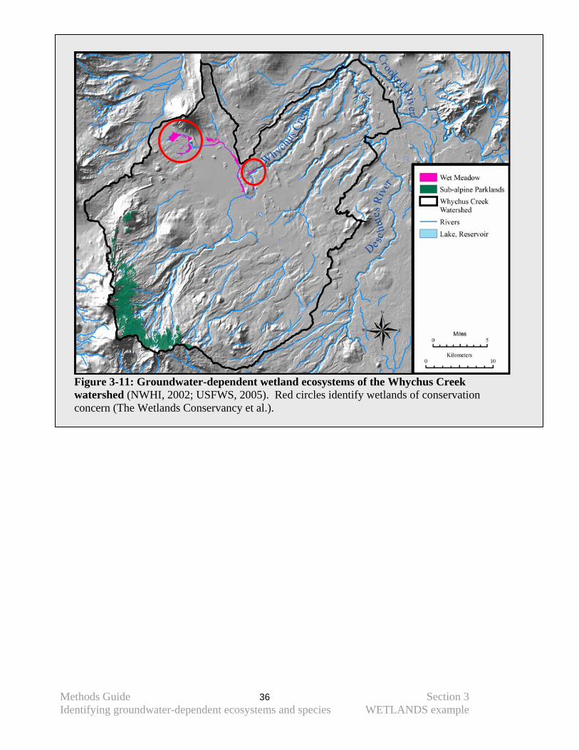
Example: Identifying groundwater-dependent wetland ecosystems: Whychus Creek drainage i. Identifying and mapping wetland ecosystems: Existing wetlands were identified using the National Wetland Inventory data, which were available for part of this watershed. In addition, occurrences of two wetland habitat types, subalpine parklands and wet meadows, were mapped using the database produced by the Northwest Habitat Institute’s Interactive Biodiversity Information System (IBIS) (available at http://www.nwhi.org/index/ibis ). Historic, or potential, wetlands were mapped using the hydric soils data and local wetland assessments. SSURGO data (county by county NRCS soil survey data) for all of this particular area were unavailable digitally so the STATSGO database was used to locate areas with hydric soils. However, as we identified very few areas with hydric soils, this search produced no new potential wetlands. Additional wetlands were added from The Deschutes Wetland Atlas (available at http://www.wetlandsconservancy.org/pdfs/DeschutesWIA.pdf). This product, developed by the Deschutes River Conservancy through a series of GIS analyses, added the Black Butte Ranch and Camp Polk wetlands, which are both wet meadow communities (The Wetlands Conservancy et al.).
All of the wetlands identified using these additional data sources were included in the wetland analysis, except for riparian wetlands which were included under river ecosystems. The wetlands fell into two categories: subalpine parkland and wet meadow (Figure 3-11). The Wetlands Conservancy identified a subset of the wet meadow sites as areas of conservation concern (The Wetlands Conservancy et al.), so these became the areas of focus for this assessment (red circles on Figure 3-11).
Methods Guide 36 Section 3 Identifying groundwater-dependent ecosystems and species WETLANDS example
Figure 3-11: Groundwater-dependent wetland ecosystems of the Whychus Creek watershed (NWHI, 2002; USFWS, 2005). Red circles identify wetlands of conservation concern (The Wetlands Conservancy et al.).
Methods Guide 37 Section 3 Identifying groundwater-dependent ecosystems and species WETLANDS example
ii. Evaluating the importance of groundwater to wetland ecosystems:
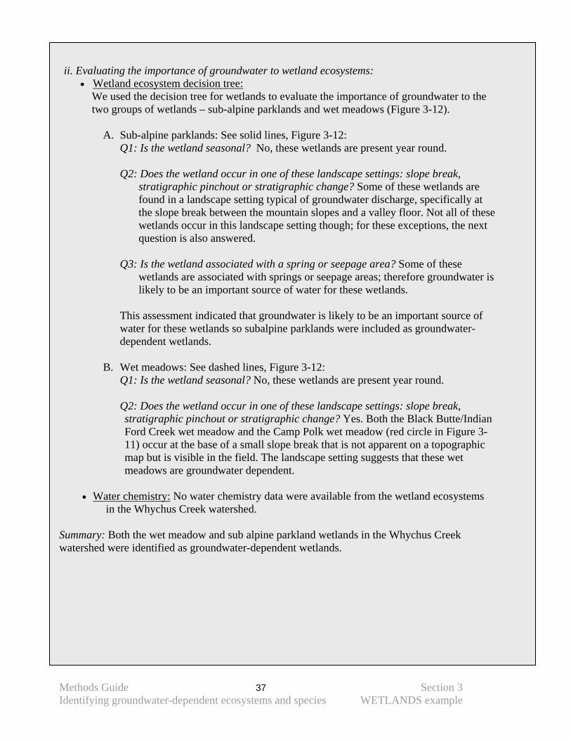
• Wetland ecosystem decision tree: We used the decision tree for wetlands to evaluate the importance of groundwater to the two groups of wetlands – sub-alpine parklands and wet meadows (Figure 3-12).
A. Sub-alpine parklands: See solid lines, Figure 3-12: Q1: Is the wetland seasonal? No, these wetlands are present year round. Q2: Does the wetland occur in one of these landscape settings: slope break,
stratigraphic pinchout or stratigraphic change? Some of these wetlands are found in a landscape setting typical of groundwater discharge, specifically at the slope break between the mountain slopes and a valley floor. Not all of these wetlands occur in this landscape setting though; for these exceptions, the next question is also answered.
Q3: Is the wetland associated with a spring or seepage area? Some of these
wetlands are associated with springs or seepage areas; therefore groundwater is likely to be an important source of water for these wetlands.
This assessment indicated that groundwater is likely to be an important source of water for these wetlands so subalpine parklands were included as groundwater-dependent wetlands.
B. Wet meadows: See dashed lines, Figure 3-12: Q1: Is the wetland seasonal? No, these wetlands are present year round. Q2: Does the wetland occur in one of these landscape settings: slope break, stratigraphic pinchout or stratigraphic change? Yes. Both the Black Butte/Indian Ford Creek wet meadow and the Camp Polk wet meadow (red circle in Figure 3-11) occur at the base of a small slope break that is not apparent on a topographic map but is visible in the field. The landscape setting suggests that these wet meadows are groundwater dependent.
• Water chemistry: No water chemistry data were available from the wetland ecosystems
in the Whychus Creek watershed. Summary: Both the wet meadow and sub alpine parkland wetlands in the Whychus Creek watershed were identified as groundwater-dependent wetlands.
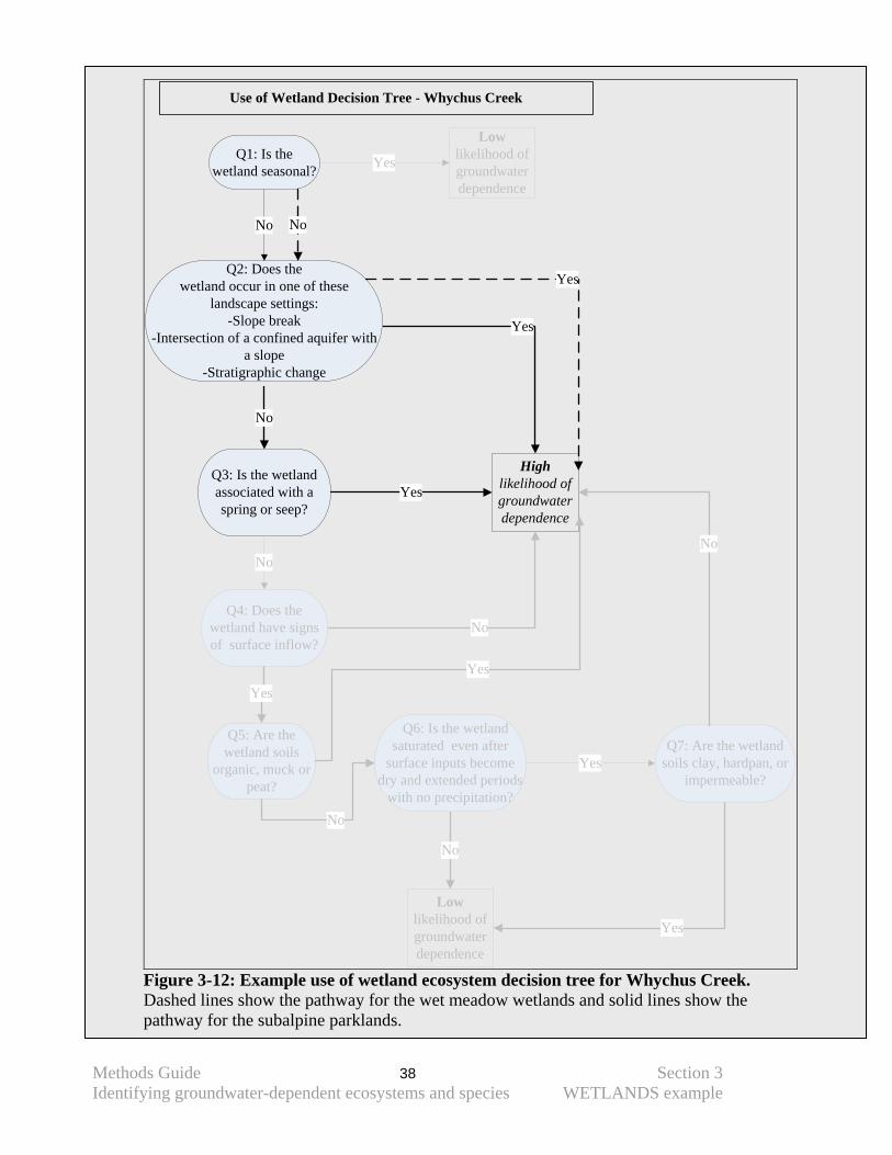
Methods Guide 38 Section 3 Identifying groundwater-dependent ecosystems and species WETLANDS example
High likelihood of groundwater dependence
Yes
Yes
No
No
Yes
No
Lowlikelihood of groundwater dependence
Use of Wetland Decision Tree - Whychus Creek
Q2: Does the wetland occur in one of these
landscape settings:-Slope break
-Intersection of a confined aquifer with a slope
-Stratigraphic change
Q4: Does the wetland have signs of surface inflow?
Q6: Is the wetland saturated even after
surface inputs become dry and extended periods
with no precipitation?
Q3: Is the wetland associated with a spring or seep?
No
Q1: Is the wetland seasonal?
No
Lowlikelihood of groundwater dependence
Yes
Q7: Are the wetland soils clay, hardpan, or
impermeable?Yes
Yes
No
Q5: Are the wetland soils
organic, muck or peat?
Yes
No
Yes
No
Figure 3-12: Example use of wetland ecosystem decision tree for Whychus Creek. Dashed lines show the pathway for the wet meadow wetlands and solid lines show the pathway for the subalpine parklands.
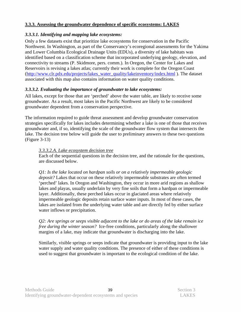
Methods Guide 39 Section 3 Identifying groundwater-dependent ecosystems and species LAKES
3.3.3. Assessing the groundwater dependence of specific ecosystems: LAKES
3.3.3.1. Identifying and mapping lake ecosystems: Only a few datasets exist that prioritize lake ecosystems for conservation in the Pacific Northwest. In Washington, as part of the Conservancy’s ecoregional assessments for the Yakima and Lower Columbia Ecological Drainage Units (EDUs), a diversity of lake habitats was identified based on a classification scheme that incorporated underlying geology, elevation, and connectivity to streams (P. Skidmore, pers. comm.). In Oregon, the Center for Lakes and Reservoirs is revising a lakes atlas; currently their work is complete for the Oregon Coast (http://www.clr.pdx.edu/projects/lakes_water_quality/lakeinventory/index.html ). The dataset associated with this map also contains information on water quality conditions.
3.3.3.2. Evaluating the importance of groundwater to lake ecosystems: All lakes, except for those that are ‘perched’ above the water table, are likely to receive some groundwater. As a result, most lakes in the Pacific Northwest are likely to be considered groundwater dependent from a conservation perspective. The information required to guide threat assessment and develop groundwater conservation strategies specifically for lakes includes determining whether a lake is one of those that receives groundwater and, if so, identifying the scale of the groundwater flow system that intersects the lake. The decision tree below will guide the user to preliminary answers to these two questions (Figure 3-13)
3.3.3.2.A. Lake ecosystem decision tree Each of the sequential questions in the decision tree, and the rationale for the questions, are discussed below. Q1: Is the lake located on hardpan soils or on a relatively impermeable geologic deposit? Lakes that occur on these relatively impermeable substrates are often termed ‘perched’ lakes. In Oregon and Washington, they occur in more arid regions as shallow lakes and playas, usually underlain by very fine soils that form a hardpan or impermeable layer. Additionally, these perched lakes occur in glaciated areas where relatively impermeable geologic deposits retain surface water inputs. In most of these cases, the lakes are isolated from the underlying water table and are directly fed by either surface water inflows or precipitation. Q2: Are springs or seeps visible adjacent to the lake or do areas of the lake remain ice free during the winter season? Ice-free conditions, particularly along the shallower margins of a lake, may indicate that groundwater is discharging into the lake. Similarly, visible springs or seeps indicate that groundwater is providing input to the lake water supply and water quality conditions. The presence of either of these conditions is used to suggest that groundwater is important to the ecological condition of the lake.
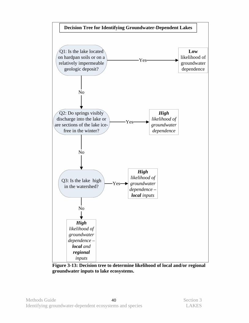
Methods Guide 40 Section 3 Identifying groundwater-dependent ecosystems and species LAKES
Yes
Low likelihood of groundwater dependence
Yes
No
No
Decision Tree for Identifying Groundwater-Dependent Lakes
Q1: Is the lake located on hardpan soils or on a relatively impermeable
geologic deposit?
Q3: Is the lake high in the watershed?
Highlikelihood of groundwater dependence
Q2: Do springs visibly discharge into the lake or
are sections of the lake ice-free in the winter?
No
Yes
Highlikelihood of groundwater dependence –local inputs
Highlikelihood of groundwater dependence –
local and regional inputs
Figure 3-13: Decision tree to determine likelihood of local and/or regional groundwater inputs to lake ecosystems.
Methods Guide 41 Section 3 Identifying groundwater-dependent ecosystems and species LAKES
Q3: Is the lake in the upper portion of the watershed? Lakes that are high in a watershed usually only receive local groundwater inputs whereas lakes lower in the watershed can receive both local and regional inputs. As discussed in Section 2, Groundwater Basics, groundwater flow systems of different scales can overlie each other. Often, within a watershed that is dominated by permeable deposits, locally recharged groundwater moves into a lake on the upgradient side and then moves out of the lake, back into the ground, on the down gradient side of the lake. Some of the recharge that occurs on this downgradient side may move deeper into the subsurface, recharging the regional groundwater flow system (see Figure 2-3). As a result, the area of the landscape that contributes groundwater to a lake can be a function of the position of the lake within a watershed.
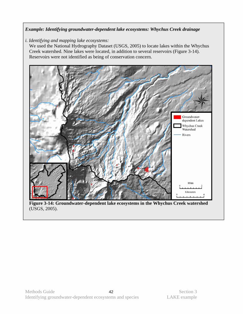
Methods Guide 42 Section 3 Identifying groundwater-dependent ecosystems and species LAKE example
Example: Identifying groundwater-dependent lake ecosystems: Whychus Creek drainage i. Identifying and mapping lake ecosystems:
We used the National Hydrography Dataset (USGS, 2005) to locate lakes within the Whychus Creek watershed. Nine lakes were located, in addition to several reservoirs (Figure 3-14). Reservoirs were not identified as being of conservation concern.
Figure 3-14: Groundwater-dependent lake ecosystems in the Whychus Creek watershed (USGS, 2005).

Methods Guide 43 Section 3 Identifying groundwater-dependent ecosystems and species LAKE example
ii. Evaluating the importance of groundwater on lake ecosystems:
We used the decision tree to evaluate the importance of groundwater to the lake ecosystems (Figure 3-15):
Q1: Is the lake located on hardpan soils or a relatively impermeable geologic deposit? No, these lakes are all located on relatively permeable geologic deposits.
Q2:Do springs or seeps visibly discharge into the lake or are portions of the lake ice-free during the winter? No, not that we know of. Q3: Is the lake high in the watershed? Yes, all of these lakes are in the upper portion of the watershed suggesting that the source of groundwater input is fairly local and from the immediate surface watershed.
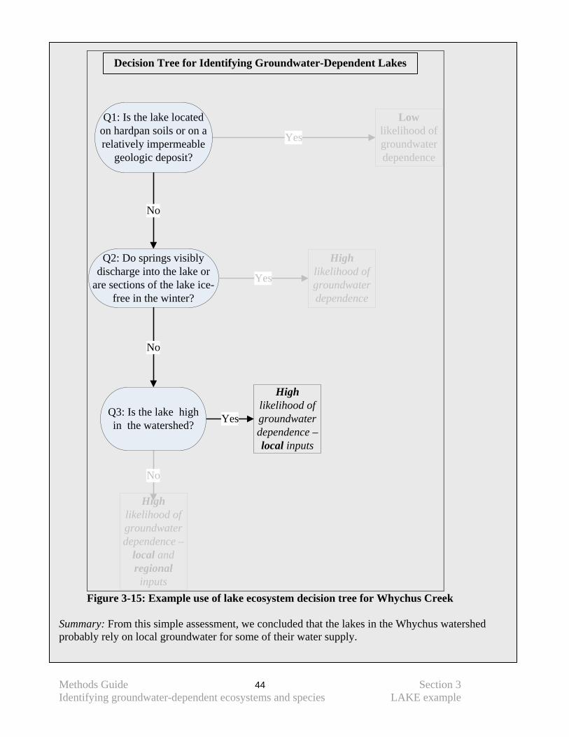
Methods Guide 44 Section 3 Identifying groundwater-dependent ecosystems and species LAKE example
Yes
Yes
No
No
Decision Tree for Identifying Groundwater-Dependent Lakes
Q1: Is the lake located on hardpan soils or on a relatively impermeable
geologic deposit?
Q3: Is the lake high in the watershed?
Q2: Do springs visibly discharge into the lake or
are sections of the lake ice-free in the winter?
No
Yes
Low likelihood of groundwater dependence
Highlikelihood of groundwater dependence
Highlikelihood of groundwater dependence –local inputs
Highlikelihood of groundwater dependence –
local and regional inputs
Figure 3-15: Example use of lake ecosystem decision tree for Whychus Creek
Summary: From this simple assessment, we concluded that the lakes in the Whychus watershed probably rely on local groundwater for some of their water supply.
Methods Guide 45 Section 3 Identifying groundwater-dependent ecosystems and species SPRINGS
3.3.4. Assessing the groundwater dependence of specific ecosystems: SPRINGS
3.3.4.1. Identifying and mapping springs: Little data exist that identify springs of conservation concern, although rare species associated with springs are often tracked by the Natural Heritage Program. This absence of information is partially due to the lack of spatial information on spring locations across large geographic areas. In the Conservancy’s ecoregional assessments, springs are often embedded in larger ecosystems and not identified individually. Several approaches can be used to locate springs more completely.
• Datasets and Maps: Three datasets may be useful for identifying location of springs in the Pacific Northwest:
a. National Hydrography Data: This dataset is produced by USGS and contains some spring locations. Use the DESIG field to identify ‘springs’.
b. Pacific Northwest Hydrography Framework Clearinghouse (http://hydro.reo.gov/index.html): The ‘water points’ dataset being developed by this group contains springs in Oregon. It is not complete but provides an additional set of springs to those located on the NHD dataset.
c. Additional springs can be located from maps such as the Gazeteer, USGS topo maps or the Geographic Names Information System (USGS, 1996).
• Aerial photos: The National Agricultural Imagery Program took 1 and 2 m digital aerial
photos in 2006 for Washington and 2005 for Oregon (http://datagateway.nrcs.usda.gov). Springs can often be identified by green vegetation, particularly in arid regions, later in the summer season.
• Ice free conditions: Springs are often located where ice-free conditions exist during the
ice formation period (Tom Winter, pers. comm.) or warmer water temperature exists during the winter season.
• Hydrogeologic setting: Springs tend to occur in two types of hydrogeologic settings -
a. Where surface topography causes the water table to intersect the land slope Two examples of this type of setting are shown in A and B of Figure 3-16. This setting can often be predicted or identified on the landscape using the surface topography as a guide as described for wetlands in Figures 3-9A and B. In general, springs of this nature tend to be supported by more local groundwater flow systems and thus are at risk from activities that threaten the shallow water table. b. Where subsurface geologic structure forces groundwater to emerge at the surface These spring locations are not defined by the surface topography but rather by the subsurface geologic conditions. Examples of these situations are shown in C-F of Figure 3-16. Identifying these conditions from the field is often difficult. Often these springs are supplied by deeper, more regional groundwater flows and are therefore at risk from activities that threaten the deeper water flow system.
• Remote sensing: Additional indications of spring locations can be obtained by identifying
areas of cold water from Forward Looking Infrared (FLIR) data. These data are collected

Methods Guide 46 Section 3 Identifying groundwater-dependent ecosystems and species SPRINGS
by airborne sensors that assess water temperature. Colder areas are likely points of groundwater discharge, either as seepage or a spring. More information on this technique, its data requirements and the type of information it generates are given in Appendix D.
3.3.4.2. Evaluating the importance of groundwater to spring ecosystems: All spring ecosystems depend upon groundwater by definition.
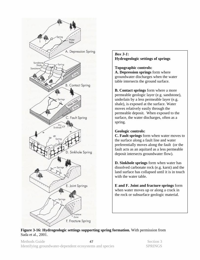
Methods Guide 47 Section 3 Identifying groundwater-dependent ecosystems and species SPRINGS
Figure 3-16: Hydrogeologic settings supporting spring formation. With permission from Sada et al., 2001.
Box 3-1: Hydrogeologic settings of springs Topographic controls: A. Depression springs form where groundwater discharges when the water table intersects the ground surface. B. Contact springs form where a more permeable geologic layer (e.g. sandstone), underlain by a less permeable layer (e.g. shale), is exposed at the surface. Water moves relatively easily through the permeable deposit. When exposed to the surface, the water discharges, often as a spring. Geologic controls: C. Fault springs form when water moves to the surface along a fault line and water preferentially moves along the fault (or the fault acts as an aquitard as a less permeable deposit intersects groundwater flow). D. Sinkhole springs form when water has dissolved carbonate rock (e.g. karst) and the land surface has collapsed until it is in touch with the water table. E and F. Joint and fracture springs form when water moves up or along a crack in the rock or subsurface geologic material.
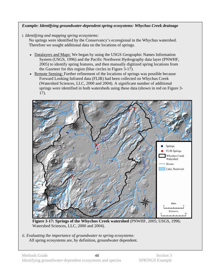
Methods Guide 48 Section 3 Identifying groundwater-dependent ecosystems and species SPRINGS Example
Example: Identifying groundwater-dependent spring ecosystems: Whychus Creek drainage i. Identifying and mapping spring ecosystems:
No springs were identified by the Conservancy’s ecoregional in the Whychus watershed. Therefore we sought additional data on the locations of springs.
• Datalayers and Maps: We began by using the USGS Geographic Names Information
System (USGS, 1996) and the Pacific Northwest Hydrography data layer (PNWHF, 2005) to identify spring features, and then manually digitized spring locations from the Gazeteer for this region (blue circles in Figure 3-17).
• Remote Sensing: Further refinement of the locations of springs was possible because Forward Looking Infrared data (FLIR) had been collected on Whychus Creek (Watershed Sciences, LLC, 2000 and 2004). A significant number of additional springs were identified in both watersheds using these data (shown in red on Figure 3-17).
Figure 3-17: Springs of the Whychus Creek watershed (PNWHF, 2005; USGS, 1996; Watershed Sciences, LLC, 2000 and 2004).
ii. Evaluating the importance of groundwater to spring ecosystems: All spring ecosystems are, by definition, groundwater dependent.
Methods Guide 49 Section 3 Identifying groundwater-dependent ecosystems and species PHREATOPHYTES
3.3.5. Assessing the groundwater dependence of specific ecosystems: PHREATOPHYTIC ECOSYSTEMS:
3.3.5.1. Identifying and mapping phreatophytic ecosystems: Species of phreatophytic vegetation obtain water from groundwater that is near the surface – termed ‘shallow groundwater’. These species are characterized by deep roots that extract water from the capillary fringe – the subsurface area just above the water table that is not completely saturated. Even though the groundwater may never be visible at the ground surface, as it is in a wetland or spring, phreatophytic ecosystems can be groundwater dependent (Naumberg et al., 2005). Obligate phreatophytes occur only in settings where the water table is near the surface and can be accessed by their deep roots (Naiman et al., 2006); all of these species are groundwater dependent. Facultative phreatophytes can use groundwater if it is available but can also occur in upland settings where groundwater is not available (Naiman et al., 2006). The dependence of these species on groundwater is a function of the hydrogeologic setting of the ecosystem, which governs whether a shallow water table exists that the species can use. The use of groundwater may not be year round. In these instances, other water sources are used in the wet season but groundwater is used in the dry season (Froend and Loomes, 2004). Phreatophytes can occur in both upland and riparian settings and in both humid and arid regions. There are examples of streamside species (such as Salix goodingii) that grow adjacent to a stream, but have deep roots and utilize groundwater instead of streamwater (Dawson and Ehleringer, 1991; Busch et al., 1992). The identification of phreatophytic ecosystems can be challenging because there is no comprehensive list of phreatophytes for the Pacific Northwest. Below are some guidelines for deciding if a species or ecosystem is phreatophytic (Le Maitre et al., 1999; Froend and Loomis, 2004):
• A species is known to depend upon shallow groundwater: Some species which have been documented as phreatophytes are listed in Table 3-1. Individual ecosystems and their dependence on shallow groundwater can sometimes be found on the NatureServe Explorer website (http://www.natureserve.org/). Additionally, expert knowledge will be useful in identifying phreatophytic species.
Table 3-1 Documented phreatophytes that occur in the Pacific Northwest Species Common Name Reference
Salix gooddingii Gooding willow Busch et al., 1992 Populus fremontii Cottonwood Busch et al., 1992 Prosopis velutina Mesquite Hultine et al., 2004 Chrysothamnus nauseosus Rabbitbrush Hacke et al., 2000 Pseudotsuga menziesii Douglas Fir Brooks et al., 2002
Phreatophytic vegetation: Vegetation with deep roots that extend near the saturated zone (or water table) and receive water from the capillary fringe just above the water table.
Methods Guide 50 Section 3 Identifying groundwater-dependent ecosystems and species PHREATOPHYTES
• A species is known to have roots extending over a meter in depth. Root depth of some more common species can be found in the literature; two review articles that may help are Jackson et al. (1996) and Stone and Kalisz (1991).
• The community occurs in areas where the water table is known to be near the surface. • In arid regions, the herbaceous or shrub vegetation is green or has high leaf area late in
the season; this contrasts with other dry areas in the same watershed that do not access groundwater.
Additionally, stable isotope analysis can be used to identify whether groundwater is supplying water to vegetation (Froend and Loomis, 2004). Details of this analysis are provided in Appendix D.
3.3.5.2. Evaluating the importance of groundwater to phreatophytic ecosystems: All phreatophytic ecosystems depend upon groundwater.
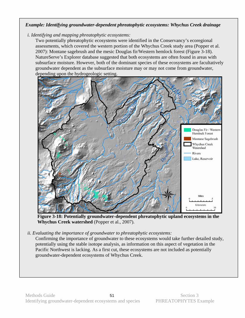
Methods Guide 51 Section 3 Identifying groundwater-dependent ecosystems and species PHREATOPHYTES Example
Example: Identifying groundwater-dependent phreatophytic ecosystems: Whychus Creek drainage i. Identifying and mapping phreatophytic ecosystems:
Two potentially phreatophytic ecosystems were identified in the Conservancy’s ecoregional assessments, which covered the western portion of the Whychus Creek study area (Popper et al. 2007): Montane sagebrush and the mesic Douglas fir/Western hemlock forest (Figure 3-18). NatureServe’s Explorer database suggested that both ecosystems are often found in areas with subsurface moisture. However, both of the dominant species of these ecosystems are facultatively groundwater dependent as the subsurface moisture may or may not come from groundwater, depending upon the hydrogeologic setting.
Figure 3-18: Potentially groundwater-dependent phreatophytic upland ecosystems in the Whychus Creek watershed (Popper et al., 2007).
ii. Evaluating the importance of groundwater to phreatophytic ecosystems: Confirming the importance of groundwater to these ecosystems would take further detailed study, potentially using the stable isotope analysis, as information on this aspect of vegetation in the Pacific Northwest is lacking. As a first cut, these ecosystems are not included as potentially groundwater-dependent ecosystems of Whychus Creek.
Methods Guide 52 Section 3 Identifying groundwater-dependent ecosystems and species CAVES
3.3.6. Assessing the groundwater dependence of specific ecosystems: CAVES
3.3.6.1. Identifying and mapping cave ecosystems: Identifying caves of conservation concern requires the use of local maps and geologic information. No readily available map of caves for Oregon or Washington has been located, due to cave protection laws, but the USGS publishes a map of potential bat habitat in the Interior Columbia Basin, which is based upon the likelihood that caves will form in the surficial geologic deposits (http://www.icbemp.gov/spatial/min, scroll down to ‘potential bat habitat’). Additionally, the USGS has developed a datalayer of karst and psuedokarst across the country (http://nationalatlas.gov/atlasftp.html#karst0m, see ‘Karst’, ‘engineering properties’). Neither of these identifies specific caves but rather material from which caves form.
3.3.6.2. Evaluating the importance of groundwater to cave ecosystems: All cave ecosystems depend upon groundwater.
Example: Identifying groundwater-dependent cave ecosystems: Whychus Creek drainage While lava tube caves are found in the watershed, there are no mapped caves in this watershed. This is an area for further refinement.
Methods Guide 53 Section 3 Identifying groundwater-dependent ecosystems and species SPECIES
3.4 Identifying groundwater-dependent species: In addition to the ecosystems discussed above, some individual species may be groundwater dependent. Species can be obligately or facultatively groundwater dependent, depending upon their groundwater requirements. A species is obligately dependent upon groundwater if at some point during its life history or at particular times of the year it:
• requires habitat that is associated with or maintained by groundwater discharge • requires habitat that is associated with or maintained by a shallow water table • requires water chemistry or quality conditions that are provided by or significantly
influenced by groundwater • is currently restricted to locations of groundwater discharge
A species is facultatively dependent upon groundwater if it does not always require groundwater to meet its habitat requirements. In some locations, these species occur in habitats or ecosystems that are maintained by groundwater; however, these same species can also occur in ecosystems that are not maintained by groundwater as long as their habitat requirements are met. Some resources that can identify species of conservation concern are:
• Ecoregional assessments from The Nature Conservancy (http://conserveonline.org/browse_by_category?category=Ecoregional%20Planning )
• US Forest Service Watershed Analysis documents • Natural Heritage databases • Partners in Flight data
Each species of conservation concern will need to be evaluated for its dependence on groundwater. The requirements of individual species may be found in the literature or on the web. We suggest using NatureServe’s Explorer as a starting point for evaluating the likelihood that a particular species depends upon groundwater (http://www.natureserve.org/explorer/). Web searches can also be productive as many states have online encyclopedias or atlases of different species. Local experts on various taxonomic groups can also provide important information about the dependence of particular species on groundwater. All of these resources (and any others that are available) can help to focus the list of species of conservation concern to those that depend upon groundwater.
Methods Guide 54 Section 3 Identifying groundwater-dependent ecosystems and species SPECIES Example
Example: Identifying groundwater-dependent species: Whychus Creek drainage i. Identifying groundwater-dependent species: We used The Nature Conservancy’s ecoregional assessments and a US Forest Service watershed analysis (USFS, 1998) to identify species of conservation concern in the Whychus Creek drainage that are both facultatively and obligately dependent upon groundwater. This list was supplemented and checked with input from local experts (Table 3-2). Bull trout (Popper et al., 2007) and resident redband trout (Riehle and Lovtang, 2000) are salmonids currently present in Whychus Creek (Table 3-2). While other salmonids were found in this watershed historically, Pelton River Dam on the mainstem of the Deschutes River is a migration barrier from the lower Deschutes. There are currently ongoing discussions about providing fish passage around this dam and local experts indicated that two salmonids – spring Chinook and summer steelhead – are also fish of conservation concern that are likely to depend upon groundwater in this area once fish passage is provided. These species were also included in Table 3-2. Many of the species in Table 3-2 are facultatively dependent on groundwater. Using our knowledge of ecosystems in the Whychus drainage that depend on groundwater, we were able to evaluate which species are likely to depend on groundwater in this watershed. For instance, the coastal tailed frog (orange circle, Figure 3-19) requires cold water; in the portion of the Whychus watershed where this frog occurs, cold water is supplied by groundwater discharge, so it is included as a groundwater-dependent species. ii. Mapping groundwater-dependent species We were able to map the known occurrences of most of the groundwater-dependent species in Table 3-2 (Figure 3-19). However, locational data for the Cascades Apatanian Caddisfly (Apatania tavala) were not available. In addition, except for bull trout, only current distributions, not historic or potential distributions, of species are shown in the maps (Figure 3-19).
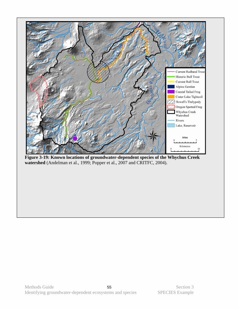
Methods Guide 55 Section 3 Identifying groundwater-dependent ecosystems and species SPECIES Example
Figure 3-19: Known locations of groundwater-dependent species of the Whychus Creek watershed (Andelman et al., 1999; Popper et al., 2007 and CRITFC, 2004).
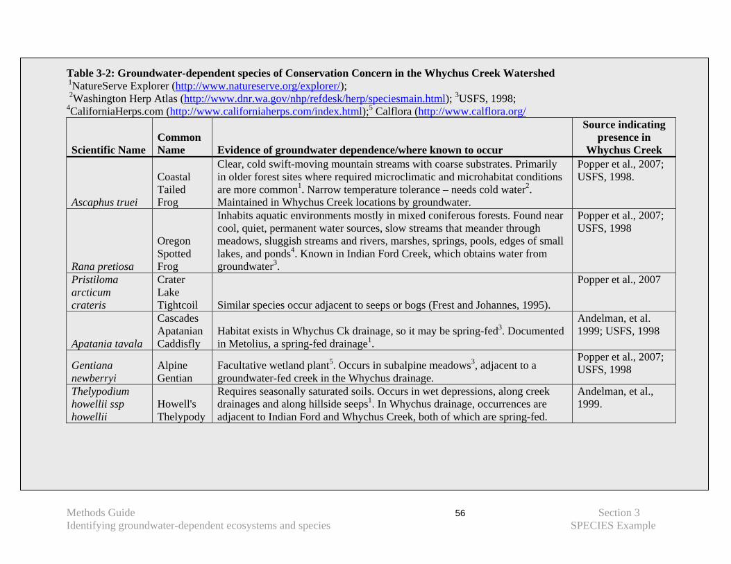
Methods Guide 56 Section 3 Identifying groundwater-dependent ecosystems and species SPECIES Example
Table 3-2: Groundwater-dependent species of Conservation Concern in the Whychus Creek Watershed 1NatureServe Explorer (http://www.natureserve.org/explorer/); 2Washington Herp Atlas (http://www.dnr.wa.gov/nhp/refdesk/herp/speciesmain.html); 3USFS, 1998; 4CaliforniaHerps.com (http://www.californiaherps.com/index.html);5 Calflora (http://www.calflora.org/
Scientific Name Common Name Evidence of groundwater dependence/where known to occur
Source indicating presence in
Whychus Creek
Ascaphus truei
Coastal Tailed Frog
Clear, cold swift-moving mountain streams with coarse substrates. Primarily in older forest sites where required microclimatic and microhabitat conditions are more common1. Narrow temperature tolerance – needs cold water2. Maintained in Whychus Creek locations by groundwater.
Popper et al., 2007; USFS, 1998.
Rana pretiosa
Oregon Spotted Frog
Inhabits aquatic environments mostly in mixed coniferous forests. Found near cool, quiet, permanent water sources, slow streams that meander through meadows, sluggish streams and rivers, marshes, springs, pools, edges of small lakes, and ponds4. Known in Indian Ford Creek, which obtains water from groundwater3.
Popper et al., 2007; USFS, 1998
Pristiloma arcticum crateris
Crater Lake Tightcoil Similar species occur adjacent to seeps or bogs (Frest and Johannes, 1995).
Popper et al., 2007
Apatania tavala
Cascades Apatanian Caddisfly
Habitat exists in Whychus Ck drainage, so it may be spring-fed3. Documented in Metolius, a spring-fed drainage1.
Andelman, et al. 1999; USFS, 1998
Gentiana newberryi
Alpine Gentian
Facultative wetland plant5. Occurs in subalpine meadows3, adjacent to a groundwater-fed creek in the Whychus drainage.
Popper et al., 2007; USFS, 1998
Thelypodium howellii ssp howellii
Howell's Thelypody
Requires seasonally saturated soils. Occurs in wet depressions, along creek drainages and along hillside seeps1. In Whychus drainage, occurrences are adjacent to Indian Ford and Whychus Creek, both of which are spring-fed.
Andelman, et al., 1999.
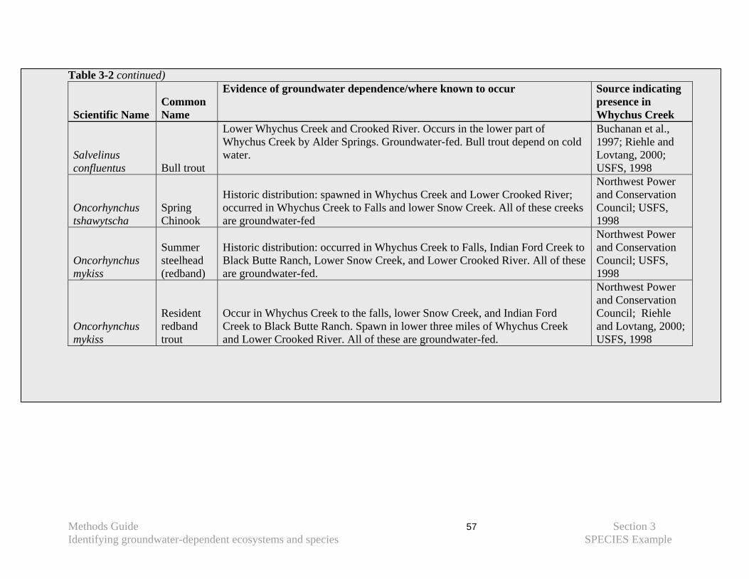
Methods Guide 57 Section 3 Identifying groundwater-dependent ecosystems and species SPECIES Example
Table 3-2 continued) Scientific Name
Common Name
Evidence of groundwater dependence/where known to occur Source indicating presence in Whychus Creek
Salvelinus confluentus Bull trout
Lower Whychus Creek and Crooked River. Occurs in the lower part of Whychus Creek by Alder Springs. Groundwater-fed. Bull trout depend on cold water.
Buchanan et al., 1997; Riehle and Lovtang, 2000; USFS, 1998
Oncorhynchus tshawytscha
Spring Chinook
Historic distribution: spawned in Whychus Creek and Lower Crooked River; occurred in Whychus Creek to Falls and lower Snow Creek. All of these creeks are groundwater-fed
Northwest Power and Conservation Council; USFS, 1998
Oncorhynchus mykiss
Summer steelhead (redband)
Historic distribution: occurred in Whychus Creek to Falls, Indian Ford Creek to Black Butte Ranch, Lower Snow Creek, and Lower Crooked River. All of these are groundwater-fed.
Northwest Power and Conservation Council; USFS, 1998
Oncorhynchus mykiss
Resident redband trout
Occur in Whychus Creek to the falls, lower Snow Creek, and Indian Ford Creek to Black Butte Ranch. Spawn in lower three miles of Whychus Creek and Lower Crooked River. All of these are groundwater-fed.
Northwest Power and Conservation Council; Riehle and Lovtang, 2000; USFS, 1998
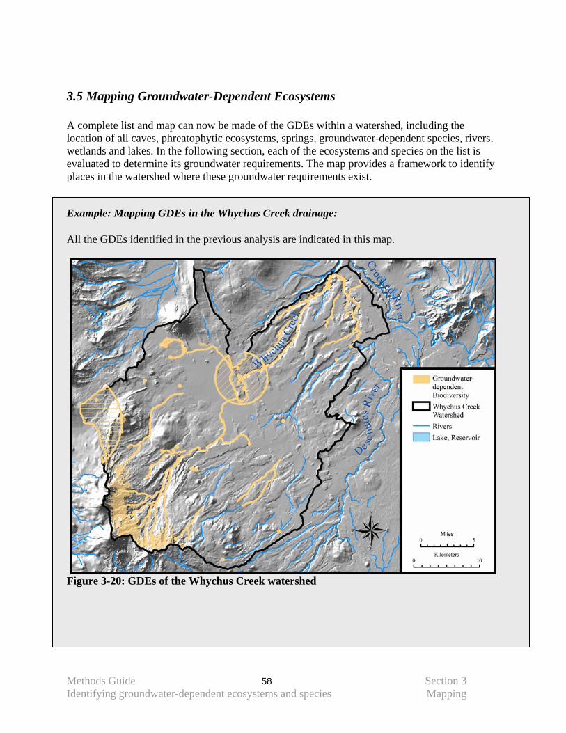
Methods Guide 58 Section 3 Identifying groundwater-dependent ecosystems and species Mapping
3.5 Mapping Groundwater-Dependent Ecosystems A complete list and map can now be made of the GDEs within a watershed, including the location of all caves, phreatophytic ecosystems, springs, groundwater-dependent species, rivers, wetlands and lakes. In the following section, each of the ecosystems and species on the list is evaluated to determine its groundwater requirements. The map provides a framework to identify places in the watershed where these groundwater requirements exist.
Example: Mapping GDEs in the Whychus Creek drainage: All the GDEs identified in the previous analysis are indicated in this map.
Figure 3-20: GDEs of the Whychus Creek watershed
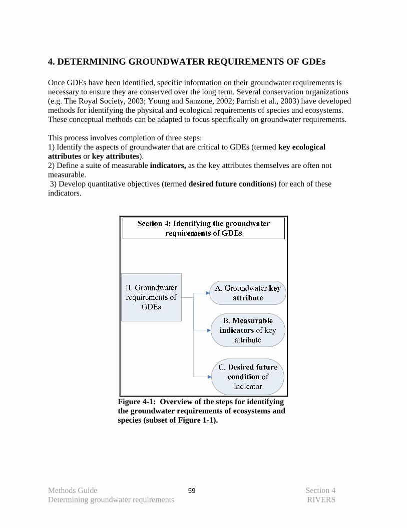
Methods Guide 59 Section 4 Determining groundwater requirements RIVERS
4. DETERMINING GROUNDWATER REQUIREMENTS OF GDEs Once GDEs have been identified, specific information on their groundwater requirements is necessary to ensure they are conserved over the long term. Several conservation organizations (e.g. The Royal Society, 2003; Young and Sanzone, 2002; Parrish et al., 2003) have developed methods for identifying the physical and ecological requirements of species and ecosystems. These conceptual methods can be adapted to focus specifically on groundwater requirements. This process involves completion of three steps: 1) Identify the aspects of groundwater that are critical to GDEs (termed key ecological attributes or key attributes). 2) Define a suite of measurable indicators, as the key attributes themselves are often not measurable. 3) Develop quantitative objectives (termed desired future conditions) for each of these indicators.
Figure 4-1: Overview of the steps for identifying the groundwater requirements of ecosystems and species (subset of Figure 1-1).
Methods Guide 60 Section 4 Determining groundwater requirements RIVERS
Attributes, indicators and desired future conditions are, by their nature, very site-specific; therefore, a comprehensive list for GDEs cannot be developed. As part of this document, we provide example key attributes and indicators for all of the ecosystems discussed previously, except for caves. In Appendix F we provide examples of key attributes and indicators for two species, bull trout and springsnails, and at the end of this section we provide an example of key ecological attributes and indicators for the Whychus Creek watershed.
4.1 Groundwater key attribute Key ecological attributes are those factors that are essential to defining or determining the integrity of a particular GDE. Ecosystems and species can rely on groundwater for three key ecological attributes:
1. An adequate supply of water throughout the year – termed ‘hydrologic regime’ 2. Water of high quality or with a certain chemical composition 3. Water of a specific temperature, either cold or hot.
The importance of each of these attributes varies by GDE. To facilitate conservation planning, the selection of key attributes should focus on the factors that truly define integrity, rather than creating a complete list of important attributes.
4.2 Measurable indicators of key attributes While the attributes that are identified should be key to the integrity of a GDE, the indicators should be measurable and provide usable information about the key attributes. These form the basis of a monitoring program. Indicators should be (Cairns et al., 1993):
Biologically relevant Socially relevant Measurable and interpretable Appropriately precise Anticipatory Cost-effective
In other words an indicator should be relatively easy and inexpensive to measure, should provide information that will directly inform a management response, and should provide early warning of a problem.
4.3 Desired future condition of indicators Articulating a quantifiable desired future condition for each indicator is a critical step in establishing an adaptive management approach to conservation. As indicators are monitored over time, the effectiveness of various strategies can be determined by evaluating the progress made toward achieving the desired future conditions. The desired future conditions should be based upon the best information available. However, because assumptions often are made when developing quantitative objectives, it is critically important that the rationale, logic, and supporting information involved in the decision making be clear and well documented. After several years of monitoring, it may become clear that the objectives were not reasonable or new research may emerge that brings one of the key assumptions into question. With this new information the desired future conditions can be re-evaluated and rewritten.
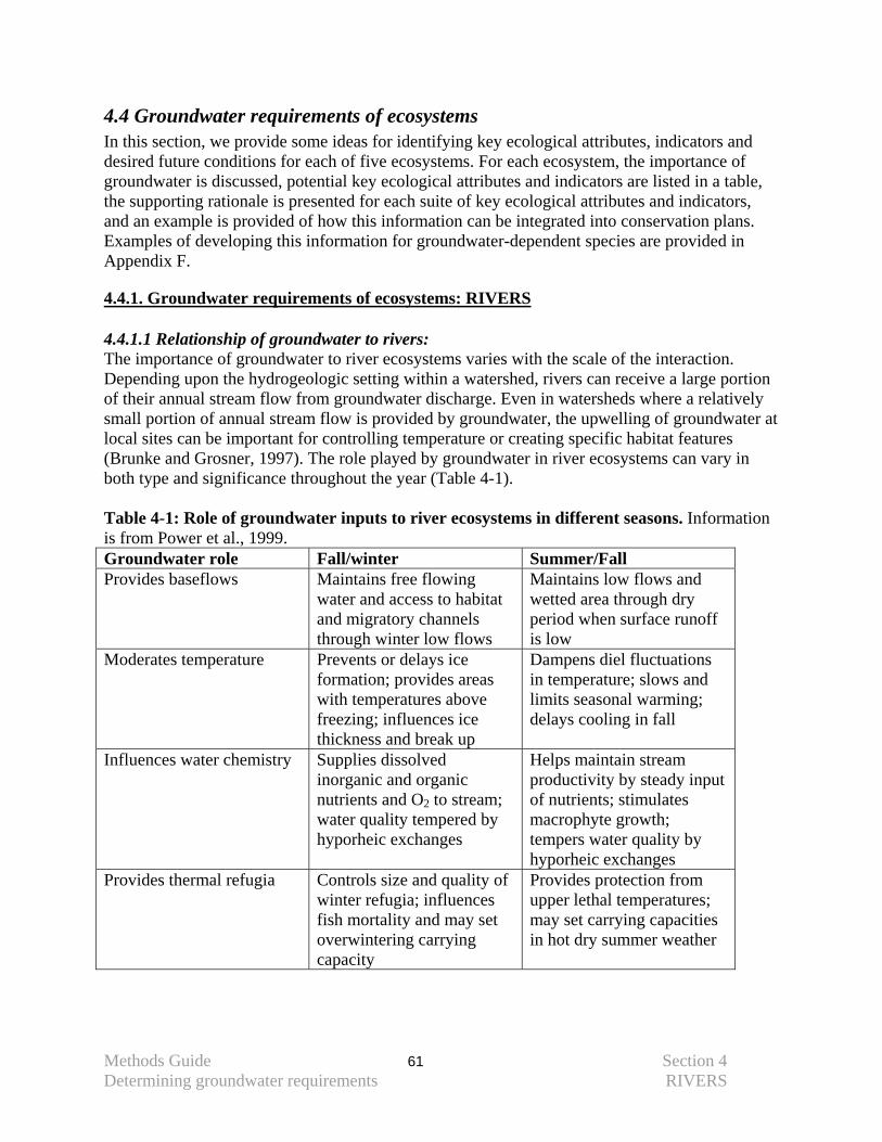
Methods Guide 61 Section 4 Determining groundwater requirements RIVERS
4.4 Groundwater requirements of ecosystems In this section, we provide some ideas for identifying key ecological attributes, indicators and desired future conditions for each of five ecosystems. For each ecosystem, the importance of groundwater is discussed, potential key ecological attributes and indicators are listed in a table, the supporting rationale is presented for each suite of key ecological attributes and indicators, and an example is provided of how this information can be integrated into conservation plans. Examples of developing this information for groundwater-dependent species are provided in Appendix F.
4.4.1. Groundwater requirements of ecosystems: RIVERS 4.4.1.1 Relationship of groundwater to rivers: The importance of groundwater to river ecosystems varies with the scale of the interaction. Depending upon the hydrogeologic setting within a watershed, rivers can receive a large portion of their annual stream flow from groundwater discharge. Even in watersheds where a relatively small portion of annual stream flow is provided by groundwater, the upwelling of groundwater at local sites can be important for controlling temperature or creating specific habitat features (Brunke and Grosner, 1997). The role played by groundwater in river ecosystems can vary in both type and significance throughout the year (Table 4-1). Table 4-1: Role of groundwater inputs to river ecosystems in different seasons. Information is from Power et al., 1999. Groundwater role Fall/winter Summer/Fall Provides baseflows Maintains free flowing
water and access to habitat and migratory channels through winter low flows
Maintains low flows and wetted area through dry period when surface runoff is low
Moderates temperature Prevents or delays ice formation; provides areas with temperatures above freezing; influences ice thickness and break up
Dampens diel fluctuations in temperature; slows and limits seasonal warming; delays cooling in fall
Influences water chemistry Supplies dissolved inorganic and organic nutrients and O2 to stream; water quality tempered by hyporheic exchanges
Helps maintain stream productivity by steady input of nutrients; stimulates macrophyte growth; tempers water quality by hyporheic exchanges
Provides thermal refugia Controls size and quality of winter refugia; influences fish mortality and may set overwintering carrying capacity
Provides protection from upper lethal temperatures; may set carrying capacities in hot dry summer weather
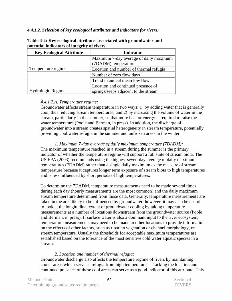
Methods Guide 62 Section 4 Determining groundwater requirements RIVERS
4.4.1.2. Selection of key ecological attributes and indicators for rivers: Table 4-2: Key ecological attributes associated with groundwater and potential indicators of integrity of rivers
Key Ecological Attribute Indicator Maximum 7-day average of daily maximum (7DADM) temperature
Temperature regime Location and number of thermal refugia Number of zero flow days Trend in annual mean low flow
Hydrologic Regime Location and continued presence of springs/seeps adjacent to the stream
4.4.1.2.A. Temperature regime: Groundwater affects stream temperature in two ways: 1) by adding water that is generally cool, thus reducing stream temperatures; and 2) by increasing the volume of water in the stream, particularly in the summer, so that more heat or energy is required to raise the water temperature (Poole and Berman, in press). In addition, the discharge of groundwater into a stream creates spatial heterogeneity in stream temperature, potentially providing cool water refugia in the summer and unfrozen areas in the winter.
1. Maximum 7-day average of daily maximum temperature (7DADM):
The maximum temperature reached in a stream during the summer is the primary indicator of whether the temperature regime will support a full suite of stream biota. The US EPA (2003) recommends using the highest seven-day average of daily maximum temperatures (7DADM) rather than a single daily maximum as the measure of stream temperature because it captures longer term exposure of stream biota to high temperatures and is less influenced by short periods of high temperatures.
To determine the 7DADM, temperature measurements need to be made several times during each day (hourly measurements are the most common) and the daily maximum stream temperature determined from those data. Generally, temperature measurements are taken in the area likely to be influenced by groundwater; however, it may also be useful to look at the longitudinal extent of groundwater cooling by taking temperature measurements at a number of locations downstream from the groundwater source (Poole and Berman, in press). If surface water is also a dominant input to the river ecosystem, temperature measurements may need to be made in other locations to provide information on the effects of other factors, such as riparian vegetation or channel morphology, on stream temperature. Usually the thresholds for acceptable maximum temperatures are established based on the tolerance of the most sensitive cold water aquatic species in a stream.
2. Location and number of thermal refugia:
Groundwater discharge also affects the temperature regime of rivers by maintaining cooler areas which serve as refugia from high temperatures. Tracking the location and continued presence of these cool areas can serve as a good indicator of this attribute. This
Methods Guide 63 Section 4 Determining groundwater requirements RIVERS
can be done with instream temperature dataloggers or with the use of remote sensing technology such as FLIR (Forward Looking Infrared); see Appendix D for more information on this tool.
4.4.1.2.B. Hydrologic regime: Groundwater-dominated streams tend to have more stable discharge throughout a year than do surface water-dominated streams (Manga, 1996; Gannett et al., 2001; Gannett et al., 2007). The magnitude of peak flows in these streams is reduced and often the timing of peak flow is delayed (Gannett et al., 2001). Additionally, the magnitude of low-flow discharge is a relatively high percentage of either the peak flow discharge or the annual mean monthly flow (Whiting and Moog, 2001; Whiting and Stamm, 1995; Gannett et al., 2001). Here we focus on low flow indicators as this is the primary component of the hydrologic regime that is driven by groundwater.
1. Number of zero flow days: In streams where groundwater provides a significant portion of streamflow, the number of zero flow days is a simple, easily interpretable indicator of whether any streamflow is being maintained by groundwater. The disadvantage of this indicator is that it is not anticipatory; in other words, it only provides information about changes in low flow after they have occurred. Additionally, it is important to make sure that the cause of zero flow days is actually the quantity of groundwater reaching a stream and not upstream diversions. 2. Trend in annual mean low flow: In streams to which groundwater provides an important input, low flow would be expected to stay fairly constant from year to year. Patterns in low flow discharge can be determined using the HYSEP software as discussed in Appendix D. This indicator is more expensive to measure, as it requires stream flow measurements, but it will provide an earlier warning of declining low flows. However, it can often be difficult to interpret the results and to assign cause to a measured decline.
3. Location and continued presence of seeps and springs adjacent to the river:
If seeps and springs are present along the margins of a groundwater-dependent river, their continued presence is a good first indicator that groundwater inputs are being maintained. This can serve most effectively as an early warning that groundwater patterns have been altered.
4.4.1.3. Example: KEA and indicator identification for a headwater Cascades stream: Numerous streams and rivers flow from the West side of the Cascades into the Willamette Valley. Many of these rivers start high in the mountains in the relatively young volcanic deposits of the High Cascades. As this material is fairly permeable, snow melt and precipitation quickly infiltrate into the subsurface, recharging the groundwater supply. This groundwater then flows to riverine springs at lower elevations in the watershed (Jefferson and Grant, 2005). Streams with a large percentage of their catchment basin in this more permeable substrate have higher summer flows as a result of fairly continuous groundwater inputs (Tague and Grant, 2004).
Methods Guide 64 Section 4 Determining groundwater requirements RIVERS
The primary key ecological attribute maintained by groundwater in these headwater streams is the hydrologic regime, specifically the summer low flow component. Using stream gaging equipment, or existing records if they are available, the patterns of low flow can be evaluated from year to year using software such as HYSEP (see Appendix D for more information). For this river system we can track the trend in annual mean low flow and use a threshold such as a drop of 10 percent in this parameter as a red flag to signal the need for further evaluation of potential threats to groundwater. Examples of potential threats to the hydrologic regime are construction of impervious surfaces on the permeable deposits and installation of large groundwater wells. Water temperature is also an important key ecological attribute in streams with salmonid populations. In areas accessible to salmonids, the variability in the 7DADM can be measured using an instream datalogger (e.g. iButton or Hobo dataloggers). Maximum 7DADM of more than 10°C would be considered undesirable. Currently the water temperature regime in this example stream is not threatened, therefore locating and mapping thermal refugia would not be undertaken; however, if it appears that this situation might change, due perhaps to changes in groundwater discharge quantities, additional data such as FLIR could be collected to identify the location of groundwater inputs and thermal refugia (Appendix D).
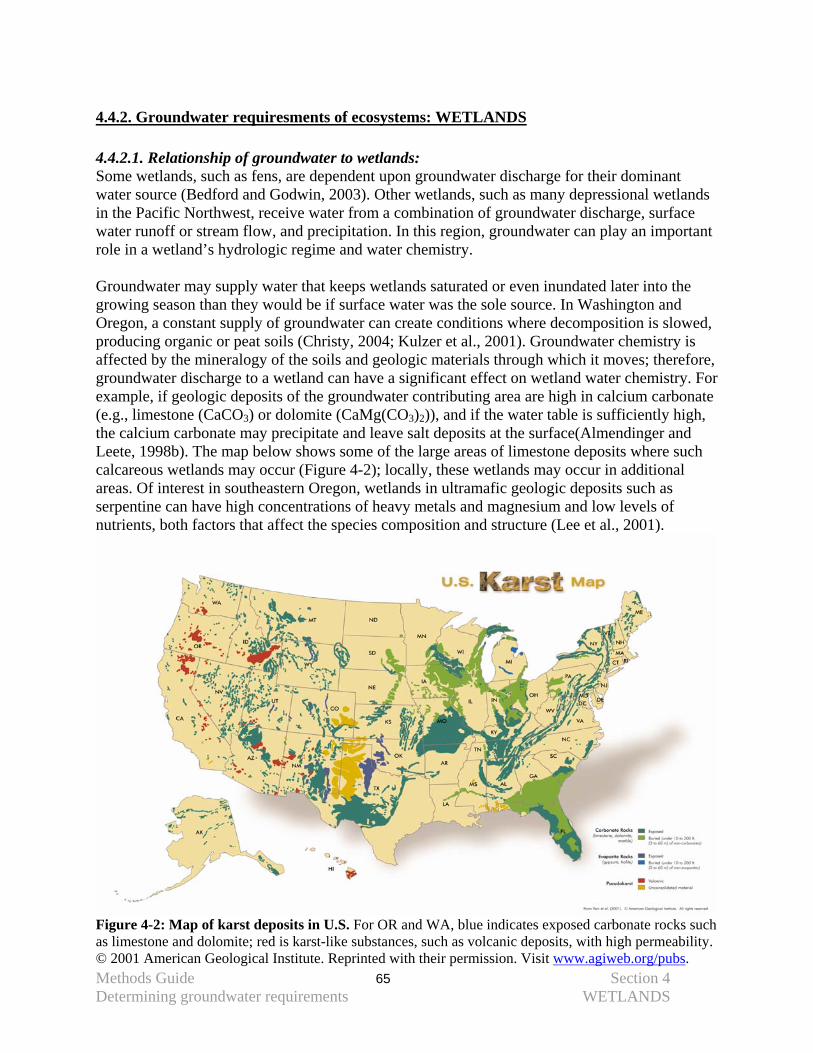
Methods Guide 65 Section 4 Determining groundwater requirements WETLANDS
4.4.2. Groundwater requiresments of ecosystems: WETLANDS 4.4.2.1. Relationship of groundwater to wetlands: Some wetlands, such as fens, are dependent upon groundwater discharge for their dominant water source (Bedford and Godwin, 2003). Other wetlands, such as many depressional wetlands in the Pacific Northwest, receive water from a combination of groundwater discharge, surface water runoff or stream flow, and precipitation. In this region, groundwater can play an important role in a wetland’s hydrologic regime and water chemistry. Groundwater may supply water that keeps wetlands saturated or even inundated later into the growing season than they would be if surface water was the sole source. In Washington and Oregon, a constant supply of groundwater can create conditions where decomposition is slowed, producing organic or peat soils (Christy, 2004; Kulzer et al., 2001). Groundwater chemistry is affected by the mineralogy of the soils and geologic materials through which it moves; therefore, groundwater discharge to a wetland can have a significant effect on wetland water chemistry. For example, if geologic deposits of the groundwater contributing area are high in calcium carbonate (e.g., limestone (CaCO3) or dolomite (CaMg(CO3)2)), and if the water table is sufficiently high, the calcium carbonate may precipitate and leave salt deposits at the surface(Almendinger and Leete, 1998b). The map below shows some of the large areas of limestone deposits where such calcareous wetlands may occur (Figure 4-2); locally, these wetlands may occur in additional areas. Of interest in southeastern Oregon, wetlands in ultramafic geologic deposits such as serpentine can have high concentrations of heavy metals and magnesium and low levels of nutrients, both factors that affect the species composition and structure (Lee et al., 2001).
Figure 4-2: Map of karst deposits in U.S. For OR and WA, blue indicates exposed carbonate rocks such as limestone and dolomite; red is karst-like substances, such as volcanic deposits, with high permeability. © 2001 American Geological Institute. Reprinted with their permission. Visit www.agiweb.org/pubs.
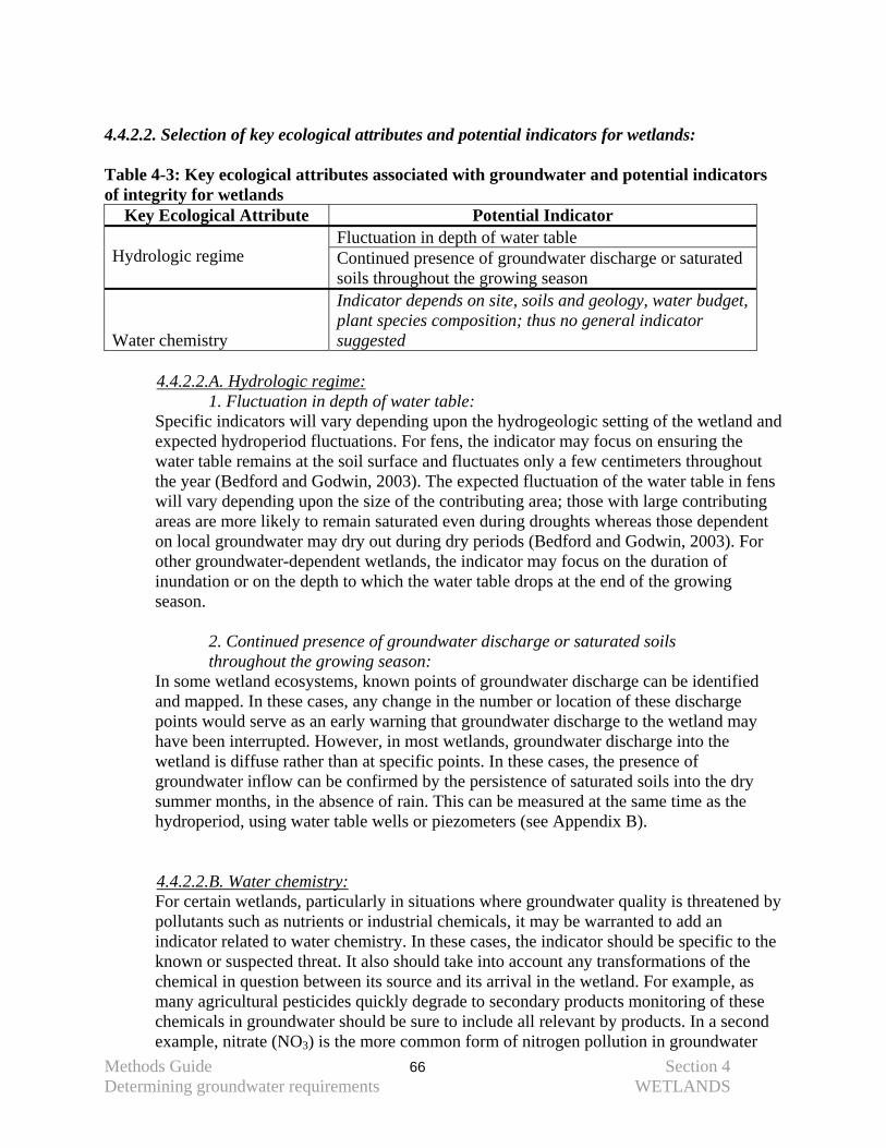
Methods Guide 66 Section 4 Determining groundwater requirements WETLANDS
4.4.2.2. Selection of key ecological attributes and potential indicators for wetlands: Table 4-3: Key ecological attributes associated with groundwater and potential indicators of integrity for wetlands
Key Ecological Attribute Potential Indicator Fluctuation in depth of water table
Hydrologic regime
Continued presence of groundwater discharge or saturated soils throughout the growing season
Water chemistry
Indicator depends on site, soils and geology, water budget, plant species composition; thus no general indicator suggested
4.4.2.2.A. Hydrologic regime:
1. Fluctuation in depth of water table: Specific indicators will vary depending upon the hydrogeologic setting of the wetland and expected hydroperiod fluctuations. For fens, the indicator may focus on ensuring the water table remains at the soil surface and fluctuates only a few centimeters throughout the year (Bedford and Godwin, 2003). The expected fluctuation of the water table in fens will vary depending upon the size of the contributing area; those with large contributing areas are more likely to remain saturated even during droughts whereas those dependent on local groundwater may dry out during dry periods (Bedford and Godwin, 2003). For other groundwater-dependent wetlands, the indicator may focus on the duration of inundation or on the depth to which the water table drops at the end of the growing season.
2. Continued presence of groundwater discharge or saturated soils throughout the growing season:
In some wetland ecosystems, known points of groundwater discharge can be identified and mapped. In these cases, any change in the number or location of these discharge points would serve as an early warning that groundwater discharge to the wetland may have been interrupted. However, in most wetlands, groundwater discharge into the wetland is diffuse rather than at specific points. In these cases, the presence of groundwater inflow can be confirmed by the persistence of saturated soils into the dry summer months, in the absence of rain. This can be measured at the same time as the hydroperiod, using water table wells or piezometers (see Appendix B).
4.4.2.2.B. Water chemistry: For certain wetlands, particularly in situations where groundwater quality is threatened by pollutants such as nutrients or industrial chemicals, it may be warranted to add an indicator related to water chemistry. In these cases, the indicator should be specific to the known or suspected threat. It also should take into account any transformations of the chemical in question between its source and its arrival in the wetland. For example, as many agricultural pesticides quickly degrade to secondary products monitoring of these chemicals in groundwater should be sure to include all relevant by products. In a second example, nitrate (NO3) is the more common form of nitrogen pollution in groundwater
Methods Guide 67 Section 4 Determining groundwater requirements WETLANDS
due to its mobility. However, many wetlands naturally have reducing conditions where the NO3 is immediately transformed to ammonium (NH4), and so it is the NH4 that could be monitored. That said, establishing a water chemistry sampling regime is a complicated and costly endeavor, and so this should be done with significant expert input and a dedicated budget.
In general for a wetland without a specific threat associated with water quality impairment, it is unlikely to be useful to measure water chemistry. Where wetlands have characteristic water chemistry created by the prevalence of minerals (such as calcium, potassium, and magnesium), it may be tempting to add an indicator related to water chemistry. Usually the water chemistry is a function of groundwater flow paths and the quantity of the groundwater discharging into a wetland (e.g., Almendinger and Leete, 1998b). Thus, the hydrologic regime indicators suggested earlier usually are adequate to monitor alterations to these water chemistry conditions.
4.4.2.3. Example: KEA and indicator identification for Coastal Mountain Fen In the coast range of Oregon, small fens often develop in depressions along wetter western slopes. Their water supply is maintained by a mix of groundwater, surface water and precipitation. The groundwater is recharged higher in the watershed, travels through relatively shallow, local aquifers, and discharges at breaks in slope where it pools in depressions, thus promoting the formation of small fens (see Wetlands discussion in Section 3 of this document). Surface water flowing from small mountain streams into the fens also feeds these wetlands. Although these fens are found in a region with high precipitation, groundwater sustains the water table at a relatively stable and high level. This high water table promotes the accumulation of peat (partially decomposed organic matter) because plant decomposition is slowed down by the constantly waterlogged conditions.
Groundwater discharge to these fens also helps to maintain a characteristic water chemistry. Fen water has a low electrical conductivity because the groundwater moves a short distance through bedrock with low solubility. These conditions, and the absence of human activity in the recharge areas, also ensure the fen water has low nutrient concentrations. These factors – continuously saturated soils, peat accumulation, and low nutrient concentrations – support a unique flora and fauna, including Sphagnum mosses, ericaceous shrubs such as Labrador tea, and carnivorous plants such as sundews and bladderwort. The primary key ecological attribute associated with groundwater in this ecosystem is the sustained rate of groundwater discharge into the wetland. It is very difficult to measure discharge across a diffuse area such as a wetland, thus fluctuations in the water table elevation can serve as an indicator for groundwater discharge. Although the amount of fluctuation will depend upon the wetland under consideration, fluctuations should be minimal – for example, annual fluctuations less than 50 cm from the highest water table elevation to the lowest elevation. Changes in the water table elevation can be measured with shallow water table wells. The primary threats to the groundwater discharge are land uses that can alter groundwater recharge and movement in the contributing area, such as logging and road construction. The secondary key ecological attribute is the characteristic water chemistry of these fens, defined by low mineral and nutrient concentrations. While this attribute is a critical element to these

Methods Guide 68 Section 4 Determining groundwater requirements WETLANDS
coastal mountain fens, in the absence of activities such as grazing or the presence of nearby septic systems, it is not likely to change as long as the amount of groundwater discharging to the wetland remains fairly constant. Thus we have not developed an indicator for water chemistry at this site.
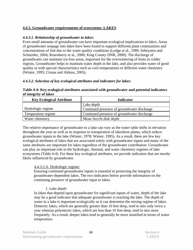
Methods Guide 69 Section 4 Determining groundwater requirements LAKES
4.4.3. Groundwater requiresments of ecosystems: LAKES 4.4.3.1. Relationship of groundwater to lakes: Even small amounts of groundwater can have important ecological implications to lakes. Areas of groundwater seepage into lakes have been found to support different plant communities and concentrations of fish due to the water quality conditions (Lodge et al., 1989, Sebeysten and Schneider, 2004; Rosenberry et al., 2000; King County DNR, 2000). The discharge of groundwater can maintain ice-free areas, important for the overwintering of biota in colder regions. Groundwater helps to maintain water depth in the lake, and also provides water of good quality or with special characteristics such as cool temperatures or different water chemistry (Winter, 1995; Ciruna and Aldous, 2005). 4.4.3.2. Selection of key ecological attributes and indicators for lakes: Table 4-4: Key ecological attributes associated with groundwater and potential indicators of integrity of lakes
Key Ecological Attribute Indicator Lake depth
Hydrologic regime Continued presence of groundwater discharge Temperature regime Continued presence of groundwater discharge Water chemistry Mean Secchi disk depth
The relative importance of groundwater to a lake can vary as the water table shifts in elevation throughout the year as well as in response to transpiration of lakeshore plants, which reduce groundwater inputs to the lake (Winter, 1978; Winter, 1995). As a result, there are few key ecological attributes of lakes that are associated solely with groundwater inputs and many of the same attributes are important for lakes regardless of the groundwater contribution. Groundwater can play an important role in the hydrologic, thermal, and water chemistry regimes of lake ecosystems (Table 4-4). For these key ecological attributes, we provide indicators that are mostly likely influenced by groundwater. 4.4.3.2.A. Hydrologic regime:
Ensuring continued groundwater inputs is essential to protecting the integrity of groundwater-dependent lakes. The two indicators below provide information on the continuing presence of groundwater input to lakes. 1. Lake depth: In lakes that depend upon groundwater for significant inputs of water, depth of the lake may be a good indicator that adequate groundwater is reaching the lake. The depth of water in a lake is important ecologically as it can determine the mixing regime of lakes. Dimectic lakes, which are generally greater than 10 feet deep, tend to mix only twice a year whereas polymectic lakes, which are less than 10 feet deep, tend to mix more frequently. As a result, deeper lakes tend to generally be more stratified in terms of water temperature.
Methods Guide 70 Section 4 Determining groundwater requirements LAKES
As it is unlikely that the depth of a lake remains constant from year to year or throughout a year, it may be more appropriate to identify ‘minimum depth of lake’ or ‘range of lake depth’ as the indicator that the groundwater inputs are intact.
2. Location and continued presence of groundwater discharge:
For lakes where groundwater discharge areas are discrete and can be mapped, it is important to ensure that these areas continue to provide input over time.
4.4.3.2.B. Thermal regime: 1. Location and continued presence of groundwater discharge:
Discrete points of groundwater discharge may also provide thermal refugia for aquatic biota. It is important to ensure that these areas continue to exist over time.
4.4.3.2.C. Water chemistry:
If groundwater provides an important source of water to a lake, then groundwater contaminated by nutrients, such as nitrogen or phosphorus, could increase these concentrations within the lake. Measures of the trophic state of a lake indicate the degree to which a lake is eutrophic or has high nutrient concentrations. Unnatural eutrophic conditions can degrade the condition of a lake by producing excessive growth of aquatic plants and algae, reducing dissolved oxygen levels, killing fish, and shifting the composition or relative abundance of biological communities in the lake (US EPA, 2001). The most complete way to assess the trophic state of a lake would be to follow the protocol suggested by the US EPA (2001) which involves two sets of indicators:
i. measurements of the nutrients that cause eutrophication – total nitrogen and total phosphorus concentrations and
ii. measurements of the response of the lake to increases in nutrients – chlorophyll a concentrations ( as an indicator of algal biomass) and a measure of turbidity. The depth at which a Secchi disk can be seen is one of the easiest ways to assess turbidity.
For each region or sub-ecoregion in the Pacific Northwest, the US EPA (2000, 2001) suggests quantitative desired future conditions for all four of these factors. These values are based upon the lower quartile of values from all monitored lakes in the subregion; these correspond with values from the best reference lakes, according to studies from Minnesota, Tennessee, and New York (US EPA, 2000). There are some complications with using the indicators suggested by the US EPA – measuring nutrient and chlorophyll concentrations is expensive, requires adherence to strict sampling and processing protocols, and the values can vary dramatically between years (Bell-McKinnon, 2002). Therefore, we recommend only measuring turbidity to assess the trophic state of a lake.
1. Secchi disk depth:
Secchi disk readings are a relatively simple measure of the turbidity of a lake, and have a good correlation with chlorophyll a concentrations (Carlson, 1977). In its volunteer monitoring program, the Washington State Department of Ecology collected at least five Secchi disk readings a year at each site between mid May and mid October (Bell-McKinnon, 2002).
Methods Guide 71 Section 4 Determining groundwater requirements LAKES
Desired future conditions can be described in terms of Secchi disk transparency (see the US EPA 2000 and 2001 for suggestions of reasonable values) or in terms of an index termed the Carlson's Trophic State Index (TSI) (Carlson, 1977). Calculations of these TSI values can be obtained from the Washington State Department of Ecology (http://www.ecy.wa.gov/programs/wq/plants/management/joysmanual/lakedata.html).
4.4.3.3. Example: KEA and indicator identification for a Columbia River Basin lake In the Columbia River Basin, the draining of glacial Lake Missoula resulted in the formation of remnant lakes in the gravel, cobble and boulder deposits of the relic river channels. One of these lakes is of conservation concern due to the habitat it provides for migrating and nesting birds as well as amphibians and fish. The lake is hydrologically connected to groundwater. Groundwater enters the lake on the northern side and leaves, recharging the aquifer, on the southern side. The primary key ecological attribute for this lake is the hydrologic regime, specifically the input of groundwater. The amount of groundwater entering the lake has the potential to be altered through groundwater extraction for irrigation of surrounding agricultural lands. Although techniques do exist for measuring groundwater seepage into lakes (Lee, 1977; Winter et al., 1998), they are labor and cost intensive. Instead, the elevation of the shoreline at the end of the summer dry season can be used as an indicator that an adequate lake depth is being maintained. These measurements, taken when surface water inputs have ceased, will ensure that groundwater inputs are providing an adequate water supply. The lake has an average depth of about 5.5 m (18 feet) and generally the shoreline falls between 317 and 329 m (1040 and 1050 feet) in elevation. The minimum desired shoreline elevation for September is set at 317 m. The secondary key ecological attribute for this lake is the water chemistry. The primary threat to the water chemistry is contamination with nutrients from fertilizers, septic systems, and cattle. Since measuring these parameters is expensive and difficult, we use the Secchi disk depth to calculate the trophic status of the lake as an indicator of the nutrient concentrations. Secchi disk depth is measured once a month from April through October. Using the EPA standards for this ecoregion (US EPA, 2001), Secchi disk measurements shall be greater than 2m in order for the lake to be considered relatively unimpaired by nutrients.
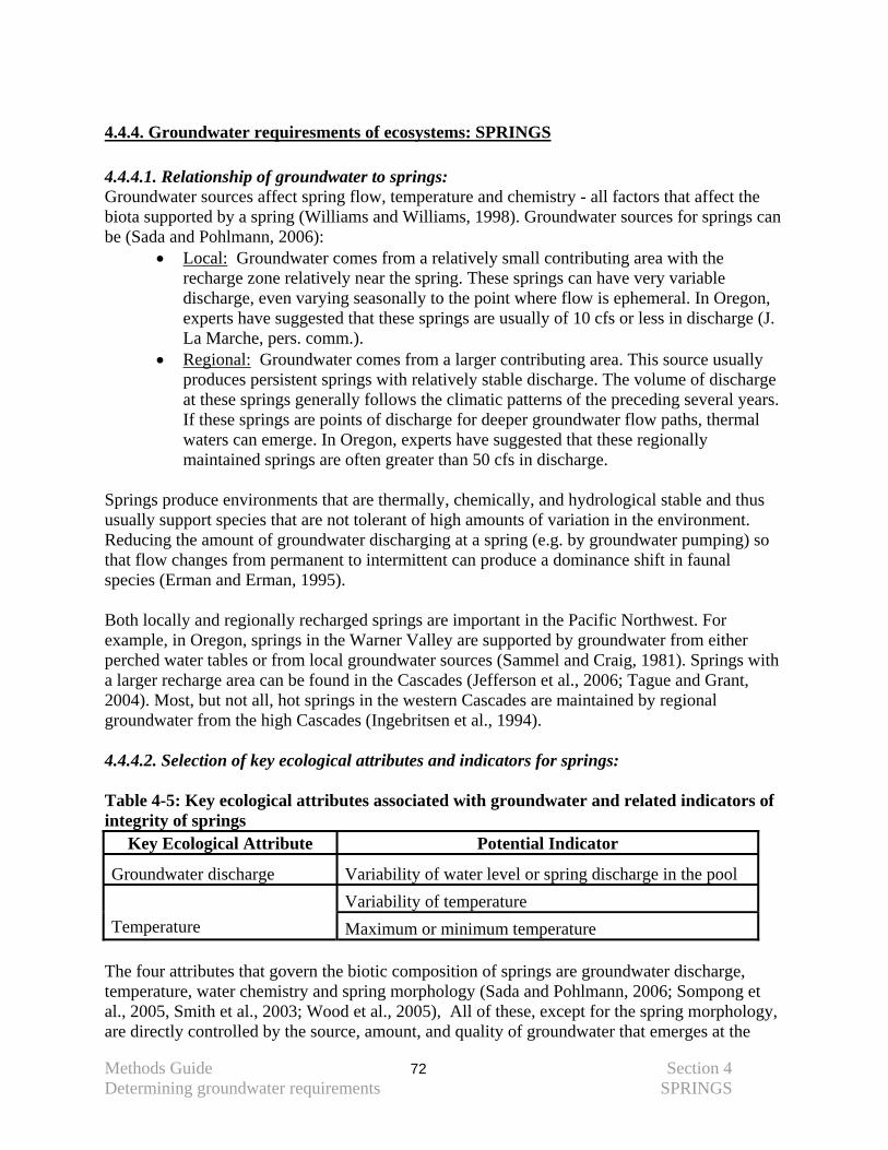
Methods Guide 72 Section 4 Determining groundwater requirements SPRINGS
4.4.4. Groundwater requiresments of ecosystems: SPRINGS 4.4.4.1. Relationship of groundwater to springs: Groundwater sources affect spring flow, temperature and chemistry - all factors that affect the biota supported by a spring (Williams and Williams, 1998). Groundwater sources for springs can be (Sada and Pohlmann, 2006):
• Local: Groundwater comes from a relatively small contributing area with the recharge zone relatively near the spring. These springs can have very variable discharge, even varying seasonally to the point where flow is ephemeral. In Oregon, experts have suggested that these springs are usually of 10 cfs or less in discharge (J. La Marche, pers. comm.).
• Regional: Groundwater comes from a larger contributing area. This source usually produces persistent springs with relatively stable discharge. The volume of discharge at these springs generally follows the climatic patterns of the preceding several years. If these springs are points of discharge for deeper groundwater flow paths, thermal waters can emerge. In Oregon, experts have suggested that these regionally maintained springs are often greater than 50 cfs in discharge.
Springs produce environments that are thermally, chemically, and hydrological stable and thus usually support species that are not tolerant of high amounts of variation in the environment. Reducing the amount of groundwater discharging at a spring (e.g. by groundwater pumping) so that flow changes from permanent to intermittent can produce a dominance shift in faunal species (Erman and Erman, 1995). Both locally and regionally recharged springs are important in the Pacific Northwest. For example, in Oregon, springs in the Warner Valley are supported by groundwater from either perched water tables or from local groundwater sources (Sammel and Craig, 1981). Springs with a larger recharge area can be found in the Cascades (Jefferson et al., 2006; Tague and Grant, 2004). Most, but not all, hot springs in the western Cascades are maintained by regional groundwater from the high Cascades (Ingebritsen et al., 1994). 4.4.4.2. Selection of key ecological attributes and indicators for springs: Table 4-5: Key ecological attributes associated with groundwater and related indicators of integrity of springs
Key Ecological Attribute Potential Indicator
Groundwater discharge Variability of water level or spring discharge in the pool Variability of temperature
Temperature Maximum or minimum temperature The four attributes that govern the biotic composition of springs are groundwater discharge, temperature, water chemistry and spring morphology (Sada and Pohlmann, 2006; Sompong et al., 2005, Smith et al., 2003; Wood et al., 2005), All of these, except for the spring morphology, are directly controlled by the source, amount, and quality of groundwater that emerges at the
Methods Guide 73 Section 4 Determining groundwater requirements SPRINGS
spring and have been selected as the key ecological attributes associated with groundwater that govern spring integrity (Table 4-4). 4.4.4.2.A Groundwater discharge:
The expected volume of groundwater that discharges to a spring is important for maintaining the viability of the spring and supporting the associated biota. 1. Variability of water table level or spring discharge in the pool:
Measuring the discharge at a spring using conventional river flow measurement techniques is difficult (Sada and Pohlmann, 2006). Since springs are often too shallow to use flow meters, Sada and Pohlmann recommend using a bottle of a known size (e.g. 500 ml) and recording the time it takes for the bottle to fill. If this is not feasible, the water table level or depth of water at the spring source could instead be measured.
The variability of discharge to springs is related to the source of groundwater (Sada et al., 2001) thus different indicators may be necessary depending upon the source of water to the spring. For ephemeral springs, the indicator may be the year to year variability of the water table level from early spring to mid summer. For more permanent springs, within year (seasonal) variability might be measured as well as between year variability.
4.4.4.2.B. Temperature:
1. Variability of temperature:
Temperature in both hot and cold springs is fairly constant (Galas, 2005). Cold springs are those with temperatures below or near mean annual air temperature, thermal springs are 5-10°C (9 – 18°F) above mean annual air temperature, and hot springs are more than 10°C (18° F) above mean annual air temperature (Sada et al., 2001). The temperature of cool water springs likely reflects that of the mean air temperature at the elevation of initial recharge. Hot water, found in thermal and hot springs, results as water is heated geothermally when it circulates more deeply.
Temperature should be measured near the source of the spring. Determining the desired variability of the temperature of spring water may be difficult but there are likely some studies that can help define a reasonable objective. For example, work in Ontario found that increasing spring water temperature (in coldwater springs) by 2-3.5°C (3.6-6.3°F) produced drastic changes in the invertebrate community; species composition, timing of reproduction and sex ratios of different species changed as a result (Hogg and Williams, 1996).
2. Minimum or maximum temperature:
The temperature of a spring plays a very important role in structuring its biotic community. Temperatures greater than about 45°C (113°F ) are too high for fish and macroinvertebrate species to be present and the community is dominated by microbes that tolerate the extreme conditions (Sada unpublished). In Thai hot springs, diversity of cyanobacteria decreased as temperature of water increased until only heat tolerant species remained (Sompong et al., 2005). At temperatures higher than 70°C (158°F), photosynthesis is reported to cease (Spear et al., 2005). In hot springs, Breitbart et al.
Methods Guide 74 Section 4 Determining groundwater requirements SPRINGS
(2004) found that viruses (phages) can tolerate shifts to warmer temperatures; as temperatures drop, other microbes thrive and viruses are less dominant in the hot springs community.
4.4.4.3. Example: KEA and indicator identification for eastern Cascade spring Springs are abundant on the eastern slope of the Cascades in Oregon. One spring in particular is considered important as it provides flow to the lower three miles of a creek used by rearing bull trout and spawning resident redband trout. This flow not only keeps stream temperatures cool but it also maintains a lush riparian area in this otherwise very arid environment. The recharge for this spring is likely from snowmelt on the permeable geologic deposits of mountain slopes in the upper part of the watershed. Water percolates down through permeable volcanic deposits until it reaches a layer that is underlain by a less permeable, older volcanic material. Then, following the general downward topographic gradient of the land surface, this water moves down the watershed within the permeable layer until it is exposed at the base of a canyon wall and emerges as a spring adjacent to the creek. The primary key ecological attribute for this spring is the discharge of groundwater. There is great potential for this attribute to be altered by groundwater extraction (i.e. pumping) between the recharge area and the spring. The creek below the spring is not gaged and it is difficult to measure discharge from the spring; however, as the spring emerges into a pool, the water level of the pool can be used as an indicator of groundwater discharge. The pool water level can be measured and recorded by electronic water level recording devices or by manually reading a staff gage once every two weeks. As the water level is expected to remain fairly constant, we would like to see variability of no more than 10 cm throughout a year and between years at this particular spring. There are no data available to help us set this objective; instead, we hope to have selected a value that will provide an early warning if the supply of groundwater to the spring is changing. A secondary key ecological attribute is water temperature. One primary threat to this is climate change which could increase the air temperature in the recharge area; if this happened, the water temperature from the spring could be raised. Temperature at the discharge point can be measured using a recording temperature sensor. Values should range from 13-14°C, or 55-57°F, year round.
Methods Guide 75 Section 4 Determining groundwater requirements PHREATOPHYTES
4.4.5. Groundwater requiresments of ecosystems: PHREATOPHYTIC ECOSYSTEMS 4.4.5.1. Relationship of groundwater to phreatophytic ecosystems: A species can be phreatophytic, and therefore depend on groundwater for its water supply, if it uses this deeper water constantly, seasonally, or only episodically (e.g. during extended dry periods) (Zencich and Froend, 2001). Some phreatophytes are facultatively dependent upon groundwater, using it in certain environments but not in others (Naiman et al., 2006). In some arid areas, a species may not absolutely require the presence of groundwater but it may grow more vigorously if groundwater is available, as individuals are less water stressed (Naumberg et al., 2005; Stromberg et al., 1996). There are two landscape settings in which phreatophytes tend to occur: upland areas, usually in arid or semi-arid conditions, and riparian areas.
• Upland setting: Plants in upland settings have two potential sources of water: the soil moisture and groundwater. The importance of groundwater is generally determined by three factors: i) the proximity of groundwater to plants (i.e. water table depth) ii) the availability of shallow soil water and iii) the distribution of roots, including rooting depth.
• Riparian setting: Although plants growing in riparian areas have access to river or stream water (O’Grady et al., 2006), several riparian species have been identified that use groundwater rather than streamwater as their water supply (Dawson and Ehleringer, 1991).
Even though phreatophytes are identified on a species by species basis, there is growing evidence to suggest that the presence of some phreatophytes may play an important role in water availability during summer droughts for surrounding shallow-rooted species and perhaps the larger ecosystem. In the past decade, studies have found that over 60 species (Jackson et al., 2000) redistribute water accessed by deep roots into shallower parts of the soil profile. This water is then used by shallow rooted plants and seedlings (Caldwell et al., 1998) and can provide up to half of the subsequent day’s water for transpiration by some plants (Naumberg et al., 2005). There is evidence that this may be important even in less arid environments. In the western portion of Pacific Northwest (Gifford Pinchot Wind River area), studies have found that up to 28 percent of the water in the upper layers of soil profiles was groundwater that had been redistributed by Douglas fir (Brooks et al., 2002). The importance of this phenomenon from an ecosystem perspective is still being studied.
Methods Guide 76 Section 4 Determining groundwater requirements PHREATOPHYTES
4.4.5.2. Explanation of selection of key ecological attributes and indicators for phreatophytes: Table 4-6: Key ecological attributes associated with groundwater and potential indicators of integrity of phreatophytic ecosystems
Key Ecological Attribute Indicator Maximum water table depth Maximum rate at which water table drops
Hydrologic regime Timing of drop in water table 4.4.5.2.A Hydrologic regime:
The hydrologic regime is the key ecological attribute associated with groundwater that is relevant to phreatophytes. Phreatophytes, either facultative or obligate, depend upon groundwater to prevent water stress. Water stress can lead to a change in plant condition and/or reduced vigor or mortality of leaves, branches or entire plants. Suggested indicators of the condition of the hydrologic regime for phreatophytes are all related to the water table level and how and when it changes. Naumberg et al. (2005) developed a flow chart that indicates the conditions under which these changes would be expected to affect phreatophytic ecosystems (Figure 4-3). This framework provides a guide for identifying indicators of the hydrologic regime that are relevant to phreatophytes. 1. Maximum water table depth: The depth of the water table is critical to whether groundwater can provide water to phreatophytic plants. However, the water table is rarely static even under natural conditions. As a result it is the maximum depth of the water table during the growing season that may be a good indicator of the availability of groundwater to phreatophytic ecosystems. Some guidelines on depths of specific species can be found in review articles such as Jackson et al. (1996) and Stone and Kalisz (1991).
2. Maximum rate at which water table drops:
If the water table declines at a rate that is too fast, then plant roots may be unable to adjust. Studies have documented root growth rates for some species; for example, cottonwood, willow and tamarisk seedling roots grow at 1-13 mm/d and arid shrub roots can grow at 3-15 mm/d (Naumberg et al., 2005). The adaptability of different species to changing water tables is variable. Some species such as Artemisia tridentata, can shift from using groundwater when summer precipitation is available as they maintain both deep and shallow roots throughout the growing season. Other species, for example, Chrysothamnus nausesosus, only maintain active roots in deeper soil and so are unable to shift water sources even when significant summer precipitation occurs. Additionally, the effect on plants may be reduced (i.e. the water stress may be less severe) if the species are arid plants which are more tolerant of water stress, or if the soils are fine, thus able to hold more water even as the groundwater drops. 3. Timing of drop in water table: A drop in the water table only affects a phreatophyte if the water level drops below the rooting depth during the growing season. As a result, understanding the physiology and ecology of the phreatophytic species is essential to developing objectives for water table management.
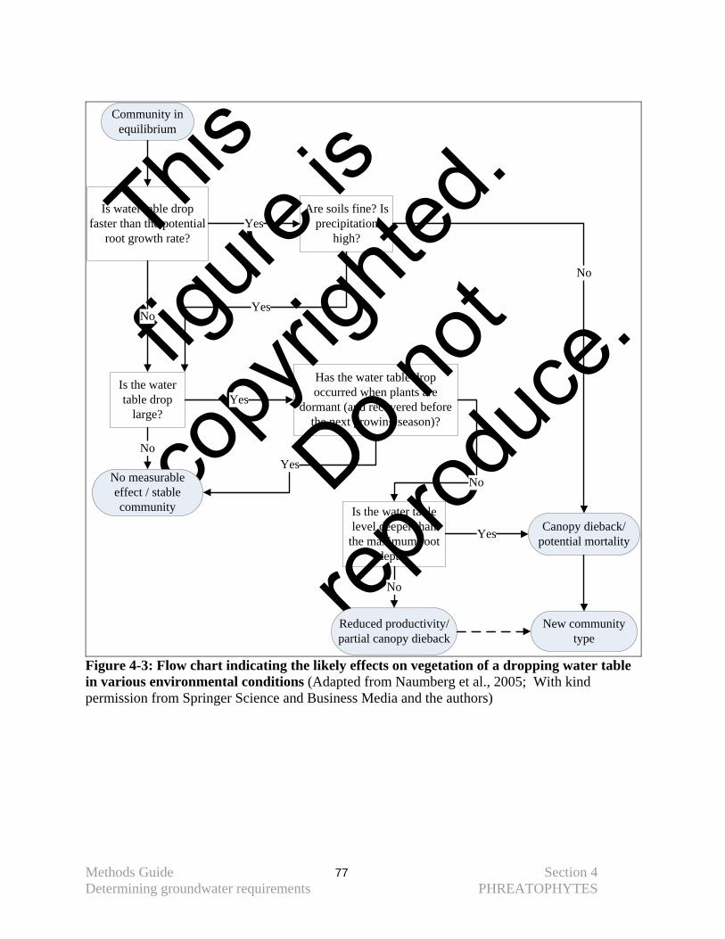
This
figure
is
copy
righte
d.
Do not
reprod
uce.
Methods Guide 77 Section 4 Determining groundwater requirements PHREATOPHYTES
Community in
equilibrium
Is water table drop faster than the potential
root growth rate?
Are soils fine? Is precipitation
high?Yes
Is the water table drop
large?
No
Is the water table level deeper than
the maximum root depth?
Yes
No measurable effect / stable community
No
Reduced productivity/partial canopy dieback
No
Yes
Canopy dieback/potential mortality
New community type
Yes
No
Has the water table drop occurred when plants are
dormant (and recovered before the next growing season)?
YesNo
Figure 4-3: Flow chart indicating the likely effects on vegetation of a dropping water table in various environmental conditions (Adapted from Naumberg et al., 2005; With kind permission from Springer Science and Business Media and the authors)
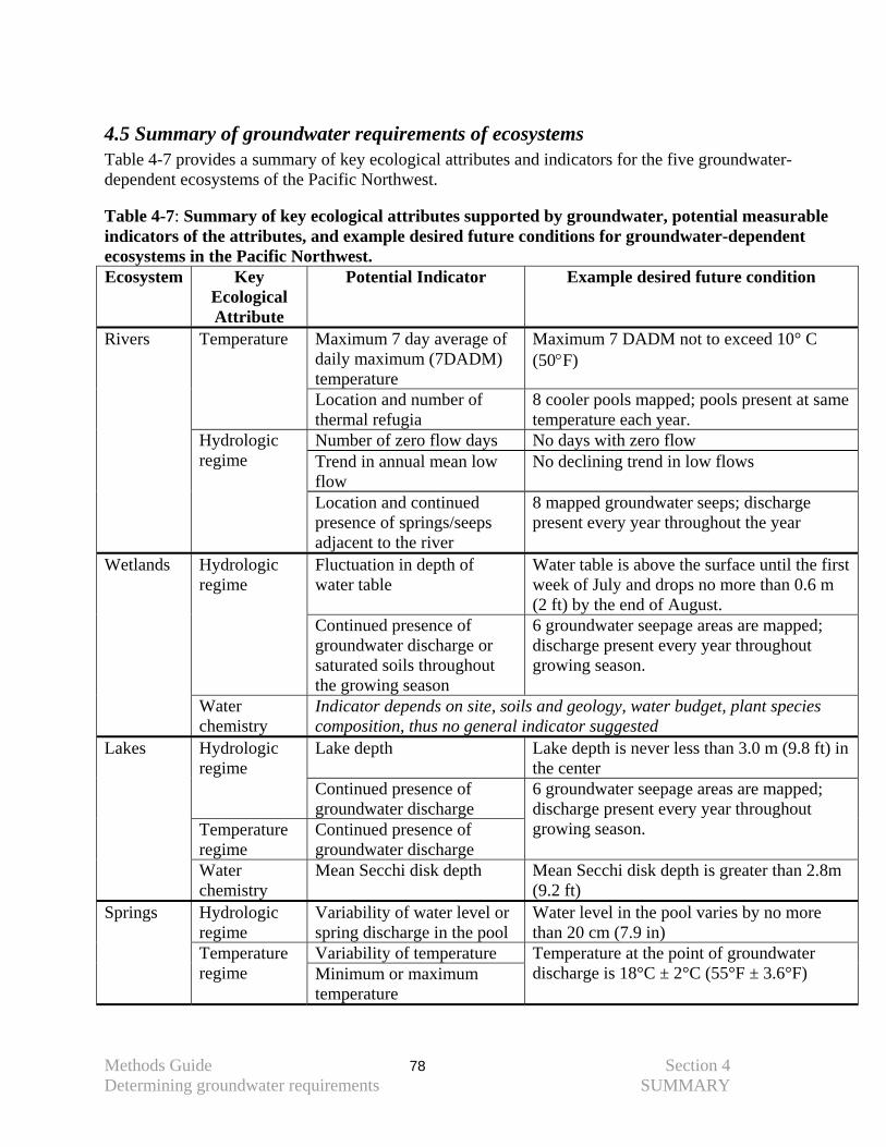
Methods Guide 78 Section 4 Determining groundwater requirements SUMMARY
4.5 Summary of groundwater requirements of ecosystems Table 4-7 provides a summary of key ecological attributes and indicators for the five groundwater-dependent ecosystems of the Pacific Northwest. Table 4-7: Summary of key ecological attributes supported by groundwater, potential measurable indicators of the attributes, and example desired future conditions for groundwater-dependent ecosystems in the Pacific Northwest. Ecosystem Key
Ecological Attribute
Potential Indicator Example desired future condition
Maximum 7 day average of daily maximum (7DADM) temperature
Maximum 7 DADM not to exceed 10° C (50°F)
Temperature
Location and number of thermal refugia
8 cooler pools mapped; pools present at same temperature each year.
Number of zero flow days No days with zero flow Trend in annual mean low flow
No declining trend in low flows
Rivers
Hydrologic regime
Location and continued presence of springs/seeps adjacent to the river
8 mapped groundwater seeps; discharge present every year throughout the year
Fluctuation in depth of water table
Water table is above the surface until the first week of July and drops no more than 0.6 m (2 ft) by the end of August.
Hydrologic regime
Continued presence of groundwater discharge or saturated soils throughout the growing season
6 groundwater seepage areas are mapped; discharge present every year throughout growing season.
Wetlands
Water chemistry
Indicator depends on site, soils and geology, water budget, plant species composition, thus no general indicator suggested Lake depth Lake depth is never less than 3.0 m (9.8 ft) in
the center Hydrologic regime
Continued presence of groundwater discharge
Temperature regime
Continued presence of groundwater discharge
6 groundwater seepage areas are mapped; discharge present every year throughout growing season.
Lakes
Water chemistry
Mean Secchi disk depth Mean Secchi disk depth is greater than 2.8m (9.2 ft)
Hydrologic regime
Variability of water level or spring discharge in the pool
Water level in the pool varies by no more than 20 cm (7.9 in)
Variability of temperature
Springs
Temperature regime Minimum or maximum
temperature
Temperature at the point of groundwater discharge is 18°C ± 2°C (55°F ± 3.6°F)
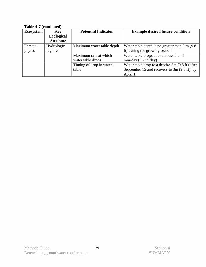
Methods Guide 79 Section 4 Determining groundwater requirements SUMMARY
Table 4-7 (continued) Ecosystem Key
Ecological Attribute
Potential Indicator Example desired future condition
Maximum water table depth Water table depth is no greater than 3 m (9.8 ft) during the growing season
Maximum rate at which water table drops
Water table drops at a rate less than 5 mm/day (0.2 in/day)
Phreato-phytes
Hydrologic regime
Timing of drop in water table
Water table drop to a depth> 3m (9.8 ft) after September 15 and recovers to 3m (9.8 ft) by April 1
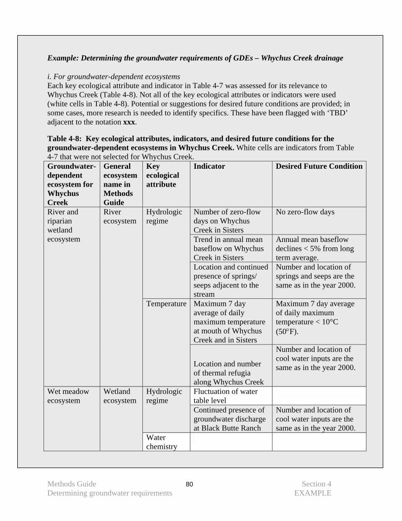
Methods Guide 80 Section 4 Determining groundwater requirements EXAMPLE
Example: Determining the groundwater requirements of GDEs – Whychus Creek drainage i. For groundwater-dependent ecosystems Each key ecological attribute and indicator in Table 4-7 was assessed for its relevance to Whychus Creek (Table 4-8). Not all of the key ecological attributes or indicators were used (white cells in Table 4-8). Potential or suggestions for desired future conditions are provided; in some cases, more research is needed to identify specifics. These have been flagged with ‘TBD’ adjacent to the notation xxx. Table 4-8: Key ecological attributes, indicators, and desired future conditions for the groundwater-dependent ecosystems in Whychus Creek. White cells are indicators from Table 4-7 that were not selected for Whychus Creek. Groundwater-dependent ecosystem for Whychus Creek
General ecosystem name in Methods Guide
Key ecological attribute
Indicator Desired Future Condition
Number of zero-flow days on Whychus Creek in Sisters
No zero-flow days
Trend in annual mean baseflow on Whychus Creek in Sisters
Annual mean baseflow declines < 5% from long term average.
Hydrologic regime
Location and continued presence of springs/ seeps adjacent to the stream
Number and location of springs and seeps are the same as in the year 2000.
Maximum 7 day average of daily maximum temperature at mouth of Whychus Creek and in Sisters
Maximum 7 day average of daily maximum temperature < 10°C (50°F).
River and riparian wetland ecosystem
River ecosystem
Temperature
Location and number of thermal refugia along Whychus Creek
Number and location of cool water inputs are the same as in the year 2000.
Fluctuation of water table level
Hydrologic regime
Continued presence of groundwater discharge at Black Butte Ranch
Number and location of cool water inputs are the same as in the year 2000.
Wet meadow ecosystem
Wetland ecosystem
Water chemistry
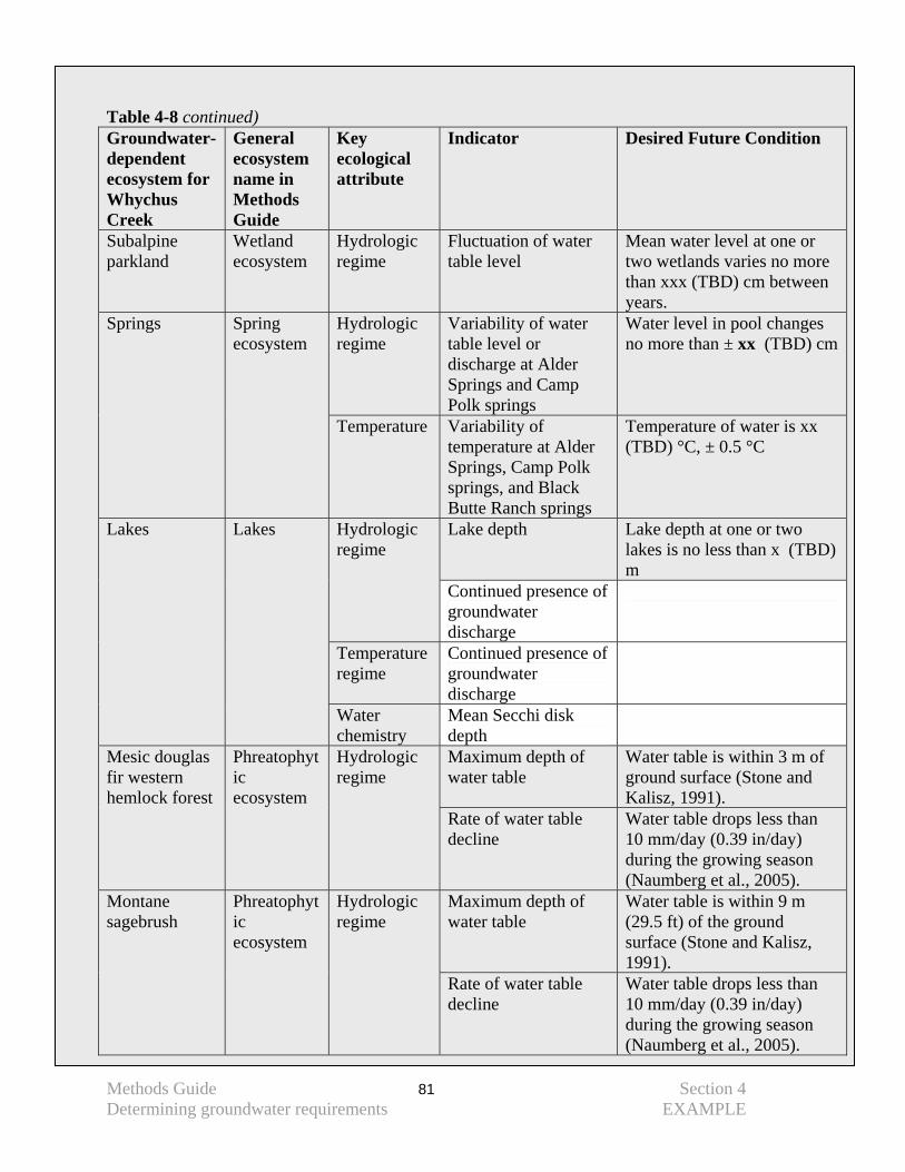
Methods Guide 81 Section 4 Determining groundwater requirements EXAMPLE
Table 4-8 continued) Groundwater-dependent ecosystem for Whychus Creek
General ecosystem name in Methods Guide
Key ecological attribute
Indicator Desired Future Condition
Subalpine parkland
Wetland ecosystem
Hydrologic regime
Fluctuation of water table level
Mean water level at one or two wetlands varies no more than xxx (TBD) cm between years.
Hydrologic regime
Variability of water table level or discharge at Alder Springs and Camp Polk springs
Water level in pool changes no more than ± xx (TBD) cm
Springs Spring ecosystem
Temperature Variability of temperature at Alder Springs, Camp Polk springs, and Black Butte Ranch springs
Temperature of water is xx (TBD) °C, ± 0.5 °C
Lake depth Lake depth at one or two lakes is no less than x (TBD) m
Hydrologic regime
Continued presence of groundwater discharge
Temperature regime
Continued presence of groundwater discharge
Lakes Lakes
Water chemistry
Mean Secchi disk depth
Maximum depth of water table
Water table is within 3 m of ground surface (Stone and Kalisz, 1991).
Mesic douglas fir western hemlock forest
Phreatophytic ecosystem
Hydrologic regime
Rate of water table decline
Water table drops less than 10 mm/day (0.39 in/day) during the growing season (Naumberg et al., 2005).
Maximum depth of water table
Water table is within 9 m (29.5 ft) of the ground surface (Stone and Kalisz, 1991).
Montane sagebrush
Phreatophytic ecosystem
Hydrologic regime
Rate of water table decline
Water table drops less than 10 mm/day (0.39 in/day) during the growing season (Naumberg et al., 2005).
Methods Guide 82 Section 4 Determining groundwater requirements EXAMPLE
ii. For groundwater-dependent species: Species were not addressed individually for the Whychus Creek drainage. The groundwater requirements of individual species were assumed to be addressed by the requirements of the ecosystems in which they occur.
Methods Guide 83 Section 5 Groundwater flow system 5.1 CONTRIBUTING AREA
5. UNDERSTANDING GROUNDWATER FLOW SYSTEMS Conservation of Groundwater Dependent Ecosystems depends upon protecting the quantity and quality of groundwater. The sources of groundwater that support these GDEs may be located a significant distance from the GDE, and movement of water from the source to the GDE may occur over long periods of time (i.e., decades to centuries). This supply can be interrupted or altered by human activities. The first step to protecting GDEs is to develop an understanding of where the groundwater comes from and how it moves from these areas to the GDEs. This section provides guidance for resource managers to develop an initial description of the groundwater system that is important to GDEs at a particular site. Groundwater systems are complex, and developing a robust hypothesis of how a groundwater flow system works may require consultation with professional hydrogeologists, detailed site-level study, and potentially the application of groundwater models. The analysis methods described in this section are meant to provide an initial cut at understanding the groundwater system, and may require review and refinement by experts. The analysis steps described in this section are to: 1) Define the area that contributes groundwater to the GDEs – termed the contributing area 2) Delineate groundwater recharge areas 3) Develop a hypothesis of the patterns of groundwater movement, both horizontal and vertical 4) Develop a general description of how groundwater moves from recharge areas to GDEs, and predict places where groundwater extraction or contamination may pose a significant ecological threat
5.1 The contributing area: The groundwater contributing area describes the parts of the landscape through which groundwater moves as it travels from recharge areas to GDEs and other discharge areas. Often the contributing area matches the surface watershed; however, there are cases where groundwater crosses surface water divides. In these cases, the area contributing groundwater to a GDE is larger than the surface watershed. Human activities within the contributing area have the potential to alter either the quantity or quality of groundwater, therefore understanding its spatial extent is important for identifying potential impacts. The boundary of the contributing area is developed initially by using surface watershed boundaries. If permeable geologic deposits extend beyond the surface watershed, it is possible that the contributing area extends beyond the surface watershed. Surface watershed boundaries and groundwater contributing areas are least likely to be coincident in smaller watersheds; however, even in larger watersheds it is possible for the contributing area to exceed the surface watershed. There are no general rules for determining the extent of the area contributing groundwater, so experts should be consulted to refine this initial delineation.
Methods Guide 84 Section 5 Groundwater flow system 5.1 CONTRIBUTING AREA
Example: Delineating the contributing area: Whychus Creek drainage To identify the contributing area for GDEs in the Whychus Creek drainage, we reviewed the topography (Figure 5-1) and permeability of surficial geologic deposits (Figure 5-2) across the much larger area of the Deschutes River Basin. In general, we looked for evidence that groundwater might enter the Whychus drainage from outside of the surface watershed (red line on Figures 5-1 and 5-2). In this case (Figure 5-2), all of the surficial geologic deposits – alluvium, sedimentary deposits, glacial outwash, and volcanic deposits – within the Whychus Creek watershed are highly permeable and extend outside of the watershed. This would suggest that the contributing area for groundwater may not coincide with the surface watershed. However, consultation with hydrogeologists familiar with this area led us to conclude that in these volcanic deposits, groundwater generally follows surface-topographic patterns. As a result, we assumed that the contributing area matched the surface watershed. This demonstrates the importance of expert review in this process.
Figure 5-1: Topography of the Deschutes Basin and Whychus Creek watershed (USGS, 2006).
Methods Guide 85 Section 5 Groundwater flow system 5.1 CONTRIBUTING AREA
Figure 5-2. General geology of the Deschutes Basin and Whychus Creek watershed (Walker and MacCleod, 1991; mapped classes assigned by the Conservancy).
Methods Guide 86 Section 5 Groundwater flow system 5.2 RECHARGE AREAS
5.2 Recharge areas: Recharge areas (see Section 2.3) are those places in the contributing area where water enters the groundwater system. Recharge areas are particularly susceptible to activities that impair groundwater quantity and quality. Construction of impervious surfaces such as roads, parking lots and buildings can prevent precipitation from infiltrating into the ground and recharging groundwater. Contaminants, such as nutrients from septic systems, can readily enter aquifers through the more permeable deposits located in recharge areas. Generally recharge zones are areas of higher precipitation and more permeable soil and rock types than other parts of the contributing area. An initial guess as to the locations of recharge areas can be made using readily available GIS datalayers. These locations should then be refined through consultation with a hydrogeologist and, possibly, groundwater modeling techniques. Using GIS data: Recharge areas are initially predicted using two data layers: surficial geology and precipitation. This analysis requires identifying areas with: 1) higher permeability. and 2) higher precipitation. The analysis should be conducted over the entire contributing area.
• Locate geologic deposits with higher permeability:
Surficial deposits can be classified according to their relative permeability, and those areas with more permeable deposits are most likely to support groundwater recharge. Assessment of permeability can be based on readily available geology data layers; however, the assessment should be refined with higher resolution data, if available. In Appendix E we describe some general rules for assigning relative permeability characteristics to the geologic deposits of the Oregon statewide surficial geology map. Where higher resolution local geology maps exist, the general rules outlined in the appendix can be applied to obtain better predictions of permeability. In addition, if information on fractures and faulting in the geologic deposits is available, it can also be used to identify areas more likely to support recharge. Assessment of permeability should be reviewed by people familiar with local geologic conditions.
• Locate areas with more precipitation:
Areas with higher precipitation have a greater potential for recharging groundwater. To create a map of precipitation patterns, isohyetals for Oregon and Washington can be obtained from the Oregon Climate Service’s PRISM group at http://www.ocs.orst.edu/prism/products/matrix.phtml?vartype=ppt&view=data and http://www.ocs.orst.edu/prism/state_products/maps.phtml?id=WA
An overlay of the above two datalayers will identify areas with highly permeable geologic deposits and high precipitation, which can be areas likely to provide significant recharge. Other areas may provide some recharge but they tend to be less significant in their groundwater contribution. Refining predictions with models:

Methods Guide 87 Section 5 Groundwater flow system 5.2 RECHARGE AREAS
In some circumstances, a more certain prediction of recharge areas may be required in order to understand the potential threat posed by specific activities in a watershed. Models that predict recharge areas may be useful for meeting this need. One example of this is the Deep Percolation Model (Bauer and Vaccaro, 1987), which has been used in several parts of the Pacific Northwest to predict and map recharge areas. This model and its data requirements are described in more detail in Appendix D.
Methods Guide 88 Section 5 Groundwater flow system 5.2 RECHARGE AREAS: Example
Example: Identifying recharge areas: Whychus Creek drainage
i. Using GIS data: • Locate highly permeable geologic deposits:
In the Deschutes, we began by assessing the relative permeability of surficial geologic deposits using the statewide geology coverage for Oregon and assigning levels of permeability (i.e. high or low) according to Table E-4 (in Appendix E). As a result, 23 deposits were identified as highly permeable deposits (Table 5-1). Based on this, we produced an initial map of the more permeable deposits for the entire basin (Figure 5-3).
Table 5-1: High permeability geologic deposits in the Whychus Creek watershed. (From Walker and MacLeod, 1991)
Map symbol Geologic deposit type Qa Andesite Qal Alluvial deposits Qb Basalt and basaltic andesite Qba Basaltic andesite and basalt Qd Dune sand Qf Fanglomerate Qgf Glaciofluvial deposits Qma Mazama ash flow deposits Qmp Mazama pumice deposits Qrd Rhyolite and dacite Qt Terrace, pediment, and lag gravels QTa Andesite QTb Basalt QTba Basalt and basaltic andesite QTg Terrace gravels QTmv Mafic vent complexes QTp Basaltic and andesitic ejecta QTps Subaqueous basaltic and andesitic ejecta QTst Tuffaceous sedimentary rocks and tuffs QTvm Mafic vent deposits QTvs Silicic vent deposits Qyb Youngest basalt and basaltic andesite
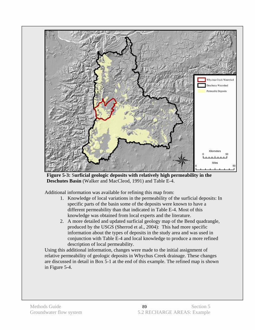
Methods Guide 89 Section 5 Groundwater flow system 5.2 RECHARGE AREAS: Example
Figure 5-3: Surficial geologic deposits with relatively high permeability in the Deschutes Basin (Walker and MacCleod, 1991) and Table E-4.
Additional information was available for refining this map from:
1. Knowledge of local variations in the permeability of the surficial deposits: In specific parts of the basin some of the deposits were known to have a different permeability than that indicated in Table E-4. Most of this knowledge was obtained from local experts and the literature.
2. A more detailed and updated surficial geology map of the Bend quadrangle, produced by the USGS (Sherrod et al., 2004): This had more specific information about the types of deposits in the study area and was used in conjunction with Table E-4 and local knowledge to produce a more refined description of local permeability.
Using this additional information, changes were made to the initial assignment of relative permeability of geologic deposits in Whychus Creek drainage. These changes are discussed in detail in Box 5-1 at the end of this example. The refined map is shown in Figure 5-4.
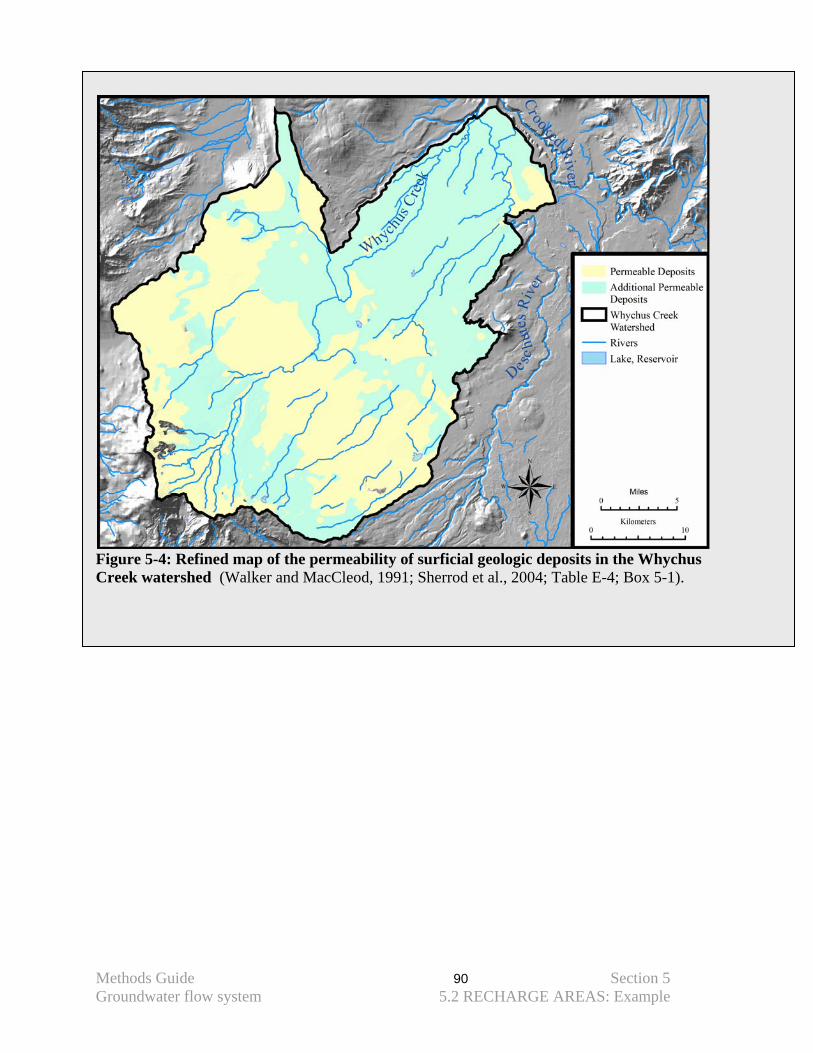
Methods Guide 90 Section 5 Groundwater flow system 5.2 RECHARGE AREAS: Example
Figure 5-4: Refined map of the permeability of surficial geologic deposits in the Whychus Creek watershed (Walker and MacCleod, 1991; Sherrod et al., 2004; Table E-4; Box 5-1).
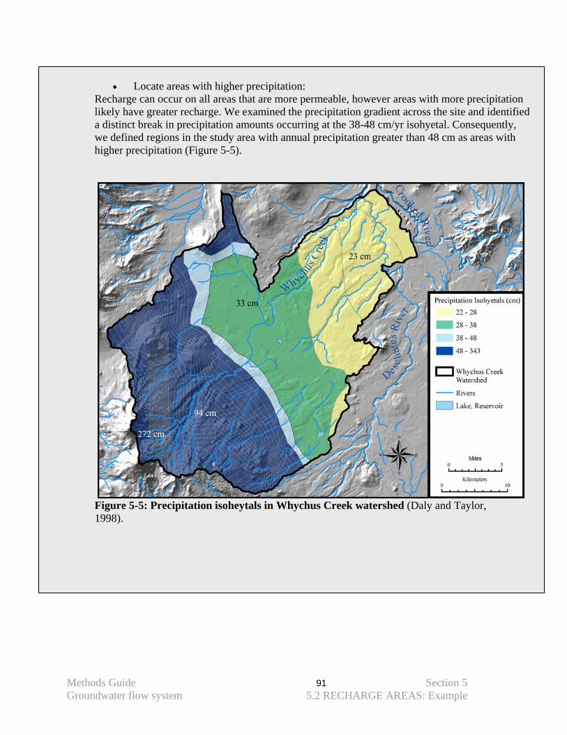
Methods Guide 91 Section 5 Groundwater flow system 5.2 RECHARGE AREAS: Example
• Locate areas with higher precipitation:
Recharge can occur on all areas that are more permeable, however areas with more precipitation likely have greater recharge. We examined the precipitation gradient across the site and identified a distinct break in precipitation amounts occurring at the 38-48 cm/yr isohyetal. Consequently, we defined regions in the study area with annual precipitation greater than 48 cm as areas with higher precipitation (Figure 5-5).
Figure 5-5: Precipitation isoheytals in Whychus Creek watershed (Daly and Taylor, 1998).
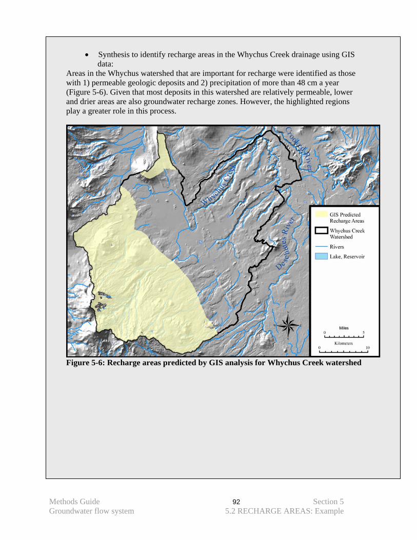
Methods Guide 92 Section 5 Groundwater flow system 5.2 RECHARGE AREAS: Example
• Synthesis to identify recharge areas in the Whychus Creek drainage using GIS data:
Areas in the Whychus watershed that are important for recharge were identified as those with 1) permeable geologic deposits and 2) precipitation of more than 48 cm a year (Figure 5-6). Given that most deposits in this watershed are relatively permeable, lower and drier areas are also groundwater recharge zones. However, the highlighted regions play a greater role in this process.
Figure 5-6: Recharge areas predicted by GIS analysis for Whychus Creek watershed
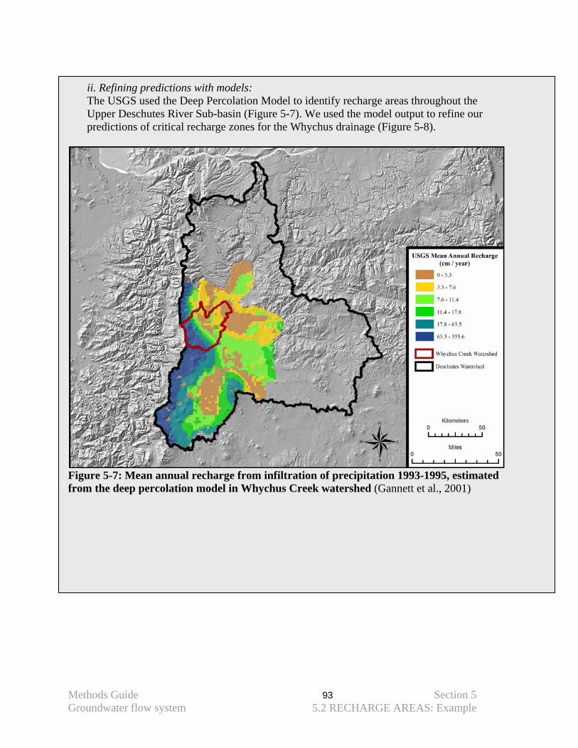
Methods Guide 93 Section 5 Groundwater flow system 5.2 RECHARGE AREAS: Example
ii. Refining predictions with models: The USGS used the Deep Percolation Model to identify recharge areas throughout the Upper Deschutes River Sub-basin (Figure 5-7). We used the model output to refine our predictions of critical recharge zones for the Whychus drainage (Figure 5-8).
Figure 5-7: Mean annual recharge from infiltration of precipitation 1993-1995, estimated from the deep percolation model in Whychus Creek watershed (Gannett et al., 2001)
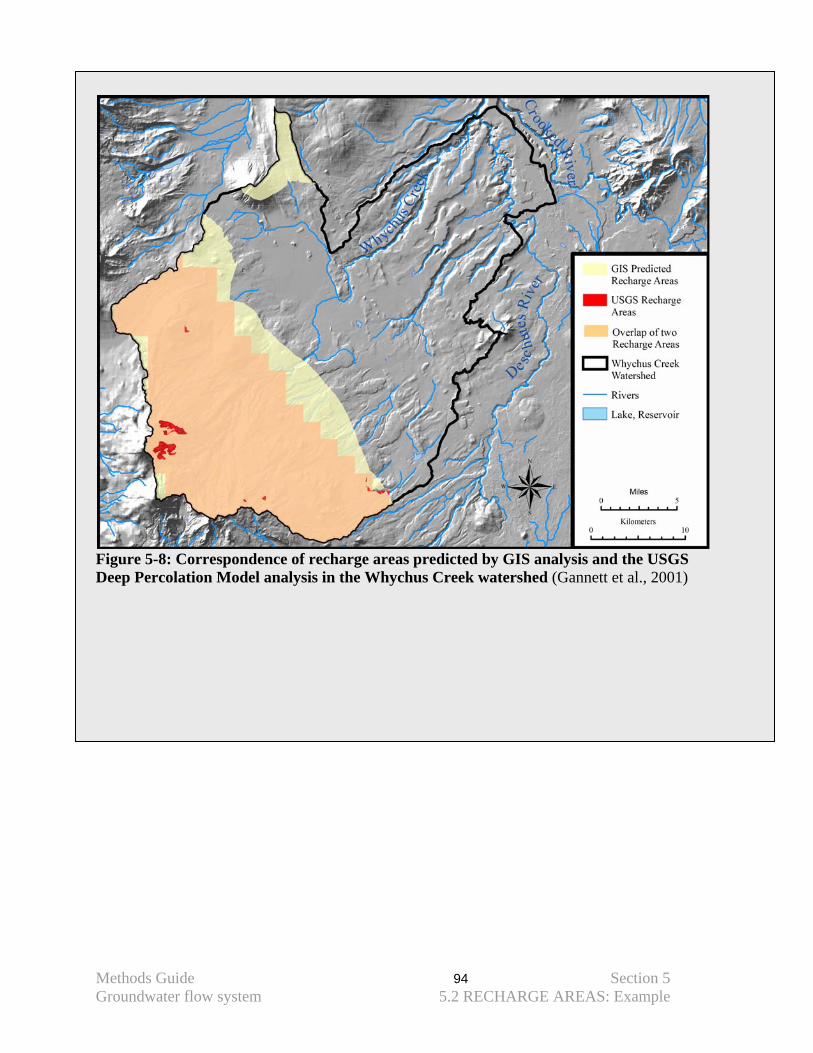
Methods Guide 94 Section 5 Groundwater flow system 5.2 RECHARGE AREAS: Example
Figure 5-8: Correspondence of recharge areas predicted by GIS analysis and the USGS Deep Percolation Model analysis in the Whychus Creek watershed (Gannett et al., 2001)
Methods Guide 95 Section 5 Groundwater flow system 5.2 RECHARGE AREAS: Example
Box 5-1: Incorporating more detailed geologic data, Whychus Creek In the Whychus watershed, we used local geologic information to refine the permeability map produced from the statewide geology data. These refinements were: Glacial Deposits: In the Upper Deschutes subbasin, deposits mapped as glacial deposits (ptype Qg) are generally till (Lite and Gannett, 2002) and would therefore have low permeability. However, glacial deposits west of Sisters are actually outwash (Gannett et al., 2001). Using the guidance in Appendix E, we assigned high permeability to these deposits.
Sedimentary Deposits: We began with the assumption that sedimentary deposits (mapped as Qs) were less permeable. We know that this underestimates the distribution of high permeability material as several more permeable deposits (e.g. alluvium and glacial outwash) are often mapped simply as sedimentary deposits. In several instances we were able to identify some of these sedimentary deposits that are known to be more permeable in this area: • Qal (alluvial deposits) are permeable. Not all alluvium is mapped as such; instead much
of it is mapped as sedimentary (Qs). • Deposits of glacial outwash near La Pine, although mapped as Qs, are quite permeable
(Gannett et al., 2001). • Qf (alluvial fan deposits) are permeable. • Qe (Aeolian deposits) are permeable.
Volcanic Deposits: Quaternary and later Tertiary volcanic deposits have relatively high permeability; older volcanic deposits from the early Tertiary and before tend to have lower permeability. Permeability of volcanic deposits depends on the degree of fracturing; very generally, many of these cracks have been filled in by weathering or secondary mineralization in older volcanic deposits, thus reducing permeability (Gannett et al., 2001). • All volcanic deposits with a map symbol (or ptype) beginning with a ‘Q’ or ‘QT’, for
Quaternary and Quaternary/Tertiary respectively, are classified as more permeable. • All volcanic deposits with a map symbol beginning with a ‘T’ that, according to the
description, occurred in the Pliocene and Miocene epochs are also classified as more permeable.
• The arc-adjacent alluvial plain facies of the Deschutes Formation is sediment interbedded with lava flows and ash-flow tuff and is generally more permeable. These are mapped as Tb, Tp, Ts, and Trd on the geologic map (Lite and Gannett, 2002).
• The proximal lava flows of the Deschutes Formation (or of similar age to this formation) are also generally more permeable. These are mapped as Tb and Tv (Lite and Gannett, 2002).
• The ancestral Deschutes River channel facies of the Deschutes Formation is coarse sand and gravel, distal parts of ash-flow tuffs, and intracanyon lava flows. The coarse grained material and fractured lava flows make it a more permeable deposit (Lite and Gannett, 2002). This area is a portion of that mapped as Tb in the lower Crooked River (Lite and Gannett, 2002).

Methods Guide 96 Section 5 Groundwater flow system 5.2 RECHARGE AREAS: Example
Box 5-1 (continued) • Areas with significantly higher permeability occur in the silicic domes at Cline Buttes
and near Steelhead Falls (Lite and Gannett, 2002). These are mapped as Trd (Lite and Gannett, 2002) and Tca (Walker and MacLeod, 1991).
Methods Guide 97 Section 5 Groundwater Flow Systems Groundwater movement 5.3 Horizontal flow paths
5.3 Groundwater Movement Groundwater movement is complex, and it is often difficult to predict groundwater flow paths. Despite this, it is possible to use simple generalizations to develop an initial hypothesis of the groundwater system at a particular site. To accomplish this, readily available geologic and topographic data can be used to develop conceptual drawings of groundwater flow lines. The depictions of groundwater flow paths can be used to begin identifying areas that are critical for maintaining groundwater quantity and quality. These areas can then be evaluated for existing or proposed activities that could alter the quality or quantity of groundwater as it moves from recharge areas to GDEs. The following section provides guidance on drawing the groundwater flow paths at a conservation area. Groundwater movement is three dimensional, thus drawings of groundwater flow paths will consist of two different components, one depicting the horizontal (or lateral) movement of groundwater and one depicting the vertical movement of groundwater. These initial drawings should be reviewed by a local expert in groundwater hydrology.
5.3.1. Horizontal Flow Paths: Hypothesized horizontal flow paths of groundwater can be represented by drawing arrows on a map of the contributing area. This analysis can be completed using GIS data that has already been gathered in the use of this guidance. It can then be refined through additional information from water table elevations determined from groundwater wells, if these data exist.
Using GIS data:
• Develop a base map: Groundwater flow paths are drawn on a base map of the contributing area. The base map should consist of five sets of information that have already been gathered:
1) Location of GDEs, as mapped in Figure 3-20 2) Contributing area, as mapped in section 5.1 3) Recharge areas, as mapped in section 5.2 4) Topography, as used in section 5.2 5) Surface water bodies – streams, wetlands, and lakes, regardless of their
dependence upon groundwater, as used in Section 3 If this analysis is being done over a very large area that is difficult to represent on one map, consider producing maps for distinct portions of the area.
• Draw hypothesized flow lines:
Draw lines on the base map to represent two sets of groundwater flow paths – regional or intermediate and local (see section 2.5).
i) Regional or intermediate flow lines: These tend to be relatively long flow lines extending from recharge areas to larger springs, larger rivers, or other areas of significant groundwater discharge. To draw these, begin in the recharge areas and draw lines, perpendicular to the elevation contours, toward the points of
Methods Guide 98 Section 5 Groundwater Flow Systems Groundwater movement 5.3 Horizontal flow paths
groundwater discharge (e.g. springs, lakes, gaining reaches of rivers, groundwater-dependent wetlands). Be sure that the lines follow the surface topography downhill and that they begin at higher elevations and end at discharge areas. ii) Local flow lines: These are often relatively short flow lines that extend from high areas that surround or are adjacent to smaller springs, rivers or other areas with smaller groundwater discharge. In general, these flow lines are relatively shallow and as a result should not cross water bodies such as rivers, lakes, or wetlands.
These hypothesized flow lines can be refined using water table elevation data if they exist. See Appendix D for more information on this.
• Have flow paths reviewed by experts
The movement of groundwater can be difficult to predict, in part because our knowledge of underlying geology is incomplete and features such as faults or inclusions can dramatically affect groundwater movement. In addition, there can be local conditions that would cause groundwater to move differently than predicted using these steps. For these reasons, it is important to have the initial prediction of groundwater flow paths reviewed by a local expert in geology, groundwater hydrology, and hydrogeology.
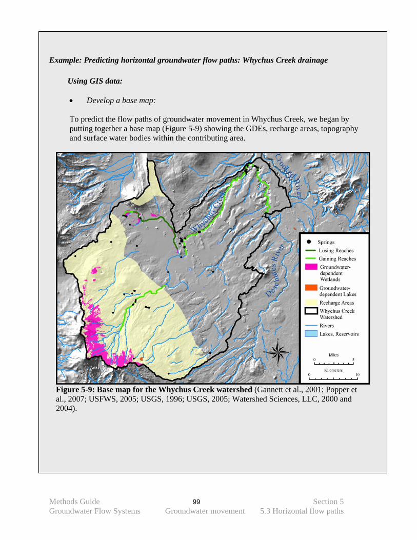
Methods Guide 99 Section 5 Groundwater Flow Systems Groundwater movement 5.3 Horizontal flow paths
Example: Predicting horizontal groundwater flow paths: Whychus Creek drainage
Using GIS data: • Develop a base map: To predict the flow paths of groundwater movement in Whychus Creek, we began by putting together a base map (Figure 5-9) showing the GDEs, recharge areas, topography and surface water bodies within the contributing area.
Figure 5-9: Base map for the Whychus Creek watershed (Gannett et al., 2001; Popper et al., 2007; USFWS, 2005; USGS, 1996; USGS, 2005; Watershed Sciences, LLC, 2000 and 2004).
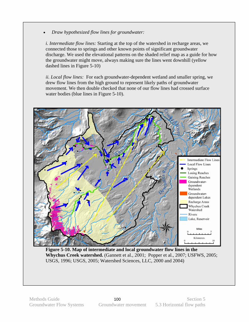
Methods Guide 100 Section 5 Groundwater Flow Systems Groundwater movement 5.3 Horizontal flow paths
• Draw hypothesized flow lines for groundwater: i. Intermediate flow lines: Starting at the top of the watershed in recharge areas, we connected those to springs and other known points of significant groundwater discharge. We used the elevational patterns on the shaded relief map as a guide for how the groundwater might move, always making sure the lines went downhill (yellow dashed lines in Figure 5-10)
ii. Local flow lines: For each groundwater-dependent wetland and smaller spring, we drew flow lines from the high ground to represent likely paths of groundwater movement. We then double checked that none of our flow lines had crossed surface water bodies (blue lines in Figure 5-10).
Figure 5-10. Map of intermediate and local groundwater flow lines in the Whychus Creek watershed. (Gannett et al., 2001; Popper et al., 2007; USFWS, 2005; USGS, 1996; USGS, 2005; Watershed Sciences, LLC, 2000 and 2004)
Methods Guide 101 Section 5 Groundwater Processes Groundwater movement 5.3 Horizontal flow paths
• Have flow paths reviewed by experts:
Our work was reviewed by a local hydrogeologist and modified according to their knowledge of the area. It is important to note that even local experts may not understand the groundwater system with a high degree of certainty unless fairly detailed studies of groundwater have been conducted. However, for the purposes of this effort – to develop an initial focus for conservation action – the local expert probably provides the best available information.
5.3.2. Vertical flow paths: In addition to developing an understanding of how groundwater potentially moves horizontally across the contributing area, it is also important to understand the vertical component of groundwater movement. Knowledge of where groundwater is likely to come from and how deep it is likely to be moving allows for a prediction of which flow paths have the potential to be altered or interrupted by human activities causing impacts to GDEs. Since we cannot easily represent vertical groundwater flow paths throughout the entire contributing area, we construct conceptual drawings along representative transects. This conceptual drawing is called a hydrogeologic cross section. The hydrogeologic cross section illustrates groundwater flow paths below one specific transect in the contributing area. The transect is drawn parallel to the dominant surface water drainage in which the GDEs and species are located. It is selected to provide as much information as possible on the vertical movement of groundwater and the relationship to GDEs. The hydrogeologic cross section is initially constructed using GIS or hard-copy maps that have already been compiled as part of this guidance. It is subsequently refined using water table data, if they exist. Each step in the development of a hydrogeologic cross section is illustrated below using the Whychus Creek example.
Using GIS data:
• Locate the hydrogeologic cross section: Use the same base map you constructed in the previous section (5.3.1). On this map, draw a line to identify the transect under which the hydrogeologic cross section will be developed. In general, this line should be drawn parallel to the dominant surface water drainage in which the groundwater-dependent ecosystems and species are located. However, the location and scale of the cross section should be based on the issue being addressed. For instance, to understand the groundwater inputs to a headwater wetland, the cross section will need to be relatively short and in the upper part of a watershed.
It is possible that not all of the GDEs will be intersected by the transect. This can occur when the biota are located on tributary drainages to the main drainage. If this occurs, it may be necessary to construct additional hydrogeologic cross sections to describe the potential groundwater flow paths supporting these areas.
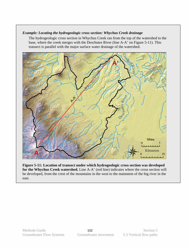
Methods Guide 102 Section 5 Groundwater Flow Systems Groundwater movement 5.3 Vertical flow paths
Example: Locating the hydrogeologic cross section: Whychus Creek drainage The hydrogeologic cross section in Whychus Creek ran from the top of the watershed to the base, where the creek merges with the Deschutes River (line A-A’ on Figure 5-11). This transect is parallel with the major surface water drainage of the watershed.
Figure 5-11: Location of transect under which hydrogeologic cross section was developed for the Whychus Creek watershed. Line A-A’ (red line) indicates where the cross section will be developed, from the crest of the mountains in the west to the mainstem of the big river in the east.
A
A’
Methods Guide 103 Section 5 Groundwater Flow Systems Groundwater movement 5.3 Vertical flow paths
• Gather the data to construct the hydrogeologic cross section Five sets of data are used to develop the hydrogeologic cross section below this transect: 1. A topographic map Either electronic or hard copy, in which elevational gradients across a fairly broad area are visible. A 1:24000 map or 10 m DEM is best, especially if the topography is more subdued. 2. A surficial geology map Again, either electronic or hard copy. Use the best or most detailed data available. 3. Information on the depths of geologic deposits This is sometimes the most difficult to find but it is useful. Often there are three dimensional diagrams of geologic substrate that have been put together by the USGS. Potential sources of information are:
* Hydrologic Atlas http://capp.water.usgs.gov/gwa/ch_h/index.html * Well log records, available in Washington at http://apps.ecy.wa.gov/welllog/
and in Oregon at http://apps2.wrd.state.or.us/apps/gw/well_log/Default.aspx * USGS reports on specific areas. Check the USGS publication warehouse for
studies related to a particular area at http://infotrek.er.usgs.gov/pubs/ 4. Location of groundwater discharge areas This is any groundwater dependent lake, wetland and river as well as all springs, as identified in section 3. 5. Location of groundwater recharge areas As developed in section 5.2.
Example: Gather data to construct hydrogeologic cross section: Whychus Creek drainage We located the five sets of data from the following sources: 1. A topographic map – We used the topographic map from the Oregon Gazeteer. 2. A geologic map – We used the surficial geology mapped developed for the
identification of recharge areas (section 5.2). 3. Information on the depths of geologic deposits – We obtained this information from a
USGS publication describing the groundwater system of the Upper Deschutes Basin (Gannett et al., 2001).
4. Location of groundwater discharge areas – This was mapped as part of the analysis in section 3 (Figure 3-20).
5. Location of groundwater recharge areas – This was mapped earlier in this section (5.2, Figure 5-8).
Methods Guide 104 Section 5 Groundwater Flow Systems Groundwater movement 5.3 Vertical flow paths
• Draw the outline of the hydrogeologic cross section:
The hydrogeologic cross section is drawn on a blank piece of paper, either by hand or electronically using drawing software. ArcGIS has an automated procedure for doing this. If completing this by hand, begin by constructing an outline of the cross-sectional area by drawing a y- and an x-axis, much as one would when constructing a graph; these will form the left and bottom sides of the cross-sectional area. The y-axis is elevation, starting from the ground surface elevation at the highest point along the transect (top of graph), and ending at the lowest elevation along the transect (bottom of graph). The x-axis is the distance from the high point to the lowest point on the transect. Both axes should be drawn to scale, although their individual scales may differ from each other; for instance the y-axis scale may be in meters to represent depth below the ground surface, while the x-axis scale may be in kilometers, to represent distance along the ground.
After drawing the x- and y-axes, draw the longitudinal profile of the land surface, which is a line illustrating the topographic patterns of the land surface, beginning at the highest elevation on the transect and ending at the lowest elevation. Use the topographic map to approximate the surface elevation patterns, following the scales established by the y- and x-axes that have already been drawn.
Finally, draw a straight line that connects the lowest point along the longitudinal profile with the x-axis. The final product should be a square in which the left, bottom and right sides are straight while the top side is uneven and illustrates the topographic patterns of the land surface.
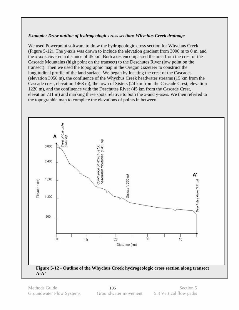
Methods Guide 105 Section 5 Groundwater Flow Systems Groundwater movement 5.3 Vertical flow paths
Example: Draw outline of hydrogeologic cross section: Whychus Creek drainage
We used Powerpoint software to draw the hydrogeologic cross section for Whychus Creek (Figure 5-12). The y-axis was drawn to include the elevation gradient from 3000 m to 0 m, and the x-axis covered a distance of 45 km. Both axes encompassed the area from the crest of the Cascade Mountains (high point on the transect) to the Deschutes River (low point on the transect). Then we used the topographic map in the Oregon Gazeteer to construct the longitudinal profile of the land surface. We began by locating the crest of the Cascades (elevation 3050 m), the confluence of the Whychus Creek headwater streams (15 km from the Cascade crest, elevation 1463 m), the town of Sisters (24 km from the Cascade Crest, elevation 1220 m), and the confluence with the Deschutes River (45 km from the Cascade Crest, elevation 731 m) and marking these spots relative to both the x-and y-axes. We then referred to the topographic map to complete the elevations of points in between.
Figure 5-12 - Outline of the Whychus Creek hydrogeologic cross section along transect A-A’
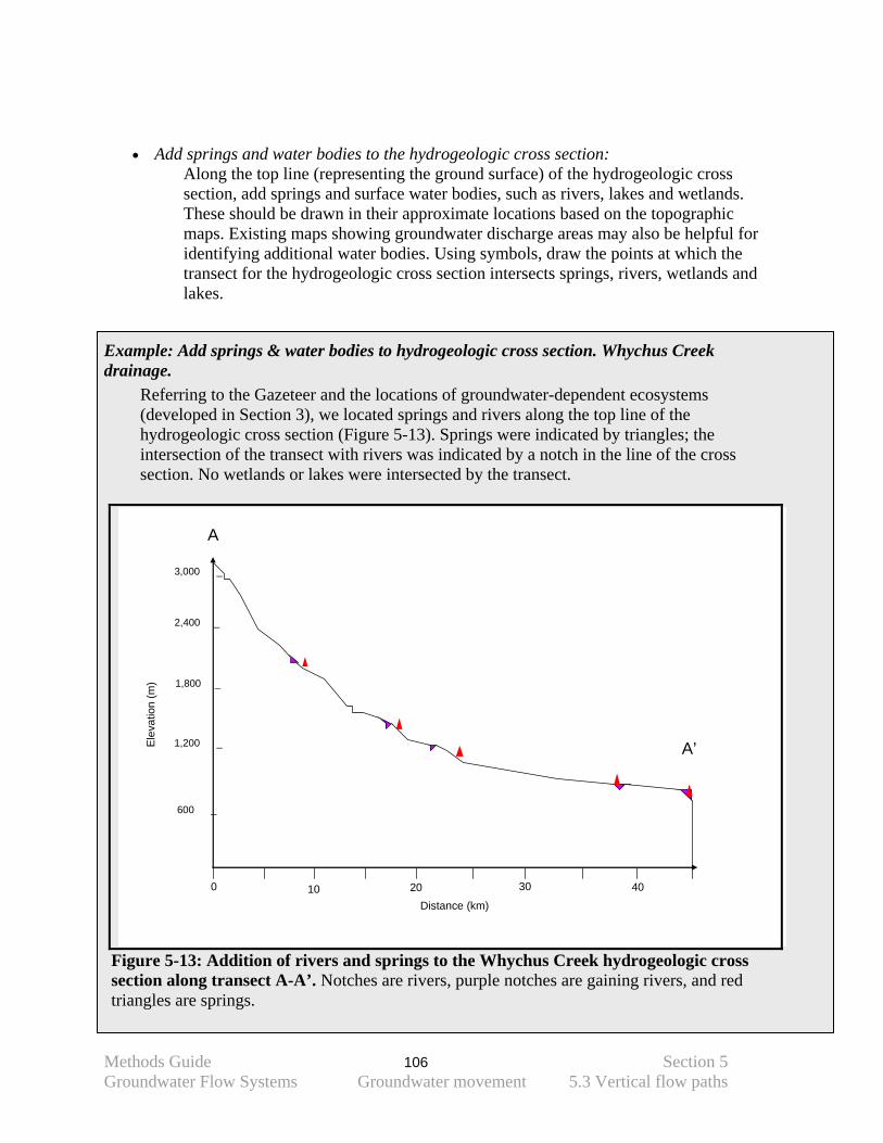
Methods Guide 106 Section 5 Groundwater Flow Systems Groundwater movement 5.3 Vertical flow paths
• Add springs and water bodies to the hydrogeologic cross section:
Along the top line (representing the ground surface) of the hydrogeologic cross section, add springs and surface water bodies, such as rivers, lakes and wetlands. These should be drawn in their approximate locations based on the topographic maps. Existing maps showing groundwater discharge areas may also be helpful for identifying additional water bodies. Using symbols, draw the points at which the transect for the hydrogeologic cross section intersects springs, rivers, wetlands and lakes.
Example: Add springs & water bodies to hydrogeologic cross section. Whychus Creek drainage.
Referring to the Gazeteer and the locations of groundwater-dependent ecosystems (developed in Section 3), we located springs and rivers along the top line of the hydrogeologic cross section (Figure 5-13). Springs were indicated by triangles; the intersection of the transect with rivers was indicated by a notch in the line of the cross section. No wetlands or lakes were intersected by the transect.
3,000 _
2,400 _
1,800 _
1,200 _
600 _
Distance (km)
Elev
atio
n (m
)
300 4010 20
A
A’
Figure 5-13: Addition of rivers and springs to the Whychus Creek hydrogeologic cross section along transect A-A’. Notches are rivers, purple notches are gaining rivers, and red triangles are springs.
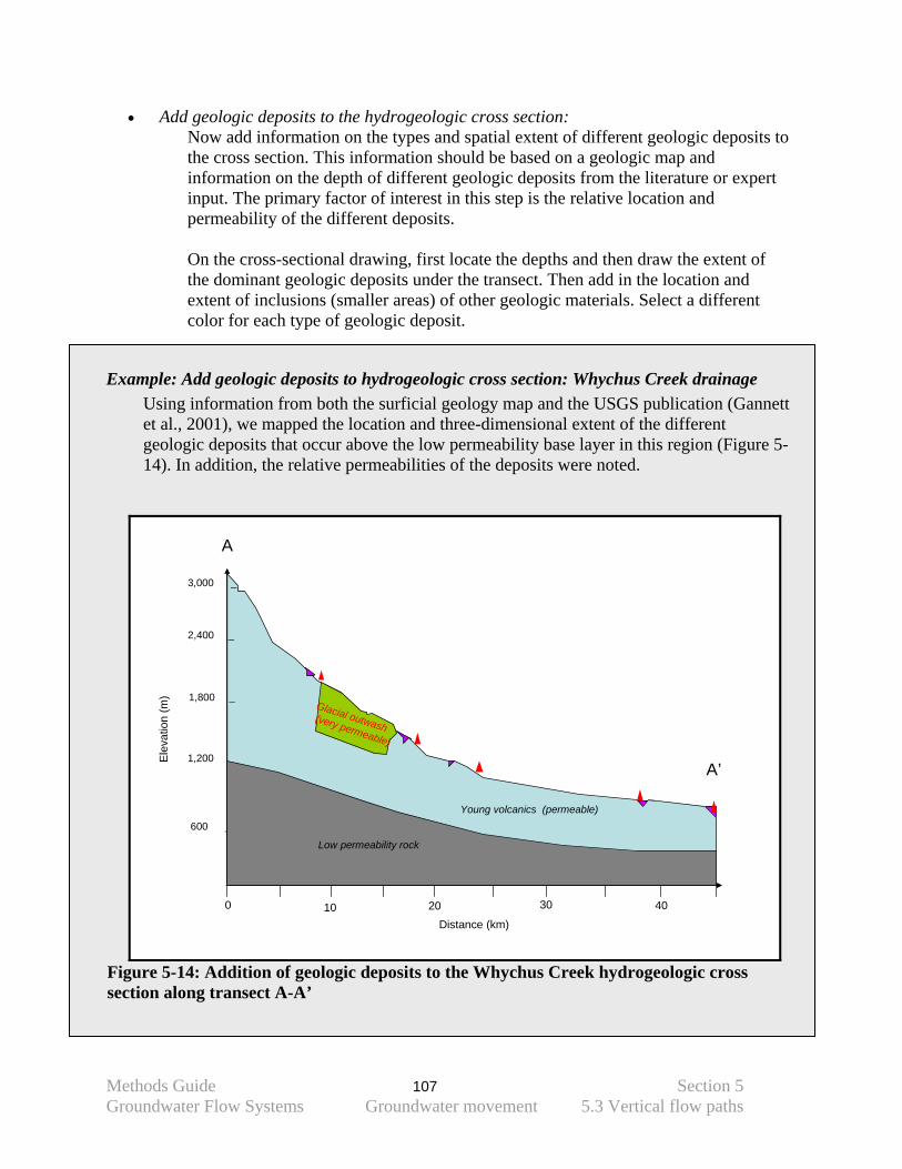
Methods Guide 107 Section 5 Groundwater Flow Systems Groundwater movement 5.3 Vertical flow paths
• Add geologic deposits to the hydrogeologic cross section: Now add information on the types and spatial extent of different geologic deposits to the cross section. This information should be based on a geologic map and information on the depth of different geologic deposits from the literature or expert input. The primary factor of interest in this step is the relative location and permeability of the different deposits.
On the cross-sectional drawing, first locate the depths and then draw the extent of the dominant geologic deposits under the transect. Then add in the location and extent of inclusions (smaller areas) of other geologic materials. Select a different color for each type of geologic deposit.
Example: Add geologic deposits to hydrogeologic cross section: Whychus Creek drainage Using information from both the surficial geology map and the USGS publication (Gannett et al., 2001), we mapped the location and three-dimensional extent of the different geologic deposits that occur above the low permeability base layer in this region (Figure 5-14). In addition, the relative permeabilities of the deposits were noted.
3,000 _
2,400 _
1,800 _
1,200 _
600 _
Low permeability rock
Distance (km)
Glacial outwash(very permeable)
Young volcanics (permeable)
Elev
atio
n (m
)
300 4010 20
A
A’
Figure 5-14: Addition of geologic deposits to the Whychus Creek hydrogeologic cross section along transect A-A’
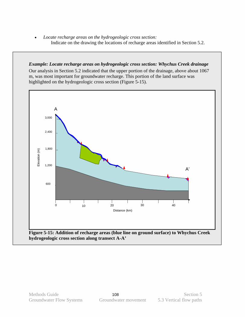
Methods Guide 108 Section 5 Groundwater Flow Systems Groundwater movement 5.3 Vertical flow paths
• Locate recharge areas on the hydrogeologic cross section:
Indicate on the drawing the locations of recharge areas identified in Section 5.2.
Example: Locate recharge areas on hydrogeologic cross section: Whychus Creek drainage Our analysis in Section 5.2 indicated that the upper portion of the drainage, above about 1067 m, was most important for groundwater recharge. This portion of the land surface was highlighted on the hydrogeologic cross section (Figure 5-15).
3,000 _
2,400 _
1,800 _
1,200 _
600 _
Distance (km)
Ele
vatio
n (m
)
300 4010 20
A
A’
Figure 5-15: Addition of recharge areas (blue line on ground surface) to Whychus Creek hydrogeologic cross section along transect A-A’
Methods Guide 109 Section 5 Groundwater Flow Systems Groundwater movement 5.3 Vertical flow paths
• Draw hypothesized vertical flow lines on the hydrogeologic cross section:
Draw lines on the hydrogeologic cross section to represent possible or hypothesized groundwater flow paths. As discussed for the horizontal flow lines, we suggest drawing regional or intermediate flow lines first, followed by local flow lines. Drawing all lines is an iterative process based on the steps provided below. Begin with the first step and draw some initial lines. Then move onto the second step and adjust or modify the lines as needed. Continue in this way through all of the steps then return to the first step to confirm that the flow lines are consistent with the guidance provided in each step.
A. Draw the regional or intermediate flow lines on the hydrogeologic cross section:
i. Connect recharge to discharge areas: Begin in the recharge areas and draw lines towards the points of groundwater discharge (e.g. springs, lakes, gaining reaches of rivers, groundwater dependent wetlands). Be sure that the lines follow the surface topography downhill.
ii. Adjust flow lines to the permeability of geologic deposits: Lateral groundwater flow paths generally occur in more permeable deposits. If the flow lines intersect a less permeable layer, they will steepen (be more vertical); if the flow lines go through a more permeable deposit, they will flatten out.
B. Draw the local flow lines:
i. Connect high areas adjacent to water bodies or springs with points of groundwater discharge.
ii. Adjust flow lines so they do not cross surface water bodies: Groundwater flow paths that are near the surface cannot cross surface water bodies such as lakes, streams or wetlands.
• Have flow paths reviewed by experts
As discussed earlier, it is it is important to have the initial prediction of vertical groundwater flow paths reviewed by a local expert in geology or hydrogeology.
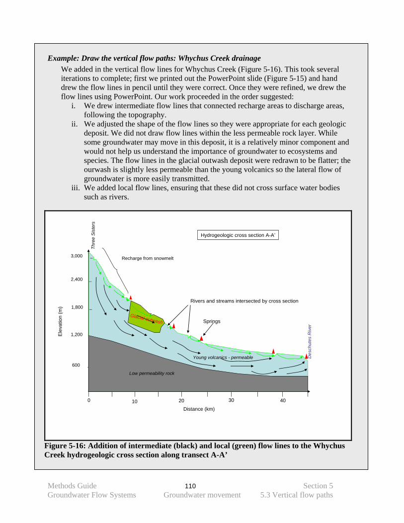
Methods Guide 110 Section 5 Groundwater Flow Systems Groundwater movement 5.3 Vertical flow paths
Example: Draw the vertical flow paths: Whychus Creek drainage We added in the vertical flow lines for Whychus Creek (Figure 5-16). This took several iterations to complete; first we printed out the PowerPoint slide (Figure 5-15) and hand drew the flow lines in pencil until they were correct. Once they were refined, we drew the flow lines using PowerPoint. Our work proceeded in the order suggested:
i. We drew intermediate flow lines that connected recharge areas to discharge areas, following the topography.
ii. We adjusted the shape of the flow lines so they were appropriate for each geologic deposit. We did not draw flow lines within the less permeable rock layer. While some groundwater may move in this deposit, it is a relatively minor component and would not help us understand the importance of groundwater to ecosystems and species. The flow lines in the glacial outwash deposit were redrawn to be flatter; the ourwash is slightly less permeable than the young volcanics so the lateral flow of groundwater is more easily transmitted.
iii. We added local flow lines, ensuring that these did not cross surface water bodies such as rivers.
3,000 _
2,400 _
1,800 _
1,200 _
600 _
Des
chut
es R
iver
Low permeability rock
Distance (km)
Thre
e S
iste
rs
Glacial outwash
Young volcanics - permeable
Recharge from snowmelt
Hydrogeologic cross section A-A’
Ele
vatio
n (m
)
Rivers and streams intersected by cross section
Springs
300 4010 20
Figure 5-16: Addition of intermediate (black) and local (green) flow lines to the Whychus Creek hydrogeologic cross section along transect A-A’

Methods Guide 111 Section 5 Groundwater Flow Systems Groundwater movement 5.3 Vertical flow paths
Finally, we had Figure 5-16 reviewed by a geologist who checked the location, extent and permeability assignments of the geologic deposits as well as the hypothesized flow lines.
Methods Guide 112 Section 6 Groundwater Flow System 6.0 Summary
6. SUMMARY This methods guide provides guidance on identifying groundwater-dependent biodiversity, developing an understanding of how these ecosystems and species depend on groundwater, identifying the key ecological attributes that should be the focus of conservation strategies, and producing an initial conceptual model of the groundwater flow system at a particular site. All of these products set the stage for the next step in conservation planning – identification of threats and then design of conservation strategies to abate those threats. As a result of using the methods guide, a site manager should know:
1) the ecosystems and species that depend on groundwater and where they are located 2) the ecological attributes that are essential to maintain GDEs and the desired future
conditions of these attributes that will further the integrity of the ecosystems and species 3) how groundwater is likely to reach GDEs and therefore the places on the landscape where groundwater extraction or contamination pose a threat to the conservation of GDEs.
The major caveat: Products should be reviewed by technical experts All products from this work – identification of GDEs, groundwater requirements of GDEs, the hypothesized recharge areas, and conceptual models of vertical and horizontal flow paths – should be reviewed by experts familiar with the ecology, hydrogeology, geology or hydrology of the area. The methods described here are based on generalizations, such as the relationship of groundwater flow patterns to surficial geology and topography. Invariably, there are local exceptions to these rules so it is important to get review of interim and final products. In some cases additional analysis by technical experts will be needed. The work completed through the Methods Guide will serve as a starting point for discussions with experts, who can then focus on refining the existing work rather than developing initial assessments. In addition, the products from the Methods Guide can be used to more narrowly identify uncertainties that are critical to conservation and that may need to be addressed with further study. The next step of conservation planning: The information generated through the Methods Guide sets the stage for identifying land- and water-use activities that are likely to threaten the groundwater supply to GDEs. Groundwater extraction activities in the hypothesized flow paths should be evaluated further to determine their potential to reduce groundwater availability for GDEs. Land-use activities located in recharge areas should be further evaluated for their potential to contaminate the groundwater supplying GDEs. Finally, monitoring should be initiated that will assess whether the measurable objectives identified for each GDE are met.
Methods Guide 113 References
REFERENCES
Aldous, A. 2007. The Nature Conservancy. Unpublished data. Alley, W.M. and S.A. Leake. 2004. The journey from safe yield to sustainability. Ground Water.
42(1):12-16. Almendinger, J.E. and J.H. Leete. 1998a. Regional and local hydrogeology of calcareous fens in
the Minnesota River basin, USA. Wetlands 18(2): 184-202. Almendinger, J.E. and J. H. Leete. 1998b. Peat characteristics and groundwater geochemistry of
calcareous fens in the Minnesota River Basin, U.S.A. Biogeochemistry 43(1):17-41. Andelman, S., K. Gillem, C. Groves, C. Hansen, J. Humke, T. Klahr, L. Kramme, B. Moseley,
M. Reid, D. Vander Schaaf, M. Coad, C. DeForest, C. MacDonald, J. Baumgartner, J. Hak, S. Hobbs, L. Lunte, L. Smith, and C. Soper. 1999. The Columbia Plateau Ecoregional Assessment: a pilot effort in Ecological Conservation. The Nature Conservancy. 71 electronic pages. Available at: http://conserveonline.org/coldocs/2006/01/Columbia%20Plateau%20Final%20Assessment.pdf
Bauer, H.H. and J.J. Vaccaro. 1987. Documentation of a deep percolation model for estimating
ground-water recharge. USGS Open-File Report 86-536. 180 pp. Availabe at: http://pubs.er.usgs.gov/usgspubs/ofr/ofr86536
Bedford, B.L. 1999. Cumulative effects on wetland landscapes: links to wetland restoration in
the United States and southern Canada. Wetlands 19(4): 775-788. Bedford, B.L. and K.S. Godwin. 2003. Fens of the United States: Distribution, Characteristics,
and Scientific Connection Versus Legal Isolation. Wetlands 23(3):608-629. Bell-McKinnon, M. 2002. Water Quality Assessments of Volunteer Monitored Lakes within
Washington State 1998-1999. Washington State Department of Ecology Publication No. 02-03-019. 35 pp. Available at: http://www.ecy.wa.gov/biblio/0203019.html
Breitbart, M., S. Leeds, T. Schoenfeld, and F. Rohwer. 2004. Phage community dynamics in hot
springs. Applied and Environmental Microbiology 70(3): 1633-1640. Brinson, M. M. 1993. A Hydrogeomorphic Classification for Wetlands. U.S. Army Corps of
Engineers Waterways Experiment Station, Vicksburg, MS. Brooks, J.R., F.C. Meinzer, R. Coulombe, and J. Gregg. 2002. Hydraulic redistribution of soil
water during summer drought in two contrasting Pacific Northwest coniferous forests. Tree Physiology 22:1107-1117.
Methods Guide 114 References
Brown, J., L. Bach, A. Aldous, and A. Wyers. 2007. Overcoming data shortfalls to locate groundwater-dependent ecosystems and assess threats to groundwater quantity and quality. In: L. Ribiero, A. Chambel, and M.T. Condesso de Melo (Eds). Proceedings of the XXXV IAH Congress International Association of Hydrogeologists Groundwater and Ecosystems. Lisbon, September 17-21, 2007. Paper # 461.
Brunke, M. and T. Grosner. 1997. The ecological significance of exchange processes between
rivers and groundwater. Freshwater Biology 37: 1–33. Buchanan, David, Mary L. Hanson, Robert M. Hooton - Oregon Department of Fish & Wildlife.
1997. Status Of Oregon's Bull Trout, Distribution, Life History, Limiting Factors, Management Considerations, and Status, 1997 Technical Report. Report to Bonneville Power Administration, Contract No. 1994BI34342, Project No. 199505400, 185 electronic pages (BPA Report DOE/BP-34342-5). Available at: http://www.efw.bpa.gov/Publications//R34342-5.pdf
Busch, D.E., N.L. Ingraham, and S.D. Smith. 1992. Water uptake in woody riparian
phreatophytes of the southwestern United States: A stable isotope study. Ecological Applications 2(4):450-459.
Cairns Jr., J., P.V. McCormick, and B.R. Niederlehner. 1993. A proposed framework for
developing indicators of ecosystem health. Hydrobiologia 263(1):1-44. Caldwell, M.M., T.E. Dawson, and J.H. Richards. 1998. Hydraulic lift: consequences of water
efflux from the roots of plants. Oecologia 113:151-161. Carlson, R.E. 1977. A Trophic State Index for Lakes. Limnology and Oceanography 22:361-369. Carlton, J. 2006. Cities spend millions on land to protect water. Wall Street Journal. January 4,
2006. P. B-6. Carter,V. 1996. Technical Aspects of Wetlands: Wetland hydrology, water quality and
associated functions. In: USGS. National Water Summary on Wetland Resources. USGS Water-Supply Paper 2425. Pp. 35-48.
Christy, J. 2004. Native Freshwater Plant Associations of Northwestern Oregon. Oregon Natural
Heritage Information Center, Oregon State University. 246 pp. Available at: http://oregonstate.edu/ornhic/christy2004.pdf
Ciruna, K. and A. Aldous. 2005. Appendix A: Ecological characteristics of freshwater ecosystem
type. In: N. Silk and K. Ciruna (Eds) A practitioner’s guide to freshwater biodiversity conservation. Washington D.C.: Island Press. Pp.341-366.
Columbia River Inter-Tribal Fish Commission (CRITFC). 2004. Reach_QHA geographic data.
Available at: ftp://ftp.streamnet.org/toast/data/deschutes.
Methods Guide 115 References
Daly, C. and G. Taylor. 1998. Oregon Average Monthly or Annual Precipitation, 1961-90. Water and Climate Center of the Natural Resources Conservation Service. Available at: http://www.ocs.orst.edu/prism/.
Dawson, T.E. and Ehleringer, J.R. 1991. Streamside trees that do not use stream water. Nature
350: 335-337. DeJong, G.D., S.P. Canton, and J.W. Chadwick. 2005. Macroinvertebrates occurring in Sunbeam
Hot Springs, an absolutely hot spring in Idaho, USA. Journal of Freshwater Ecology. 20(3):611-613.
Dunne, T. and L.B. Leopold. 1978. Water in Environmental Planning. New York: W.H.
Freeman and Company. 818 pp. Eamus, D. and R. Froend. 2006. Groundwater-dependent ecosystems: the where, what and why
of GDEs. Australian Journal of Botany 54:91-96. Eamus, D., R. Froend, R. Loomes, G. Hose, and B. Murray. 2006. A functional methodology for
determining the groundwater regime needed to maintain the health of groundwater-dependent vegetation. Australian Journal of Botany. 54:97-114.
Erman, N.A. and D.C. Erman. 1995. Species permanence, Trichoptera species richness and the
role of drought. Journal of the Kansas Entomological Society 68(2) supplement: 50-64. Evans, W.C., R.H. Mariner, S.E. Ingebritsen, B.M. Kennedy, M.C. van Soest, and M.A.
Huebner. 2002. Report of hydrologic investigations in the Three Sisters area of central Oregon, summer 2001. US Geological Survey Water-Resources Investigations Report 02-4061. 13 pp.
Frest, T. J. and E.J. Johannes. 1995. Interior Columbia Basin mollusk species of special concern.
Final Report to Interior Columbia Basin Ecosystem Management Project. 286 pp. Froend, R. and R. Loomes. 2004. Approach to determination of ecological water requirements of
groundwater dependent ecosystems in Western Australia. A report to the Department of the Environment. 83 electronic pages.
Galas, J. 2005. Human impact on physical and chemical properties of springs from Cracow-
Czestochowa Upland (southern Poland). Polish Journal of Ecology 53(3):329-341 Gannett, M.W., K.E. Lite Jr., D.S. Morgan, and C.A. Collins. 2001. Ground-water hydrology of
the Upper Deschutes Basin, Oregon. USGS Water-Resources Investigations Report 00-4162. 77 pp.
Gannett, M.W., K. E. Lite Jr., J. L. La Marche, B. J. Fisher, and D. J. Polette. 2007. Ground-
Water Hydrology of the Upper Klamath Basin, Oregon and California. USGS Scientific Investigations Report 2007–5050. 98 electronic pages.
Methods Guide 116 References
Gordon, N.D., T.A. McMahon, and B.L. Finlayson. 1993. Stream Hydrology: An Introduction
for Ecologists. Chichester: John Wiley and Sons. 526 pp. Groves, C.R. 2003. Drafting a Conservation Blueprint: A Practitioner’s guide to Planning for
Biodiversity. Washington DC: Island Press. Groves, C., L. Valutis, D. Vosick, B. Neely, K. Wheaton, J. Touval, and B. Runnels. 2000.
Designing a Geography of Hope Volume 1. April 2000. 85 pp. Groundwater Protection Council (GWPC). 2007. Accessed website November 16, 2007:
http://www.gwpc.org/e-library/e-library_documents/e- library_documents_state_fact_sheets/washington.pdf
Hacke, U.G., J. S. Sperry, and J. Pittermann. 2000. Drought experience and cavitation resistance
in six shrubs from the Great Basin, Utah. Basic and Applied Ecology. 1:31-41. Hogg, I.D. and D.D. Williams. 1996. Response of stream invertebrates to a global warming
thermal regime: an ecosystem-level manipulation. Ecology 77:395-407. Hultine, K.R., R. L. Scott, W. L. Cable, D. C. Goodrich, and D. G. Williams. 2004. Hydraulic
redistribution by a dominant, warm-desert phreatophyte: seasonal patterns and response to precipitation pulses. Functional Ecology 18:530-538.
Ingebritsen, S.E., D.R. Sherrod, and R.H. Mariner. 1989. Heat flow and hydrothermal circulation
in the Cascade Range, North-Central Oregon. In: Proceedings of Workshop XLIV Geological, Geophysical, and Tectonic Setting of the cascade Range. USGS Geothermal Research Program Open File Report 89-178.
Ingebritsen, S.E., R.H. Mariner, and D.R. Sherrod. 1994. Hydrothermal systems of the Cascade
Range, North-Central Oregon. USGS Professional Paper 1044-L. Jackson, R.B., J. Canadell, J.R. Ehleringer, H.A. Mooney, O.E. Sala, and E.D. Schulze. 1996. A
global analysis of root distributions for terrestrial biomes. Oecologia 108:389-411. Jackson, R.B., J.S. Sperry, and T.E. Dawson. 2000. Root water uptake and transport: using
physiological processes in global predictions. Trends in Plant Science. 5(11):482-488. Jefferson, A. and G. Grant. 2005. Groundwater systems of the McKenzie River watershed,
Oregon High Cascades. Presentation at Under the Pacific Northwest: Integrating research, policy and education. November 2-3, 2005, Stevenson, WA.
Jefferson, A., G. Grant, and T. Rose. 2006. The influence of volcanic history on groundwater
patterns on the west slope of the Oregon High Cascades. Water Resources Research 42, W12411, doi:10.1029/2005WR004812.
Methods Guide 117 References
Jones, J.L. and R.J. Wagner. 1995. Water-quality assessment of the central Columbia Plateau in Washington and Idaho; analysis of available nutrient and pesticide data for ground water, 1942-92. USGS Water-Resources Investigations Report 94-4258. 119 pp. Available at: http://pubs.er.usgs.gov/usgspubs/wri/wri944258
Kernohan, B.J. and J.B. Haufler. 1999.Implementation of an effective process for the
conservation of biological diversity. In: Baydock,R.K., H.Campa III, and J.B. Haufler (Eds). Practical Approaches to the Conservation of Biological Diversity. Washington D.C.: Island Press. Pp. 233-249.
King County Department of Natural Resources. 2000. Literature Review and Recommended
Sampling Protocol for Bull Trout in King County. Seattle, WA. June 2000. Available at: http://dnr.metrokc.gov/stock/pdf/docs/wlr/BullTrtWhtPP/BullTrWP.pdf
Komor, S.C. 1994. Geochemistry and hydrology of a calcareous fen within the Savage fen
wetlands complex, Minnesota, U.S.A. Geochimica et Cosmochimica Acta 58: 3353-3367 Kudray, G.M. and M.R. Gale. 2000. Evaluation of National Wetlands Inventory maps in a
heavily forested region of the Upper Great Lakes. Wetlands 20(4): 581-587. Kulzer, L., S. Luchessa, S. Cooke, R. Errington and F. Weinmann. 2001. Characteristics of low
elevation Sphagnum dominated peatlands of western Washington: A Community Profile. Part 1: Physical, chemical, and vegetation characteristics. King County Water and Land Division Publication. 15 pp. Available at: http://dnr.metrokc.gov/wlr/dss/sphagnum-bogs.htm
Kuzila, M.S., D.C. Rundquist, and J.A. Green. 1991. Models for estimating wetland loss: The
Rain Basin Region of Nebraska, 1927-1981. Journal of Soil and Water Conservation 46(6):441-446.
LaMarche, Jonathan. 2006. Oregon Water Resources Department. Personal communication. Lee, B.D., R. C. Graham, T. E. Laurent, C. Amrhein, and R. M. Creasy. 2001. Spatial
Distributions of Soil Chemical Conditions in a Serpentinitic Wetland and Surrounding Landscape. Soil Science Society of America Journal 65:1183–1196.
Lee, D.R. 1977. A device for measuring seepage flux in lakes and estuaries. Limnology and
Oceanography 22(1):140-147. Lee, K.K. and Risley, J.C. 2002. Estimates of ground-water recharge, base flow, and stream
reach gains and losses in the Willamette River Basin, Oregon. U.S. Geological Survey Water-Resources Investigations Report 01–4215. 52 p.
LeMaitre, D.C., D.F. Scott, and C. Colvin. 1999. A review of information on interactions
between vegetation and groundwater. Water South Africa (SA) 25(2): 137- 152.
Methods Guide 118 References
Lite Jr., K.E. and M.W. Gannett. 2002. Geologic framework of the regional ground-water flow system in the Upper Deschutes Basin, Oregon. USGS Water-Resources Investigations Report 02-4015. 44 pp.
Lodge, D.M., D.P. Krabbenhoft, and R.G. Striegl. 1989. A positive relationship between
groundwater velocity and submersed macrophyte biomass in Sparkling Lake, Wisconsin. Limnology and Oceanography. 34(1): 235-239.
Lower Columbia Fish Recovery Board. 2004. Lower Columbia Salmon Recovery and Fish &
Wildlife Subbasin Plan: Appendix B Chapter 19 Band Tailed Pigeon. 4pp. Available at: http://www.lcfrb.gen.wa.us/December%20Final%20%20Plans/lower_columbia_salmon_recovery_a.htm
Manga, M. 1996. Hydrology of spring-dominated streams in the Oregon Cascades. Water
Resources Research 32(8):2435-2439. Manga, M. 2001. Using springs to study groundwater flow and active geologic processes.
Annual Review of Earth Planetary Sciences 29:201-228. Margules, C.R. and R.L. Pressey. 2000. Systematic conservation planning. Nature. 405:243-253. Naiman, R.J., H. Decamps, and M.E. McClain. 2006. Riparia: Ecology, Conservation, and
Management of Streamside Communities. Burlington: Elsevier Academic Press. Naumberg, E., R. Mata-gonzalez, R.G. Hunter, T. McIendon, and D.W. Martin. 2005.
Phreatophytic vegetation and groundwater fluctuations: A review of current research and application of ecosystem response modeling with an emphasis on Great Basin vegetation. Environmental Management 35(6): 726-740.
North West Habitat Institute (NWHI). 2002. US Columbia River Basin Current Wildlife-Habitat
Types (grouped into categories by The Nature Conservancy). Available at: http://www.nwhi.org.
Northwest Power and Conservation Council. Downloaded December, 2005. Appendix I. Focal
Fish Characterization. In: Northwest Power and Conservation Council. Deschutes Subbasin Plan. Portland, Oregon. Available at: http://www.nwcouncil.org/fw/subbasinplanning/deschutes/plan/
O’Grady, A.P., D. Eamus, P.G. Cook, and S. Lamontagne. 2006. Groundwater use by riparian
vegetation in the wet-dry tropics of northern Australia. Australian Journal of Botany 54:145-154.
Oregon Department of Environmental Quality. 2003. 2003 Oregon Groundwater Conditions.
Available at: http://www.deq.state.or.us/wq/groundwater/docs/orgwconds.pdf
Methods Guide 119 References
Oregon Office of Economic Analysis. 2007. http://www.oea.das.state.or.us/DAS/OEA/demographic.shtml Cited Jan. 8, 2007
Oregon Water Resources Department. 2007.
http://egov.oregon.gov/OWRD/PUBS/aquabook_protections.shtml Cited November 17, 2007
Oregon Water Resources Department Strategic Outlook. 2007.
http://www.oea.das.state.or.us/DAS/OEA/demographic.shtml . Cited June 15, 2007 Pacific Northwest Hydrography Framework (PNWHF). 2005. Water bodies, Water courses,
water points. Vector digital data. Portland, OR. OR BLM. http://www.oregon.gov/DAS/EISPD/GEO/alphalist.shtml#H
Parrish, J.D., D.P. Braun, and R.S. Unnasch. 2003. Are we conserving what we say we are?
Measuring ecological integrity within protected areas. Bioscience. 53(9): 851-860. Poole, G.C. and C.H. Berman. In press. Pathways of human influence on water temperature
dynamics in stream channels. Environmental Management. Popper, K., G. Wilhere, M. Schindel, D. VanderSchaaf, P. Skidmore, G. Stroud, J. Crandall, J.
Kagan, R. Crawford, G. Kittel, J. Azerrad, and L. Bach. 2007. The East Cascades - Modoc Plateau and West Cascades Ecoregional Assessments. Prepared by The Nature Conservancy and the Washington Department of Fish and Wildlife with support from the Oregon Natural Heritage Information Center, Washington Heritage Program, and Natureserve. The Nature Conservancy, Portland, Oregon. 368 electronic pages. Available at: http://conserveonline.org/coldocs/2007/08/EW_Cascades_EA_Oregon_Portfolio_Site_Summaries_COL.pdf
Power, G., R.S. Brown, and J.G. Imhof. 1999. Groundwater and fish- insights from northern
North America. Hydrological Processes 13:401-422. Raymond Jr., L.S. What is Groundwater? University of Minnesota Extension Service Bulletin.
http://www.extension.umn.edu/distribution/naturalresources/DD5867.html Riehle, M.D. and J. Lovtang. 2000. Squaw Creek Education and Restoration Project 1998-1999.
Report for Deschutes National Forest. 39 pp. Riggs, G.B. 1958. Peat resources of Washington. Washington State Division of Mines and
Geology Bulletin No. 44. 272 pp. Rosenberry, D.O., R.G. Striegl, and D.C. Hudson. 2000. Plants as indicators of focused ground
water discharge to a northern Minnesota Lake. Ground Water 38(2):296-303.
Methods Guide 120 References
Sada, D.W. Unpublished 2005. DRAFT: A conceptual model describing general biotic/hydrologic/ human activity relationships in arid land springs systems.
Sada, D.W and K.F. Pohlmann. 2006. Draft U.S. National Park Service Mojave Inventory and
Monitoring Network Spring Survey Protocols: Level I and Level II. February 1, 2006. Sada, D.W., J.E. Williams, J.C. Silvey, A. Halford, J. Ramakka, P. Summers, and L. Lewis.
2001. Riparian Area Management: A Guide to managing, restoring, and conserving springs in the western United States. Technical Reference 1737-17. Bureau of Land Management, Denver, Colorado. BLM/ST/ST-01/001+1737. 70 pp.
Sammel, E.A. and R.W. Craig. 1981. The geothermal hydrology of Warner Valley, Oregon: A
Reconnaissance Study. USGS Professional Paper 1044I. 53 pp. Sampat, P. 2000. Deep Trouble: The hidden threat of groundwater pollution. World Watch Paper
#154. World Watch Institute. 28 electronic pages. Available at: http://www.worldwatch.org/system/files/EWP154.pdf
Sebeysten, S.D. and R.L. Schneider. 2004. Seepage patterns, por water and aquatic plants:
hydrological and biogeochemical relationships in lakes. Biogeochemistry 68:383-409. Sherrod, D.R., E.M. Taylor, M.L. Ferns, W.E. Scott, R.M. Conrey, and G.A. Smith. 2004.
Geologic map of the Bend 30X60 minute quadrangle, Central Oregon. Pamphlet to accompany Geologic Investigations Series I-2683.
Sinclair, K.A. and C.F. Pitz. 1999. Estimated Baseflow Characteristics of Selected Washington
Rivers and Streams Water Supply Bulletin No. 60. Washington State Department of Ecology Publication No. 99-327. 221 electronic pages.
Skidmore, Peter. 2006. The Nature Conservancy. Personal communication. Sloto, R.A. and M.Y. Crouse, 1996. HYSEP: A computer program for streamflow hydrograph
separation and analysis. U.S. Geological Survey Water-Resources-Investigations Report No. 96-4040.
Smith, H., P.J. Wood and J. Gunn. 2003. The influence of habitat structure and flow permanence
on invertebrate communities in karst spring systems. Hydrobiologia 510: 53-66. Sompong, U., P.R. Hawkins, C.Besley, and Y. Peerapornpisal. 2005. The distribution of
cyanobacteria across physical and chemical gradients in hot springs in northern Thailand. FEMS Microbiology Ecology 52(3):365-376.
Spear, J.R., J.J. Walker, T.M McCollum, and N.R. Pace. 2005. Hydrogen and bioenergetics in
the Yellowstone geothermal ecosystem. Proceedings National Academy of Sciences USA 102(7):2555-2560.
Methods Guide 121 References
Stanley, S., J. Brown, and S. Grigsby. 2005. Protecting Aquatic Ecosystems: A guide for Puget Sound planners to understand watershed processes. Washington State Department of Ecology Publication #05-06-027. Available at: http://www.ecy.wa.gov/biblio/0506027.html
Stone, E.L. and P.J. Kalisz. 1991. On the maximum extent of tree roots. Forest Ecology and
Management 46:59-102. Stonestrom, D.A., and Constantz, J.. 2004. Using temperature to study stream-ground water
exchanges: U.S. Geological Survey Fact Sheet 2004-3010. 4 pp. Available at: http://pubs.er.usgs.gov/usgspubs/fs/fs20043010
Stromberg, J.C., R. Tiller, and B. Richter. 1996. Effects of groundwater decline on riparian
vegetation of semiarid regions: The San Pedro, Arizona. Ecological Applications 6(10):113-131.
Tague, C. and Grant, G.E., 2004. A geological framework for interpreting the low flow regimes
of Cascade streams, Willamette River Basin, Oregon. Water Resources Research, 40, W04303, doi:10.1029/2003WR002629.
The Royal Society. 2003.Measuring biodiversity for conservation. Policy document 11/03. 56
electronic pages. Available at: http://www.royalsoc.ac.ak The Wetlands Conservancy, Vigil-Agrimis Inc., and J. Anderson. Deschutes Wetland Inventory
Atlas. Report for the Deschutes Resources Conservancy. 41 electronic pages. Available at: http://www.wetlandsconservancy.org/pdfs/DeschutesWIA.pdf
US Bureau of Land Management (BLM) and US Forest Service (USFS). 2006. Oregon
Hydrologic Unit - 5th Field, vector digital data. Portland, Oregon. OR BLM. Available at: http://www.gis.state.or.us/data/shapefile/k24/hydro_units_5th.zip
US Environmental Protection Agency (EPA). 2000. Ambient Water Quality Criteria
Recommendations. Information supporting the development of state and tribal nutrient criteria for lakes and reservoirs in nutrient ecoregion II. Western Forested Mountains including all or parts of the states of Washington, Oregon, California, Idaho, Montana, Wyoming, Utah, Colorado, South Dakota, New Mexico, Arizona and Texas and the authorized tribes within the ecoregion.US Environmental Protection Agency EPA-822-B-00-007. 107 pp. Available at: http://www.epa.gov/waterscience/criteria/nutrient/ecoregions/lakes/lakes_2.pdf
US Environmental Protection Agency (EPA). 2001. Ambient Water Quality Criteria
Recommendations. Information supporting the development of state and tribal nutrient criteria for lakes and reservoirs in nutrient ecoregion III. Xeric West including all or parts of the states of Washington, Oregon, California, Idaho, Wyoming, Montana, Utah, Colorado, New Mexico, South Dakota, Arizona and Texas and the authorized tribes within the ecoregion. US Environmental Protection Agency EPA-822-B-01-008. 142 pp.

Methods Guide 122 References
Available at: http://www.epa.gov/waterscience/criteria/nutrient/ecoregions/lakes/lakes_3.pdf
US Environmental Protection Agency (EPA). 2003. EPA Region 10 Guidance For Pacific
Northwest State and Tribal Temperature Water Quality Standards. EPA 910-B-03-002. 57 electronic pages.
US Fish and Wildlife Service (USFWS). 2002. Bull Trout (Salvelinus confluentus)Recovery
Plan. October 2002. Available at: http://www.fws.gov/pacific/bulltrout/colkla/recovery/ US Fish and Wildlife Service (USFWS). 2005. National Wetlands Inventory Digital Data.
1:24,000. Available at: http://wetlandsfws.er.usgs.gov/NWI/download.html. US Fish and Wildlife Service (USFWS). 2006. Environmental Conservation On line .
http://ecos.fws.gov/docs/life_histories/E027.html Cited May 2006. US Forest Service (USFS). 1998. Sisters/Why-chus Watershed Analysis. Sisters Ranger District,
Deschutes National Forest. 384 pp. U.S. Geological Survey (USGS). 1996. Geographic Names Information System (GNIS).
Available at: http://www.gis.state.or.us/data/alphalist.html U.S. Geological Survey (USGS). 2005. National hydrography dataset (NHD). 1:100.000.
Available from: http://nhd.usgs.gov/data.html U.S. Geological Survey (USGS). 2006. National elevation dataset. (NED). 90 m. Available from:
http://seamless.usgs.gov/. Walker, G.W., and MacLeod, N.S. 1991. Geologic map of Oregon: U. S. Geological Survey, scale 1:500,000. Available at: http://www.gis.state.or.us/data/alphalist.html Watershed Sciences, LLC. 2000. Aerial Surveys on the Upper Deschutes River Basin: Thermal
Infrared and Color Videography. July 28,2000 report to the Upper Deschutes Watershed Council. 27 electronic pages.
Watershed Sciences, LLC. 2004. Aerial Surveys of Crooked River: Thermal Infrared and Color
Videography. February 19,2004 report to the Bureau of Land Management. 25 electronic pages.
Wentz, D. A., B.A. Bonn, K.D. Carpenter, S.R. Hinkle, M.L. Janet, F.A. Rinella, M.A. Uhrich,
I.R. Waite, A. Laenen, and K.E. Bencala. 1998. Water quality in the Willamette Basin, Oregon, 1991-95. USGS Circular 1161. 34 electronic pages. Available at: http://pubs.er.usgs.gov/usgspubs/cir/cir1161
Whiting, P.J. and D.B. Moog. 2001. The geometric, sedimentologic, and hydrologic attributes of
spring-dominated channels in volcanic areas. Geomorphology 39(3-4):131-149.
Methods Guide 123 References
Whiting, P.J. and J. Stamm. 1995. The hydrology and form of spring dominated channels. Geomorphology 12(3); 233-240.
Williams, D.D. and N.E. Williams. 1998. Invertebrate communities from freshwater springs:
What can they contribute to pure and applied ecology? In: L.Botosaneanu (Ed). Studies in Chrenobiology. Leiden: Backhuys Publishers. Pp. 251-261.
Wingard, C.E., J.R. Schiller, S.R. Miller, and R.W. Castenholz. 1996. An inventory of the
photosynthetic microorganisms of the hot springs of Borax Lake, Oregon and selected hot springs of the Northern Great Basin, USA. Report to The Nature Conservancy. 40 pp.
Tom Winter. 2006. US Geological Survey. Personal communication. Winter, T.C. 1978. Ground-water component of lake water and nutrient budgets. Verh. Internat.
Verein. Limnol. 20: 438-444 Winter, T.C. 1988. Conceptual framework for assessment of cumulative impacts on the
hydrology of non-tidal wetlands. Environmental Management 12: 605-620. Winter, T.C. 1992. A physiographic and climatic framework for hydrologic studies of wetlands.
p. 127-148 In: R.D. Robarts and M.L. Bothwell, eds. Aquatic Ecosystems in Semi-Arid Regions: Implications for Resource Management. N.H.R.I. Symposium Series 7, Environment Canada, Saskatoon, Saskatchewan, Canada.
Winter, T.C. 1995. Recent advances in understanding the interaction of groundwater and surface
water. Reviews of Geophysics, Supplement. July 1995: 985-994 Winter, T.C., J.W. Harvey, O.L. Franke, and W.M. Alley. 1998. Ground Water and Surface
Water: A Single Resource. US Geological Survey Circular 1139. 79 pp. Available at: http://pubs.usgs.gov/circ/circ1139/index.html
Wood, P.J., J. Gunn, H. Smith, and A. Abas-Kutty. 2005. Flow permanence and
macroinvertebrate community diversity within groundwater dominated headwater streams and springs. Hydrobiologia 545: 55-64.
Wright, C.K. 2004. Remote sensing of wetlands in Yellowstone National Park. PhD dissertation.
Montana State University, Bozeman, MT. 187 electronic pages. Available at: http://www.montana.edu/etd/available/unrestricted/Wright_1204.pdf
Young, T.F. and S. Sanzone. 2002. A Framework for Assessing and Reporting on Ecological
Condition: An SAB Report. EPA-SAB-EPEC-02-009. Science Advisory Board, U.S. Environmental Protection Agency, Washington, D.C. June 2002. 142 electronic pages. Available at: http://www.epa.gov/sab/pdf/epec02009.pdf
Zencich, S. and R. Froend. 2001. Guidelines for identification and monitoring of terrestrial
vegetation water requirements. Terrestrial Phreatophytic Vegetation Research Review Report Number 2001-16. 59 electronic pages.
Appendix A 1 GIS Data & Analyses Whychus Ck
APPENDICES
For
Groundwater and Biodiversity Conservation: A Methods Guide for Integrating Groundwater Needs Of Ecosystems and Species into Conservation Plans
December 2007
Jenny Brown, Abby Wyers, Allison Aldous, and Leslie Bach

Appendix A 2 GIS Data & Analyses Whychus Ck
APPENDIX A: GIS DATA SOURCES AND ANALYSES FOR WHYCHUS CREEK....................... 3 APPENDIX B: MONITORING WETLAND HYDROLOGY USING WELLS..................................... 7 APPENDIX C: WATER BUDGETS ............................................................................................... 12 APPENDIX D: TOOLS FOR UNDERSTANDING GROUNDWATER AND BIODIVERSITY ........ 14 APPENDIX E: EVALUATING THE PERMEABILITY OF GEOLOGIC DEPOSITS....................... 30 APPENDIX F: KEAS AND INDICATORS FOR GROUNDWATER-DEPENDENT SPECIES...... 41 APPENDIX G: GLOSSARY........................................................................................................... 49
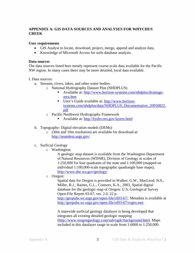
Appendix A 3 GIS Data & Analyses Whychus Ck
APPENDIX A: GIS DATA SOURCES AND ANALYSES FOR WHYCHUS CREEK User requirements
• GIS Analyst to locate, download, project, merge, append and analyze data. • Knowledge of Microsoft Access for soils database analysis.
Data sources The data sources listed here mostly represent coarse-scale data available for the Pacific NW region. In many cases there may be more detailed, local data available. I. Data sources:
a. Streams, rivers, lakes, and other water bodies: o National Hydrography Dataset Plus (NHDPLUS)
Available at: http://www.horizon-systems.com/nhdplus/drainage-area.htm
User’s Guide available at: http://www.horizon-systems.com/nhdplus/data/NHDPLUS_Documentation_20050822.pdf
o Pacific Northwest Hydrography Framework Available at: http://hydro.reo.gov/layers.html
b. Topography: Digital elevation models (DEMs)
o (30m and 10m resolution) are available for download at: http://seamless.usgs.gov/
c. Surficial Geology
o Washington: A geologic map dataset is available from the Washington Department of Natural Resources (WDNR), Division of Geology at scales of 1:250,000 for four quadrants of the state and 1:100,000 (mapped on individual 1:100,000-scale topographic quadrangle base maps); http://www.dnr.wa.gov/geology/
o Oregon: Spatial data for Oregon is provided in Walker, G.W., MacLeod, N.S., Miller, R.J., Raines, G.L., Connors, K.A., 2003, Spatial digital database for the geologic map of Oregon: U.S. Geological Survey Open-File Report 03-67, ver. 2.0, 22 p. http://geopubs.wr.usgs.gov/open-file/of03-67/. Metadata is available at http://geopubs.wr.usgs.gov/open-file/of03-67/orgeo.met. A statewide surficial geology datalayer is being developed that integrates all existing detailed geologic mapping (http://www.oregongeology.com/sub/ogdc/background.htm). Maps included in this datalayer range in scale from 1:6000 to 1:250,000.

Appendix A 4 GIS Data & Analyses Whychus Ck
Currently eastern Oregon is completed but new parts of the state are being released annually through 2009. These data were not used as they were not complete yet.
d. Hydric and organic soils • STATSGO Soils
o State Soil Geographic (STATSGO) database data are generally used for large (i.e. regional, multi-state, state, etc.) areas and are generalizations of more detailed SSURGO survey maps.
o STATSGO data and documents describing their use can be downloaded by state at: http://www.ncgc.nrcs.usda.gov/products/datasets/statsgo/
o You can join the spatial and tabular data by using either the "mukey" or "musym" since both are unique nationwide.
• SSURGO Soils
o The Soil Survey Geographic (SSURGO) database is the most detailed level of soil geographic data available. There are both spatial data (GIS files) as well as tabular data (Access databases) that go with the files. The 3D soils data are aggregated into polygons and each map unit symbol has one map unit name (1:1 relationship between musym and muname). Each map unit can have multiple soil components (1:many relationship between mapunits and components). Each component can have multiple horizons (1:many relationship between components and horizons).
o SSURGO data can be downloaded by county at: http://soildatamart.nrcs.usda.gov/.
o SSURGO metadata and User’s guides are available at: http://soildatamart.nrcs.usda.gov/SSURGOMetadata.aspx
o Download both the spatial and tabular data. You will then have to import the text files into the empty Access database (see readme file for instructions). Once the Access database is populated, you can join tables to the spatial data by the "mukey" field. It is a unique integer nationwide. The "musym" should not be used because it is not unique across soil survey area boundaries.
o Querying Soils Data:
Both the SSURGO and STATSGO data can be viewed and queried by an extension called the Soil Data Viewer. The soils data viewer is an extension that allows users to create soil-based thematic maps. It is very user-friendly and can provide excellent generalized information.
• ArcGIS Soils Data Viewer: http://soildataviewer.nrcs.usda.gov/
• ArcView Soils Data Viewer: http://www.itc.nrcs.usda.gov/soildataviewer/
Queries for hydric soils, hydric group and organic soils can be performed using the soil data viewer although the output is more general than specific.
Appendix A 5 GIS Data & Analyses Whychus Ck
For example, using the soil data viewer for hydric soils provides information on whether each map unit contains all, no, or partial hydric soils. A more specialized query could provide information such as percent hydric of the dominant soil component. More specialized queries can be complicated, but the NRCS provides excellent data specialists who are very helpful. If specialized queries are needed follow the link http://soils.usda.gov/contact/mlra_offices/ to an interactive map of the regional soil survey offices. If you click on a region it will pull up a directory for that office. The person to contact has a job title of "Soil Data Quality Specialist". Some of the office directories also identify the database manager. Someone in each office should be able to help users of the soil survey data with MS Access queries.
e. Precipitation o Precipitation isohyetals for the United States can be obtained from:
http://www.ocs.orst.edu/prism/ o We suggest using the average annual precipitation over a 30-year time
period. These data are available from 1961-1990 and from 1971-2000. Given climate change issues, it may be best to use the latter range.
f. Springs
o USGS Geographic Place Names data available at: http://www.gis.state.or.us/data/alphalist.html
o Flir GIS data o Pacific Northwest Hydrography Framework, available at:
http://hydro.reo.gov/layers.html o Hydrographic coverages (i.e., streams/rivers) often have springs identified.
g. Ecosystems and Species of Conservation Concern
o The Nature Conservancy ecoregional assessments o GIS data may be available through:
The Nature Conservancy field offices www.nature.org Natural Heritage Programs Streamnet data available at: http://www.streamnet.org/online-
data/GISData.html Data available from Subbasin Planning:
http://www.nwcouncil.org/fw/subbasinplanning/Default.htm National Land Cover Dataset is available at:
http://www.epa.gov/mrlc/nlcd.html Current habitats data is available at: http://www.nwhi.org/ National Wetlands Inventory (NWI)
• Available at: http://www.fws.gov/nwi/ • You will need to download and append or merge these data
at 1:24,000 scale if available. • Codes can be interpreted at:
http://wetlandsfws.er.usgs.gov/codes.html. Unfortunately there isn’t an automated way to do this.

Appendix A 6 GIS Data & Analyses Whychus Ck
II. Other data that may be useful a. Aquifers
o The Groundwater Atlas of the United States is available at: http://capp.water.usgs.gov/gwa/index.html
o The GIS data are available at: http://nationalatlas.gov/atlasftp.html?openChapters=chpgeol%2Cchpwater#chpwater
Appendices 7 Monitoring Wells
APPENDIX B: MONITORING WETLAND HYDROLOGY USING WELLS The hydrologic regime is the most important controlling factor of wetland species composition and ecosystem processes. Many species, particularly plants, respond primarily to the depth, duration and timing of flooding. Concentrations of dissolved oxygen, soil development, nutrient cycling, and carbon fluxes are among the processes influenced by spatial or temporal fluctuations in the depth of the water table. Monitoring wetland hydrology is often called for to establish baseline conditions and measure the response of a wetland to hydrologic alterations in the surrounding watershed. Activities that could affect wetland hydrology include upstream water withdrawals for a surface water-dominated wetland, and local groundwater pumping for a groundwater-dominated wetland. The first step in developing a monitoring program is to create a conceptual water budget for the wetland (Appendix C). To monitor wetland hydroperiod, two simple devices are used: staff gages and wells. Staff gages, also used in lakes and streams, are simple rulers installed in wetlands with above-ground water throughout the year. Their elevation is surveyed so that numbered gradations marked along the ruler can be converted to real surface water elevations. When monitored, the observer records the water level. The use of staff gages will not be discussed further in this document. For wetlands with a water table that drops below the soil surface, the hydroperiod can be monitored by installing wells in which the water level is measured. The water level in the wells should be monitored at least several times over the course of the growing season, depending on how much the water table fluctuates. The ground elevation and height of the wells also need to be surveyed so the water level in the well can be converted to a real elevation. For wetlands that experience freezing temperatures in the winter, the wells often need to be resurveyed every year to account for frost heave. The wells should be installed in transects perpendicular to the direction of water flow. In larger wetlands, several transects may be necessary. If resources are limited and only a small number of wells can be installed, they should be evenly spaced across the wetland. To develop a rigorous wetland hydrology monitoring program, it is always advisable to contact an expert who can help in the monitoring design. Correct installation of monitoring wells is essential for the data to be meaningful. It is relatively easy to install wells in peat (organic) soils. They can be fitted with a point and pushed down into the peat to the desired depth. It is more difficult to install monitoring wells in mineral soils. This requires augering a hole, installing the well, backfilling the hole, and capping it at the top. More detailed well installation instructions can be found online. Additional sources are listed at the end of this appendix. There are two types of monitoring wells: water table wells and piezometers. Making this distinction is important because the two well types are constructed differently and produce different kinds of data with different uses.
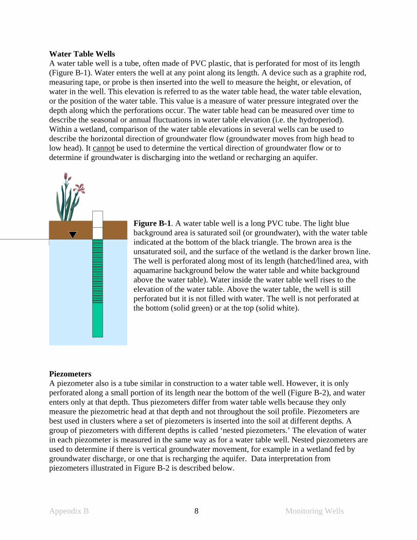
Appendix B 8 Monitoring Wells
Water Table Wells A water table well is a tube, often made of PVC plastic, that is perforated for most of its length (Figure B-1). Water enters the well at any point along its length. A device such as a graphite rod, measuring tape, or probe is then inserted into the well to measure the height, or elevation, of water in the well. This elevation is referred to as the water table head, the water table elevation, or the position of the water table. This value is a measure of water pressure integrated over the depth along which the perforations occur. The water table head can be measured over time to describe the seasonal or annual fluctuations in water table elevation (i.e. the hydroperiod). Within a wetland, comparison of the water table elevations in several wells can be used to describe the horizontal direction of groundwater flow (groundwater moves from high head to low head). It cannot be used to determine the vertical direction of groundwater flow or to determine if groundwater is discharging into the wetland or recharging an aquifer.
Figure B-1. A water table well is a long PVC tube. The light blue background area is saturated soil (or groundwater), with the water table indicated at the bottom of the black triangle. The brown area is the unsaturated soil, and the surface of the wetland is the darker brown line. The well is perforated along most of its length (hatched/lined area, with aquamarine background below the water table and white background above the water table). Water inside the water table well rises to the elevation of the water table. Above the water table, the well is still perforated but it is not filled with water. The well is not perforated at the bottom (solid green) or at the top (solid white).
Piezometers A piezometer also is a tube similar in construction to a water table well. However, it is only perforated along a small portion of its length near the bottom of the well (Figure B-2), and water enters only at that depth. Thus piezometers differ from water table wells because they only measure the piezometric head at that depth and not throughout the soil profile. Piezometers are best used in clusters where a set of piezometers is inserted into the soil at different depths. A group of piezometers with different depths is called ‘nested piezometers.’ The elevation of water in each piezometer is measured in the same way as for a water table well. Nested piezometers are used to determine if there is vertical groundwater movement, for example in a wetland fed by groundwater discharge, or one that is recharging the aquifer. Data interpretation from piezometers illustrated in Figure B-2 is described below.
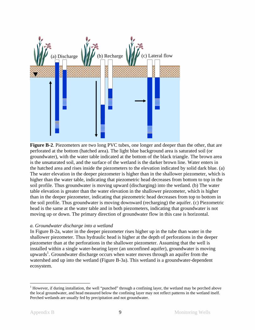
Appendix B 9 Monitoring Wells
(c) Lateral flow(a) Discharge (b) Recharge
Figure B-2. Piezometers are two long PVC tubes, one longer and deeper than the other, that are perforated at the bottom (hatched area). The light blue background area is saturated soil (or groundwater), with the water table indicated at the bottom of the black triangle. The brown area is the unsaturated soil, and the surface of the wetland is the darker brown line. Water enters in the hatched area and rises inside the piezometers to the elevation indicated by solid dark blue. (a) The water elevation in the deeper piezometer is higher than in the shallower piezometer, which is higher than the water table, indicating that piezometric head decreases from bottom to top in the soil profile. Thus groundwater is moving upward (discharging) into the wetland. (b) The water table elevation is greater than the water elevation in the shallower piezometer, which is higher than in the deeper piezometer, indicating that piezometric head decreases from top to bottom in the soil profile. Thus groundwater is moving downward (recharging) the aquifer. (c) Piezometric head is the same at the water table and in both piezometers, indicating that groundwater is not moving up or down. The primary direction of groundwater flow in this case is horizontal. a. Groundwater discharge into a wetland In Figure B-2a, water in the deeper piezometer rises higher up in the tube than water in the shallower piezometer. Thus hydraulic head is higher at the depth of perforations in the deeper piezometer than at the perforations in the shallower piezometer. Assuming that the well is installed within a single water-bearing layer (an unconfined aquifer), groundwater is moving upwards1. Groundwater discharge occurs when water moves through an aquifer from the watershed and up into the wetland (Figure B-3a). This wetland is a groundwater-dependent ecosystem.
1 However, if during installation, the well “punched” through a confining layer, the wetland may be perched above the local groundwater, and head measured below the confining layer may not reflect patterns in the wetland itself. Perched wetlands are usually fed by precipitation and not groundwater.
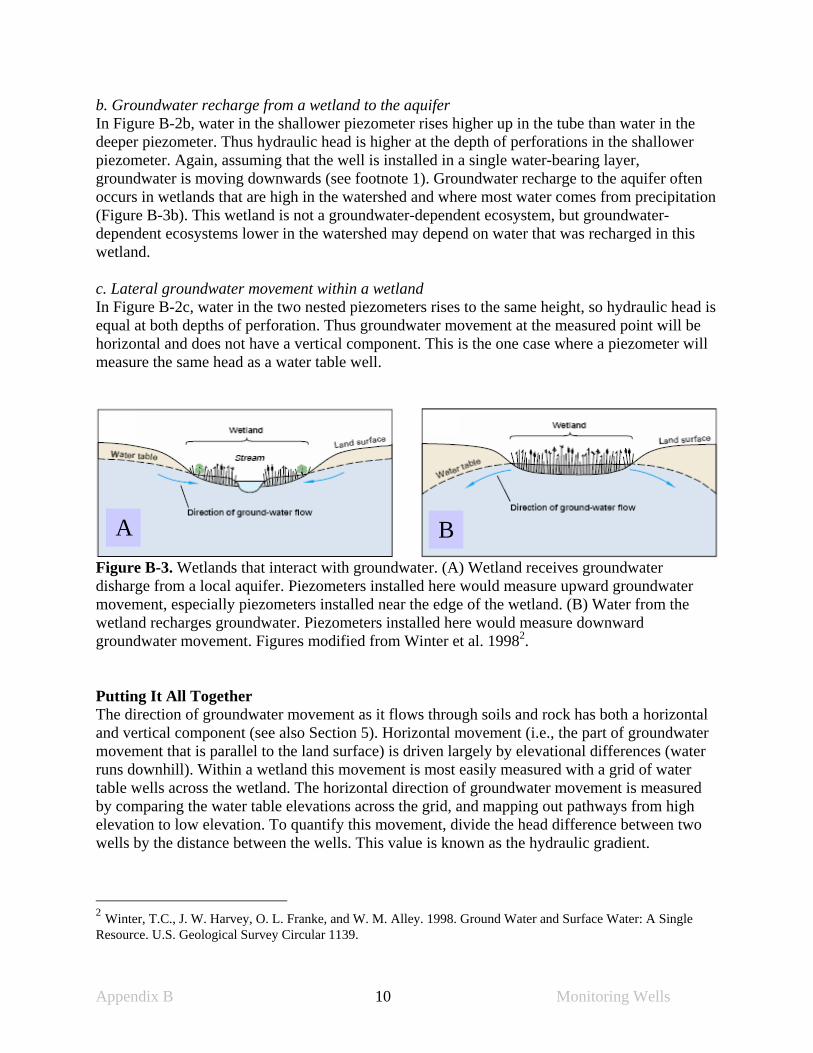
Appendix B 10 Monitoring Wells
b. Groundwater recharge from a wetland to the aquifer In Figure B-2b, water in the shallower piezometer rises higher up in the tube than water in the deeper piezometer. Thus hydraulic head is higher at the depth of perforations in the shallower piezometer. Again, assuming that the well is installed in a single water-bearing layer, groundwater is moving downwards (see footnote 1). Groundwater recharge to the aquifer often occurs in wetlands that are high in the watershed and where most water comes from precipitation (Figure B-3b). This wetland is not a groundwater-dependent ecosystem, but groundwater-dependent ecosystems lower in the watershed may depend on water that was recharged in this wetland. c. Lateral groundwater movement within a wetland In Figure B-2c, water in the two nested piezometers rises to the same height, so hydraulic head is equal at both depths of perforation. Thus groundwater movement at the measured point will be horizontal and does not have a vertical component. This is the one case where a piezometer will measure the same head as a water table well.
Figure B-3. Wetlands that interact with groundwater. (A) Wetland receives groundwater disharge from a local aquifer. Piezometers installed here would measure upward groundwater movement, especially piezometers installed near the edge of the wetland. (B) Water from the wetland recharges groundwater. Piezometers installed here would measure downward groundwater movement. Figures modified from Winter et al. 19982. Putting It All Together The direction of groundwater movement as it flows through soils and rock has both a horizontal and vertical component (see also Section 5). Horizontal movement (i.e., the part of groundwater movement that is parallel to the land surface) is driven largely by elevational differences (water runs downhill). Within a wetland this movement is most easily measured with a grid of water table wells across the wetland. The horizontal direction of groundwater movement is measured by comparing the water table elevations across the grid, and mapping out pathways from high elevation to low elevation. To quantify this movement, divide the head difference between two wells by the distance between the wells. This value is known as the hydraulic gradient.
2 Winter, T.C., J. W. Harvey, O. L. Franke, and W. M. Alley. 1998. Ground Water and Surface Water: A Single Resource. U.S. Geological Survey Circular 1139.
A B
Appendix B 11 Monitoring Wells
Vertical groundwater movement that is not parallel to the land surface is driven largely by pressure gradients established by a combination of geologic and topographic forces. Vertical movement within the soil/rock profile usually is measured using piezometers. To quantify the vertical hydraulic gradient, divide the head difference between two piezometers within a nested set by the vertical distance between the perforated sections. The horizontal and vertical hydraulic gradients can then be compared to get a sense of the relative importance of vertical vs. horizontal groundwater movement. In general, wetlands that are dominated by horizontal water movement tend to have a large surface water contribution to the water budget. Wetlands that are found in rolling landscapes with more topography and those receiving obvious groundwater discharge will have more vertical groundwater movement. Additional sources of information Aller, L., T.W. Bennett, G. Hackett, R.J. Petty, J.H. Lehr, H. Sedoris, and D.M. Nielsen. 1990.
Handbook of Suggested Practices for the Design and Installation of Ground-water Monitoring Wells. National Water Well Association. Dublin, OH.
American Society for Testing and Materials. 1990. Standard Practice for design and Installation
of Groundwater Monitoring Wells in Aquifers. Designation D-5092, Philadelphia, PA. Driscoll, F. 1986. Groundwater and Wells. Johnson Division, St. Paul, MN. The Nature Conservancy. 1995. Hydrologic Monitoring Manual. TNC, Arlington, VA. WRP Technical Note HY-IA-3.1. Installing Monitoring Wells/Piezometers in Wetlands.
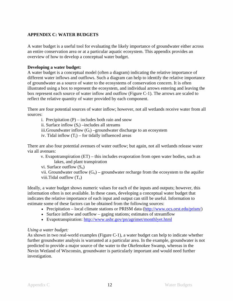
Appendix C 12 Water Budgets
APPENDIX C: WATER BUDGETS A water budget is a useful tool for evaluating the likely importance of groundwater either across an entire conservation area or at a particular aquatic ecosystem. This appendix provides an overview of how to develop a conceptual water budget. Developing a water budget: A water budget is a conceptual model (often a diagram) indicating the relative importance of different water inflows and outflows. Such a diagram can help to identify the relative importance of groundwater as a source of water to the ecosystems of conservation concern. It is often illustrated using a box to represent the ecosystem, and individual arrows entering and leaving the box represent each source of water inflow and outflow (Figure C-1). The arrows are scaled to reflect the relative quantity of water provided by each component. There are four potential sources of water inflow; however, not all wetlands receive water from all sources: i. Precipitation (P) – includes both rain and snow ii. Surface inflow (Si) –includes all streams iii.Groundwater inflow (Gi) –groundwater discharge to an ecosystem iv. Tidal inflow (Ti) – for tidally influenced areas There are also four potential avenues of water outflow; but again, not all wetlands release water via all avenues:
v. Evapotranspiration (ET) – this includes evaporation from open water bodies, such as lakes, and plant transpiration
vi. Surface outflow (So) vii. Groundwater outflow (Go) – groundwater recharge from the ecosystem to the aquifer viii.Tidal outflow (To) Ideally, a water budget shows numeric values for each of the inputs and outputs; however, this information often is not available. In these cases, developing a conceptual water budget that indicates the relative importance of each input and output can still be useful. Information to estimate some of these factors can be obtained from the following sources:
• Precipitation – local climate stations or PRISM data (http://www.ocs.orst.edu/prism/) • Surface inflow and outflow – gaging stations; estimates of streamflow • Evapotranspiration: http://www.usbr.gov/pn/agrimet/monthlyet.html
Using a water budget: As shown in two real-world examples (Figure C-1), a water budget can help to indicate whether further groundwater analysis is warranted at a particular area. In the example, groundwater is not predicted to provide a major source of the water to the Okefenokee Swamp, whereas in the Nevin Wetland of Wisconsin, groundwater is particularly important and would need further investigation.
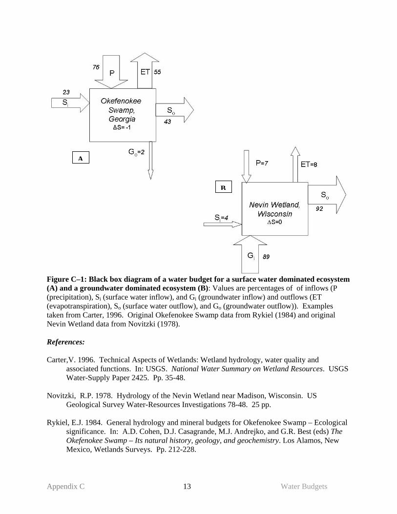
Appendix C 13 Water Budgets
Figure C–1: Black box diagram of a water budget for a surface water dominated ecosystem (A) and a groundwater dominated ecosystem (B): Values are percentages of of inflows (P (precipitation), Si (surface water inflow), and Gi (groundwater inflow) and outflows (ET (evapotranspiration), So (surface water outflow), and Go (groundwater outflow)). Examples taken from Carter, 1996. Original Okefenokee Swamp data from Rykiel (1984) and original Nevin Wetland data from Novitzki (1978). References: Carter,V. 1996. Technical Aspects of Wetlands: Wetland hydrology, water quality and
associated functions. In: USGS. National Water Summary on Wetland Resources. USGS Water-Supply Paper 2425. Pp. 35-48.
Novitzki, R.P. 1978. Hydrology of the Nevin Wetland near Madison, Wisconsin. US
Geological Survey Water-Resources Investigations 78-48. 25 pp. Rykiel, E.J. 1984. General hydrology and mineral budgets for Okefenokee Swamp – Ecological
significance. In: A.D. Cohen, D.J. Casagrande, M.J. Andrejko, and G.R. Best (eds) The Okefenokee Swamp – Its natural history, geology, and geochemistry. Los Alamos, New Mexico, Wetlands Surveys. Pp. 212-228.
A
B
Appendix D Tools 14 Introduction
APPENDIX D: TOOLS FOR UNDERSTANDING GROUNDWATER AND BIODIVERSITY
1. Modeling recharge areas:.......................................................................................... 15 2. Seepage runs: ............................................................................................................ 17 3. Baseflow – percentage of annual streamflow ........................................................... 18 4. Water table data ........................................................................................................ 19 5. Forward Looking Infrared Remote Sensing (FLIR): ................................................ 20 6. Water Chemistry Analysis: ....................................................................................... 21 7. Environmental Tracer Analysis: ............................................................................... 24 References:.................................................................................................................... 27
Introduction: In some cases, more detailed information than can be obtained through use of the methods guide will be needed about groundwater and its relationship to biodiversity. This appendix describes some additional tools that can be used to understand different aspects of groundwater processes and the relevance of groundwater to particular components of biodiversity. It is not meant to be an exhaustive discussion of these tools; as such, it provides an overview of just some of the tools that are available. Each section describes some of the reasons that the tool might be used, how the tool works, where it has been applied, its data requirements, and some of its limitations. Actual application of any of these tools will require consultation with experts to ensure the tool selected is an appropriate and efficient choice. Another source of information regarding tools for identifying GDEs and understanding the importance of groundwater to different ecosystems can be found in Clifton et al. (2007). This document, produced in Australia, is online at http://www.lwa.gov.au/environmentalwater/library/scripts/objectifyMedia.aspx?file=pdf/98/57.pdf&siteID=8&str_title=REM1%20Report1_Assessment%20Tool%20Box_Final.pdf. Tables 2.1 and 2.2 in this document highlight a suite of tools and indicate which ones are most useful for specific situations. Details about each of the tools are provided in the document text.
Appendix D Tools 15 Modeling recharge areas
1. Modeling recharge areas: Why you might consider using this approach: • If you need to know more precisely which areas on the landscape provide recharge • If you need to know how much recharge is provided by specific areas Model Name: Deep Percolation Model What it does: This model produces a map of recharge rates across the study area; the area is divided into cells and recharge rates are calculated for each cell. For each cell of the grid, a daily water balance is calculated; from this, monthly and annual mean recharge rates for each cell can be calculated. Where it has been used: The Deep Percolation Model was developed by Bauer and Vaccaro of the USGS (1987) for a regional analysis of the Columbia Plateau aquifer in eastern Washington. In addition, this has been applied in the Upper Deschutes Basin (Gannett, et al., 2001), to the Goose Lake Basin of Oregon and California (Morgan, 1988), and to the Portland Basin of Oregon and Washington (Snyder et al., 1994).
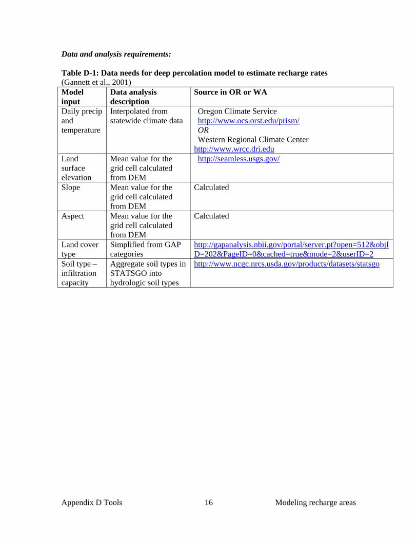
Appendix D Tools 16 Modeling recharge areas
Data and analysis requirements: Table D-1: Data needs for deep percolation model to estimate recharge rates (Gannett et al., 2001) Model input
Data analysis description
Source in OR or WA
Daily precip and temperature
Interpolated from statewide climate data
Oregon Climate Service http://www.ocs.orst.edu/prism/ OR Western Regional Climate Center
http://www.wrcc.dri.edu Land surface elevation
Mean value for the grid cell calculated from DEM
http://seamless.usgs.gov/
Slope Mean value for the grid cell calculated from DEM
Calculated
Aspect Mean value for the grid cell calculated from DEM
Calculated
Land cover type
Simplified from GAP categories
http://gapanalysis.nbii.gov/portal/server.pt?open=512&objID=202&PageID=0&cached=true&mode=2&userID=2
Soil type – infiltration capacity
Aggregate soil types in STATSGO into hydrologic soil types
http://www.ncgc.nrcs.usda.gov/products/datasets/statsgo
Appendix D Tools 17 Seepage runs
2. Seepage runs: Why you might consider using this approach: • You need to know the general locations of groundwater inputs (or losses) to a river • You need to quantify groundwater inputs from a spring or other known groundwater
discharge into a river • You want to know which river reaches are gaining and which are losing at a certain
point in time What it does: Depending on the elevation of the water table relative to the stream elevation, groundwater can either move into streams or move out of streams. Stream reaches into which groundwater is entering are called ‘gaining reaches’; those from which groundwater is leaving are called ‘losing reaches’. Seepage runs quantify the amount of gain or loss that occurs in specific reaches. Where it has been used: This technique is very common and has been used in numerous locations. In Oregon, some of the areas it has been used are Upper Deschutes River (Gannett et al., 2001), Lost River (Grondin, 2004), and Willamette River Basin (Lee and Risley, 2002) by the Oregon Water Resources Division and the U.S. Geological Survey. In Washington, this analysis has been completed at many sites including Seibert Creek (Clallam County, Larson, 2004), Walla Walla River (Marti, 2005), and Wenatchee River (Kiimsey, 2005). See http://www.ecy.wa.gov/biblio/groundwater.html and http://www.ecy.wa.gov/programs/eap/wsb/wsb_Geology-and-Groundwater.html for a more complete list of where groundwater studies, including seepage runs, have been completed. Data and analysis requirements: Seepage runs require discharge data at multiple locations at a single point in time (or within a very short time period). Both the mainstem and the tributaries must be measured, as well as diversions, to evaluate the changes in discharge along the stream system. Limitations: The gains or losses must be greater than the uncertainty associated with the flow measurement method. Uncertainty of measurements is usually expressed as a percentage of total flow; as a result, it is possible to detect smaller losses or gains into streams with lower discharge than in streams with higher discharge (Lee and Risley, 2002).
Appendix D Tools 18 Baseflow analysis
3. Baseflow – percentage of annual streamflow Why you might consider using this approach: • You want to confirm that groundwater is a significant portion of streamflow in your
watershed • You want to compare the relative importance of groundwater inputs between two
watersheds What it does: This technique is based upon the methods of hydrograph separation which, until recently, required a manual separation of streamflow into baseflow (groundwater discharge) and runoff. Now, several programs that automate this process are in the public domain. All produce an estimate of the percentage of annual or monthly streamflow that is supplied by baseflow. Where it has been used: • Using the HYSEP program (Sloto and Crouse, 1996), this method has been
applied to 294 streams in Washington (Sinclair and Pitz, 1999; see Methods Guide, section 3). The program produces tables of the proportion of annual streamflow that is provided by baseflow on a monthly or annual basis.
• Using the PART program (Rutledge, 1998), this method has been applied to
streams in the Willamette Basin (Lee and Risley, 2002). Data and analysis requirements: Daily mean stream discharge data from a gaging station are required; if it is available, these can be downloaded from the National Water Information System maintained by USGS. Limitations:
• A reasonable length of record of daily gage data is required; Sinclair and Pitz (1999) required that three years of record be available.
• Calculations cannot occur in streams with snowmelt as the volume of this water is included in the baseflow estimates, producing an overestimate of baseflow. Analysts have accounted for this issue by only examining months when snowmelt was not a contributor to streamflow.
• Measurements are limited if streams cannot be regulated due to dams, diversions, water treatment plants, releases from mines/quarries, etc.
• Many authors recommend applying this method to basins that are greater than four to 500 square miles; however, it has been applied to much smaller basins.
• This method provides an estimate of baseflow for the entire basin above the gage, not an individual reach.
• HYSEP is available for use in a DOS environment but not Windows.
Appendix D Tools 19 Water table data
4. Water table data Why you might consider using this approach:
• You need information on the flow direction of groundwater or on the water table elevation or geometry
What it does: Using water table data from wells and elevations of springs, a contour map of water table elevations (similar to a topo map for land surface) can be constructed. Water then is assumed to move perpendicular to the contour lines – from areas of high elevation (or high head) to areas of low elevation (low head). Where it has been used: Upper Deschutes River Basin (Gannett et al., 2001) Data and analysis requirements: The data required are water table elevations at well sites and elevations of springs or other points of groundwater discharge. • Water levels for monitored wells in Oregon are available from OWRD at
http://www.wrd.state.or.us/OWRD/GW/well_data.shtml#View_Water_Level_Data and from USGS at http://waterdata.usgs.gov/or/nwis/gw.
• In Washington, websites containing water tables of wells are available through the
Washington State Department of Ecology and the USGS at the following websites: http://apps.ecy.wa.gov/welllog http://www.ecy.wa.gov/eim/ http://wa.water.usgs.gov/data/gw/ http://www.ecy.wa.gov/services/gis/ for Arcview data.
These data can then be mapped using either a GIS program or software that draws contour lines based on the water depth data (e.g. SURFER). Limitations:
• Applies to unconfined aquifers only • Maps are usually highly interpretive, particularly at large scales • Data are almost always sparse and poorly distributed spatially.

Appendix D Tools 20 Stable Isotope Analysis
5. Forward Looking Infrared Remote Sensing (FLIR): Why you might consider using this approach:
• Groundwater discharge is hard to identify and you need its location • Water temperature is a threat to your target
What it does: FLIR is an airborne remote sensing tool that records temperatures on the earth’s surface. It can be used to map temperature patterns in streams and lakes, such as cool water from groundwater discharge. Where it has been used: FLIR data are available for many locations in Oregon. Examples of its use include the Whychus Creek drainage in the Deschutes River Basin, the Lower Crooked River in the Deschutes River Basin (Watershed Sciences, LLC, 2000 and 2004), Bridge Creek and Little Blitzen River in the Malheur Basin, Wood River and Lost River in the Upper Klamath Basin, and parts of the Umatilla Basin and Grand Ronde Basin. Many of these data were collected as part of establishing TMDLs for temperature (http://www.oregondeq.com/wq/tmdls/tmdls.htm). Additionally in Washington state, FLIR has been used on the Nooksack River (Cox et al., 2005) and Sammamish River (Carey, 2001). Data and analysis requirements: Data collection requires flying the area with an aircraft that has a sensor attached on a gyroscopic mounted to its underside. Flying with a video camera allows for intersection of the image with the thermal data. Each pixel of thermal data is analyzed and an Arc View coverage of data points is produced. In addition to the flight, field measurements of stream temperature should also be made in order to ground truth the remote sensing results. Limitations: Cost is the biggest limitation.
Appendix D Tools 21 Water chemistry
6. Water Chemistry Analysis: Why you might consider using this approach:
• To identify whether groundwater is a major source of water to a river, lake, or wetland ecosystem
What it does: Waters in aquatic ecosystems are usually a combination of water from different sources (precipitation, surface water, or groundwater). If the pH or electrical conductivity is known for the different sources, the water chemistry of the ecosystem can be used to deduce the relative contribution of the possible sources. This concept is referred to as a simple mixing model. Where it has been used: The Washington State Department of Health uses pH, temperature and conductivity to identify whether groundwater is influenced by surface water (http://www.doh.wa.gov/ehp/dw/Publications/331-230_Potential_GWI_Sources_WQM.pdf ) Data and analysis requirements:
Electrical Conductivity (EC): (also known as specific conductance or electrical conductance)
What is EC?: EC is a measure of the capacity of water to conduct an electrical current; it is the reciprocal of resistivity and has units of µS/cm (S= siemens). As dissolved ions increase the amount of electrical current that can be conducted, a higher conductivity value indicates a greater amount of total dissolved salts or ions.
How to measure EC: A conductivity meter, with temperature correction, can be used to measure EC. Specific EC (the conductivity at 25°C) is the usual reporting parameter; this ensures that the effect of temperature on conductivity has been removed and allows for comparison between water samples of different temperatures.
Interpreting EC data: Many factors affect conductivity. EC will increase as: i. The proportion of water provided by precipitation decreases:
Precipitation usually has a low EC. In Washington, values are often less than 15 µS/cm but range to 80 µS/cm.
ii. The size of the watershed increases: Larger watersheds usually generate more surface runoff, providing not only more water to wetlands, lakes and streams but also providing more opportunity for salts or ions to be removed from the soils by the water.
iii. The solubility of the geologic substrate increases: As groundwater moves through different geologic substrates, water has time to dissolve some of the material and increase the dissolved salt concentrations. More soluble substrates, likely to increase conductivity of groundwater, are limestone and sandstone, whereas less soluble substrates are bedrock such as granite.
Appendix D Tools 22 Water chemistry
iv. Proximity to the ocean increases: Salts from ocean water, both in terms of salt water intrusion into groundwater and contamination by salt spray, can increase conductivity values.
v. Other sources of ions are added to water: Wastewater additions, urban or agricultural runoff, and atmospheric inputs of ions can increase EC.
vi. Evaporation increases: in hot, dry areas, evaporation of water from lakes or wetlands can increase the concentration of salts, increasing conductivity.
vii. Bacterial activity and decomposition increase. In general, groundwater will have higher EC than precipitation (Hem, 1985) or non-floodplain surface waters (Aldous, unpublished data); however it is important to evaluate the other six factors discussed above in order to ensure high EC is not occurring for some other reason before concluding that groundwater is important to a wetland or stream.
pH:
What is pH?: pH is a measure of the concentration of hydrogen ions in water. It is the negative log of the concentration of hydrogen ions. The higher the pH, the fewer the hydrogen ions. Because pH is measured on a log scale, a pH increase of 1.0 is a 10-fold decrease in the number of hydrogen ions. It is measured on a scale of 0 to 14. A pH of 7 is neutral, greater than 7 is basic, and less than 7 is acidic.
How to measure pH: pH can be measured using relatively inexpensive pH meters.
Interpreting pH data: Most wetlands are at least slightly acidic. Wetland pH is a function of ecological processes that occur within the wetland and the pH of contributing waters. Within a wetland, acidity can be generated from organic acids produced from incomplete decomposition that occurs under permanently saturated, anoxic conditions. Sphagnum mosses found in poor fens also can generate acidity from cellular ionic exchange. When aquatic plants, algae, and cyanobacteria photosynthesize, they use dissolved carbonic acid rather than CO2 gas, and in the process they consume hydrogen ions, thus raising pH. This is most apparent in highly eutrophic waters where there is a lot of algal and plant biomass.
Contributing waters can alter wetland pH in several ways. If the water source contains dissolved cations or is alkaline, this can buffer the pH and prevent it from dropping due to organic acid production or Sphagnum acid release. On the other hand, wetlands dominated by precipitation will have slightly acidic pH and no buffering capacity; as a result, they are more sensitive to acidic inputs such as acid precipitation. Similarly, wetlands dominated by groundwater that travels over highly insoluble bedrock, such as granite, will have little buffering capacity and the pH may be quite low.
Appendix D Tools 23 Water chemistry
Wetlands with low base cation concentrations, such as bogs dominated by precipitation inputs and poor fens which receive groundwater that has flowed through bedrock of low solubility, have pH values from three to five. Wetlands that are dominated by surface water or groundwater from bedrock with intermediate solubility have pH values in the range of six to seven. Wetlands that receive groundwater from bedrock with high solubility have pH values that range from seven to eight. If a wetland has very high pH, for example eight to ten, it can be an indication that plant and algal biomass is very high due to nutrient loading.
Where to find water quality data for groundwater, precipitation, and surface water:
Precipitation: EPA’s CASTNET dataset summarizes information from National Atmospheric Deposition Program study sites; these include wet deposition sites which are precipitation sites (http://www.epa.gov/castnet/site.html). Water on the Web indicates the precipitation pH is between 5 and 6.
Groundwater: Water chemistry data are available for wells studied by the
USGS through the National Water Information Service. For Oregon this is found at http://waterdata.usgs.gov/or/nwis/qw and for Washington at http://waterdata.usgs.gov/wa/nwis/current/?type=qwsearch. Additional information for Oregon is managed by the Department of Environmental Quality and available through the LASAR database - http://deq12.deq.state.or.us/lasar2/. In Washington, a list of places where groundwater quality has been studied and data may be available is found at the Department of Ecology’s website at (http://www.ecy.wa.gov/biblio/watershed.html.
Surface water: Water chemistry data are also available for surface waters
through the USGS National Water Information Service (same as above) and through the EPA’s STORET database (http://www.epa.gov/storet/dbtop.html
Limitations: Given the number of factors unrelated to groundwater that can cause variability in water chemistry, such as in-site water cycling and use by plants and microbes, it is best to have any analysis reviewed by someone familiar with water chemistry, and to use these data in conjunction with other evidence.
Appendix D Tools 24 Environmental Tracer Analysis
7. Environmental Tracer Analysis: Environmental tracer analysis uses parameters present in water to indicate the likely source of that water. This can be useful for indicating whether groundwater is an important source of water to an ecosystem. The ideal tracer is inert (i.e., non reactive), is easily measured, has low background concentrations, and has different abundances in other (non-groundwater) water sources. Three common environmental tracers are (Cook et al., 2007):
i) chloride (Cl-) ii) stable isotopes of hydrogen (2H) and oxygen (18O) iii) radon (222Rn).
Each of these tracers can be used to infer the importance of groundwater to an ecosystem, but each method involves slight differences in interpretation (Cook et al., 2007). With increasing groundwater inputs, Cl- concentrations increase, 2H and 18O decrease and 222Rn increases. Cl- is a conservative tracer, meaning that it remains in a body of water for time periods on the order of years. 2H and 18O are lost through evaporation and as a result can indicate the presence of groundwater inputs over a period of months. 222Rn has a half life of 3.8 days and as a result indicates groundwater inputs over the previous few days. The stable isotopes 2H and 18O and the element 222Rn are most useful for indicating recent inflows of groundwater, and so they are discussed in more detail below. Why you might consider using this approach: • To determine whether and how much shallow groundwater is entering an ecosystem
What it does: A. Stable isotopes 2H and 18O: The elements of water – hydrogen and oxygen – are available as multiple stable isotopes. All isotopes of an element contain the same number of protons but different numbers of neutrons. More neutrons yield heavier isotopes. Hydrogen has two stable isotopes with the following abundances: 1H (99.9844%), and 2H (0.0156%)3. Oxygen has three stable isotopes with the following abundances: 16O (99.763%), 17O (0.0375%), and 18O (0.1995%). Through a process known as fractionation, the isotopes in water undergo physical and chemical reactions and transformations after water falls as precipitation on the earth’s surface. In surface water, the processes of evaporation and transpiration favor the lighter isotopes over the heavier ones. For example, during evaporation, the heavier molecules (2H2
18O) become more highly concentrated in the water as the lighter molecules (1H216O)
vaporize. Once water enters the groundwater, the isotopic composition of oxygen and hydrogen remain relatively stable in the proportions given above until the water emerges
3 2H is commonly referred to as deuterium, or 2D
Appendix D Tools 25 Environmental Tracer Analysis
at the point of discharge (Caldwell, 1998)4; as a result, groundwater has fairly low concentrations of the heavier isotopes. These differences in isotopic signature can be used to tease apart groundwater source areas to an ecosystem as well as the water sources used by different plants. By taking groundwater isotope samples across a watershed, scientists can determine the relative contributions of local and regional groundwater, surface water, and precipitation. Another application takes advantage of the fact that plant roots can have access to different water sources, depending on rooting depth and water availability. The water found in plant xylem (the primary conduit for water in vascular plants) will have one signature if the plant roots are taking up groundwater, and another signature if they are taking up surface water. By sampling the xylem isotopic composition, as well as the possible sources (groundwater, soil water), it is possible to infer the water source being used by the plants. B. Radon Radon (222Rn ) is a naturally occurring radioactive element and a decay product of radium-226. It occurs in all soils and rocks to varying degrees (Cook et al., 2007). As groundwater flows through soils and geologic deposits, it absorbs 222Rn. Surface waters do not gain as much radon as groundwater, and deeper groundwater tends to have different concentrations of 222Rn than shallower groundwater (Le Druillennec et al., 2005). As a result, higher 222Rn levels can be used to indicate groundwater discharge into an ecosystem and to estimate its importance. Where it has been used: Stable isotopes: • In pinyon-juniper ecosystems of Utah and Arizona, USA, the dominant trees use a
combination of soil water and precipitation, but not groundwater (Williams and Ehleringer, 2000).
• In the species-rich tropical forests of Barro Colorado Island, Panama, there is a partitioning of water sources among several canopy tree species during the dry season. These trees were shown to use increasingly deeper sources of water over the course of the dry season (Meinzer et al. 1999).
• In Inner Mongolia, China, water use by an introduced tree species was compared to two native species. The introduced species was shown to use deeper groundwater and to have lower water use efficiency, thus contributing to water depletion in this region. (Ohte et al. 2003)
• In the Upper Deschutes Basin, Oregon, USA, stable isotope concentrations were used to tightly link canal-water to nearby groundwater, indicating leaking canals supplied some groundwater recharge (Caldwell, 1998)
Radon:
• In Australia, groundwater inputs to lakes and wetlands were estimated using radon (Cook et al., 2007; White and Wood, 2007).
4 This is true at low temperatures; at high temperatures, the concentration of 18O can increase.
Appendix D Tools 26 Environmental Tracer Analysis
• In the Gulf of Mexico, groundwater discharge into the ocean was identified using radon and methane (Cable et al., 1996)
Data and analysis requirements: • Water samples must be collected from all possible sources. If plant water use is of
interest, samples will also need to come from the plant xylem. • Water sources may include: shallow and/or deep groundwater, shallow and/or deep
soil water, surface water, fog, and precipitation. • Analysis is done in a lab with a natural abundance isotope mass spectrometer or in the
field using an ionization chamber. Limitations: Cost and access to the isotopic analysis equipment are the biggest limitations.
Appendix D Tools 27 References
References: Bauer, H.H. and Vaccaro, J.J. 1987. Documentation of a deep percolation model for
estimating ground-water recharge: US Geological Survey Open-File-Report 86-536, 180 pp.
Cable, J.E., G.C. Bugna, W.C. Burnett, & J.P. Chanton.1996. Application of 222Rn and
CH4 for assessment of groundwater discharge to the coastal ocean. Limnology & Oceanography. 41(6):1347-1353.
Caldwell, R. R. 1998. Chemical study of regional ground-water flow and ground-
water/surface-water interaction in the Upper Deschutes Basin, Oregon. USGS Water-Resources Investigations Report 97-4233. 49 pp.
Carey, B. 2001. Groundwater/Surface Water Interactions In the Sammamish River: a
Preliminary Analysis. Quality Assurance Project Plan. Washington State Department of Ecology Environmental Assessment Program Report. 18 electronic pages. Available at: http://www.ecy.wa.gov/pubs/0103068.pdf
Clifton, C., B. Cossens, and C. McAuley. 2007. Project REM1- A framework for
assessing the environmental water requirements of groundwater dependent ecosystems: Report 1 Assessment Toolbox. Kent Town:Resource and Environmental Management Pty. Ltd. Document number: DB01-R002. 70 electronic pages. Available at: http://www.lwa.gov.au/environmentalwater/library/scripts/objectifyMedia.aspx?file=pdf/98/57.pdf&siteID=8&str_title=REM1%20Report1_Assessment%20Tool%20Box_Final.pdf
Cook, P.G., C. Wood, T. White, and C.T. Simmons. 2007. Estimating groundwater
discharge to lake and wetland ecosystems using environmental tracers. Presentation at the International Hydrogeology Association Groundwater and Ecosystems Conference, Lisbon, Portugal, September 17-21,2007.
Cox, S.E., F. W. Simonds, L. Doremus, R. L. Huffman, and R. M. Defawe. 2005.
Ground Water/Surface Water Interactions and Quality of Discharging Ground Water in Streams of the Lower Nooksack River Basin, Whatcom County, Washington. USGS Scientific Investigations Report 2005-5255. Available at: http://pubs.usgs.gov/sir/2005/5255/index.html
Dawson, T. E., R. C. Pausch, and H. M. Paker. 1998. The role of hydrogen and oxygen
stable isotopes in understanding water movement along the soil–plant–atmospheric continuum. Pages 169–183 in H. Griffiths, editor. Stable isotopes. BIOS Scientific Publishers, Oxford, UK.
Appendix D Tools 28 References
Ehleringer, J. R., and T. E. Dawson. 1992. Water uptake by plants: perspectives from stable isotope composition. Plant, Cell, and Environment 15: 1073-1082.
Ehleringer, J.R. and C.B. Osmond. 1989. Stable Isotopes. Pp. 281-300 in R.W. Pearcy, J. Ehleringer, H.A. Mooney, and P.W. Rundel, eds. Plant Physiological Ecology: Field Methods and Instrumentation. Chapman and Hall, New York, NY, U.S.A.
Gannett, M.W., K.E. Lite, Jr., D. S. Morgan, and C.A. Collins. 2001. Ground-Water
Hydrology of the Upper Deschutes Basin, Oregon. USGS Water-Resources-Investigations Report 00-4162. 78 pp. Available at: http://pubs.er.usgs.gov/usgspubs/wri/wri004162
Grondin, G.H. 2004. Groundwater in the eastern Lost River sub-basin, Langell, Yonna,
Swan Lake and Poe Valleys of southeastern Klamath County, Oregon. OWRD Groundwater Report No. 41. 171 pp. http://www.wrd.state.or.us/OWRD/GW/gw_report41.shtml
Hem, J.D. 1985. Study and interpretation of the chemical characteristics of natural water.
USGS Water-Supply Paper 2254. 272 electronic pages. Available at: http://pubs.er.usgs.gov/usgspubs/wsp/wsp2254
Kimsey, M. 2005. Groundwater data summary for the Wenatchee River watershed total
maximum daily limit study. Washington State Department of Ecology Publication No. 05-03-018. http://www.ecy.wa.gov/pubs/0503018.pdf
Larson, A. 2004. Groundwater contributions to Seibert Creek (Clallam County) during
the summer of 2003. WA State Department of Ecology Report No. 04-03-021. http://www.ecy.wa.gov/pubs/0403021.pdf
Le Druillennec, T.,. Tarits, G. Ielsch, L. Aquilina, G. Tymen, V. Ayraud, and O. Bour.
2005. Radon-222 measurements in groundwaters and rocks from fractured aquifer (Ploemeur, Britanny). Geophysical Research Abstracts, Vol. 7, 06584-2005. Available at: http://www.cosis.net/abstracts/EGU05/06584/EGU05-J-06584.pdf
Lee, K.K., and Risley, J.C., 2002, Estimates of Ground-Water Recharge, Base Flow, and
Stream Reach Gains and Losses in the Willamette River Basin, Oregon: U.S. Geological Survey Water-Resources Investigations Report 01-4215, 52 p., 1 plate. Available at: http://or.water.usgs.gov/projs_dir/willgw/reports.html
Marti, P.B. 2005. Assessment of surface water and groundwater interchange in the Walla
Walla Watershed. Washington State Department of Ecology. Publication No. 05-03-020. 67 pp. http://www.ecy.wa.gov/pubs/0503020.pdf
Appendix D Tools 29 References
Meinzer, F.C., J.L. Andrade, G.Goldstein, N.M. Holbrook, J. Cavelier, and S.J. Wright. 1999. Partitioning of soil water among canopy trees in a seasonally dry tropical forest. Oecologia 121(3): 293-301
Morgan, D.S. 1988. Geohydrology and numerical model analysis of the ground-water
flow in the Goose Lake Basin. U.S. Geological Survey Water-Resources-Investigations Report 87-4058, 92pp.
Ohte, N., K. Koba, K. Yoshikawa, A. Sugimoto, N. Matsuo, N. Kabeya, and L. Wang.
2003. Water utilization of natural and planted trees in the semiarid desert of Inner Mongolia, China. Ecological Applications 13(2):337-351.
Rutledge, A.T. 1998. Computer programs for describing the recession of groundwater
discharge and for estimating mean ground-water recharge and discharge from streamflow records – Update. U.S. Geological Survey Water-Resources-Investigations Report No. 98-4148.
Sinclair, K.A, and Pitz, C.F., 1999. Estimated baseflow characteristics of selected
Washington rivers and streams. Washington Department of Ecology Water Supply Bulletin No. 60. Publication 99-327. 25 p+ App.
Sloto, R.A. and M.Y. Crouse, 1996. HYSEP: A computer program for streamflow
hydrograph separation and analysis. U.S. Geological Survey Water-Resources-Investigations Report No. 96-4040.
Snyder, D.T., D.S. Morgan, and T.S. McGrath. 1994. Estimation of ground-water
recharge from precipitation, runoff into drywells, and on-site waste-disposal systems in the Portland Basin, Oregon and Washington. U.S. Geological Survey Water-Resources-Investigations Report 92-4010, 34 pp.
Watershed Sciences, LLC. 2000. Aerial Surveys on the Upper Deschutes River Basin:
Thermal Infrared and Color Videography. July 28,2000 report to the Upper Deschutes Watershed Council. 27 electronic pages.
Watershed Sciences, LLC. 2004. Aerial Surveys of Crooked River: Thermal Infrared and
Color Videography. February 19,2004 report to the Bureau of Land Management. 25 electronic pages.
White, T. and C. Wood. 2007. Quantifying groundwater flux in a wetland using radon-
222 and seepage meters. Presentation at the International Hydrogeology Association Groundwater and Ecosystems Conference, Lisbon, Portugal, September 17-21,2007. Available at: http://www.iah.org.au/pdfs/White.pdf
Williams, D.G. and J.R. Ehleringer. 2000. Intra- and interspecific variation for summer
precipitation use in pinyon–juniper woodlands. Ecological Monographs 70(4):517-537.
Appendix E 30 Permeability and Geology
APPENDIX E: EVALUATING THE PERMEABILITY OF GEOLOGIC DEPOSITS This appendix provides guidance for assigning permeability estimates to surficial geologic deposits as is required in the identification of groundwater recharge areas and groundwater flow paths. It includes a summary of sources of geologic data, the relationship between types of geologic deposits and permeability, and interpretation of the statewide surficial geology GIS datalayer. Sources of data: Statewide or regional datasets exist in many locations across the Pacific Northwest (PNW). For Oregon and Washington, their availability is provided below. More detailed geologic mapping is available for many areas in both states. Availability can be determined at: http://geomaps.wr.usgs.gov/pacnw/mapgeo.html . Oregon:
• A statewide surficial geology data layer (Walker and McLeod, 1991: 1:500,000) is available from http://www.gis.state.or.us/data/alphalist.html. Map unit codes used in this datalayer are described at http://www.gis.state.or.us/data/metadata/k500/GEOLGNDT.TXT
• A statewide surficial geology datalayer is being developed that integrates all
existing detailed geologic mapping (http://www.oregongeology.com/sub/ogdc/background.htm). Maps included in this datalayer range in scale from 1:6000 to 1:250,000. Currently, eastern Oregon is completed, and new parts of the state will be released annually through 2009.
Washington:
• A 1:100,000 surficial geology map is available from the WA Department of Natural Resources at http://www.dnr.wa.gov/geology/dig100k.htm
Overview of permeability of different types of deposits: Both the horizontal and vertical permeability of surficial geologic deposits are important in determining the ability of surface water to infiltrate downward and transmit laterally through the deposit. A generalized assignment of total permeability (i.e. a rating that considers both vertical and lateral permeability) for the common geologic deposits of the Pacific Northwest is provided in Table E-1.
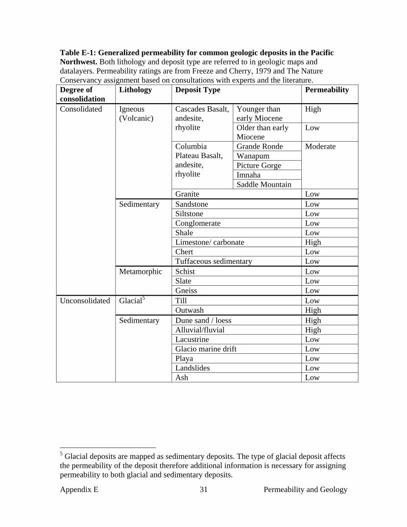
Appendix E 31 Permeability and Geology
Table E-1: Generalized permeability for common geologic deposits in the Pacific Northwest. Both lithology and deposit type are referred to in geologic maps and datalayers. Permeability ratings are from Freeze and Cherry, 1979 and The Nature Conservancy assignment based on consultations with experts and the literature. Degree of consolidation
Lithology Deposit Type Permeability
Younger than early Miocene
High Cascades Basalt, andesite, rhyolite Older than early
Miocene Low
Grande Ronde Wanapum Picture Gorge Imnaha
Columbia Plateau Basalt, andesite, rhyolite
Saddle Mountain
Moderate
Igneous (Volcanic)
Granite Low Sandstone Low Siltstone Low Conglomerate Low Shale Low Limestone/ carbonate High Chert Low
Sedimentary
Tuffaceous sedimentary Low Schist Low Slate Low
Consolidated
Metamorphic
Gneiss Low Till Low Glacial5 Outwash High Dune sand / loess High Alluvial/fluvial High Lacustrine Low Glacio marine drift Low Playa Low Landslides Low
Unconsolidated
Sedimentary
Ash Low
5 Glacial deposits are mapped as sedimentary deposits. The type of glacial deposit affects the permeability of the deposit therefore additional information is necessary for assigning permeability to both glacial and sedimentary deposits.
Appendix E 32 Permeability and Geology
Details of the permeability of surficial geologic deposits in the Pacific Northwest: The deposits of the Pacific Northwest can be classified as either consolidated or unconsolidated deposits. In general, consolidated deposits are less permeable than unconsolidated deposits, although there are some exceptions, and the presence of faults and fractures in the consolidated deposits can greatly increase their permeability. 1. Consolidated deposits: A. Igneous: i.. Volcanic
These deposits include volcanic or pyroclastic material such as basaltic, andesitic and rhyolitic vent deposits, volcaniclastic deposits and lava flows. Many of the lava flows have good lateral permeability at the top and base of individual flows but poor lateral permeability in the center of the deposit. The age of volcanic deposits of the PNW is important to determining their vertical permeability; the vertical fractures and cracks that produce high permeability in younger deposits are often filled with fine-grained materials in older deposits. As a result, older volcanic deposits generally have poor permeability. In the Pacific Northwest, the volcanic deposits of the High Cascades tend to be young (less than mid-Miocene in age; Table E-2) and of higher permeablility, while those of the western Cascades tend to be older and of lower permeability. Lavas of the Columbia Plateau tend to have moderate horizontal permeability and low vertical permeability.
ii. Other
Additionally, rocks such as granite are classified as igneous; however, these rocks are generally much less permeable unless they are fractured.
B. Sedimentary: These deposits include rocks that were originally deposited as individual sediment grains. These types of materials can form in a variety of environments. Those materials formed from marine and lake (lacustrine) deposits tend to have very low permeability. The permeability of individual deposits can be higher if fractures or faults are present.
C. Metamorphic:
Metamorphic rocks form when geologic deposits are subjected to high temperatures and pressures. In general these deposits have low permeability; however, locally they may transmit water if faults and fractures are present. Additionally, metamorphosed sedimentary deposits such as limestone or carbonate deposits can be fairly permeable.
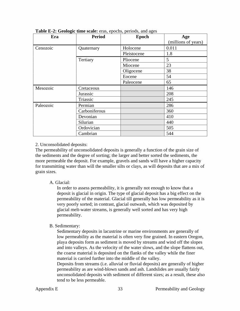
Appendix E 33 Permeability and Geology
Table E-2: Geologic time scale: eras, epochs, periods, and ages Era Period Epoch Age
(millions of years) Holocene 0.011 Quaternary Pleistocene 1.8 Pliocene 5 Miocene 23 Oligocene 38 Eocene 54
Cenozoic
Tertiary
Paleocene 65 Cretaceous 146 Jurassic 208
Mesozoic
Triassic 245 Permian 286 Carboniferous 360 Devonian 410 Silurian 440 Ordovician 505
Paleozoic
Cambrian 544 2. Unconsolidated deposits: The permeability of unconsolidated deposits is generally a function of the grain size of the sediments and the degree of sorting; the larger and better sorted the sediments, the more permeable the deposit. For example, gravels and sands will have a higher capacity for transmitting water than will the smaller silts or clays, as will deposits that are a mix of grain sizes. A. Glacial:
In order to assess permeability, it is generally not enough to know that a deposit is glacial in origin. The type of glacial deposit has a big effect on the permeability of the material. Glacial till generally has low permeability as it is very poorly sorted; in contrast, glacial outwash, which was deposited by glacial melt-water streams, is generally well sorted and has very high permeability.
B. Sedimentary:
Sedimentary deposits in lacustrine or marine environments are generally of low permeability as the material is often very fine grained. In eastern Oregon, playa deposits form as sediment is moved by streams and wind off the slopes and into valleys. As the velocity of the water slows, and the slope flattens out, the coarse material is deposited on the flanks of the valley while the finer material is carried further into the middle of the valley. Deposits from streams (i.e. alluvial or fluvial deposits) are generally of higher permeability as are wind-blown sands and ash. Landslides are usually fairly unconsolidated deposits with sediment of different sizes; as a result, these also tend to be less permeable.

Appendix E 34 Permeability and Geology
Interpreting the surficial geology datalayers: In the statewide surficial geology datalayer, geologic deposits are assigned map symbols (also termed ‘p types’ on the Oregon datalayer). These are a series of letters that correspond with a specific type of deposit ( http://www.gis.state.or.us/data/metadata/k500/GEOLGNDT.TXT.) The first capital letters of the map symbol usually refer to the geologic period in which the deposits were formed (Table E-3). The lower case letters that follow indicate something about the specific deposit – its type, a formation name, etc… The particular convention used for these small case letters varies by map product. Table E-3: Map symbol letters (capital letters) used to signify geologic periods
Geologic Period Map Symbol Letter Quaternary Q Tertiary T Cretaceous K Jurassic J Triassic TR
To aid users of the methods guide, an initial assignment of relative permeability (high or low) has been made to the map units in the statewide geology layer of Oregon (Walker and McLeod, 1991). These were made by a geologist, Wendy Gerstel (Table E-4), using the following approach:
1. Those map units with formation names were assigned relative permeability based on unit descriptions in the literature.
2. By overlaying the 1:500,000-scale mapping onto larger-scale geologic mapping (available for eastern Oregon from OGDMC) and using unit information from the larger-scale mapping, relative permeability was assigned to the 1:500,000-scale map units without formation names.
3. The remaining units, those with minimal descriptive date, were assigned relative permeability based on broad assumptions about the rock type indicated by the map unit symbol and name.
If more refined geologic maps are available, they should be used instead of the statewide data. It is important to have a geologist familiar with the local area review the permeability assignments in particular because some of the deposits mapped in this statewide datalayer are grouped into broad categories that are composed of multiple deposits with extremely variable permeabilities.
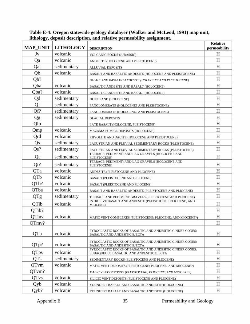
Appendix E 35 Permeability and Geology
Table E-4: Oregon statewide geology datalayer (Walker and McLeod, 1991) map unit, lithology, deposit description, and relative permeability assignment.
MAP_UNIT LITHOLOGY DESCRIPTION Relative
permeability Jv volcanic VOLCANIC ROCKS (JURASSIC) H Qa volcanic ANDESITE (HOLOCENE AND PLEISTOCENE) H Qal sedimentary ALLUVIAL DEPOSITS H Qb volcanic BASALT AND BASALTIC ANDESITE (HOLOCENE AND PLEISTOCENE) H Qb? BASALT AND BASALTIC ANDESITE (HOLOCENE AND PLEISTOCENE) H Qba volcanic BASALTIC ANDESITE AND BASALT (HOLOCENE) H Qba? volcanic BASALTIC ANDESITE AND BASALT (HOLOCENE) H Qd sedimentary DUNE SAND (HOLOCENE) H Qf sedimentary FANGLOMERATE (HOLOCENE? AND PLEISTOCENE) H Qf? sedimentary FANGLOMERATE (HOLOCENE? AND PLEISTOCENE) H Qg sedimentary GLACIAL DEPOSITS H Qlb LATE BASALT (HOLOCENE, PLEISTOCENE) H Qmp volcanic MAZAMA PUMICE DEPOSITS (HOLOCENE) H Qrd volcanic RHYOLITE AND DACITE (HOLOCENE AND PLEISTOCENE) H Qs sedimentary LACUSTRIAN AND FLUVIAL SEDIMENTARY ROCKS (PLEISTOCENE) H Qs? sedimentary LACUSTRIAN AND FLUVIAL SEDIMENTARY ROCKS (PLEISTOCENE) H Qt sedimentary
TERRACE; PEDIMENT; AND LAG GRAVELS (HOLOCENE AND PLEISTOCENE) H
Qt? sedimentary TERRACE; PEDIMENT; AND LAG GRAVELS (HOLOCENE AND PLEISTOCENE) H
QTa volcanic ANDESITE (PLEISTOCENE AND PLIOCENE) H QTb volcanic BASALT (PLEISTOCENE AND PLIOCENE) H QTb? volcanic BASALT (PLEISTOCENE AND PLIOCENE) H QTba volcanic BASALT AND BASALTIC ANDESITE (PLEISTOCENE AND PLIOCENE) H QTg sedimentary TERRACE AND PEDIMENT GRAVELS (PLEISTOCENE AND PLIOCENE) H QTib volcanic
INTRUSIVE BASALT AND ANDESITE (PLEISTOCENE, PLIOCENE, AND MIOCENE) H
QTib? H QTmv volcanic MAFIC VENT COMPLEXES (PLEISTOCENE; PLIOCENE; AND MIOCENE?) H QTmv? H
QTp volcanic PYROCLASTIC ROCKS OF BASALTIC AND ANDESITIC CINDER CONES: BASALTIC AND ANDESITIC EJECTA H
QTp? volcanic PYROCLASTIC ROCKS OF BASALTIC AND ANDESITIC CINDER CONES: BASALTIC AND ANDESITIC EJECTA H
QTps volcanic PYROCLASTIC ROCKS OF BASALTIC AND ANDESITIC CINDER CONES: SUBAQUEOUS BASALTIC AND ANDESITIC EJECTA H
QTs sedimentary SEDIMENTARY ROCKS (PLEISTOCENE AND PLIOCENE) H QTvm volcanic MAFIC VENT DEPOSITS (PLEISTOCENE; PLIOCENE; AND MIOCENE?) H QTvm? MAFIC VENT DEPOSITS (PLEISTOCENE; PLIOCENE; AND MIOCENE?) H QTvs volcanic SILICIC VENT DEPOSITS (PLEISTOCENE AND PLIOCENE) H Qyb volcanic YOUNGEST BASALT AND BASALTIC ANDESITE (HOLOCENE) H Qyb? volcanic YOUNGEST BASALT AND BASALTIC ANDESITE (HOLOCENE) H
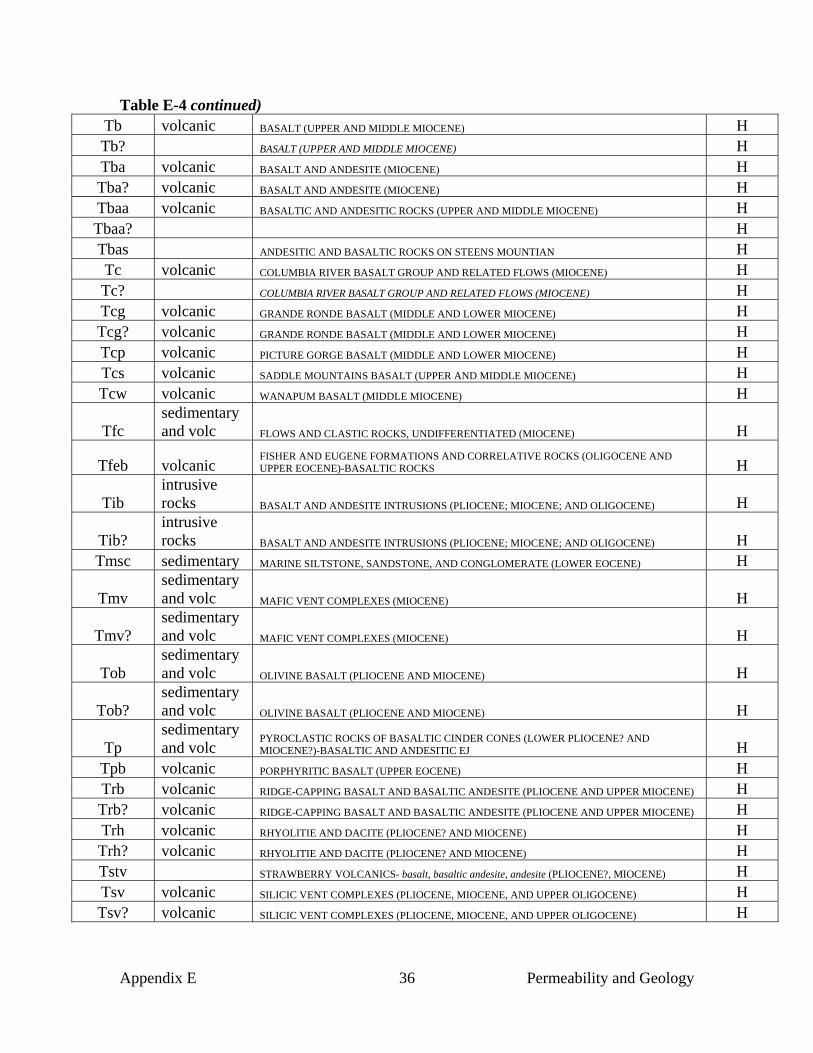
Appendix E 36 Permeability and Geology
Table E-4 continued) Tb volcanic BASALT (UPPER AND MIDDLE MIOCENE) H Tb? BASALT (UPPER AND MIDDLE MIOCENE) H Tba volcanic BASALT AND ANDESITE (MIOCENE) H Tba? volcanic BASALT AND ANDESITE (MIOCENE) H Tbaa volcanic BASALTIC AND ANDESITIC ROCKS (UPPER AND MIDDLE MIOCENE) H Tbaa? H Tbas ANDESITIC AND BASALTIC ROCKS ON STEENS MOUNTIAN H Tc volcanic COLUMBIA RIVER BASALT GROUP AND RELATED FLOWS (MIOCENE) H Tc? COLUMBIA RIVER BASALT GROUP AND RELATED FLOWS (MIOCENE) H Tcg volcanic GRANDE RONDE BASALT (MIDDLE AND LOWER MIOCENE) H Tcg? volcanic GRANDE RONDE BASALT (MIDDLE AND LOWER MIOCENE) H Tcp volcanic PICTURE GORGE BASALT (MIDDLE AND LOWER MIOCENE) H Tcs volcanic SADDLE MOUNTAINS BASALT (UPPER AND MIDDLE MIOCENE) H Tcw volcanic WANAPUM BASALT (MIDDLE MIOCENE) H
Tfc sedimentary and volc FLOWS AND CLASTIC ROCKS, UNDIFFERENTIATED (MIOCENE) H
Tfeb volcanic FISHER AND EUGENE FORMATIONS AND CORRELATIVE ROCKS (OLIGOCENE AND UPPER EOCENE)-BASALTIC ROCKS H
Tib intrusive rocks BASALT AND ANDESITE INTRUSIONS (PLIOCENE; MIOCENE; AND OLIGOCENE) H
Tib? intrusive rocks BASALT AND ANDESITE INTRUSIONS (PLIOCENE; MIOCENE; AND OLIGOCENE) H
Tmsc sedimentary MARINE SILTSTONE, SANDSTONE, AND CONGLOMERATE (LOWER EOCENE) H
Tmv sedimentary and volc MAFIC VENT COMPLEXES (MIOCENE) H
Tmv? sedimentary and volc MAFIC VENT COMPLEXES (MIOCENE) H
Tob sedimentary and volc OLIVINE BASALT (PLIOCENE AND MIOCENE) H
Tob? sedimentary and volc OLIVINE BASALT (PLIOCENE AND MIOCENE) H
Tp sedimentary and volc
PYROCLASTIC ROCKS OF BASALTIC CINDER CONES (LOWER PLIOCENE? AND MIOCENE?)-BASALTIC AND ANDESITIC EJ H
Tpb volcanic PORPHYRITIC BASALT (UPPER EOCENE) H Trb volcanic RIDGE-CAPPING BASALT AND BASALTIC ANDESITE (PLIOCENE AND UPPER MIOCENE) H Trb? volcanic RIDGE-CAPPING BASALT AND BASALTIC ANDESITE (PLIOCENE AND UPPER MIOCENE) H Trh volcanic RHYOLITIE AND DACITE (PLIOCENE? AND MIOCENE) H Trh? volcanic RHYOLITIE AND DACITE (PLIOCENE? AND MIOCENE) H Tstv STRAWBERRY VOLCANICS- basalt, basaltic andesite, andesite (PLIOCENE?, MIOCENE) H Tsv volcanic SILICIC VENT COMPLEXES (PLIOCENE, MIOCENE, AND UPPER OLIGOCENE) H Tsv? volcanic SILICIC VENT COMPLEXES (PLIOCENE, MIOCENE, AND UPPER OLIGOCENE) H
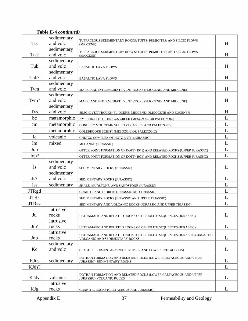
Appendix E 37 Permeability and Geology
Table E-4 continued)
Tts sedimentary and volc
TUFFACEOUS SEDIMENTARY ROKCS; TUFFS; PUMICITES; AND SILCIC FLOWS (MIOCENE) H
Tts? sedimentary and volc
TUFFACEOUS SEDIMENTARY ROKCS; TUFFS; PUMICITES; AND SILCIC FLOWS (MIOCENE) H
Tub sedimentary and volc BASALTIC LAVA FLOWS H
Tub? sedimentary and volc BASALTIC LAVA FLOWS H
Tvm sedimentary and volc MAFIC AND INTERMEDIATE VENT ROCKS (PLIOCENE? AND MIOCENE) H
Tvm? sedimentary and volc MAFIC AND INTERMEDIATE VENT ROCKS (PLIOCENE? AND MIOCENE) H
Tvs sedimentary and volc SILICIC VENT ROCKS (PLIOCENE; MIOCENE; OLIGOCENE AND EOCENE?) H
bc metamorphic AMPHIBOLITE OF BRIGGS CREEK (MESOZOIC OR PALEOZOIC) L cm metamorphic CONDREY MOUNTAIN SCHIST (TRIASSIC? AND PALEOZOIC?) L cs metamorphic COLEBROOKE SCHIST (MESOZOIC OR PALEOZOIC) L Jc volcanic CHETCO COMPLEX OF HOTZ (1971) (JURASSIC) L Jm mixed MELANGE (JURASSIC) L Jop OTTER POINT FORMATION OF DOTT (1971) AND RELATED ROCKS (UPPER JURASSIC) L Jop? OTTER POINT FORMATION OF DOTT (1971) AND RELATED ROCKS (UPPER JURASSIC) L
Js sedimentary and volc SEDIMENTARY ROCKS (JURASSIC) L
Js? sedimentary and volc SEDIMENTARY ROCKS (JURASSIC) L
Jss sedimentary SHALE, MUDSTONE, AND SANDSTONE (JURASSIC) L JTRgd GRANITE AND DIORITE (JURASSIC AND TRIASSIC L JTRs SEDIMENTARY ROCKS (JURASSIC AND UPPER TRIASSIC) L JTRsv SEDIMENTARY AND VOLCANIC ROCKS (JURASSIC AND UPPER TRIASSIC) L
Ju intrusive rocks ULTRAMAFIC AND RELATED ROCKS OF OPHIOLITE SEQUENCES (JURASSIC) L
Ju? intrusive rocks ULTRAMAFIC AND RELATED ROCKS OF OPHIOLITE SEQUENCES (JURASSIC) L
Jub intrusive rocks
ULTRAMAFIC AND RELATED ROCKS OF OPHIOLITE SEQUENCES (JURASSIC)-BASALTIC VOLCANIC AND SEDIMENTARY ROCKS L
Kc sedimentary and volc CLASTIC SEDIMENTARY ROCKS (UPPER AND LOWER CRETACEOUS) L
KJds sedimentary DOTHAN FORMATION AND RELATED ROCKS (LOWER CRETACEOUS AND UPPER JURASSIC)-SEDIMENTARY ROCKS L
KJds? L
KJdv volcanic DOTHAN FORMATION AND RELATED ROCKS (LOWER CRETACEOUS AND UPPER JURASSIC)-VOLCANIC ROCKS L
KJg intrusive rocks GRANITIC ROCKS (CRETACEOUS AND JURASSIC) L
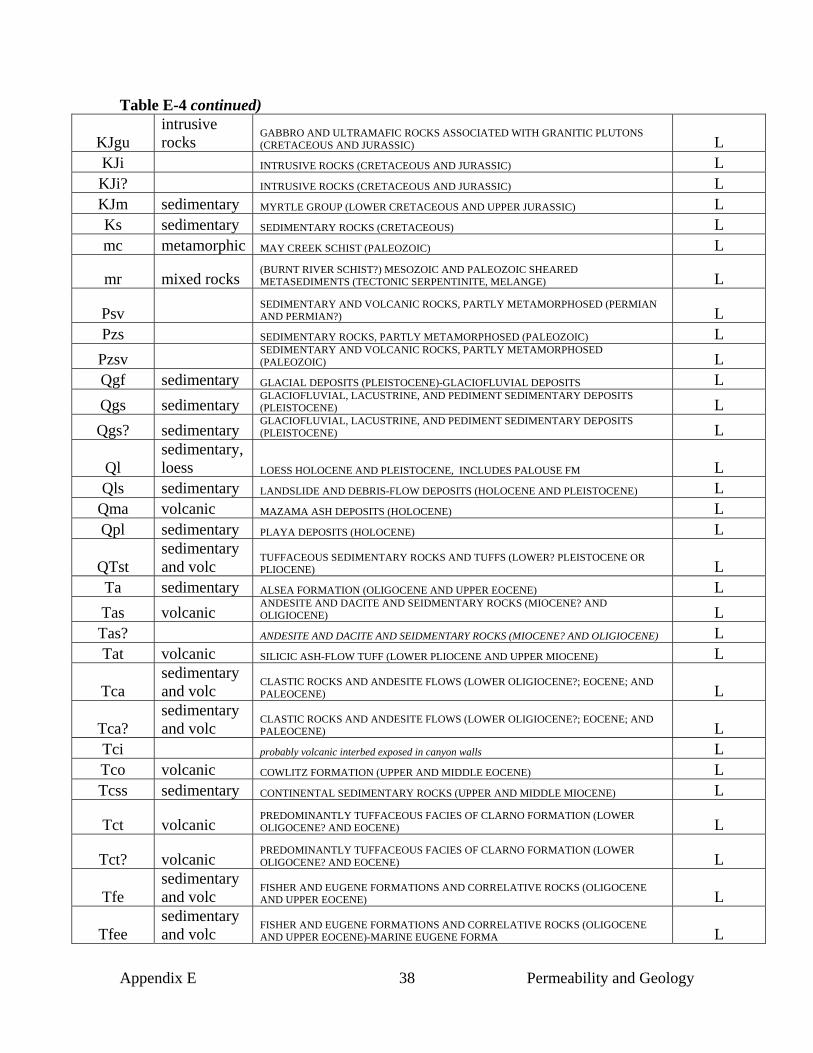
Appendix E 38 Permeability and Geology
Table E-4 continued)
KJgu intrusive rocks
GABBRO AND ULTRAMAFIC ROCKS ASSOCIATED WITH GRANITIC PLUTONS (CRETACEOUS AND JURASSIC) L
KJi INTRUSIVE ROCKS (CRETACEOUS AND JURASSIC) L KJi? INTRUSIVE ROCKS (CRETACEOUS AND JURASSIC) L KJm sedimentary MYRTLE GROUP (LOWER CRETACEOUS AND UPPER JURASSIC) L Ks sedimentary SEDIMENTARY ROCKS (CRETACEOUS) L mc metamorphic MAY CREEK SCHIST (PALEOZOIC) L
mr mixed rocks (BURNT RIVER SCHIST?) MESOZOIC AND PALEOZOIC SHEARED METASEDIMENTS (TECTONIC SERPENTINITE, MELANGE) L
Psv SEDIMENTARY AND VOLCANIC ROCKS, PARTLY METAMORPHOSED (PERMIAN AND PERMIAN?) L
Pzs SEDIMENTARY ROCKS, PARTLY METAMORPHOSED (PALEOZOIC) L Pzsv
SEDIMENTARY AND VOLCANIC ROCKS, PARTLY METAMORPHOSED (PALEOZOIC) L
Qgf sedimentary GLACIAL DEPOSITS (PLEISTOCENE)-GLACIOFLUVIAL DEPOSITS L Qgs sedimentary
GLACIOFLUVIAL, LACUSTRINE, AND PEDIMENT SEDIMENTARY DEPOSITS (PLEISTOCENE) L
Qgs? sedimentary GLACIOFLUVIAL, LACUSTRINE, AND PEDIMENT SEDIMENTARY DEPOSITS (PLEISTOCENE) L
Ql sedimentary, loess LOESS HOLOCENE AND PLEISTOCENE, INCLUDES PALOUSE FM L
Qls sedimentary LANDSLIDE AND DEBRIS-FLOW DEPOSITS (HOLOCENE AND PLEISTOCENE) L Qma volcanic MAZAMA ASH DEPOSITS (HOLOCENE) L Qpl sedimentary PLAYA DEPOSITS (HOLOCENE) L
QTst sedimentary and volc
TUFFACEOUS SEDIMENTARY ROCKS AND TUFFS (LOWER? PLEISTOCENE OR PLIOCENE) L
Ta sedimentary ALSEA FORMATION (OLIGOCENE AND UPPER EOCENE) L Tas volcanic
ANDESITE AND DACITE AND SEIDMENTARY ROCKS (MIOCENE? AND OLIGIOCENE) L
Tas? ANDESITE AND DACITE AND SEIDMENTARY ROCKS (MIOCENE? AND OLIGIOCENE) L Tat volcanic SILICIC ASH-FLOW TUFF (LOWER PLIOCENE AND UPPER MIOCENE) L
Tca sedimentary and volc
CLASTIC ROCKS AND ANDESITE FLOWS (LOWER OLIGIOCENE?; EOCENE; AND PALEOCENE) L
Tca? sedimentary and volc
CLASTIC ROCKS AND ANDESITE FLOWS (LOWER OLIGIOCENE?; EOCENE; AND PALEOCENE) L
Tci probably volcanic interbed exposed in canyon walls L Tco volcanic COWLITZ FORMATION (UPPER AND MIDDLE EOCENE) L Tcss sedimentary CONTINENTAL SEDIMENTARY ROCKS (UPPER AND MIDDLE MIOCENE) L
Tct volcanic PREDOMINANTLY TUFFACEOUS FACIES OF CLARNO FORMATION (LOWER OLIGOCENE? AND EOCENE) L
Tct? volcanic PREDOMINANTLY TUFFACEOUS FACIES OF CLARNO FORMATION (LOWER OLIGOCENE? AND EOCENE) L
Tfe sedimentary and volc
FISHER AND EUGENE FORMATIONS AND CORRELATIVE ROCKS (OLIGOCENE AND UPPER EOCENE) L
Tfee sedimentary and volc
FISHER AND EUGENE FORMATIONS AND CORRELATIVE ROCKS (OLIGOCENE AND UPPER EOCENE)-MARINE EUGENE FORMA L
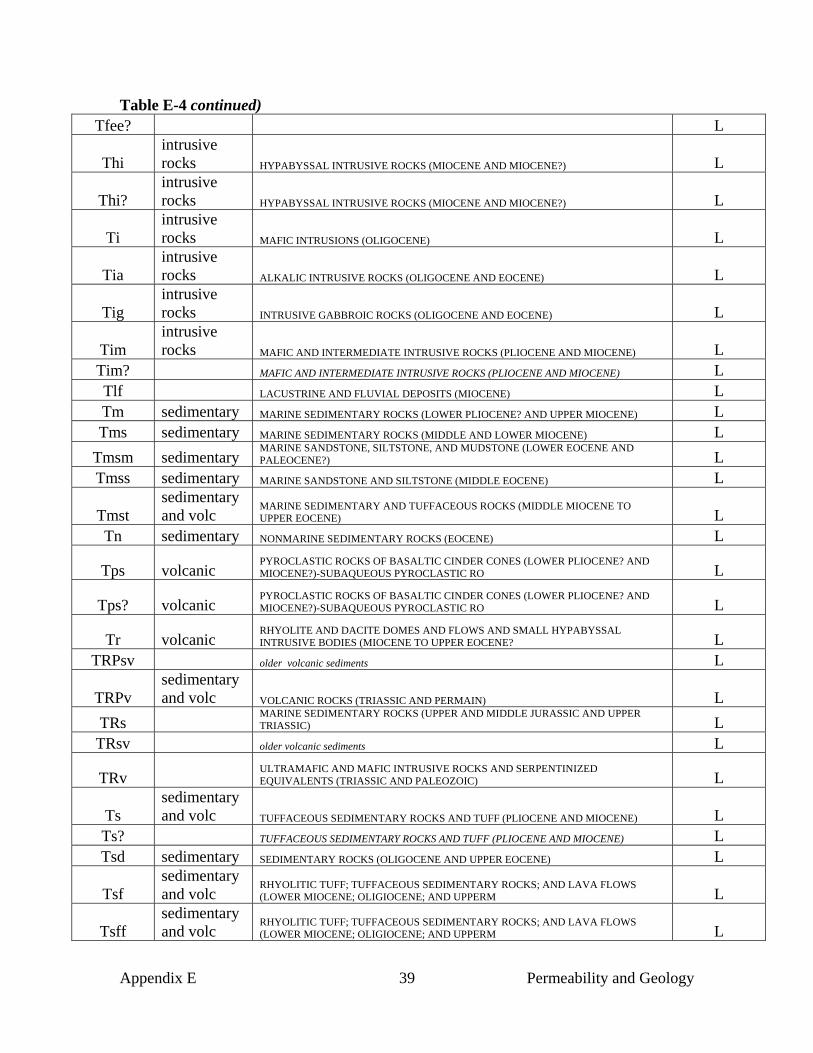
Appendix E 39 Permeability and Geology
Table E-4 continued) Tfee? L
Thi intrusive rocks HYPABYSSAL INTRUSIVE ROCKS (MIOCENE AND MIOCENE?) L
Thi? intrusive rocks HYPABYSSAL INTRUSIVE ROCKS (MIOCENE AND MIOCENE?) L
Ti intrusive rocks MAFIC INTRUSIONS (OLIGOCENE) L
Tia intrusive rocks ALKALIC INTRUSIVE ROCKS (OLIGOCENE AND EOCENE) L
Tig intrusive rocks INTRUSIVE GABBROIC ROCKS (OLIGOCENE AND EOCENE) L
Tim intrusive rocks MAFIC AND INTERMEDIATE INTRUSIVE ROCKS (PLIOCENE AND MIOCENE) L
Tim? MAFIC AND INTERMEDIATE INTRUSIVE ROCKS (PLIOCENE AND MIOCENE) L Tlf LACUSTRINE AND FLUVIAL DEPOSITS (MIOCENE) L Tm sedimentary MARINE SEDIMENTARY ROCKS (LOWER PLIOCENE? AND UPPER MIOCENE) L Tms sedimentary MARINE SEDIMENTARY ROCKS (MIDDLE AND LOWER MIOCENE) L
Tmsm sedimentary MARINE SANDSTONE, SILTSTONE, AND MUDSTONE (LOWER EOCENE AND PALEOCENE?) L
Tmss sedimentary MARINE SANDSTONE AND SILTSTONE (MIDDLE EOCENE) L
Tmst sedimentary and volc
MARINE SEDIMENTARY AND TUFFACEOUS ROCKS (MIDDLE MIOCENE TO UPPER EOCENE) L
Tn sedimentary NONMARINE SEDIMENTARY ROCKS (EOCENE) L
Tps volcanic PYROCLASTIC ROCKS OF BASALTIC CINDER CONES (LOWER PLIOCENE? AND MIOCENE?)-SUBAQUEOUS PYROCLASTIC RO L
Tps? volcanic PYROCLASTIC ROCKS OF BASALTIC CINDER CONES (LOWER PLIOCENE? AND MIOCENE?)-SUBAQUEOUS PYROCLASTIC RO L
Tr volcanic RHYOLITE AND DACITE DOMES AND FLOWS AND SMALL HYPABYSSAL INTRUSIVE BODIES (MIOCENE TO UPPER EOCENE? L
TRPsv older volcanic sediments L
TRPv sedimentary and volc VOLCANIC ROCKS (TRIASSIC AND PERMAIN) L
TRs MARINE SEDIMENTARY ROCKS (UPPER AND MIDDLE JURASSIC AND UPPER TRIASSIC) L
TRsv older volcanic sediments L
TRv ULTRAMAFIC AND MAFIC INTRUSIVE ROCKS AND SERPENTINIZED EQUIVALENTS (TRIASSIC AND PALEOZOIC) L
Ts sedimentary and volc TUFFACEOUS SEDIMENTARY ROCKS AND TUFF (PLIOCENE AND MIOCENE) L
Ts? TUFFACEOUS SEDIMENTARY ROCKS AND TUFF (PLIOCENE AND MIOCENE) L Tsd sedimentary SEDIMENTARY ROCKS (OLIGOCENE AND UPPER EOCENE) L
Tsf sedimentary and volc
RHYOLITIC TUFF; TUFFACEOUS SEDIMENTARY ROCKS; AND LAVA FLOWS (LOWER MIOCENE; OLIGIOCENE; AND UPPERM L
Tsff sedimentary and volc
RHYOLITIC TUFF; TUFFACEOUS SEDIMENTARY ROCKS; AND LAVA FLOWS (LOWER MIOCENE; OLIGIOCENE; AND UPPERM L
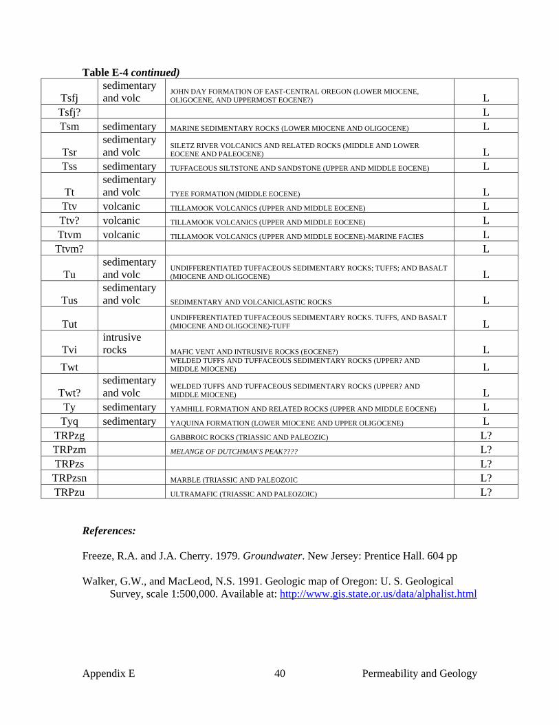
Appendix E 40 Permeability and Geology
Table E-4 continued)
Tsfj sedimentary and volc
JOHN DAY FORMATION OF EAST-CENTRAL OREGON (LOWER MIOCENE, OLIGOCENE, AND UPPERMOST EOCENE?) L
Tsfj? L Tsm sedimentary MARINE SEDIMENTARY ROCKS (LOWER MIOCENE AND OLIGOCENE) L
Tsr sedimentary and volc
SILETZ RIVER VOLCANICS AND RELATED ROCKS (MIDDLE AND LOWER EOCENE AND PALEOCENE) L
Tss sedimentary TUFFACEOUS SILTSTONE AND SANDSTONE (UPPER AND MIDDLE EOCENE) L
Tt sedimentary and volc TYEE FORMATION (MIDDLE EOCENE) L
Ttv volcanic TILLAMOOK VOLCANICS (UPPER AND MIDDLE EOCENE) L Ttv? volcanic TILLAMOOK VOLCANICS (UPPER AND MIDDLE EOCENE) L Ttvm volcanic TILLAMOOK VOLCANICS (UPPER AND MIDDLE EOCENE)-MARINE FACIES L Ttvm? L
Tu sedimentary and volc
UNDIFFERENTIATED TUFFACEOUS SEDIMENTARY ROCKS; TUFFS; AND BASALT (MIOCENE AND OLIGOCENE) L
Tus sedimentary and volc SEDIMENTARY AND VOLCANICLASTIC ROCKS L
Tut UNDIFFERENTIATED TUFFACEOUS SEDIMENTARY ROCKS. TUFFS, AND BASALT (MIOCENE AND OLIGOCENE)-TUFF L
Tvi intrusive rocks MAFIC VENT AND INTRUSIVE ROCKS (EOCENE?) L
Twt WELDED TUFFS AND TUFFACEOUS SEDIMENTARY ROCKS (UPPER? AND MIDDLE MIOCENE) L
Twt? sedimentary and volc
WELDED TUFFS AND TUFFACEOUS SEDIMENTARY ROCKS (UPPER? AND MIDDLE MIOCENE) L
Ty sedimentary YAMHILL FORMATION AND RELATED ROCKS (UPPER AND MIDDLE EOCENE) L Tyq sedimentary YAQUINA FORMATION (LOWER MIOCENE AND UPPER OLIGOCENE) L
TRPzg GABBROIC ROCKS (TRIASSIC AND PALEOZIC) L? TRPzm MELANGE OF DUTCHMAN'S PEAK???? L? TRPzs L? TRPzsn MARBLE (TRIASSIC AND PALEOZOIC L? TRPzu ULTRAMAFIC (TRIASSIC AND PALEOZOIC) L?
References: Freeze, R.A. and J.A. Cherry. 1979. Groundwater. New Jersey: Prentice Hall. 604 pp Walker, G.W., and MacLeod, N.S. 1991. Geologic map of Oregon: U. S. Geological
Survey, scale 1:500,000. Available at: http://www.gis.state.or.us/data/alphalist.html
Appendix F:Key Ecological Attributes & Indicators Introduction 41
APPENDIX F: KEAS AND INDICATORS FOR GROUNDWATER-DEPENDENT SPECIES This appendix provides further details on the key ecological attributes (KEAs) and indicators for two groundwater-dependent species: bull trout and springsnails. References are at the end of this appendix.
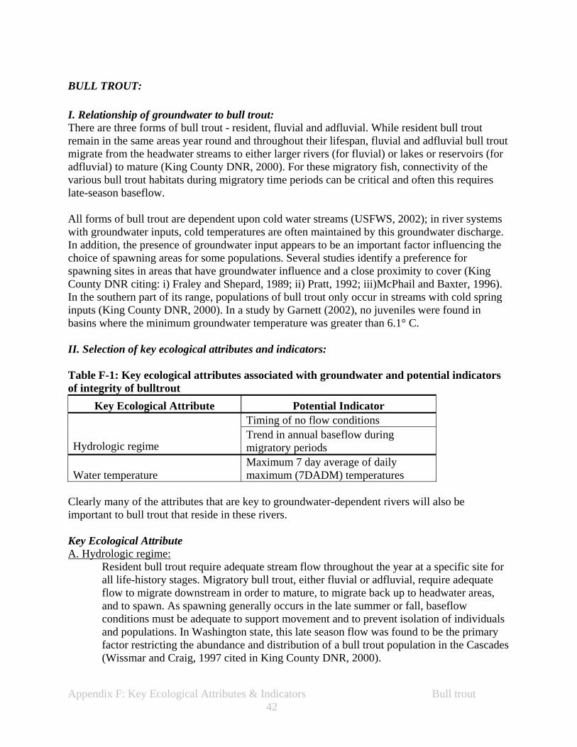
Appendix F: Key Ecological Attributes & Indicators Bull trout 42
BULL TROUT: I. Relationship of groundwater to bull trout: There are three forms of bull trout - resident, fluvial and adfluvial. While resident bull trout remain in the same areas year round and throughout their lifespan, fluvial and adfluvial bull trout migrate from the headwater streams to either larger rivers (for fluvial) or lakes or reservoirs (for adfluvial) to mature (King County DNR, 2000). For these migratory fish, connectivity of the various bull trout habitats during migratory time periods can be critical and often this requires late-season baseflow. All forms of bull trout are dependent upon cold water streams (USFWS, 2002); in river systems with groundwater inputs, cold temperatures are often maintained by this groundwater discharge. In addition, the presence of groundwater input appears to be an important factor influencing the choice of spawning areas for some populations. Several studies identify a preference for spawning sites in areas that have groundwater influence and a close proximity to cover (King County DNR citing: i) Fraley and Shepard, 1989; ii) Pratt, 1992; iii)McPhail and Baxter, 1996). In the southern part of its range, populations of bull trout only occur in streams with cold spring inputs (King County DNR, 2000). In a study by Garnett (2002), no juveniles were found in basins where the minimum groundwater temperature was greater than 6.1° C. II. Selection of key ecological attributes and indicators: Table F-1: Key ecological attributes associated with groundwater and potential indicators of integrity of bulltrout
Key Ecological Attribute Potential Indicator Timing of no flow conditions
Hydrologic regime Trend in annual baseflow during migratory periods
Water temperature Maximum 7 day average of daily maximum (7DADM) temperatures
Clearly many of the attributes that are key to groundwater-dependent rivers will also be important to bull trout that reside in these rivers. Key Ecological Attribute A. Hydrologic regime:
Resident bull trout require adequate stream flow throughout the year at a specific site for all life-history stages. Migratory bull trout, either fluvial or adfluvial, require adequate flow to migrate downstream in order to mature, to migrate back up to headwater areas, and to spawn. As spawning generally occurs in the late summer or fall, baseflow conditions must be adequate to support movement and to prevent isolation of individuals and populations. In Washington state, this late season flow was found to be the primary factor restricting the abundance and distribution of a bull trout population in the Cascades (Wissmar and Craig, 1997 cited in King County DNR, 2000).
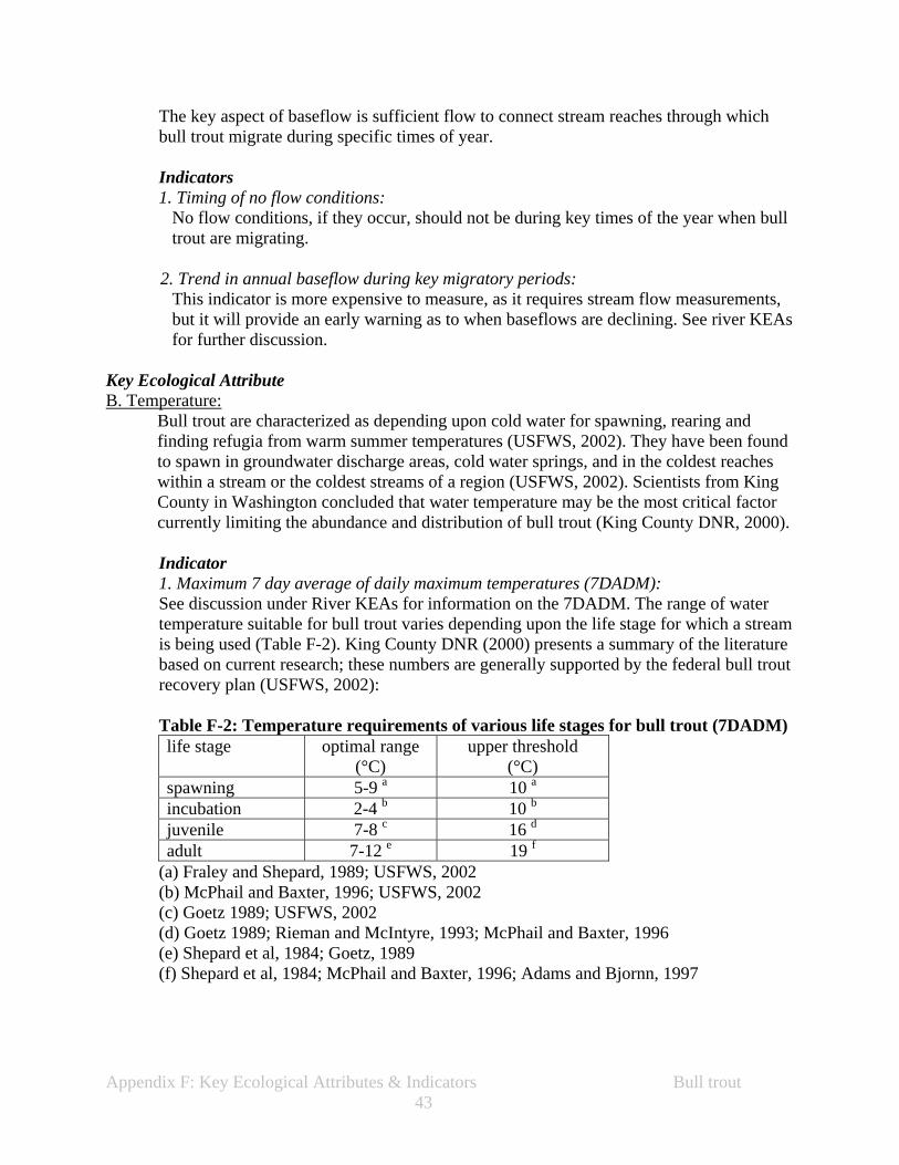
Appendix F: Key Ecological Attributes & Indicators Bull trout 43
The key aspect of baseflow is sufficient flow to connect stream reaches through which bull trout migrate during specific times of year. Indicators 1. Timing of no flow conditions:
No flow conditions, if they occur, should not be during key times of the year when bull trout are migrating.
2. Trend in annual baseflow during key migratory periods: This indicator is more expensive to measure, as it requires stream flow measurements, but it will provide an early warning as to when baseflows are declining. See river KEAs for further discussion.
Key Ecological Attribute B. Temperature:
Bull trout are characterized as depending upon cold water for spawning, rearing and finding refugia from warm summer temperatures (USFWS, 2002). They have been found to spawn in groundwater discharge areas, cold water springs, and in the coldest reaches within a stream or the coldest streams of a region (USFWS, 2002). Scientists from King County in Washington concluded that water temperature may be the most critical factor currently limiting the abundance and distribution of bull trout (King County DNR, 2000).
Indicator 1. Maximum 7 day average of daily maximum temperatures (7DADM): See discussion under River KEAs for information on the 7DADM. The range of water temperature suitable for bull trout varies depending upon the life stage for which a stream is being used (Table F-2). King County DNR (2000) presents a summary of the literature based on current research; these numbers are generally supported by the federal bull trout recovery plan (USFWS, 2002): Table F-2: Temperature requirements of various life stages for bull trout (7DADM) life stage optimal range
(°C) upper threshold
(°C) spawning 5-9 a 10 a incubation 2-4 b 10 b juvenile 7-8 c 16 d adult 7-12 e 19 f
(a) Fraley and Shepard, 1989; USFWS, 2002 (b) McPhail and Baxter, 1996; USFWS, 2002 (c) Goetz 1989; USFWS, 2002 (d) Goetz 1989; Rieman and McIntyre, 1993; McPhail and Baxter, 1996 (e) Shepard et al, 1984; Goetz, 1989 (f) Shepard et al, 1984; McPhail and Baxter, 1996; Adams and Bjornn, 1997
Appendix F: Key Ecological Attributes & Indicators Bull trout 44
III. Example: KEA and indicator identification for bull trout Bull trout are found in rivers of the western Cascades dependent upon groundwater. Both the fluvial and resident forms of the fish occur in this portion of the river. The fish migrate upriver to spawn during September and October; after emerging, they mature in the headwater areas of the watershed for two to three years before migrating downriver in the spring. In order to ensure connectivity of the downstream reaches of the stream with the headwater spawning areas for the fluvial fish, a primary KEA for this bull trout population is the hydrologic regime. It is critical that the groundwater flow between the downriver and headwater areas is adequate during September and October. An indicator of this would be the absence of no-flow conditions during September and October on these river reaches. This could be monitored by a biweekly visual inspection of flow conditions. A second KEA for these bull trout is temperature. Using the data presented in Table F-2, the indicator can be the maximum 7-day average of daily maximum temperatures in the specific reaches of river being used at a particular time of year. Stream temperatures can be measured with a recording temperature sensor placed in key locations in the stream. Desired conditions are:
• Maximum 7-day average of daily maximum temperature in the headwater reaches used for spawning does not exceed 9° C during September and October.
• Maximum 7-day average of daily maximum temperature in these headwater reaches does not exceed 8° C in key thermal refugia at any time of the year.
• Maximum 7-day average of daily maximum temperature in the downriver areas used by the bull trout does not exceed 12° C in key thermal refugia at any time of the year.
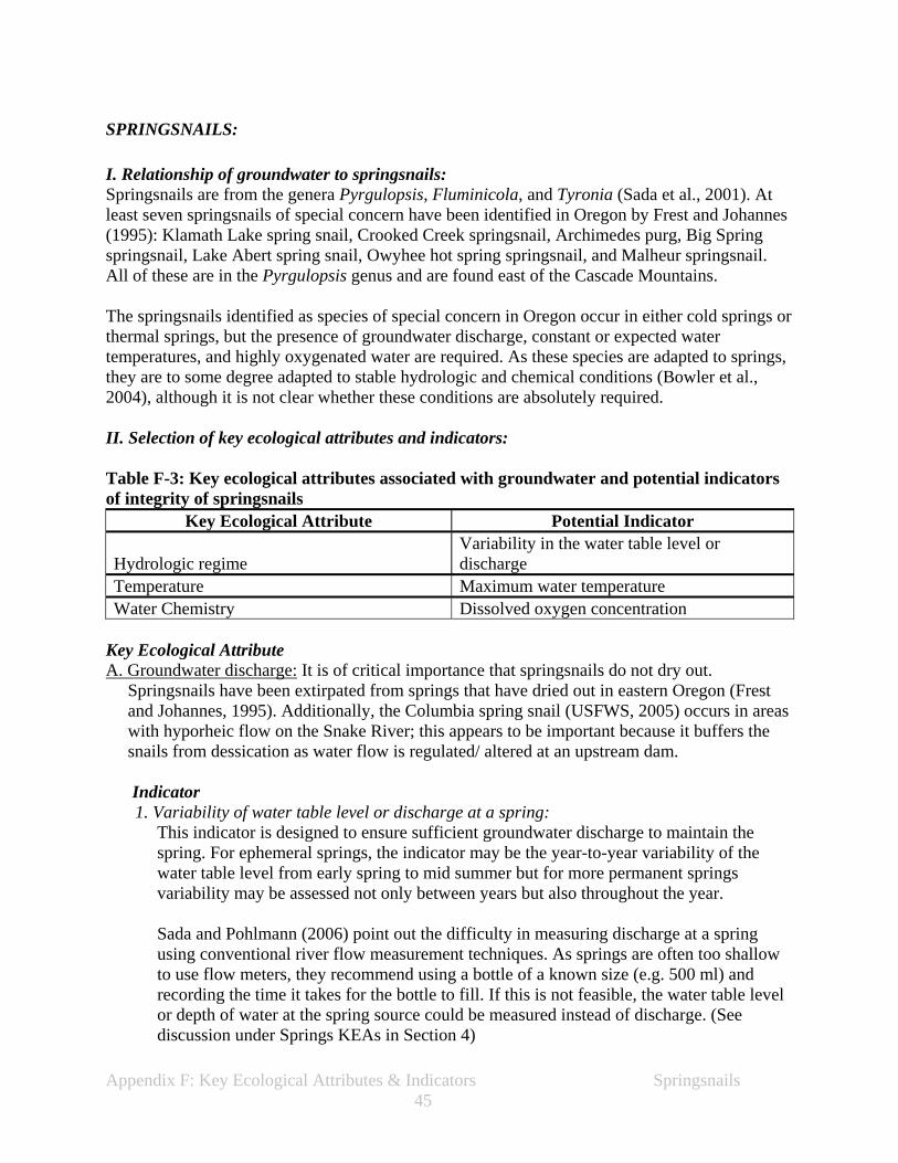
Appendix F: Key Ecological Attributes & Indicators Springsnails 45
SPRINGSNAILS: I. Relationship of groundwater to springsnails: Springsnails are from the genera Pyrgulopsis, Fluminicola, and Tyronia (Sada et al., 2001). At least seven springsnails of special concern have been identified in Oregon by Frest and Johannes (1995): Klamath Lake spring snail, Crooked Creek springsnail, Archimedes purg, Big Spring springsnail, Lake Abert spring snail, Owyhee hot spring springsnail, and Malheur springsnail. All of these are in the Pyrgulopsis genus and are found east of the Cascade Mountains. The springsnails identified as species of special concern in Oregon occur in either cold springs or thermal springs, but the presence of groundwater discharge, constant or expected water temperatures, and highly oxygenated water are required. As these species are adapted to springs, they are to some degree adapted to stable hydrologic and chemical conditions (Bowler et al., 2004), although it is not clear whether these conditions are absolutely required. II. Selection of key ecological attributes and indicators: Table F-3: Key ecological attributes associated with groundwater and potential indicators of integrity of springsnails
Key Ecological Attribute Potential Indicator
Hydrologic regime Variability in the water table level or discharge
Temperature Maximum water temperature Water Chemistry Dissolved oxygen concentration
Key Ecological Attribute A. Groundwater discharge: It is of critical importance that springsnails do not dry out.
Springsnails have been extirpated from springs that have dried out in eastern Oregon (Frest and Johannes, 1995). Additionally, the Columbia spring snail (USFWS, 2005) occurs in areas with hyporheic flow on the Snake River; this appears to be important because it buffers the snails from dessication as water flow is regulated/ altered at an upstream dam. Indicator 1. Variability of water table level or discharge at a spring:
This indicator is designed to ensure sufficient groundwater discharge to maintain the spring. For ephemeral springs, the indicator may be the year-to-year variability of the water table level from early spring to mid summer but for more permanent springs variability may be assessed not only between years but also throughout the year. Sada and Pohlmann (2006) point out the difficulty in measuring discharge at a spring using conventional river flow measurement techniques. As springs are often too shallow to use flow meters, they recommend using a bottle of a known size (e.g. 500 ml) and recording the time it takes for the bottle to fill. If this is not feasible, the water table level or depth of water at the spring source could be measured instead of discharge. (See discussion under Springs KEAs in Section 4)
Appendix F: Key Ecological Attributes & Indicators Springsnails 46
Key Ecological Attribute B. Temperature:
Indicator 1. Maximum water temperature: The critical temperature tolerated by springsnails will depend upon the species and its location. Many springsnails depend upon cold waters but some, such as the Harney Lake springsnail, occur in thermal springs and can tolerate higher temperatures (Bowler et al, 2004).
Key Ecological Attribute C. Water chemistry:
Indicator 1. Dissolved oxygen concentrations: Many sources suggest the dependence of springsnails on good water quality (Sada et al., 2001; USFWS, 2005; Bowler et al., 2004). Most of these references indicate that flowing water with adequate levels of oxygen is the critical factor. For Pyrgulopsis robusta, a threshold for dissolved oxygen of more than 5 mg/l has been established (USFWS, 2005).
Appendix F: Key Ecological Attributes & Indicators Springsnails 47
REFERENCES Adams, S.B., and T.C. Bjornn. 1997. Bull trout distributions related to temperature
regimes in four central Idaho streams. Pages 371-380 In: Mackay, W.C., M.K. Brewin, and M. Monita(eds.). Friends of the bull trout conference proceedings. Bull Trout Task Force (Alberta), c/o Trout Unlimited Canada, Calgary.
Bowler, P., Biodiversity Conservation Alliance, Center for Biological Diversity, Center
for Native Ecosystems, Western Watersheds Project, and The Xerces Society. 2004. Petition to list the Jackson Lake springsnail (Pyrgulopsis robusta), Harney Lake springsnail (Pyrgulopsis hendersoni), and Columbia springsnail (Pyrgulopsis new species 6) as threatened or endangered. Petition Before the Secretary of Interior. July 29, 2004.
Fraley, J.J., and B.B. Shepard. 1989. Life history, ecology, and population status of
migratory bull trout (Salvelinus confluentus) in the Flathead Lake and river system, Montana. Northwest Science 63:133-143.
Frest, T.J. and E.J. Johannes. 1995. Interior Columbia Basin mollusk species of special
concern. Final Report by Deixis Consultants. 284 pp. Garnett, B. L. 2002. The relationship between water temperature and bull trout
distribution and abundance. MS Thesis Fisheries and Wildlife. Utah State University. 94 pp.
Goetz, F. 1989. Biology of bull trout (Salvelinus confluentus): a literature review.
Willamette National Forest, Eugene, Oregon. 53 p. King County Department of Natural Resources. 2000. Literature Review and
Recommended Sampling Protocol for Bull Trout in King County. Seattle, WA. June 2000. Available at: http://dnr.metrokc.gov/stock/pdf/docs/wlr/BullTrtWhtPP/BullTrWP.pdf
McPhail, J.D., and J.S. Baxter. 1996. A review of bull trout (Salvelinus confluentus) life-
history and habitat use in relation to compensation and improvement opportunities. British Columbia Ministry of Environment, Lands and Parks. Fisheries Management Report No. 104. 35 p.
Pratt, K.L. 1992. A review of bull trout life history. Pages 5-9 In: Howell, P.J., and D.V.
Buchanan (eds.). Proceedings of the Gearhart Mountain bull trout workshop. Oregon Chapter of the American Fisheries Society, Corvallis.
Rieman, B.E., and J.D. McIntyre. 1993. Demographic and habitat requirements for
conservation of bull trout. U.S. Dept. of Agriculture, Forest Service. Intermountain Research Station, Ogden, Utah. Gen. Tech. Rep. INT-302. 38 p.
Appendix F: Key Ecological Attributes & Indicators Springsnails 48
Sada, D.W and K.F. Pohlmann. 2006. Draft U.S. National Park Service Mojave Inventory and Monitoring Network Spring Survey Protocols: Level I and Level II. February 1, 2006.
Sada, D.W., J.E. Williams, J.C. Silvey, A. Halford, J. Ramakka, P. Summers, and L.Lewis. 2001. Riparian Area Management: A guide to managing, restoring and conserving springs in the Western United States. Technical reference 1737-17. Bureau of Land Management, Denver Colorado. BLM/ST/ST-01/--1+1737. 70 pp.
Shepard, B., K.L. Pratt, and P. Graham. 1984. Life history of westslope cutthroat trout
and bull trout in the upper Flathead River basin, Montana. Montana Dept. of Fish, Wildlife, and Parks.
USFWS. 2002. Bull Trout (Salvelinus confluentus)Recovery Plan. October 2002.
Available at: http://www.fws.gov/pacific/bulltrout/colkla/recovery/ USFWS. 2005. Draft Best Available Biological Information for Four Petitioned
springsnails in Idaho, Oregon, Washington and Wyoming. Snake River Fish and Widlife Office, Boise Idaho. August 2005. 82 pp.
Wissmar, R.C., and S. Craig. 1997. Bull trout spawning Activity, Gold Creek,
Washington. Univ. of Washington, Fisheries Research Institute, Seattle. FRI-UW-9701. 15 p.
Appendix G 49 Glossary
APPENDIX G: GLOSSARY Aquifer –a geologic formation, group of formations, or part of a formation that contains sufficient saturated permeable material to yield significant quantities of water to springs and wells (USGS, 1996) Aquitard- geologic deposit that does not easily transmit water Baseflow – the sustained low flow of a stream, usually the ground-water inflow to a stream channel (USGS, 1996) Capillary fringe – The capillary fringe is the zone immediately above the water table in which all or some of the interstices in the soil are filled with water that is under less than atmospheric pressure and that is continuous with the water below the water table. The water is held in the voids by forces such as surface tension. (Lohman et al., 1972) Confined aquifer – aquifer in which groundwater is sandwiched between two aquitards Contributing area - area in a drainage basin that contributes water to stream flow or recharge to an aquifer (USGS, 1996) Desired future conditions (DFCs) – measurable objective for each indicator of a key ecological attribute (KEA). These form the basis of an adaptive management and monitoring program to measure the effectiveness of conservation strategies. Ephemeral streams – a stream or part of a stream that flows in direct response to precipitation; it receives little or no water from springs, melting snow or other sources; its channel is at all times above the water table (USGS, 1996). Groundwater – in the broader sense, all subsurface water (USGS, 1996); water that occurs below the ground surface, in cracks in rocks or in spaces between soil particles that are fully saturated (full of water not air) (Freeze and Cherry, 1979). Groundwater-dependent ecosystems (GDEs) – any ecosystem or species that must have access to groundwater to persist and to retain its ecological structure and function (Murray et al., 2006). Hydraulic head – pressure or elevation of groundwater Hydraulic redistribution – active movement of water by plant roots from one position in the soil profile to another; originally termed hydraulic lift as deep roots moved groundwater to the surface at night. Hydric soils – soil that is wet long enough to periodically produce anaerobic conditions (USGS, 1996)
Appendix G 50 Glossary
Hydrogeologic cross section – representative drawings of vertical and horizontal groundwater flow paths, topography and geologic deposits (hydrogeologic units) along specific transects in the contributing area Hydrogeologic setting – position of ecosystem (i.e. river, lake or wetland) in a watershed and the surrounding topography, soils, geology and climate Hydrogeology – the part of the study of hydrology that deals with the distribution and movement of groundwater in the soil and rocks of the Earth's crust Hydrograph – graph or record of water levels or flows throughout time Hydrologic regime – quantity, timing and duration of water delivery Hydroperiod – duration of inundation in a wetland Indicators – measurable parameters that indicate the condition of key ecological attributes (KEAs). These are the parameters measured in a monitoring program. Intermittent streams – streams that flow only when they receive water from rainfall runoff or springs, or from some surface source such as melting snow (USGS, 1996) Isohyetals – contour lines of equal precipitation Key ecological attributes (KEAs) – factors that are essential to defining or determining the integrity of a particular ecosystem or species. For GDEs, KEAs are usually 1) hydrologic regime, 2) water chemistry regime, and 3) temperature regime. Perennial streams – a stream that normally has water in its channel at all times (USGS, 1996) Phreatophyte – plant that uses groundwater that is near the surface Unconfined aquifer – an aquifer whose upper surface is free to fluctuate under atmospheric pressure (USGS, 1996); groundwater in geologic deposits in which no aquitard is present between the groundwater and the ground surface. Water table – The surface of an unconfined aquifer References: Freeze, R.A. and J.A. Cherry. 1979. Groundwater. New Jersey: Prentice Hall. 604 pp

Appendix G 51 Glossary
Lohman, S.W. and others. 1972. Definitions of selected ground-water terms: Revisions and conceptual refinements. US Geological Survey Water Supply Paper 1988. 26 pp. Available at: http://pubs.usgs.gov/wsp/wsp_1988/pdf/wsp_1988.pdf
Murray, B. R., G. C. Hose, D. Eamus and D. Licari. 2006. Valuation of groundwater-
dependent ecosystems: a functional methodology incorporating ecosystem services. Australian Journal of Botany. 54:221-229.
USGS. 1996. National Water Summary on Wetland Resources. USGS Water-Supply
Paper 2425. 432 pp.