grigory mikhalkin - sciencesmaths-paris.fr et resumes cours... · 2 grigory mikhalkin 1. lecture 1:...

GEOMETRY OF AMOEBAS

(LECTURE NOTES, INSTITUT HENRI POINCARE, FALL 2013.)

GRIGORY MIKHALKIN

1

2 GRIGORY MIKHALKIN

1. Lecture 1: Introduction, definitions and first examples

1.1. Setting algebraic conventions in (C×)N : very affine varieties. We un-dertake geometric approach to algebraic geometry. Algebraic varieties are locallygiven by system of algebraic equations in ambient spaces like CN , CPN and (C×)N .They are closed subspaces inside them. Given a subspace in one of these ambientspaces we may obtain a subspace in another one by either taking either a restriction(if we pass to a smaller ambient space) or the topological closure (if we pass to alarger space). The rest of this subsection is devoted to fixing algebraic conventionsresulting from this approach (and can be skipped by most readers).

Let fj(z1, . . . , zN) be polynomials in N variables. Their common set of zeroesis an affine algebraic variety V ⊂ CN . If we need to define a projective algebraicvariety, we take the complex projective space

CPN = (CN+1 r {(0, ..., 0)}) / {(z0, . . . , zN) ∼ (λz0, . . . , λzN), λ 6= 0}.

It can be thought of as glued from N +1 affine charts CN (each chart correspondingto zk 6= 0 with the affine coordinates ( z0

zk, . . . , zk−1

zk, zk+1

zk, . . . , zN

zk)). Each of this chart

gives us an embedding CN ⊂ CPN , (by default we’ll be using this embedding fork = 0). If a subspace V ⊂ CPN (or rather its intersection with the correspondingchart) is an affine algebraic variety in each of these charts we say that V is a projectivealgebraic variety.

Another way to define projective varieties is to consider homogeneous polynomialsin N + 1 variables

(1.1) Fj(z0, . . . , zn) = zdjfj(z1

z0

, . . . ,zNz0

).

If a positive integer dj is sufficiently large then Fj is a polynomial of degree dj. Ifwe take an affine variety V ⊂ CN and then take its closure in CPN ⊃ CN then theresult is a common zero of the system of homogeneous polynomials obtained in thisway (provided that dj is chosen to be the minimal positive integer such that (1.1) isa polynomial). These are standard conventions for passing between CN and CPN .

In these lectures we shall be however, mostly concerned with varieties in

(C×)N ⊂ CN ⊂ CPN .

As usual C× = Cr{0} is a multiplicative group of non-zero complex numbers. Note

that (C×)N =N⋂k=0

CNk , where CN

k stands for the affine chart with zk 6= 0.

Once again we say that a variety V ⊂ (C×)N is algebraic if it is given by a systemof polynomial equations fj(z1, . . . , zn) = 0. For each k there exists the minimal

integer dkj such that zdkjk fj(z1, . . . , zn) is a polynomial. Proceeding as above we seethat the topological closure of an algebraic variety V ⊂ (C×)N in CN is given by

GEOMETRY OF AMOEBAS 3

equations

(N∏k=1

zdkjk )fj(z1, . . . , zN) = 0.

As an easy corollary we get the following proposition.

Proposition 1.1. A variety V ⊂ (C×)N is an algebraic variety if and only if thereexists a projective algebraic variety Vproj ⊂ CPN such that V = Vproj ∩ (C×)N .Such a projective algebraic variety may be obtained by taking the topological closureV = Vproj of V in CPN (enhanced with Euclidean topology).

Note that Vproj associated to V with the help of taking a closure does not havecomponents contained in

∂CPN = CPN r (C×)N .

But if we restrict ourselves to irreducible varieties we do not need to worry aboutextra components. An irreducible projective variety Vproj is uniquely determined byan irreducible algebraic V ⊂ (C×)N , though different V may give the same Vproj.

Example 1.2. We may present any Riemann sphere punctured in four distinctpoints as a line L ⊂ (C×)3. Indeed, suppose that the three puncture are 0, 1, a,∞for a 6= 0, 1 ∈ C. Then such line can be given as an image of the map

C× 3 t 7→ (t, t− 1, t− a) ∈ (C×)3.

Different a give different punctured spheres as the corresponding cross-ratio is abiholomorphic invariant. In the same time, the corresponding projective varietyLproj ⊂ CP3 is always the line and thus is independent of a up to a projective lineartransformation.

Definition 1.3 (cf. [?]). A variety V ⊂ (C×)N is called a very affine variety.

As usual, we can consider V independently of its embedding to (C×)N by iden-tifying V ⊂ (C×)N with V ′ ⊂ (C×)N

′with the help of N ′ holomorphic functions

defined on V and landing on V ′ whenever the inverse map given by N holomorphicfunction in a neighbourhood of V ′ exists. In particular, the lines from Example 1.2remain to be different very affine variety.

E.g. (C×)2 as well as (C×)2 punctured in any number of points are very affinevarieties. In the same time neither CP1 nor C are very affine (though C is, clearly,affine).

1.2. Definitions of amoebas and coamoebae. Each point z ∈ C× can be pre-sented in polar coordinates z = reiα, r > 0 with z = rei(α+2π), i.e. α ∈ R/2πZ ≈ S1.The polar coordinates of this point is r = |z| and α = arg(z). Given a point(z1, . . . , zN) ∈ (C×)N we may consider

Log(z1, . . . , zN) = (log |z1|, . . . , log |zN |) ∈ RN

4 GRIGORY MIKHALKIN

andArg(z1, . . . , zN) = (arg(z1), . . . , arg(zN)) ∈ (R/2πZ)N ≈ (S1)N .

Definition 1.4 (Gelfand-Kapranov-Zelevinski [?], Passare [?]). The amoeba of a(very affine) algebraic variety V ⊂ (C×)N is the set

A = Log(V ) ⊂ RN .

The coamoeba (or alga (cf. [?]) is the set

B = Arg(V ) ⊂ (R/2πZ)N .

Note that the fiber of the map Log : (C×)N → RN is the torus (S1)N . This mapis a proper map, i.e. the inverse image of any compact set is compact. RestrictingLog to our algebraic variety V , which is a closed set in (C×)N , we get the followingstatement.

Proposition 1.5. The amoeba A ⊂ RN is a closed set.

On the contrary, the fiber of the map Arg : (C×)N → (S1)N is the non-compactspace RN , so it is not a proper map. Thus there is no reason for the coamoeba Bto be closed inside (S1)N and we shall soon see examples of non-closed coamoebas.The coamoebas do provide a complimentary viewpoint to that of amoebas.

Amoebas take into account the norms of coordinates and ignore the phases whilecoamoebas take into account the phases and ignore the norms.

1.3. First examples: the amoeba and coamoeba of z + w + 1 = 0. Firstwe would like to set the convention for variables corresponding to the amoebaand coamoeba projection. Recall that the coordinates in (C×)N are denoted withzj ∈ C×, j = 1, . . . , N . For the general N we denote the corresponding projectioncoordinates in the amoeba space RN and the coamoeba torus (S1)N with

xj = log |zj| ∈ R and βj = arg(zj) ∈ S1 = R/2π.However for the special case of N = 2, we adopt the following (shortened) letter

choice for variables:

z = z1, w = z2 ∈ C×; x = x1, y = x2 ∈ R; α = β1, β = β2 ∈ S1,

so that x, y are the amoeba coordinaes and α, β are the coamoeba coordinates inthe special case if we only have two complex variables z and w.

Let L ⊂ (C×)2 be the line given by equation z + w + 1 = 0. Its real part isdepicted on Figure 1.

Proposition 1.6. The amoeba A = Log(L) is given by the system of three triangleinequalities for the three positive real numbers ex, ey and 1, namely

ex + ey ≥ 1, 1 + ex ≥ ey, 1 + ey ≥ ex.

see Figure 2.


Figure 1. The line z + w + 1 = 0 in the real plane .

Figure 2. The amoeba of z + w + 1 = 0.

Proof. Existence of α and β such that ex+iα+ey+iβ +1 = 0 is equivalent to existenceof the triangle with sides ex, ey, 1. �

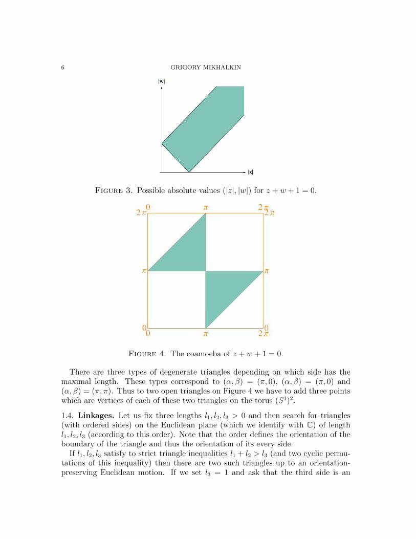
For comparison, Figure 3 depicts the set of pairs of positive real numbers (|z|, |w|)such that |z|, |w| and 1 satisfy to the triangle inequalities. To get Figure 2 fromFigure 3 we just need to reparameterize the picture, namely take the logarithmcoordinatewise.

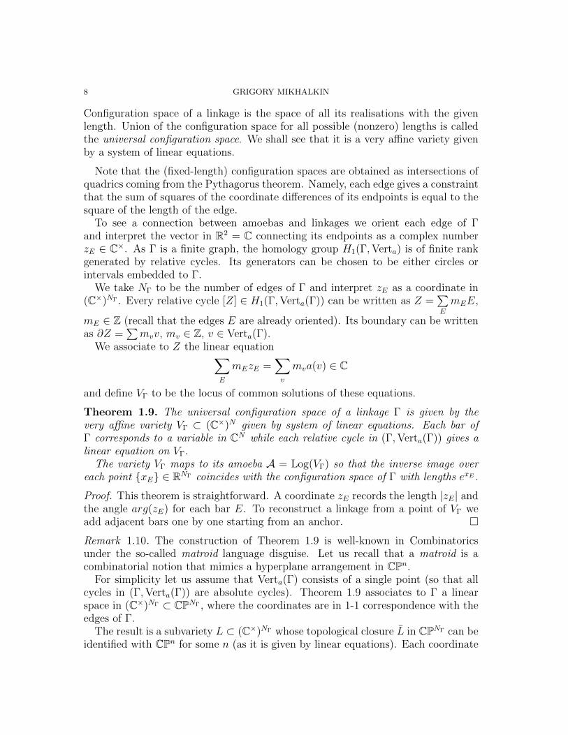
The coamoeba of L is depicted on Figure 4. If 0 < α < π then two of the anglesof the triangle are π−α and π+α−β. All angles of a non-degenerate triangle haveto be between 0 and π, while their sum have to be π. Thus β < α + π and α < β.Similary we get β < α and α < β + π if 0 > α > π.

6 GRIGORY MIKHALKIN

Figure 3. Possible absolute values (|z|, |w|) for z + w + 1 = 0.

Figure 4. The coamoeba of z + w + 1 = 0.

There are three types of degenerate triangles depending on which side has themaximal length. These types correspond to (α, β) = (π, 0), (α, β) = (π, 0) and(α, β) = (π, π). Thus to two open triangles on Figure 4 we have to add three pointswhich are vertices of each of these two triangles on the torus (S1)2.

1.4. Linkages. Let us fix three lengths l1, l2, l3 > 0 and then search for triangles(with ordered sides) on the Euclidean plane (which we identify with C) of lengthl1, l2, l3 (according to this order). Note that the order defines the orientation of theboundary of the triangle and thus the orientation of its every side.

If l1, l2, l3 satisfy to strict triangle inequalities l1 + l2 > l3 (and two cyclic permu-tations of this inequality) then there are two such triangles up to an orientation-preserving Euclidean motion. If we set l3 = 1 and ask that the third side is an


(oriented) interval from −1 to 0 (in C) then there are exactly two such triangles,see Figure 5.

Figure 5. Two triangles in C with given length and of the sides andtwo vertices fixed at −1 and 0.

If l1, l2, l3 does not satisfy to at least one triangle inequality, e.g. l1 + l2 < l3then no such triangles exist. Finally, we may have a non-generic case when one ofthe triangle inequality turns to an equality, e.g. e.g. l1 + l2 = l3. The last casecorresponds to a degenerate triangle (contained in a line). If the third side is fixedas above then we have a unique (degenerate) triangle with these lengths.

Summarising we get the following proposition for the amoeba A = Log(L) of theline L = {z + w + 1 = 0} ⊂ (C×)2. We denote the (topological) interior of A withA◦ and its boundary with ∂A.

Proposition 1.7. If (x, y) ∈ A◦ then Log−1(x, y) ∩ L consists of two points; if(x, y) ∈ ∂A then Log−1(x, y) ∩ L consists of a single point.

Recall that a linkage is a finite graph Γ enhanced with positive lengths associ-ated to its edges and a partition of the set Vert(Γ) of its vertices into two classesVerta(Γ) ∪ Vertm(Γ) of anchored and movable vertices. In addition a (planar) link-age is enhanced with the anchor map a : Verta(Γ) → R2. For technical reasons werequire that Γ is connected and that there is at least one anchor, i.e. Verta 6= ∅.

We interpret this graph as a mechanism with bars (of specified length) correspond-ing to the edges of the graph. The bars are connected at joints which correspondto the vertices of the graph. Anchored vertices are fixed in position determined bythe map a. The bars themselves are rigid, but can be freely rotated at the joints.

Definition 1.8. A realisation of a planar linkage is a map h : Vert(Γ) → R2 withthe following properties.

• We have h|Verta(Γ) = a.• For every edge E ⊂ Γ we have the distance between the images of its end-

points under the map h equal to the length of E.

8 GRIGORY MIKHALKIN

Configuration space of a linkage is the space of all its realisations with the givenlength. Union of the configuration space for all possible (nonzero) lengths is calledthe universal configuration space. We shall see that it is a very affine variety givenby a system of linear equations.

Note that the (fixed-length) configuration spaces are obtained as intersections ofquadrics coming from the Pythagorus theorem. Namely, each edge gives a constraintthat the sum of squares of the coordinate differences of its endpoints is equal to thesquare of the length of the edge.

To see a connection between amoebas and linkages we orient each edge of Γand interpret the vector in R2 = C connecting its endpoints as a complex numberzE ∈ C×. As Γ is a finite graph, the homology group H1(Γ,Verta) is of finite rankgenerated by relative cycles. Its generators can be chosen to be either circles orintervals embedded to Γ.

We take NΓ to be the number of edges of Γ and interpret zE as a coordinate in(C×)NΓ . Every relative cycle [Z] ∈ H1(Γ,Verta(Γ)) can be written as Z =

∑E

mEE,

mE ∈ Z (recall that the edges E are already oriented). Its boundary can be writtenas ∂Z =

∑mvv, mv ∈ Z, v ∈ Verta(Γ).

We associate to Z the linear equation∑E

mEzE =∑v

mva(v) ∈ C

and define VΓ to be the locus of common solutions of these equations.

Theorem 1.9. The universal configuration space of a linkage Γ is given by thevery affine variety VΓ ⊂ (C×)N given by system of linear equations. Each bar ofΓ corresponds to a variable in CN while each relative cycle in (Γ,Verta(Γ)) gives alinear equation on VΓ.

The variety VΓ maps to its amoeba A = Log(VΓ) so that the inverse image overeach point {xE} ∈ RNΓ coincides with the configuration space of Γ with lengths exE .

Proof. This theorem is straightforward. A coordinate zE records the length |zE| andthe angle arg(zE) for each bar E. To reconstruct a linkage from a point of VΓ weadd adjacent bars one by one starting from an anchor. �

Remark 1.10. The construction of Theorem 1.9 is well-known in Combinatoricsunder the so-called matroid language disguise. Let us recall that a matroid is acombinatorial notion that mimics a hyperplane arrangement in CPn.

For simplicity let us assume that Verta(Γ) consists of a single point (so that allcycles in (Γ,Verta(Γ)) are absolute cycles). Theorem 1.9 associates to Γ a linearspace in (C×)NΓ ⊂ CPNΓ , where the coordinates are in 1-1 correspondence with theedges of Γ.

The result is a subvariety L ⊂ (C×)NΓ whose topological closure L in CPNΓ can beidentified with CPn for some n (as it is given by linear equations). Each coordinate


zE in CPNΓ (for an edge E ⊂ Γ) defines a hyperplane zE = 0. Thus all edges of Γdefine a hyperplane arrangement in L.

It is easy to see that the matroid corresponding to this hyperplane arrangementcoincides with the so-called graphics matroid associated to Γ.

Example 1.11. The linkage depicted on Figure 6 has two cycles in the graph Γ, itis the well-known inversor linkage. Its vertex O is anchored at the origin and thetwo bars adjacent to O have the same length equal to R. The other four bars havethe same length equal to r < R.

Moving the bars we may put the vertex A to any point of the annulus centeredat the origin with the outer radius R and the inner radius r. Then the point B(assuming that it is different from the point A as of course there is also a somewhatless interesting realization with A = B) is the result of the inversion of A at thecircle of radius

√R2 − r2 centered at the origin. This means that the points A and

B sit on the same ray emanating from O and |OA||OB| = R2 − r2.

Figure 6. Inversor linkage.

Exercise 1.12. Prove that the linkage from Example 6 indeed performs the inversionas described above.

One of the simplest class of linkages is given by k-polygons when Γk is a cyclicgraph obtained by decomposing a circle into k edges, so that we have only onecycle. The sides of the k-polygon are ordered and oriented as in Figure 7. The onlyanchored vertex is the one where the first and the last edges are joined. We refer toKapovich and Millson [?] for configuration spaces k-polygon linkages.

Given a realisation of the k-polygon linkage we can obtain another one by rotationaround the anchor. To get rid of this obvious symmetry we may fix the last bar ofthe linkage to occupy a given position in R2. Clearly this is the same as anchoringthe second endpoint of the last bar (recall that on its endpoints is already fixed)and removing this bar from Γ, see Figure 8.

10 GRIGORY MIKHALKIN

Figure 7. A k-polygon linkage with k = 5.

Figure 8. The linkage from Figure 7 after deprojectivisation.

By rescaling all lengths lj by the same positive factor we may assume that lk = 1.In this way getting rid of the rotational symmetry of k-polygons amounts to takinga graph Γk homeomorphic to an interval [−1, 0] subdivided into N = k − 1 edgesand anchoring the first endpoint at 0 and the second endpoint at −1. Note thatthe passage to such linkage from a k-polygon linkage corresponds to passing fromprojective to affine coordinates algebraically.

By Theorem 1.9, the universal configuration space of such linkages coincides with

V = {(z1, . . . , zN) ∈ (C)N | 1 +N∑j=1

zj = 0}.

We have considered the case of N = 2 in the previous subsection to determine theamoeba of the line z + w + 1 = 0.

We can use linkages as above, with two anchors and three bars to find the amoebaof the plane 1 + z1 + z2 + z3 = 0. It is easy to see that there are three cases if the


Figure 9. Realizations of a 3 bar linkage with different lengths anddifferent configuration spaces.

lengths 1, l1, l2, l3 are generic. There are no linkage realisation if one of these lengthsis strictly greater than the sum of three others. Otherwise there are two possibilities:when the configuration space consists of a single circle, or of two circles, cf. Figure 9.It is easy to see that the walls separated these possibilities are given by the equation1 + l1 = l2 + l3 and the other two equations corresponding to permutations of lj.

Figure 10. Octahedron.

Exercise 1.13. Take a regular octahedron O (see Figure 10) and colour its faces toblack and white in the chessboard style, i.e. so that no faces of the same colour areadjacent. Let us remove from O the four closed white faces and denote the resultwith A. Show that there exists a homeomorphism between A and the amoeba ofA = A(1 + z1 + z2 + z3 = 0) ⊂ R3 such that ∂A is mapped to the three white facetsand such that the image of the three square diagonals of O separate A r ∂A intoeight regions: four with a single circle over it and four with two circles.

Remark 1.14. Theorem 1.9 provide a linkage interpretation for amoebas of somevarieties given by systems of linear equations. General polynomial equations contain


monomials of arbitrary degree. If we represent each monomial with a bar of Γthere will be some relations, particularly on the slopes of this bar. E.g. the barcorresponding to z2 has to be rotated twice as much as the bar corresponding to z.The rotation of the bar corresponding to zw has to be a combination of rotation ofthe bars corresponding to z and w, etc.

Problem 1.15. Can you invent reasonable mechanisms generalizing linkages sothat they would be capable to describe amoebas of varieties given by non-linearequations?

1.5. Coamoebas of hyperplanes in CPN . To describe the coamoeba B of the

hyperplane determined by 1+N∑j=1

zj = 0 we may use the following simple observation.

Proposition 1.16. We have (0, . . . , 0) 6= (β1, . . . , βN) /∈ B if and only if thereexists a closed arc A ⊂ S1 = R/2π of length π such that {0, β1, . . . , βN} ⊂ A and{0, β1, . . . , βN} 6⊂ ∂A.

In other words, (β1, . . . , βN) ∈ B if they are distributed in the circle R/2πZ (whichwe may view as the unit circle in C with the help of exponentiation) in a non-convexway, see Figure 11.

Figure 11. A collection of points in the unit circle |z| = 1 arrangedin a non-convex way: some positive multiples of these points add upto 0 in C.

Proof. If such an arc A exists then 1 +N∑j=1

rjeiβj must sit in the interior of the half-

space in RN passing through the origin and defined by A for any choice of rj > 0.Otherwise we may choose the weights rj on the unit circle S1 ⊂ C at the pointseiβ1 , . . . , eiβN so that together with the unit weight at 1 they have the center of massat the origin. �

But such collections βj are easy to describe. We may parameterize an arc A oflength π by its most-clockwise endpoint α ∈ S1. Since 0 ∈ A we have −π ≤ α ≤ 0.We can reformulate βj ∈ A as α ≤ βj ≤ α + π.


If α = 0 such conditions on β determine a square 0 ≤ βj ≤ π. For othervalues of α this square has to be translated by α(1, . . . , 1). Thus the closure ofthe complement of B is the Minkowski sum I0 + I1 + . . . IN ⊂ (R/2π)N of theclosed intervals I0, I1,. . . , IN , where I0 = {(−α, . . . , α) | − π ≤ α ≤ 0} andIj = {(0, . . . , 0, βj, 0, . . . , 0) | 0 ≤ βj ≤ π}, j = 1, . . . , N . Recall that Minkowskisum of intervals is called a zonotope.

Note that if {0, β1, . . . , βN} 6⊂ ∂A correspond to the case when eiβj = ±1 for eachβj, i.e. all coordinates zj are real. Thus we have the following proposition.

Theorem 1.17. The coamoeba B1+z1+···+zN=0 ⊂ (S1)N is the union of 2N −1 pointsof the form βj = 0, π with at least one nonzero βj, and the complement of theMinkowski sum I0 + I1 + . . . IN .

Figure 12. The coamoeba of z + w + 1 = 0 in a different frame.

Example 1.18. In Figure 12 we redraw the coamoeba of 1 + z + w choosing thesquare frame for the torus so that the origin is in its center. In this frame we easilysee the hexagon I0 + I1 + I2.

Remark 1.19. Note that in the case N = 2 there is a single point of V1+z+w ⊂ (C×)2

projecting to a point of the coamoeba unless this is one of the three real points(π, 0), (0, π) and (π, π). These three points correspond to the three real quadrantshaving non-empty intersection with V1+z+w. Thus the fiber over each of these specialpoints is an arc.

Exercise 1.20. Visualize topologically V1+z+w fibered over its coamoeba as two disks(from triangles) after gluing three twisted ribbons (from three special points). Showthat topologically it is homeomorphic to a pair-of-pants, i.e. a sphere puncturedat three points. Compare this topological picture with the one coming from theamoeba presentation.


2. Lecture 2: Convexity and behavior at infinity

So far we did not justify the choice of taking the logarithm of the absolute valueof the coordinates in Definition 1.4. Topologically the pictures resulting from takingjust the coordinate absolute value as in Figure 3 or their logarithms as in Figure 2are the same. In this section we start to see advantages of taking the logarithms.

2.1. Convexity of amoebas. The following theorem was one of the motivation fordefining amoebas by Gelfand, Kapranov and Zelevinsky.

Theorem 2.1 ([?]). If V ⊂ (C×)N is a hypersurface then every (topological) con-nected component of RN rA is a convex open domain.

Proof. We already know that the complement of A is open since Log : (C×)N → RN

is a proper map. Convexity of components of RN r A is ensured by the nextlemma. �

Suppose x, x′ ∈ RN . We denote by

[x, x′] = {λx+ (1− λ)x′ | 0 ≤ λ ≤ 1} ⊂ RN

the interval obtained by connecting x to x′.

Lemma 2.2. Let A ⊂ RN be the amoeba of a hypersurface V ⊂ RN . If x, x′ ∈ RN

belong to the same connected component of RN rA then we have [x, x′] ⊂ RN rA.

Proof. Since RN rA is open it is sufficient to prove this lemma for the special casewhen the slope of the interval [x, x′] is rational, i.e. we have c(x− x′) = p ∈ ZN forsome positive real scalar c > 0.

Let us consider a closed geodesic γ in the phase torus (S1)N = (R/2π/Z)N realis-ing the homology class p ∈ ZN = H1(R/2πZ)N . All such geodesic foliate the torusγ and are parameterised by the (N − 1)-dimensional quotient torus (S1)N/γ.

The key observation for this lemma is that

[x, x′]× γ ⊂ RN × (S1)N = (C×)N

is a holomorphic annulus. Indeed, we have log |zj| = Re(log(zj)) while arg |zj| =Im(log(zj)). Thus the multiplication by i takes a vector tangent to RN × {β} tothe corresponding vector tangent to {x} × (S1)N . The correspondence for tangentvectors here is given by the tautological identifying the tangent vectors to (S1)N =(R/2πZ)N with RN .

Suppose that [x, x′] ∩ A 6= ∅. Then we have

([x, x′]× γ) ∩ V 6= ∅

for one of the closed geodesics γ in the phase torus (S1)N = (R/2πZ)N realizing thehomology class p ∈ ZN = H1(R/2πZ)N (as such geodesics foliate the whole phasetorus).


Varieties V and [x, x′]× γ are holomorphic varieties of complimentary dimension.The boundary ∂([x, x′] × γ) = {x, x′} × γ is disjoint from V . Thus the topologicalintersection number V and [x, x′]× γ is a well-defined positive number.

But if x and x′ belong to the same component of RN rA then there exists a pathδ ⊂ RN rA connecting x with x′. Clearly, δ × γ ∩ V = ∅, thus ([x, x′] ∪ δ)× γ hasa positive intersection number with V . But [x, x′] ∪ δ is a closed path in RN andthus is null-homologous. Therefore, ([x, x′] ∪ δ) × γ is null-homologous as well andits intersection number with any homology class with closed coefficients in (C×)N

(such as V ) must be zero. We get a contradiction. �

Remark 2.3. As it was noticed by Kapranov, the convexity of amoebas can be viewedas a generalisation of Hadamard’s three-circle theorem. Let us recall its classicalformulation (with three circles).

Given three concentric circle in the complex plane of radii R1 < R2 < R3 around0 and a holomorphic function f in a neighbourhood of the closed annulus R1 ≤ |z| ≤R3 we have

log( max|z|=R2

|f(z)|) ≤ log(R3)− log(R2)

log(R3)− log(R1)log( max

|z|=R1

|f(z)|)+log(R2)− log(R1)

log(R3)− log(R1)log( max

|z|=R3

|f(z)|).

This theorem has another classical reformulation: the function

M(x) = max|z|=ex

log |f(z)|

is convex on an open interval I ⊂ R for any holomorphic function defined in adomain U ⊃ log−1(I).

But, clearly, M(x) is nothing but the upper boundary of the amoeba of the curvew = f(z) (defined in the strip I × R). Such convexity is assured by Theorem 2.1(which clearly works equally well for amoebas defined not only in RN , but also inany contractible domain in RN).

Example 2.4. Let us consider a polynomial function f(z) =∑j=0

ajzj where all

coefficients aj > 0 are positive. We note that the logarithmic image

C = {(x, y) ∈ R2 | ey = f(ex)},

of the graph of the function w = f(z) restricted to the positive value of z is acomponent of the boundary of the amoeba A of

V = {(z, w) ∈ (C×)2 | w = f(z).

Indeed, we have f(ex+iα) ≤ f(ex) by the triangle inequality. Therefore, C ⊂ ∂A,namely C is the upper boundary of A in R2.

The curve C is also the boundary of the closed domain

D = {(x, y) ∈ R2 | ey ≥ f(ex)},


which is a connected component of R2rA and therefore must be convex by Theorem2.1.

We deduce the following (classical) logarithmic convexity property for polynomialsf in one variable with positive coefficients.

(2.1) f(eu+v

2 ) ≤√f(eu)f(ev).

Similar convexity holds also for polynomials in several variables with positive coeffi-cients. (Deduction of this property from convexity of amoebas is due to Kapranov.)

Local positivity of intersection of complex varieties of complimentary dimensionin CN is one of the manifestation of the maximum principle. We may also de-duce convexity of amoebas directly from the maximum principle as each coordinatelog |zj| = Re log(zj) or their linear combination restricted to V is a real part of aholomorphic function and thus a pluriharmonic function.

The following statement holds without assuming that V is a hypersurface andis a variation of Theorem 2.1 Let us however keep the assumption that V is irre-ducible. Let H be a (closed) half-space in RN whose boundary ∂H ⊂ RN is an affinehyperplane.

Theorem 2.5. Suppose that ∂H is a locally supporting hyperplane for A at x, i.e.there exists an open convex domain U ⊂ RN such that A ∩ U ⊂ H then A ⊂ ∂H.

Proof. The half-space H is given by a vector u = (u1, . . . , uN) ∈ RN and a numbera ∈ R through the inequality u.x ≤ a. The linear combination

N∑j=1

uj log |zj|

is a harmonic function on V and by assumption a is its local maximum. By themaximum principle this means that the function is constant so that A ⊂ ∂H. �

Suppose now that dimV = n, so that its codimension is k = N − n. We mayrefine Theorem 2.5 once k is known.

Let L ⊂ RN be a k-dimensional affine space and S ⊂ L is a closed ((k − 1)-dimensional) hypersurface in L. As L is contractible the hypersurface S can bepresented as the boundary S = ∂D for a closed domain D ⊂ L.

Theorem 2.6 (cf. [?],[?]). If L ∩ A = ∅ and [S] is trivial in Hk−1(RN r A) thenD ∩ A = ∅.

Proof. We proceed as in the proof of Theorem 2.1. First we note that we mayperturb the affine space L to ensure that it has rational slope, i.e. there exist klinearly independent integer vectors tangent to L. Since A is closed for a sufficientlysmall perturbation a hypersurface S disjoint from A will be retained.

Thus we may assume that the slope of L ⊂ RN is rational and thus its quotientin L ⊂ RN/(2πZN) is a closed k-dimensional subtorus of (S1)N . All k-subtori γ


parallel to it foliate (S1)N with the quotient homeomorphic to (S1)N−k. Note thatL× γ is a k-dimensional complex subvariety for any γ from this foliation.

Suppose that D∩A 6= ∅. Then D×γ ∩V 6= ∅ for a k-subtorus γ in this foliation.As ∂D × γ is disjoint from V the intersection number of D × γ and V is well-defined and must be positive as intersection number of two complex subvarieties ofcomplementary dimension.

But if S = ∂D bounds a k-cycle δ in the complement of A the closed cycle(D∪δ)×γ has the same positive intersection with V as D×γ. We get a contradictionas D ∪ δ is a trivial k-cycle in L (as any other positive-dimensional cycle in acontractible space). �

Remark 2.7. Theorem 2.6 says that it is not possible to find a k-plane L that cutsA inside a domain D ⊂ L so that ∂D is disjoint from A and homologically trivial inRN rA. In classical geometry such a domain is sometimes called a cutting k-cap, soTheorem 2.6 says that it is not possible to cut a k-cap from the amoeba of a varietyof codimension k.

The condition that ∂D is homologically trivial in RN r A is necessary as it canbe seen already for amoebas of spatial curves, cf. the next example.

Example 2.8. Let V ⊂ (C×)3 be the twisted rational cubic curve given by theparameterisation

t 7→ (t, t− 1, t− 2), t ∈ C× r {1, 2},

see Figure ??. Since the parametrisation is defined over R, the conjugate points ofC× r {1, 2} are mapped to the same point of the amoeba of V .

Thus the amoeba A is the image of the quotient of C× r {1, 2} under the invo-lution of complex conjugation, which is topologically the disk minus four points atits boundary. It is easy to see that near three of these punctures (namely, 0, 1, 2)the amoeba A has asymptotes in the three coordinate directions. It goes to (−∞)-direction as the corresponding coordinate before taking the logarithm vanishes. Nearthe fourth puncture (which corresponds to∞) the amoeba A has a diagonal asymp-tote, it is parallel to the vector (1, 1, 1).

Let us consider the intersection ofA by the plane L = {(x1, x2, x3) ∈ R3 | x1+x2 =0}. The intersection points correspond to solutions of log |t| + log |t − 1| = 0 or|t(t− 1)| = 1. It is easy to see that a circle of sufficiently large radius in L centeredat the origin (0, 0, 0) is disjoint from A. In the same time the disk bounded by thiscircle intersect A. This circle is not nomologically trivial in H1(R3 rA) as e.g. itslinking number with the path connecting the punctures 0 and ∞ is non-zero.

In the same time, in accordance with Theorem 2.5 the amoeba A ⊂ R3 is hyper-bolically embedded to R3: its Gaussian curvature is nowhere positive.

2.2. Behavior of amoebas at infinity. As we have seen, the amoeba A is closed.But it can never be compact for positive-dimensional very affine varieties V as such


varieties themselves are non-compact while Log |V is proper. ThusA has to approachinfinity at RN .

One way to see a neighborhood of infinity at (C×)N is to compactly it to CPN andthen look at the neighborhood of ∂CPN = CPNr(C×)N . By the very construction ofthe projective space the boundary ∂CPN consists of N + 1 coordinate hyperplanes:N corresponding to the coordinate zeroes zj = 0 which we have to put back torecover CN from (C×)N . The remaining hyperplane in ∂CPN corresponds to theinfinite plane CPN rCN in projective geometry. It can also be seen as a coordinateplane once we change the coordinates in (C×)N according to another coordinatechart in CPN , e.g. in coordinates z−1

1 , z2z−11 , . . . , zNz

−11 . These coordinate charts

can be identified with each other with the help of a natural multiplicative-linearaction of GL(N,Z) on (C×)N .

Namely, for a matrix m = (mjk) ∈ GL(N,Z) we define

(2.2) m(z1, . . . , zN) = (N∏j=1

zm1j

j , . . . ,N∏j=1

zmNj

j ).

Proposition 2.9. The action (2.2) of GL(N,Z) on (C×)N is consistent with itstautological action on RN . Namely, the diagram

(C×)N //

Log��

(C×)N

Log��

RN // RN

,

where the horizontal arrows correspond to the actions my any element m ∈ GL(N,Z),is commutative.

Proof. The proposition is a straightforward corollary of the logarithm propertylog |zw| = log |z|+ log |w|. �

Thus any primitive integer vector v ∈ ZN can be thought of as a coordinatedirection (0, . . . , 1) in RN after a suitable GL(N,Z) coordinate change.

Let us consider the slices

At = A ∩ {xN = t}of A by the horizontal hyperplanes in RN . Forgetting the coordinate xN we mayinterpret At as a subset of RN−1 depending on the parameter t ∈ R.

Let us consider the topological closure V in (C×)N−1 ×C of V ⊂ (C×)N . Denote

V−∞ = V ∩ (C×)N−1 × {0} = (C×)N−1.

We may consider the amoeba A−∞ of V−∞ as a subset in RN−1.

Proposition 2.10 (cf. [?]). We have

A−∞ = limt→−∞

At.


Furthermore, we may describe A−∞ as the set of points (x1, . . . , xN−1) ∈ RN−1 suchthat for any neighborhood U ⊂ RN−1, U 3 (x1, . . . , xN−1) and M ∈ R, we have

U × (−∞,M ] 6= ∅.In particular, A−∞ is a well-defined set in the quotient of RN by the (0, . . . , 0,−1)-direction and is invariant under a coordinate change in (C×)N as long as the direc-tion (0, . . . , 0,−1) is constant in the first N − 1 new coordinates and decreases thevalue of the last coordinate.

Similarly, we may describe V−∞ as the set of points (z1, . . . , zN−1) ∈ (C×)N−1

such that for any neighborhood U ⊂ (C×)N−1, U 3 (z1, . . . , xN−1) and M ∈ R, wehave

U × {0 < |zN | < eM} 6= ∅.It is also invariant with respect to coordinate changes described above.

The limit here is taken in the sense of Hausdorff metric on compact sets in RN .This means that for every compact set K ⊂ RN we have

limt→−∞

d(K ∩ At,A−∞) = 0,

where d stands for the Hausdorff distance between the sets, i.e. the maximumpossible distance between one set and a point of the other.

Proof. The proposition follows from the similar statement about the limit of V ∩{zN = et+αi} ⊂ (C×)N−1. The limit of these sets when t → −∞ is V ∩ {zN = 0}since V is algebraic and is obtained as the topological closure of V . �

For any vector v ∈ RN we may define the affine space RN/v ≈ RN−1 as thequotient space of RN by all lines parallel to v. Similarly, we define (C×)N/v ≈(C×)N−1 as the quotient space of (C×)N by C×-subtori parallel to v, so that Logprovides a well-defined map from (C×)N/v to RN/v. We may define the v-infinitedirection amoeba as

(2.3) A∞v = {x ∈ RN | {U + (M + t)v | t > 0} 6= ∅ ∀U 3 x, ∀M ∈ R}/v ⊂ RN/v.

Here U is any open neighborhood of x in RN .Clearly, A∞(0,...,0,−1) = A−∞ from Proposition 2.10. We define the variety V ∞v

as V−∞ under a suitable coordinate change from Proposition 2.9. We call it thev-infinite variety for V ⊂ (C×)N .

Definition 2.11. We say that v ∈ RN is a A-limiting direction if A∞v 6= ∅. Theunion Log of all limiting directions and {0} is called the limiting set, or the Bergmanfan (see Theorem 2.13) of V ⊂ (C×)N .

Definition 2.12. A set C ⊂ RN is called a polyhedral cone if it is the intersectionof finitely many closed half-spaces Hj passing through the origin 0 ∈ RN . EachHj is defined by the inequality uj.x ≥ 0 for the scalar product uj.x with a vector


uj ∈ RN . A polyhedral cone C is called Z-polyhedral if uj ∈ ZN for all j. A face ofC is cut on C by a system of equations uj.x = 0 for some j.

A Z-polyhedral fan F is a collection of Z-polyhedral cones such that

• whenever a cone C is contained in F all of its faces are also contained in F ,• the intersection of any subcollection of cones in F is the common face of all

cones in the subcollection.

We say that F is n-dimensional if it is a finite union of n-dimensional Z-polyhedralcones and their faces. We often identify the fan F (as a collection of cones) withthe set

F =⋃C∈F

C ⊂ RN

which we also call a fan.

Recall that the basic construction of toric geometry (see e.g. [?], [?]) provides apartial compactification TF of (C×)N for a Z-polyhedral fan F . Each cone C ∈ Fcorresponds to stratum TC ⊂ TF .

Theorem 2.13 (cf. Bergman [?]). Let V ⊂ (C×)N be a n-dimensional algebraic va-riety. The limiting set L ⊂ RN of all A-limiting direction is a (finite) n-dimensionalZ-polyhedral fan.

Furthermore, the topological closure V of V in TF is compact and the variety V istransversal to the stratum TC for each cone C ∈ L. If a vector v ∈ RN belongs to therelative interior of C then V ∞v ⊂ (C×)N/v is invariant with respect to multiplicationby any vector parallel to C. The quotient of V ∞v by the subtorus formed by suchvectors coincides with V ∩ TC (note that TC is the quotient of the whole (C×)N bythis subtorus).

We postpone the proof of this theorem until later in these lectures. We’ll also seethat the Z-polyhedral fan L in this theorem satisfies to a certain balancing condition(which is a fundamental property in tropical geometry).

Remark 2.14. We may rephrase the last part of Theorem 2.13 without use of toricgeometry language as follows. If v ∈ RN belongs to the relative interior of a k-dimensional cone C ∈ F then V ∞v ⊂ (C×)N/v is invariant with respect to multipli-cation by any vector parallel to C/v. If v′ ∈ C ′, where C ′ is a face of C, then we mayconsider the v-infinite variety V ∞,∞v′,v ⊂ ((C×)N/v)/v′ for V ∞v′ (taking the quotient of

v in RN/v′). This variety coincides with the quotient of V ∞v in ((C×)N/v)/v′.

2.3. Behavior of coamoebas at infinity. The map Arg |V : V → (S1)N is notproper, but its target is compact. Thus the limit of the ends of V should give us apotentially interesting subset in (S1)N .


Namely, let us consider an exhausting family of compact sets Kj ⊂ V , Kj ⊂ Kj+1,

j ∈ {1, . . . , n},N⋃j=1

Kj = V and the topological closures Arg(V rKj) in (S1)N of

the images of their complements.

Definition 2.15 (also called the phase-limit set, see [?]). We define the infinitylocus of coamoeba as

B∞ =∞⋂j=1

Arg(V rKj) ⊂ (S1)N .

It is convenient to consider the topological closure B of B in (S1)N . We call it theclosed coamoeba of V .

As the restriction of the map Arg to a compact set Kj is proper for any j, we getthe following proposition.

Proposition 2.16. The set B r B∞ is closed in (S1)N r B∞. In other words,

∂B r B ⊂ B∞.

Corollary 2.17.

B = B ∪ B∞.

The corollary follows from Proposition 2.16 since B∞ ⊂ B by the definition ofB∞.

The complement of Kj in V for large j can be thought of as a neighbourhood of

V ∞ = V r V

in the compactification V (defined in Theorem 2.13) after removing the set V ∞ itselffrom this neighborhood. For each cone C ∈ L we consider a family of open sets

UCj ⊂ V , UC

j ⊃ UCj+1, j ∈ {1, . . . , n}, such that

∞⋂j=1

UCj = C. We define

B∞C =∞⋂j=1

Arg(UCj ) ⊂ (S1)N .

As in the previous subsection we may consider the linear projection

πC : (C×)N → (C×)N/C

obtained by taking the quotient of (C×)N by the subtorus parallel to C. (Clearly,(C×)N/C ≈ (S1)N−k, where k is the dimension of C.) Furthermore, we may considerthe coamoeba BC ⊂ (C×)N/C of V ∞C .

Proposition 2.18. We have

B∞C = π−1C (BC).


This proposition follows from Proposition 2.10. As a neighborhood of V ∞ de-composes into the union of neighborhoods of its strata V ∞C we get the followingstatement.

Corollary 2.19 (cf. [?], [?]). The infinity locus of B is a closed set in (S1)N thatcan be decomposed in the following way:

B∞ =⋃C

π−1C (BC).

Example 2.20. We see the three geodesics on the torus that form B∞ in the caseof the line {z + w + 1 = 0} depicted on Figure 4.

2.4. Convexity of coamebas. Outside of its infinity locus B∞ the coamoeba pos-sesses the same convexity properties as the amoeba. In fact, its proof is even easieras the fiber of the map Arg is contractible.

As usual, we start from the case when V is a hypersurface.

Theorem 2.21 (cf. [?]). For every connected component U of (S1)N r B∞ the setUrB is convex. This means that if I ⊂ U is a geodesic interval such that ∂I∩B = ∅then I ∩ B = ∅.

Proof. Let I ⊂ (S1)N be such an interval and L ⊂ RN be a line parallel to I (asusual, we identify RN with the universal covering space of (S1)N). There is a (N−1)-dimensional family of such lines parameterized by RN/I ≈ RN−1 that provides afoliation of RN . For any leaf L of this foliation the product

L× I ⊂ RN × (S1)N = (C×)N

is a holomorphic annulus.Since I is disjoint from B∞, the set Arg−1(I) ∩ V is compact. Therefore, (L ×

I)∩V = ∅ if L is sufficiently close to infinity in RN/I, but it is non-empty for someleaves L if I ∩B 6= ∅. We get a contradiction to positivity of intersection of complexsubvarieties of complimentary dimensions in (C×)N . �

Now we treat the general case when dimV = N − k. Suppose that K ⊂ RN isa k-dimensional linear space, S ⊂ K is a closed hypersurface and D is the closeddomain in K bounded by S. We denote by S and D the images of S and D inRN/2πZN ≈ (S1)N .

Theorem 2.22. If D ∩ B∞ = ∅ and S ∩ B = ∅ then D ∩ B = ∅.

In other words, there is no cutting k-cap for the coamoeba of a variety of codi-mension k in (C×)N . Note that unlike the case with Theorem 2.6 we do not requireany homological triviality for S.

Proof. We consider all k-dimensional linear spaces L that are parallel to K. AsArg−1(D) ∩ V is compact we have L×D ∩ V = ∅ if L is close to infinity in RN . In


the same time there exists a choice of L with L ×D ∩ V 6= ∅ (and thus a positiveintersection number) if D ∩ B∞ 6= ∅. �

grigory mikhalkin - sciencesmaths-paris.fr et resumes cours... · 2 grigory mikhalkin 1. lecture 1:...

Documents