greedy block coordinate descent (gbcd) method for … block coordinate descent (gbcd) method for...

Greedy Block Coordinate Descent (GBCD) Methodfor High Dimensional Quadratic Programs

Gugan ThoppeSchool of Technology and Computer Sc., Tata Institute of Fundamental Research, Mumbai 400005, India, [email protected]

Vivek S. BorkarDepartment of Electrical Engineering, Indian Institute of Technology Bombay, Mumbai 400076, India, [email protected]

Dinesh GargIBM Research - India, Manyata Embassy Business Park, Bangalore 560045, India, [email protected]

High dimensional unconstrained quadratic programs (UQPs) involving massive datasets are now common

in application areas such as web, social networks, etc. Unless computational resources that match up to

these datasets are available, solving such problems using classical UQP methods is very difficult. This paper

discusses alternatives. We first define high dimensional compliant (HDC) methods for UQPs—methods that

can solve high dimensional UQPs by adapting to available computational resources. We then show that the

class of block Kaczmarz and block coordinate descent (BCD) are the only existing methods that can be

made HDC. As a possible answer to the question of the ‘best’ amongst BCD methods for UQP, we propose

a novel greedy BCD (GBCD) method with serial, parallel and distributed variants. Convergence rates and

numerical tests confirm that the GBCD is indeed an effective method to solve high dimensional UQPs. In

fact, it sometimes beats even the conjugate gradient.

Key words : quadratic optimization; high dimensions; greedy block coordinate descent

1. Introduction

Machine learning and statistics problems arising in application areas such as the web, social net-

works, e-commerce, m-commerce, etc. are often extremely large in size. As described in Boyd et al.

(2011), these problems typically share two characteristics—(1) the input datasets are staggeringly

large, consisting of millions or billions of training examples, and (2) the data describing each exam-

ple is itself high-dimensional. While many of these problems are still convex optimization programs,

the above two high dimensional characteristics bring in new challenges concerning management of

data. The worst is when the available computational setup to solve these problems is itself minimal

and simplistic. As a result, methods which can solve large scale optimization problems by adapting

to the resources available are now of central importance. We will refer to such methods as high

dimensional compliant (HDC) methods. In this paper, we aim to build HDC solution methods for

an unconstrained quadratic program (UQP)—the simplest convex optimization problem.

Recent literature, see Nesterov (2012), Richtarik and Takac (2012), Needell and Tropp (2014),

etc., suggests that block Kaczmarz (BK) and block coordinate descent (BCD) class of methods

1

arX

iv:1

404.

6635

v3 [

mat

h.O

C]

12

Jul 2

014

2 Thoppe, Borkar and Garg: Quadratic Optimization in High Dimensions

may be the only ones suited to tackle large scale optimization. A rigorous verification of this belief

has, however, been missing. In this paper, we first define the notion of HDC solution methods for

UQP. We then show that BK and BCD are the only existing UQP solution methods which can be

made HDC. In fact, we prove that even natural generalizations of the BK and BCD philosophies

are not HDC. This then brings us to the question of which is the ‘best’ amongst BK and the

‘best’ amongst BCD methods for a UQP. As a possible answer to the latter, we propose a novel

deterministic, but adaptive, greedy BCD (GBCD) method with serial, parallel, and distributed

variants. Convergence rates and numerical tests confirm that GBCD is indeed an effective method

to solve high dimensional UQPs. In fact, it sometimes beats even the conjugate gradient.

1.1. Preliminaries

Throughout this paper, a UQP will essentially be assumed to have the general form

minx∈Rn

f(x) =1

2xtPx−xtq+ r, (1)

where P ∈ Sn++ ⊂Rn×n, i.e., the matrix P is symmetric and positive definite, q ∈Rn and r ∈R. We

will often refer to P as the input matrix. Since the gradient of the quadratic function f is

∇f(x) = Px− q (2)

and P ∈ Sn++, it is easy to see that solving (1) is equivalent to solving the linear system of equations

Px= q. (3)

Thus the unique optimal point to (1) is

xopt = P−1q (4)

and the optimal value is

f(xopt) = r− 1

2qtP−1q. (5)

The matrix P induces the norm

||x||P :=√xtPx. (6)

In view of (1), (5), and (6), we have

f(x)− f(xopt) =1

2||x−xopt||2P . (7)

A method that uses knowledge of P, q and r and obtains accurate estimates of (4) and/or (5) is

called a solution method for (1).

We will say that the UQP in (1) is high dimensional, i.e., it shares the aforementioned high

dimensional characteristics, if n is high, say of the order of 105 or more, and the matrix P is dense,

i.e., almost all its entries are nonzero. In what follows, we spell out the challenges involved in

solving a high dimensional version of (1) when only limited computational resources are available.

Thoppe, Borkar and Garg: Quadratic Optimization in High Dimensions 3

1.2. Computational Challenges for a High Dimensional UQP

• There is a limit on the size of main memory and secondary storage: Under present

hardware technology, main memory (i.e., RAM) size of a processor is of the order of a few Giga-

Bytes (GB) while secondary storage devices go up to few TeraBytes (TB). But observe, as an

example, that when n= 220 ≈ 106, the minimum space required just to store the n2 entries of P is

8 TeraBytes—assuming double precision, i.e., 8 Bytes per entry. This implies that to tackle a high

dimensional UQP, we firstly need several secondary storage devices to store P. Second, it becomes

a necessity to slice the large P into numerous chunks and store them in a distributed manner across

multiple secondary storage devices. Third, only a few chunks, i.e., a small portion of the large P,

can be loaded into the main memory of a single processor at any given time.

• Computing f(x) or ∇f(x) has long running time: With the above memory issues, reading

a large P matrix into the main memory of a single processor, if there is such a need, can be done

only in a chunk by chunk manner. This implies that, with a single processor, even the simple matrix

vector multiplication Px will have to be done only in a piecemeal fashion in high dimensions.

Although the time complexity of this operation still remains O(n2), multiple secondary storage

accesses, especially from noncontiguous locations, will add a nontrivial overhead.

But observe from (1) and (2) that computing f(x) or ∇f(x) at any arbitrary point x ∈ Rn

necessarily involves the operation Px. Consequently, in high dimensions, any method that uses

function values and/or gradient values to iteratively improve the solution quality will have to suffer

an extremely large running time per iteration on a single processor; several hours per iteration is

not unimaginable for n just a million in size.

• Parallelization offers little help: The running time of the operation Px discussed above

can definitely be cut down by parallelizing the computation across multiple processors. However,

due to budgetary constraints, practitioners usually have access to only a fixed finite number of

processors at any given time. These limited resources imply that, in high dimensions, the per

iteration running time of methods that use function/gradient values to iteratively improve the

solution quality can be cut down only marginally, usually only by a constant factor.

We would like to mention here that if (1) can be decomposed into a small number of independent

problems then each of these problems can be accommodated and solved in parallel on independent

machines. This idea is applicable whenever the matrix P has an inherent block diagonal structure

with small number of blocks. But our interest lies in high dimensional setups where the matrix P

is dense. As pointed out by Richtarik and Takac (2012), the only way here may be to appeal to a

serial method leveraging a single processor or a fixed number of processors.

Circumventing the above challenges is the aim here. That is, we presume the availability of only

a simplistic computational setup throughout the paper. This setup, referred to henceforth as the

finite main memory (FMM) setup, is assumed to have:


1. a single processor with limited main memory and

2. finite sized secondary storage devices in numbers large enough to store the input data of the

high dimensional UQP that is to be solved.

Our goal then is to develop methods that can solve (1) even when n is so large that the size of

P far exceeds the limited main memory size in the available FMM setup. Note that in theoretical

analysis of a serial method having a single processor or finite number of processors makes no

difference. For this reason and for pedagogical convenience, the FMM setup is assumed to have

only a single processor. While discussing parallel and distributed implementation of the proposed

GBCD method in Section 7, we will use setups with multiple processors.

1.3. Desiderata for a High Dimensional UQP Method

We describe here a set of features that practitioners would prefer in an ideal solution method for

a high dimensional version of (1) given only the FMM setup.

FFF1. Work with only subset of entries of P at one time. The reason being that when n

is very large, the available main memory in FMM setup will be orders of magnitude smaller than

the total data size of the matrix P.

FFF2. Possess low per iteration running time (subquadratic in n). In view of the discussion

in the previous subsection, this feature essentially says that the method should never compute

either f(x) or ∇f(x) explicitly for any x during the entire course of its execution.

FFF3. Use hard partitioning of P . That is, the method should suggest an explicit partition of P

into chunks that can be stored across multiple hard disks. After the partitioning, no major shuffling

of the data should be required. This is needed because moving data within/across secondary hard

disks is an extremely time consuming process. Furthermore, at any given time, the method should

require to load data only from one or a few select chunks of P into the main memory . The reason

being that disk access time for non-contiguous data, as against contiguous data stored in the form

of a chunk, is extremely high.

From now on, we will say that a solution method for (1) is high dimension compliant

(HDC) if and only if it has all the three features mentioned above. In addition to these basic

features, one would optionally prefer that the HDC method has following desirable features as well.

FFF4. Possess comparable running time. That is, the total running time (iteration run time

× number of iterations) of the method to find an approximate solution to xopt should be no worse

than the best of the existing methods.

FFF5. Give scope for parallel and distributed implementation. That is, given a parallel

and/or distributed computing environment, the method should be able to take advantage and

achieve a speedup in its execution time by some factor.


1.4. Contributions and Outline

In Section 2, we survey popular UQP solution methods and show that BK and BCD are the only

existing methods that can be made HDC. In section 3, we prove that even natural generalizations

of BK and BCD are not HDC. To the best of our knowledge, we are the first ones to prove such

results. These results will show that coming up with better BK and BCD methods is indeed the

right way forward for developing solution methods for high dimensional UQPs. In line with this

view, we propose the GBCD method in Section 4. We also discuss results here which show that the

equivalent greedy BK method is non-HDC. We establish bounds on the convergence rate of GBCD

method in Section 5 and discuss heuristic ways to improve it in Section 6. Parallel and distributed

implementations of GBCD are discussed in Section 7. Simulation results comparing GBCD with

popular UQP solution methods are given in Section 8. We finally conclude in Section 9.

2. Survey of Existing UQP Methods and Research Gaps

We survey here the important UQP solution methods by grouping them into three categories—

direct methods, classical iterative methods, and HDC methods. To solve a UQP, broadly speaking,

the members of the first two categories essentially require that the input matrix be entirely available

in the main memory. Consequently, these methods, unless modified, are inappropriate for solving

high dimensional UQPs in an FMM setup. The third category includes the BK and BCD class of

methods. As will be seen, these are the only existing methods that can be easily made HDC. After

this survey, we discuss research gaps in state-of-the-art literature on BK and BCD methods.

2.1. Direct Methods

To solve the UQP in (1), direct methods, see Bertsekas and Tsitsiklis (1989), Davis (2006), begin by

factorizing P using techniques such as SVD, Cholesky decomposition, etc. The factored form of P is

then used to find (4) and (5) in finite steps. These methods take O(n3) time, especially if P is dense,

before giving out the final solution. Popular members in this category include Gaussian elimination,

Cholesky factorization, etc. When n is really small, say less than 103, direct methods are highly

preferred. However, the lack of intermediate solutions coupled with the enormous difficulty in

factorizing a matrix, when it is stored in a distributed fashion, makes direct methods unfavourable

for solving high dimensional UQPs in the FMM setup. These methods are clearly non-HDC.

2.2. Classical Iterative Methods

These methods solve a UQP by using its function/gradient values repeatedly to generate a sequence

of improving solution estimates of (4) and/or (5). These are strongly favored when n is moderately

large, say roughly from 103 upto 105. However, the O(n2) running time per iteration for these


methods makes them non-HDC. Specifically, these methods tend to have exorbitant waiting times

before each update of the solution estimate when used to solve a high dimensional UQP. If, however,

this is not an issue, then, after appropriate modifications, one can go ahead and use these methods

to solve high dimensional UQPs even in the FMM setup.

Classical iterative methods for UQPs can be broadly subdivided into line search methods, cutting

plane methods, and direct search methods. A line search method, see Wright and Nocedal (1999),

uses the following idea in every iteration. It first decides upon a search direction. Along this direction

starting from the current estimate, the point that is closest to the optimal point of the given UQP,

i.e., xopt, under appropriate norm, is then declared the new estimate. Important algorithms here

include the steepest descent and the conjugate gradient. Both these methods use the gradient, after

suitable modifications, to generate the search direction in each iteration. The || · ||P norm from (6)

is used to decide the new estimate in each iteration.

Another category of UQP methods that use gradients are the cutting plane methods, see Kelley

(1960), Levin (1965). Here, the idea is to start with a feasible set containing xopt. Using a hyperplane

normal to the gradient at its centre of gravity, the feasible set is cut into two parts. The side

containing xopt is then called the new feasible set and the above idea is repeated. A major difficulty

here is the efficient computation of the centre of gravity of the feasible set. This can itself turn

out into a very hard problem if the feasible region is arbitrary. Alternatives such as the ellipsoid

method, see Bland et al. (1981), etc., have been proposed to overcome this issue. However, these

alternatives need suitable revisions before they can be used to solve a high dimensional UQP in

the FMM setup.

Direct search methods, see Kolda et al. (2003), avoid gradients and use only function values

to sequentially improve the solution quality. The Nelder and Mead (1965) simplex algorithm is a

key member here. To solve a UQP, this method begins with a n−dimensional simplex. Using a

sequence of reflection, expansion, contraction, and reduction type transformations on the simplex,

the method sequentially reduces the function values at each of its vertices. The Nelder-Mead

approach is, however, known to be slower in convergence in comparison to gradient based schemes

described above. Hence this simplex based approach should not be used to solve a high dimensional

UQP in the FMM setup even if O(n2) running time per iteration is not an issue.

2.3. HDC Methods

We include in this category exclusively the class of BK and BCD methods. These are also iterative

methods that follow the line search principle. However, relative to classical line search methods

mentioned before, the BK and BCD methods use a very different approach to solve a UQP. First,

the BK and BCD methods never explicitly compute function/gradient values. Second, in each


iteration, they need only finite rows of the input matrix. As we shall see at the end of this subsection,

these are also the reasons why BK and BCD methods can be made HDC.

2.3.1. Block Kaczmarz (BK) Methods: The fundamental member of this class is the

simple Kaczmarz (1937) method. To solve the UQP in (1), this method uses precisely one row of

the input matrix P in every iteration. Its update rule is given by

xk+1 = xk +P ti (PiP

ti )−1 (qi−Pixk), (8)

where Pi is the ith row of matrix P. The index i is chosen in a round robin fashion from one

iteration to another.

Elfving (1980) generalized the above idea. We will refer to his method as the traditional BK. As

opposed to (8), the traditional BK method uses multiple rows of P per iteration. More formally,

the traditional BK method first partitions the rows of P into different blocks. Suppose that the

row submatrices Pπ1 , . . . , Pπm denote these blocks, where Π≡ {π1, . . . , πm} represents a partition of

the row index set [n] := {1, . . . , n}. The traditional BK method then uses these blocks in a round

robin fashion across iterations for improving the solution estimate. In notations, its update rule is

xk+1 = xk +P tπi

(PπiPtπi

)−1 (qπi −Pπixk), (9)

where qπi is the subvector of q corresponding to the row indices given in πi.

Clearly, there are two ways in which the traditional BK method can be modified.

1. Input partition Π: Which partition of the rows of P to use at the beginning of the method?

2. Block Selection Strategy ζb: Which block to work with in each iteration of the method?

By choosing appropriately these strategies, one can obtain different BK methods. The BK

method in generic form is given in Algorithm 1. We emphasize here that the convergence rate of a

BK method strongly depends on the choice for both Π and ζb.

Algorithm 1 Generic Block Kaczmarz (BK) Method

Input: initial guess x0 ∈Rn, partition Π≡ {π1, . . . , πm} and strategy ζb

Main Procedure:

for k= 0,1, . . . , do

Using strategy ζb, pick a block Pπi from the available set of blocks.

xk+1← xk +P tπi

(PπiPtπi

)−1(qπi −Pπixk).

end for


2.3.2. Block Coordinate Descent (BCD) Methods: The counterpart of the simple Kacz-

marz method in the BCD class is the Gauss-Seidel method, see Golub and Van Loan (2012). To

solve the UQP in (1), this also selects one row of P per iteration using round robin. However, unlike

the simple Kaczmarz, this method updates only one coordinate of the estimate—index of which

matches the index of the chosen row of P—in every iteration. We will refer to the counterpart of

the traditional BK method as the traditional BCD method, see Hildreth (1957) and Warga (1963).

In this method also, rows of P are first partitioned into arbitrary blocks Pπ1 , . . . , Pπm . In each iter-

ation, the traditional BCD method then chooses one block in a round robin fashion and improves

the solution estimate at only those coordinates whose indices match with those of the chosen rows

of P. Once again, by choosing a partition Π of P and a strategy ζb to select the appropriate block

in each iteration, one can come up with different BCD methods. The generic BCD method is given

in Algorithm 2. Note in the update step that Iπi denotes the rows of the n× n identity matrix

with indices in πi and Pπiπi := PπiItπi . Like BK methods, the convergence rate of the BCD methods

strongly depends on the choice for both Π and ζb.

Algorithm 2 Generic Block Coordinate Descent (BCD) Method

Input: initial guess x0 ∈Rn, partition Π≡ {π1, . . . , πm} and strategy ζb

Main Procedure:

for k= 0,1, . . . , do

Using strategy ζb, pick a block Pπi from the available set of blocks.

xk+1← xk + Itπi(Pπiπi)−1(qπi −Pπixk).

end for

We now make some remarks concerning the BK and BCD methods. This will show how these

methods can be made HDC. For a UQP, let ρ(n) denote the maximum number of rows of P that

can be stored in the main memory of the given FMM setup. For a partition Π of P, let d denote

the maximum of number of rows in the blocks Pπ1 , . . . , Pπm .

• For the update step in Algorithms 1 and 2, at most d rows of P and the corresponding entries

of q are needed in the main memory. This translates to O(nd) space.

• The update step in BK method has a running time of O(nd2). This is subquadratic if d<√n.

• Similarly, for the update step in BCD method, the running time is O(nd) +O(d3) which is

subquadratic if d< n2/3.

• Thus, choosing a strategy ζB that respects above space and time complexity bounds in each

iteration and picking d that is less than min{ρ(n),√n} for BK method and less than min{ρ(n), n2/3}

for BCD method will ensure that Algorithms 1 and 2 have features F1 and F2.


• In both BK and BCD method, P is a priori partitioned into blocks (row submatrices). These

blocks can be stored in separate locations in the secondary storage and only one of them is needed

in each iteration. This is clearly as desired in feature F3. This verifies that the class of BK and BCD

methods are the only existing methods that can be made HDC. This also shows the convenience

of using BK and BCD methods for solving high dimensional UQPs in the FMM setup.

2.4. Research Gaps in BK and BCD Methods

As mentioned earlier, the convergence rate of BK and BCD methods crucially depend on the input

partition Π as well as block selection strategy ζb. It is however difficult to jointly analyze the effect

of both Π and ζb on the convergence rate. Hence, most of the existing literature first fixes an

arbitrary partition of P and then identifies a good choice for strategy ζb. Once this is done, effort

is made to come up with a partition Π that works best with the earlier chosen ζb.

In line with the above viewpoint, fix an arbitrary row partition of P. In traditional BK and

BCD methods, the strategy ζb is to sweep through the given blocks in a round-robin manner across

iterations. For these methods, Deutsch (1985), Deutsch and Hundal (1997), Galantai (2005) have

shown that it is not easy to even evaluate the convergence rate in typical matrix quantities, let

alone finding the associated best row partition of P. To overcome this, recent works have sug-

gested randomly picking blocks in each iteration. For example, randomized Kaczmarz algorithm of

Strohmer and Vershynin (2009) picks one row of P in each iteration using a probability distribution

that is proportional to the square of length of its rows. Randomized BK method from Needell and

Tropp (2014), dealing with multiple rows of P per iteration, picks blocks in a uniformly random

fashion. Here, however, each row of P needs to have unit || · ||2 norm. The randomized coordinate

descent method of Leventhal and Lewis (2010) works by picking a single row in each iteration using

a distribution that is proportional to the diagonal entries of P. Randomized BCD method from

Nesterov (2012) uses the eigenvalues of block diagonal submatrices of P to select blocks in every

iteration. In all these approaches, neat convergence rate estimates have been obtained and effort

is now underway to find the corresponding best partition, see Needell and Tropp (2014).

It is worth mentioning that in most of the existing randomized BK and BCD methods including

the ones mentioned above, the probability distribution for selecting the blocks in each iteration

remains fixed throughout the execution. This impedes performance in several instances. For an

example, see Experiment 2 of Section 8. Adaptive block selection strategies are thus better. Adap-

tive versions of randomized coordinate descent algorithms have been discussed in Loshchilov et al.

(2011), Glasmachers and Dogan (2013). In this paper, our focus is on greedy block selection strate-

gies which are adaptive but deterministic. Observe from Algorithms 1 and 2 that, in each iteration,

the new estimate can be generated using any of the available blocks of P. Hence a natural greedy


block selection strategy is to pick the best block in each iteration. That is, pick the block amongst

all possible candidate choices for which the revised estimate xk+1 is the closest under an appro-

priate norm to xopt. The BK method with this greedy strategy, however, ends up having a per

iteration run time of O(n2) and is consequently non-HDC. This fact is briefly discussed at the

end of Section 4. An alternative to this greedy BK approach via lower dimensional projections has

been given by Eldar and Needell (2011). In this paper, we study the BCD method with the above

greedy approach.

All BK and BCD methods described earlier including the proposed GBCD method take in as

input a hard partition of the P matrix and work with only one of the blocks in each iteration. Note

that it is possible to alleviate this restriction and develop methods that are allowed to pick any

arbitrary rows of P in an iteration. The BCD method proposed by Bo and Sminchisescu (2008)

is in fact of this kind. We will refer to this method as GBCD-BS and it works as follows. It first

fixes a number r < n. Then in each iteration, it greedily picks r rows which will help descend the

largest in that iteration. We wish to emphasize here that the GBCD-BS method tries to identify

the best r rows in each iteration while our proposed GBCD method tries to identify the best block

of rows from a prefixed partition. Ideally speaking, when both methods work with roughly the same

number of rows in each iteration, the GBCD-BS method should outperform the proposed GBCD

method. However, when solving high dimensional UQPs using only the FMM setup, the proposed

GBCD method will typically be better. The reason being the secondary storage fetches that will

be needed in each and every iteration. For the proposed GBCD method, the rows will have to be

fetched from contiguous locations while for the GBCD-BS method the rows will typically be from

non-contiguous locations. Hence, the per iteration running time of the proposed GBCD method

will be significantly lower than that of the GBCD-BS giving it the above mentioned advantage. A

demonstration of this has been given in Experiment 1 of Section 8. We wish to mention here that

when both the GBCD-BS as well as the proposed GBCD method work with exactly one row in

each iteration, then they are one and the same.

A comparative analysis of the proposed GBCD method against recent popular approaches for

UQP is given in Table 1. We have skipped the GBCD-BS method as its theoretical convergence

rate estimate is not available. Note that the error definition is different for different methods.

Although it is possible to express the estimates of the table using a common error definition, we

refrain from doing so. This is because conversion inequalities will add approximation errors leading

to an unfair comparison. A summary of the notations used in the table are as follows. By an

ε−close solution for a method, we imply an estimate xk for which the corresponding k−step error

is less than ε2. The time for ε−close solution is the product of iteration run time and number of


iterations required to find an ε−close solution. We have assumed that the BK and BCD methods—

except randomized Kaczmarz and randomized coordinate descent—use a partition of P that has

m blocks and each block is made up at most d rows. The maximum and minimum eigenvalue

functions are denoted using λmax(·) and λmin(·). The usual condition number of P is denoted by

κ(P ) := λmax(P )/λmin(P ). Related to this is the scaled condition number, introduced by Demmel

(1988), which is defined as κ(P ) := ||P ||F/λmin(P ), where || · ||F denotes the Frobenius norm. The

trace of P is denoted using Tr(P ). We use Π to denote a partition of the row index set [n] of P.

Further, β := maxπ∈Π λmax(Pπ·Ptπ·). Finally, PΠ and BΠ are as defined in (23) and (24).

3. Are There More HDC Methods?

In the previous section, we showed that the class of BK and BCD are the only existing HDC

methods for UQP. This hints at the possibility that by generalizing the BK and BCD philosophies,

one may be able to come up with a richer class of HDC solution methods for UQP. To check this out,

we first propose the framework of descent via lower dimensional restrictions (DLDR)—a generic

approach to solve high dimensional convex optimization programs (not necessarily quadratic)—in

Subsection 3.1. In Subsections 3.2 and 3.3, we then show respectively that BK and BCD methods

for UQP are specialized instances of DLDR. Using this, we finally conclude that even natural

generalizations of BK and BCD are not HDC.

3.1. Descent via Lower Dimensional Restrictions (DLDR) Framework

Consider the unconstrained convex optimization program

minx∈Rn

g(x), (10)

where n is large and g :Rn→R is a strict convex function bounded from below. To solve (10), we

suggest the following iterative idea. Given the current estimate, pick an appropriate affine space

passing through it. Declare the optimum of g restricted to this affine space as the new estimate.

Note that, as g is a strict convex function, its affine restriction will again be strictly convex but of

lower dimensions. The above idea forms the basis of proposed DLDR framework. Details are given

in Algorithm 3. The notation col(Mk) denotes the column space of matrix Mk and `.i. stands for

linearly independent. When dk = 1 for each k, the DLDR framework is precisely the classical line

search method for optimization. The DLDR framework is thus its canonical generalization.

The following fact concerning the DLDR framework is easy to see.

Fact 1 (Guaranteed descent in each iteration) Whatever be the strategy ζ in DLDR frame-

work, for each k, we always have

g(xk+1)≤ g(xk) (11)


Tab

le1:

Com

parison

ofP

roposed

GB

CD

meth

od

with

Pop

ular

UQ

Pm

ethods.

Meth

od

IterationR

un

Tim

ek−

stepE

rrorD

efinition

Upp

erB

ound

onk−

stepE

rrorU

pp

erB

ound

on

Tim

efo

rε−

close

solu

tion

Steep

estD

escent

O(n

2)||x

k −x

opt || 2P

||x0 −

xopt || 2P

[κ

(P)−

1

κ(P

)+

1 ]2k

O(n

2κ(P

)lo

g(

1ε ))

Con

jugate

Grad

ient

O(n

2)||x

k −x

opt || 2P

||x0 −

xopt || 2P

4 [√κ

(P)−

1√κ

(P)+

1 ]2k

O(n

2 √κ

(P)lo

g(

1ε ))

Ran

dom

izedK

aczmarz

-Stroh

mer

and

Versh

ynin

(2009)O

(n)

E [||xk −

xopt || 22

||x0 −

xopt || 22 ]

[1−

1

κ(P

)2 ]

k

O(nκ

(P)2lo

g(

1ε ))

Ran

dom

izedB

K-N

eedell

and

Trop

p(2014)

O(nd

2)E [||x

k −x

opt || 22

||x0 −

xopt || 22 ]

[1−

λ2m

in (P)

mβ ]

k

O (nmβ

log(

1ε )

λ2m

in (P) )

Ran

dom

izedC

oord

inate

Descen

t-L

eventh

alan

dL

ewis

(2010)O

(n)

E [||xk −

xopt || 2P

||x0 −

xopt || 2P ]

[1−

λm

in (P)

Tr(P

) ]k

O (n

Tr(P

)lo

g(

1ε )

λm

in (P) )

Ran

dom

izedB

CD

(d<√n

)-N

esterov(2012)

O(nd)

E [||xk −

xopt || 2P

||x0 −

xopt || 2P ]

1−λ

min (P

)∑π∈

Π

λm

ax (P

ππ )

k

O n ∑π∈

Π

λm

ax (P

ππ )

log(

1ε )

λm

in (P)

G

BC

D(d<√n

)-P

roposed

Meth

od

O(nd)

||xk −

xopt || 2P

||x0 −

xopt || 2P

[1−

λm

in (PΠB−

1Π

)

m

]k

O (nmd

log(

1ε )

λm

in (PΠB−

1Π

) )


Algorithm 3 DLDR Framework

Input: initial guess x0 ∈Rn, strategy ζ.

Main Procedure:

for k= 0,1, . . . , do

Choose Mk ∈Rn×dk , dk <n, with `.i. columns using strategy ζ.

Define affine space Ak as xk + col(Mk).

xk+1← argminx∈Ak

g(x).

end for

3.2. BK Method and DLDR Framework

We first describe how the DLDR framework can be used to solve the UQP in (1). Using xopt given

in (4), define for each x∈Rn,

g(x) = ||x−xopt||22. (12)

Clearly, g is a strict convex function having xopt as its unique optimal point. Hence, it follows

that one can solve the UQP in (1) by alternatively finding the minima of (12) using the DLDR

framework. The following fact is now immediate.

Fact 2 The update rule of the DLDR framework for (12) is:

xk+1 = xk +Mk(MtkMk)

−1M tk(xopt−xk). (13)

This fact establishes the desired connection between BK method and DLDR framework .

Lemma 1. Consider the BK method from Algorithm 1 and the DLDR framework from Algorithm 3.

Suppose that ζ = (Π, ζb), i.e., if in the k−th iteration ζb suggests picking the block Pπi , then ζ sets

Mk = P tπi. Then, applying the BK method to solve the UQP in (1) is precisely the same as if we

were applying the DLDR framework to find the minima of (12).

From Fact 1, we know that there is guaranteed descent in each iteration of the DLDR framework

even if the matrix sequence {Mk} is chosen completely arbitrarily. This may appear to suggest

that it is possible to generalize the idea of the BK method and obtain additional HDC solution

methods for UQP. The following result shows that this is not true.

Lemma 2. If DLDR framework is used to find the minima of (12), then it is possible to implement

it in practice only when each of the matrix Mk is generated using the rows of P .

This follows from the fact that the vector M tkxopt in the update rule of DLDR, see (13), would be

unknown if the matrix Mk is arbitrary and it is only for the special case of Mk = P tπi, πi ∈Π, where


M tkxopt can be replaced with qπi . This result essentially says that BK method from Algorithm 1

is the only possible form of the DLDR framework when finding the minima of (12). That is, no

natural generalization of the BK method exists; let alone HDC versions.

3.3. BCD Method and DLDR Framework

Let xopt be as in (4). In contrast to (12), let

g(x) = ||x−xopt||2P (14)

Clearly, g is again strictly convex and xopt is its unique optimal point. Once again, minimizing (14)

using the DLDR framework will help solve the UQP in (1). The following fact is easy to see.

Fact 3 The update rule of the DLDR framework for (14) is:

xk+1 = xk +Mk(MtkPMk)

−1M tkP (xopt−xk). (15)

This gives us the following desired result.

Lemma 3. Consider the BCD method from Algorithm 2 and the DLDR framework from Algo-

rithm 3. Suppose that ζ = (Π, ζb), i.e., if in the k−th iteration ζb suggests picking the block Pπi ,

then ζ sets Mk = Itπi . Then, applying the BCD method to solve the UQP in (1) is precisely the same

as if we were applying the DLDR framework to find the minima of (14).

Using (4), observe that (15) can be rewritten as

xk+1 = xk +Mk(MtkPMk)

−1(M tkq−M t

kPxk). (16)

Because of this, we have the following result which is in complete contrast to Lemma 2.

Lemma 4. The DLDR framework of Algorithm 3 for (14) is implementable whatever be the choice

for the sequence of full column rank matrices {Mk}k≥0.

Thus, the BCD idea can indeed be generalized in numerous ways. But observe from (16) that

even if one column of Mk is dense then the time required to compute M tkP, and hence the per

iteration running time, will be O(n2). In fact, majority of the rows of Mk must be all zero vectors.

Otherwise we will need to store a lot of entries of P in the main memory. Hence it follows that BCD

from Algorithm 2, other than minor modifications, is the only HDC form of the DLDR framework

when finding the minima of (14).

The discussion in this and the previous section confirms the following: Coming up with better

BK and BCD methods is indeed the right way forward in developing solution methods for high

dimensional UQPs. In line with this view, we propose the GBCD method in the next section. The

greedy BK method unfortunately has a per iteration run time of O(n2) and hence is not HDC.

The reasons for this are also briefly discussed at the end of the next section.


4. Greedy Block Coordinate Descent (GBCD) Method

Consider the generic BCD method given in Algorithm 2. As we had mentioned in Subsection 2.4,

the idea of greedy block selection strategy is to pick, in some sense, the best block in each iteration.

Our first goal here is to understand this notion of best block in the context of BCD methods. From

Lemma 3 and Fact 1 the following result is immediate.

Lemma 5. Let {xk} be the estimates generated by the BCD method of Algorithm 2. Then, whatever

be the partition Π and strategy ζb, ||xk−xopt||P is a non-increasing function of k.

In fact, one can find the exact relation between ||xk−xopt||P and ||xk+1−xopt||P . For πi ∈Π, let

∇πif(x) := Pπix− qπi (17)

denote the partial gradient vector and let

βπi(x) :=∇πif(x)tP−1πiπi∇πif(x), (18)

where Pπi and Pπiπi are as in Algorithm 2. Note that βπi(·) is non-negative function for each πi.

Lemma 6. Suppose that strategy ζb in Algorithm 2 suggests choosing block Pπi in iteration k. Then,

||xk+1−xopt||2P = ||xk−xopt||2P −βπi(xk). (19)

Proof. This is immediate.

Based on this, we come up with the following definition for the best block.

Definition 1. In iteration k of a BCD method, we will say Pπj is the best block amongst

Pπ1 , . . . , Pπm if βπj (xk)≥ βπi(xk) for each i 6= j.

Note that choosing the best block will ensure that the revised estimate xk+1 is closest possible

to xopt in || · ||P norm amongst available choices in iteration k.

The idea of the GBCD method that we propose is to select such a best block in every iteration.

But observe that this strategy would require computing βπi(xk) for each πi in the k−th iteration.

From (18), this in fact implies that one would have to compute the complete gradient ∇f(xk)

in the k−th iteration. This is a cause for serious concern as explicitly computing the gradient in

each iteration would essentially make the GBCD method non-HDC. Fortunately, as the next result

shows, computing gradients in BCD methods is very easy. This result follows mainly due to the

fact that successive iterates in BCD methods, unlike other UQP solution methods, differ only in

few coordinates. Hence, unlike for other methods, the running time to compute a gradient in BCD

methods is significantly lower than O(n2).


Lemma 7. Suppose that strategy ζb in Algorithm 2 suggests choosing block Pπi in iteration k. Then,

∇f(xk+1) =∇f(xk) +P tπi

(Pπiπi)−1(qπi −Pπixk).

Proof. This follows from (2), the update rule in Algorithm 2 and the fact that P ∈ Sn++. �

This result tells us that the gradient in each iteration can be computed in an iterative fashion.

The advantage of doing so is that, once we know ∇f(x0), computing the gradient in each iter-

ation requires only O(nd) time, where recall d is the maximum of number of rows in the blocks

Pπ1 , . . . , Pπm . This is good because if the inverses P−1π1π1

, . . . , P−1πmπm

are precomputed, then finding

all of βπ1(xk), . . . , βπmπm(xk) in each iteration k is now only an O(nd) operation. The only bottle-

neck that remains is computing ∇f(x0) and the inverses P−1π1π1

, . . . , P−1πmπm

. Clearly, if x0 = 0, then

∇f(x0) = −q. That is, computing the initial gradient in the special case of the initial estimate

being the origin requires only O(n) time. In all other cases, computing the initial gradient is an

O(n2) operation. Computing the m inverses requires O(nd2) time. This is subquadratic if d<√n.

The O(n2) and O(nd2) running time is large no doubt. But these operations are only one time

and their running times will get amortized over iterates. Hence, the per iteration time complexity

computation of the GBCD method need not consider the time to find the initial gradient and the

m inverses. Also, note that computing ∇f(xk+1) from ∇f(xk) requires the same rows of P and the

corresponding entries of q that are required in the update step. That is, the main memory space

requirement remains at O(nd).

The above discussions put together shows that the GBCD method can indeed be made HDC.

The only requirement is that for the input partition Π, d <min{√n,ρ(n)}, where ρ(n) is as defined

at the end of Subsection 2.3. We will denote the set of such partitions as ℘. Algorithm 4 describes

the proposed GBCD method to solve a high dimensional UQP given only the FMM setup. Note

that we have explicitly mentioned a step that deals with loading Pπ and qπ. This is done to highlight

the fact that all entries of P and q needed in an iteration will have to be fetched from the secondary

storage only during that iteration.

We end this section with a brief discussion on why an equivalent greedy strategy for BK method

from Algorithm 1 is not HDC. Let {xk} be the iterates of the BK method. Then, from Lemma 1

and Fact 1, it follows that ||xk − xopt||2 is a non-increasing function of k, whatever be the input

partition Π and strategy ζb. In fact, if block Pπi is chosen in the k−th iteration, then

||xk+1−xopt||22 = ||xk−xopt||22− (qπi −Pπixk)t(PπiP

tπi

)−1(qπi −Pπixk). (20)

Based on this equation, the greedy strategy for BK methods would be to pick that block Pπi for

which (qπi − Pπixk)t(PπiP tπi

)−1(qπi − Pπixk) is largest amongst all possible choices. Here again, it


Algorithm 4 Greedy Block Coordinate Descent (GBCD) method

Input: initial guess x0 ∈Rn, partition Π≡ {π1, . . . , πm} ∈ ℘

Preprocessing:

Store Pπi and qπi contiguously ∀i across secondary storage devices.

Find ∇f(x0) and P−1π1π1

, . . . , P−1πmπm

.

Main Procedure:

for k= 0,1, . . . , do

Find βπ1(xk), . . . , βπm(xk).

π← argmaxπi∈Π

βπi(xk).

Load Pπ and qπ from secondary storage.

α← (Pππ)−1(qπ −Pπxk).

xk+1← xk + Itπα.

∇f(xk+1)←∇f(xk) +P tπα.

end for

follows that the knowledge of the complete gradient vector would be needed in every iteration.

But, as mentioned before, successive iterates in BK methods generically differ in all coordinates.

Hence, computing gradient in each iteration of a BK method is essentially an O(n2) operation. This

violates the requirements of feature F2 thereby proving that the greedy BK method is non-HDC.

For this reason, we will not pursue this method further.

5. Performance Analysis of GBCD Method

Consider a high dimensional UQP of the form given in (1). To solve this using the proposed GBCD

method given in Algorithm 4, observe that one can use different partitions of P as input. Our goal

here is to study the effect of the input partition Π on the GBCD method’s convergence rate and

total running time to find an approximate solution of the given UQP. This is needed to check if

the GBCD method possesses feature F4.

Let {xk} be iterates of the GBCD method. Because of Lemma 5, it follows that ||xk−xopt||p is

a non-increasing function of k, whatever be the input partition Π. Hence, it makes sense to use

C(Π) := maxk≥0Ck(Π) (21)

to define the convergence rate of the GBCD method, where

Ck(Π) :=||xk+1−xopt||2P||xk−xopt||2P

. (22)


With Iπi as defined in Algorithm 2, let IΠ ≡[Itπ1 · · · I

tπm

]tdenote a row permutation of the identity

matrix I. Let

PΠ := IΠP ItΠ (23)

denote the rearrangement of P dictated by Π and let

BΠ :=

Pπ1π1 0 · · · 0

0 Pπ2π2 0 0...

.... . .

...0 0 · · · Pπmπm

(24)

denote a block diagonal matrix made up of the block diagonal entries of PΠ. Note that PΠ ∈ Sn++ as

well as BΠ ∈ Sn++. We prove two results before obtaining a bound on convergence rate in Lemma 10.

Lemma 8. Eigenvalues of PΠB−1Π are all real and λmin(PΠB

−1Π )> 0.

Proof. Observe that PΠB−1Π and B

−1/2Π PΠB

−1/2Π have the same set of eigenvalues. The desired

result now follows since B−1/2Π PΠB

−1/2Π ∈ Sn++. �

Lemma 9. For y ∈Rn, let ψ(y) := ytB−1Π y/ytP−1

Π y. Then for each y

ψ(y)≥ λmin(PΠB−1Π ).

Proof. Observe that

ψ′(y) =(ytP−1

Π y)B−1Π y− (ytB−1

Π y)P−1Π y

(ytP−1Π y)2

.

Setting ψ′(y) = 0, it follows that the extrema of the function ψ occurs at precisely those y at which

PΠB−1Π y = ψ(y)y, i.e, y is the eigenvector of PΠB

−1Π . Furthermore, the extremum values are the

eigenvalues of PΠB−1Π . The desired result thus follows. �

Lemma 10. C(Π)≤ 1− 1mλmin(PΠB

−1Π ).

Proof. Let k be an arbitrary but fixed iteration index. Suppose that

π= argmaxπi∈Π

βπi(xk).

Then, clearly

βπ(xk)≥1

m

∑πi∈Π

βπi(xk).

Hence from (19), we have that

Ck(Π)≤ 1− 1

m

∑πi∈Π βπi(xk)

||xk−xopt||2P.

Since ItΠIΠ = IΠItΠ = I, observe that if yk := IΠP (xk − xopt), then ||xk − xopt||2P = ytkP−1Π yk. Further,∑

πi∈Π βπi(xk) = ytkB−1Π yk. Putting all this together, we get

Ck(Π)≤ 1− 1

m

ytkB−1Π yk

ytkP−1Π yk

.

The desired result now follows from Lemma 9. �


From Lemmas 8 and 10, we have the following result.

Corollary 1. C(Π)< 1.

The last two results prove the following theorem.

Theorem 1. Let {xk} be the iterates of the GBCD method given in Algorithm 4. Then, xk→ xopt

as k→∞ with a convergence rate bounded above by 1− 1mλmin(PΠB

−1Π ).

We now use this result to obtain a bound on the total running time (number of iterations ×

running time per iteration) of the GBCD method to find an approximate solution of the given

UQP. Fix ε > 0. For the given initial approximation x0 of xopt in GBCD method, we will say that

the k−th estimate xk is ε−close to xopt if

Ek :=||xk−xopt||P||x0−xopt||P

< ε. (25)

Clearly, Ek ≤ C(Π)k/2. From this, it follows that if k ≥ 2 log( 1ε)/ log(C(Π)), then xk is certainly

an ε−close solution. Hence, from Lemma 10 and the fact that the per iteration running time is

O(nd), it follows that the total running time of the GBCD method to find an ε−close solution

is O(ndm log(1/ε)/λmin(PΠB−1Π )). Now note that all eigenvalues of BΠ lie between λmin(P ) and

λmax(P ) and eigenvalues of PΠ are same as those of P. Hence, it follows that, for any partition Π,

1/λmin(PΠB−1Π )≤ κ(P ). Recall that for the steepest descent method the total running time to find

an ε−close solution is O(n2κ(P ) log(1/ε)). From these, it follows that the total running time of the

GBCD method is comparable to that of the steepest descent. Simulations in fact show that the

GBCD is typically much better off than the steepest descent and the other BCD methods. Loosely

speaking, this shows that the GBCD method does indeed possess feature F4.

6. Good Partitioning Strategies

Consider a high dimensional version of the UQP in (1). Theorem 1 tells that when the GBCD

method of Algorithm 4 is used to solve this UQP, its convergence rate is influenced by the partition

of P that is given as input. This suggests that a good partition Π∈ ℘ may ensure faster convergence

for the GBCD method and hence lesser time to find an approximate solution of the given UQP.

We briefly discuss here what constitutes a good partition and suggest heuristic ways to find it.

Fix ε > 0. Let Tε(Π) denote the time taken by GBCD method, with partition Π as input, to find

an ε− close solution of given UQP. We will say that a row partition Π∗ ∈ ℘ of P is good if:

1. Tε(Π∗) is less than or close to Tε

(argmin

Π∈℘d

C(Π)

), where C(Π) is as in (21),

2. there exists a HDC method to find Π∗ and

3. the time taken to find Π∗ is small relative to the time taken by the GBCD method to solve

the given UQP using an arbitrary partition of P as input.


Finding such a good partition Π∗ at present seems hard and we leave it as a future objective.

What we do next, instead, is to come up with a heuristic way to find partitions that ensure better

convergence for the GBCD method. In this direction, we first simplify the bound on the convergence

rate. For a matrix A, let ||A||2 denote its spectral norm.

Lemma 11. Let PΠ and BΠ be as in (23) and (24). Then,

λmin(PΠB−1Π )≥ 1− ||PΠ−BΠ||2/λmin(BΠ).

Proof. Observe that

||I−PΠB−1Π ||2 = ||(BΠ−PΠ)B−1

Π ||2

≤ ||BΠ−PΠ||2λmin(BΠ)

.

This implies that for each eigenvalue λ of PΠB−1Π

|1−λ| ≤ ||BΠ−PΠ||2λmin(BΠ)

.

The desired result now follows. �

Corollary 2. Let PΠ and BΠ be as in (23) and (24) and C(Π) as in (21). Then

C(Π)< 1− 1

m

(1− ||PΠ−BΠ||2

λmin(BΠ)

).

Proof. This follows from Lemmas 10 and 11. �

Although weaker than Lemma 10, the bound given in Corollary 2 gives a simpler understanding

of the influence of Π on the convergence rate. Loosely speaking, the new bound says that closer

BΠ is to PΠ, faster is the convergence rate. In fact, note that if PΠ =BΠ, then the convergence rate

is bounded above by 1− 1/m; a number of independent of the eigenvalues of P. Based on these

observations, we suggest the following heuristic idea to improve the convergence rate of the GBCD

method: Pick a partition Π∈ ℘ for which ||PΠ−BΠ||2 is small and λmin(BΠ) is large. We will call

such a partition of P as block diagonally dominant. Experiment 3 of Section 8 gives an example

where using a block diagonally dominant partition indeed speeds up convergence.

7. Parallel and Distributed Implementation

By a parallel computing system, we imply a system which has multiple processors that share a

common main memory and a set of secondary storage devices. Distributed systems, on the other

hand, will mean a group of networked computers each equipped with a single processor, main

memory and secondary storage device of its own. Our objective here is to discuss briefly the

necessary changes to be made in the GBCD method of Algorithm 4 to take advantage of the


additional resources available in these two setups. For the UQP to be solved, we will, as usual,

use d to denote the maximum of the number of rows in the chosen partition of P. For pedagogical

considerations, we will assume that x0 = 0 throughout this section. As mentioned before, the

advantage is that the initial gradient ∇f(x0) is readily available.

7.1. Parallel Implementation

Let 1 < Np ≤ d be the number of available parallel processors. Observe that the preprocessing

phase involves computing the inverse of m matrices each of dimension at most d× d. The first

modification we then suggest is to divide these set of matrices into Np groups of roughly equal sizes

and feed one group as input to each processor. Then compute the inverse of matrices in parallel.

Clearly, the time required to compute all the inverses will reduce from O(nd2) to O(nd2/Np).

Next observe that each iteration of the main procedure involves three phases: first is computing

π, second is reading Pπ and qπ from secondary storage into main memory, and third is determining

xk+1 from xk. Based on these, we suggest two modifications. Since the inverse of Pππ, ∀ π ∈Π, is

already known, observe that the first and the third phase only involve matrix vector multiplications.

Carry out these operations by dividing the rows of the concerned matrix across the processors while

giving the vector involved to every processor. For phase two, read the entries of Pπ and qπ from

secondary storage into main memory through Np streams in parallel. Note that this latter idea

suggesting parallelization in data fetch from secondary storage may perhaps require new hardware

technology and it is one of our future objectives to understand this operation in more detail. With

these modifications, the run time per iteration will reduce from O(nd) to O(nd/Np). Consequently,

the total running time to find an ε−close solution will reduce to O(nmd log(1/ε)/(Npλmin(PΠB−1Π ))).

7.2. Distributed Implementation

In the distributed model, let us suppose that there are Np independent computer nodes connected

with each other. In this setup, the modification to Algorithm 4 we suggest is the following. First

divide the m blocks Pπ1 , . . . , Pπm into Np groups and associate each group to one of the nodes. Store

the blocks in the associated node’s secondary storage device. Store the matrices P−1π1π1

, . . . , P−1πmπm

,

however, at every node’s secondary storage device. In fact, these can be retained in the main

memory associated with each node throughout the running time of the algorithm. Recall that these

matrices only need O(nd) space. These modifications concern the preprocessing phase.

The main procedure is to be implemented as follows. Input x0 and ∇f(x0) to an arbitrary node

and compute π as defined in Algorithm 4. Now inductively, for k= 0,1, . . . , do the following.

1. Transfer xk and ∇f(xk) to the node which holds Pπ and qπ.

2. At this node, compute xk+1 and ∇f(xk+1) and also determine the new π.


In the first step, note that we only need to transfer 2n entries. Hence, the time required for this

operation will be O(n). The second step, as usual, will require O(nd) time. We emphasize here that

the above implementation is serial. That is, at any given time, precisely one node is active while

the rest of the nodes do no computation. This may lead to the belief that this idea has very poor

resource utilization. As we show in the two scenarios below, this need not be the case always. In

fact, the above distributed implementation scheme may be very advantageous. The first scenario

is when the cost of the delay incurred in transmitting Pπ and qπ from the secondary storage device

to main memory far outweighs the cost of having Np independent computing devices (which we

call here as nodes). This may happen, for example, if the secondary storage devices are spread out

in different geographic locations and we have a centrally located processor. The second scenario

is when multiple high dimensional UQPs defined using the same P matrix but different q vectors

need to be solved. By assigning a copy of GBCD method for each of the UQPs, one can solve all

of them simultaneously within the same distributed setup. If these copies concurrently work on

different nodes in most of the iterations, then efficient utilization of resources can be achieved. We

do not pursue this here.

8. Simulation Results

In this section, we give details of the results obtained from three simulation experiments done

using Matlab. Through this, we wish to demonstrate the utility of the proposed GBCD method

from Algorithm 4 in comparison to existing approaches. Specifically, the first experiment gives an

example of settings where the proposed GBCD method is a better choice than the greedy BCD

of Bo and Sminchisescu (2008), randomized BCD of Nesterov (2012), the steepest descent and,

in fact, even the conjugate gradient method. This experiment also gives a realistic understanding

of the difficulties involved in solving high dimensional UQPs. The second experiment highlights

the limitations of the static block selection strategies used by methods such as the randomized

coordinate descent of Leventhal and Lewis (2010) and randomized Kaczmarz from Strohmer and

Vershynin (2009). Specifically, it talks of a scenario where convergence of these randomized algo-

rithms is good only with respect to error in || · ||P norm or equivalently function values (see (7))

but not in || · ||2 norm. Intuitive reasons for why the proposed GBCD method will not have such

behaviour is also given here. The third experiment exhibits a scenario where using a block diago-

nally dominant partition, as was defined in Section 6, is better than using an arbitrary partition.

Note that, in the second and third experiment, our focus is more on getting the idea across than

on implementation issues of high dimensional UQPs. Hence we work with only moderately sized

input matrices. The technical specifications of the machine on which the experiments were carried

out are as follows. The machine had 3 GB RAM, 60 GB secondary storage space and an Intel i3

processor with 2.6 GHz clock cycle.


8.1. Experiment 1

Here, we chose n= 215 = 32768. To generate the matrix P ∈ Sn++, we used the following logic. We

first generated a random matrix V ∈ Rn×n and then used the relation P = V tV to generate P.

But note that the size of both P and V equals 8GB here. Since only 3GB RAM was available, we

had to generate both these matrices by breaking them into smaller submatrices and individually

generating these submatrices. Formally, if (Vij)1≤i,j≤256, where each Vij ∈R128×128, denotes a block

partition form of V, then we first generated these 2562 submatrices {Vij} using the rule

Vij =

{10Z128 if i= j

0.1Z128 otherwise,

where Z128 denotes a 128× 128 matrix made up IID standard Gaussian random variables. This

rule ensured that the submatrices {Vii : 1≤ i≤ 256} closer to diagonal of V had numerically larger

mass relative to the other submatrices. Each of these 2562 submatrices were stored separately in

individual files on hard disk. To generate these submatrices, we required approximately 11 minutes.

Let Pπ1 ∈R128×32768 denote the first 128 rows of P, Pπ2 the next 128 rows of P and so on. Using the

submatrices of V, we then generated the blocks Pπ1 to Pπ256 and stored each of them individually

in a separate file. This entire operation to generate the P matrix took approximately 4 hours and

resulted in 256 files each of size 32 MB. Note that entries in the submatrices {Pπiπi : 1≤ i≤ 256},

where Pπiπi is as defined in Algorithm 2, are larger numerically compared to other entries of P. In

other words, if Π≡ {π1, . . . , π256}, where π1 = {1, . . . ,128}, π2 = {129, . . . ,256} and so on, then Π

denotes a block diagonally dominant partition of P in the sense described in Section 6. We also

computed the inverses {P−1πiπi

: 1≤ i≤ 256} and stored these separately in another 32 MB file. This

step took roughly 3.5 minutes. An arbitrary optimal point xopt was chosen and the vector q was

computed using the relation q= Pxopt.

We solved a UQP with P and q as given in the above setup using five methods: the conjugate

gradient, steepest descent, Nesterov’s randomized BCD, Bo and Sminchisescu’s greedy BCD and

the proposed GBCD of Algorithm 4. To implement Algorithm 4, the partition Π defined earlier

was given as input to the GBCD method. The randomized BCD method was implemented exactly

as Algorithm 4 except for the block selection strategy. Specifically, the blocks of the partition were

randomly chosen using a distribution proportional to the maximum eigenvalues of the 128× 128

matrices Pπ1π1 , . . . , Pπmπm . The greedy BCD of Bo and Sminchisescu (2008) was implemented using

Algorithms 1 and 2 given in that paper. This method chose 128 rows in each iteration. For the

conjugate gradient and steepest descent methods, recall that each iteration requires computation

of the gradient. We did each such gradient computation in 256 stages where the i−th stage dealt

with reading the row submatrix Pπi and computing the partial gradient (see (17)) associated with


0 5 10 15 20 25 300

0.2

0.4

0.6

0.8

1

Time (minutes)

||xk −

xop

t|| P

CGSDRBCDGBCDGBCD−BS

Figure 1 Comparison of standard algorithm for almost block diagonal partition.

it. The initial estimate for all these methods was the origin. The error under || · ||P norm (scaled to

start at 1) versus time plot for the four methods is given in Figure 1 with CG, SD, RBCD, GBCD-

BS and GBCD identifying the individual methods. Note that the output of the randomized BCD

method was averaged over 25 runs. As one can see, the proposed GBCD method converges faster

than the other methods. This demonstrates the intended superiority of the proposed approach in

settings where the input matrix is block diagonally dominant.

The plot in Figure 1 also highlights the crucial feature of low running times per iteration for the

proposed GBCD and the randomized BCD methods. We have placed the marker �, ◦ and × on the

progress trajectories of conjugate gradient, steepest descent and GBCD-BS precisely at times where

we obtained their respective estimates. As one can see, each iteration of the conjugate gradient

and steepest descent method, on an average, took roughly 3 minutes 45 seconds. The average

iteration for the GBCD-BS method took roughly 70 seconds. In sharp contrast, each iteration of

the GBCD and RBCD methods took only 0.8 seconds. In other words, during the 30 minute period

that all these algorithm were run, the steepest descent and conjugate gradient methods gave 9

estimates, the GBCD-BS gave 26 estimates while the GBCD and RBCD methods resulted in over

2000 estimates.

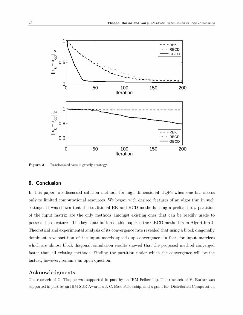
8.2. Experiment 2

For this experiment, we chose n = 1024. We first generated an arbitrary matrix V ∈ Rn×n using

the rule V =Z1024 and then constructed the matrix P using the relation P = V tV. We then chose

a subset τ ⊂ [n] made of 32 arbitrary indices. The rows and columns of P corresponding to τ were

multiplied by 1000 to finally get the P matrix. Note that, since n was only 1024, we stored all the

above matrices in their entirety directly in the main memory. Finally we generated an arbitrary

xopt and built q using the relation q= Pxopt.


We solved a UQP with this P and q using three methods: Strohmer and Vershynin’s randomized

Kaczmarz, Leventhal and Lewis’ randomized coordinate descent and the proposed GBCD. We

implemented the GBCD method using Algorithm 4 with Π≡ {π1, . . . , π1024} where each πi = {i}.

That is, each Pπi is made of one row of P. Since the input matrix P was small enough to be retained

in the main memory, we skipped all the steps of this algorithm that involved secondary storage

reads. The computation of the inverses in the preprocessing step was also skipped. The randomized

coordinate descent was implemented in exactly the same manner as the GBCD method except for

the block selection strategy. In each iteration of the randomized BCD, the blocks from Π (rows

of P in this case) were chosen using a distribution that was proportional to the diagonal entries

of P. Along similar lines, we implemented the randomized Kaczmarz method using Algorithm 1.

Specifically, the strategy ζb used was to select the blocks of the partition Π using a distribution

that was proportional to the square of || · ||2 norm of the rows. All the methods started out at the

origin. The comparative performance of these methods is given in Figure 2. The three methods are

denoted using RK, RCD and GBCD. Clearly, under both the norms || · ||2 and || · ||P , the GBCD

method has faster convergence. But the key thing to observe is that the decrease in error under

|| · ||2 norm for the randomized approaches is almost negligible. This happens mainly because of

the way the P matrix was constructed and the way the randomized methods work. In particular,

note that both these methods sample almost always only those rows of P that have large mass,

i.e., the rows of the row submatrix Pτ , irrespective of where the current estimate is. Because of

this, the estimates of the Kaczmarz algorithm lie very close to the subspace span(Pτ ). In similar

fashion, the estimates of the coordinate descent algorithm lie very close to the subspace span(Iτ ).

From these observation, it is easy why the || · ||2 norm convergence of the error for these methods

is poor. The proposed method, however, is adaptive and hence is able to overcome these problems.

8.3. Experiment 3

In this experiment, we chose n = 1024 and generated the P ∈ Rn×n matrix and q ∈ Rn vector in

exactly the same manner as we did in Experiment 2. We then solved a UQP with this P matrix

and q vector as input using the proposed GBCD method in two different ways. Specifically, we

chose two different input partitions. In the first way, we arbitrarily partitioned the rows of P into

32 blocks with each block made up of 32 rows. In the second way, we kept all the 32 rows with

large numbers, i.e., rows with indices in τ, in one block while the remaining rows were arbitrarily

partitioned into 31 blocks with each block again made up of 32 rows. In a loose sense, we tried to

use a block diagonally dominant partition of P. The starting point in both ways was the origin.

The performance of GBCD with these two different partitions as input is given in Figure 3. As one

can see, the performance was better with the block diagonally dominant partition.


0 50 100 150 2000

0.5

1

Iteration

||xk −

xop

t|| P

RBKRBCDGBCD

0 50 100 150 200

0.6

0.8

1

Iteration

||xk −

xop

t|| 2

RBKRBCDGBCD

Figure 2 Randomized versus greedy strategy.

9. Conclusion

In this paper, we discussed solution methods for high dimensional UQPs when one has access

only to limited computational resources. We began with desired features of an algorithm in such

settings. It was shown that the traditional BK and BCD methods using a prefixed row partition

of the input matrix are the only methods amongst existing ones that can be readily made to

possess these features. The key contribution of this paper is the GBCD method from Algorithm 4.

Theoretical and experimental analysis of its convergence rate revealed that using a block diagonally

dominant row partition of the input matrix speeds up convergence. In fact, for input matrices

which are almost block diagonal, simulation results showed that the proposed method converged

faster than all existing methods. Finding the partition under which the convergence will be the

fastest, however, remains an open question.

Acknowledgments

The research of G. Thoppe was supported in part by an IBM Fellowship. The research of V. Borkar was

supported in part by an IBM SUR Award, a J. C. Bose Fellowship, and a grant for ‘Distributed Computation


0 50 100 150 2000

0.5

1

Iteration

||xk −

xop

t|| P

Arbitrary PartitionGood Partition

0 50 100 150 2000

1.5

3

Iteration

||xk −

xop

t|| 2

Arbitrary PartitionGood Partition

Figure 3 Choosing a good partition.

for Optimization over Large Networks and High Dimensional Data Analysis’ from the Department of Science

and Technology, Government of India. A portion of this work was done when G. Thoppe did a summer

internship at IBM with D. Garg.

References

Bertsekas, Dimitri P, John N Tsitsiklis. 1989. Parallel and distributed computation: numerical methods.

Prentice-Hall, Inc.

Bland, Robert G, Donald Goldfarb, Michael J Todd. 1981. The ellipsoid method: a survey. Operations

research 29(6) 1039–1091.

Bo, L., C. Sminchisescu. 2008. Greedy Block Coordinate Descent for Large Scale Gaussian Process Regres-

sion. Uncertainty in Artificial Intelligence.

Boyd, Stephen, Neal Parikh, Eric Chu, Borja Peleato, Jonathan Eckstein. 2011. Distributed optimization

and statistical learning via the alternating direction method of multipliers. Foundations and Trends in

Machine Learning 3(1) 1–122.

Davis, Timothy A. 2006. Direct methods for sparse linear systems, vol. 2. SIAM.


Demmel, James W. 1988. The probability that a numerical analysis problem is difficult. Mathematics of

Computation 50(182) 449–480.

Deutsch, Frank. 1985. Rate of convergence of the method of alternating projections. Parametric optimization

and approximation. Springer, 96–107.

Deutsch, Frank, Hein Hundal. 1997. The rate of convergence for the method of alternating projections, II.

Journal of Mathematical Analysis and Applications 205(2) 381–405.

Eldar, Yonina C, Deanna Needell. 2011. Acceleration of randomized Kaczmarz method via the Johnson–

Lindenstrauss Lemma. Numerical Algorithms 58(2) 163–177.

Elfving, Tommy. 1980. Block-iterative methods for consistent and inconsistent linear equations. Numerische

Mathematik 35(1) 1–12.

Galantai, A. 2005. On the rate of convergence of the alternating projection method in finite dimensional

spaces. Journal of mathematical analysis and applications 310(1) 30–44.

Glasmachers, Tobias, Urun Dogan. 2013. Accelerated coordinate descent with adaptive coordinate frequen-

cies. Asian Conference on Machine Learning . 72–86.

Golub, Gene H, Charles F Van Loan. 2012. Matrix computations, vol. 3. JHU Press.

Hildreth, Clifford. 1957. A quadratic programming procedure. Naval research logistics quarterly 4(1) 79–85.

Kaczmarz, Stefan. 1937. Angenaherte auflosung von systemen linearer gleichungen. Bulletin International

de lAcademie Polonaise des Sciences et des Lettres 35 355–357.

Kelley, James E, Jr. 1960. The cutting-plane method for solving convex programs. Journal of the Society

for Industrial & Applied Mathematics 8(4) 703–712.

Kolda, Tamara G, Robert Michael Lewis, Virginia Torczon. 2003. Optimization by direct search: New

perspectives on some classical and modern methods. SIAM review 45(3) 385–482.

Leventhal, Dennis, Adrian S Lewis. 2010. Randomized methods for linear constraints: Convergence rates

and conditioning. Mathematics of Operations Research 35(3) 641–654.

Levin, A Yu. 1965. On an algorithm for the minimization of convex functions. Soviet Mathematics Doklady ,

vol. 160. 1244–1247.

Loshchilov, Ilya, Marc Schoenauer, Michele Sebag. 2011. Adaptive coordinate descent. Proceedings of the

13th annual conference on Genetic and evolutionary computation. ACM, 885–892.

Needell, Deanna, Joel A Tropp. 2014. Paved with good intentions: Analysis of a randomized block kaczmarz

method. Linear Algebra and its Applications 441 199–221.

Nelder, John A, Roger Mead. 1965. A simplex method for function minimization. Computer journal 7(4)

308–313.

Nesterov, Yu. 2012. Efficiency of coordinate descent methods on huge-scale optimization problems. SIAM

Journal on Optimization 22(2) 341–362.


Richtarik, Peter, Martin Takac. 2012. Parallel coordinate descent methods for big data optimization. arXiv

preprint arXiv:1212.0873 .

Strohmer, Thomas, Roman Vershynin. 2009. A randomized kaczmarz algorithm with exponential conver-

gence. Journal of Fourier Analysis and Applications 15(2) 262–278.

Warga, Jack. 1963. Minimizing certain convex functions. Journal of the Society for Industrial & Applied

Mathematics 11(3) 588–593.

Wright, SJ, J Nocedal. 1999. Numerical optimization, vol. 2. Springer New York.

greedy block coordinate descent (gbcd) method for … block coordinate descent (gbcd) method for...

Documents