graduate aeronautical laboratories california institute...

GRADUATE AERONAUTICAL LABORATORIES CALIFORNIA INSTITUTE of TECHNOLOGY

Pasadena. California 91125

Chemical Reactions in Turbulent Mixing Flows

Paul E. Dimotakis*, James E. Broadwell*' and Anthony ~ e o n a r d i

Air Force Office of Scientific Research Grant No. 90-0304

Final Technical Report: Period ending 14 May 1992

15 July 1992

* Professor, Aeronautics Sr .4pplied Physics.

** Senior Scientist, .4eronautics.

t Professor, Aeronautics.

I REPORT DOCUMENTATION PAGE I OM# NO. o7ol.01~~ 1 f- ewowa

I - --

I I. r 6 W C Y at ONLY (Lean W J W (2. REPORT OAT( 13. REPORT TYPE A N 0 OATES COVERLO

1 15 J u l y 1992 1 F i n a l : 15 May 1991 - 14 May 1992 5. fUNOWG WUhuEIIS I

7. PLIMIYWG on6*11~1nou NAME(S) AND CS(MLSS(ES) L PERFOIIM~WG ORGANPI~ON C a l i f o r n i a I n s t i t u t e of Technology RErnRT WUMIER

Chemical Reac t i ons i n Turbu len t Mixing Flows

'

Ll(rrH- P a u l E. Dimotakis James E. Broadwell Anthony Leonard

-- G r a d u a t e A e r o n a u t i c a l L a b o r a t o r i e s M a i l S t o p 301-46 Pasadena , CA 91125

PE - 6110ZF E'R - 2308 S A - E 3 s G - AFOSR-90-0304

I 9. SKWOCI(GIYON(T0RWG AGENCY NAME(S) AN0 A W S H E S ) 10. SK)NSOMLGIMONl?ORIYG

A ~ O S R / N A A G E I K I REPORT WMILR

I .

B u i l d i n g 410 B o l l i n g AFB DC 20332-6448

I lab. MSTIIPUIIOII COOE 1 Approved f o r p u b l i c release: d i s t r i b u t i o n is I I u n l i m i t e d

The purpose of this research is to col~duct fundamental investigations of turbulent mixing, chemical reaction and combustion processes in turbulent, subsonic and supersonic flows. Our approach has been to carry out a series of detailed theoretical and experimental studies of turbulent mixing in both free shear layers and axisymmetric jets. To elucidate molecular transport effects, experiments and theory concern themselves with both reacting and non-reacting flows of liquids and gases, in fully-developed turbulent flows,%.c., in moderate to high Reynolds number flows. The computational studies are, at present, focused at fundamental issues pertaining to the computational simulatioli of both compressible and incompressible flows. Modeling has been focised on both shear layers and turbulent jets, with an effort to include the physics of the molecular transport processes, as well as formulations of models that permit the full chemical kinetics of the combustion process to be incorporated. Our primary diagnostic development efforts are currently focused on data-acquisition electronics to meet very high-speed, high-volume data requirements, the acquisition of single, or a sequence, of two-dimensional images, and the acquisition of data from arrays of supersonic flow sensors. Progress has also been made in the development of a dual-beam laser interferometer/correlator to measure convection velocities of large scale structures in slipersonic shear layers and in a new method to acquire velocity field data using pairs of scalar images closely spaced in time.

Turbulence, s h e a r Layers , j e t s , mixing, 15. N U M I E I Of PAGES 75

combust ion, numer ica l s i m u l a t i o n , f r a c t a l s , t u r b u l e n t mixing modeling, ve loc ime t ry 16. PMI C O M

U n c l a s s i f i e d I U n c l a s s i f i e d I U n c l a s s i f i e d I UL I I 1 I

-

I Sundard Form 290 ((IOOlQP O n W - * uY u s t * n M 1

The purpose of this research is to conduct fundamental investigations of turbulent mixing, chemical reaction and combustion processes in turbulent, subsonic and supersonic flows. Our program is comprised of several parts:

a. an experimental effort,

b. an analytical effort,

c. a computational effort,

d. a modeling effort,

and

e. a &agnostics development and data-acquisition effort,

the latter as dictated by specific needs of the experimental part of the overall pro-

gram.

Our approach has been to carry out a series of detailed theoretical and experimental studies of turbulent mixing in primarily in two, well-defined, fundamentally important flow fields: free shear layers and axisymmetric jets.

To elucidate molecular transport effects, experiments and theory concern themselves with both reacting and non-reacting flows of liquids and gases, in fully-

developed turbulent flows, i.e., in moderate to high Reynolds number flows. The computational studies are, at present, focused at fundamental issues pertaining to the computational simulation of both compressible and incompressible flows. Mod- eling has been focused on both shear layers and turbulent jets, with an effort to

include the physics of the molecular transport processes, as well as fornlulations of models that permit the full chemical kinetics of the combustion process to be

incorporated. Our primary diagnostic development efforts are currently focused

on data-acquisition electronics to meet very high-speed, high-volume data require-

ments, the acquisition of single, or a sequence, of two-dimensional images, and the acquisition of data from arrays of supersonic flow sensors. Progress has also been

made in the development of a dual-beam laser interferometer/correlator to measure convection velocities of large scale structures in supersonic shear layers and in a new

method to acquire velocity field data using pairs of scalar images closely spaced in time.

1. Int roduct ion

We have made progress under the sponsorship of this Grant, for the period

ending 14 May 1992, in several areas. A review paper documenting much of the

work at Caltech in shear layer mixing and combustion in the last ten years, or so,

has appeared as Chapter 5 in the High-Speed Flight Propulsion Systems, Volume 137 of the AIAA Progress Series in Astronautics and Aeronautics (Dimotakis 1991).

Copies are available on request.

In our experimental effort in supersonic shear layers, we have increased the high-speed stream Mach number to 2.5 and performed a first set of exploratory

investigations at this higher compressibility condition. We have also performed a first set of experiments in the transonic shear layer regime.

i In our investigations of turbulent jets,+ two theses are now available, An Exper-

imental Investigation of Chemically-Reacting, Gas-Pl~ase Turbulent Jets (Gilbrech

1991), that explored Reynolds number effects on turbulent flame length and the

influence of buoyancy on turbulent jet flames; and Mixing in High Schmidt Aium- ber Turbulent Jets (Miller 1991), that examined Reynolds number effects, Schmidt

number effects, and the influence of initial conditions on the turbulent jet's mix-

ing behavior. Progress has also been made in understanding buoyancy effects in

turbulent jets, with an eye in understanding the mixing enhancement that we have documented occurs under certain conditions. Finally the development of jet mixing models that permit the inclusion of full chemical kinetics calculations has also pro- gressed, with considerable improvements in the quantitative descriptions of a host of phenomena, including NO, production by turbulent jet flames.

In our analytical/computational effort, we are developing new, reliable methods for computing interactions of shock waves and other discontinuous waves that may arise in multidimensional, unsteady compressible flows.

In our diagnostics effort, we are continuing our progress with a new generation of high-speed, high-volume data acquisition systems, with the development of a new two-beam laser correlator to measure turbulent structure convection velocities, and

a new method to measure velocity field information from pairs of images.

: The investigations of turbulent mixing and combustio~l in turbulent jets are co-sponsored by the Gas Research Institute.

2. Mixing a n d combustion in supersonic, tu rbulent shear layers

Some preliminary runs were made during the last year at a high-speed stream Mach number of 2.5 and at compressible but subsonic flow conditions. Both of these showed new and interesting phenomena. However, on 28 June 1991, the Sierra Madre earthquake caused a major disruption to the Supersonic Shear Layer (S3L) combustion facility. The high pressure tank seal developed a leak, forcing a

significant design reevaluation and repair effort. While that effort was in progress, a new instrument designed to measure large-scale-structure convection velocities was being developed. These are important for modeling chemically reacting shear

layers.

2.1 Preliminaries at Mach 2.5

The expansion of the operating range of the facility to a high-speed stream

Mach number of 2.5 was begun in May 1991 with Dr. Jeffery Hall. This work was left in the preliminary stage due to several factors; the discovery of a flaw in the

original design of the S3L test section splitter plate and the earthquake damage to the high speed supply tank. Despite these shortcomings, significant new information was gleaned from these preliminary runs. Based on previous experience, the growth

rate of these cases should be very close to runs at ideal conditions; additionally, the

structures indicated by the travelling waves are a robust manifestation of supersonic

convection velocities of turbulent structures with respect to the shear layer free streams.

The new MI = 2.5 [Nz] runs provide highly compressible flows with a different density ratio from our previous A41 = 1.55 [He] runs (Hall 1991). These flows have similar isentropic convective Mach numbers with respect to each stream. Both runs

exhibit travelling waves in the low-speed stream, but the wave speeds are different, due, in large part, to the lower (absolute) speed of the MI = 2.5 [Nz] stream

(U1 = 600m/s), as opposed to the A41 = 1.55 [He] stream (Ul = 1100m/s). The normalized growth rates also are consistent (for the most part) with the established body of data, at this time, except for the N2/Ar case. The latter, however, was

found to have a non-zero pressure gradient. Although the lowest compressibility

case seems to have a low normalized growth rate, this was not unexpected. By this criterion, it is similar to the low density ratio cases from previous experiments at

MI N 1.5.

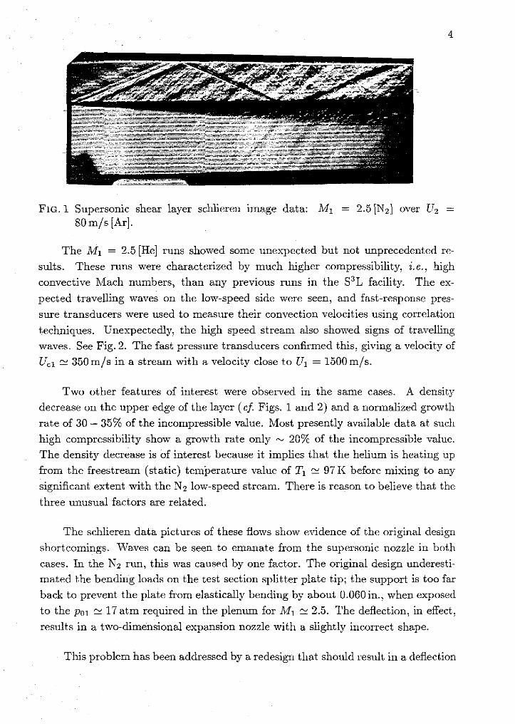
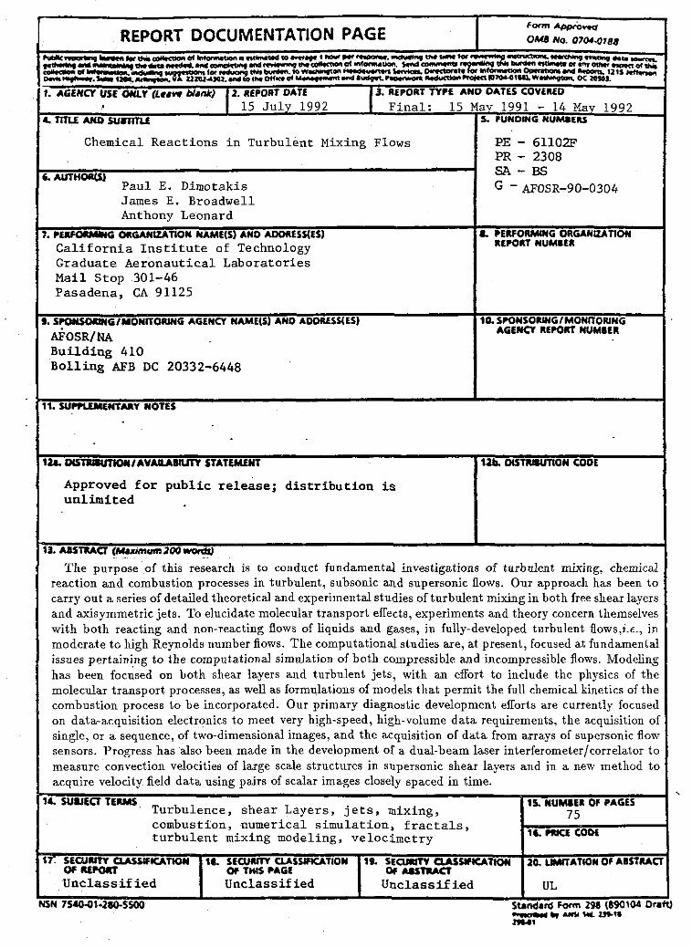
FIG. 1 Supersonic shear layer schlieren image data: Ml = 2.5[N2] over U2 = SO m/s [As].

The MI = 2.5 [He] runs showed some unexpected but not unprecedented re-

sults. These runs were characterized by much higher compressibility, i.e., high convective Mach numbers, than any previous runs in the S3L facility. The expected travelling waves on the low-speed side were seen, and fast-response pres-

sure transducers were used to measure their convection velocities using correlation

techniques. Unexpectedlj~, the high speed stream also showed signs of travelling waves. See Fig. 2. The fast pressure transducers confirmed this, giving a velocity of Ucl -- 350m/s in a stream with a velocity close to [TI = 1500m/s.

Two other features of interest were observed in the same cases. A density decrease on the upper edge of the layer (cf. Figs. 1 and 2) and a normalized growth

rate of 30 - 35% of the incompressible value. Most presently available data at such high compressibility show a growth rate only - 20% of the incompressible value. The density decrease is of interest because it implies that the helium is heating up from the freestream (static) temperature value of TI -. 97I< before mixing to any significant extent with the N2 low-speed stream. There is reason to believe that the

three unusual factors are related.

The schlieren data pictures of these flows show evidence of the original design

shortcomings. Waves can be seen to emanate from the supersonic nozzle in both cases. In the N2 run, this was caused by one factor. The original design underesti- mated the bending loads on the test section splitter plate tip; the support is too far

back to prevent the plate from elastically bending by about 0.060in., when exposed to the pol 1. 17 atm required in the plenum for &Il -. 2.5. The deflection, in effect,

results in a two-dimensional expansion nozzle with a slightly incorrect shape.

This problem has been addressed by a redesign that should result in a deflection

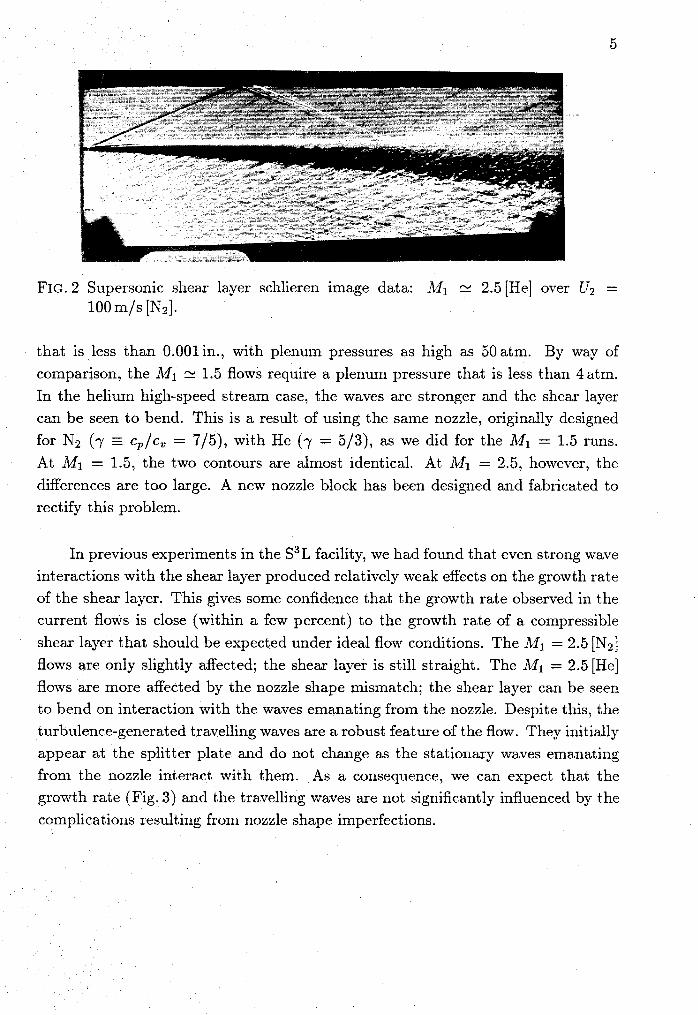
FIG. 2 Supersonic shear layer schlieren image data: Ml E 2.5 [He] over U2 = 100 m/s INz].

that is less than 0.001 in., with plenum pressures as high as 50 atm. By way of comparison, the A& cx 1.5 flows require a plenum pressure that is less than 4atm. In the helium high-speed stream case, the waves are stronger and the shear layer can be seen to bend. This is a result of using the same nozzle, originally designed for N2 (y = cp/c, = 7/5), with He (y = 5/3), as we did for the MI = 1.5 runs.

At MI = 1.5, the two contours are almost identical. At MI = 2.5, however, the differences are too large. A new nozzle block has been designed and fabricated to rectify this problem.

In previous experiments in the S3L facility, we had found that even strong wave interactions with the shear layer produced relatively weak effects on the growth rate of the shear layer. This gives some confidence that the growth rate observed in the current flows is close (within a few percent) to the growth rate of a compressible shear layer that should be expected under ideal flow conditions. The MI = 2.5 [Nz]

flows are only slightly affected; the shear layer is still straight. The = 2.5 [He] flows are more affected by the nozzle shape mismatch; the shear layer can be seen to bend on interaction with the waves emanating from the nozzle. Despite this, the turbulence-generated travelling waves are a robust feature of the flow. They initially appear at the splitter plate and do not change as the stationary waves emanating

from the nozzle interact with them. As a consequence, we can expect that the growth rate (Fig. 3) and the travelling waves are not significantly influenced by the complications resulting from nozzle shape imperfections.

1.0 m Y I I I

++ P a p a m 0 S ~ h 0 ~ 6 Roshko (1988) 0 Chinzei et al. (1986)

FIG. 3 Compressible shear layer normalized growth rate data: New A!fl = 2.5 and subsonic runs, as well as previous data.

.8

. 4

.2

2.2 Co~npressible subsonic shear layer Rows

- A Clemens 6 Mungal (1990) 0

- + Hall (1991)

++go 0 Mach 2.5 He runs

+ M A Mach 2.5 N2 runs

. = - + 4 +o Compressible Subsonic runs -

- -

OP q 00

- a+ -

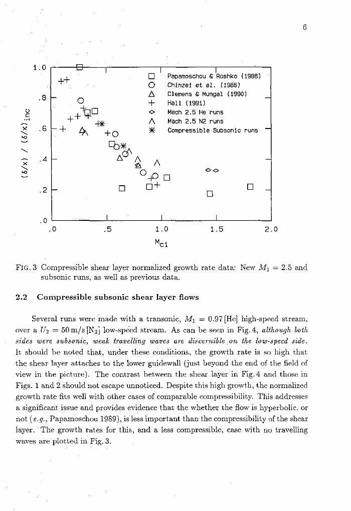
Several runs were made with a transonic, A!fl = 0.97 [He] high-speed stream, over a U2 = 50 m/s [Nz] low-spied stream. As can be seen in Fig. 4, although both

s ides were subsonic, weak travelling waves arc d i scerr~ ib le O T L the low-speed s ide .

It should be noted that, under these conditions, the growth rate is so high that the shear layer attaches to the lower guidewall (just beyond the end of the field of view in the picture). The contrast between the shear layer in Fig. 4 and those in

Figs. 1 and 2 should not escape unnoticed. Despite this high growth, the normalized growth rate fits well with other cases of comparable compressibility. This addresses a significant issue and provides evidence that the whether the flow is hyperbolic, or

not (e.g., Papa~noschou 1989), is less important than the compressibility of the shear layer. The growth rates for this, and a less compressible, case with no travelling waves are plotted in Fig. 3.

FIG. 4 Transonic shear layer schlieren image data: MI = 0.97[He], over Uz = 50 m/s [Nz].

2.3 Recent ear thquakes a n d required repairs

Work on both the efforts described above was interrupted by a major repair

job necessitated by the June 1991 Sierra Madre earthquake. After discovering the

leak, we were forced to stop experiments. In addition to considering simply re- placing the seal, other alternatives were investigated. These alternatives included remanufacturing the tank to eliminate the large 36 in. flange. Unfortunately, the

necessity of including the high heat capacity aluminum packing to prevent a sig-

nificant stagnation temperature drop in the high speed stream, in the course of a run, prevented the most favorable resolution; the heat-treating temperature of the

welds (as required by the high pressure vessel code for hydrogen-capable tanks) is

too close to the melting temperature of aluminum.

In the end, we decided to replace the seal, with several steps taken to minimize

the probability of future problems. Specifically, the seal material was changed to

one that gives the closest coefficient of thermal expansion to minimize thermal

stresses when the tank heating is activated. In addition, a ultrasonic measuring device was used, in retorquing the large flange bolts, to ensure that a uniform

and sufficient tension was placed on the bolts. This should give the best chance to prevent damage from any future event by giving us a level of consistency which could not be obtained merely by tightening to a fixed torque. For better or for worse, we had the opportunity to test this. Following the recent Landers earthquake (28 June 1992, magnitude 7.4, 90 miles east of Pasadena) and long sequence of strong

aftershocks, we loaded the large tank to working pressure with helium. No leaks were found using a sensitive helium leak detector.

2.4 .Design of a new i~ls t ru~l le i l t

At this time, travelling waves provide us with the only means of measuring the turbulent structure(s) convection velocity. Accurate chemical kinetic modelling of the reacting shear layer depends significantly upon this velocity as it determines the

time of flight and also enters in the modeling of the entrainment ratio. Specifically, a higher velocity gives a shorter time for reactions and thus raises the required concentrations/temperatures for fast chemistry. A relative velocity ratio with respect

to the two freestreams provides an asymmetric entrainment environment. There is a possibility that the wave velocity might not be the only velocity in the shear layer;

if the wave velocity is not the fluid velocity, then a model based on the wave velocity could be significantly wrong. For this reason, a new instrument was designed to measure density (index of refraction) interface convection velocities. This should be able to measure both the fluid velocity and wave velocities, whether they ars the

same or different.

3. Mixing a n d coinbustioil in tu rbu len t je ts

The research effort on turbulent jet mixing, involving both the gas-phase, chemically reacting and liquid-phase, non-reacting jet investigations, is cosponsored by

the Gas Research Institute, GRI Contract No. 5087-260-1467.

3.1 Gas-phase chemically reacting j e t investigations

The results described below are from the Ph.D. thesis by Gilbrech (1991) that

was completed during the last year (copies are available on request). A paper

describing some of the work (Gilbrech & Dimotakis 1992) is included as -4ppendix B of this report. The experimental investigations reported in the thesis investigate

a steady, effectively unconfined, chemically-reacting turbulent jet issuing into a quiescent reservoir. The Reynolds nunlber (based on the nozzle exit diameter) is varied through pressure, i.e., density, with the jet exit velocity and exit diameter held constant. The time-averaged line integral of temperature, measured along the transverse axis of the jet by the wires, displays a logarithmic dependence on z l d *

within the flame zone, and asymptotes to a constant value beyond the flame tip. The main result of the work is that the flame length, as estimated from the temperature

measurements, varies with changes in Reynolds number, suggesting that the mixing process is not Reynolds number independent up to Re = 1.5 x 10'. Specifically, the normalized flame length L r / d * displays a linear dependence on the stoichiometric mixture ratio 4, with a slope that decreases from Re N 1.0 x lo4 to Re N 2.0 x lo4 ,

and then remains constant for Re > 2.0 x 10% Additionally, the measurements revealed a "mixing virtual origin," defined as the fas-field flame length extrapolated to 4 = 0, that increases with increasing Reynolds number, for Re 5 2.0 x lo4 and

then decreases with increasing Reynolds number for Re > 2.0 x lo4.

The chemically reacting jet experiments were performed at a Damkohler num-

ber greater than 5.2, a value found to be the threshold to the fast chemistry regime.

To insure that the turbulent jets investigated were momentum dominated to the farthest measuring station, a separate set of experilnents was performed. In these

experiments, the adiabatic flame temperature ATf was raised to ~vl-here buoyancy

affected the product thicliness 6p distribution and the logarithmic dependence on

x l d * of the time-averaged line integral of temperature no longer held. Under these conditions, it was found that molecular mixing is enhanced.

3.1.1 Stoichiometric mixture ratio and Reynolds ilumber effects

All runs were performed at pressures between 1 atm 5 p 5 15 atm. The jet gas was always Fz in a Nz diluent and the reservoir gas was always NO in a Nz diluent.

Experiments at four stoichiometric mixture ratios, 4, were performed at each

Reynolds number to produce four different flame lengths. In this study, 4 is defined

in the usual manner as the mass fraction of Fz in Nz, divided by the mass fraction

of NO in N2, normalized by the corresponding stoicl~ioinetric mass fraction ratio,

2.e..

where the mass fraction, E;, is defined for a mixture of N species, as

and

mi = mass of the it" species

The adiabatic flame temperature rise ATf for each , was computed using the CHEMIUN chemical kinetics program (Kee et al. 1980). The four values of dJ with the corresponding mass fractions and ATi's are given in the following table.

The choice of 4Ti was determined from several preliminary experiments. The lomlest value of ATr that could be measured accurately and with repeatability was

sought to reduce both buoyancy effects and heat release effects on the flow dynamics. The choice of ATf 7 I<, on the basis of buoyancy concerns, will be developed below.

Table 1: Stoichiometric mixture ratios, mass fractions, and adiabatic flame temperature rises.

dJ 7.0

10.0 14.0 17.9

1 ' ~ ~ 0.0127 0.0174 0.0237 0.0300

I/N o 0.0029 0.0028 0.0027 0.0027

4Tr (10 7.2 6.9 6.9 6.7

FIG. 5 Normalized product thickness versus loglo(x/d*) for the various 4's.

Figure 5 shows the data for the 4 = 7, 10, 14, and 18 runs. The solid line is a compound curve fit with a linear least squares fit in the ramp region and a cubic spline fit to the knee region. ~ h k runs were fairly repeatable as shown by the good agreement of the repeated runs. All of the runs exhibit a linear ramp region when plotted in semi-logarithmic coordinates and a nearly constant asymptotic level after the knee or flame tip region. The average flame lengths were estimated from these

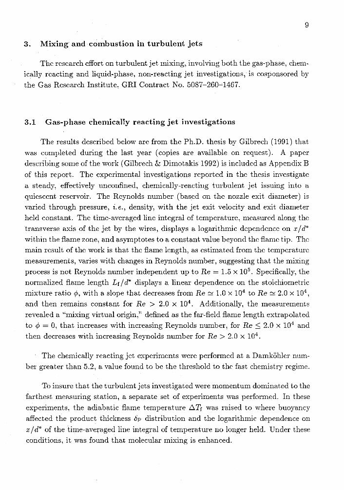
curves by determining the 99% of maximum ~ P / L , point. These flame lengths are plotted versus 4 for the various Reynolds numbers in Fig. 6. The straight lines are linear least-squares fits to the data of the form

where 4 and B are functions of Re with A being the slope and B being defined

as the "mixing virtual origin". This mixing virtual origin is a new observation and

corresponds to the abscissa-intercept in Fig. 6, z.e., the flame length extrapolated

to 4 = 0. If the flow could be described by its far-field behavior at the nozzle exit,

FIG. 6 Normalized flame length versus 4,

then B would be the flame length measured in the limit of 4 7- 0. The variation

of B in Fig. 6 indicates that this mixing virtual origin systelnatically decreases with increasing Reynolds number for Re 2 2.0 x lo4. Some of the variation in B could be attributable to the uncertainty in the curve fits used for the flame length determination. Another possibility could be a variation in xo, the virtual origin of the jet, with increasing Re. However, even combined, these effects are not large enough to explain such a large variation in B. A nonzero intercept in itself is not surprising, if one realizes that the potential core extends roughly six diameters from

the nozzle exit and that the self-similar region of the jet typically begins around

x / d o = 20 (e.g., Dowling & Dimotakis 1990). Therefore, fully-developed turbulent mixing on a molecular scale requires some distance downstream of the nozzle exit to develop, hence the streamwise delay in molecular mixing. The fact that B has

such a large value and that it varies with Re, ho\vever, is a new observation.

13

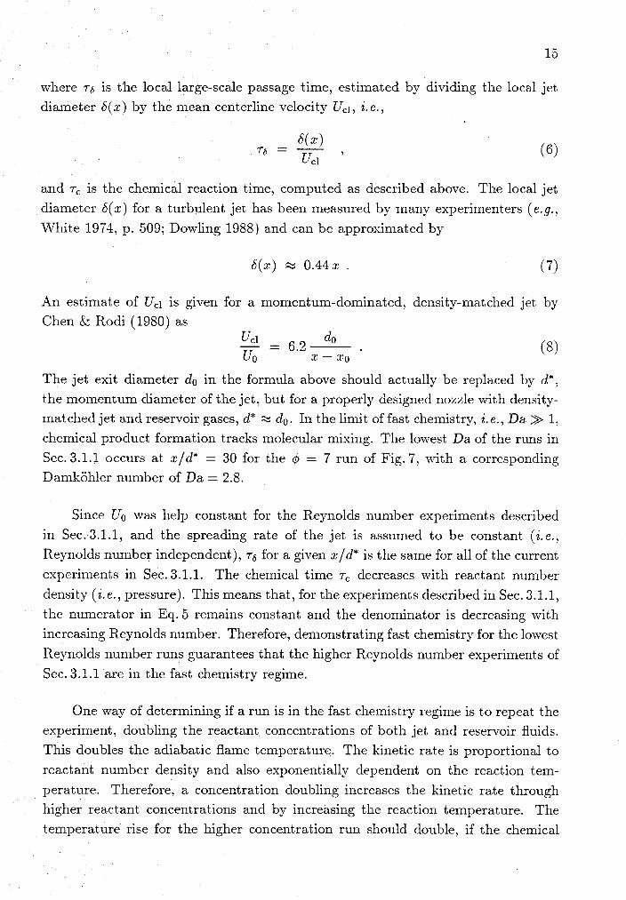
3.1.2 Kinetics

The Fz/NO chemistry in this study can be described by the "effective" reaction:

# = 7 . 0 . rC = 0.91 msec

= 0.68 msec

= 14.0. = 0.49 rnsec . . - - . . - = 17.9. = 0.40 msec

FIG. 7 Chemical reaction times for some of the runs described in Sec. 3.1.1, p =

1 atm, T = 293 I<.

The reaction actually consists of two chain reactions of different rates and heat of reaction. To estimate the chemical reaction time T,, these reactions were investi-

gated using the CHEMI<IN chemical kinetics software (Kee e t al. 19S0) with a constant-mass, constant-pressure reactor. Figure 7 shows a sample result from the program for the mass fractions corresponding to the four 4's used in Sec. 3.1.1.

FIG. 8 Temperature doubling to check kinetic rate, 4 = 7, Uo = 62.4m/s. Dam- kohler number is given for x/d* = 30.

3 J \ a

w

The reaction time T, was determined by drawing a tangent to the curve at

its steepest point and using the intersection of this tangent line with the adiabatic

flame temperature as the chemical time. The slowest rate is for 4 = 7, p = 1 atm with rC = 0.91 msec.

-02

For these experiments, it was required that the time lag between molecular mixing and chemical product formation be negligible. In this mixing-limited con-

A Re = 10,000, ATf = 3.6 K. p = 1 a t m . Da = 1.4

- = 10,000, = 7.2 K. = 1 a t m . = 2.8 - + = 10,000. = 14.4 K, = 1 a t m . = 5.9

m = 150.000, = 7.2 K. = 15 atm. = 43.0

dition, that we will designate as the fast chemistry regime, there is a one-to-one

correspondence between molecular mixing and product formation. The ratio of the

local large-scale passage time to the chen~ical.reaction time is one way of estimat- ing when the reacting flow is in the fast chemistry regime. This ratio of these two

quantities is (one of) the Damkohler number(s), defined by

- - Re = 28.000, # = 7

Uo = 62.4 rn/s, p = 2 atrn

- AT^ = 7.2 K . Da = 5.6 - o = 14.4 K. = 11.8

A = 28.6 K , = 25.6

I I I I I

FIG. 9 Temperature doubling to check kinetic rate. Damkohler number is given for xld* = 30.

product formation is already mixing-limited. If the chemistry was not fast before

the concentration doubling, the faster kinetic rate after the doubling should result in more than double the chemical product and, correspondingly, more than double the temperature rise.

A similar temperature doubling was performed for the run in Sec. 3.1.1 with

the lowest Damkohler number, shown in Fig. 8. These data do not collapse. Slow chemistry should oilly affect the ramp region of the curve and possibly result in a longer flame length. The asymptotic level, however, should eventually agree

at some downstream location because all of the F2 should react if one goes far

enough downstreanl. The asymptotic level does not agree for the various ATi1s.

The asymptotic level nearly doubles for each temperature doubling leading to the hypothesis that some of the F2 was being depleted by passivation of the nozzle

plenum screens and honeycomb during each run. -4t low concentrations, doubling

q5 = 14. A T f = 6.9 K . Uo = 62.4 m/s

+ R e = 10.000. p = 1 atm. Da = 5.2

# = 150,000. = 15 atm, = 85.0

I I I I I

FIG. 10 Runs showing the lowest Damkohler number that still demonstrates fast chemistry. Da is given for xld* = 30.

the absolute number of moles of F2, by doubling the reactant concentrations, should

reduce the passivation effect in half. This appears to be what is happening in Fig. 8, supporting the passivation hypothesis.

The kinetics and the pa.ssivation problems disappear for the run with ATf =

14.4 I< in Fig. 8, as demonstrated by the collapse of the data with the higher

Reynolds number run that should be in the fast chemistry regime.

Figure 9 shows the result of a similar experiment at p = 3 atm with two tem-

perature doublings. The collapse is good and. this condition appears to be in the fast chemistry regime with the ATf = 7.2 I< run having a Da = 5.6.

Figure 10 compares the run at p = 1 atm, 4 = 14, to the run at p = 15atm and the same 4 and flame temperature. This is the lowest value of the Damkohler

FIG. 11 Runs showing effects of slow chemistry in the ramp region, 4 = 10, ATf = 6.9 I<. Damkohler number given for x /d* = 30.

number in all of the experiments which still col1a.pses well with an experiment at

a much larger Damkohler number. The lower limit of Damlcohler number in these

experiments, in which the flow can be considered to be in the fast chemistry regime, is therefore Da. 21 5.2.

In the runs described thus far, the Dalnkoler number was changed by varying

the chemical time, but changing the large-scale passage time 7 s is another way of

varying Da. Several runs at different velocities and pressures were performed in which the Damkohler number was low but the temperature measurement beyond

the flame tip achieved the correct level, showing then1 to be free of passivation

problems. Figure 11 shows runs at various velocities and Damkohler numbers. The temperatures for the s1o.c~ chemistry conditions lag behind the fast chemistry

runs but eventually achieve the same level beyond the flame tip. This is how slow

chemistry was expected to manifest itself. The Damkohler nunlbers are consistent

with the limiting value of Da z 5.2 discussed above. The lower velocity runs show the effects of buoyancy beyond the flame tip. The high-velocity run is repeatable.

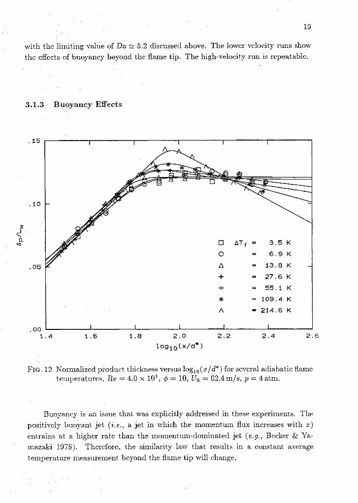
3.1.3 Buoyancy Effects

FIG. 12 Xormalized product thiclcness versus loglo (x/cl*) for several adiabatic flame temperatures, Re = 4.0 x lo", # = 10, Uo = 62.4m/s1 p = 4 atm.

Buoyancy is an issue that was explicitly addressed in these experiments. The positively buoyant jet (i.e., a jet in which the momentum flux increases with x)

entrains at a higher rate than the momentum-dominated jet (e .g . , Becker & Ya-

mazaki 1978). Therefore, the similarity law that results in a constant average temperature measurement beyond the flame tip will change.

The temperature excess beyond the flame tip is a conserved scalar obeying the

simiIarity law for a momentum-dominated jet. Therefore, the average temperature measurement will decay beyond the flame tip at some point when ljuoyancy forces

become comparable to the jet source momentum flux.

For the experiments described above, ATf was chosen by the requirement that the jet remain momentum-dominated up to the last measuring station at x /do =

240 for the 4's investigated. This was done by performing a set of preliminary experiments at several 4's. The longest flame length occurs at 4 = 17.9. This case was examined by systematically increasing ATf until the temperature measurement beyond the flame tip was no longer constant, but was observed to decrease. As

expected, the longest flame length is the most sensitive to buoyancy effects from temperature.

Figure 12 shows a set of experiments spanning adiabatic flame temperatures

ATf from 3.5 K to 215 K. A Reynolds number of 4.0 x lo4, was chosen for this scan. A 4 of 10 placed the flame tip in the center of the log,,(x/do) range, giving an equal number of points on each side of the knee. The temperature measurements beyond the flame tip reach a constant value for the low hea.t release runs, indicating that they are momentum-dominated. As the flame temperature increases, however, the temperature measurements no longer attain a constant level but begin to decrease with increasing xld*, as shown in Fig. 12, for ATf = 27.6 I<.

These data are presented here as a first effort to ascertain that the Reynolds number study was conducted in the momentum-dominated flow regime. This series of experiments showed an enhancement to molecular mixing under the influence of buoyancy. This enhancement depends on the relative effect of buoyancy to momentum forces. Further study of this behavior is currently in progress, as this effect plays an important role in the context of flow and mixing control.

3.2 Liquid-phase turbulent jet nlixiilg

During the past year, a thesis investigating the fine scale turbulent structure in a high Schmidt number (liquid phase) jet was completed (Miller 1991). Close to one hundred copies have been distributed to people throughout the world. Lim-

ited numbers are still available upon request. An additional publication related to

this work appeared in Physics of Fluids A (Miller & Dimotakis 1991b) during the reporting period (Appendix A of this report), and a third has been submitted for

publication (Miller & Dimotakis 1992). Seminars, lectures, and talks highlighting specific aspects of this work have been given by Paul Miller and Paul Dimotakis at ASU, Caltech, U. Chicago, UCSD, USC, at the Institute of Advanced Studies in Princeton, the DLR and Max Planck Institute (Gottingen, Germany), LLNL, the Sandia ST44R meeting, and the November 1991 meeting of the APS Division of Fluid Dynamics.

Results to date include an analysis of scalar interfaces for fractal properties (which differed substantially from previous reports in the literature), evidence of Taylor scales in the turbulent jet, and the absence of a I;-' region in the small scale region of this high Schmidt number flow - all of which have been discussed in previous reports. Important new observations concerning the applicability of fractal power-law ideas to turbulence have grown out of our work in that area, and a paper discussing the issue is included as Appendix C. This paper, in conjunction with Miller & Dimotakis (1991a), has changed how fractals are viewed in the Fluid Dynamics community.

Additional findings during this report period include additional new evidence that the jet pdf's, variance, and spectra vary with Reynolds namber, and that these changes with Re are also Schmidt number dependent. The long-time statistics of the jet concentration field were found to converge very slowly, scalar spectra were found not to obey the classical k - 5 / 3 power-law prediction, a log-normal behavior was discovered at small scales in the power spectra (with a starting point which scales like ~ e ~ / ~ ) , and initial conditions in the jet plenum and near the nozzle were seen to influence the flow's mixing behavior in the far-field.

In the following sections, we will describe some of these new findings in greater detail. For topics not covered here and for a. more complete documentation, the reader is directed to Dimotakis & Miller (1990)) Miller (1991), as well as Miller & Dimotakis (1991a,b and 1992).

3.2.1 Reynolds and Schmidt nunlber effects

An important result from these experiments is that the jet con'centration field changes with Reynolds number. Reynolds number for these jets is defined as

210 d R e r -, V

where uo is the jet exit velocity, d is the jet nozzle exit diameter, and v is the

kinematic viscosity of the fluid (water), and was va.ried in these experiments by altering uo. The jet concentration was measured on the centerline, and the probability density functions, or pdf's, were accumulated. The current results from the high Schmidt number jet, for a wide range of Re, are displayed in Fig. 13, along

with data from gas-phase jets (Dou~liag 1988).

.-.-.-.-.*

. . . . . . .. . . . . . . . . . ------ .--.--.-

circle and triangle

FIG. 13 Comparison of current pdf's with gas-phase results from Dowling (1988).

As is apparent in Fig. 13, the high Schinidt number pdf's become taller and

narrower with increasing Re, while the gas-phase pdf's vary little. It should be noted that a narrower pdf implies a mixture with a more uniform concentration,

i.e., more homogeneous o r well-mixed. Therefore, we conclude that the behavior

of the pdf's in Fig. 13 suggests that the liquid-phase jet is less well mixed than the gas-phase jet, but that this difference decreases with increasing Re: Alternatively, the gas-phase composition is relatively insensitive to Re, while the liquid-phase jet becomes better mixed with increasing Re.

Another, related, measure of the misedness of the jet is the scalar, or concentration, variance defined as

(cf. Miller & Dimotakis 1991b), where c,,, is the highest concentration present and p(c) is the probability density function of the jet fluid concentration c, normalized such that

The variance is typically nondimensionalized by the mean squared, z2. The resulting quantity is a measure of the width of the distribution p(c/7), i. e., pdf's such as in Fig. 13. Just as a narrower pdf indicates a better mixed jet, smaller variance values imply more uniform composition, with a perfectly homogeneous, constant concentration having a variance of zero. The concentration variance was calculated from the jet concentration data over a range of Reynolds numbers. The results are compared with the gas-phase results in Fig. 14.

The high Schmidt number points are fit with a function chosen for its simplicity, ability to approximate the observed behavior, and capability to either a.pproacl1 a nonzero asymptotic value (or zero, if it were indicated). The fit does suggest that the points are approaching a const ant value with increasing Reynolds number, and the determined asymptote, 0.039, is in good agreement with the finding from the analysis of previous data of 0.04 (Miller & Dimotakis 1991b), as discussed further in Miller (1991).

The observed decrease of the concentration variance (or, equivalently, the rms) in the high Schmidt number jet is a substantial effect. The jet becomes better mixed, apparently approaching an asymptotic, high Reynolds number value of the variance and a similarity in the concentration pdf's. In a span of 1.5 decades in Reynolds number, the variance is reduced by over 70%. The decline is not from deteriorating resolution, as discussed both in Miller & Dimotakis (199lb) and Miller (1991).

current work (Phase 11) gas-phase (Dowl. &Dimo. 1990) f i t of A + B ( R ~ ) P

(Ae0.039, B=24 .8 , p=-0.647)

FIG. 14 Comparison of variance values with gas-phase results of Dowling & Dimo- takis (1990).

Like the pdf's, the gas-phase variances measured by Dowling (1988) change little over the range of Reynolds numbers investigated, indicating a fundameiltal dif-

ference between the order unity Schmidt number (gas-phase) and the high Schmidt number (liquid-phase) jet mixing. This difference is also reflected in the behavior of the corresponding power spectra for the two cases. Figure 15 displays selected concentration power spectra from the current work, with the results of Dowling (1988) for comparison.

The high Sc spectra have a considerabiy greater extent than the order unity Sc spectra at the high frequencies. This behavior is expected in view of a species diffusion scale that is smaller than the viscous diffusion scale, which provides an additional length scale in the flow (as noted by. Batchelor 1959). While no constant -1 spectral slope is present, as discussed in previous reports, a log-normal range is

observed at frequencies higher than the viscous scale, suggesting that the particular assumptions of Batchelor's theory which lead to the -1 slope require reexamination (cf. Dimotakis & Miller 1990). These findings were presented at the 1991 meeting

------

. . . . . . . . . . . . . . . . .

circles and

triangles from

Dowling (1988)

FIG. 15 Comparison of pourer spectra with gas-phase results from Dowling (1988).

of the APS Division of Fluid Dynamics, and are addressed at greater length in a recently submitted paper (Miller & Dimotakis 1992).

In addition to the greater extent of the high frequency portion of the high Sc spectra, it is also noted that the power spectral densities are slightly larger than the gas-phase values, over the entire range of frequencies. A possible factor in this difference is that Dowling's jet nozzle was externally contoured, and a mild

co-flow was provided to satisfy the entrainment requirements of the (enclosed) jet.

There was no eo-flow in the current work. If the effect of the co-flow was to reduce

fluctuations near the nozzle, and consequently throughout the jet (in light of findings

described below), it may have resulted in the broadly lower spectral densities.

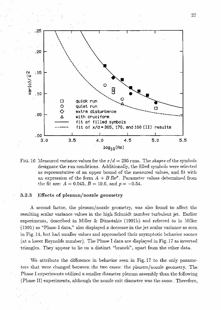
3.2.2 Effects of initial conditioils

It became apparent, during the course of the experiments discussed above, that something was influencing the behavior of the scalar variance. The cause was determined to be the fluid disturbance levels in both the jet plenum and beneath the nozzle exit. Additional runs were conducted specifically to address this issue.

One type of run made was termed a "quick run," in which the jet plenum was filled rapidly and the run started within a minute. Eliminating the usual half-hour period wait for the plenum fluid to settle resulted in a substantially higher level of fluid

motion, or disturbances, within the plenum during the run. A cruciform originally inside the plenum to damp such fluid disturbances was removed, except for one comparison run. Along with the "quick runs," other "quiet runs" were made in which the plenum fluid was left to settle for over half an hour, allowing the fluid

disturbances to decay. Finally, one "quiet run" was made in which the tank fluid immediately beneath the nozzle was given a vigorous stir with a hand, just before initiating the run. This is the "extra disturbance" run shown in Fig. 16, along with the other results.

It can be seen in Fig. 16 that, within some scatter of the results, the quick

runs have higher variance values than their corresponding quiet runs. The extra disturbance case also has a higher variance, while the run with the cruciform in place has a low variance which agrees well with a fit (dashed line) to the data previously displayed in Fig. 14. These quantitative measures of the effect of qualitatively different disturbance levels lead us to conclude that the jet variance increases with increasing disturbance level, both in the plenum and in the vicinity of the nozzle exit.

This is a somewhat surprising finding. It says that adding perturbations (in the form of disturbances) to the jet conditions causes the variance to increase, i. e.,

making the jet less well mixed. It raises the possibility that the natural, undisturbed

turbulent jet may provide the most "efficient" mixing. These results are for the liquid-phase (high Schmidt number) jet, and should be viewed in light of the earlier discussion of Sc effects. At this point, the corresponding gas-phase behavior has not been examined.

extra disturbance with cruciform fit of filled symbols

------ fit of x/d=305, 170, and100 (11) results

FIG. 16 Measured variance values for the xld = 295 runs. The shapes of the symbols designate the run conditions. Additionally, the filled symbols were selected as representative of an upper bound of the measured values, and fit with an expression of the form A + B Rep. Parameter values determined from the fit are: A = 0.045, B = 19.6, and p = -0.54.

3.2.3 Effects of plenuim/i~ozzle geoinetry

A second factor, the plenum/nozzle geometry, was also found to affect the resulting scalar variance values in the high Schmidt number turbulent jet. Earlier experiments, described in Miller & Dimotakis (1991b) and referred to in Miller (1991) as "Phase I data," also displa,yed a decrease in the jet scalar variance as seen in Fig. 14, but had smaller values and approached their asymptotic behavior sooner (at a lower Reynolds number). The Phase I data are displayed in Fig. 17 as inverted triangles. They appear to lie on a distinct "brancltl", apart from the other data.

We attribute the difference in behavior seen in Fig. 17 to the only parameters that were changed between the two cases: the pleilum/nozzle geometry. The Phase I experiments utilized a smaller diameter plenum assembly than the following (Phase 11) experiments, alt hougltl the nozzle exit diameter was the same. Therefore,

FIG. 17 Measured variance values for three major types of runs. The inverted triangles represent a different plenum/nozzle geometry. The squares are the data displayed in Fig. 16. The other symbols are the data shown in Fig. 14.

28

the contraction ratios were quite different, with Phasc I bcing smaller. In addition,

the details of the nozzle geometries differed between the two cases. The Phase I nozzle consisted of a smooth radius at the inlet and a short length of 0.254cm

( 0 . in.) I.D. tubing extending 1.8 cm (0.7 in.) beyond the plenum endplate. The tubing extension was tapered on the outside to provide a thin edge at the nozzle

exit. The Phase I1 nozzle consisted of a circular contour leading to the exit plane of the nozzle plate, with a - 3' converging angle at the exit. With no extension tube, the nozzle exit was flush with the surface of the lucite nozzle plate. Photographs of the plenum/nozzle assemblies ma37 be found in XGller (1991).

- I I I

-

0

The conclusion from these results is that the jet plenum/nozzle geometry affects the mixing occurring in these turbulent jets, as demonstrated by the changes in the

jet scalar variance. At this time, we have not isolated which particular aspects of the differences between the geometries were responsible for this behavior. However,

considering the above discussion of the influence of disturbances, both the change in

I Symbol x/d

v 100 (I) A I00 (111 - 0 170

295 0 305

- 0 -

V v

- -

I7

- 8* 4 -

I I I I

contraction ratios and the variations in the nozzles are consistent with that effect. The contraction ratio serves to amplify disturbances in the plenum fluid as it passes into the nozzle. Therefore, it might be expected that a larger contraction ratio would exhibit a larger variance, which was indeed the case.

The small extension on the Phase I nozzle, in contrast to the flush-mounted

hole of the Phase I1 nozzle, permitted a different (entrained) flow in the vicinity

of the nozzle exit. Such a flow could be more stable to small disturbances in the

vicinity of the nozzle exit. Recalling that introducing a disturbance beneath the

nozzle exit increased the variance (Fig. 16), it is likely that the Phase I nozzle is less sensitive to disturbances, and, therefore, yields a lower variance. This is also

consistent with the observed behavior.

3.3 Joint Caltech-Saadia Natioual Laboratories modeling effort

As has been described in previous reports and papers, the Two-Stage La-

grangian model, under further development in collaboration with Sandia, has cor-

rectly predicted the influence of the several parameters that control combustion generated NO,. The absolute level of the predicted emission index, however, has been too high by as much as an order of magnitude. The source of the error has

now been identified.

The model, is in essence, a description of the nature and rate of molecular

mixing, with the rate determined from scaling arguments and constants taken from

experiment. In the past, the mixing rate, because of the lack of other data, was inferred from the dependence of the flame length on the stoicluometric ratio. Fixing the scaling law constants by this procedure obviously leads to the correct dependence of the flame length on the various parameters, but since this length is determined

by the last element of nozzle fluid, to reach the stoicl~ometric ratio, the absolute value of the mixing rate so determined is mucll too low. Since the NO, emission index depends critically upon residence time which in turn depends inversely on the

mixing rate, it is now clear that a low rate yields too high an index.

What is instead the slowest rate (which determines the flame length) is a mean

rate. For a cold jet, the data from Dowling & Dimotalcis (1990) provide the neces-

sary information. For reacting jets, the temperature profiles measured by Becker & Yamazalci (1978), combined with an energy conservation analysis, yield the required

rate.

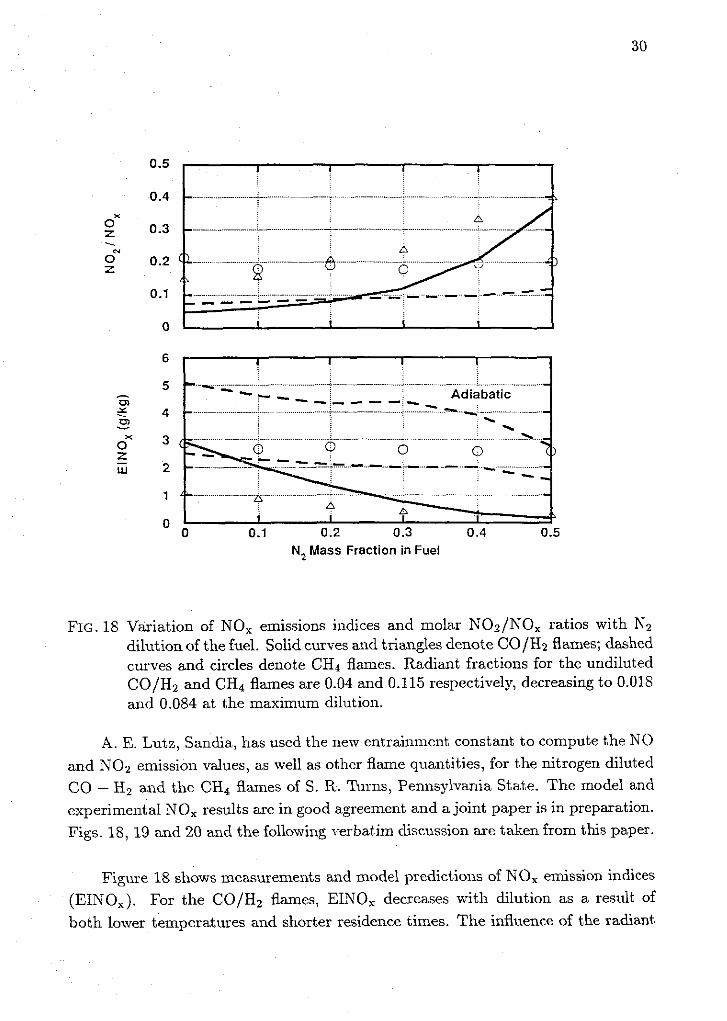
N, Mass Fraction in Fuel

FIG. 18 Variation of NO, emissions indices and molar NOz/NO, ratios with Nz dilution of the fuel. Solid curves and triangles denote CO/H2 flames; dashed curves and circles denote CHI flames. Radiant fractions for the undiluted CO/H2 and CH4 flames are 0.04 and 0.115 respectively, decreasing to 0.01s and 0.084 at the maximum dilution.

A. E. Lutz, Sandia, has used the new entrainment constant to compute the NO

and NOz emission values, as well as other flame quantities, for the nitrogen diluted CO - H2 and the CH4 flames of S. R. Turns, Pennsylvania State. The model and experimental NO, results are in good agreement and a joint paper is in preparation.

Figs. 18, 19 and 20 and the following 1-erbatim discussion are taken from this paper.

Figure 18 shows measurements and model predictions of NO, emission indices (EINO,). For the CO/H2 flames, EINO, decreases dilution as a result of

both lower temperatures and shorter residence times. The influence of the radiant

0 20 40 60 X I D

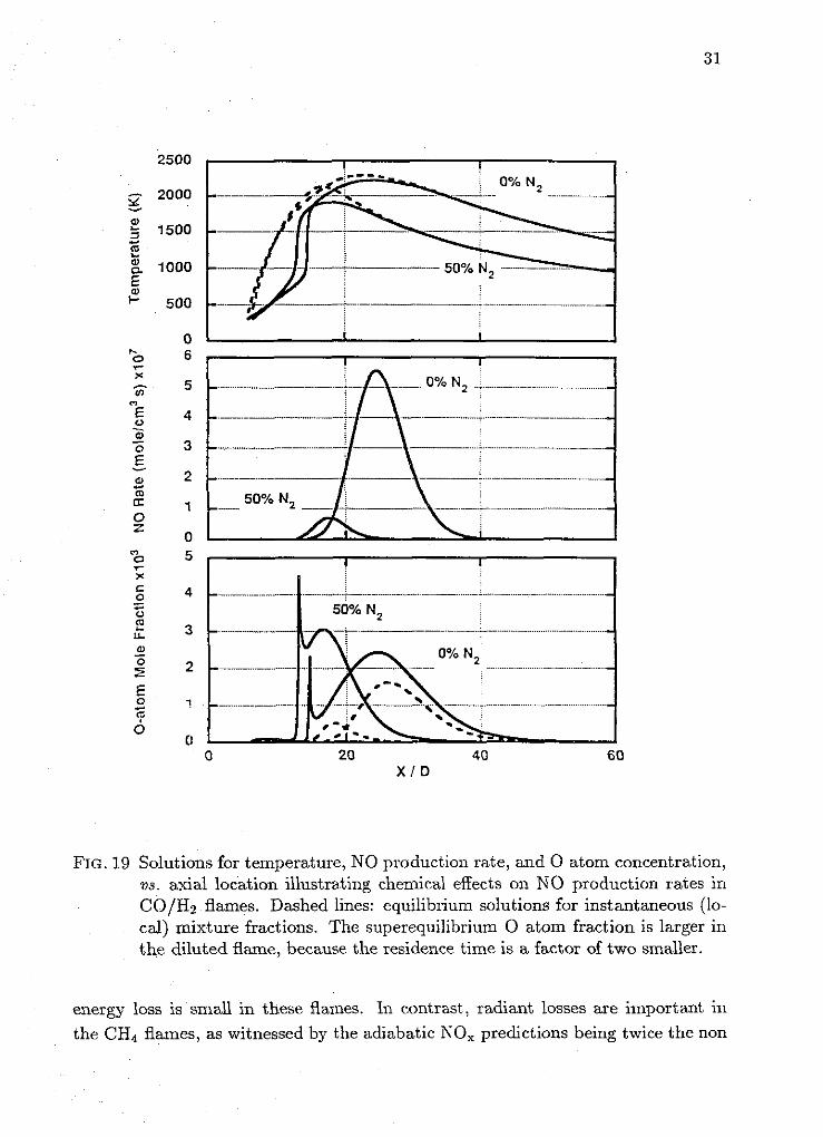
FIG. 19 Solutions for temperature, NO production rate, and 0 atom concentration, us. axial location illustrating chemical effects on NO production rates in CO/H2 flames. Dashed lines: equiliblium solutions for instantaneous (local) mixture fractions. The superequilibrium 0 atom fraction is larger in the diluted flame, because the residence time is a factor of two smaller.

energy loss is small in these flames. In contrast, radiant losses are important in

the CH4 flames, as witnessed by the adiabatic KO, predictions being twice the non

0 20 40 60 80 100 XID

FIG. 20 Solutions for the temperature, NO, emission index, and integrated Nz production vs. axial location in the undiluted CH4 flame. Solid curves: homogeneous reactor. Dashed curves: flame-sheet reactor. The integral is weighted by the relative mass in the reactors, by ~(~i~/~Ti)(m;/rn)dx. w is the mass of NzO produced per unit volume in the itheactor. ii is the average velocity. The reactions are: Thermal, Nz + 0 + NO + N; prompt, N2 + CH -+ HCN + N; and the NzO route, IT2 + 0 + M -+ NzO + M minus NzO + H + Nz + OH.

adiabatic values. Remarkably, the CH4 emission indices decrease only slightly with dilution, because, as noted above, the opposing effects of dilution leave the flame

temperature nearly constant.

Analysis of the chemical rate processes leading to NO production shows that

the thermal (Zeldovich) mechanism is the only significant route for NO formation

in the CO/H2 flames. The rate-determining step in this mechanism is the reaction

Since the Nz mole fraction remains nearly constant, NO production in these flames

depends on two factors: the 0 atom concentration history and the temperature history.

Figure 19 illustrates the degree to wluch predicted 0 atom concentrations are

in excess of their equilibrium values (dashed curves). The 0 atom superequilibrium ratio is greater for the Nz diluted flame ([0]/[0],,, = 6.2 vs. 1.5), since residence time in this flame is less than half in the undiluted flame (1.7ms us. 4ms). The

spikes in the kinetic 0 atom conccntrations occur when the cold mixture in the homogeneous reactor is ignited by the hot stoichiometric mixture in the flame sheet reactor.

More important to NO production is the departure from equilibrium of the flame temperature. Peak temperatures are suppressed approximately 50IC and

250K for the undiluted and 50%-Nz flames, respectively (Fig. 19). The temperature during NO production is lower in the diluted flame, so the NO production

rate is slower despite the higher 0 atom concentrations. The temperature effect overwhelms the concentration effect, because the thermal NO reaction has a large

activation energy (close to 75kcal/gmole), as noted by Correa e t al., (1984).

I11 the CH4 flames, the NO formation chemistry is complicated by the contri-

bution of the prompt mechanism, as initiated by the reaction Nz + CH -+ HCN + N. The free N atom easily forms NO by collision with either 5 2 or OH. The HCN

radical can lead to either production or coilsumption of NO. The prompt initiation

step breaks apart 30% of the Nz that is consumed, compared to 60% via the thermal

mechanism (Table I and Fig. 20). The renlaining N2 consumption (10%) occurs via the N 2 0 route,

N 2 + O + h 4 -+ N 0 2 + M ,

which has a rate comparable to the thermal initiation step,

TABLE I Contributions of various kinetic mechanisms

to total NO production in undiluted CH4 flames

Nz consumption (% of total in both reactors):

Path Honlogeneous

Thermal 15 NzO route 4 Prompt 0

NO production (% of total in both reactors):

Path Hoinogeneous Thermal(a) 2 1 Prompt (b) 0 NO2 conversion -12 HNO loop -3

(a)Nz + 0 --t NO + N; N + O z + N O + O ; N + O H + N O + H

(b)CN + 0 -+ C + NO; HCN + 0 --t CH + NO; HCNO + H -+ CH2 + NO;

HCNO + CO -+ HCCO + NO;

COz + N --t NO + CO; NCO + 0 --t NO + CO

except that most of the NzO returns to N2 by collision with H atoms. Of the total

Nz consumed in the simulation, 80% occurs in the flame-sheet reactor, which is not

surprising, because the mixture here is hot during the whole flame length. Similarly, 94% of the total NO production comes in the flame-sheet reactor. The contribution of the honlogeneous reactor occuss via the thermal mechanism when the reactor

ignites at x/d = 80 (Fig. 20).

We exercised the model u~itliout the prompt reactions included in the mecha-

nism and found that the computed EINO, was 30% lower than predicted by the

full mechanism. While this agrees with the N2 consumption associated with the prompt initiation step above, we caution that superposition does not strictly apply to the nonlinear solution.

The evolution of the NO, emission index in the simulation (Fig. 20) indicates

that prior to the ignition of the homogeneous reactor, NO, produced in the flame-

sheet is transported to the honlogeneous reactor. When the buoyant switch accel-

erates the entrainment of cold surroundings at ic/d = 70, a period of transient NO conversion to HNO occurs in the flame-sheet (dashed curve) via a three-body reac-

tion with H atoms. Shortly thereafter, when the homogei~eous reactor ignites, NO

production proceeds again, until the fuel is exhausted and the temperature begins to decay. The final emission level comes as a result of the fluid exchange between reactors as they continue to entrain cold air.

Next we examine the NOz fraction of the total NO,. The NO2 fraction increases as the CO/H2 flames are increasingly diluted, while the NO2 fractions are unaffected by dilution in the CH4 flame (Fig. 19). The model predictions and experiments are in excellent agreement, especially considering the small absolute quantities of NO2

produced. Although the NO2 fractions increase in the CO/H2 flames, NOz emission indices (EIN02) actually decrease with Nz dilution (0.137 - 0.06lg/kg predicted

for 0.50% N2). The model predicts that the NO2 is formed after NO formation is complete, well downstream of the maximuin temperature. It is also interesting to note that the peak NO2 production occurs in all of the flames in the temperature range of 1100 - 1400 I<.

In conclusion, predictions from a turbulent jet flame model that employs a relatively simple model of fluid mixing but detailed chemical kinetics were compared

with experimental measurements from Nz-diluted CO/H2 and CH4 flames. The model predictions of NO and NO2 emission indices are in good qualitative and reasonable quantitative agreement with nleasurements from both flames. Inclusion

of the radiant heat losses is necessary to predict NO, levels and trends with Nz dilution from the CH4 flames. The thermal mechanism is the only significant rout

for NO formation in the homogeneous reactor model of CO/H2 flames. It is also the dominant route in the CH4 flames, except for a 30% contribution of the prompt

mechanism, which appear in the flame-sheet reactor only.

The different channels of NO, formation reasonably well predicted by a detailed

chemical kinetics model contribute to a better understanding and controlling NO,

emissions from combustion sources. The model is now in good agreement with experimental results, after the mixing rate was determined to be too low, originally.

4. Analytical a n d con~pu ta t iona l effort

A new approach for computing inultidimensional flows of an inviscid gas has

been developed as part of our on-going computational effort. It may be considered an extension of the method of cllaracteristics to multidimensional, unsteady gas

dynamics.

The idea is to use the ltnowledge of the one-dimensional characteristic problem

for gasdynamics to compute genuinely multidimensioilal flows in a mathematically consistent way. A family of spacetime manifolds is found on which an "equivalent"

1-D problem holds. These manifolds are referred to as Riemann Invariant Manifolds

and play the role that the characteristic manifolds play in the method of character-

istics for 1-D unsteady or 2-D steady gas dynainics. Their geometry depends on the local spatial gradients of the flow and they provide locally a convenient system of

coordinate surfaces for spacetime. In the case of zero entropy gradients, functions analogous to the Riemann invariants of 1-D gasdynainics can be introduced. These generalized Riemann Invariants are constant on the Riemann Invariant Manifolds.

The equations of motion are integrable on these manifolds and the problem of computing the solution becomes that of determining the geometry of these manifolds

locally in spacetime. This theory allows one to 100li at such flows in a very useful

way, reminiscent of the method of characteristics. A whole family of numerical schemes can be devised using these ideas.

The progress made in recent years in the development of numerical schemes for computing such flows is based on the various higher order extensions of the

original Godunov (1959) scheme. These schemes allow high order accuracy without

spurious oscillations near the flow discontinuities. The main idea of the Godunov scheme and its extensions is to use the kno~vledge from the theory of characteristics,

locally in each con~putational cell, to compute the various flux terms. By doing this, the local characteristic wave patterns are accounted for, accurately. Since discontinuities are likely to be present, the characteristic problem is generalized to allow for their presence. This constitutes the well known Riemann problem. Two

arbitrary constant states, separated by a discontinuity in space, are given as the

initial condition. The solution to the Riemann problem is used as the building block for numerical methods of this type. It provides the information needed to compute

the fluxes at the interfaces of the computational cells.

Although the application of this idea is straightforward for the one-dimensional case, the extension to multidimensional flows is not. Practically, these schemes are

extended to more dimensions by treating the additional spatial dimensions separately. The computation is not truly multidimensional, but rather a number of separate one-dimensional computations in each spatial direction. Even schemes that appear to be multidimensional (unsplit), actually use the local directions of

the grid to set up and solve a 1-D Rieinann problem, thus taking advantage of the

1-D results. The only real effort to create a inultidimensional scheme are those by Roe (1986), Hirsch & Lacor (1989), and Deconick e t al. (1986).

We have used the Riemann Invariant Manifold theory to develop a novel

scheme. This scheme is a standard high-order shocli-capturing Godunov scheme which has been modified to take into account the multidinlensional character of the

flow in a mathematically consistent way. No flus-splitting or other multidimensional

"fixes", that are usually employed, are needed. This n~ultidimensional correction can be directly extended to three-dimensional flows. l i e are currently testing this

scheme on a variety of test problems.

A first paper, documenting our earlier, 1-D unsteady gasdynamic flow simulation method, has been accepted for publication (Lappas et al. 1992).

5. Diaglrostics and instrunlelitation development

Our diagnostic and instrumentation development is proceeding very well. A new instrument to measure the turbulent structure(s) convection velocity was pre-

viously mentioned in Sec. 2.4, and will not be discussed further here.

As part of a major effort, we have developed the capability to acquire data at very high rates, beyond those achievable with conlmercial devices. This will permit

us to acquire sequences of high resolution images, using CCD cameras. Additionally, we are proceeding with the design of electronics to support a custom CCD array, designed in collaboration with JPL, which has been dubbed the "MACH CCD." The

MACH CCD will permit us to record two high-resolution images within a fraction

of a microsecond of each other. \ire will then be able to image supersonic flows, and,

utilizing image correlation velocimetry techniques, determine the two-dimensional velocity field in the plane of the images.

5.1 High-speed data acquisitioli

We have completed the &st two A/D converter boards for high speed and high resolution image acquisition. The first board has two 12 bit 15 megahertz A/D converters and can digitize two analog inputs at 15 MHz or one input at 30 MHz. The second board has two 12 bit 20 megahertz AID converters and can digitize

two inputs a t 20 MHz or one input at 40 MHz. Both boards have 32 megabytes of

local buffer memory and plug into a standard VXI backplane. A VMEbus computer

running the 0s-9 real time operating system controls the A/D converters through a VME to VXI bus converter. The 0s -9 system can transfer the acquired images

to the VAXcluster through the Ethernet.

The A/D subsystem has been used with a Hitachi high resolution RGB camera. The camera has three CCD's (one per color) with a resolution of 560H by 480V pixels. A phase locked loop has been built for the Hitachi camera to reconstruct the pixel clock and synchronize the 4 / D converter boards. We can digitize up to 56 consecutive frames when digitizing 2 of the three colors or up to 28 consecutive

frames digitizing all 3 colors.

We have also used a high resolution black and white camera manufactured by Texas Instruments (resolution of 1134H by 480V pixels). This camera has a pixel clock output, so a small board was constructed to buffer the pixel clock, horizontal

sync, and vertical sync for the A/D converter boards. One A/D converter board can

digitize up to 28 consecutive frames (this can be extended to 56 frames by chaining

a second board after the first).

Additionally, we are designing a controller board that will be able to control

the MACH dual image CCD camera being built by JPL. The controller board will

have two microsequencers. The first (pixel) microsequencer will generate the com- plex waveforms needed by the LII.4CH CCD camera and control the A/D converter

boards. The pixel microsequencer can be progranlmed to digitize a subset of the

image (region of interest) in order to conserve memory. The second (real time)

microsequencer is used to generate the timing waveforms for the YAG lasers, the camera shutter, and other laboratory devices. Both microsequencers can be trig-

gered from an external control signal or from the other microsequencer.

For instance, the real time microsequencer can wait for an external trigger signal

(e.g. the start of a run), then fire the first Y.4G laser, tell the pixel microsequencer to store the first image, then fire the second YAG laser, and finally tell the pixel microsequencer to start digitizing the two images. The MACH CCD should be able

to acquire two images as short as 200 nanosecollds apart.

5.2 Image cor.relatioil velociilletry

We are developing the capability to use the correlation of two scalar images

for the purpose of motion detection. In particular, .cx-e can map the deformation of a flow field over time. Quantities like the velocity, vorticity, and strain rate are

estimated directly from a pair of scalar images. Initial investigations designed to tune tlus process have examined the flow past a circular cylinder.

To measure the movement of a scalar image over time, consider two images or

scalar fields (e.g., dye, temperature, or density), spaced in time. It is clear that there is a mapping taking the first image to the second. One such mapping is

simply the motion of the fluid together with the equations of motion of the scalar.

Integrating the equation of motion of a scalar, over time, we may write:

where 5 (x) is some (vector) coordinate transformation mapping the image taken at

time to, It, (x), to the image at time t l , It, (x). The unknown, and highly nonlinear vector transformation E(x), is then calculated by solving Eq. 12. A more reliable

method is to minimize Eq. 12 over some volume V, e.g., in a least squares sense,

2

min / [I,, (5 (x)) - I t ) - D 1; v21 ( ~ ( t ) ) dt ] dx 50 v

(13)

Now consider that [(x) is just a displacenlent of some point x to another ((x). Since 5 (x) is a complicated nonlinear functioil we linearize (locally expand) in a

neighborhood N about a point x, so,

Clearly 5 (x) is the displacement (velocity) of the center of N , and (x - x) . VE (k) is the local deformation (rotation, strain, dilatation, etc.), that N experienced when

moving from x to ((x).

Note that the state of the art in image velocimetry does no better than the

first order displacement, <(x), of Ar. Using Eqns. 13 and 14 over a neighborhood

N yields,

min / ~ t , ( 5 ( 2 ) + ( x - x ) . V € ( 2 ) + . . .)- It,,(x)- t(x),v€(x),... n/

Note that there is little justification in going beyond the second order term in Eq. 15. This is because of the rapid increase in the number of paranleters that occurs when going to higher order in the minimization. Trying to fit too many parameters would be time-consuming, and, in the presence of noise, meaningless.

Our experience suggests that a second order expansion of the displacement field will yield better velocity estimates than results using a traditional first or-

der approximation. Keeping the second order terms in the minimization (Eq. 15) increases the reliability of the first order term, particularly in regions where the flow contains large velocity gradients or rotational motions. In addition, the local vorticity, strain, and divergence can be determined directly from the minimization

parameters, obviating the large errors inherent in using only the first order estimate of the displacement and the11 differentiating to obtain these higher order derivatives

of the flow field.

The high-speed data acquisition is part of the work by D. Lang, and the scalar correlation velocimetry is being carried out by P. Tokumaru, both in collaboration with P. Dimotakis.

6. Personnel

In addition to the Principal Investigators:

P. E. Dimotakis: Professor, Aeronautics & -4pplied Physics;

J. E. Broadwell: Senior Scientist, -4eronautics;

A. Leonard: Professor, Aeronautics;

other personnel who have participated directly in the effort during the current reporting period are listed below (all are in the Aeronautics option):

C. L. Bond: Graduate Research Assistant;

H. J. Catrakis: Graduate Research Assistant;

E. Dahl: Member of the Technical Staff;

D. C. Fourguette: Post-doctoral Research Fellow;

R. J. Gilbrech: Graduate Research .4ssistant;

J. L. Hall: Graduate Research Assistant; *

D. B. Lang: Staff Engineer;

T. Lappas: Graduate Research Assistant;

P. L. Miller: Post-Doctoral Research Fellow;

H. Rosemann: Post-doctoral Research Fellow; **

P. T. Tokumaru: Post-doctoral Research Fellow.

fl Ph.D., June 1991; presently working for KASA's Stennis Space Center, Mississippi.

* Ph.D., June 1991.

** Appointment ended, June 1991; presently working for the DLR, Gottingen, Germany.

7. References

Bibligraphical references denoted by a bullet (e) in this list below represent

publications of work under the sponsorship of this Grant that have appeared during

the present reporting period.

BATCHELOR, G. I<. 1959 L'Small-scale variation of convected quantities like temperature in turbulent fluid. Part 1. General discussion and the case of small con-

ductivity," J. Fluid Alech. 5, 113-133.

BECKER, H. A. & \'AMAZAKI, S. 1978 "Entrainment, Momentum and Tempera-

ture in Vertical Free Turbulent Difusion Flames," Comb. and Flame 33, 123-149.

CHEN, C. J . & RODI, W. 1980 Vertical Turbulent Buoyant Jets. A Review of Experimental Data (Pergammon Press, Odord).

CHINZEI, N., MASUA, G., I<OMURO, T. MURAICAIII, A. & I ~ U D O U , I<. 1986 '6 Spreading of two-stream supersonic turbulent mixing layers," Phys. Fluids 29,

1345-1347.

CLEMENS, N. T . & MUNGAL, M. G. 1990 "Two- and Tliree-Dimensional Effects in the Supersonic Mixing Layer," 26th AIA24/SAE/ASA!fE/ASEE Joint Propulsion Conference, Paper 90-1978.

CORREA, S.M., DRAKE, M.C., PITZ, R.W. & SIIYY, W. 1984 "Prediction and Measurement of a Non-Equilibrium Turbulent Diffusion Flame," 2oth Symposium (Int) on Combustion, p.337, The Combustion Institute.

DECONINCK, H., HIRSCH, C. & PEUTEMAN, J . 1986 "Characteristic Decom- position Methods for the Multidin~ensional Euler Equations," loth International Conference on Numerical Methods in Fluid Dynamics (Beijing, June 1986).

e DIMOTAKIS, P. E. 1991 "Fractals, dimensional analysis and similarity, and turbulence," Nonlinear Sci. Today #2/91, pp. 1, 27-31 (Appendix C, this report).

l DIMOTAKIS, P. E. 1991 "Turbulent Free Shear Layer Mixing and Combustion,"

High Speed Flight Propulsion Systems, in Progress in Astronautics and Aeronautics

137, Ch. 5, 265-340.

DIMOTAICIS, P . E. & MILLER, P . L. 1990 "Some consequences of the boundedness of scalar fluctuations," Phys. Fluids A 2(11), 1919-1970.

DOWLING, D. R. 1988 Mixing in Gas Phase Turbulent Jets, Ph.D. thesis, Califor- nia Institute of Technology.

DOWLING, D. R. & DIMOTAKIS, P . E . 1990 "Sinlilarity of the concentration field of gas-phase turbulent jets," J. Fluid Mech. 218, 109-141.

GILBRECH, R. J. 1991 An Experimental Investigation of Chemically-Reacting,

Gas-Phase Turbulent Jets, Ph.D. thesis, California Institute of Technology.

GILBRECH, R. J. & DIMOTAICIS, P . E. 1992 "Product Formation in Chemically-

Reacting Turbulent Jets," AIAA 3oth Aerospace Sciences hfeeting, AIAA Paper 92-0581 (Appendix B, this report).

GODUNOV, S. I<. 1959 "A Finite Difference Method for the Numerical Computa- tion of Discontinuous Solutions of the Equations of Fluid Dynamics," Mat. Sb. 47,

271-306.

HALL, J . L. 1991 An Experimental Investigation of Structure, Mixing and Com- bustion in Compressible Turbulent Shear Layers, Ph.D. thesis, California Institute

of Technology.

HIRSCH, C. & LACOR, C. 1989 "Upwind Algorithnls Based on a Diagonalization

of the Multidimensional Euler Equations," AI4.4 Paper No. 89-1958.

KEE, R. J. , MILLER, J . A. & JEFFERSON, T. H. 1980 "CHEMIiIN: A General Purpose, Problem-independent, Transportable, Fortra.11 Chemical Iiinetics Code

Package," SANDIA Report SANDSO-8003.

a LAPPAS, T., LEONARD, A. & DIMOTAKIS, P . E. 1992 "An Adaptive Lagrangian

Method for Computing 1-D Reacting and Non-Reacting Flows," J. Comp. Phys. (to appear).

o MILLER, P . L. 1991 Mixingin High Schmidt Number Turbulent Jets, Ph.D. thesis, California Institute of Technology.

MILLER, P . L. & DIMOTAICIS, P . E. 1991a "Stochastic geometric properties of scalar interfaces in turbulent jets," Phys. Fluids A 3(1), 168-177.

MILLER, P. L. & DIMOTAI<IS, P. E. 1991b "Reynolds number dependence of scalar fluctuations in a high Schmidt ilumber turbulent jet," Phys. Fluids A 3(5),

1156-1163 (Appendix A, this report).

MILLER, P. L. & DIMOTAKIS, P. E. 1992 "Measuren~ents of scalar power spectra

in high Schmidt number turbulent jets," Pl~ys. Fluids A (submitted).

PAPAMOSCHOU, D. 1989 "Acoustic Paths in Con~pressible Shear Layers," Bull. Am. Phys. Soc. 34(10), 2252.

PAPAMOSCHOU, D. & ROSHKO, A. 1988 "The Compressible Turbulent Shear

Layer: An Experimental Study," J. Fluid Atech. 197, 453-477.

ROE, P. L. 1986 "Discrete Models for the Numerical Analysis of Time-Dependent Multidimensional Gas Dynamics," J. Comp. P l~ys . 63, 458-476.

WHITE, F. M. 1974 Viscous Fluid Flow (McGran-Hill, New York).

Appendix A

MILLER, P. L. & DIMOTAKIS, P. E. 1991 "Reynolds number dependence of scalar fluctuations in a high Schmidt number turbulent jet," Phys. Fluids A 3(5), 1156-

1163.

Reynolds number dependence of scalar fluctuations in a high Schmidt number turbulent jet

Paul L. Miller and Paul E. Dlrnotak~s Graduate AeronauncalLaborator~es. Callfornra Instrtute of Technology, Pasadena, Calr/ornm 91125

(Received 28 August 1990; accepted 9 January 1991 )

The scalar r m s fluctuations in a turbulent jet were investigated experimentally, using high- resolution, laser-induced fluorescence techniques. The experiments were conducted in a high Schmidt number fluid (water), on the jet centerline, over a jet Reynolds number range of 3000GReG24 000. It was found that the normalized scalar rms fluctuations c'/ 7 decrease with increasing flow Reynolds number, at least for the range of Reynolds numbers investigated. Since c'/ 7 is a measure of the inhomogeneity of the scalar field, this implies that high Schmidt number turbulent jets become more homogeneous, or better mixed, with increasing Re. These findings need to be assessed in the context of the documented Reynolds number independence of flame length for Re > 3000 or 6500.

I. INTRODUCTION

The correct description of the probability density function (pdf) of the fluctuations of a conserved passive scalar in turbulent flow has been a matter of theoretical and engineer- ing interest for some time. Knowing the pdf of the conserved scalar allows the computation of the amount of chemical product that would be formed in a chemical reaction in which the scalar is transported as a passive quantity.'

Experimental evidence and theoretical arguments in the last few years suggest that the turbulent mixing process is sensitive to the value of the molecular diffusion coefficients, even at Reynolds numbers typically regarded as high. We recognize that this remains a controversial proposal, at this writing, especially in the case of turbulent jet mixing.' We note, in particular, that accepting it would imply that the conserved scalar pdf, as well as other statistics of the mixing process, should beexpected to be functions of the flow Reyn- olds number Re = U6/v, where U is the local flow velocity, 6 is the local extent of the turbulent flow and v denotes the (molecular) kinematic viscosity, and the Schmidt number Sc = v / g , where 9 is the scalar species (molecular) diffusivity. There is no consensus at this time as to how such effects should be described, let alone predicted, with the associated nonlinear dynamics essentially involving terms in the equations of motion with factors that vanish, multiplied by factors that become unbounded in the limit of Re- W , or Sc-oc.

Nevertheless, the qualitative dependence on Sc might be argued on simple grounds, namely, that decreasing the species diffusivity, i.e., increasing the Schmidt number, keeping all other flow and fluid quantities fixed, can only decrease the rate of (molecular) mixing and the amount of mixed fluid. This is corroborated by a comparison of the results of experiments in gas phase shear layersZ (Sc- 1 ) versus those in liquid phase shear layers4 (Sc - 10') at comparable Reyn- olds numbers.

An a priori argument for the dependence on Reynolds number is not as straightforward. Reliable experimental

data at large Reynolds numbers are difficult to obtain. Ex- periments at high Reynolds numbers must rely on chemically reacting flows to infer the degree of molecular mixing. In the case of gas phase shear layers, the experimental evidence from a single experiment is that the amount of mixing decreases as the Reynolds number increases, albeit ~ l o w l y . ~ The evidence shows a Reynolds number dependence in liquid phase shear layers that appears to be weaker, but this conclusion is based on scanter data.4

In turbulent jets, the behavior is even less clear. Experi- mental "flame length" data in liquid jets,' as well as other liquid and gas phase turbulent jet flame length data reviewed in Fig. 1 of Dahm and Dimotakis,' suggest that this quantity may well be independent ofboth Schmidt number and Reyn- olds number, at least for Reynolds numbers greater than about 3 X lo', or so, as had been reported in the earlier Wed- dell"(see also Hottel, Ref. 9 ) findings. The scatter in these data is large enough, however, to have masked a weak dependence on Schmidt number or Reynolds number, not to speak of thelikely contamination of the results by buoyancy effects in the case of high heat release, gas phasejet flames. As a case in point, the results of Kristmanson and Danckwerts"' suggest that Reynolds number independence of the flame length in a liquid jet does not occur until a Re greater than 6500, or SO.

More recently, direct measurements of the jet fluid concentration pdf in gas phase turbulent jets by Dowling and Dimotakis" suggest a Reynolds number independence, at least in the Reynolds number range from 5.OX 10' to 4.0X 10'. These authors also compare their estimates of the jet fluid concentration pdf on the jet axis with those measured b; other investigators,"-'" for Schmidt (Prandtl) numbers ranging from 0.7 to 10' and Reynolds numbers ranging from 5 X 10" to 5.2 x lo4 (Dowling and Dimota- kis," Fig. 28). While the reported pdf's may not collapse particularly well, it is difficult to assess whether the differences are attributable to Schmidt number or Reynolds number effects, or to experimental difficulties.

Our own investigations of the behavior of the turbulent

1156 Phys Flulds A 3 (5). May 1991 0899-821 3191 1051 156-08502 00 G 1991 Amer~can lnstltute of Physlcs 1156

jet fluid concentrat~on fluctuatlons were undertaken as part of a larger effort to address the role of Reynolds number as a parameter in the dynamics of turbulent jet mlxing. The experiments reported here were performed in liquld phase turbulent jets (Sc- lo3)), in a Reynolds number range from 3.OX 10' to 2.4X lo'. Our measurements permitted direct estimates of the pdf, m s , as well as the spectrum of the conserved scalar fluctuatlons to be computed.

11. APPARATUS AND PROCEDURE

While the experimental setup has been documented previ~usly,~." the following short description is included for completeness. The experiments were carried out utilizing the facility shown in Fig. 1. A large rectangular water tank, about 1 m square and 2 mhigh, acted as the (discharge) reservoir. Large windows on all sides of the tank provided optical access. To establish the flow, thejet plenum was filled with water tagged by a fluorescent laser dye (sodium fluorescein) and air was sonically metered to drive the jet fluid at constant velocity through a 2.54 mm (0.1 in.) diam nozzle at the base of the plenum. The beam from an argon-

ion laser was passed through appropriate optics and aligned radially through the centerline of the jet. A beam stop prevented reflections from the opposite window. For these measurements, the laser beam optics were designed to generate a small Gaussian waist at the focus. A low laser power of 1.0 W was used to avoid heating of the dyed fluid in the very small focal volume and to prevent saturation. The plenum dye concentration was kept less than 1 0 ' M. Consequent- ly, the much lower concentrations at the measuring station did not significantly attenuate or steer the beam.

A low f # lens was used to collect light from a short segment centered at the waist of the focused laser beam (on the jet centerline, at x / d = 100) onto a photomultiplier tube, effectively yielding single-point concentration values versus time. An optical low-pass filter eliminated hack- ground laser light, transmitting only the frequency-shifted fluorescence. A slit spatial filter defined the length of the laser line segment sampled. The slit width was chosen such that the sampling volume was roughly cylindrical, about 80 p m in diameter and less than 50pm in length. The use of the slit rather than a pinhole ensured that any small transverse beam movements did not alter the measurement volume. The long Rayleigh range and latitude in the depth of field

FIG 1 Expenmental apparatus

11 57 Phys Flutds A, Vol 3, No 5, May 1991 P. L. Miller and P. E. Dimotakis

minimized theeffect of motion in either of the two horizontal directions. Data acquisition was computer-controlled. The signal amplifier incorporated a three-pole Butterworth filter, with a cutoff frequency set slightly under 10 kHz. The data were sampled at 20 kHz for all the runs.

Careful consideration has been given to the reduction of noise in these measurements, especially since we wish to examine the normalized scalar rms fluctuations, c'/ ?. As described previous ly ,"~ 'be utilized Wiener filter tech- n i q u e ~ ' ~ . ~ ~ in processing the data. The issues of buoyancy and attenuation of the laser beam have been examined, and are discussed in Appendix A. We conclude that neither is a factor in these jets. Finally, an important consideration when measuring a quantity such as c'/Z is resolution, since fluctuations at scales smaller than the measuring volume are low-pass filtered. It is therefore necessary to determine that either the smallest scales of the flow are resolved or that the contribution to the fluctuations by scales smaller than the resolution is negligible. We discuss resolution concerns later in this paper.

Ill. RESULTS

For our discussions, the jet Reynolds number is defined as Re = U, ,d / v , where U,, is the jet exit velocity, d is the diameter of the jet nozzle, and vis the kinematic viscosity of the working fluids (water).

Our measurements indicate that thescalar field of a high Schmidt number turbulent jet has, in some sense, not reached an asymptotic state for Re as large as 10 000 to 20 000, or more. This is apparent in the behavior of the scalar pdf 's with varying Re. In Fig. 2, we show four sample pdf 's, spanning Reynolds numbers from 3000 to 24000. One hundred and fifty histogram bins were used to compile each pdf. Approximately 34 large-scale structure passages were captured at the lowest Re, and over 125 at the highest.

These pdf 's display a decreasing relative concentration fluctuation amplitude and imply that the jet is becoming more homogeneous in composition with increasing Re. It could be argued that this may be attributable to worsening resolution, as Re increases. It turns out, however, that the

c / c

FIG 2 Scalar pdf 'r for varytng Re (on axts, x / d = 1 W)

effect is not due to resolution difficulties, as will he addressed below.

Another manifestation of a change with Re is in the corresponding scalar power spectra (Fig. 3). Here, we plot the spectra E, ( fr, ) at the four Reynolds numbers, normalized by the estimated large-scale times,

and the local mean concentration squared, F2. The frequency axis has also been nondimensionalized by 7,. With these nor-. malizations, equal (equivalent) length scales line up on the fi, axis, regardless of Re. The large-scale passage frequencies, as independently estimated by the local centerline velocities divided by the width of the jet, are seen to he aligned at fr, = 1, corresponding to the length scale 6. So, alternatively, the f ~ , axis can he viewed as a nondimensional, in- verse length scale, which is the same for all Re. This view will be useful in the discussion below.

An important observation is that these spectra do not collapse when normalized in this fashion. The central (mid- frequency) portion of the spectra can be seen to bulge up- ward with decreasing Reynolds number. This might, perhaps, be understandable given the low Re involved and the documented reluctance of the jet spectrum to develop a constant slope region until at much higher Re. However, in addition to the shape differences, there is a discrepancy between the low-frequency levels of the spectra. If the normalization was the cause of these discrepancies, the only "free" parameter would be T*, the estimate of the large-scale time.

Two considerations help to rule out attributing the variations to the value of 7,. One is that, since 7, multiplies the frequency but divides the spectrum, changes in T, shift the normalized spectra along lines of slope - 1. This does not improve thecollapse. Thesecond point is that the ratio of the constant level region at the lowest Re to that at the highest Re is greater than 2. A variation in T,, by this amount is not admissible by the uncertainties in this quantity. Therefore, possible uncertainties in normalization cannot explain the variation in the spectra observed.

FIG. 3. Normalized scalar power spectra for vary~ng Re (on axir. x / d = 100)

1158 Phys. Fluids A, Vol. 3, No. 5, May 1931 P. L. Miller and P. E. Dirnolakis 11 58

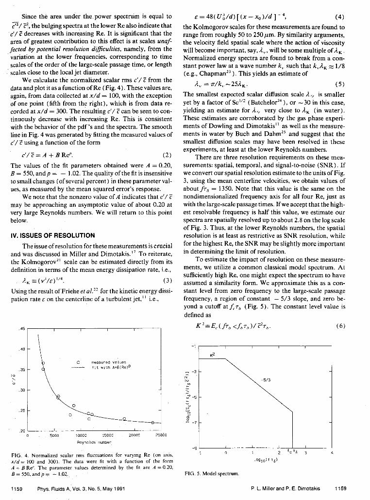
Since the area under the power spectrum is equal to

p/ T2, the bulging spectra at the lower Re also indicate that c'/ T decreases with increasing Re. It is significant that the area of greatest contribution to this effect is at scales unof- ferted by potential resolution drfficulties, namely, from the variation at the lower frequencies, corresponding to time scales of the order of the large-scale passage time, or length scales close to the local jet diameter.

We calculate the normalized scalar rms c'/ T from the data and plot it as a function of Re (Fig. 4). These values are, again, from data collected at x/d = 100, with the exception of one point (fifth from the right), which is from data recorded at x/d = 300. The resulting c'/ T can be seen to continuously decrease with increasing Re. This is consistent with the behavior of the pdf's and the spectra. The smooth line in Fig. 4 was generated by fitting the measured values of c'/ T using a function of the form

The values of the fit parameters obtained were A = 0.20, B = 550, andp = - 1.02. The quality of the fit is insensitive to small changes (of several percent) in these parameter values, as measured by the mean squared error's response.

We note that the nonzero value of A indicates that c'/ T may be approaching an asymptotic value of about 0.20 at very large Reynolds numbers. We will return to this point below.

IV. ISSUES OF RESOLUTION

The issue of resolution for these measurements is crucial and was discussed in Miller and Dimotakis." To reiterate, the Kolmogorov2' scale can be estimated directly from its definition in terms of the mean energy dissipation rate, i.e.,

1, 5 ( S / E ) " ~ . (3)

Using the result of Friehe et a/." for the kinetic energy dissipation rate E on the centerline of a turbulent jet,'' i.e.,

FIG. 4. Normalized scalar rms flucluations for varying Re (on axls. x / d = 100 and 300). The data were fit wirh a function of the form A + B Re". The parameter values determined by the f i t are A = 0.20. B = 550. and p = - 1.02.

the Kolmogorov scales for these measurements are found to range from roughly 50 to 250pm. By similarity arguments, the velocity field spatial scale where the action of viscosity will become important, say, A,., will besome multiple o f l , . Normalized energy spectra are found to break from a constant power law at a wave number k,. such that k,.A, =: 1/8 (e.g., Chapman2' 1). This yields an estimate of

A,, = rr/k%.-2SAK. ( 5 )

The smallest expected scalar diffusion scale 1 , is smaller yet by a factor of S C " ~ ( B a t ~ h e l o r ~ ~ ), or -30 in this case, yielding an estimate for A,, very close to 1, (in water). These estimates are corroborated by the gas phase experiments of Dowling and Dimotakis" as well as the measurements in water by Buch and Dahm25 and suggest that the smallest diffusion scales may have been resolved in these experiments, at least at the lower Reynolds numbers.

There are three resolution requirements on these measurements: spatial, temporal, and signal-to-noise (SNR) . If we convert our spatial resolution estimate to the units of Fig. 3, using the mean centerline velocities, we obtain values of about frA = 1350. Note that this value is the same on the nondimensionalized frequency axis for all four Re, just as with thelarge-scale passage times. If we accept that the highest resolvable frequency is half this value, we estimate our spectra are spatially resolved up to about 2.8 on the log scale of Fig. 3. Thus, at the lower Reynolds numbers, the spatial resolution is at least as restrictive as SNR resolution, while for the highest Re, the SNR may he slightly more important in determining the limit of resolution.

To estimate the impact of resolution on these measurements, we utilize a common classical model spectrum. At sufficiently high Re, one might expect the spectrum to have assumed a similarity form. We approximate this as a constant level from zero frequency to the large-scale passage frequency, a region of constant - 5/3 slope, and zero beyond a cutoff atf;.r, (Fig. 5 ) . The constant level value is defined as

K '-- E, ( fr, <f, r, )/ FZr,, . ( 6 )

FIG. 5. Model spectrum.

1159 Phys Flulds A. Vol 3, NO 5. May 1991 P. L. Miller and P. E. Dimotakis 1159

The spectrum is normalized here to the variance of the scalar fluctuations, i.e.,

which relates the spectrum directly to c'/ 7. We integrate the model spectrum

to obtain the result

cP/F=K{2+3[1 - ( f~/f;)2"])"2. (9 )

On the jet axis and at fixed x/d, this can be expressed as a function of Reynolds number by substituting forf , and f, (cf. Dowling'"), yielding

Several things are apparent from Eq. ( 10). First, it indicates that c'/ 7 would be expected to increase slightly with Reynolds number. This is opposite to the trend exhibited by our data. Also, we note that at infinite Reynolds number Eq. (10) predicts a finite value for c'/ ?of v'5 K. To evaluate this expression for our measurements, we fit the level, low-frequency, portion of our highest Re spectrum to determine K2, yielding K'z0.0078 and an asymptotic value of c'/ T=0.198. This value of K 2 agrees well with the corresponding estimate from gas phase data," while the asymptotic value of c'/ Tagrees with the suggested infinite Re value of0.20obtained by fitting the data [parameterA in Eq. (2)] . Finally, the Reynolds number dependence of c ' /? in Eq. (10) is extremely weak. For Re in excess of 101, c'/T has attained over 99% of the infinite Re asymptotic estimate.

The model spectrum also helps demonstrate the effect resolution limitations would have on the resulting measure of c'/ ?. The picture is much the same as in Fig. 5, but we assume that the measured spectrum is resolution-limited at some nondimensional frequencyf,~, (Fig. 6) . The lost contribution to c'/ Z, represented by thearea under the spectrum between f,r, andf;.~,, , i.e.,

is equal to

Act/? = \TK [(f,/f )"' - (f,/f )"'I "', (12)

whlle the ratlo of the resolut~on-l~rn~ted value and the true value 1s glven by

Here, again, the ratiof,/f; is very small for the Reynolds numbers of interest. As a result, if the ratiof,/f. is also kept small, resolution can hardly affect the measured c' /? at these Re, because the expression in Eq. (13) is then very close to unity. Also note that if the scalar spectrum is ade- quately described by the model spectrum and a particular Reynolds number measurement is resolution limited, higher

FIG. 6. Resolution-limited model spectrum

Re data should yield the some (measured) value of [c'/ ? I , (not less). This is clear because the measured spectra should then have the same shape and same extent, correspondingly yielding the same values of [c'/ TI,. If a Batchelor k ' re- gion2' was incorporated into the model spectrum, it would not alter these results at the present Schmidt number of about I@ (see Moffat2* ). We conclude that our measurements of r'/ ? are nor significantly a,$ecred by resolution drfti- culries.

Finally, recall that we have argued that we may, in fact, be resolving the smallest diffusion scales in the flow, at least for the lower Reynolds number flows we have investigated. Specifically, we note that our measured spectra do not appear to support the k ' Batchelor" prediction at high wave numbers (frequencies). This observation is significant at the value of the Schmidt number applicable here, since Sc"'-30. This would have yielded a k ' portion in the spectrum spanning roughly 1.5 decades in frequency. If our assessment of the resolution ofour measurements, relative to the requisite physical scales, is correct, then the resolution and SNR of our measurements, at least at the lower Reyn- olds numbers, are sufficient to have elucidated this behavior. As regards the transport of scalars characterized by low diffusivity (large Sc) in turbulent jets in the Reynolds number range we have investigated, we are forced to conclude that they do not display a k ' Batchelor spectrum.

This finding should heexamined in thecontext ofa theoretical difficulty with the k ' spectrum. In particular, the Batchelor spectrum does not appear to exhibit the correct limiting behavior at high Schmidt numbers (holding all other flow parameters fixed). As Batchelor had noted," the variance computed using the k ' spectrum diverges logarithmically with increasing Sc. This divergence, however, is inconsistent with the required behavior of scalar fluctuations, which must remain bounded, irrespective ofthe value oftheSchmidt number, asnoted recently. Briefly," the vari-

ance 7 of a scalar bounded by c = 0 and c = 1 by the initial/boundary conditions is bounded, in turn, by

1160 Phys. Fluids A. Vol. 3. No. 5. May 1991 P. L. Miller and P E. D~motak~s 1160

This maximum 1s expected in the lrmit of (ident~cally) zero diffusivity, 9 -0, or Sc- m if all other flow parameters are held fixed, and corresponds to a lim~tlng pdf of

p (c ) - (1 -T)6(c) + T 6 ( 1 - 3 ,

i.e., stirring but no (molecular) mixing by the turbulent

flow. A logarithmic divergence of p a s Sc- m, as estimated by the integral over the k ' scalar spectrum, is inconsistent with the bound of Eq. (14).

V. CONCLUSIONS

We have conducted high-resolution, single-point, scalar measurements on the centerline in the far field of an axisym- metnc, turbulent jet at high Schmidt number Sc - lo', over a range of Reynolds numbers between 3000 and 24 000. The jet (Taylor) microscale Reynolds number, estimated by"

Re, =. 1.4 Re"', (15)

was, therefore, approximately 80 at Re = 3000 and 220 at Re = 24 000. Except, perhaps, for the lowest values, such microscale Reynolds numbers are regarded as high by some turbulence criteria.Ix Nevertheless, our experiments indicate that, in a number of ways, at least at high Schmidt numbers, jet mixing has not attained asymptotic behavior by Rez2 .4X 10'. In particular, pdf's and spectra of c/T, the normalized jet fluid concentration, are found to depend on Reynolds number. The rms concentration fluctuations c'/Z were found to continuously decrease with increasing Re, over the Reynolds number range examined.

We have argued, on the basis of our spectral measurements and the use of a simple model spectrum, that these results are not an artifact of inadequate resolution. In particular, the Reynolds number dependence of c'/ T, as estimated on the basis of the model spectrum, should have exhibited the opposite behavior to that observed. The limiting values of c'/ Z at high Re, from both the model and the experimental estimates, agreed quite well, suggesting that c'/Zz0.20 may represent an asymptotic value for thenormalized rms of thejet fluid concentration fluctuations, at Sc- lo', on thejet axis. Our measurements did not extend to jet Reynolds numbers high enough to confirm such asymptotic behavior directly.

As noted earlier, measurements in gas phase jets at comparable Reynolds numbers" suggest that, at least for Sc- 1, the pdf ofjet fluid concentration does not exhibit as strong a Reynolds number dependence as we are reporting here, if any at all. This difference in behavior may, of course, be a manifestation of Schmidt number effects. At this time, we cannot reconcile the disagreement between the Reynolds number dependence of the present results and the liquid phase "flame length dataof Weddell* (seealso Hottel, Ref. 91, and Dahm eta!.'" In particular, on the basis of our measured pdf's of concentration, we would conclude that, in liquid phase (Sc- 10') jets, one should observe decreasing flame lengths with increasing Reynolds number, at least within the Reynolds number range investigated here (see Appendix B). We note, however, that Kristmanson and Danckwerts"' found the flame length to vary with Re until

about twice as large a Reynolds number as Weddell, and Dahm er al.

In summary, we have found that the pdf 's of thejet fluid concentration become narrower with increasing Reynolds number. A measure of this trend is provided by c'/ $ the normalized rms level of scalar fluctuations, which decreases as the Reynolds number increases. These measures of un- mixedness suggest a more homogeneous turbulent, liquid phase, jet fluid concentration field, i.e., better molecular mixing, with increasing Reynolds number. Our spectra also evolve with increasing Reynolds number, developing a constant slope, close to - 5/3, at the higher values.

Finally, we did not observe a k ' spectral behavior at the small ~cales , '~ even though the predicted range of validity of this regime would be quite large at this Schmidt number and falls within the resolution range of our measurements at the lower Reynolds numbers that were investigated.

ACKNOWLEDGMENTS

We would like to acknowledge the contributions of D. Lang to the experiments, as well as helpful discussions with J. E. Broadwell and A. R. Kerstein.

This work was performed under AFOSR Grants No. 83-0213 and No. 88-0155, and GRI Contract No. 5087-260- 1467.

APPENDIX A: ISSUES OF BUOYANCY

An experimental consideration that was addressed, in addition to resolution, is buoyancy. There are twocases to be considered: buoyancy from ajet fluid/reservoir fluid density difference, and possible heating of the jet at the measuring station by the laser beam. Briefly, a nondimensionalized buoyancy length scale,"'

wherep, the jet fluid density, p, the reservoir fluid density, U,, is the jet exit velocity, and g the acceleration of gravity, may be derived from dimensional analysis (e.g., Dowling," Sec. AS) . This parameter may then be compared with experimentally derived values to determine the role of buoyancy in the flow. In particular, Papanicolaou and L i ~ t ' ~ . ' ' find that jets are momentum-dominated if x/L, is less than one, while Chen and Rodi3' cite a limit of roughly 0.5.

We will estimate the maximum anticipated density difference and calculate the resulting value of L,/d. The density difference may arise from the addition of the heavy dye to the jet fluid, or from a temperature mismatch between the jet fluid and the reservoir fluid. Let us consider the two contributions separately, since, it turns out, they are of different magnitudes. The fluorescein dye concentration used in the experiments was roughly 3.3 X 10 - ' M. The formula weight of disodium fluorescein is 376.28. This yields an estimate for the dye-induced buoyancy length scale [from Eq. (A1 ) ] of over 19 6M) jet nozzle diameters at the lowest Re. For each run, the jet fluid was prepared by diluting a small amount of

1161 Phys Fluids A, Vol 3, NO 5, May 1991 P. L. Miller and P. E. Dimotakis 1161

concentrated stock solution of dye with sufficient water, taken from the reservoir shortly before the run, to yield the proper jet dye concentration. This procedure resulted in no observable temperature discrepancy between the plenum fluid and the reservoir fluid. using Eq. (A1 ), the estimated buoyancy length scale resulting from a temperature difference of 0.1 "C, the accuracy of the thermometer, is 1500 jet nozzle diameters. While, of the two contributions, the possi- bleinfluence of a worst-case temperature mismatch is larger, the resulting buoyancy length is 15 times the distance between the nozzle and the measurement location at x/d = 100. Therefore, based on the criterion of Chen and ~ o d i , ~ ' the momentum-dominated region extends for a distance that is over seven times longer.

A second way buoyancy may arise is through heating of the fluid in the measuring volume via absorption of laser power by the dye. The approximate residence time of the fluid in the measurement volume is the measurement height (80pm) divided by the calculated mean centerline velocity at the lowest Reynolds number (0.072 m/sec), or 0.001 sec. Weestimate thelaserattenuationasnomore than 5% across the width of the jet, and treat the jet concentration as uniform in the radial direction for the purposes here (not too severe an approximation-sf. Dabm" ). The attenuation across the measuring volume ( 5 X 10 ' cm') would then be about 0.005%. Assuming a worst case (all power attenuation goes into heat), the resulting temperature rise would then be approximately 0.02 "C. While the approximation of uniform concentration and velocity may tend to underesti- mate the temperature rise, the actual laser attenuation through the entire jet diameter is closer to 3%, or so, with less than half of the attenuated power converted into heat. Therefore this estimate is conservative.

Asecond point concerning the heatingofthefluid by the laserbeam is that, whilesome dilatation ofthe fluid occurs as it passes through the laser beam, it is a localized effect. Im- portantly, there is no global buoyancy force to affect the large-scale jet structure and entrainment, as there is when the jet and reservoir densities are different. Thus it is not appropriate to utilize criteria such as those of Chen and Rodi3' in this case, since they apply to the situation with globally different densities. The primary influence here, i.e., local dilatation, will have an even weaker effect on the flow for a given temperature rise. The dilatation is extremely small, Ap/p=5X 10 ", and we argue that its influence in our flow environment is also insignificant.

Having addressed the issue of attenuation, we should also consider the possibility of attenuation-caused fluctuations of the laser beam contributing to the measured values of c'/ T. The beam attenuation across the diameter of the jet was typically 3%, or less. Fluctuations arising from this attenuation may he completely uncorrelated with the scalar fluctuations at the measurement location, in which case the variances of the two contributions add. Alternatively, the fluctuations may heexactly correlated, in which case the two contributions to c'/ Tadd. In either situation. the maximum influence would correspond to fluctuations between the minimum (zero) and maximum ( - 1.5%) attenuation pos- sibilities, or a maximum correction to the value of c'/T of

roughly 0.015. This would result in, at most, a 7% change in the measured value. This should be compared with the large percentage decrease in the measured values over the Reyn- olds number range investigated (Fig. 4 ) . Therefore, even in a worst-case scenario, the fluctuations arising from the attenuation of the laser beam would represent only a small correction to the magnitude of the variation we have measured. The actual situation is obviously not nearly so ad- verse, and we conclude that the attendant contamination of our results, as a result of beam fluctuations, is extremely small.

APPENDIX B: INTERPRETATION OF FLAME LENGTHS

Given the jet fluid concentration pdf's p(c,x;Re), the "flame length" can be estimated as the distance required for 1 - c o f the jet fluid (with, say, c = 0.01) to have mixed to the proper composition (jet fluid fraction) c,, as required by the chemical reaction. This is related to the stoichiometric mixture ratio (equivalence ratio) d, by the expression

c, = d,/(d, + 1 ), ( 8 1 )

where d, is equal to the parts of reservoir fluid that must be molecularly mixed and reacted for the complete consumption of one part of (pure) jet fluid. . Assuming that the highest values of thejet fluid concen-

trataion occur on the jet axis, to estimate the flame length corresponding to a given c, and 6 , we need two additional assumptions. First, that the pdf of concentration on the jet axis is a function of c/ ? only, i.e,

where the function of f(c/ T) may vary with Reynolds number (and Schmidt number), but is taken as independent of x/d. Note that it is f(c/T) that was plotted under this implicit assumption in Fig. 2. This is the usual assumption, recently corroborated for gas phase (Sc- I ) turbulent jets," with supporting evidence for liquid phase (Sc - 10') jets.'" Thesecond assumption deals with the dependence of? on x/d, i.e. (momentum-driven turbulent jets)

- C = K ~ * / ( X - x , , ) . ( 8 3 )

In this expression, the (pure) jet fluid concentration is taken as unity, thedimensionless parameterh-is taken asaconstant (which may, however, depend on Reynolds number)," d * is the jet momentum diameter," and x, , is a virtual origin (possibly weakly dependent on Reynolds number at low Reynolds numbers). Combining Eqs. (B2) and (B3). we have, for each Reynolds number

For a given E , the flame length L, may then be estimated as the implicit solution of the equation

, p ( c , ~ , ) d c = c. ( 8 5 )

It can be seen that the computed flame length is determined by the behavior of the pdf at high values of c/ T. Basically, if 1; (c/ T ) is the pdf of c/ Tat a Reynolds number Re,, then for c , / T > I (small c) and f2 (c,/T) > f, ( c , /T ) , we will have L,, > L, , . In other words, and as perhaps obvious in retro-

1162 Phys Fiulds A. Voi 3. NO 5. May 1991 P C Mlller and P E Dlmotakls 1162

spect, a larger c'/? (less well-mixed jet) implies a longer flame length.

The inferred flame length dependence on Reynolds number made above assumes that any deviations of the x dependence ofp(c,x) from Eq. (B2) . as well as the possible dependence of d *, K, and x, on Reynolds number, are not strong enough to offset the relatively large dependence of L, predicted using Eq. (84) and the assumptions outlined above. We note, however, that the validity of these assumptions may not be unassailable, especially at the high Schmidt number in this e~perirnent.~'

H . L. Toor. AIChEI. 8. 70 (1962). 'I. E. Broadwell and M. G. Mungal, Phys. Fluids A 3, 1193 (1991). 'M. G. Mungal and P. E. Dimotakis, I. Fluid Mech. 148. 349 (1984). 'M. M. Koochesfahani and P. E. Dimotakis. 1. Fluid Mech 170. 83

(19861. 'M. G. Mungal.1. C. Hermanson,and P. E. Dimotakis, AIAAI. 23. 1418

(19851. "W. I. A. Dahm and P. E. Dimotakis. AIAA 1.25, 1216 (1987). 'W. I. A. Dahm and P. E. Dlmotakir. AIAA Paper No. 85-W56. 1985. "D. Weddell, P h D . thesis. Massachusetls lnstitule ofTechnology, 1941. "H. C. Hortel. The 4th IInrenzotionol) Symposium on Comburrion (Wil-

liams and Wilkins, Baltimore, 19531, pp. 97-113. "'D. Kristmanson, and P. V. Dankwens. Chem. Eng. Sci. 16.267 (1961). ' ID. R. Dowling and P. E. Dimotakis, 1. Fluid Mech. 218, 109 (19901. " W. 1. A. Dahm. Ph.D thesis. California lnstitule ofTechnology, 1985.

"F. C. Lockwmd and H. A. Moneib, Combust. Sci. Technol. 22. 63 (1980).

'4P. N. Papanicolaou and E. I. List, Int. J. Heat Mass Transfer 30, 2059 (1987).

"P. N. Papanicolaou and E. I. List, 1. Fluid M e h . 195, 341 (1988). '"D. A. Papantoniou, Ph.D. thesis, California Institute of Technology,

1985. "P. L. Miller and P. E. Dimotakis. Phys. FluidsA 3. 168 (1991). '*D. R. Dawling. Ph.D. thesis, California Institute ofTeehnology. 1988. " N . Wiener. Exrmpolotion, Interpolatio~ and Smoorhing of Starionory

Time Series (Wiley, New Yark. 19491. "'W. H. Press, 8. P. Flannery,A. A. Teukolrky,and W. T. Vetterling, Nu-

mericolReciper TheAnofSeienr~c Compuring (Cambridge U. P., New York. 19861.

"A. N. Kalmogorov, Dokl. Akad. Nauk SSSR 30.299 (1941 1; [Usp. Fiz. Nauk 93,476 (196711 [Sov. Phys. Usp. 10.734 (1968)l.

"C. A. Friehe, C. W. Van Atta, and C. H. Gibson, AGARD Turbulent Shear Flows CP-93. 18.1-7, 1971.

"D. R. Chapman, AIAA 1.17, 1293 (1979). "G. K. Batchelor, I. Fluid Mech 5. 113 (1959). "K. A. Buch and W. I. A. Dahm, Bull. Am. Phys. Soc. 34.2264 (1989). '"H. K. Moffatt. Rep. Prog. Phys. 46,621 (1983). "P. E. Dimotakisand P. L. Miller. Phyr. Fluids A 2, 1919 (1990). '"K. R. Sreenivanan. Phys. Fluids 27. 1048 (1984). '" W. 1. A. Dahm. P. E. Dimotakis, and 1. E. Broadwell. AIAA Paper No.

84-0369, 1984. "'H. B. Fischer, E. I. List. R. C. Y. Koh, 1. lmberger, and N. H. Brooks.

Mixingin lnlondondCoosrol Wolen (Academic. New York, 1979) " C. I. Chen and W. Rodi, Verrieol Turbulenr Buqvonr Je;r A Reulew of

Expenmenrol Doto (Pergamon, Oxford, 1980).

1163 P h y s Fluids A, Vol. 3, No. 5. May 1991 P. L. Miller and P. E. Dimotakis 1163

Appendix B

GILBRECH, R. J. & D I M O T A I ~ , P. E. 1992 "Product Formation in Chemically- Reacting Turbulent Jets," AIAA 3oth Aerospace Sciences Meeting, AIAA Paper

92-0581.

AlAA 92-0581

Product Formation in Chemically-Reacting Turbulent Jets

R. J. Gilbrech and P. E. Dimotakis

California Institute of Technology

30th Aerospace Sciences Meeting & Exhibit

For pennidon to copy or republish, contact the American lnstiie of Aeronautics and Mronautics 370 L'Enfant Promenade, S.W., Warhington, D.C. 20024

Product Formation in Chemically-Reacting Turbulent 3 ets*

Richard J. Gilbrech" and Paul E. ~imotakist

Graduate Aeronautical Laboratories California Institute of Technology

Pasadena, California 91125

Abstract

Results from experiments performed in a newly-constructed High Pressure Combustion Facility are presented. The experiments described here are designed to address Reynolds number effects on turbulent mixing and entrainment, and flame length in an axisyrnmetric, gas-phase turbulent reacting jet, in particular, over a large range of Reynolds numbers.

Introduction

Flame length in kinetically fast chemical reactions can be used as an important measure of Reynolds number effects and can be related to the rate of molecular mixing in turbulent jets (e.g., Broadwell 1982). The experiments reported here rely on a new technique for measuring flame length, developed for the purpose of investigating Reynolds number, as well as other effects on flame length.

The facility is shown schematically in Fig. 1. The main apparatus is a 107cm internal diameter by 183 cm length (1.64m3) pressure vessel, capable of operating at pressures from 0.1 atm to 15 atm. This allows an independent control of Reynolds number over 2.2 decades through the pressure, while holding other conditions constant (e.g., flow-time scales, nozzle exit conditions, and buoyancy effects). Buoyancy effects, which scale as Fplp,, where is the average change in density, in the jet cone, owing to heat release and p, is the ambient density, remain constant as the pressure is Msjed since both and p, scale directly with pressure.

* Copyright 01992 by R. J. Gilbrech and P. E. Dimotaki. Published by the American Institute of Aeronautics and Astronautics, Inc. with permission.

*' Currently with NASA, Stennis Space Center, MS 39529. AlAA Member.

t Professor, Aeronautics and Applied Physics. AIAA Associate Fellow.

FIGURE 1 Schematic of the High Pressure Combustion Facility.

The chemical reactants chosen were Fz and NO, diluted in N2, for several reasons. First, these reactants are hypergolic, obviating the need for ignition sources and avoiding flame stability issues. The resulting chemical kinetics are very fast, ensuring that the rate of chemical product formation is limited by the turbulent mixing process and not by the chemical kinetics (high Damkohler number regime), even at the low reactant concentrations employed here. Finally, an additional at- tractive characteristic of this chemical system is the ability to produce a very low adiabatic flame temperature rise, AT1 - 7 K for the experiments described here, mitigating buoyancy effects while retaining an overall reaction rate in the turbulent jet that is kinetically fast. On the other hand, the choice of these reactants, vis-i-vis safety considerations, dictates a strict adherence to materials properties, as well as facility assembly and maintenance, and experiment operating procedures.

In these experiments, the jet issues from the bottom of the pressure vessel upwards, through a 2.5mm internal exit diameter nozzle that protrudes into the vessel. The radial profile of the internal nozzle contraction section is designed as a 6'h order polynomial, optimized to avoid Taylor-Gortler vortices in the concave parts and for minimum exit boundary layer thickness. The outer nozzle profile is a paraboloid of revolution in an attempt to cater to the external potential flow field that is induced by the downstream entrainment.

The jet fluid is Fz, diluted in Nz. The reservoir fluid is NO, also diluted in N2. Partial pressure techniques utilizing intermediate mixing vessels are used to accurately ~roduce the desired jet and reservoir concentrations. The jet charge is contained in a smaller volume (0.043m3) reactant tank which contains a teflon expulsion diaphragm. A metered sonic Nz stream is fed to one side of the diaphragm, resulting in a fixed mass flow rate of jet gas through the nozzle. The reservoir pressure is held constant during the run with a Camflex pressure relief valve. See Fig. 1.

FIGURE 2 Schematic of jet geometry and diagnostics with the coordinate axes indicated.

The diagnostics utilized in these experiments were designed to give an accurate measure of flame length using constant current resistance thermometers. The thermometers are long (58cm length), thin (25pm diameter), Pt-1O%W wires,

stretched across the jet centerline at 16 axial locations, from x/do = 30 to 240. Here x is the streamwise (jet-axis) coordinate and do is the nozzle internal exit diameter. The wires extend well beyond the edges of the turbulent jet cone, spanning the heat release and temperature rise regions, at all downstream locations. The wire streamwise locations were selected to give uniform spacing on a log,,(x/do) axis. This spacing was suggested in view of a conjecture by Dimotakis that the line-integrated me-emez of temperature rise in the flame region would depend logarithmically on x/do. Figure 2 shows a schematic of the wires with the coordinate - - axes indicated.

Each wire formed one of the legs of a Wheatstone bridge circuit, whose output was amplified by a custom-built, low-noise signal amplifier, low-pass filtered by a third-order Butterworth filter with a knee set at 200Hz, sampled at 500Hz, and digitized to 12 bits. The wires were calibrated by allowing the interior of a slightly overpressurized vessel to equilibrate in temperature overnight and allowing the pressure to decrease over a few seconds in the morning. The resulting resistance change from each wire was recorded during the adiabatic cooling process. The small, common temperature drop experienced by each wire was estimated by measuring the internal vessel pressure using an electronic differential pressure transducer. In the course of a chemically reacting run, the mean temperature rise, determined from the change in total resistance of each wire, was estimated in this fashion to within, approximately, 30 to 50 mK.

The reason for choosing this particular measurement technique was motivated by the scaling laws of axisymrnetric free turbulent jets. For the small heat release (temperature rise) employed in this experiment, the local wire resistance is a linear function of the local temperature. As a consequence, the total resistance of the cold wires, when stretched across the flame, yields an accurate estimate of the line- integrated heat release, i .e. , temperature rise, resulting from the chemical reaction.

At the end of the flame zone, shown schematically in Fig. 3, the Fz has been completely consumed. No heat release occurs downstream of this location. Beyond the flame tip, at s u Lr, the heat released by the reaction upstream is simply diluted by the subsequently entrained reservoir fluid. Therefore, for x > Lf, where Lr is the flame length, temperature excess is a conserved scalar.

Assuming that the flow achieves a self-similar temperature profile beyond the flame tip (as observed by Becker & Yamazaki 197S), the temperature rise for x > Lr should obey the jet similarity law for a scalar quantity in a momentum-dominated jet. This similarity law can be derived from dimensional arguments (e.g., Chen & Rodi 1980), has been verified experimentally (e.g., Dowling & Dimotakis 1990), and is given by

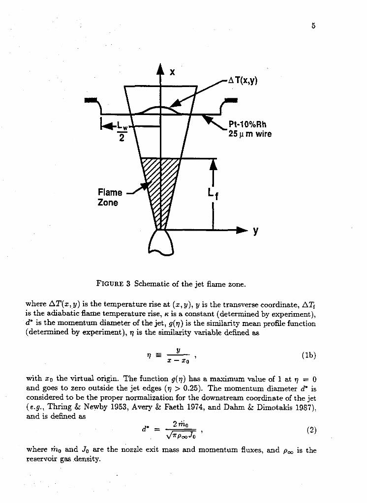
FIGURE 3 Schematic of the jet flame zone.

where AT(x, y) is the temperature rise at (x, y), y is the transverse coordinate, ATf is the adiabatic flame temperature rise, K is a constant (determined by experiment), d' is the momentum diameter of the jet, g(7) is the similarity mean profle function (determined by experiment), r ) is the similarity variable defined as

with 20 the virtual origin. The function g(7) has a maximum value of 1 at 7 = 0 and goes to zero outside the jet edges ( r ) > 0.25). The momentum diameter d* is considered to be the proper normalization for the downstream coordinate of the jet (e.g., Thriig & Newby 1953, Avery & Faeth 1974, and Dahm & Dimotakis 1987), and is defined as

where mo and Jo are the nozzle exit mass and momentum fluxes, and p, is the reservoir gas density.

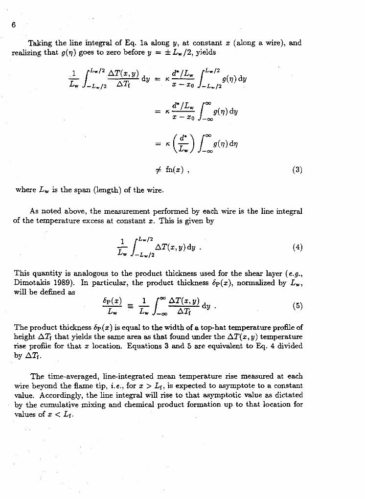
Taking the line integral of Eq. l a along y, at constant x (along a wire), and realizing that g(q) goes to zero before y = -+ Lw/2, yields

where L, is the span (length) of the wire.

As noted above, the measurement performed by each wire is the line integral of the temperature excess at constant x. This is given by

This quantity is analogous to the product thickness used for the shear layer (e.g., Dimotakis 1989). In particular, the product thickness bp(x), normalized by L,, will be defined as

Lw ( 5 )

The product thickness bp(x) is equal to the width of a top-hat temperature profile of height ATf that yields the same area as that found under the AT(+, y) temperature rise profile for that x location. Equations 3 and 5 are equivalent to Eq. 4 divided by ATf.

The time-averaged, line-integrated mean temperature rise measured at each wire beyond the flame tip, i.e., for x > Lr, is expected to asymptote to a constant value. Accordingly, the line integral will rise to that asymptotic value as dictated by the cumulative mixing and chemical product formation up to that location for values of x < Lr.

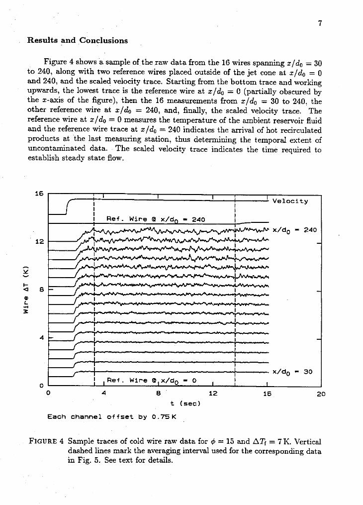
Results and Conclusions

Figure 4 shows a sample of the raw data from the 16 wires spanning x/do = 30 to 240, along with two reference wires placed outside of the jet cone at x/do = 0 and 240, and the scaled velocity trace. Starting from the bottom trace and working upwards, the lowest trace is the reference wire at x/do = 0 (partially obscured by the x-axis of the figure), then the 16 measurements from x/do = 30 to 240, the other reference wire at xldo = 240, and, finally, the scaled velocity trace. The reference wire at zldo = 0 measures the temperature of the ambient reservoir fluid and the reference wire trace at xldo = 340 indicates the arrival of hot recirculated products at the last measuring station, thus determining the temporal extent of uncontaminated data. The scaled velocity trace indicates the time required to establish steady state flow.

Each channel offset b y 0 . 7 5 K

FIGURE 4 Sample traces of cold wire raw data for 6 = 15 and ATf = 7 I<. Vertical dashed lines mark the averaging interval used for the corresponding data in Fig. 5. See text for details.

In the typical data in Fig. 4, note the small delay between the time the jet velocity has reached its steady value and the time the temperature rise is registered in the first wire at x/do = 30. This time corresponds to the time required to flush the jet plenum of its original contents of reservoir fluid and charge it with the F2- bearing jet fluid. Note also the increasing delay required for the reaction head to reach the wires at increasing zldo. The first vertical dashed line, at tl 2 3.3sec, marks the beginning of the time interval over which the data from each wire are to be averaged. The second vertical dashed line, at t2 N 13.6sec, marks the end of the averaging interval, prior to the arrival of the recirculating hot product gases, as registered on the top reference wire at x/do = 240, outside the turbulent jet cone (second trace from the top). Note that the absolute span-averaged temperature change registered by the first wire is approximately 0.5K. Small changes in the vessel temperature in the course of the run, as registered by the reference wire at x/do = 0, are subtracted from the temperature registered by each wire and the difference for each wire is averaged over the selected (tl , t2) time interval for each run. As can be seen from the time-trace of the wire at x/do = 30, the time-averaged mean temperature rise is determinable to a very good fractional accuracy.

The run recorded in Fig. 4 was for a stoichiometric mixture ratio of 4 = 15 and an adiabatic flame temperature rise of ATi = 71<. The stoichiometric mixture ratio 4 represents the mass of reservoir fluid that must be entrained, mixed on a molecular scale, and reacted to completely consume a unit mass of jet fluid. It is defined by

where, for a mixture of N species, the mass fraction, x, is defmed as

with m, equal to the mass of the ith species in the mixture. The resulting averaged data points from the run in Fig. 4 are depicted in the conesponding 4 = 15 trace in Fig. 5.

Data for a number of stoichiometric mixture ratios 4 and an adiabatic flame temperature rise of ATf = 7K were processed, as described above, to produce the plot depicted in Fig. 5. The data correspond to the nondimensional product thickness (Eq. 5) and are plotted versus loglo(x/d*) for the four stoichiometric mixture ratios indicated. The solid line for each set of data is a compound curve fit with a linear least squares fit to the ramp region and a cubic spline fit to the knee region, with the appropriate matching of value, slope, and curvature at the crossover. The flame length Li will be defined as the 99% of maximum 6=/L, point, in the same spirit as the defhition of a 99% boundary layer thickness. The expected

FIGURE 5 Sample plot of product thickness us. loglo(z/d*) for several 4's and an adiabatic flame temperature rise of ATf = 7 K.

increase in the integrated temperature rise is observed, as well as the asymptotic value at the end of the flame tip. The constant temperature level measured by the wires beyond the flame tip is proportional to 4, as can be shown from simple scaling arguments. The results display a linear behavior in the flame region, when plotted in the semi-logarithmic coordinates suggested by the choice of wire spacing, and corroborate the conjecture by Dimotakis mentioned above.

The results of additional experiments will be reported in the near future that address the flame length dependence on Fkynolds number, the transition of the jet from a momentum-dominated to a buoyancy-dominated regime, and the effects of finite rate kinetics (Dahmkiihler number) on mixing in the turbulent jet.

Acknowledgements

We would like to acknowledge the contributions of Godfrey Mungal who was responsible for the initial design of the High Pressure Reactant Vessel and Dan Lang for the data acquisition system and the the wire signal amplifier circuits, discussions and other assistance by Cliff Frieler, David Dowling, Jeff Hall, Paul Miller, Gene Broadwell and Ed Zukoski. Finally, we would like to acknowledge the invaluable contributions of Earl Dahl in the construction and operation of the facility and experiments.

This work was jaintly funded by the Gas Research Institute through Contracts 5083-260-0878 and 5087-260-1467, and the Air Force Office of Scientific Research through Grants 83-0213 and 88-0155.

References

AVERY, J. F. AND FAETH, G. M. [I9741 L'Combustion of a Submerged Gaseous Oxidizer Jet in a Liquid Metal," 15th Annual Combustion Institute, 501-512.

BROADWELL, J. E. [I9821 "A Model of Turbulent Diffusion Flames and Nitric Oxide Generation. Part I," TRW Document No. 38515-6001-UT-00, EERC Final Report, PO No. 18889.

BECKER, H. A. AND YAMAZAKI, S. [I9781 "Entrainment, Momentum and Temper- ature in Vertical Free Turbulent Difusion Flames," Comb. and Flame 33, 123-149.

CHEN, C. J. A N D RODI, W. [I9801 Vertical Turbulent Buoyant Jets. A Review of Experimental Data (Pergammon Press, Oxford).

DAHM, W. J. A. AND DIMOTAKIS, P. E. [I9871 'LMeasurements of Entrainment and Mixing in Turbulent Jets," AIAA J. 25(9), 1216-1223.

DIMOTAKIS, P. E. [I9891 LLTurbulent Free Shear Layer Mixing," AIAA ~ 7 ' ~ Aero- space Sciences Meeting, 9-12 January 1989 (Reno, Nevada), AIAA-89-0262.

DOWLING, D. R. AND DIMOTAKIS, P. E. [1990] "Similarity of the concentration field of gas-phase turbulent jets," J. Fluid Mech. 218, 109.

THRING, M. W. AND NEWBY, M. P. [I9531 LLCombustion length of enclosed turbulent jet flames," 4'h (International) Symposium on Combustion (The Williams and Wilkins Co.), 97.

Appendix C

DIMOTAKIS, P. E. 1991 'LFractals, dinleilsional analysis and similarity, and turbu-

lence," Nonlinear Sci. Today #2/91, pp. 1, 27-31.

acteristic scale and give rise to sets that can be covcrcd by a S h o r t t i m e e x p o s u r e photograph of burning, three-dimenston number N(A) of elements of size A. given hy at surface in a turbulent diffusion flame. Are such turbulent.

N!A) A - " . (,) flow-generated, interfacial surfaces fractal? (Photograph c 1991 by Paul E. Dirnotakis)

Sets whose coverage could bc described in this manner he dubbed fractal, with the exponent D identified as thc associated frarral dimension. See discussion in Mandelbrol 11977. 19821. &d ref. erences therein.

versus A of the cov&ape law of Eq. ( I 1. ~ ~ u i ; a l e n t i y . i t can bc computed from the logarithmic derivative

D = - d lop N(A)

d log A

Strictly speaking. thc dimension D is implicitly defined by Eq. (1). or Eq. ( 2 ) . in the limit of A + 0. This is also thc case for the Hausdofl-Besico~,itcA dimensiur~. defined as the c n t ~ c a l value of the exponent D, where the measure

transitions from zero to infinity. in the limit of A + 0. The summation is to be taken over the set Y with a factor ?(Dl that

-- - -

'Graduate Aeronaut~cal Laboralones Caliiornia lnsillute of Technolog$ Pasa dena. CA 91125

Conrmued on D 37

PUBLISHED BY SPRINGER-VERLAG VOLUME 1, NUMBER 2 1991

Articles in this issue ... I Fractals, Dimensional Analysis and Similarity, and

Turbulence Paul E. Dimorakis

9 Chaos, Contingency, and Convergence Jack Cohen and Ian Srewarf

14 Symmetry, Stability, Geometric Phases, and Mechanical Integrators (Part II) J. E. Marsden, 0. M. O'Reilly, F. J. W,ckl,n, 6. W. Zombro

Complete contents on p. 2

Nonlinear Science Today 1991 Vol. 1. No. 2 27

Dimotakis Continued from p. 1

can depend on the elements used to cover the set (see. for example. Feder 11988, p. 141). In the Mandelbrot 1977 and 1982 discussions. the two quantities are used interchangeably. by considering cases, as he says. for which this equivalence can be accepted.

As Mandelbrot notes 11982. pp. 357-3601, the basic mathe- matical ideas can be traced to earlier proposals and discussions. Equation (2) was essentially used by Pontjagin and Schnirelman in the 30s. and the quantity D defined by Eqs. ( I ) and 12) can be identified with the Kolmo~orov capaciry (Kolmogorov and Tihomirov, 1959). or. as it was subsequently dubbed. the bor- counting dimension. There can be no doubt. however. that it was Mandelbrot who realized the importance of these ideas. brought them to the attention of a community outside that of pure math- ematics, and argued that they should be expected to prove applicable and useful in the description of many physical phenomena. A considerable body of research has appeared on the record in response to his proposals relating to a spectrum of phenomena too numerous to trace.

In the context of many of the phenomena proposed by Man- delbrot to be potentially describable by the fractal power law coverage similarity, however. one must require that Eqs. ( I ) and (2) hold for A not only strictly positive. but over some nonvan- ishing range of scales A , i.e.. for

O < A m,,, S A S A n m x . (4)

This is a necessary assumption if one is to derive many of the benefits of this analysis. It will also prove important on another score

Specifically, to return to the basic proposal. it is important to note that as regards the description of physical entities in which A has units. Eq. ( I ) is nor dimensional!\. correcr; only a dimensionless group can be equal to a pure number. Of course. one could argue that a proportionality constant C is implicit in Eq. (I) , 1.e..

N(A) = C K D . ( 5 )

Such a constant would be dimensional, however. with units as dictated by those of A and the value of D, i.e.. C = fn(D). In using Eq. ( 5 ) as an implicit definition of D, in other words, in which D is the independent variable. the "constant" of propor-

tionality C is not a constant at all and hides important scaling information.

To illustrate the point, consider a set representing a surface in a d-dimensional (Euclidean) space. for example, fixed threshold crossing of a scalar time trace. or linear image (d = I); isoscalar contours of a scalar field. e.g.. c1x.j) = c,,, in a planar image Id = 2): or isoscalar surfaces, e.g., c(x,j,:) = c,,, of a scalar field in three dimensions Id = 3) . Consider a volume given by L< in each case, where L is the (linear) extent of the space spanned by the data. The total number of A-sized elements that can fit in this space is given by (LIA)~.: The total coveragc N,,(A) of the set can then be expressed as the fraction of the number of A-elements covering the set, times the total number of A-elements in the d-dimensional (data) space, i.e..

The proposal that N,(A) = is then equivalent to a dependence of the coverage fraction on A , i.e.. the probability that a A-element covers a portion of the set, given by

F, ( A ) = A " - ~ " . (7)

Since F, ( A ) is a probability and therefore dimensionless. Eq. 7 requires that A must be scaled by some like-dimensioned quantity, or characteristic scale. A,. i.e..

We can combine this with Eq. 6 to yield what is implicit in thc original equation, namely.

In this expression, the now dimensionless constant F,, is equal to the required fraction of set-covering elements of size A = A,,. provided, of course. the characteristic scale A, falls within the (A ,,., A,,,) interval in which Eq. 9 applies. While, in principle, the factor F, could be absorbed in a redefined A,, it is useful to retain it; the characteristic scale A, might well be definable on some other physical basis quite independently of a fit to the coverage of the set of interest using Eq. 9.

+Barring edge effects. whtch. however. can be eliminated in any o f a number o f way-for example. by considering A's that are exact binary rubmulliples o f L, i . e . An = LIZ"

28 1991 Vol. 1, No. 2 Nonlinear Science Today

As an aside, it might appear thai Eq. (3). the Hausdorff- Besicovitch expression for D, is not subject to the same difficulty. Strictly speaking, it is dimensionally correct as it stands. Nevertheless, one would prefer not to be using a measure that is dimensional (with units that depend on the value of D), or to be taking the limit with a dimensional A + 0, to determine the critical value of D. Instead, one would prefer a measure based on a scaled A, e.g., A(AIA,; D l , with D computed a s the critical exponent in the limit of AIA, - 0. Again. in other words, there is a need for a characteristic scale A,. even if not as manifestly as with the box-counting coverage expression of Eq. ( I )

These observations have an interesting consequence. Returning to Eqs. ( l ) , (5). or (9). we see that they can be

expected only to apply to processes that observe a characteristic scale A,. The resulting coverage function NiAl could then depend strongly on this characteristic scale, or not. depending on the value of the dimension exponent D. More imponantly, however. the coverage of sets generated by processes that do not possess such a characteristic scale cannot be expected to be described by these equations.

Turning to the more specific question. an area in which there have been many attempts to apply power law fractals is ". . . the grand chapter of Physics, the study of turbulence in fluids" [Mandelbrot, 1977, p. 1451-the dynamics. in other words. of high Reynolds number fluid motion. Turbulent-flow-generated sets, especially at high Reynolds numbers. are known to exhibit a host of similarity properties. Thesc can be expected to hold over a large range of space and time scales that are bracketed by

A,,, - 6. i10a)

the outer flow scale, and I..?\ 184

the inner Kolmogorov [1941a] scale, in which u is the kinematic viscosity and E is the mean dissipation rate of the kinetic energy per unit mass. At high Reynolds numbers Re. the bounds of this (inertial) range are in the ratio

"mln & K

This potentially very largc similarity range would seem to provide a promising arena for thc Mandelbrot fractal proposals. Sets generated by turbulent flow processes that have been analyzed in this light include selected velocity component time traces, estimates of the local energy dissipation and its fluctuations, temporal as well as spatial scalar fluctuations and isoscalar surfaces. etc. The recent review by Sreenivasan (19911 can be consulted for a discussion and references.

Let us examine this proposal in view of some of the similarity properties in the inertial range of scales and the preceding discussion

In his first and second similarity hypotheses. Kolmogorov 11941al proposed that the only dynamically important quantity at a scale A = 2vIk within the range of Eq. (4). with the identifi- cations in Eqs. (10). is the mean dissipation rate F . This proposal immediately leads to the celebrated Kolmogorov -/i spectrum by dimensional analysis, i.e..

E(k) I t l ' z k - i 3 K (12~)

where C, is a (dimensionless) constant of proportionality of order unity. The right-hand side is the only group that can be formed with c and k that has the requisite dimensions.

Physically, the first and second Kolmogorov hypotheses are equivalent to assuming that the dynamics of the turbulent strain-

ing motions that take an eddy of a scale A , to a scale AZ. for

6 B A , > A 2 B A K ,

depend only on the local scale and therefore only on the ratio A,/A,. In particular. they are equivalent to assuming that the dynamics do not depend on the ratio of the local scale A to the outer scale 6. the inner scale A, or any orher scale.

In subsequent refinements by Kolmogorov [1962], Oboukhov 119621. and others, the kinetic energy dissipation rate E = ~ ( x , r ) was accommodated as the local, intermittent field that it is. This introduced the outer scale 6 as a scale weak/! admissible in the dynamics, resulting in small corrections to the - % spectrum. Specifically, with a log-normally distributed r(x,r), the energy specttum becomes

~ ( k ) = cK ~ 2 ' 3 ( k 6 ) - ~ , 4 )(-5r3, (I2h)

where p is the intennittency exponent. estimated to be in the range of 0.2 < p < 0.5 (e.g.. Monin and Yaglom 11975, p. 6421). Significantly. the difference between Eqs. (12a) and (12b) is too small to be discernible experimentally. At least by this measure. we may conclude that the Kolmogorov 11941aI hypothesis of scale independence. that leads to the - s/? spectrum law. must very nearly be right.

This conclusion has consequences. in light of the preceding discussion of the need for a characteristic scale to exist. if the power law fractal similarity is to describe the coverage. In the

the fractal dimension exponent D, f i r cov;rage of 't'hree- dimensional sets is to be assigned values in the range of D, = 2.36 ? 0.05. as was suggested. for example, by Sreenivasan 11991, p. 556). This is also a value close to D, = X/i that Man- delbrot suggests "is reducible to the Kolmogorov theory and the empirical spectra.": which he also argues corresponds to a value of Dl = % for planar sections [Mandelbrot 1977, p. 521.

We note here that. implicit in the assignment of both the rc- ported experimental estimate of D, = 2.36 ? 0.05 of Sreenivasan, as well as the correspondence between the value of D, = 8/~ and Dl = % proposed by Mandelbrot as applicable to isoscalar surfaces. is the relation

d , - D d , = d l - D ,,. (13)

where d, and d, denote the topological dimension, c.g.. D, = D, + I and D, = D, + 2. as was assened by Sreenivasan and Meneveau 11986, Sec. 2.21-recall also Eqs. (8) and (9). Spe- cifically. in the case of the experimental values reported, the value of D, cited was inferred from measurements of one- dimensional (d = I ) or two-dimensional (d = 2) data, assuming Eq. (13). A suggestion to that effect had previously been made by Mandelbrot. whom Sreenivasan and Meneveau 119861 cite as a reference for this. and who says that "it is 'almost sure' " that the intersection of a three-dimensional surface with a plane yields a dimension Dl = D, - I [Mandelbrot, 1982. p. 1351, especially if the three-dimensional surface of interest is irregular (ibid.. p. 136). The latter proviso would of course be satisfied in the ease for an isoscalar surface in turbulence. for example (see also the discussion in Mandelbrot 11976. p. 124; 1977, p. 521 cited above). We will return to this point below.

Accepting Eq. (13) at face value for now, we can argue that such values for D, for an isoscalar surface. for example, are too far from the topological dimension of a three-dimensional object, i.e.. D, = 3. and. despite Mandelbrot's assertion. that the resulting dependence of the coverage function N,iA) on whatever

tlr is not clear whether Mandelbrot. ~n his reference here lo "the Kolmogorov theory and the emp~rlcal spectra." IS thtnktng of the original (1941a) arguments leading lo the -'/I spectrum IEq. i I2a). or the revised (1962) proposals that lead to Eq. i l2b) l .

Nonlinear Science Today 1991 Vol. 1 , No. 2 29

characteristic scale A, is used i n E q . (9) is too strong to be consistent with turbulent flow inertial range similarity. This conclusion can be reached by considering the properties of an isoscalar surface and its proposed (power law) fractal coverage N3(A), assuming that

Ao " 6 , (14) as one might in view of the turbulent cascade process from larger to smaller scales. If we consider, for example, two gedanken experiments in the same type of flow. arranged to generate the same inner scales A,, but with outer scales 6, and differing by, say, a factor of 10. and compare the coverage N,(A) at a fixed scale A, say, for A = IOA, d 6, .6 , . The analysis of such a comparison is beyond the purposes of the present brief, informal discussion and is not included here

This argument was recently noted in Miller and Dimotakis [19911, who did not find Eq. (1) [or. equivalently. Eq. (9)) applicable to measurements of temporal isoscalar intersections at a fixed point, or to spatial measurements derived from linear images, in the far field of turbulent jets where it had previously been reported to apply (e.g., Sreenivasan and Meneveau [1986]). In a note added in proof, Sreenivasan [I9911 suggested that the discrepancy could be attributable to the fact that Miller and Di- motakis analyzed temporal data. As noted above. however. not only had such behavior been reported previously for temporal data," but in their discussion Miller and Dimotakis included measurements and the analysis of temporal. spatial. as well as spatio-temporal (streak image) data. with similar results.

Briefly, to cover a total of N, transitions in a one-dimensional record of length L, we must find

for A + 0 N1(A) + {:A for A > 6 .

The small-scale limiting behavior can be understood by appreci- ating that, once the covering element scale A has decreased below the shortest separation between threshold transitions in the scalar trace, the total number of elements of size A required to cover those transitions becomes equal to the total number N, of transitions in the record of length L.

The large-scale limiting behavior can be understood by appre- ciating that e v e v covering element of size A much larger than the outer scale 6 will cover transitions and. therefore. the total number of elements required to cover those transitions must tend to the total number of elements LIA that can fit in the record. In other words, we must have F,(A) -1 for A > 6 (cf. Eq. 6) . It is also easy to appreciate that. for typical traces derived from turbulent flow, the number of elements N,(A) needed to cover the corresponding sets would only gradually approach the limiting values in Eq. (15). for small and large A.

In view of the above and Eq. ( 2 ) . we must have. for one- dimensional isoscalar data. that

0 for A < As I for A > 6 . (16)

where A, is the Batchelor 119591 scalar diffusion scale (below which the isoscalar surface can be regarded as differentiable). and that, therefore, the exponent D , cannot be treated as a constant.

While it may be a minor point. it should be noted that if the measurements are alias-free with some margin, i.e.. if they have been sampled at a frequency comfortably higher than the Nyquist

0 -5 -4 3 -2 -1 0

laglOii/ml

Figure 1: Coverage N,(A) derived from tempgral data of jet fluid concentration crossings of the local c, measured on the axis of a turbulent jet at xld = 100 and a Reynolds number of 1.15 x 10'. The scale A here is converted to meters. Data from Miller and Dimotakis [1991].

frequency. and sufficiently noise-free, N(A) should tend to a constant at the smallest values of A resolved by the data [for the reasons stated in reference to Eq. (IS)] whether or not the smallest scale of the physical process has been resolved. It should also tend to the corresponding limit at large A if the record length L spans a sufficient number of outer flow scales. Accordingly. we can always expect the limits in Eq. (16) to he attained by the analysis of proper data.

Of course. the preceding alone does not preclude, a priori, the existence of a D,(A) that osculates a constant value over a range of scales A,

AB < AmIn < A < Amax < 6 , in the case of isoscalar surfaces. That is rendered unlikely by the additional requirement for a characteristic scale A, appropriate to that range, as noted above.

Rewriting Eq. (2). we conclude that, in general, we must allow the exponent D to he a function of A , i.e..

as suggested in Miller and Dimotakis. In the analysis of their turbulent jet fluid scalar data, they find a D,(A) smoothly rising from 0 to I , over a range of jet Reynolds numbers, 3.0 x 103 s Re S 2.4 x lo4. with no indication of any preferred intermediate value. They also report that the observed D,(A) is very close to one derived from a simple model process in which scalar threshold transitions are log-normally spaced.

Figure I depicts N,(A), as required to cover transitions of the scalar jet fluid concentration trace c(r). of a threshold set at the local mean ?,* on the axis of a turbulent jet in water, at xld = 100. and a Reynolds number of 1.15 x lo4. In this plot, the covering element scale A was converted to an equivalent spatial extent, measured in meters. to facilitate comparison with other temporal data, at both higher and lower Reynolds numbers (cf. Miller and Dimotakis 11991. Fie. 41). The outer scale (local iet .. diameter) is estimated to be 6 = 0.1 I m, i.e., loglo(6/m) =

*Nore reference lo the use of Tiglor'r frozen flow hypothes,~ in Sreenivaran. Ramshankar nnd Meneveau. 11989. Table I ] . Note (dl. where the 'The Imponant tirue of rhe choice of the lhre>hold was addressed m Miller and Sreenivasan and Meneveau 119861 jet data are cmd. Dlmotakii 119911. l h e reader is referred lo that d~rcurr~on for funher delailr.

30 1991 Vol. 1, No. 2

Figure 2: Logarithmic derivative D, (h /m) . Eq. (17). of the coverage N,(h) plotted in Figure 1

- 1.0. As can be seen, the computed coverage observes the required limits noted in Eq. (15).

Figure 2 plots the logarithmic derivativeD,(h). computed from the N,(A) coverage plotted in Figure 1. Note that the measured Dl(A) + 0, at the smallest scales, and D,(A) + I for A - 6 . or larger, as required. The dashed line in Figure 2 marks the level D, = 0.36. The latter was the value reported to have been derived from direct measurements of one-dimensional temporal data by Sreenivasan and Meneveau [ 19861. It would also be the value derived from the previously cited estimate of D3 = 2.36 if the assertion that D, = D l + 2 is accepted [Eq. (13)]. However. while the assertion of Eq. (13) may be true in special cases, it must in general be false, as will be argued below.

Consider an isotropic random surface in three dimensions, which we accept as possessing a fractal dimension D,. and its intersection with a plane. yielding a two-dimensional curve, which we will also accept as possessing a fractal dimension DZ. Using the two-dimensional curve. we generate (extrude) a cylindrical surface by translating the two-dimensional curve along a direction pemendicular to its plane. As Feder 11988. Fie. 13.1 and relateb discussion] notes. ihc dimension ofthe resulsng cylindrical surface. which has vcrv different mace-filling Drooer- - . . ties, is given by D 2 + I . Equivalently. we can expect the required coverage fraction F,(A). cf. Eqs. 6 . 8, and 9. to be different for the original three-dimensional isotropic surface. vs. the generated cylindrical surface

This suggests that for a random surface in three-dimensions. of dimension D,, and a planar sectlon of the same surfacc of dimension D2. we can expect, in general.

D, f D2 + I (18)

(analogously, for curves that are originally planar of dimension DZ versus linear cuts yielding intersections of dimension D, ) .

Is the implication that there can be no (power law) fractals'! Not at all.

To return to the earlier point on similarity and dimensional analysis, the inference that should be drawn is that a (power law) fractal coverage relation requires a characteristic scale. Without, that, and as opposed to the original proposals, we cannot write Eq. ( I ) dimensionally correctly. Conversely. processes that do possess relevant characteristic scales could exhibit (power law) fractal behavior.

What is then the relevant 'characteristic scale for the triadic Cantor set (e.g., Mandelbrot 11977, p. 981). often described as

Nonlinear Science Today

self-similar, for example? It is easy to appreciate that, for the triadic Cantor set. the

characteristic scale is the original length L that is successively subdivided into thirds. i.e., A, = L in Eq. 9. The resulting set is obviously nor self-similar at all scalings: it is not, the same if we cut the original length L in half. for example. It is also not self-similar homogeneously; successive subdivisions d o not en- dow the middle third of the original L with any Cantor "dust." Only the first and last third subsegments of any (sublsegment of the Cantor set are similar. This represents a rather restricted similarity scaling, which is pegged to the original length L and a coverage phased with respect to the original segment. The oscillations in the calculations of Smith et al. [1986]. as well as in the spectmm of the triadic Cantor set.? can be understood in this light.

Accepting that the geometry of coastlines may be describable by a power law fractal relation. for example (cf. Feder [1988, Fig. 2.71). one can think of several candidate characteristic scales that could be relevant. Potentially. these range from buoyant scales of the motion within the earth's mantle, responsible for tectonic motion on continental dimensions. to ocean wave scales at intermediate topography scales. to rock grain boundary and fracture scales. and below. as appropriate for microscopic and submicrosco~ic stochastic eeometrv scales. One could imaeine - the application of Eq. (9). corresponding to each of these separate characteristic scales. with. ootentiallv. a different valuc of the exponent D for each one.

In the context of fluid mechanics and turbulence. this is also not to say that (power law) fractal relations and constant fractal dimension exponents are ruled out. The arguments here attempt to address issues arising in fully developcd. turbulent flow in the intermediate. inertial range of scales. where power law fractals have been proposcd to apply. Converscly. however. isoscalar surfaces that. for example, demark the boundaries of a turbulent region and even may serve as the definition of the outer scale 6 are susceptible to dynamics that are obviously not independent of a characteristic scale. namely, the outer scale 6. Such interfaces would then appear to possess the necessary condition for a power law fractal description to be applicable and may indeed bc found to display such behavior. It would then. howcvcr. be surprising if the resulting fractal dimension exponents were found to bc universal. i.e.. independent of the details of thc flow geometry. Reynolds number, Schmidt number. etc.

More generally, however. one might accept the need to ana- lyze stochastic geometric data. using the tools of fractal analysis. without requiring that they conform to power law similarity relations. Non-power-law stochastic geometry similarity could be useful for analogous purposes, as was sugeested by Miller and Dimotakis. who instead found loe-normal similarity a~plicable in their analysis of turbulent jet flujd scalar fluctuatibn'records.

Indeed. the log-normal distribution was originally proposed by Kolmogorov (1941b) to describe the self-similar fragmentation process resulting from successive rock crushings.

Acknowledgments Many people have contributed. over some timc. to thc evolution of these ideas. Over the last few years. I would like to acknowledge the many discussions at Caltech with Paul Miller. with whom the experiments cited here were conducted. as well as Tony Leonard. Without wishing to imply endorsement. I would also like to acknowledge some recent discussiuns with Uriel Frisch and Lany Sirovich that spawned improvements in the exposition of the arguments presented here.

Nonlinear Science Today 1991 Vol. 1, No. 2 31

References G. K. BATCHELOR 119591 Small-scale variation of convected quantities

like temperature in turbulent fluid. Part 1. General discussion and the case of small conductivity, J. FluidMech. 5, 11S133.

J. FEDER 119881 Fmcrals. Plenum Press, New York. A. N. K~LMOGOROV [194La] Local structure of turbulence in an incom-

pressible viscous fluid at very high Reynolds numbers, Dokl. A M . Nauk SSSR 30, 299. Reprinted in: Us@. Fiz. Nouk 93, 47&481 (1967). Translated into English in: Sov. Phys. Usp . 10(6), 73&736 (1968).

A. N. Kolmogorov [1941b] The logarithmically normal law of distribution of dimensions of particles when broken into small parts. A M . Nauk SSSR 31(2), 99-101. Translated into English by V. Levin in NASA-TI F-12. 287 (1969).

A. N. KOLMOGOROV [I9621 A refinement of previous hypotheses concerning the local structure of turbulence in a viscous incompressible fluid at high Reynolds number, J. Fluid Mech. 13, 82-85.

A. N. KOLMOGOROV AND V. M. TIHOMIROV (19591 c-entropy and E-capacity of sets in functional spaces. Am. Morh. Soc. Transiarions. 1961 (Section II), 277-364.

B. MANDELBROT 119761 Intermittent turbulence and hactal dimension: kurtosis and the spectral exponent Y3 + B. Turbulence and rhe Navier Stokes Equations. Conf Proc. (U. Paris-Sud. Orsay), 12-13 June 1975, Lecture Notes in Mnrhemrics No. 565. Eds. A. Dold, B. Eck- mann. Sorineer-Vedae. New York. on. 121-145.

H B MA~DE;BROT [ 1di71 Frutruls ~ o r m Chanze, and D#mcnvton W H Freeman & Co . San Franc~sco.

B. B. ~ ~ A N D C . I . U R O T 1 I9821 The Fru<?ol Gromrrq o/ Nurur?. W H Freeman & Co., New York.

P. L. MILLER AND P. E. DlMOTAKlS [I9911 Stochastic geometric properties of scalar interfaces in turbulent jets, Phys. Fluids A 3(1), 168- 177.

A. S. MONIN AND A. M. YAGLOM [I9751 Sraristical Fluid Mechnnics: Mechnnics of Turbulence II, 1. Lumley (ed.). MIT Press. Cambridge, MA.

A. M. OB~UKHOV 119621 Some specific features of almaspheric turbulence. J. FluidMech. 13, 77-81.

L. A. SMITH, J-D. FOURNIER. AND E. A. SP~EGEL 119861 Lacunarity and intermittency in fluid turbulence, Phys. Lerr. A 114, 465468.

K. R. SREENIVASAN 119911 Fractals and multifractals in fluid turbulence. Ann. Rev. FluidMech. 23, 539-600.

K. R. SREENIVASAN AND C. MENEVEAU (19861 The hactal facets of turbulence, I . FIuidMech. 1'13, 357-386.

K. R. SREENIVASAN, R. RAMSHANKAR. AND C. MENEVEAU (19891 Mix- ing, entrainment and fractal dimensions of surfaces in turbulent flows, Proc. Roy. Soc. London A 421, 79-108.

graduate aeronautical laboratories california institute...

Documents