Gradient-based training of Gaussian Mixture Modelsfor High-Dimensional Streaming DataAlexander Gepperth 

Fulda University of Applied Sciences: Hochschule FuldaBenedikt Pfülb  ( benedikt.pfuelb@cs.hs-fulda.de )

Fulda University of Applied Sciences: Hochschule Fulda https://orcid.org/0000-0002-0108-1936

Research Article

Keywords: Gaussian Mixture Model, Stochastic Gradient Descent

Posted Date: July 26th, 2021

DOI: https://doi.org/10.21203/rs.3.rs-369722/v1

License: This work is licensed under a Creative Commons Attribution 4.0 International License.  Read Full License

Version of Record: A version of this preprint was published at Neural Processing Letters on August 17th,2021. See the published version at https://doi.org/10.1007/s11063-021-10599-3.

Neural Processing Letters manuscript No.(will be inserted by the editor)

Gradient-based training of Gaussian Mixture Models

for High-Dimensional Streaming Data

Alexander Gepperth · Benedikt Pfulb

Received: date / Accepted: date

Abstract We present an approach for efficiently training Gaussian Mixture Model(GMM) by Stochastic Gradient Descent (SGD) with non-stationary, high-dime-nsional streaming data. Our training scheme does not require data-driven param-eter initialization (e.g., k-means) and can thus be trained based on a randominitial state. Furthermore, the approach allows mini-batch sizes as low as 1, whichare typical for streaming-data settings. Major problems in such settings are un-desirable local optima during early training phases and numerical instabilitiesdue to high data dimensionalities. We introduce an adaptive annealing procedureto address the first problem, whereas numerical instabilities are eliminated by anexponential-free approximation to the standard GMM log-likelihood. Experimentson a variety of visual and non-visual benchmarks show that our SGD approachcan be trained completely without, for instance, k-means based centroid initializa-tion. It also compares favorably to an online variant of Expectation-Maximization(EM) – stochastic EM (sEM), which it outperforms by a large margin for veryhigh-dimensional data.

Keywords Gaussian Mixture Model · Stochastic Gradient Descent

1 Introduction

This contribution focuses on Gaussian Mixture Model (GMM), which represent aprobabilistic unsupervised model for clustering and density estimation, allowingsampling and outlier detection. GMMs have been used in a wide range of sce-narios, see [18]. Commonly, free parameters of a GMM are estimated using theExpectation-Maximization (EM) algorithm [7], which does not require learningrates and automatically enforces all GMM constraints. A popular online variant isstochastic EM [2], which can be trained mini-batch wise and is thus more suitedfor large datasets or streaming data.

Fulda University of Applied SciencesLeipziger Str. 123, 36037 FuldaE-mail: {alexander.gepperth,benedikt.pfuelb}@cs.hs-fulda.de

2 Alexander Gepperth and Benedikt Pfulb

1.1 Motivation

Intrinsically, EM is a batch-type algorithm. Therefore, memory requirements canbecome excessive for large datasets. In addition, streaming-data scenarios requiredata samples to be processed one by one, which is impossible for a batch-typealgorithm. Moreover, data statistics may be subject to changes over time (conceptdrift/shift), to which the GMM should adapt. In such scenarios, an online, mini-batch type of optimization such as SGD is attractive since it can process samplesone by one, has modest, fixed memory requirements, and can adapt to changingdata statistics.

1.2 Related Work

Online EM is a technique for performing EM mini-batch wise, allowing to pro-cess large datasets. One branch of previous research [20,16,4] has been devoted tothe development of stochastic Expectation-Maximization (sEM) algorithms thatreduce to the original EM method in the limit of large batch sizes. The variantpresented in [2] is widely used due to its simplicity and efficiency for large datasets.Such approaches come at the price of additional hyper-parameters (e.g., step size,mini-batch size, step size reduction), thus removing a key advantage of EM overSGD. Another approach is to modify the EM algorithm itself by, e.g., includingheuristics for adding, splitting and merging centroids [30,10,24,3,26,15,29]. Thisallows GMM-like models to be trained by presenting one sample after another.Models of this type work well in several application scenarios, but their learningdynamics are impossible to analyze mathematically. They also introduce a highnumber of parameters. Apart from these works, some authors avoid the issue ofextensive datasets by determining smaller “core sets” of representative samplesand performing vanilla EM [11].SGD for training GMMs has, as far as we know, been recently treated onlyin [13,14]. In this body of work, GMM constraint enforcement is ensured byusing manifold optimization techniques and re-parameterization/regularization,thereby introducing additional hyper-parameters. The issue of local optima isside-stepped by a k-means type centroid initialization, and the used datasets arelow-dimensional (36 dimensions).Annealing and Approximation approaches for GMMs were proposed in [28,23,22,8]. However, the regularizers proposed in [28,22] significantly differ from ourscheme. GMM log-likelihood approximations, similar to the one used here, are dis-cussed in, e.g., [23] and [8], but only in combination with EM training. A similar“hard assignment” approximation is performed in [27].GMM Training in High-Dimensional Spaces is discussed in several publica-tions: A conceptually very interesting procedure is proposed in [12]. It exploits theproperties of high-dimensional spaces in order to achieve learning with a number ofsamples that is polynomial in the number of Gaussian components. This is difficultto apply in streaming settings, since higher-order moments need to be estimatedbeforehand, and also because the number of samples is usually unknown. TrainingGMM-like lower-dimensional factor analysis models by SGD on high-dimensionalimage data is successfully demonstrated in [25]. This approach avoids numericalissues, but, again, sidesteps the local optima issue by using k-means initializa-

Gradient-based training of GMMs for High-Dimensional Streaming Data 3

tion. The numerical issues associated with log-likelihood computation in high-dimensional spaces are generally mitigated by using the “logsumexp” trick [21],which is, however, insufficient for ensuring numerical stability for particularly high-dimensional data, such as images.

1.3 Goals and Contributions

The goals of this article are to establish GMM training by SGD as a simpleand scalable alternative to sEM in streaming scenarios with potentially high-dimensional data. The main novel contributions are:

– a proposal for numerically stable GMM training by SGD that outperformssEM for high data dimensionalities,

– an automatic annealing procedure that ensures SGD convergence without priorknowledge of the data (no k-means initialization) which is beneficial for stream-ing data,

– a computationally efficient method for enforcing all GMM constraints in SGD,– a convergence proof for the annealing procedure.

Additionally, we provide a TensorFlow implementation.1

2 Gaussian Mixture Models

GMMs are probabilistic models that try to explain the observed data X = {xn} byexpressing their density as a weighted mixture of K Gaussian component densitiesN (x;µk,Pk)≡Nk(x):

p(xn) =K∑

k=1

πkNk(xn). (1)

Here, we parameterize Gaussian densities by precision matrices Pk =Σ−1

k in-stead of covariances Σk. The component weights πk represent another set ofGMM parameters, which modulate the overall influence of each Gaussian den-sity. For a derivation of eq. 1, we must introduce the probabilistic foundations ofGMMs. GMMs assume that each observed data sample {xn} is drawn from oneof the Gaussian component densities Nk. The selection of this component den-sity is assumed to depend on an unobserved (and unobservable) latent variable

zn ∈ {1, . . . ,K} which follows an unknown distribution. This is formalized for aGMM with K components by formulating the complete-data likelihood for a singledata sample as:

p(xn, zn) = πznNzn

(xn), (2)

Since the latent variables are, by construction, unobservable, we must marginalizethem out of eq. 2 in order to obtain an expression suitable for optimization. Thisgives us the incomplete-data likelihood for a single data sample xn:

p(xn) =

K∑

k=1

p(xn, k), (3)

1 https://gitlab.cs.hs-fulda.de/ML-Projects/sgd-gmm

4 Alexander Gepperth and Benedikt Pfulb

which depends on observable quantities only. Please compare this to eq. 1. Theincomplete-data likelihood for all samples is thus given by:

p(X) =∏

n

p(xn) =∏

n

∑

k

p(xn, k) =∏

n

∑

k

πkNk(xn), (4)

where we have inserted eq. 2 in the last step. Passing to the log-domain (asit is common for probabilistic models), we obtain the total incomplete-data log-

likelihood for all observed data samples:

L = log p(X) =∑

n

log∑

k

πkNk(xn). (5)

The function L contains only observable quantities and is a suitable loss func-tion for optimization. For convenience and numerical stability, the sum is usuallyreplaced by an expectation, and we follow this convention:

L = En

[

log∑

k

πkNk(xn)

]

. (6)

Please note that L represents the likelihood of the observed data under the GMMwith current parameters, and must therefore be maximized to obtain a betterexplanation of the data.

2.1 GMM Constraint Enforcement for SGD

GMMs require the mixture weights to be normalized:∑

k πk =1 and the precision

matrices to be positive definite: x⊤Pkx≥ 0 ∀x. These constraints must be explic-itly enforced after each SGD step:Weights πk are adapted according to [13], which replaces them by other freeparameters ξk from which the πk are computed so that normalization is ensured:

πk =exp(ξk)

∑

j exp(ξj). (7)

Diagonal precision matrices are re-parameterized as Pk =D2k, with diagonal

matrices Dk (Cholesky decomposition). They are, therefore, guaranteed to be

positive definite. Hence, detΣk =detP−1

k =(

det(D2k))−1

=(

Tr(Dk))−2

can becomputed efficiently. Since we are dealing with high-dimensional data, precisionmatrices are always taken to be diagonal, since full matrices would be prohibitivew.r.t. memory consumption and the number of free parameters.

Full precision matrices are treated here for completeness’ sake, since they areinfeasible for high-dimensional data. We represent them as a spectral decompo-sition into eigenvectors vi and eigenvalues λ2

i : Pk =∑

i λ2iviv

⊤i , which ensures

positive-definiteness. This can be seen from detΣk =detP−1

k =∏

i λ−2

i . In orderto maintain a correct representation of eigenvectors, these have to be orthonor-malized after each SGD step.

Gradient-based training of GMMs for High-Dimensional Streaming Data 5

2.2 Max-Component Approximation for GMM

The log-likelihood eq. 5 is difficult to optimize by SGD due to numerical problems(mainly underflows and resulting divisions by zero) for high data dimensionalities.This is why we intend to find a lower bound that we can optimize instead. A simplescheme is given by

L=En

[

log∑

k

πkNk(xn)

]

≥En

[

logmaxk(

πkNk(xn))

]

= L=En

[

log(

πk∗Nk∗(xn))

]

(8)

where k∗ =argmaxk πkNk(xn). This is what we call the max-component approx-

imation of eq. 8. In contrast to the lower bound that is constructed for EM-typealgorithms, our bound is usually not tight. Nevertheless, we will demonstrate laterthat it is a very good approximation when data are high-dimensional. The ad-vantage of L is the elimination of exponentials causing numerical instabilities.The “logsumexp” trick is normally employed with GMMs to rectify this by fac-toring out the largest component probability Nk∗ . This mitigates but does notavoid numerical problems when distances are high, a common occurrence for highdata dimensions. To give an example: we normalize the component probabilityNk = e−101 (using 32-bit floats) by the highest probability Nk∗ = e3, and we ob-tain Nk

Nk∗

= e−104, which produces an underflow respectively NaN values.

2.3 Undesirable Local Optima in SGD Training

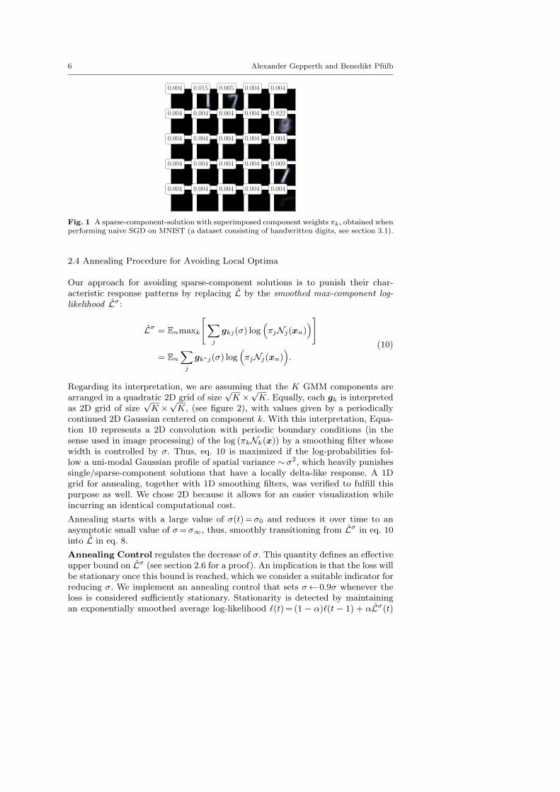
A crucial issue when optimizing L (and indeed L as well) by SGD without k-means initialization concerns undesirable local optima. Most notable are the sin-gle/sparse-component solutions, see figure 1. They are characterized by oneor several components {ki} having large weights, with centroid and precision ma-trices given by the mean and covariance of a significant subset Xki

⊂X of thedata X: πki

≫ 0, µki=E[Xki

], Σki=Cov(Xki

), whereas the remaining compo-nents k are characterized by πk≈ 0, µk =µ(t=0), Pk =P (t = 0). Thus, theseunconverged components are almost never the best-matching units (BMUs) k∗.

The max-operation in L causes gradients like ∂L∂µk

to contain δkk∗ :

∂L∂µk

= En [Pk (xn − µk) δkk∗ ]

∂L∂Pk

= En

[(

(Pk)−1 − (xn − µk)(xn − µk)

⊤)

δkk∗

]

∂L∂πk

= π−1

k En [δkk∗ ] .

(9)

This implies that the gradients are non-zero only for the BMU k∗. Thus, thegradients of unconverged components vanish, meaning that component parametersremain in their unconverged state.

6 Alexander Gepperth and Benedikt Pfulb

Fig. 1 A sparse-component-solution with superimposed component weights πk, obtained whenperforming naive SGD on MNIST (a dataset consisting of handwritten digits, see section 3.1).

2.4 Annealing Procedure for Avoiding Local Optima

Our approach for avoiding sparse-component solutions is to punish their char-acteristic response patterns by replacing L by the smoothed max-component log-

likelihood Lσ:

Lσ = Enmaxk

[

∑

j

gkj(σ) log(

πjNj(xn))

]

= En

∑

j

gk∗j(σ) log(

πjNj(xn))

.

(10)

Regarding its interpretation, we are assuming that the K GMM components arearranged in a quadratic 2D grid of size

√K ×

√K. Equally, each gk is interpreted

as 2D grid of size√K ×

√K, (see figure 2), with values given by a periodically

continued 2D Gaussian centered on component k. With this interpretation, Equa-tion 10 represents a 2D convolution with periodic boundary conditions (in thesense used in image processing) of the log (πkNk(x)) by a smoothing filter whosewidth is controlled by σ. Thus, eq. 10 is maximized if the log-probabilities fol-low a uni-modal Gaussian profile of spatial variance ∼σ2, which heavily punishessingle/sparse-component solutions that have a locally delta-like response. A 1Dgrid for annealing, together with 1D smoothing filters, was verified to fulfill thispurpose as well. We chose 2D because it allows for an easier visualization whileincurring an identical computational cost.

Annealing starts with a large value of σ(t)=σ0 and reduces it over time to anasymptotic small value of σ=σ∞, thus, smoothly transitioning from Lσ in eq. 10into L in eq. 8.

Annealing Control regulates the decrease of σ. This quantity defines an effectiveupper bound on Lσ (see section 2.6 for a proof). An implication is that the loss willbe stationary once this bound is reached, which we consider a suitable indicator forreducing σ. We implement an annealing control that sets σ← 0.9σ whenever theloss is considered sufficiently stationary. Stationarity is detected by maintainingan exponentially smoothed average log-likelihood ℓ(t)= (1 − α)ℓ(t − 1) + αLσ(t)

Gradient-based training of GMMs for High-Dimensional Streaming Data 7

Fig. 2 Visualization of Gaussian smoothing filters gk used in annealing, of width σ, for threedifferent values of σ. The gk are placed on a 2D grid, darker pixels indicate larger values.Over time, σ(t) is reduced (middle and right pictures) and the Gaussians approach a deltapeak, thus recovering the original, non-annealed loss function. Note that the grid is consideredperiodic in order to avoid boundary effects, so the gk are themselves periodic.

on time scale α. Every 1

αiterations, we compute the fractional increase of Lσ as

∆ =ℓ(t)− ℓ(t− α−1)

ℓ(t− α−1)− Lσ(t = 0)(11)

and consider the loss stationary iff ∆<δ (the latter being a free parameter). Thechoice of the time constant for smoothing Lσ is outlined in the following section.

2.5 Training Procedure for SGD

Training GMMs by SGD is performed by maximizing the smoothed max-compo-nent log-likelihood Lσ from eq. 10. At the same time, we enforce the constraints onthe component weights and covariances as described in section 2.1 and transitionfrom Lσ into L by annealing (see section 2.4). SGD requires a learning rate ǫ tobe set, which in turn determines the parameter α (see section 2.4) as α= ǫ sincestationarity detection should operate on a timescale similar to that of SGD. Thediagonal matrices Dk are initialized to DmaxI and are clipped after each iteration,so that diagonal entries remain in the range [0, D2

max]. This is necessary to avoidexcessive growth of precisions for data entries with vanishing variance, e.g., pixelsthat are always black. Weights are uniformly initialized to πi = 1

K, centroids in

the range [−µi,+µi] (see algorithm 1 for a summary). Please note that our SGDapproach requires no centroid initialization by k-means, as it is recommendedwhen training GMMs with (s)EM. We discuss and summarize good practices forchoosing hyper-parameters in section 5.

2.6 Proof that Annealing is Convergent

We assume that, for a fixed value of σ, SGD optimization has reached a stationarypoint where the derivative w.r.t. all GMM parameters is 0 on average. In thissituation, we claim that decreasing σ will always increase the loss except whenσ → 0. If true, this would show that σ defines an effective upper bound for theloss. For this to be consistent, we have to show that the loss gradient w.r.t. σvanishes as σ→0: as the annealed loss approaches the original one, decreases of σhave less and less effects.

8 Alexander Gepperth and Benedikt Pfulb

Algorithm 1: Steps of SGD-GMM training.

Data: initializer values: µi, K, ǫ0/ǫ∞, σ0/σ∞, δ and data X

Result: trained GMM model1 µ ← U(−µi,+µi), π ← 1/K, P ← IDmax, σ ← σ0, ǫ ← ǫ02 forall t < T do // training loop3 g(t) ← create annealing mask(σ,t) // see section 2.4

4 µ(t) ← ǫ ∂Lσ

∂µ+µ(t-1), // SGD updates

5 P (t) ← ǫ ∂Lσ

∂P+P (t-1),

6 π(t) ← ǫ ∂Lσ

∂π+π(t-1)

7 P (t) ← precisions clipping(P , Dmax) //see section 2.58 π(t) ← normalization(π(t)) //see eq. 7

9 ℓ(t) ← (1−α)ℓ(t−1)+αLσ(x(t)) // sliding likelihood10 if annealing update iteration then // see section 2.411 if ∆ < δ then // ∆ see eq. 1112 σ(t) ← 0.9σ(t−1), ǫ(t) ← 0.9ǫ(t−1)

Proposition The gradient ∂Lσ

∂σis strictly positive for σ>0

Proof For each sample, the 2D profile of log(πkNk)≡ fk is assumed to be centeredon the BMU k∗ and depending on the distance from it as a function of ||k − k∗||.We thus have fk = fk(r) with r≡ ||k−k∗||. Passing to the continuous domain, theindices in the Gaussian “smoothing filter” gk∗k become continuous variables, andwe have gk∗k → g(||k − k∗||, σ)≡ g(r, σ). Similarly, fk(r)→ f(r). Using 2D polarcoordinates, the smoothed max-component likelihood Lσ becomes a polar integralaround the position of the BMU: Lσ ∼

∫

R2 g(r, σ)f(r)drdφ. It is trivial to showthat for the special case of a constant log-probability profile, i.e., f(r)=L, Lσ,does not depend on σ because Gaussians are normalized, and that the derivativew.r.t. σ vanishes:

dLσ

dσ∼∫ ∞

0

dr( r2

σ2−1

)

exp(

− r2

2σ2

)

L

=L

∫ σ

0

dr( r2

σ2−1

)

exp(

− r2

2σ2

)

−L∫ ∞

σ

( r2

σ2−1

)

exp(

− r2

2σ2

)

≡LN−LP

(12)

where we have split the integral into parts where the derivative w.r.t. σ is negative(N ) and positive (P). We know that N = P since the derivative must be zero fora constant function f(r) = L due to the fact that Gaussians are normalized to thesame value regardless of σ.

For a function f(r) that satisfies f(r)>L∀r ∈ [0, σ[ and f(r)<L∀r ∈]σ,∞[,the inner and outer parts of the integral behave as follows:

N =

∫ σ

0

g(r)( r2

σ2−1

)

f(r)<

∫ σ

0

g(r)( r2

σ2−1

)

L=LN

P=

∫ ∞

σ

g(r)( r2

σ2−1

)

f(r)<

∫ ∞

σ

g(r)( r2

σ2−1

)

L=LP(13)

since f(r) is minorized/majorized by L by assumption, and the contributions inboth integrals have the same sign for the whole domain of integration. Thus, it is

Gradient-based training of GMMs for High-Dimensional Streaming Data 9

shown thatdLσ

dσ= N − P < LN − LP = 0 (14)

for σ> 0 and, furthermore, that this derivative is zero for σ=0 because Lσ nolonger depends on σ for this case.

Taking everything into consideration, in a situation where the log-likelihood Lσ

has reached a stationary point for a given value of σ, we have shown that:

– the value of Lσ depends on σ,– without changing the log-probabilities, we can increase Lσ by reducing σ, as-

suming that the log-probabilities are mildly decreasing around the BMU,– increasing Lσ works as long as σ> 0. At σ=0 the derivative becomes 0.

Thus, σ indeed defines an upper bound to Lσ which can be increased by decreasingσ. The assumption of log-probabilities that decrease, on average, around the BMUis reasonable, since such a profile maximizes Lσ. All functions f(r) that, e.g.,decrease monotonically around the BMU, fulfill this criterion, whereas the form ofthe decrease is irrelevant.

2.7 Training Procedure for sEM

We use sEM proposed by [2] as a reference point to which we compare ourSGD approach. We choose the step size of the form ρt = ρ0(t + 1)−0.5+α, withα∈ [0, 0.5], ρ0 < 1 and enforce ρ(t)≥ ρ∞. Values for these parameters are deter-mined via a grid search in the ranges ρ0 ∈{0.01, 0.05, 0.1}, α∈{0.01, 0.25, 0.5} andρ∞ ∈{0.01, 0.001, 0.0001}. Each sEM iteration uses a batch size B. Initial accumu-lation of sufficient statics is conducted for 10% of an epoch. Parameter initializationand clipping of precisions is performed just as for SGD, see section 2.5.

2.8 Comparing SGD and sEM

Since sEM optimizes the log-likelihood L, whereas SGD optimizes the annealedapproximation Lσ, the comparison of these measures should be considered care-fully. We claim that the comparison is fair assuming that i) SGD annealing hasconverged and ii) GMM responsibilities are sharply peaked so that a single com-ponent has a responsibility of ≈ 1. It follows from i) that Lσ ≈L and ii) impliesthat L≈L. Condition ii) is usually satisfied to high precision especially for high-dimensional inputs: if it is not, the comparison is biased in favor of sEM, sinceL> L by definition.

3 Experiments

Unless stated otherwise, the experiments in this section will be conducted with thefollowing parameter values for sEM and SGD (where applicable): mini-batch sizeB=1, K =8× 8, µi =0.1, σ0 =2, σ∞ =0.01, ǫ=0.001, Dmax =20. Each experi-ment is repeated 10 times with identical parameters but different random seedsfor parameter initialization. See section 5 for a justification of these choices. Due

10 Alexander Gepperth and Benedikt Pfulb

to high input dimensionalities, all precision matrices are assumed to be diagonal.The training/test data comes from the datasets shown below (see section 3.1).

3.1 Datasets

We use a variety of different image-based datasets, as well as a non-image datasetfor evaluation purposes. All datasets are normalized to the [0, 1] range.MNIST [17] contains gray-scale images, which depict handwritten digits from 0to 9 in a resolution of 28×28 pixels – the common benchmark for computer visionsystems and classification problems.SVHN [31] contains color images of house numbers (0-9, resolution 32× 32).FashionMNIST [32] contains grayscale images of 10 clothing categories and isconsidered as a more challenging classification task compared to MNIST.Fruits 360 [19] consists of color pictures (100× 100× 3 pixels) showing differenttypes of fruits. The ten best-represented classes are selected.Devanagari [1] includes grayscale images of handwritten Devanagari letters witha resolution of 32×32 pixels – the first 10 classes are selected.NotMNIST [33] is a grayscale image dataset (resolution 28× 28 pixels) of lettersfrom A to J extracted from different publicly available fonts.ISOLET [5] is a non-image dataset containing 7 797 samples of spoken lettersrecorded from 150 subjects. Each sample is encoded and is represented by 617float values.

3.2 Robustness of SGD to Initial Conditions

Here, we train GMMs for three epochs on classes 1 to 9 for each dataset. Weuse different random and non-random initializations of the centroids and comparethe final log-likelihood values. Random centroid initializations are parameterizedby µi ∈{0.1, 0.3, 0.5}, whereas non-random initializations are defined by centroidsfrom a previous training run on class 0 (one epoch). The latter is done to have anon-random centroid initialization that is as dissimilar as possible from the train-ing data. The initialization of the precisions cannot be varied, because empiricaldata shows that training converges to undesirable solutions if the precisions arenot initialized to large values. While this will have to be investigated further, wenevertheless observe convergence to near-identical levels, regardless of centroidinitialization, for all datasets (see table 1 for more details).

3.3 Added Value of Annealing

To demonstrate the beneficial effects of annealing, we perform experiments on alldatasets with annealing turned off. This is achieved by setting σ0 = σ∞. This in-variably produces sparse-component solutions with strongly inferior log-likelihoodsafter training, please refer to table 1.

Gradient-based training of GMMs for High-Dimensional Streaming Data 11

3.4 Clustering Performance Evaluation

To compare the clustering performance of sEM and GMM the Davies-Bouldinscore [6] and the Dunn index [9] are determined. We evaluate the grid-searchresults to find the best parameter setup for each metric for comparison. Only sEMis initialized by k-means to show that our approach does not depend on parameterinitialization. Table 2 indicates that SGD can egalize sEM performance.

3.5 Streaming Experiments with Constant Statistics

We train GMMs for three epochs (enough for convergence in all cases) using SGDand sEM on all datasets as described in sections 2.5 and 2.7. The resulting centroidsof our SGD-based approach are shown in figure 3, whereas the final loss valuesfor SGD and sEM are compared in table 3. The centroids for both approaches arevisually similar, except for the topological organization due to annealing for SGD,and the fact that in most sEM experiments, some components do not converge,while the others do. Table 3 indicates that SGD achieves performances superiorto sEM in the majority of cases, in particular for the highest-dimensional datasets(SVHN: 3072 and Fruits 360: 30 000 dimensions).

Table 1 Effect of different random and non-random centroid initializations on SGD train-ing. Given are the means and standard deviations of final log-likelihoods (10 repetitions perexperiment). To show the added value of annealing, the right-most column indicates the finallog-likelihoods when annealing is turned off. This value should be compared to the leftmostentry in each row, where annealing is turned on. Standard deviations in this case are verysmall, so they are omitted.

Dataset

Initialization random non-random no annealing

µi =0.1 µi =0.3 µi =0.5 init class 0 µi = 0.1

mean std mean std mean std mean std mean

MNIST 205.47 1.08 205.46 0.77 205.68 0.78 205.37 0.68 124.1

FashionMNIST 231.22 1.53 231.58 2.84 231.00 1.11 229.59 0.59 183.0

NotMNIST −48.41 1.77 −48.59 1.56 −48.32 1.13 −49.37 2.32 -203.8

Devanagari −15.95 1.59 −15.76 1.34 −17.01 1.11 −22.07 4.59 -263.4

Fruits 360 12 095.80 98.02 12 000.70 127.00 12 036.25 122.06 10 912.79 1727.61 331.2

SVHN 1328.06 0.94 1327.99 1.59 1328.40 1.17 1327.80 0.94 863.2

ISOLET 354.34 0.04 354.36 0.04 354.36 0.04 354.20 0.05 201.5

Table 2 Clustering performance comparison of SGD and sEM training using Davies-Bouldinscore (less is better) and Dunn index (more is better). Each time, mean metric value (of 10experiment repetitions) at the end of training, and their standard deviations are presented.Results are in bold face whenever they surpass all other results by more than half a standarddeviation.

Dataset

MetricAlgo.

Davies-Bouldin score Dunn index

SGD sEM SGD sEM

mean std mean std mean std mean std

MNIST 2.50 0.04 2.47 0.04 0.18 0.02 0.16 0.02FashionMNIST 2.06 0.05 2.20 0.04 0.20 0.03 0.19 0.02NotMNIST 2.30 0.03 2.12 0.03 0.15 0.03 0.14 0.04Devanagari 2.60 0.04 2.64 0.02 0.33 0.01 0.27 0.04SVHN 2.34 0.04 2.41 0.03 0.15 0.02 0.15 0.02

12 Alexander Gepperth and Benedikt Pfulb

Table 3 Comparison of SGD and sEM training on all datasets in a streaming-data scenario.Shown are log-likelihoods at the end of training, averaged over 10 repetitions, along with theirstandard deviations. Results are in bold face whenever they are higher by more than half astandard deviation. Additionally, the averaged maximum responsibilities (pk∗ ) for test dataare given, as a justification of the max-component approximation.

DatasetAlgo. SGD sEM

∅max pk∗ mean std mean std

MNIST 0.992 674 216.6 0.31 216.8 1.38FashionMNIST 0.997 609 234.5 2.28 222.9 6.03NotMNIST 0.998 713 −34.7 1.16 −40.0 8.90Devanagari 0.999 253 −14.6 1.09 −13.4 6.16Fruits 360 0.999 746 11754.3 75.63 5483.0 1201.60SVHN 0.998 148 1329.8 0.80 1176.0 16.91ISOLET 0.994 069 354.2 0.01 354.5 0.37

(a) MNIST (b) SVHN (c) FashionMNIST

(d) Devanagari (e) NotMNIST (f) Fruits 360

Fig. 3 Exemplary results for centroids learned by SGD for different datasets.

3.6 Visualization of High-dimensional sEM Outcomes

Figure 4 was obtained after training GMMs by sEM on both the Fruits 360 andthe SVHN dataset. It should be compared to figure 3, where an identical procedurewas used to visualize centroids of SGD-trained GMMs. It is notable that the effectof unconverged components does not occur at all for our SGD approach, which isdue to the annealing mechanism that “drags” unconverged components along.

Gradient-based training of GMMs for High-Dimensional Streaming Data 13

Fig. 4 Visualization of centroids after training runs (3 epochs) on high-dimensional datasetsfor sEM: Fruits 360 (left, 30 000 dimensions) and SVHN (right, 3000 dimensions). Componententries are displayed “as is”, meaning that low brightness means low RGB values. Many GMMcomponents remain unconverged, which is analogous to a sparse-component solution (comparefigure 1) and explains the low log-likelihood values for these high-dimensional datasets.

4 Assumptions made by EM and SGD

The EM algorithm assumes that the observed data samples {xn} depend on un-observed latent variables zn in a non-trivial manner, see section 2. The derivationof the EM algorithm starts out with the total incomplete-data log-likelihood

L = log p(X) = log∏

n

p(xn) =∑

n

log p(xn)

=∑

n

log∑

k

p(xn, zn = k)

=∑

n

log∑

k

p(zn = k)p(xn, zn = k)

p(zn = k).

(15)

Due to the assumption that L is obtained by marginalizing out the latent variables,an explicit dependency on zn can be re-introduced. For the last expression, Jensen’inequality can be used to construct a lower bound:

L ∼∑

n

log∑

k

p(zn = k)p(xn, zn = k)

p(zn = k)

≥∑

n

∑

k

p(zn = k) logp(xn, zn = k)

p(zn = k).

(16)

Since the realizations of the latent variables are unknown, we can assume anyform for their distribution. In particular, for the choice p(zn) ∼ p(xn, zn), thelower bound becomes tight. Simple algebra and the fact that the distributionp(zn) must be normalized gives us:

p(zn = k) =p(zn = k,xn)

p(xn)

= p(zn = k|xn)

=p(zn = k,xn)

∑

l p(zn = l,xn)

=πkNk(xn)

∑

l πlNl(xn)

(17)

14 Alexander Gepperth and Benedikt Pfulb

where we have used eq. 2 in the last step. p(zn = k|xn) is a quantity that canbe computed from data with no reference to the latent variables. For GMM it isusually termed responsibility and we write it as p(zn=k|xn)≡γnk.

However, the construction of a tight lower bound, which is actually differentfrom L, only works when p(xn, zn) depends non-trivially on the latent variable zn.If this is not the case, we have p(xn, zn)=K−1p(xn) and the derivation of eq. 16goes down very differently:

L ∼∑

n

log p(xn) ≥∑

n

∑

k

p(zn = k) logp(xn, zn = k)

p(zn = k)

=∑

n

∑

k

p(zn = k) logK−1p(xn)

p(zn = k)

=∑

n

log(

K−1

p(xn))

−∑

k

p(zn = k) log p(zn = k)

≡∑

n

(

log p(xn)−(

logK −H[zn])

)

(18)

where H represents the Shannon entropy of p(z). The highest value this can haveis logK for an uniform distribution of the zn, finally leading to a lower bound forL of

L ≥∑

n

(

log p(xn))

(19)

which is trivial by Jensen’s inequality, but not tight. In particular, no closed-formsolutions to the associated extremal value problem can be computed.

This shows that optimizing GMM by EM assumes that each sample has beendrawn from a single component in a set of K uni-modal Gaussian distributions.Which distribution is selected for sampling depends on a latent random variable.On the other hand, optimization by SGD uses the incomplete-data log-likelihoodL as basis for optimization, without assuming the existence of hidden variables atall. This may be advantageous for problems where the assumption of Gaussianityis badly violated, although empirical studies indicate that optimization by EMworks very well in a very wide range of scenarios.

5 Discussion and Conclusion

The relevance of this article is outlined by the fact that training GMMs bySGD was recently investigated in the community by [13,14]. We go beyond, sinceour approach does not rely on off-line data-driven model initialization, and worksfor high-dimensional streaming data. The presented SGD scheme is simple andvery robust to initial conditions due to the proposed annealing procedure, see sec-tion 3.2 and section 3.3. In addition, our SGD approach compares favorably to thereference model for online EM [2] in terms of achieved log-likelihoods, which wasverified on multiple real-world datasets. Superior SGD performance is observedfor the high-dimensional datasets.

The analysis of the results suggests that SGD performs better than sEM onaverage, see section 3.5, although the differences are modest. It is neither expected,nor is it the goal to show here, that sEM is outperformed by SGD. Instead, we

Gradient-based training of GMMs for High-Dimensional Streaming Data 15

aim at achieving a similar performance. However, if sEM is used without an ini-tialization, e.g., k-means, components may not converge (see figure 4) for high-dimensional data like Fruits 360 and SVHN datasets. In such cases, SGD doesoutperform sEM. Another important advantage of SGD over sEM is the fact thatthe only parameter that needs to be tuned is the learning rate ǫ. In contrast tothat, sEM has a complex and non-intuitive dependency on ρ0, ρ∞ and α0.

Small batch sizes and streaming data are possible with the SGD-based ap-proach. Throughout the experiments, we used a batch size of 1, which allowsstreaming-data processing without the need to store any samples at all. Largerbatch sizes are possible and strongly increase execution speed. In the conductedexperiments, SGD (and sEM) usually converged within the first two epochs, whichis a substantial advantage whenever huge sets of data have to be processed.

Low-dimensional data can be processed as well using our SGD-based approach,which makes numerical issues and undesirable local minima less relevant. Thus,we recommend optimizing the full incomplete-data log-likelihood in this case. Al-though there is no real need to use the max-component approximation and an-nealing for low-dimensional data, it is nevertheless possible. To this effect, weperformed experiments with synthetic data drawn from various 2D Gaussian mix-ture distributions, using the same parameters as in the experiments of section 3.We always observed rapid convergence if the initialization range of the centroids,µi, fits the ranges of the individual data components. This ensures that initialcentroids cover the data space sufficiently so that each cluster in the data has atleast one centroid close to it.

No assumptions about data generation are made by SGD in contrast to theEM and sEM algorithms. The latter guarantees that the loss will not decreasedue to an M-step. This, however, assumes a non-trivial dependency of the data onan unobservable latent variable (shown in section 4). In contrast, SGD makes nohard-to-verify assumptions, which is a rather philosophical point, but may be anadvantage in certain situations where data are strongly non-Gaussian.

Numerical stability is assured by our SGD training approach. It does not opti-mize the log-likelihood but its max-component approximation. This approximationcontains no exponentials at all, and is well justified by the results of table 3 whichshows that component probabilities are strongly peaked. In fact, it is the gradientcomputations where numerical problems occurred, e.g., NaN values. The “logsum-exp” trick mitigates the problem, but does not eliminate it (see section 2.2). Itcannot be used when gradients are computed automatically, which is what mostmachine learning frameworks do.

Hyper-Parameter selection guidelines are as follows: the learning rate ǫ mustbe set by cross-validation (a good value is 0.001). We empirically found that ini-tializing precisions to the cut-off value Dmax and an uniform initialization of theπi are beneficial, and that centroids are best initialized to small random values. Avalue of Dmax = 20 always worked in our experiments. Generally, the cut-off mustbe much larger than the inverse of the data variance. In many cases, it shouldbe possible to estimate this roughly, even in streaming settings, especially whensamples are normalized. For density estimation, choosing higher values for K leadsto higher final log-likelihoods. For clustering, K should be selected using standardtechniques for GMMs. The parameter δ controls loss stationarity detection for theannealing procedure and was shown to perform well for δ=0.05. Larger values will

16 Alexander Gepperth and Benedikt Pfulb

lead to a faster decrease of σ(t), which may impair convergence. Smaller valuesare always admissible but lead to longer convergence times. The annealing timeconstant α should be set to the GMM learning rate ǫ or lower. Smaller values of αlead to longer convergence times since σ(t) will be updated less often. The initialvalue σ0 needs to be large in order to enforce convergence for all components. Atypical value is

√K. The lower bound on σ∞ should be as small as possible in

order to achieve high log-likelihoods (e.g., 0.01, see section 2.6 for a proof).

6 Future Work

The presented work can be extended in several ways: First of all, annealing controlcould be simplified further by inferring good δ values from α. Likewise, increasesof σ might be performed automatically when the loss rises sharply, indicating atask boundary. As we found that GMM convergence times grow linear with thenumber of components, we will investigate hierarchical GMM models that operatelike a Convolutional Neural Network (CNN), in which individual GMM only seea local patch of the input and can therefore have low K.

Conflict of Interest

The authors declare that they have no conflict of interest.

References

1. Acharya, S., Pant, A.K., Gyawali, P.K.: Deep learning based large scale handwritten De-vanagari character recognition. SKIMA 2015 - 9th International Conference on Software,Knowledge, Information Management and Applications (2016). DOI 10.1109/SKIMA.2015.7400041

2. Cappe, O., Moulines, E.: On-line expectation-maximization algorithm for latent data mod-els. Journal of the Royal Statistical Society. Series B: Statistical Methodology 71(3),593–613 (2009). DOI 10.1111/j.1467-9868.2009.00698.x

3. Cederborg, T., Li, M., Baranes, A., Oudeyer, P.Y.: Incremental local online GaussianMixture Regression for imitation learning of multiple tasks. IEEE/RSJ 2010 InternationalConference on Intelligent Robots and Systems, IROS 2010 - Conference Proceedings pp.267–274 (2010). DOI 10.1109/IROS.2010.5652040

4. Chen, J., Zhu, J., Teh, Y.W., Zhang, T.: Stochastic expectation maximization withvariance reduction. Advances in Neural Information Processing Systems 2018-

December(NeurIPS), 7967–7977 (2018)5. Cole, R., Fanty, M.: Spoken letter recognition pp. 385–390 (1990). DOI 10.3115/116580.

1167256. Davies, D.L., Bouldin, D.W.: A Cluster Separation Measure. IEEE Transactions on

Pattern Analysis and Machine Intelligence PAMI-1(2), 224–227 (1979). DOI 10.1109/TPAMI.1979.4766909

7. Dempster, A.P., Laird, N.M., Rubin, D.B.: Maximum Likelihood from Incomplete DataVia the EM Algorithm . Journal of the Royal Statistical Society: Series B (Methodological)39(1), 1–22 (1977). DOI 10.1111/j.2517-6161.1977.tb01600.x

8. Dognin, P.L., Goel, V., Hershey, J.R., Olsen, P.A.: A fast, accurate approximation tolog likelihood of Gaussian mixture models. ICASSP, IEEE International Conference onAcoustics, Speech and Signal Processing - Proceedings (3), 3817–3820 (2009). DOI 10.1109/ICASSP.2009.4960459

Gradient-based training of GMMs for High-Dimensional Streaming Data 17

9. Dunn, J.C.: A fuzzy relative of the ISODATA process and its use in detecting com-pact well-separated clusters. Journal of Cybernetics 3(3), 32–57 (1973). DOI 10.1080/01969727308546046

10. Engel, P.M., Heinen, M.R.: Incremental learning of multivariate Gaussian mixture mod-els. Lecture Notes in Computer Science (including subseries Lecture Notes in Artifi-cial Intelligence and Lecture Notes in Bioinformatics) 6404 LNAI, 82–91 (2010). DOI10.1007/978-3-642-16138-4 9

11. Feldman, D., Faulkner, M., Krause, A.: Scalable training of mixture models via coresets.Advances in Neural Information Processing Systems 24: 25th Annual Conference on NeuralInformation Processing Systems 2011, NIPS 2011 pp. 1–9 (2011)

12. Ge, R., Huang, Q., Kakade, S.M.: Learning mixtures of gaussians in high dimensions.Proceedings of the Annual ACM Symposium on Theory of Computing 14-17-June-2015,761–770 (2015). DOI 10.1145/2746539.2746616

13. Hosseini, R., Sra, S.: Matrix manifold optimization for Gaussian mixtures. Advances inNeural Information Processing Systems 2015-January, 910–918 (2015)

14. Hosseini, R., Sra, S.: An alternative to em for gaussian mixture models: Batch and stochas-tic riemannian optimization. Mathematical Programming pp. 1–37 (2019)

15. Kristan, M., Skocaj, D., Leonardis, A.: Incremental learning with gaussian mixture models.In: Computer Vision Winter Workshop, pp. 25–32 (2008)

16. Lange, K.: A Gradient Algorithm Locally Equivalent to the EM Algorithm. Journal ofthe Royal Statistical Society: Series B (Methodological) 57(2), 425–437 (1995). DOI10.1111/j.2517-6161.1995.tb02037.x

17. LeCun, Y., Bottou, L., Bengio, Y., Haffner, P.: Gradient-based learning applied todocument recognition. Proceedings of the IEEE 86(11), 2278–2323 (1998). DOI10.1109/5.726791. URL http://ieeexplore.ieee.org/document/726791

18. Melnykov, V., Maitra, R.: Finite mixture models and model-based clustering. StatisticsSurveys 4(October), 80–116 (2010). DOI 10.1214/09-SS053

19. Muresan, H., Oltean, M.: Fruit recognition from images using deep learning. Acta Uni-versitatis Sapientiae, Informatica 10(1), 26–42 (2018). DOI 10.2478/ausi-2018-0002

20. Newton, J., Titterington, D.M., Smith, A.F.M., Makov, U.E.: Statistical Analysis of FiniteMixture Distributions. Biometrics 42(3), 679 (1986). DOI 10.2307/2531224

21. Nielsen, F., Sun, K.: Guaranteed bounds on information-theoretic measures of univariatemixtures using piecewise log-sum-exp inequalities. Entropy 18(12) (2016). DOI 10.3390/e18120442

22. Ormoneit, D., Tresp, V.: Averaging, maximum penalized likelihood and Bayesian estima-tion for improving Gaussian mixture probability density estimates. IEEE Transactions onNeural Networks 9(4), 639–650 (1998). DOI 10.1109/72.701177

23. Pinheiro, J.C., Bates, D.M.: Approximations to the log-likelihood function in the nonlin-ear mixed-effects model. Journal of Computational and Graphical Statistics 4(1), 12–35(1995). DOI 10.1080/10618600.1995.10474663

24. Pinto, R.C., Engel, P.M.: A fast incremental Gaussian mixture model. PLoS ONE 10(10)(2015). DOI 10.1371/journal.pone.0139931

25. Richardson, E., Weiss, Y.: On GANs and GMMs. Advances in Neural Information Pro-cessing Systems 2018-December(NeurIPS), 5847–5858 (2018)

26. Song, M., Wang, H.: Highly efficient incremental estimation of Gaussian mixture modelsfor online data stream clustering. Intelligent Computing: Theory and Applications III5803, 174 (2005). DOI 10.1117/12.601724

27. Van Den Oord, A., Schrauwen, B.: Factoring variations in natural images with deep gaus-sian mixture models. In: Neural Information Processing Systems (2014)

28. Verbeek, J.J., Vlassis, N., Krose, B.J.: Self-organizing mixture models. Neurocomputing63(SPEC. ISS.), 99–123 (2005). DOI 10.1016/j.neucom.2004.04.008

29. Vijayakumar, S., D’Souza, A., Schaal, S.: Incremental online learning in high dimensions.Neural Computation 17(12), 2602–2634 (2005). DOI 10.1162/089976605774320557

30. Vlassis, N., Likas, A.: A greedy EM algorithm for Gaussian mixture learning. NeuralProcessing Letters 15(1), 77–87 (2002). DOI 10.1023/A:1013844811137

31. Wang, T., Wu, D.J., Coates, A., Ng, A.Y.: End-to-end text recognition with convolu-tional neural networks. In: Proceedings of the 21st International Conference on PatternRecognition (ICPR2012), pp. 3304–3308. IEEE (2012)

32. Xiao, H., Rasul, K., Vollgraf, R.: Fashion-MNIST: a Novel Image Dataset for Benchmark-ing Machine Learning Algorithms pp. 1–6 (2017)

33. Yaroslav Bulatov: Machine Learning, etc notMNIST dataset (2011). URL http://

yaroslavvb.blogspot.com.br/2011/09/notmnist-dataset.html