parameter estimation for autoregressive gaussian-mixture
TRANSCRIPT
2744 IEEE TRANSACTIONS ON SIGNAL PROCESSING, VOL. 46, NO. 10, OCTOBER 1998
Parameter Estimation for AutoregressiveGaussian-Mixture Processes: The EMAX Algorithm
Shawn M. Verbout, James M. Ooi, Jeffrey T. Ludwig, and Alan V. Oppenheim,Fellow, IEEE
Abstract—The problem of estimating parameters of discrete-time non-Gaussian autoregressive (AR) processes is addressed.The subclass of such processes considered is restricted to thosewhose driving noise samples are statistically independent andidentically distributed according to a Gaussian-mixture probabil-ity density function (pdf). Because the likelihood function for thisproblem is typically unbounded in the vicinity of undesirable, de-generate parameter estimates, the maximum likelihood approachis not fruitful. Hence, an alternative approach is taken wherebya finite local maximum of the likelihood surface is sought. Thisapproach, which is termed the quasimaximum likelihood (QML)approach, is used to obtain estimates of the AR parameters aswell as the means, variances, and weighting coefficients that definethe Gaussian-mixture pdf. A technique for generating solutionsto the QML problem is derived using a generalized version ofthe expectation-maximization principle. This technique, which isreferred to as the EMAX algorithm, is applied in four illustrativeexamples; its performance is compared directly with that ofpreviously proposed algorithms based on the same data modeland that of conventional least-squares techniques.
Index Terms—Autoregressive process, iterative methods, pa-rameter estimation.
I. INTRODUCTION
ESTIMATION of parameters of discrete-time non-Gaussian autoregressive (AR) processes has typically
been accomplished using methods based on higher orderstatistics (HOS) (see, for example, [9]–[11] and associatedreferences). These methods are generally robust in the presenceof observation noise, are fairly easy to implement, and makefew assumptions about the probability density function (pdf)of the AR process. However, because they extract much oftheir information about the observed process by computingsample moments or cumulants above second order, HOS-based methods tend to produce high-variance estimates whenthe length of the data record is small. The approach developedin this paper is fundamentally different from the HOS-basedapproach in that it assumes a specific form for the pdf ofthe observed data and is therefore entirely parametric. Inparticular, we consider processes that can be represented as
Manuscript received December 2, 1996; revised March 5, 1998. This workwas supported in part by the Department of the Navy, Office of the Chiefof Naval Research, under Contract N00014-93-1-0686, by the U.S. Air ForceOffice of Scientific Research under Grant AFOSR-F49620-96-1-0072, andthrough collaborative participation in the Advanced Sensors Consortium spon-sored by the U.S. Army Research Laboratory under Cooperative AgreementDAAL01-96-2-0001. The associate editor coordinating the review of thispaper and approving it for publication was Prof. Luis F. Chaparro.
The authors are with the Research Laboratory of Electronics, MassachusettsInstitute of Technology, Cambridge, MA 02139 USA.
Publisher Item Identifier S 1053-587X(98)07075-5.
the output of a linear time-invariant (LTI) AR system driven bynoise samples that are statistically independent and identicallydistributed (i.i.d.) according to a Gaussian-mixture pdf (i.e., apdf that is a weighted average of a finite number of Gaussiandensities having arbitrary means and variances); we callsuch processes autoregressive Gaussian-mixture (ARGMIX)processes.
We seek estimates of the AR parameters jointly with themixture parameters—i.e., the means, variances, and weight-ing coefficients—that define the Gaussian-mixture pdf. Jointmaximum likelihood (ML) estimates have not been directlypursued in the past because the value of the likelihood functionis infinite for certain known, degenerate parameter values.In general, these parameter values are not useful as es-timates, even though, strictly speaking, they do maximizethe likelihood function. However, as we shall see in thispaper, strategies based on finding nondegeneratelocal maximaof the likelihood function yield solutions that are useful.Indeed, Titterington [17] showed that the approach of locallymaximizing the likelihood function is useful for the problemof estimating only the mixture parameters, i.e., the problemin which the LTI system is known to be an identity system.He empirically studied the performance of several numericalhill-climbing algorithms for computing ML estimates of themixture parameters and obtained useful answers. We call theapproach based on searching for finite local maxima the quasi-maximum likelihood (QML) approach.
The Gaussian-mixture model is capable of closely ap-proximating many densities and has been considered by anumber of researchers for this purpose (see, for example, [3],[4], [8], [14], [17]). Yet apparently only a few researchers,most notably Sengupta and Kay [16] and Zhao [19], haveconsidered Gaussian-mixture models in conjunction with ARsystems. Sengupta and Kay [16] address the problem ofML estimation of AR parameters for ARGMIX processesin which two Gaussian pdf’s constitute the mixture, eachwith zero mean and known variance, but with unknownrelative weighting. They use a conventional Newton–Raphsonoptimization algorithm that is initialized by the least-squaressolution to find ML estimates for the AR parameters and thesingle weighting coefficient and show that the performance ofthe ML estimate is superior to that of the standard forward-backward least-squares method. In a separate investigation,Zhao et al. [19] also consider ML estimation of the ARparameters of ARGMIX processes and derive a set of linearequations whose solution gives the ML estimate for the ARparameters when all the mixture parameters areknown. When
1053–587X/98$10.00 1998 IEEE

VERBOUT et al.: PARAMETER ESTIMATION FOR AUTOREGRESSIVE GAUSSIAN-MIXTURE PROCESSES 2745
the mixture parameters areunknown, they combine these linearequations with a cleverad hocclustering technique to producean iterative algorithm for obtaining a joint estimate of boththe AR parameters and the mixture parameters. They do notguarantee convergence of this algorithm or optimality of theestimate in any sense but demonstrate empirically that theperformance of their algorithm is superior to that of cumulant-based methods in certain cases.
We use the expectation-maximization (EM) method to de-rive an iterative algorithm, which we refer to as the EMAXalgorithm, for jointly estimating the AR parameters and mix-ture parameters of ARGMIX processes. The EMAX algorithmfinds local maxima of the likelihood function. We demonstratethat when initialized appropriately, the estimates correspond-ing to these local maxima are desirable solutions and, hence,that the likelihood function can still guide us to useful answersvia its local maxima even though the ML estimation problemis degenerate.
The paper is organized in the following way: In Section II,we introduce our data model and formulate the QML problem.In Section III, we give a brief overview of the EM andgeneralized EM algorithms and then use the EM theory toderive the formulas that constitute the EMAX algorithm. Thisalgorithm is proposed as a practical solution to the QMLproblem. In Section IV, we discuss four distinct applicationsof the EMAX algorithm and, through computer simulations,compare the performance of the algorithm to that of previouslydeveloped algorithms based on a similar data model as wellas to that of the standard least-squares technique. Finally, inSection V, we discuss the advantages, limitations, and possibleextensions of our method.
II. PROBLEM FORMULATION
In this section, we present a mathematical model for therandom process under consideration, define the set of modelparameters to be estimated from a realization of the process,and state criteria that must be met by the most desirableestimates of these model parameters. We begin by introducingsome notation that will be used throughout the paper.
A. Notation
We adopt the convention of writing random variables inupper case and particular realizations of random variables inlower case. If is a random variable, then we denote itspdf by If takes values from a set containing finitelymany elements, its pdf will contain impulses (i.e., Dirac deltafunctions), but in such cases, this pdf will be used only underappropriate integrals. If is also a random variable, thenthe conditional pdf of given is written Ifthese densities depend on a parameter, then they are writtenas and , respectively. Expectations andconditional expectations associated with densities that dependon a parameter are analogously denoted by and
, respectively. Vector-valued variables, both randomand deterministic, are written in boldface. If is an -dimensional vector, then theth element of is denoted by
for Finally, we introduce the function definition
(1)
as a special notation for the Gaussian pdf since this density isused frequently in the remaining sections.
B. Data Model
We consider a discrete-time scalar-valued random processthat satisfies the th-order autoregressive difference
equation
(2)
where are the real-valued AR coefficients of theprocess, and is a sequence (termed the driving process ordriving noise) that consists of i.i.d. random variables having aGaussian-mixture pdf defined by
(3)
where the weighting coefficients satisfy forand Alternatively, we can
express theth sample of the driving process as
(4)
where is a sequence of i.i.d., zero-mean, unit-varianceGaussian random variables,and are mappings defined by
and for is asequence of i.i.d. discrete-valued random variables distributedaccording to the probability law Pr for
, and the processes and are assumedstatistically independent. The representation of the drivingprocess given in (4) will be very useful in the derivation ofthe EMAX algorithm in Section III.
We assume that the order of the autoregressionand thenumber of constituent densities in the Gaussian-mixture pdf
are given and that the parameters, and are un-
known. We observe that the random variablesassume the values , respectively, and we wishto estimate the parameter vector
(5)
based on this observation. For notational convenience, wedefine the random vectors and
for and denote the realiza-tions of these vectors by and , respectively.
2746 IEEE TRANSACTIONS ON SIGNAL PROCESSING, VOL. 46, NO. 10, OCTOBER 1998
C. Approach to Parameter Estimation
As mentioned earlier, we are not strictly seeking an MLestimate because in most cases, degenerate estimates exist thathave infinite likelihood. To see how such degenerate estimatescan arise, we can easily verify that if we put, say,for forand and then let , then the likelihood function
will increase without bound. This assignmentof parameter values corresponds to choosing the unknownAR system to be an identity system and one of the Gaussiandensities in the mixture to be an impulse centered directly onone of the observations.
It is apparent from (3) that degenerate estimates are obtainedonly if one or more of the standard deviation estimates ischosen to be zero. We may be tempted to avoid this problem byrestricting all of the standard deviation estimates to be greaterthan some prespecified positive threshold. However, if thisminimum threshold is set too low, then meaningless estimatescan arise when the largest likelihood value occurs on theboundary of the restricted parameter space near a singularity atwhich for some Yet if the threshold is set too high, werisk excluding the best available estimate since a component ofthe true Gaussian-mixture pdf may have a standard deviationsmaller than the artificially set threshold.
One alternative to maximizing the likelihood function isto find the parameters that achieve the largest of the finitelocal maxima [3]. In general, no closed-form solution existsfor this estimate, and a numerical method must typicallybe used. Because the likelihood surface may have a verylarge number of local maxima, we have no guarantee thatclassical optimization techniques will find the largest localmaximum. Yet Titterington [17] has found that methods basedon finding local maxima (not necessarily the largest finitelocal maximum) yield useful estimates. Accordingly, we takethe approach of searching for local maxima of the likelihoodfunction using the generalized EM algorithm.
More formally, if we let denote the set of all possiblevalues for the parameter vector, then the estimate we seekfor is any satisfying
(6)
(7)
where the notation stands for the set of all
parameter values in achieving finite local maxima ofSince the estimate is defined in terms of the likeli-
hood function but is not obtained through a standard globalmaximization, we refer to this estimate as a quasimaximumlikelihood (QML) estimate. In the sequel, we shall assumethat , i.e., that the number of samples in the observedsequence is much greater than the number of AR parametersto be estimated. Under this assumption, we may, as is standardin the derivation of ML estimates for Gaussian AR processes,ignore the first term of the log-likelihood function appearingon the right-hand side of (7) and assume that a QML estimate
is any satisfying
(8)
III. SOLUTION VIA THE EM PRINCIPLE
In this section, we first review the theory behind the EMand generalized EM (GEM) methods and then use the GEMmethod to derive the equations that constitute the EMAXalgorithm.
A. Theory of the EM and GEM Algorithms
The EM and GEM algorithms, which were first proposed byDempsteret al. [1], are iterative techniques for finding localmaxima of likelihood functions. Although their convergencerates are slow, these algorithms converge reliably to local max-ima of the likelihood function under appropriate conditions,require no derivatives of the likelihood function, and oftenyield equations that have an intuitively pleasing interpretation.
The EM and GEM algorithms are best suited to problems inwhich there is a “complete” data specificationfrom whichthe original observations can be derived and such thatthe expectation can be easilycomputed for any two parameter vectors For ourproblem, we use the complete data specification ,where is the vector of pdf-selection variables defined by
With this choice of complete data, theEM algorithm as applied to our problem generates a sequenceof estimates according to the recursive formula
(9)
where some starting estimate must be chosen to initializethe recursion. We now show that the sequence of estimates
defined above satisfies the inequality
(10)
for ; that is, we show that the log-likelihoodvalue associated with our updated parameter estimate isincreased at each iteration. We begin by writing the log-likelihood function for the observed data with parameters
as
(11)
Integrating both sides of (11) with respect toagainst thedensity gives
(12)
(13)

VERBOUT et al.: PARAMETER ESTIMATION FOR AUTOREGRESSIVE GAUSSIAN-MIXTURE PROCESSES 2747
where the functions and are defined in the obvious way.Then, (9) can be written as
(14)
The definition of together with Jensen’s inequality allows usto conclude that for anyHence, we have
(15)
(16)
(17)
(18)
which implies that the EM algorithm gives a sequence ofparameter estimates with increasing likelihoods. If the function
is continuous in both of its arguments, the sequence ofestimates converges to a stationary point of the log-likelihoodfunction [18].
The GEM algorithm is an alternative form of the EMalgorithm that is often easier to implement. Such an algorithmchooses such that
(19)
at each iteration It does not necessarily select suchthat (14) is satisfied. Using the same reasoning we used to gofrom (15)–(18), we see that a GEM algorithm also produces asequence of parameter estimates with increasing likelihoods.Whether the limit of this sequence of estimates is a stationarypoint of the likelihood function depends on the particular rulefor selecting from If is selected so that itis a local maximum of over , then thesequence converges to a stationary point of the likelihoodfunction [6], [18]. We will use this local-maximum rule forselecting updated parameters in our GEM algorithm. As isthe case with all “hill-climbing” algorithms, the limit of thesequence of estimates generated by an EM or GEM algorithmmay not be a global maximum of the likelihood function.Therefore, choosing judiciously is the key to obtaining agood parameter estimate. A simple method for choosingis given and empirically shown to be adequate in Section IV.
B. The EMAX Algorithm
In this section, we give for our problem explicit equationsthat define the EMAX algorithm. The EMAX algorithm isderived by using a GEM method that chooses to be alocal maximum of over
To derive the EMAX algorithm, we letand write (14) as
(20)
This is equivalent to solving the two maximization problems
(21)
and
(22)
To find so that (21) is satisfied, we first define thefunctions and by
ifotherwise
(23)
(24)
that is, is the number of times the symbol appearsin the vector In addition, for notational convenience, wedefine the function by
(25)
for all for and Usingthese definitions, the maximization in (21), which is over all
such that and can be written
(26)
(27)
(28)
(29)
where the last equality follows from Jensen’s inequality.To attempt the maximization in (22), we use the knowledge
that the driving process is a sequence of i.i.d. Gaussian-mixture

2748 IEEE TRANSACTIONS ON SIGNAL PROCESSING, VOL. 46, NO. 10, OCTOBER 1998
random variables to write the pdf for conditioned on andas
(30)
(31)
Notice that the term represents the residual orprediction error obtained by using as the AR parametervector. The function being maximized in (22) can then bewritten as
(32)
Taking derivatives of this expression with respect to thequantities , , and and setting the resulting expressionsequal to zero yields three coupled nonlinear equations thatdefine a stationary point of the right-hand side of (32). Becausewe are unable to solve these nonlinear equations analytically,it is difficult to find a global maximum. We instead usethe method of coordinate ascent to numerically find alocalmaximum, resulting in a GEM algorithm rather than an EMalgorithm. Coordinate ascent increases a multivariate functionat each iteration by changing one variable at a time. If, at eachiteration, the variable that is allowed to change is chosen toachieve the maximum of the function while the other variablesare kept fixed, then coordinate ascent converges to a localmaximum of the function [6]. Coordinate ascent is attractivebecause it is simple to maximize (32) separately over eachvariable as
(33)
(34)
(35)
Using the equations above, the coordinate-ascent algorithm isdescribed as follows:
INITIALIZATION
(36)
(37)
(38)
ITERATION
(39)
(40)
(41)
If this recursion is iterated for , then wedefine our parameter updates by
For sufficiently large values of , theupdated parameters are, for practical purposes, local maximaof (32). Since the EMAX algorithm is a GEM algorithmthat chooses the updated parameter estimates to be localmaxima of (32), it converges to a stationary point. In summary,then, a single iteration of the EMAX algorithm consists ofcomputing applying (29), and iterating (39)–(41)until convergence.
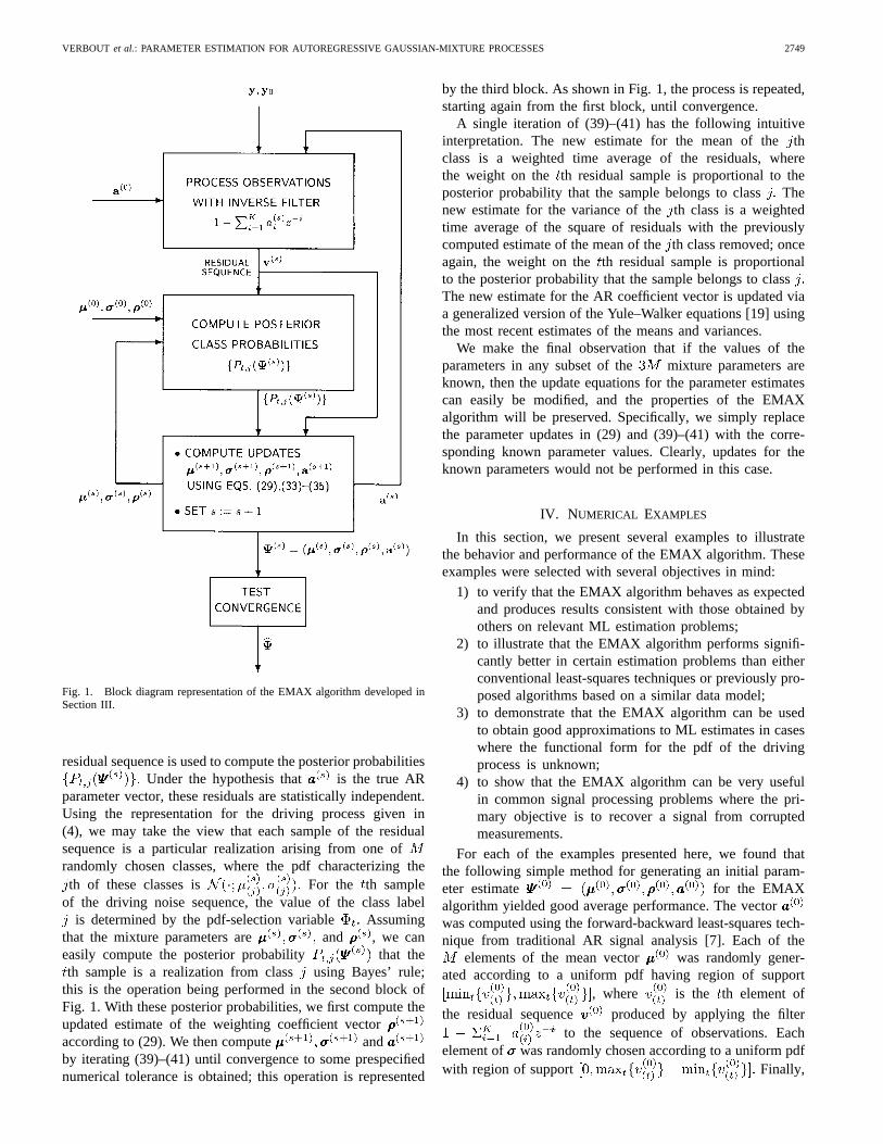
As shown in Fig. 1, the EMAX algorithm can be concep-tually decomposed into three main steps, which are iteratedto produce the final parameter estimates. Observe that thefilter can be interpreted as the currentestimate of the inverse of the AR filter. In the first blockof Fig. 1, this inverse filter is applied to the observationsto produce the residual sequence , whichcan be interpreted as an estimate of the driving noise. This
VERBOUT et al.: PARAMETER ESTIMATION FOR AUTOREGRESSIVE GAUSSIAN-MIXTURE PROCESSES 2749
Fig. 1. Block diagram representation of the EMAX algorithm developed inSection III.
residual sequence is used to compute the posterior probabilitiesUnder the hypothesis that is the true AR
parameter vector, these residuals are statistically independent.Using the representation for the driving process given in(4), we may take the view that each sample of the residualsequence is a particular realization arising from one ofrandomly chosen classes, where the pdf characterizing theth of these classes is For the th sample
of the driving noise sequence, the value of the class labelis determined by the pdf-selection variable Assuming
that the mixture parameters are and , we caneasily compute the posterior probability that theth sample is a realization from classusing Bayes’ rule;
this is the operation being performed in the second block ofFig. 1. With these posterior probabilities, we first compute theupdated estimate of the weighting coefficient vectoraccording to (29). We then compute andby iterating (39)–(41) until convergence to some prespecifiednumerical tolerance is obtained; this operation is represented
by the third block. As shown in Fig. 1, the process is repeated,starting again from the first block, until convergence.
A single iteration of (39)–(41) has the following intuitiveinterpretation. The new estimate for the mean of thethclass is a weighted time average of the residuals, wherethe weight on the th residual sample is proportional to theposterior probability that the sample belongs to classThenew estimate for the variance of theth class is a weightedtime average of the square of residuals with the previouslycomputed estimate of the mean of theth class removed; onceagain, the weight on theth residual sample is proportionalto the posterior probability that the sample belongs to classThe new estimate for the AR coefficient vector is updated viaa generalized version of the Yule–Walker equations [19] usingthe most recent estimates of the means and variances.
We make the final observation that if the values of theparameters in any subset of the mixture parameters areknown, then the update equations for the parameter estimatescan easily be modified, and the properties of the EMAXalgorithm will be preserved. Specifically, we simply replacethe parameter updates in (29) and (39)–(41) with the corre-sponding known parameter values. Clearly, updates for theknown parameters would not be performed in this case.
IV. NUMERICAL EXAMPLES
In this section, we present several examples to illustratethe behavior and performance of the EMAX algorithm. Theseexamples were selected with several objectives in mind:
1) to verify that the EMAX algorithm behaves as expectedand produces results consistent with those obtained byothers on relevant ML estimation problems;
2) to illustrate that the EMAX algorithm performs signifi-cantly better in certain estimation problems than eitherconventional least-squares techniques or previously pro-posed algorithms based on a similar data model;
3) to demonstrate that the EMAX algorithm can be usedto obtain good approximations to ML estimates in caseswhere the functional form for the pdf of the drivingprocess is unknown;
4) to show that the EMAX algorithm can be very usefulin common signal processing problems where the pri-mary objective is to recover a signal from corruptedmeasurements.
For each of the examples presented here, we found thatthe following simple method for generating an initial param-eter estimate for the EMAXalgorithm yielded good average performance. The vectorwas computed using the forward-backward least-squares tech-nique from traditional AR signal analysis [7]. Each of the
elements of the mean vector was randomly gener-ated according to a uniform pdf having region of support
, where is the th element of
the residual sequence produced by applying the filterto the sequence of observations. Each
element of was randomly chosen according to a uniform pdfwith region of support Finally,

2750 IEEE TRANSACTIONS ON SIGNAL PROCESSING, VOL. 46, NO. 10, OCTOBER 1998
TABLE ISAMPLE MEANS AND VARIANCES FOR PARAMETER ESTIMATES FROM EXAMPLE 1. ENTRIES WERE COMPUTED USING RESULTS OF5000 TRIALS
FOR i) THE ALGORITHM OF SENGUPTA AND KAY (S-K), ii) THE EMAX A LGORITHM WITH KNOWN STANDARD DEVIATIONS (EMAX-KSD),AND iii) THE EMAX A LGORITHM WITH UNKNOWN STANDARD DEVIATIONS (EMAX-USD). CRAMER–RAO BOUNDS ON THE ESTIMATION
VARIANCES, AS REPORTED BY SENGUPTA AND KAY, ARE ALSO LISTED FOR THE CASE OF KNOWN STANDARD DEVIATIONS (KSD’s)
the elements of the weighting coefficient vector were allset equal to For special cases in which certain elementsof were assumed known, no initial estimate needed to bechosen.
A. Example 1—Comparison with Previous Work (Part I)
We begin with a simple example for which numericalresults have already been reported by Sengupta and Kay [16].For direct comparison of the performance of our EMAXalgorithm to that of the Sengupta–Kay (S-K) algorithm, wehave replicated the computer simulations carried out in theirprevious work. The problem considered by those authors wasthe ML estimation of the parameters of a fourth-order ARprocess, whose AR coefficients are given by
(42)
The driving noise for this process was assumed to consistof i.i.d. samples distributed according to the two-componentGaussian-mixture pdf
(43)
where the mixture parameters and aredefined by
(44)
(45)
A plot of the power spectral density of this process is shownin Fig. 2.
Sengupta and Kay assumed that the values ofand were known and that the values of the remaining modelparameters and (and, of course, since
) were unknown. They developed a Newton–Raphsonalgorithm for obtaining ML estimates of the AR parametersand of the overall variance associated with the drivingprocess, which is given by
(46)
Obtaining an ML estimate of is, in this case, equivalentto obtaining an unconstrained ML estimate of This istrue because the parameters and stand in one-to-one correspondence, and the ML estimation procedure isinvariant with respect to such invertible transformations onthe parameters of the log-likelihood function [12].
Fig. 2. Power spectral density of fourth-order AR process discussed inExample 1.
As was done in [16], we performed a total of 5000 trials.On each trial, a sequence of 1000 data points was generatedand processed using the EMAX algorithm. The sample meansand variances of the parameter estimates produced by theEMAX algorithm are presented in Table I in the columnlabeled EMAX-KSD (where KSD stands forknown standarddeviations). The results of a separate simulation in which thestandard deviations were assumed to be unknown are alsolisted in Table I in the column labeled EMAX USD (whereUSD stands forunknown standard deviations). Remarkably,the sample variance of the estimates of the AR coefficients in-creased negligibly for the case in which the standard deviationswere unknown. However, the sample variance of the estimateof the remaining parameter increased dramatically over thatfor the case in which the standard deviations were known.
We observe from Table I that the estimate ofproduced bythe EMAX-KSD algorithm has less bias and a smaller samplevariance than the corresponding estimate produced by the S-Kalgorithm. A possible explanation for this discrepancy is thatSengupta and Kay did not constrain their estimate of(which is a function of , whereas the EMAX algorithmappropriately constrains its estimate ofto be between 0 and1. We make two further observations from Table I: i) All ofthe sample means associated with the AR parameter estimatesgenerated by the S-K algorithm exhibit slightly more bias thanthe sample means generated by the EMAX algorithm; ii) all

VERBOUT et al.: PARAMETER ESTIMATION FOR AUTOREGRESSIVE GAUSSIAN-MIXTURE PROCESSES 2751
of the sample variances of these same estimates generated bythe S-K algorithm are below the Cramer–Rao bound, whereasonly one of the sample variances generated by the EMAXalgorithm has this property. These discrepancies may stemfrom the methodology used by Sengupta and Kay. They reportthat in approximately 1% of the trials performed for thisexperiment (i.e., in approximately 50 out of 5000 trials), theirNewton–Raphson optimization algorithm did not converge.Whenever convergence was not obtained, the results of thecorresponding trial were discarded; hence, these trials are notreflected in the statistics presented in Table I. In contrast,the EMAX algorithm converged in all of the 5000 trials;hence, the results of all trials are represented in the table.The reduction in variance realized by the S-K algorithm overthe EMAX algorithm may be due to the discarded trials.This conjecture is plausible if, on those occasions whenthe Newton–Raphson algorithm did not converge, the MLparameter estimates were relatively far from the true parametervalues. If such a correlation exists between events, then it isprecisely the estimates that are never obtained because of lackof convergence that distort the sample variances reported bySengupta and Kay.
B. Example 2—Comparison with Previous Work (Part II)
Our next example illustrates that the EMAX algorithmperforms significantly better in certain kinds of estimationproblems than the algorithm previously proposed by Zhaoet al. [19], which is based on precisely the same statisticalmodel for the observed data as that presented in Section II-B. The algorithm of Zhao, which is apparently not motivatedin any respect by the EM principle, is similiar in structureto the EMAX algorithm. In particular, both of these iterativealgorithms use the same set of generalized normal equationsto solve for the estimates of the AR parameters when giventhe values of the mixture parameters. In addition, at the begin-ning of each iteration, both algorithms use the resulting ARparameter estimates to inverse filter the observation sequence.The main difference lies in the stage of each algorithm thatestimates the pdf mixture parameters from the sequence ofresiduals. As discussed in Section III, the EMAX algorithmuses the information available in the residual sequence toclimb the likelihood surface. In contrast, Zhao abandonsa likelihood-based approach (citing a desire to avoid thedegenerate solutions mentioned earlier) in favor of a heuristicclustering algorithm.
In the two-component mixture case, the clustering algorithmfirst sorts the residual samples in ascending order and thenseeks out the best point at which to divide these sortedsamples into two disjoint sets. The optimum point is definedas that which minimizes the average value of the samplevariances associated with these two sets. Once this optimumpoint is found, Zhao’s estimates of the means and variancesof the constituent Gaussians are the sample means and samplevariances associated with the two sets, and the estimate ofthe unknown weighting coefficient is simply the fraction ofsamples contained in the first set with respect to the totalnumber of residual samples.
Fig. 3. Power spectral density of fourth-order AR process discussed inExample 2.
We have observed that the algorithm of Zhao does notperform well when the constituent Gaussian densities in thedriving-noise pdf have equal means. In this example, wedemonstrate that in such a case, the performance of the EMAXalgorithm is markedly superior to that of the Zhao algorithm.In particular, we considered the problem of estimating theparameters of an ARGMIX process whose AR coefficientsare given by
(47)The pdf for the driving noise in this case was assumed to be atwo-component Gaussian-mixture pdf as in (43) but now withmixture parameters defined by
(48)
(49)
A plot of the power spectral density of this process is shownin Fig. 3.
To compare the performance of the two algorithms, weperformed a total of 500 trials. During each trial, a sequence of1000 data points was generated and processed with the EMAXalgorithm and Zhao algorithm. The sample means, variances,and mean square errors of the parameter estimates producedby the two algorithms are presented in Table II. We note thatthe Zhao algorithm produces strongly biased estimates in thisexample. In addition, we note that the mean square errorsassociated with the EMAX algorithm are approximately 25times smaller than those associated with the Zhao algorithm.Clearly, contributions to the mean square error for Zhao’sestimates come not only from the bias term but also fromthe high variance associated with her estimator.
The difficulties with the Zhao algorithm in this case maybe explained by its inability to obtain good mixture parameterestimates. The quality of the mixture parameter estimates isinherently limited because the clustering algorithm essentiallyassigns the individual densities in the Gaussian mixture tobe representatives of disjoint portions of the histogram of the

2752 IEEE TRANSACTIONS ON SIGNAL PROCESSING, VOL. 46, NO. 10, OCTOBER 1998
TABLE IISAMPLE MEANS, VARIANCES, AND MEAN SQUARE ERROR (MSE) VALUES FOR PARAMETER ESTIMATES OF EXAMPLE 2. ENTRIES WERE COMPUTED USING RESULTS OF
500 TRIALS FOR i) THE ZHAO ALGORITHM AND ii) THE EMAX A LGORITHM. RATIOS OF SAMPLE MSE VALUES (MSE OF ZHAO TO MSE OF EMAX) A RE ALSO GIVEN
(a)
(b)
Fig. 4. True marginal pdf (dashed curve) for driving process of Example 2and typical estimates of the pdf (solid curves) produced by (a) the algorithm ofZhaoet al. (20 estimates overlaid) and (b) the EMAX algorithm (20 estimatesoverlaid).
residual sequence. Thus, one of the most readily observableproblems with the approach, as illustrated in Fig. 4(a), isthat all of the estimated means of the constituent densitiesare necessarily distinct, even when the means of the truedensities are identical. Fig. 4(a) shows the true marginal pdffor the driving noise as well as typical estimates of this pdfproduced by the Zhao algorithm on separate trials. Observefrom the figure that, for about half of the trials, the pdfestimate produced by the Zhao algorithm is off center to thepositive side of zero, and for the other half, it is off centerto the negative side. On each trial, the estimated Gaussian-mixture pdf is dominated by a single component that attemptsto model most of the histogram of the residual samples.However, the resulting overall estimate is always off centerbecause the smaller of the two components in the mixtureattempts to model the remaining outliers, which are eithermuch greater or much less than zero. In contrast, as shownin Fig. 4(b), the EMAX algorithm produces pdf estimates thatbetter approximate the true driving-noise pdf.
C. Example 3—AR Process with Laplacian Driving Noise
In many applications, we would like to obtain ML estimatesfor the parameters of an AR system, but the ML problem isill-posed because the marginal pdf characterizing the drivingnoise is unknown. In certain cases, however, it may be
Fig. 5. Power spectral density of fifth-order AR process discussed in Ex-ample 3.
reasonable to assume that the true marginal pdf is accuratelymodeled by a Gaussian-mixture pdf, provided that the means,standard deviations, and weighting coefficients defining themixture are chosen appropriately. In these cases, if we processour observations with the EMAX algorithm, then we mightexpect the EMAX algorithm to find the mixture parametersthat yield a good approximation to the true driving-noise pdfand simultaneously to produce good approximations to the MLestimates for the AR parameters. With the present example, wedemonstrate the validity of this approximate approach to theML estimation problem.
In particular, we consider the parameter estimation problemfor a fifth-order AR process whose AR coefficients are givenby
(50)The driving noise for this process consists of i.i.d. samplesdistributed according to a Laplacian pdf defined by
(51)
where the scale parameter(which is related to the standarddeviation for this density by was put atA plot of the power spectral density of this process is shownin Fig. 5.
It will be interesting to compare the performance of theEMAX algorithm with that of the exact ML estimates, whichcan be computed in this case. It can be shown [2] that if

VERBOUT et al.: PARAMETER ESTIMATION FOR AUTOREGRESSIVE GAUSSIAN-MIXTURE PROCESSES 2753
TABLE IIISAMPLE MEANS AND SAMPLE MEAN SQUARE ERROR (MSE) VALUES FOR PARAMETER ESTIMATES OF EXAMPLE 3. ENTRIES
WERE COMPUTED USING RESULTS OF 500 TRIALS FOR i) THE STANDARD FORWARD-BACKWARD LEAST-SQUARES (LS)METHOD, ii) THE EMAX A LGORITHM, AND iii) THE ML ESTIMATION ALGORITHM DEVELOPED BY SCHLOSSMACHER
the samples of the driving noise for an AR process are i.i.d.and Laplacian, then the ML estimate for the AR parametervector is given by the value of that minimizes the sum ofabsolute residuals An algorithm for findingsuch a value for was proposed by Schlossmacher [15]; thisalgorithm is based on the method of iteratively reweightedleast squares and is therefore easy to implement on a computer.
To find parameter estimates for this problem with theEMAX algorithm, we fixed the number of Gaussian densitiesin the mixture at and constrained the means ofthese constituent densities to be zero. We performed a totalof 500 trials. On each trial, a sequence of 1000 data pointswas generated and processed with the EMAX algorithm. Thesample means and sample mean square errors of the parameterestimates produced by the EMAX algorithm are presented inTable III.
A summary of the sample means and sample mean squareerrors of the AR parameter estimates given by two otheralgorithms is also shown in Table III: i) the forward-backwardleast-squares method and ii) the ML algorithm of Schloss-macher. Experimental results shown in Table III confirm ourexpectation that the ML-based estimator would perform betterthan the EMAX and least-squares methods since it directlyexploits the fact that the driving noise is i.i.d. with a Laplaciandistribution. Observe from the table that the ratio of the meansquare error of the least-squares estimate to that of the MLestimate ranges approximately from 1.9–2.1. The ratio of themean square error of the EMAX estimate to that of the MLestimate ranges approximately from 1.1–1.2. Thus, in this case,the EMAX algorithm produces estimates that are much closerto the exact ML estimates than the least-squares estimates.
The superior performance of the EMAX algorithm may beattributed to the ability of its assumed Gaussian-mixture pdfto closely approximate the Laplacian pdf, as is shown for atypical case in Fig. 6(a). It is clear from this figure that theapproximation is very good over the region in which mostof the samples of the driving noise reside. However, sincethe number of Gaussian densities in the mixture is finite, anaccurate model for the Laplacian density may be obtained onlyover a finite region of support. Eventually, the tails of theGaussian-mixture pdf become bounded by a function of theform for appropriately chosen constantsand Indeed, Fig. 6(b) reveals this phenomenon with theaid of a log-magnitude scale.
It is interesting to note that although little was initiallyassumed here about the shape of the driving-noise pdf, the
(a)
(b)
Fig. 6. True Laplacian marginal pdf (dashed curve) for driving process ofExample 3 and a typical estimate of the pdf (solid curve) produced by theEMAX algorithm, plotted using (a) linear-magnitude scale (with horizontalaxis spanning�3 standard deviations) and (b) log-magnitude scale (withhorizontal axis spanning�15 standard deviations).
EMAX algorithm is also useful in a commonly encounteredvariation on this example—namely, in the case where thefunctional form of the pdf is preciselyknown except for ascale factor. Suppose, for such a case, that ML estimationis extremely difficult (possibly because of the complicatedform of the pdf) and, furthermore, that a simple Gaussianassumption leads to unacceptably poor results. In this scenario,the EMAX algorithm may once again provide a convenientway of obtaining a good approximation to the ML solution.To see this, suppose that the true pdf for the driving noisebelongs to a parameterized family of pdf’s that is invariantwith respect to scale (i.e., if the pdf for the random variable
is in the family, then the pdf for is also in the familyfor any positive scalar). For example, the Laplacian familyused in the foregoing computer simulations is scale-invariant,as is the Gaussian family and, hence, the Gaussian-mixturefamily for any fixed number of mixture components. Sincethe functional form for the true family of pdf’s is assumedknown, a good approximation for a particular pdf in thisfamily, using a Gaussian-mixture model, can be designedoffline before any data are observed. Once such a Gaussian-mixture approximation is designed, the means and standard

2754 IEEE TRANSACTIONS ON SIGNAL PROCESSING, VOL. 46, NO. 10, OCTOBER 1998
deviations of the mixture components are fixed relative to eachother. Moreover, an approximation for any other pdf in theparameterized family can easily be generated from the originalapproximation by appropriately scaling the means and standarddeviations in the Gaussian mixture. The EMAX algorithm canbe configured, through a straightforward modification of theoriginal updating formulas, to operate under such a restrictionso that it generates approximate joint ML estimates for theAR parameters and for the scale factor associated with thedriving-noise pdf.
D. Example 4—Blind Equalization in Digital Communications
Our final example is an application in digital commu-nications that has been adapted from [12]. In this exam-ple, we demonstrate that the EMAX algorithm can be usedsuccessfully in problems where the primary goal is signalreconstruction, rather than parameter estimation. In particular,we consider a communication system that uses amplitude-shiftkeying (ASK). In this scheme, the transmitter communicateswith the receiver using an -symbol alphabet ,whose elements we take to be real numbers. To send thethsymbol of a particular message sequence to the receiver,the transmitter generates a pulse (having fixed shape) and mod-ulates this pulse with the amplitude The pulse then propa-gates through the communication medium, which we assume iswell modeled by an LTI system. Finally, the receiver processesthe waveform with a linear filter to facilitate estimation of
If this filtered waveform is sampled at a rate of one sampleper symbol, then the overall communication system, i.e., thetransmitter, the medium, and the receiver, can be representedwith an equivalent discrete-time LTI system, which we refer toas the discrete-time channel. In this case, the sampled outputis the convolution of the transmitted symbol sequenceand the impulse response that characterizes the discrete-time channel. If the impulse response is anything but ashifted and scaled unit impulse, then each sample of the outputsequence will contain contributions from more than one inputsymbol, i.e., there will be intersymbol interference (ISI). If thecharacteristics of the medium are known, then the discrete-timechannel is also known, and the receiver can compensate forthe ISI using a linear filter; this technique is known as linearequalization. Often, however, the characteristics of the mediumare unknown, and the impulse response of the discrete-timechannel must first be estimated in order to compensate for theISI. One approach for accomplishing this is for the transmitterto send through the medium a training sequence that is knownto the receiver. The receiver can then identify the impulseresponse of the discrete-time channel from the output sequenceand apply the corresponding inverse filter. However, if themedium is rapidly changing, then this procedure must beperformed frequently, and the effective data rate will besubstantially reduced. An alternative approach is to performblind equalization, i.e., to estimate the impulse response ofthe discrete-time channel from the outputwithout knowingthe input, and then apply the appropriate inverse filter.
We consider a scenario in which blind equalization mustbe performed by the receiver. We assume an ASK mod-
(a)
(b)
(c)
(d)
(e)
Fig. 7. Illustration of channel equalization considered in Example 4. (a)Original symbol sequence. (b) Received sequence. (c) Restored sequenceusing standard forward-backward least-squares method. (d) Restored sequenceusing fourth-order cumulant-based Giannakis–Mendel algorithm. (e) Restoredsequence using EMAX algorithm assuming four-component Gaussian-mixturepdf.
ulation scheme that uses the four-symbol alphabetA typical 200-point input sequence to the
discrete-time channel, which was generated randomly usingthe alphabet , is shown in Fig. 7(a). We assume that thediscrete-time channel has a finite impulse response with
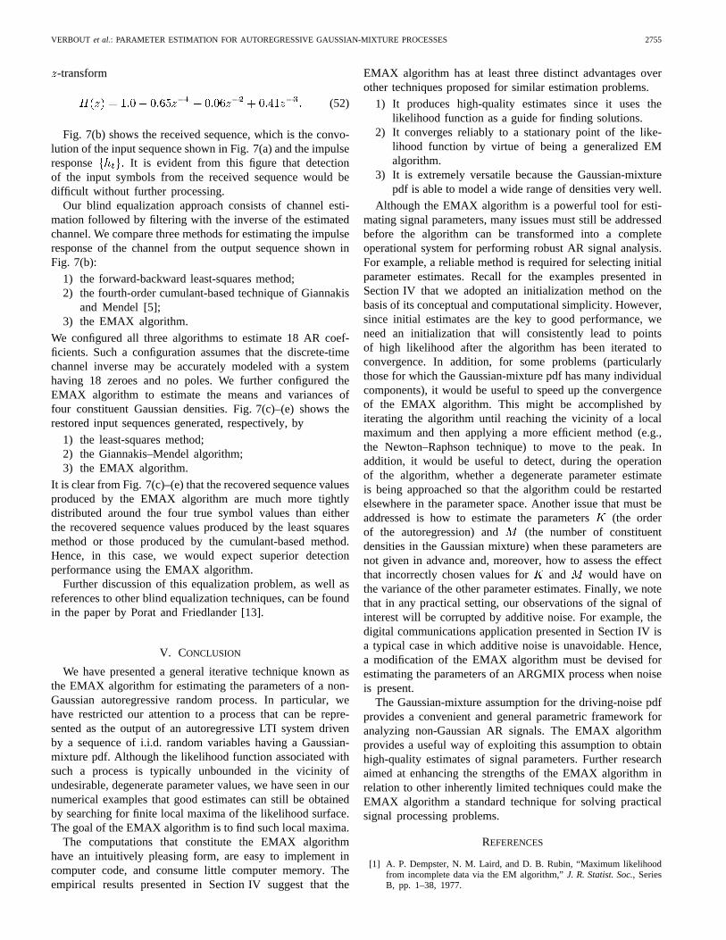
VERBOUT et al.: PARAMETER ESTIMATION FOR AUTOREGRESSIVE GAUSSIAN-MIXTURE PROCESSES 2755
-transform
(52)
Fig. 7(b) shows the received sequence, which is the convo-lution of the input sequence shown in Fig. 7(a) and the impulseresponse It is evident from this figure that detectionof the input symbols from the received sequence would bedifficult without further processing.
Our blind equalization approach consists of channel esti-mation followed by filtering with the inverse of the estimatedchannel. We compare three methods for estimating the impulseresponse of the channel from the output sequence shown inFig. 7(b):
1) the forward-backward least-squares method;2) the fourth-order cumulant-based technique of Giannakis
and Mendel [5];3) the EMAX algorithm.
We configured all three algorithms to estimate 18 AR coef-ficients. Such a configuration assumes that the discrete-timechannel inverse may be accurately modeled with a systemhaving 18 zeroes and no poles. We further configured theEMAX algorithm to estimate the means and variances offour constituent Gaussian densities. Fig. 7(c)–(e) shows therestored input sequences generated, respectively, by
1) the least-squares method;2) the Giannakis–Mendel algorithm;3) the EMAX algorithm.
It is clear from Fig. 7(c)–(e) that the recovered sequence valuesproduced by the EMAX algorithm are much more tightlydistributed around the four true symbol values than eitherthe recovered sequence values produced by the least squaresmethod or those produced by the cumulant-based method.Hence, in this case, we would expect superior detectionperformance using the EMAX algorithm.
Further discussion of this equalization problem, as well asreferences to other blind equalization techniques, can be foundin the paper by Porat and Friedlander [13].
V. CONCLUSION
We have presented a general iterative technique known asthe EMAX algorithm for estimating the parameters of a non-Gaussian autoregressive random process. In particular, wehave restricted our attention to a process that can be repre-sented as the output of an autoregressive LTI system drivenby a sequence of i.i.d. random variables having a Gaussian-mixture pdf. Although the likelihood function associated withsuch a process is typically unbounded in the vicinity ofundesirable, degenerate parameter values, we have seen in ournumerical examples that good estimates can still be obtainedby searching for finite local maxima of the likelihood surface.The goal of the EMAX algorithm is to find such local maxima.
The computations that constitute the EMAX algorithmhave an intuitively pleasing form, are easy to implement incomputer code, and consume little computer memory. Theempirical results presented in Section IV suggest that the
EMAX algorithm has at least three distinct advantages overother techniques proposed for similar estimation problems.
1) It produces high-quality estimates since it uses thelikelihood function as a guide for finding solutions.
2) It converges reliably to a stationary point of the like-lihood function by virtue of being a generalized EMalgorithm.
3) It is extremely versatile because the Gaussian-mixturepdf is able to model a wide range of densities very well.
Although the EMAX algorithm is a powerful tool for esti-mating signal parameters, many issues must still be addressedbefore the algorithm can be transformed into a completeoperational system for performing robust AR signal analysis.For example, a reliable method is required for selecting initialparameter estimates. Recall for the examples presented inSection IV that we adopted an initialization method on thebasis of its conceptual and computational simplicity. However,since initial estimates are the key to good performance, weneed an initialization that will consistently lead to pointsof high likelihood after the algorithm has been iterated toconvergence. In addition, for some problems (particularlythose for which the Gaussian-mixture pdf has many individualcomponents), it would be useful to speed up the convergenceof the EMAX algorithm. This might be accomplished byiterating the algorithm until reaching the vicinity of a localmaximum and then applying a more efficient method (e.g.,the Newton–Raphson technique) to move to the peak. Inaddition, it would be useful to detect, during the operationof the algorithm, whether a degenerate parameter estimateis being approached so that the algorithm could be restartedelsewhere in the parameter space. Another issue that must beaddressed is how to estimate the parameters(the orderof the autoregression) and (the number of constituentdensities in the Gaussian mixture) when these parameters arenot given in advance and, moreover, how to assess the effectthat incorrectly chosen values for and would have onthe variance of the other parameter estimates. Finally, we notethat in any practical setting, our observations of the signal ofinterest will be corrupted by additive noise. For example, thedigital communications application presented in Section IV isa typical case in which additive noise is unavoidable. Hence,a modification of the EMAX algorithm must be devised forestimating the parameters of an ARGMIX process when noiseis present.
The Gaussian-mixture assumption for the driving-noise pdfprovides a convenient and general parametric framework foranalyzing non-Gaussian AR signals. The EMAX algorithmprovides a useful way of exploiting this assumption to obtainhigh-quality estimates of signal parameters. Further researchaimed at enhancing the strengths of the EMAX algorithm inrelation to other inherently limited techniques could make theEMAX algorithm a standard technique for solving practicalsignal processing problems.
REFERENCES
[1] A. P. Dempster, N. M. Laird, and D. B. Rubin, “Maximum likelihoodfrom incomplete data via the EM algorithm,”J. R. Statist. Soc., SeriesB, pp. 1–38, 1977.

2756 IEEE TRANSACTIONS ON SIGNAL PROCESSING, VOL. 46, NO. 10, OCTOBER 1998
[2] N. R. Draper and H. Smith,Applied Regression Analysis. New York:Wiley, 1950.
[3] R. O. Duda and P. E. Hart,Pattern Classification and Scene Analysis.New York: Wiley, 1973.
[4] B. S. Everitt and D. J. Hand,Finite Mixture Distributions. London,U.K.: Chapman and Hall, 1981.
[5] G. B. Giannakis and J. M. Mendel, “Identification of nonminimum phasesystems using higher order statistics,”IEEE Trans. Acoust., Speech,Signal Processing, vol. 37, pp. 360–377, Mar. 1989.
[6] D. G. Luenberger,Linear and Nonlinear Programming, 2nd ed. Read-ing, MA: Addison Wesley, 1984.
[7] S. L. Marple,Digital Spectral Analysis with Applications. EnglewoodCliffs, NJ: Prentice-Hall, 1987.
[8] G. J. McLachlan and K. E. Basford,Mixture Models. New York:Marcel Dekker, 1988.
[9] J. M. Mendel, “Tutorial on higher-order statistics (spectra) in signal pro-cessing and system theory: Theoretical results and some applications,”Proc. IEEE, vol. 79, Mar. 1991.
[10] C. L. Nikias and M. R. Raghuveer, “Bispectrum estimation: A digitalsignal processing framework,”Proc. IEEE, vol. 75, pp. 869–891, July1987.
[11] C. L. Nikias and A. P. Petropulu,Higher-Order Spectra Analysis:A Nonlinear Signal Processing Framework. Englewood Cliffs, NJ:Prentice-Hall, 1993.
[12] B. Porat,Digital Processing of Random Signals: Theory and Methods.Englewood Cliffs, NJ: Prentice-Hall, 1994.
[13] B. Porat and B. Friedlander, “Blind equalization of digital communica-tion channels using high-order moments,”IEEE Trans. Signal Process-ing, vol. 39, pp. 522–526, Feb. 1991.
[14] R. A. Redner and H. F. Walker, “Mixture densities, maximum likelihoodand the EM algorithm,”SIAM Rev., vol. 26, no. 2, Apr. 1984.
[15] E. J. Schlossmacher, “An interactive technique for absolute deviationscurve fitting,” J. Amer. Statist. Assoc., vol. 68, no. 344, Dec. 1973.
[16] D. Sengupta and S. Kay, “Efficient estimation of parameters for non-Gaussian autoregressive processes,”IEEE Trans. Acoust., Speech, SignalProcessing, vol. 37, June 1989.
[17] D. M. Titterington, A. F. M. Smith, and U. E. Makov,Statistical Analysisof Finite Mixture Distributions. Chichester, U.K.: Wiley, 1985.
[18] C. F. J. Wu, “On the convergence properties of the EM algorithm,”Ann.Statist., vol. 11, no. 1, pp. 95–103, 1983.
[19] Y. Zhao, X. Zhuang, and S.-J. Ting, “Gaussian mixture density modelingof non-Gaussian source for autoregressive process,”IEEE Trans. SignalProcessing, vol. 43, Apr. 1995.
Shawn M. Verbout received the B.S. degree inmathematics from Illinois State University, Normal,in 1987 and the S.M. degree in electrical engineer-ing from the Massachusetts Institute of Technology(MIT), Cambridge, in 1994. He is currently pursuingthe Ph.D. degree in electrical engineering at MIT.
Since 1987, he has been with MIT Lincoln Lab-oratory, Lexington, where he has worked primarilyon problems in automatic detection and recognitionof remotely sensed objects. Since 1992, he has beenaffiliated with the Digital Signal Processing Group
in the Research Laboratory of Electronics, MIT. His current research interestsare in the general area of statistical signal processing with particular emphasison problems involving non-Gaussian signals.
James M. Ooi was born in Singapore in 1970.He received the S.B., S.M., and Ph.D. degreesin electrical engineering from the MassachusettsInstitute of Technology (MIT), Cambridge, in 1992,1993, and 1997, respectively. From 1995 to 1997, heheld an AT&T Bell Laboratories Ph.D. Fellowship.
From 1993 to 1997, he was with the DigitalSignal Processing Group at MIT. During the sameperiod, he was a teaching assistant for classes incomputer programming, digital signal processing,and statistical signal processing. He has been on
the technical staff at the Texas Instruments Computer Science Center, from1989 to 1992, Orbital Sciences Corporation in 1993, and AT&T/LucentTechnologies Bell Laboratories from 1995 to 1996, where he has researched avariety of topics including computer vision, speech and audio coding, satellitecommunication, and error-correcting codes. He is currently a consultantwith the Mitchell Madison Group, Cambridge, MA, a strategic managementconsulting firm. His current interests include information theory, fuzzy logic,game theory, and estimation.
Jeffrey T. Ludwig received the S.B. degree in aero-nautics and astronautics in 1991, the S.M. degree inelectrical engineering and computer science in 1993,and the Ph.D. degree in electrical engineering andcomputer science in 1997, all from the Massachu-setts Institute of Technology (MIT), Cambridge.
He has served as a teaching assistant for graduateand undergraduate classes at MIT in digital signalprocessing, feedback systems, and control theory,has authored more than a dozen technical publica-tions, and holds one U.S. patent. He has five years
experience as a principal engineer with Hughes Electronics Corporation, twoyears experience as a research assistant at the MIT Lincoln Laboratory, andone year experience as a research associate with the Signal Processing Centerof Technology, Lockheed Martin Corporation. He recently joined DelphiStructured Finance Corporation, where he has focused on the developmentand marketing of leading edge loan portfolio analytics and cash managementsystems for the securitization industry.
Alan V. Oppenheim (F’77) received the S.B. andS.M. degrees in 1961 and the Sc.D. degree in 1964,all in electrical engineering, from the MassachusettsInstitute of Technology (MIT), Cambridge. He wasalso the recipient of an honorary doctorate from TelAviv University, Tel-Aviv, Israel, in 1995.
In 1964, he joined the faculty at MIT, where heis currently the Ford Professor of Engineering anda MacVicar Faculty Fellow. Since 1967, he has alsobeen affiliated with MIT Lincoln Laboratory andsince 1977 with the Woods Hole Oceanographic
Institution. His research interests are in the general area of signal processingand its applications. He is coauthor of the widely used textbooksDiscrete-Time Signal ProcessingandSignals and Systems. He is also editor of severaladvanced books on signal processing.