1

GPU-Accelerated Minimum Distance and ClearanceQueries

Adarsh Krishnamurthy, Sara McMains, Kirk Haller

Abstract—We present practical algorithms for accelerating distance queries on models made of trimmed NURBS surfaces using programmableGraphics Processing Units (GPUs). We provide a generalized framework for using GPUs as co-processors in accelerating CAD operations. Bysupplementing surface data with a surface bounding-box hierarchy on the GPU, we answer distance queries such as finding the closest point ona curved NURBS surface given any point in space and evaluating the clearance between two solid models constructed using multiple NURBSsurfaces. We simultaneously output the parameter values corresponding to the solution of these queries along with the model space values.Though our algorithms make use of the programmable fragment processor, the accuracy is based on the model space precision, unlike earliergraphics algorithms that were based only on image space precision. In addition, we provide theoretical bounds for both the computed minimumdistance values as well as the location of the closest point. Our algorithms are at least an order of magnitude faster and about two orders ofmagnitude more accurate than the commercial solid modeling kernel ACIS.

Index Terms—Minimum Distance, Closest Point, Clearance Analysis, NURBS, GPU, Hybrid CPU/GPU Algorithms

F

1 INTRODUCTION

Distance queries such as finding the minimum distance to asurface play an important role in many computer aided designand analysis applications, including tolerancing, clearanceanalysis, and accessibility analysis. Minimum distance queriesare especially useful while designing complex assemblies toallow for sufficient clearance between different mechanicalcomponents. Such queries are easily answered if the objects ormodels are made of planar faces and have boxy shapes. How-ever, modern designs make use of curved freeform surfaces;the standard representation of choice being Non-Uniform Ra-tional B-Spline (NURBS) surfaces. Minimum distance querieson such freeform surfaces are currently being solved bycommercial solid modeling software by first evaluating andtessellating the surface and then finding the minimum distanceto the tessellation vertices [1]. This approach, in additionto being extremely slow and computationally intensive, isdependent on the tessellation resolution for the accuracy ofthe solution; the surface has to be very finely tessellated toget the required accuracy.

A technique to accelerate such slow geometric queries isto use programmable GPUs. We have developed a unifiedframework that uses GPUs as co-processors in acceleratinggeometric computations; we make use of the fragment pro-cessor in a GPU to perform parallel parts of the computationsand use the CPU to perform the inherently serial parts.This framework can be extended to solve a wide range ofgeometric queries; we give a few practical examples of using

• A. Krishnamurthy, and S. McMains are with the Department of MechanicalEngineering, University of California, Berkeley, CA, USA.e-mail: {adarsh—mcmains}@me.berkeley.edu

• K. Haller is with SolidWorks Corporation, Concord, MA, USA.e-mail: khaller@solidworks.com

Manuscript received Jan 22, 2010, revised Jun 12, 2010

this framework to answer distance queries. Previous GPU-based algorithms that render to the screen to perform thesecomputations have restricted accuracy corresponding to thedimensions of the pixel or window. Our framework allows forthe GPU algorithms to operate in the model space; therefore,the results of these geometric queries are accurate to anyarbitrary user-defined tolerance.

Solid modeling kernels support certain distance queriessuch as the minimum distance from a point to a surface andthe minimum distance between two surfaces. Applicationsof such distance queries include: finding the closest surfacepoint on a surface to provide haptic feedback; dimensioningand tolerancing of CAD models; and constructing distancefields. In this paper, we present an algorithm that uses ourhybrid CPU/GPU framework consisting of surface bounding-boxes to accelerate these queries. We focus on performingdistance queries on objects made of trimmed NURBS surfacesin this paper. However, our algorithms are applicable for anysurface that can be supplemented with a surface bounding-boxstructure. We provide theoretical bounds on the accuracy ofboth the computed minimum distance as well as the location ofthe closest point on the surface, which allow for arbitrary user-defined tolerance values. This is especially important in CADsystems since these distances might be used by the designer todefine subsequent features; the model might fail to regenerateif there is an error in the computed distance.

In this paper, we provide a hybrid CPU/GPU framework toaccelerate minimum distance computations, which is expandedfrom our previous conference presentation [2]. Our maincontributions include:• A practical GPU algorithm to find the minimum distance

to a surface given any point in space. We use our hybridframework to compute the distances efficiently in parallelusing the GPU.

• A fast algorithm that computes the minimum distancebetween two surfaces or between two solid models rep-

2

(a) NURBS Clearance (b) Trimmed NURBS Clearance (c) Object Clearance

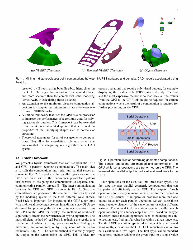
Fig. 1. Minimum distance/closest point computations between NURBS surfaces and complex CAD models accelerated usingthe GPU.

resented by B-reps, using bounding-box hierarchies onthe GPU. Our algorithm is orders of magnitude fasterand more accurate than the commercial solid modelingkernel ACIS in calculating these distances.

• An extension to the minimum distance computation al-gorithm to compute the minimum distance between twotrimmed NURBS surfaces.

• A unified framework that uses the GPU as a co-processorto improve the performance of algorithms used for solv-ing geometric queries. This framework can be extendedto accelerate several related queries that are based onproperties of the underlying shapes such as normals orcurvature.

• Theoretical guarantees for all of our geometric computa-tions. They allow for user-defined tolerance values thatare essential for integrating our algorithms in a CADsystem.

1.1 Hybrid Framework

We present a hybrid framework that can use both the CPUand GPU to perform geometric computations. The main ideais to split the computations into serial and parallel stages asshown in Fig. 2. To perform the parallel operations on theGPU, we make use of the map-reduce parallelism patternthat consists of assigning the computations to separate non-communicating parallel threads [3]. The inter-communicationbetween the CPU and GPU is shown in Fig. 3. Once thecomputations are performed, the computed result can be usedby the modeling system in the three different ways shown.Read-back is important for integrating the GPU algorithmswith traditional modeling systems. In addition, since GPUs aredesigned for pipelining the data only in one direction fromthe CPU to the GPU for display, the method of read-backsignificantly affects the performance of hybrid algorithms. Themost efficient method of read-back is reducing the results to asmaller set of values by using operations such as finding themaximum, minimum, sum, or by using non-uniform streamreductions ( [4], [5]). The second method is to directly displaythe output on the screen using the GPU. This is ideal for

certain operations that require only visual outputs; for exampledisplaying the evaluated NURBS surface directly. The lastand the most expensive method is to read back all the resultsfrom the GPU to the CPU; this might be required for certaincomputations where the result of a computation is required forfurther processing on the CPU.

Parallel Operations

Serial Operations

Serial Operations

Map

Reduce

Fig. 2. Operation flow for performing geometric computations.The parallel operations are mapped and performed on theGPU while serial operations are performed on the CPU. Theintermediate parallel output is reduced and read back to theCPU.

Our operations on the GPU fall into three main types. Thefirst type includes parallel geometric computations that canbe performed efficiently on the GPU. The outputs of suchoperations are usually numeric values that are then stored inthe GPU as textures. If an operation produces more than oneoutput value for each parallel operation, we can store thoseusing separate channels of the same texture or using differenttextures. The second GPU operation type is parallel searchoperations that give a binary output of 0 or 1 based on the typeof search; these include operations such as bounding-box in-tersection tests, finding if a value lies within a given range, etc.The third GPU operation type is reduction, which is performedusing multiple passes on the GPU. GPU reductions can in turnbe classified into two types. The first type, called standardreductions, include reducing the given input to a single value

3

Hybrid CPU/GPUTraditional

Serial

Computation

CPU GPUMap

Parallel

Computation

Reduce

Display

Read

Fig. 3. Schematic showing our hybrid framework that extendstraditional geometric computations to use the GPU as a co-processor to perform some parts of the computations in paral-lel.

such as computing the sum, min, max, etc. Standard reductionoperations are usually performed in O(log n) passes and henceare very efficient. The second type of reductions, called non-uniform stream reductions, reduces the input to a smallerset of values. Non-uniform stream reduction operations areparticularly important when the result of a reduction operationis not a single value but multiple values that satisfy a particularcriterion. Since the positions of the output elements do nothave any fixed correspondence with the positions of the input,the stream-reduction process is considered non-uniform. Wemake use of an O(n) GPU stream-reduction algorithm thatwe presented in previous work [6] to perform non-uniformstream reductions.

To perform geometric computations on NURBS surfaces orassemblies, we make use of a surface bounding-box structureto map the computations to the GPU. We make use ofAxis-Aligned Bounding-Boxes (AABBs) constructed from anevaluated mesh of points on the NURBS surface to acceleratethe computations [6]. The main advantage of AABBs overOriented Bounding-Boxes (OBBs) is that several geometriccomputations such as finding intersections and distances aresimpler in the case of AABBs. This is especially importantbecause the efficiency of GPU programs can be reduceddramatically with increases in the complexity of the parallelkernels that are used. The individual computational kernelsfor OBBs are more complex and contain many branchingconditions; the GPU has to wait until the most computationallyintensive branch of the kernel in a particular pass is completedbefore proceeding to the next pass. In addition, since OBBkernels make use of more temporary registers, the number ofcomputations that can be active simultaneously on the GPU(called fragments in flight) is reduced; it is difficult to hide thememory access latency in this case. Thus, we found that theadvantage provided by tight OBBs is offset by the increasein complexity of the algorithms that use them. We achievebetter results by using AABBs even if we must decomposethe model to a finer resolution with AABBs than OBBs inorder to maintain the same tolerance bounds.

2 BACKGROUND AND PREVIOUS WORK

2.1 Related Work

Minimum distance computations are used by many algorithmsthat generate geometrical constructs such as Voronoi diagramsand medial axis transforms. They are also used in path plan-ning and robot motion planning [7] and for projecting pointsonto a patch of a CAD model [8]. Minimum distance compu-tations on curved NURBS surface are very time-consuming;hence, the commercial solid modeling system ACIS makesuse of the tessellation of the surface to find the closest vertexor pair of vertices while performing tolerance analysis [1].Johnson et al. [9] gave a unified framework for minimumdistance computations, which was later extended to find theclosest point for haptics applications by Nelson et al. [10].We use a similar method that uses AABBs to find the regionsof the model that are likely to contain the closest points.However, the methods they describe were better suited fora serial CPU implementation, since they make use of theconvex hull of the freeform surface to iteratively refine thesearch. In our algorithm, the distance computations and searchoperations are done in parallel, which is better suited for aGPU implementation. In addition, we also provide theoreticalguarantees for the solutions we compute.

Edelsbrunner [11] proved that the minimum distance be-tween two convex polygons can be computed in O(log n).However, the algorithm used in the proof is theoretical andhas large time-constants in practice. Quinlan [12] extendedthe minimum distance computations to non-convex objectsby first performing a convex decomposition and then usingbounding spheres for the convex pieces to create a hierarchy.However, this method is not practical for dynamic geometriessince the convex decomposition might be expensive. Chen etal. [13] compute the minimum distance between a point anda NURBS curve by subdividing the curve into portions thatmight contain the closest point. Many minimum distance algo-rithms use Bounding Volume Hierarchies (BVHs) to acceleratethe computations. CPU algorithms usually make use of BVHsthat are more complex than AABBs. Gottschalk et al. [14]make use of OBBs to perform distance computations. Larsenet al. [15] perform proximity queries using a construct calleda sphere swept volume, which consists of a sphere swept overa point, line or a plane, as primitives of a BVH.

Collision detection and distance field computation are twoproblems that are closely related to minimum distance com-putations that have been effectively accelerated using theGPU. Occlusion queries on graphics hardware were used byGovindaraju et al. [16] to detect collisions of polygonal meshesin large environments. Greß et al. [17] solve the collisiondetection problem by generating a bounding-box hierarchy fordeformable parameterized surfaces and then detect collisionsby checking overlap between the bounding-boxes using theGPU. Sud et al. [18] use the GPU to generate 3D distancefields by first slicing the model into 2D slices and by usingculling and spatial coherence to reduce the number of distancecomputations in each slice. Lauterbach et al. [19] use the GPUto construct BVHs that can then be used to accelerate collisiondetection.

4

There has been only limited use of GPUs to performgeometric operations because they are restricted to image-space resolution if the computations are to be performed byrendering on the screen. Agarwal et al. [20] make use of theGPU to perform geometric computations on a stream of pointsby using point-line duality. They compute geometric propertiessuch as diameter and width of a set of points. However, thesealgorithms are not stable for points that are very close andare limited to image-space resolution. Hoff et al. [21] usethe GPU to perform fast proximity queries on 2D shapesusing a pixel grid to perform distance computations, but theirtechnique does not extend to 3D shapes. To overcome theimage-space resolution for spline intersections, researchers atSINTEF adapted the serial subdivision algorithm to use theGPU. They accelerate the computations by using the GPUto test for intersections and iteratively subdivide the splinepatches until a prescribed accuracy is attained [22], [23].

Prior algorithms for proximity queries on spline modelsused higher-order bounding volumes such as OBBs or sweptspheres. Krishnan et al. calculate contact between splinemodels using a combination of bounding volumes that includespherical shells and OBBs [24]. Even though these higher-order bounding volumes have low memory requirements, theindividual overlap computations are more complex. We makeuse of an AABB hierarchy in which the bounding boxes arenot as tight as higher-order bounding volumes, but reduce thecomplexity of the computations for each bounding-box pair.

Our algorithm to compute the minimum distance betweenobjects is an hybrid CPU/GPU algorithm that uses the CPUfor certain computations that are inherently serial. Lauterbachet al. have recently developed a GPU algorithm where thehierarchy traversal and primitive queries are also performedon the GPU [25]. Even though such an exclusive GPUalgorithm overcomes the CPU/GPU bottleneck, it requiresnewer hardware to perform the atomic operations on theGPU. However, these operations are not supported by all GPUhardware vendors; as a result, such algorithms will be difficultto be adopted by the CAD industry. Furthermore, parts of ouralgorithm that are performed on the CPU can be easily portedto the GPU when atomic operations are more widely supportedby all GPU vendors.

2.2 NURBS Evaluation and Modeling

Our minimum distance computation and silhouette extractionalgorithms build on our previous papers on GPU NURBSevaluation and modeling. We present a short outline of ouralgorithms that were explained in detail in [2], [6], [26], [27].In our NURBS evaluation paper [27] we developed a methodto directly evaluate a mesh of points on a NURBS surfaceusing the GPU. Our algorithm used a fragment program toevaluate a NURBS surface of arbitrary degree in severalpasses. After evaluation we have the sampled NURBS surfaceas 4-component vectors—(x, y, z, w) coordinates—in spacestored as a texture on the GPU. While rendering, we interpretthese values stored in the texture as vertex coordinates using aVertex Buffer Object (VBO) and display the VBO as a meshdirectly on the screen.

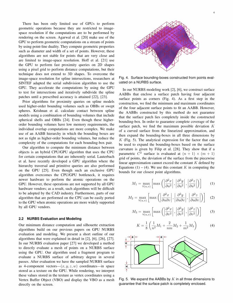
Fig. 4. Surface bounding-boxes constructed from points eval-uated on a NURBS surface.

In our NURBS modeling work [2], [6], we construct surfaceAABBs that enclose a surface patch having four adjacentsurface points as corners (Fig. 4). As a first step in theconstruction, we find the minimum and maximum coordinatesof the four adjacent surface points to fit an AABB. However,the AABBs constructed by this method do not guaranteethat the surface patch lies completely inside the constructedbounding-box. In order to guarantee complete coverage of thesurface patch, we find the maximum possible deviation Kof a curved surface from the linearized approximation, andthen expand the bounding-boxes in all three dimensions byK (Fig. 5). The analytical expression for the factor that canbe used to expand the bounding-boxes based on the surfacecurvature is given by Filip et al. [28]. They show that if aparametric C2 surface is evaluated at (n + 1) × (m + 1)grid of points, the deviation of the surface from the piecewiselinear approximation cannot exceed the constant K defined byEquations (1) – (4). We use this constant K in computing thebounds for our closest point algorithms.

M1 = max∀(u,v)

[max

(∣∣∣∣∂2x∂u2

∣∣∣∣ , ∣∣∣∣∂2y∂u2

∣∣∣∣ , ∣∣∣∣∂2z∂u2

∣∣∣∣)] (1)

M2 = max∀(u,v)

[max

(∣∣∣∣ ∂2x∂u∂v

∣∣∣∣ , ∣∣∣∣ ∂2y∂u∂v

∣∣∣∣ , ∣∣∣∣ ∂2z∂u∂v

∣∣∣∣)] (2)

M3 = max∀(u,v)

[max

(∣∣∣∣∂2x∂v2

∣∣∣∣ , ∣∣∣∣∂2y∂v2

∣∣∣∣ , ∣∣∣∣∂2z∂v2

∣∣∣∣)] (3)

K =1

8

(1

n2M1 +

2

nmM2 +

1

m2M3

)(4)

K K

KK

Fig. 5. We expand the AABBs by K in all three dimensions toguarantee that the surface patch is completely enclosed.

5

An alternative approach for constructing an AABB hi-erarchy for the NURBS surface is to recursively constructthe bounding-boxes by evaluating surface points using knotinsertion. This method has the advantage that it can be adap-tively refined based on the curvature of the surface. However,implementing this method on the GPU is tedious since thenumber of bounding-boxes in the finest level of the hierarchyis not known a priori. In addition, recursive algorithms do notachieve optimal performance when implemented on the GPU.Hence, we construct AABBs as explained above.

3 DISTANCE QUERIES ON NURBS SURFACES

We first present distance queries that are performed on indi-vidual NURBS surfaces and later in Sec. 5 extend them tocomplex objects made up of multiple curved surfaces.

3.1 Minimum Distance to a NURBS Surface

The first distance query we accelerate using the GPU iscomputing the minimum distance and the closest point on aNURBS surface given any point in space. As a first step, weevaluate the NURBS surface as a grid of points using ourNURBS evaluator and construct surface AABBs enclosingfour neighboring points. Using these bounding-boxes andthe input point, we calculate the range of distances to eachbounding box as explained in Sec. 3.2.

Fig. 6 shows how our GPU closest point algorithm fits intoour hybrid framework. We first use the GPU to compute theminimum and maximum distance to each AABB efficiently inparallel. These distances are stored using the red and greenchannels in a min/max texture on the GPU. We then performa parallel reduction in log n passes on the GPU to find thebounding-box with the minimum lower value for the distancerange. We read back the range of this particular bounding-box.In the next pass, we use the upper bound of this particularbounding-box as a distance cutoff to search for potentiallyclose bounding-boxes. We use the GPU to perform a parallelsearch on the same min/max texture we computed in the firststep to find all the bounding-boxes whose ranges overlap withthe upper bound. This prunes the list of bounding-boxes tosearch for the closest point; we read back this smaller list byperforming non-uniform stream reduction on the results of thesearch.

Once we read back the potentially close bounding-boxes,we approximate the surface patch inside each of the boundingboxes with two triangles formed from the evaluated surfacepoints. We then find the distance to each of these triangles andfinally choose the one with the minimum distance. We also findthe point lying on the triangle that has the minimum distanceas the closest point on the surface. We prove theoretical errorbounds for the evaluated minimum distance and the calculatedclosest point in Section 4.

3.2 Minimum and Maximum Distance to an AABB

The first step of our minimum distance algorithm requires thecomputation of the minimum and maximum distance betweena point and an AABB. Since we want to perform these

CP

U/G

PU

D

ata

Tra

nsfe

r

Min Reduce

Min/Max Distances

Parallel Find

Non-Uniform

Stream

Reduction

0 0

0 1

1 0

1 2

1 3

Addresses

Upper bound of

Minimum Distance

Bounding-Boxes

within Range

= Distance Range

0

Max KEY

Fig. 6. Schematic of our closest point algorithm showing theinter-communication between the CPU and GPU. The verticalbars represent the range of minimum and maximum distancesfrom the point to the bounding box.

computations in parallel for each AABB, the computationshave to be efficient and optimized for the GPU. The maximumdistance can be computed in a straightforward manner byfinding the vertex of the bounding-box that is farthest from thegiven point. However, to compute the minimum distance, wenot only need to find the minimum distance to the vertices ofthe AABB but also to the faces. The number of computationsbecomes prohibitively many if we have to check all thepossibilities.

We make use of the fact that the bounding-boxes are axis-aligned to efficiently compute the minimum and maximumdistance. This makes the calculations simpler and unified forcomputing both the minimum and maximum distance simulta-neously (Fig. 7). For computing the maximum distance froma point O to an AABB, we compute the maximum distancealong each axis separately and finally take the L2 norm of theindividual maximum distances to find the maximum distance(Equations (5) – (8)). However, if we extend the same methodto compute the minimum distance, we have to make surethat the individual distance components are non-zero; if wedirectly subtract the half bounding-box widths, we will endup with negative distances. To overcome this, we take theminimum distance along a particular direction as zero if it isnegative (Equations (9) – (12)).

xmax = Dcx +Bx (5)

ymax = Dcy +By (6)

zmax = Dcz +Bz (7)

Dmax =√

(x2max + y2max + z2max) (8)

xmin = max(Dcx −Bx, 0) (9)

ymin = max(Dcy −By, 0) (10)

zmin = max(Dcz −Bz, 0) (11)

Dmin =√(x2min + y2min + z2min) (12)

6

Dcx

2Bx

By

2By

O

DcyC

Bx

(a) Maximum Distance

Dcx

2Bx

2By

O

DcyC

Bx

By

(b) Minimum Distance

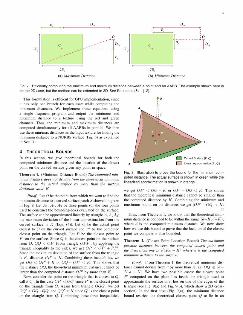
Fig. 7. Efficiently computing the maximum and minimum distance between a point and an AABB. The example shown here isfor the 2D case, but the method can be extended to 3D. See Equations (5) – (12).

This formulation is efficient for GPU implementation, sinceit has only one branch for each max while computing theminimum distances. We implement these equations usinga single fragment program and output the minimum andmaximum distance to a texture using the red and greenchannels. Thus, the minimum and maximum distances arecomputed simultaneously for all AABBs in parallel. We thenuse these min/max distances as the input texture for finding theminimum distance to a NURBS surface (Fig. 6) as explainedin Sec. 3.1.

4 THEORETICAL BOUNDS

In this section, we give theoretical bounds for both thecomputed minimum distance and the location of the closestpoint on the curved surface given any point in space.

Theorem 1. (Minimum Distance Bound) The computed min-imum distance does not deviate from the theoretical minimumdistance to the actual surface by more than the surfacedeviation value K.

Proof: Let O be the point from which we want to find theminimum distance to a curved surface patch S showed in greenin Fig. 8. Let A1, A2, A3 be three points (of the four pointsused to construct the bounding-box) evaluated on the surface.The surface can be approximated linearly by triangle A1A2A3;the maximum deviation of the linear approximation from thecurved surface is K (Eqn. (4)). Let Q be the actual pointclosest to O on the curved surface and P ′ be the computedclosest point on the triangle. Let P be the closest point toP ′ on the surface. Since Q is the closest point on the surfacefrom O, OQ < OP . From triangle OPP ′, by applying thetriangle inequality to the sides, we get OP < OP ′ + PP ′.Since the maximum deviation of the surface from the triangleis K, distance PP ′ < K. Combining these inequalities, weget OQ < OP ′ + K or OQ − OP ′ < K. This shows thatthe distance OQ, the theoretical minimum distance, cannot belarger than the computed distance OP ′ by more than K.

Now, consider the point on the triangle that is closest to Q,call it Q′. In this case OP ′ < OQ′ since P ′ is the closest pointon the triangle from O. Again from triangle OQQ′, we getOQ′ < OQ+QQ′ and QQ′ < K since Q′ is the closest pointon the triangle from Q. Combining these three inequalities,

A1

A3

PQ

P´

O

Q´

d

A2

Curved Surface (P, Q)

Linear Approximation (P', Q')

Fig. 8. Illustration to prove the bound for the minimum com-puted distance. The actual surface is shown in green while thelinearized approximation is shown in orange.

we get OP ′ < OQ + K or OP ′ − OQ < K. This showsthat the theoretical minimum distance cannot be smaller thanthe computed distance by K. Combining the minimum andmaximum bound on the distance, we get |OP ′ −OQ| < K.

Thus, from Theorem 1, we know that the theoretical mini-mum distance is bounded to lie within the range (d−K, d+K),where d is the computed minimum distance. We now showhow we use this bound to prove that the location of the closestpoint we compute is also bounded.

Theorem 2. (Closest Point Location Bound) The maximumpossible distance between the computed closest point andthe theoretical one is

√4Kd+K2 where d is the computed

minimum distance to the surface.

Proof: From Theorem 1, the theoretical minimum dis-tance cannot deviate from d by more than K, i.e. OQ ∈ [d−K, d + K]. We have two possible cases: the closest pointP ′ computed on the plane lies inside the triangle used toapproximate the surface or it lies on one of the edges of thetriangle (see Fig. 9(a) and Fig. 9(b), which show a 2D cross-section). In the first case (Fig. 9(a)), the minimum distancebound restricts the theoretical closest point Q to lie in an

7

2' 4P Q dK K

d-K d+K

Q

P´

O

2K

Curved Surface

Linear Approximation

Max Possible Deviation

Minimum Distance Bound

Linear Approximation Bound

K

2 2( ) ( )

= 4

d K d K

dK

d

(a) Case 1

d-Kd+K

O

d

QP´

(b) Case 2

Fig. 9. Illustration to evaluate the bound for the computed closest point location when the closest point on the plane lies either(a) inside or (b) on the edge of the triangle approximating the surface.

annular region between spheres with center O and radii d+Kand d − K (marked in blue). From our tessellation boundK, we know that the actual surface lies within a region ofwidth 2K centered around the approximating triangle (markedin red). Thus the point Q lies in the intersection of theseoverlapping regions. The maximum possible distance P ′Qin this intersecting region is

√4Kd+K2. In the second

case (Fig. 9(b)), the approximating triangle is oriented at anobtuse angle with respect to OP ′. In this case, the maximumdistance in the overlapping region occurs only when OP ′ isperpendicular to the triangle; for all other angles of rotation ofOP ′, it is always less than

√4Kd+K2 (please refer to the

Appendix for a detailed explanation). Hence, the maximumpossible distance between the computed closest point and thetheoretical one is always

√4Kd+K2.

Thus, both the computed minimum distance and the locationof the closest point are bounded. We show in the Resultssection that these theoretical bounds translate to realistic valuesthat are useful in practice. Next, we extend our minimumdistance computations to compute the minimum distance be-tween two NURBS surfaces or two complex CAD objectsrepresented as B-reps.

5 CLEARANCE ANALYSIS

5.1 Minimum Distance Between Two NURBS Surfaces

We use a method similar to finding the minimum distance froma point to a surface to find the minimum distance betweentwo surfaces. However, it is impractical to use this methoddirectly because the number of distance comparisons increaseas O(n2), where n is the number of AABBs of each surface.Therefore, we make use of a method that uses bounding-boxhierarchies to successively refine the number of potentially-close bounding-box pairs. We show that this approach, whichis similar to a breadth-first search, can also be fit into ourhybrid framework. We perform the search for potentially-closebounding-box pairs in parallel at each level using the GPU.

10 1

2 3

0 1

2 3

Level n

Bounding Box

Hierarchy 1

Min/Max Distances

31 33

Potentially

Close AABBs

00 01 02 03

10 11 12 13

20 21 22 23

30 31 32 33

00 01 02 03

10 11 12 13

20 21 22 23

30 31 32 33

CP

U/G

PU

Da

ta T

ran

sfe

r

Non-Uniform

Stream Reduction

Parallel Search for

Potentially Close

AABB

Refine to Next

Level3

0 1

2 3

0 1

2 3

Bounding Box

Hierarchy 2

0

2

1

3

0 1

2 3

0

2

Fig. 10. We perform minimum distance computation betweentwo NURBS surfaces with the help of AABB hierarchies forboth the surfaces. We compute a list of potentially closebounding-boxes at each level using the GPU and then refineon the CPU until we reach a set of potentially close bounding-boxes at the lowest level.

We first construct surface AABBs as shown in Fig. 4; denotethese as original AABBs. We then generate a bounding-boxhierarchy by recursively combining four AABBs in a level toget a bigger AABB of the next higher level. Thus, we constructan AABB hierarchy starting with the original AABBs andfinally reaching a single, level-0 bounding box. This operationcan be effectively performed in O(log n) passes using theGPU. We store the bounding-boxes in a manner that optimizesGPU storage space (Fig 10) similar to mip-map layouts. Whenthe model is transformed (translated or rotated), we fit newAABBs that contain the transformed original AABBs andrebuild the hierarchy. However, we still store and use theoriginal AABBs for fitting after every transformation, sinceif we keep only the newly fitted AABBs, the bounding-boxeswill keep growing in size.

We compute the minimum distance between the surfaces byrecursively going down the hierarchy and finding potentially-close bounding-boxes at the finest level of the hierarchy.We start at level 1 of the hierarchy where we compute the

8

102

104

106

108

1010

0 2 4 6 8 10

Hierarchy Level

AABBs per Surface Total AABB Pairs Potentially Close AABBs

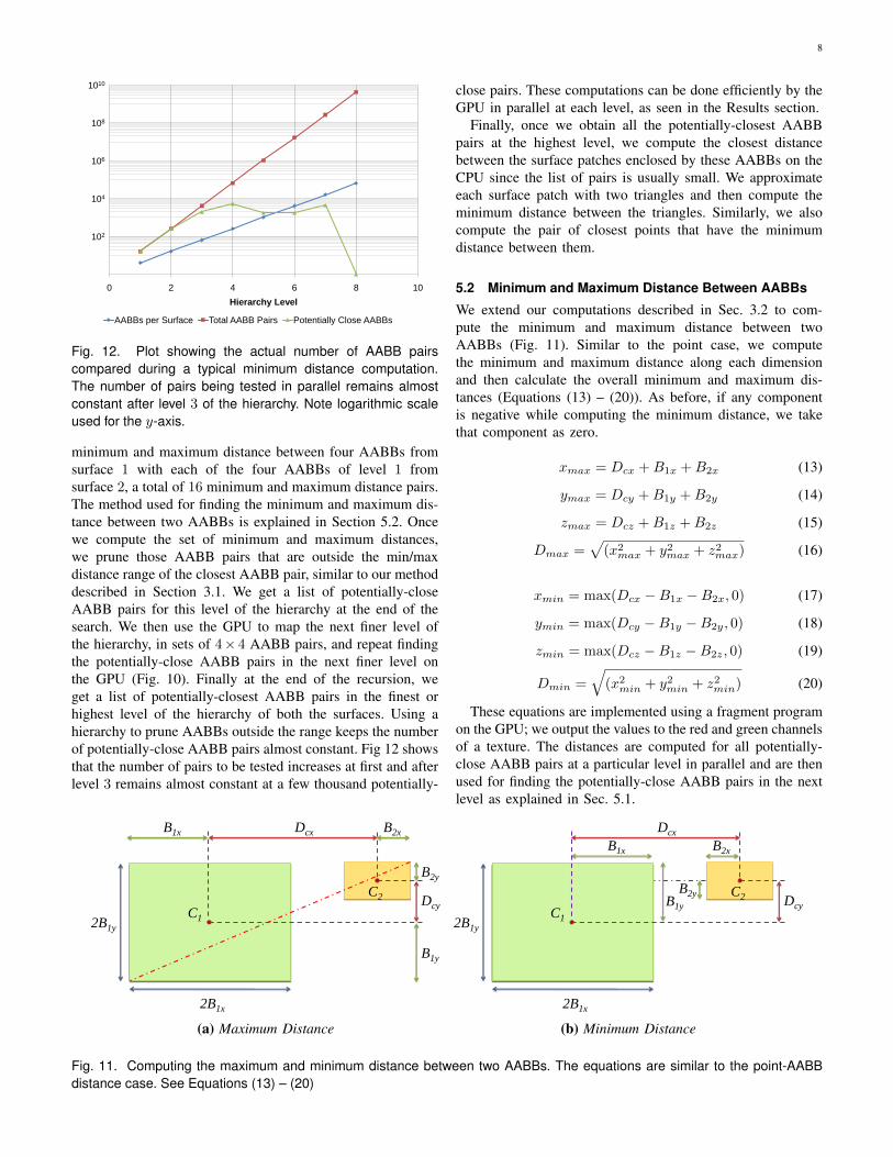
Fig. 12. Plot showing the actual number of AABB pairscompared during a typical minimum distance computation.The number of pairs being tested in parallel remains almostconstant after level 3 of the hierarchy. Note logarithmic scaleused for the y-axis.

minimum and maximum distance between four AABBs fromsurface 1 with each of the four AABBs of level 1 fromsurface 2, a total of 16 minimum and maximum distance pairs.The method used for finding the minimum and maximum dis-tance between two AABBs is explained in Section 5.2. Oncewe compute the set of minimum and maximum distances,we prune those AABB pairs that are outside the min/maxdistance range of the closest AABB pair, similar to our methoddescribed in Section 3.1. We get a list of potentially-closeAABB pairs for this level of the hierarchy at the end of thesearch. We then use the GPU to map the next finer level ofthe hierarchy, in sets of 4× 4 AABB pairs, and repeat findingthe potentially-close AABB pairs in the next finer level onthe GPU (Fig. 10). Finally at the end of the recursion, weget a list of potentially-closest AABB pairs in the finest orhighest level of the hierarchy of both the surfaces. Using ahierarchy to prune AABBs outside the range keeps the numberof potentially-close AABB pairs almost constant. Fig 12 showsthat the number of pairs to be tested increases at first and afterlevel 3 remains almost constant at a few thousand potentially-

close pairs. These computations can be done efficiently by theGPU in parallel at each level, as seen in the Results section.

Finally, once we obtain all the potentially-closest AABBpairs at the highest level, we compute the closest distancebetween the surface patches enclosed by these AABBs on theCPU since the list of pairs is usually small. We approximateeach surface patch with two triangles and then compute theminimum distance between the triangles. Similarly, we alsocompute the pair of closest points that have the minimumdistance between them.

5.2 Minimum and Maximum Distance Between AABBs

We extend our computations described in Sec. 3.2 to com-pute the minimum and maximum distance between twoAABBs (Fig. 11). Similar to the point case, we computethe minimum and maximum distance along each dimensionand then calculate the overall minimum and maximum dis-tances (Equations (13) – (20)). As before, if any componentis negative while computing the minimum distance, we takethat component as zero.

xmax = Dcx +B1x +B2x (13)

ymax = Dcy +B1y +B2y (14)

zmax = Dcz +B1z +B2z (15)

Dmax =√(x2max + y2max + z2max) (16)

xmin = max(Dcx −B1x −B2x, 0) (17)

ymin = max(Dcy −B1y −B2y, 0) (18)

zmin = max(Dcz −B1z −B2z, 0) (19)

Dmin =√(x2min + y2min + z2min) (20)

These equations are implemented using a fragment programon the GPU; we output the values to the red and green channelsof a texture. The distances are computed for all potentially-close AABB pairs at a particular level in parallel and are thenused for finding the potentially-close AABB pairs in the nextlevel as explained in Sec. 5.1.

Dcx

2B1x

B1y

2B1y

DcyC1

B1x B2x

C2

B2y

(a) Maximum Distance

Dcx

2B1x

B1y

2B1y

DcyC1

B1x B2x

C2B2y

(b) Minimum Distance

Fig. 11. Computing the maximum and minimum distance between two AABBs. The equations are similar to the point-AABBdistance case. See Equations (13) – (20)

9

5.3 Minimum Distance Between Two Trimmed NURBSSurfaces

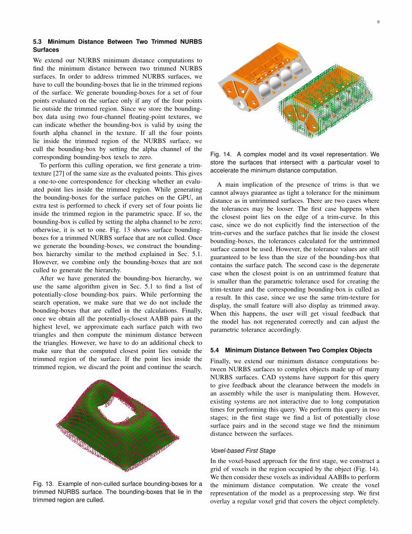
We extend our NURBS minimum distance computations tofind the minimum distance between two trimmed NURBSsurfaces. In order to address trimmed NURBS surfaces, wehave to cull the bounding-boxes that lie in the trimmed regionsof the surface. We generate bounding-boxes for a set of fourpoints evaluated on the surface only if any of the four pointslie outside the trimmed region. Since we store the bounding-box data using two four-channel floating-point textures, wecan indicate whether the bounding-box is valid by using thefourth alpha channel in the texture. If all the four pointslie inside the trimmed region of the NURBS surface, wecull the bounding-box by setting the alpha channel of thecorresponding bounding-box texels to zero.

To perform this culling operation, we first generate a trim-texture [27] of the same size as the evaluated points. This givesa one-to-one correspondence for checking whether an evalu-ated point lies inside the trimmed region. While generatingthe bounding-boxes for the surface patches on the GPU, anextra test is performed to check if every set of four points lieinside the trimmed region in the parametric space. If so, thebounding-box is culled by setting the alpha channel to be zero;otherwise, it is set to one. Fig. 13 shows surface bounding-boxes for a trimmed NURBS surface that are not culled. Oncewe generate the bounding-boxes, we construct the bounding-box hierarchy similar to the method explained in Sec. 5.1.However, we combine only the bounding-boxes that are notculled to generate the hierarchy.

After we have generated the bounding-box hierarchy, weuse the same algorithm given in Sec. 5.1 to find a list ofpotentially-close bounding-box pairs. While performing thesearch operation, we make sure that we do not include thebounding-boxes that are culled in the calculations. Finally,once we obtain all the potentially-closest AABB pairs at thehighest level, we approximate each surface patch with twotriangles and then compute the minimum distance betweenthe triangles. However, we have to do an additional check tomake sure that the computed closest point lies outside thetrimmed region of the surface. If the point lies inside thetrimmed region, we discard the point and continue the search.

Fig. 13. Example of non-culled surface bounding-boxes for atrimmed NURBS surface. The bounding-boxes that lie in thetrimmed region are culled.

Fig. 14. A complex model and its voxel representation. Westore the surfaces that intersect with a particular voxel toaccelerate the minimum distance computation.

A main implication of the presence of trims is that wecannot always guarantee as tight a tolerance for the minimumdistance as in untrimmed surfaces. There are two cases wherethe tolerances may be looser. The first case happens whenthe closest point lies on the edge of a trim-curve. In thiscase, since we do not explicitly find the intersection of thetrim-curves and the surface patches that lie inside the closestbounding-boxes, the tolerances calculated for the untrimmedsurface cannot be used. However, the tolerance values are stillguaranteed to be less than the size of the bounding-box thatcontains the surface patch. The second case is the degeneratecase when the closest point is on an untrimmed feature thatis smaller than the parametric tolerance used for creating thetrim-texture and the corresponding bounding-box is culled asa result. In this case, since we use the same trim-texture fordisplay, the small feature will also display as trimmed away.When this happens, the user will get visual feedback thatthe model has not regenerated correctly and can adjust theparametric tolerance accordingly.

5.4 Minimum Distance Between Two Complex Objects

Finally, we extend our minimum distance computations be-tween NURBS surfaces to complex objects made up of manyNURBS surfaces. CAD systems have support for this queryto give feedback about the clearance between the models inan assembly while the user is manipulating them. However,existing systems are not interactive due to long computationtimes for performing this query. We perform this query in twostages; in the first stage we find a list of potentially closesurface pairs and in the second stage we find the minimumdistance between the surfaces.

Voxel-based First Stage

In the voxel-based approach for the first stage, we construct agrid of voxels in the region occupied by the object (Fig. 14).We then consider these voxels as individual AABBs to performthe minimum distance computation. We create the voxelrepresentation of the model as a preprocessing step. We firstoverlay a regular voxel grid that covers the object completely.

10

Min/Max Distances

Map

List of Voxels

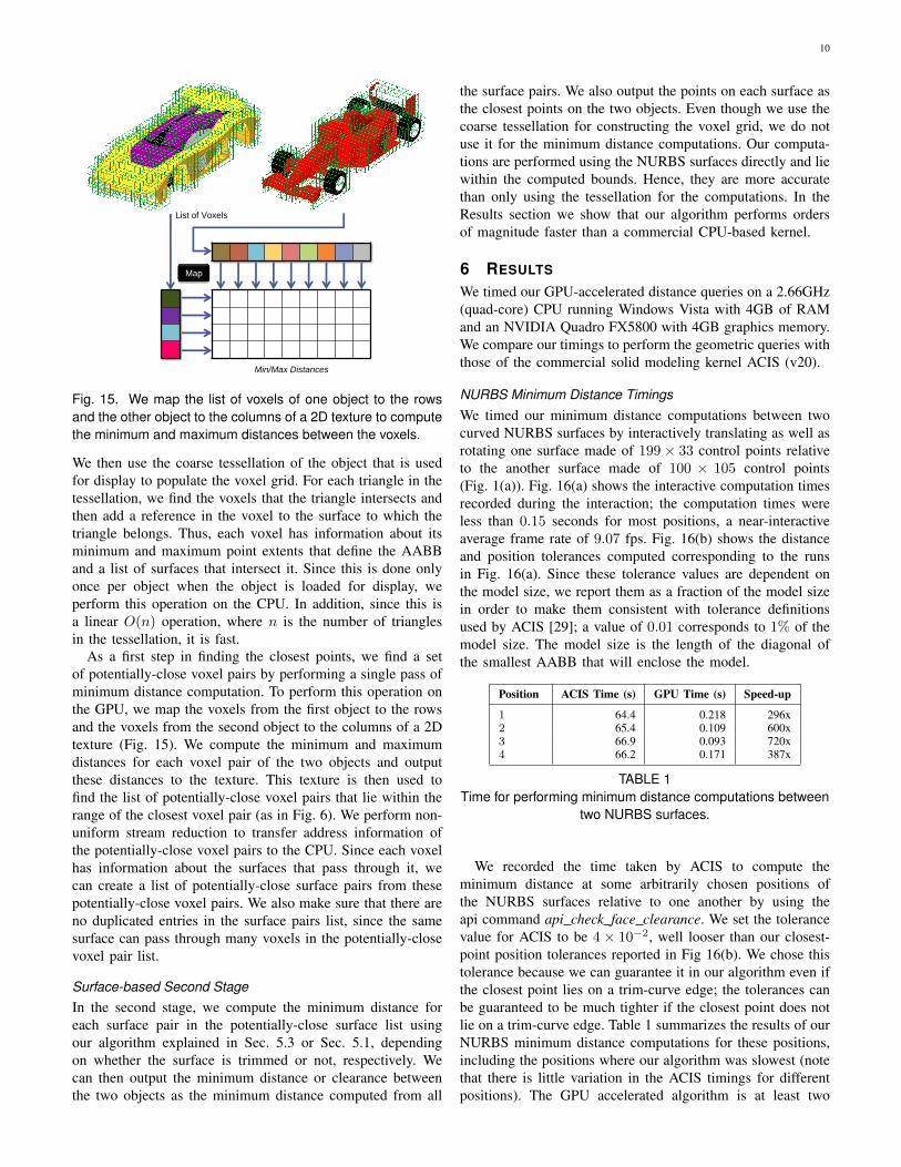
Fig. 15. We map the list of voxels of one object to the rowsand the other object to the columns of a 2D texture to computethe minimum and maximum distances between the voxels.

We then use the coarse tessellation of the object that is usedfor display to populate the voxel grid. For each triangle in thetessellation, we find the voxels that the triangle intersects andthen add a reference in the voxel to the surface to which thetriangle belongs. Thus, each voxel has information about itsminimum and maximum point extents that define the AABBand a list of surfaces that intersect it. Since this is done onlyonce per object when the object is loaded for display, weperform this operation on the CPU. In addition, since this isa linear O(n) operation, where n is the number of trianglesin the tessellation, it is fast.

As a first step in finding the closest points, we find a setof potentially-close voxel pairs by performing a single pass ofminimum distance computation. To perform this operation onthe GPU, we map the voxels from the first object to the rowsand the voxels from the second object to the columns of a 2Dtexture (Fig. 15). We compute the minimum and maximumdistances for each voxel pair of the two objects and outputthese distances to the texture. This texture is then used tofind the list of potentially-close voxel pairs that lie within therange of the closest voxel pair (as in Fig. 6). We perform non-uniform stream reduction to transfer address information ofthe potentially-close voxel pairs to the CPU. Since each voxelhas information about the surfaces that pass through it, wecan create a list of potentially-close surface pairs from thesepotentially-close voxel pairs. We also make sure that there areno duplicated entries in the surface pairs list, since the samesurface can pass through many voxels in the potentially-closevoxel pair list.

Surface-based Second StageIn the second stage, we compute the minimum distance foreach surface pair in the potentially-close surface list usingour algorithm explained in Sec. 5.3 or Sec. 5.1, dependingon whether the surface is trimmed or not, respectively. Wecan then output the minimum distance or clearance betweenthe two objects as the minimum distance computed from all

the surface pairs. We also output the points on each surface asthe closest points on the two objects. Even though we use thecoarse tessellation for constructing the voxel grid, we do notuse it for the minimum distance computations. Our computa-tions are performed using the NURBS surfaces directly and liewithin the computed bounds. Hence, they are more accuratethan only using the tessellation for the computations. In theResults section we show that our algorithm performs ordersof magnitude faster than a commercial CPU-based kernel.

6 RESULTS

We timed our GPU-accelerated distance queries on a 2.66GHz(quad-core) CPU running Windows Vista with 4GB of RAMand an NVIDIA Quadro FX5800 with 4GB graphics memory.We compare our timings to perform the geometric queries withthose of the commercial solid modeling kernel ACIS (v20).

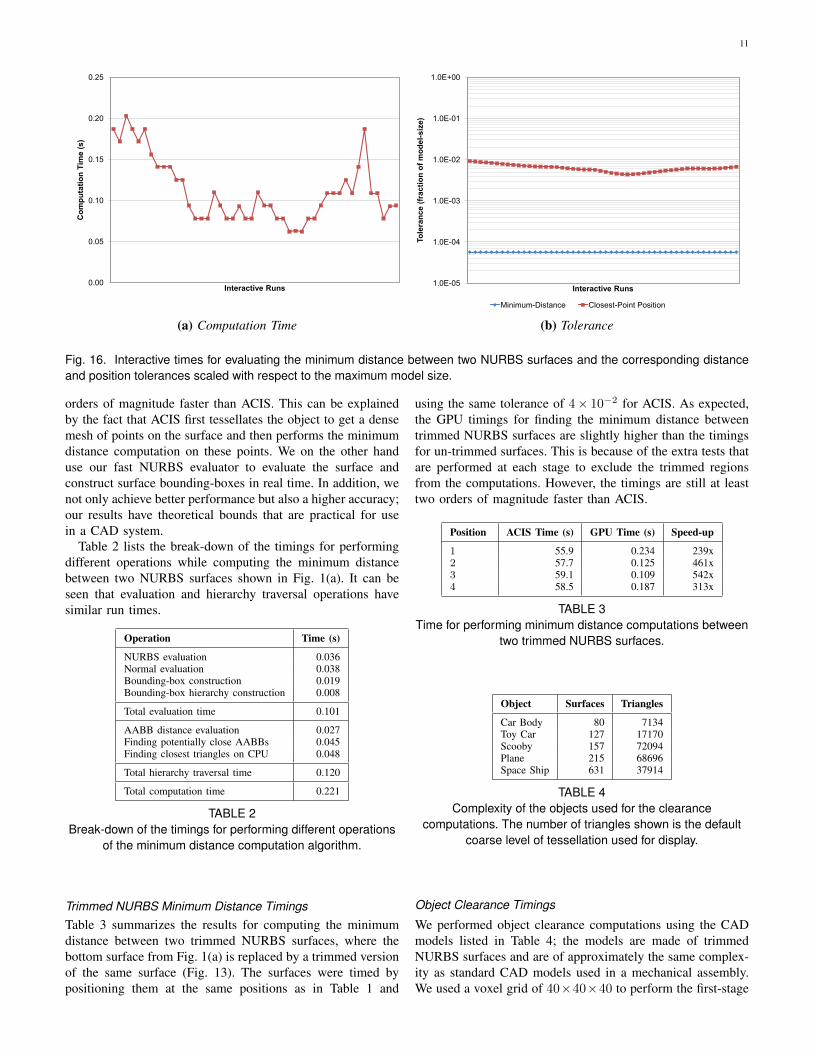
NURBS Minimum Distance TimingsWe timed our minimum distance computations between twocurved NURBS surfaces by interactively translating as well asrotating one surface made of 199× 33 control points relativeto the another surface made of 100 × 105 control points(Fig. 1(a)). Fig. 16(a) shows the interactive computation timesrecorded during the interaction; the computation times wereless than 0.15 seconds for most positions, a near-interactiveaverage frame rate of 9.07 fps. Fig. 16(b) shows the distanceand position tolerances computed corresponding to the runsin Fig. 16(a). Since these tolerance values are dependent onthe model size, we report them as a fraction of the model sizein order to make them consistent with tolerance definitionsused by ACIS [29]; a value of 0.01 corresponds to 1% of themodel size. The model size is the length of the diagonal ofthe smallest AABB that will enclose the model.

Position ACIS Time (s) GPU Time (s) Speed-up

1 64.4 0.218 296x2 65.4 0.109 600x3 66.9 0.093 720x4 66.2 0.171 387x

TABLE 1Time for performing minimum distance computations between

two NURBS surfaces.

We recorded the time taken by ACIS to compute theminimum distance at some arbitrarily chosen positions ofthe NURBS surfaces relative to one another by using theapi command api check face clearance. We set the tolerancevalue for ACIS to be 4× 10−2, well looser than our closest-point position tolerances reported in Fig 16(b). We chose thistolerance because we can guarantee it in our algorithm even ifthe closest point lies on a trim-curve edge; the tolerances canbe guaranteed to be much tighter if the closest point does notlie on a trim-curve edge. Table 1 summarizes the results of ourNURBS minimum distance computations for these positions,including the positions where our algorithm was slowest (notethat there is little variation in the ACIS timings for differentpositions). The GPU accelerated algorithm is at least two

11

0.00

0.05

0.10

0.15

0.20

0.25C

om

pu

tati

on

Tim

e (

s)

Interactive Runs

(a) Computation Time

1.0E-05

1.0E-04

1.0E-03

1.0E-02

1.0E-01

1.0E+00

To

lera

nc

e (

fra

cti

on

of

mo

de

l-s

ize

)

Interactive Runs

Minimum-Distance Closest-Point Position

(b) Tolerance

Fig. 16. Interactive times for evaluating the minimum distance between two NURBS surfaces and the corresponding distanceand position tolerances scaled with respect to the maximum model size.

orders of magnitude faster than ACIS. This can be explainedby the fact that ACIS first tessellates the object to get a densemesh of points on the surface and then performs the minimumdistance computation on these points. We on the other handuse our fast NURBS evaluator to evaluate the surface andconstruct surface bounding-boxes in real time. In addition, wenot only achieve better performance but also a higher accuracy;our results have theoretical bounds that are practical for usein a CAD system.

Table 2 lists the break-down of the timings for performingdifferent operations while computing the minimum distancebetween two NURBS surfaces shown in Fig. 1(a). It can beseen that evaluation and hierarchy traversal operations havesimilar run times.

Operation Time (s)

NURBS evaluation 0.036Normal evaluation 0.038Bounding-box construction 0.019Bounding-box hierarchy construction 0.008

Total evaluation time 0.101

AABB distance evaluation 0.027Finding potentially close AABBs 0.045Finding closest triangles on CPU 0.048

Total hierarchy traversal time 0.120

Total computation time 0.221

TABLE 2Break-down of the timings for performing different operations

of the minimum distance computation algorithm.

Trimmed NURBS Minimum Distance TimingsTable 3 summarizes the results for computing the minimumdistance between two trimmed NURBS surfaces, where thebottom surface from Fig. 1(a) is replaced by a trimmed versionof the same surface (Fig. 13). The surfaces were timed bypositioning them at the same positions as in Table 1 and

using the same tolerance of 4× 10−2 for ACIS. As expected,the GPU timings for finding the minimum distance betweentrimmed NURBS surfaces are slightly higher than the timingsfor un-trimmed surfaces. This is because of the extra tests thatare performed at each stage to exclude the trimmed regionsfrom the computations. However, the timings are still at leasttwo orders of magnitude faster than ACIS.

Position ACIS Time (s) GPU Time (s) Speed-up

1 55.9 0.234 239x2 57.7 0.125 461x3 59.1 0.109 542x4 58.5 0.187 313x

TABLE 3Time for performing minimum distance computations between

two trimmed NURBS surfaces.

Object Surfaces Triangles

Car Body 80 7134Toy Car 127 17170Scooby 157 72094Plane 215 68696Space Ship 631 37914

TABLE 4Complexity of the objects used for the clearance

computations. The number of triangles shown is the defaultcoarse level of tessellation used for display.

Object Clearance Timings

We performed object clearance computations using the CADmodels listed in Table 4; the models are made of trimmedNURBS surfaces and are of approximately the same complex-ity as standard CAD models used in a mechanical assembly.We used a voxel grid of 40×40×40 to perform the first-stage

12

Object1 Object2ACIS GPU Improvement

Time (s) Tolerance Time (s) Tolerance Time Tolerance

Toy Car Car Body 9.73 10−2 0.672 2.5× 10−5 14x 408xCar Body Car Body 17.34 10−2 0.439 2.2× 10−5 39x 463xScooby Scooby 70.62 10−1 0.382 13.7× 10−5 185x 728xPlane Plane 156.03 10−1 1.501 5.2× 10−5 104x 1938xPlane Space Ship 263.01 10−1 0.794 2.9× 10−5 331x 3453x

TABLE 5Time for performing minimum distance computations between different complex objects.

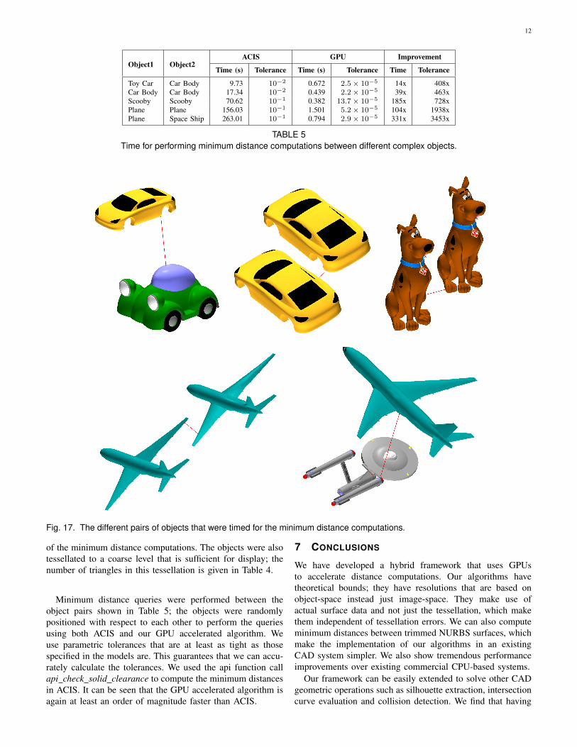
Fig. 17. The different pairs of objects that were timed for the minimum distance computations.

of the minimum distance computations. The objects were alsotessellated to a coarse level that is sufficient for display; thenumber of triangles in this tessellation is given in Table 4.

Minimum distance queries were performed between theobject pairs shown in Table 5; the objects were randomlypositioned with respect to each other to perform the queriesusing both ACIS and our GPU accelerated algorithm. Weuse parametric tolerances that are at least as tight as thosespecified in the models are. This guarantees that we can accu-rately calculate the tolerances. We used the api function callapi check solid clearance to compute the minimum distancesin ACIS. It can be seen that the GPU accelerated algorithm isagain at least an order of magnitude faster than ACIS.

7 CONCLUSIONS

We have developed a hybrid framework that uses GPUsto accelerate distance computations. Our algorithms havetheoretical bounds; they have resolutions that are based onobject-space instead just image-space. They make use ofactual surface data and not just the tessellation, which makethem independent of tessellation errors. We can also computeminimum distances between trimmed NURBS surfaces, whichmake the implementation of our algorithms in an existingCAD system simpler. We also show tremendous performanceimprovements over existing commercial CPU-based systems.

Our framework can be easily extended to solve other CADgeometric operations such as silhouette extraction, intersectioncurve evaluation and collision detection. We find that having

13

alternating serial and parallel stages and using the map-reducemotif for parallelism to be ideally suited for developing geo-metric algorithms that use the GPU. In addition, the parallelstages can be easily modified and executed on a multi-coreCPU in the absence of a powerful GPU. Our frameworkprovides for maximum flexibility and optimized performancein developing fast geometric algorithms.

ACKNOWLEDGMENTS

We would like to thank NVIDIA and AMD for providing uswith their hardware. The models used in the paper were down-loaded from 3D Content Central [30]. This material is basedupon work supported in part by SolidWorks Corporation, UCDiscovery under Grant No. DIG07-10224, and the NationalScience Foundation under CAREER Award No. 0547675.

APPENDIX

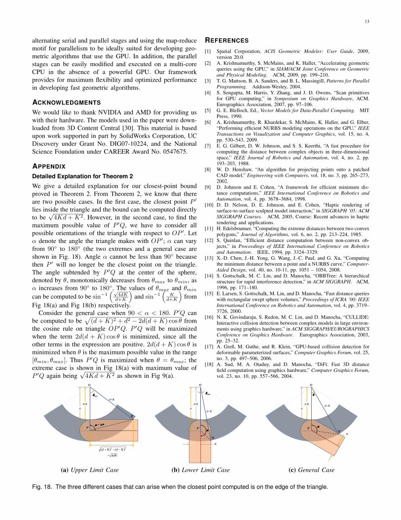
Detailed Explanation for Theorem 2

We give a detailed explanation for our closest-point boundproved in Theorem 2. From Theorem 2, we know that thereare two possible cases. In the first case, the closest point P ′

lies inside the triangle and the bound can be computed directlyto be

√4Kd+K2. However, in the second case, to find the

maximum possible value of P ′Q, we have to consider allpossible orientations of the triangle with respect to OP ′. Letα denote the angle the triangle makes with OP ′; α can varyfrom 90◦ to 180◦ (the two extremes and a general case areshown in Fig. 18). Angle α cannot be less than 90◦ becausethen P ′ will no longer be the closest point on the triangle.The angle subtended by P ′Q at the center of the sphere,denoted by θ, monotonically decreases from θmax to θmin, asα increases from 90◦ to 180◦. The values of θmax and θmin

can be computed to be sin−1(√

4dKd+K

)and sin−1

(K

d+K

)from

Fig 18(a) and Fig 18(b) respectively.Consider the general case when 90 < α < 180. P ′Q can

be computed to be√(d+K)2 + d2 − 2d(d+K) cos θ from

the cosine rule on triangle OP ′Q. P ′Q will be maximizedwhen the term 2d(d + K) cos θ is minimized, since all theother terms in the expression are positive. 2d(d+K) cos θ isminimized when θ is the maximum possible value in the range[θmin, θmax]. Thus P ′Q is maximized when θ = θmax; theextreme case is shown in Fig 18(a) with maximum value ofP ′Q again being

√4Kd+K2 as shown in Fig 9(a).

REFERENCES

[1] Spatial Corporation, ACIS Geometric Modeler: User Guide, 2009,version 20.0.

[2] A. Krishnamurthy, S. McMains, and K. Haller, “Accelerating geometricqueries using the GPU,” in SIAM/ACM Joint Conference on Geometricand Physical Modeling. ACM, 2009, pp. 199–210.

[3] T. G. Mattson, B. A. Sanders, and B. L. Massingill, Patterns for ParallelProgramming. Addison-Wesley, 2004.

[4] S. Sengupta, M. Harris, Y. Zhang, and J. D. Owens, “Scan primitivesfor GPU computing,” in Symposium on Graphics Hardware, ACM.Eurographics Association, 2007, pp. 97–106.

[5] G. E. Blelloch, Ed., Vector Models for Data-Parallel Computing. MITPress, 1990.

[6] A. Krishnamurthy, R. Khardekar, S. McMains, K. Haller, and G. Elber,“Performing efficient NURBS modeling operations on the GPU,” IEEETransactions on Visualization and Computer Graphics, vol. 15, no. 4,pp. 530–543, 2009.

[7] E. G. Gilbert, D. W. Johnson, and S. S. Keerthi, “A fast procedure forcomputing the distance between complex objects in three-dimensionalspace,” IEEE Journal of Robotics and Automation, vol. 4, no. 2, pp.193–203, 1988.

[8] W. D. Henshaw, “An algorithm for projecting points onto a patchedCAD model,” Engineering with Computers, vol. 18, no. 3, pp. 265–273,2002.

[9] D. Johnson and E. Cohen, “A framework for efficient minimum dis-tance computations,” IEEE International Conference on Robotics andAutomation, vol. 4, pp. 3678–3684, 1998.

[10] D. D. Nelson, D. E. Johnson, and E. Cohen, “Haptic rendering ofsurface-to-surface sculpted model interaction,” in SIGGRAPH ’05: ACMSIGGRAPH Courses. ACM, 2005, Course: Recent advances in hapticrendering and applications.

[11] H. Edelsbrunner, “Computing the extreme distances between two convexpolygons,” Journal of Algorithms, vol. 6, no. 2, pp. 213–224, 1985.

[12] S. Quinlan, “Efficient distance computation between non-convex ob-jects,” in Proceedings of IEEE International Conference on Roboticsand Automation. IEEE, 1994, pp. 3324–3329.

[13] X.-D. Chen, J.-H. Yong, G. Wang, J.-C. Paul, and G. Xu, “Computingthe minimum distance between a point and a NURBS curve,” Computer-Aided Design, vol. 40, no. 10-11, pp. 1051 – 1054, 2008.

[14] S. Gottschalk, M. C. Lin, and D. Manocha, “OBBTree: A hierarchicalstructure for rapid interference detection,” in ACM SIGGRAPH. ACM,1996, pp. 171–180.

[15] E. Larsen, S. Gottschalk, M. Lin, and D. Manocha, “Fast distance querieswith rectangular swept sphere volumes,” Proceedings of ICRA ’00: IEEEInternational Conference on Robotics and Automation, vol. 4, pp. 3719–3726, 2000.

[16] N. K. Govindaraju, S. Redon, M. C. Lin, and D. Manocha, “CULLIDE:Interactive collision detection between complex models in large environ-ments using graphics hardware,” in ACM SIGGRAPH/EUROGRAPHICSConference on Graphics Hardware. Eurographics Association, 2003,pp. 25–32.

[17] A. Greß, M. Guthe, and R. Klein, “GPU-based collision detection fordeformable parameterized surfaces,” Computer Graphics Forum, vol. 25,no. 3, pp. 497–506, 2006.

[18] A. Sud, M. A. Otaduy, and D. Manocha, “DiFi: Fast 3D distancefield computation using graphics hardware,” Computer Graphics Forum,vol. 23, no. 10, pp. 557–566, 2004.

max

Q

P´

O

d+K

= 90

2 2( ) ( )

= 4

d K d K

dK

d-K

d

(a) Upper Limit Case

Q

O

min

d+K

P´

d-K

d

K

(b) Lower Limit Case

Q

O

d+K

P´

d-K

d

K

(c) General Case

Fig. 18. The three different cases that can arise when the closest point computed is on the edge of the triangle.

14

[19] C. Lauterbach, M. Garland, S. Sengupta, D. Luebke, and D. Manocha,“Fast BVH construction on GPUs,” in Proceedings of Eurographics2009. Eurographics Association, 2009.

[20] P. Agarwal, S. Krishnan, N. Mustafa, and S. Venkatasubramanian,“Streaming geometric optimization using graphics hardware,” in 11thEuropean Symposium on Algorithms, 2003.

[21] K. E. Hoff, A. Zaferakis, M. Lin, and D. Manocha, “Fast and simple2D geometric proximity queries using graphics hardware,” in I3D ’01:Proceedings of the 2001 Symposium on Interactive 3D Graphics. ACM,2001, pp. 145–148.

[22] S. Briseid, T. Dokken, T. R. Hagen, and J. O. Nygaard, ComputationalScience - Lecture Notes in Computer Science. Springer, 2006, vol.3994/2006, ch. Spline Surface Intersections Optimized for GPUs, pp.204–211.

[23] T. Dokken, V. Skytt, T. R. Hagen, and J. O. Nygaard, US Patent20080259078 - Apparatus and Method for Determining Intersections,2005.

[24] S. Krishnan, M. Gopi, M. Lin, D. Manocha, and A. Pattekar, “Rapid and

accurate contact determination between spline models using shelltrees,”Computer Graphics Forum, vol. 17, no. 3, pp. 315–326, 1998.

[25] C. Lauterbach, Q. Mo, and D. Manocha, “gProximity: HierarchicalGPU-based operations for collision and distance queries,” in Proceedingsof Eurographics 2010, 2010, p. To Appear.

[26] A. Krishnamurthy, R. Khardekar, and S. McMains, “Direct evaluationof NURBS curves and surfaces on the GPU,” in ACM Symposium onSolid and Physical Modeling. ACM, 2007, pp. 329–334.

[27] ——, “Optimized GPU evaluation of arbitrary degree NURBS curvesand surfaces,” Computer Aided Design, vol. 41, no. 12, pp. 971–980,2009.

[28] D. Filip, R. Magedson, and R. Markot, “Surface algorithms using boundson derivatives,” Computer Aided Geometric Design, vol. 3, no. 4, pp.295–311, 1987.

[29] J. Corney and T. Lim, 3D Modeling with ACIS. Saxe-Coburg, 2001.[30] 3D Content Central, “http://www.3dcontentcentral.com,” 2009.