CONTRIBUTED RESEARCH ARTICLES 379

GMDH: An R Package for Short TermForecasting via GMDH-Type NeuralNetwork Algorithmsby Osman Dag and Ceylan Yozgatligil

Abstract Group Method of Data Handling (GMDH)-type neural network algorithms are the heuristicself organization method for the modelling of complex systems. GMDH algorithms are utilizedfor a variety of purposes, examples include identification of physical laws, the extrapolation ofphysical fields, pattern recognition, clustering, the approximation of multidimensional processes,forecasting without models, etc. In this study, the R package GMDH is presented to make short termforecasting through GMDH-type neural network algorithms. The GMDH package has options to usedifferent transfer functions (sigmoid, radial basis, polynomial, and tangent functions) simultaneouslyor separately. Data on cancer death rate of Pennsylvania from 1930 to 2000 are used to illustrate thefeatures of the GMDH package. The results based on ARIMA models and exponential smoothingmethods are included for comparison.

Introduction

Time series data are ordered successive observations which are measured in equally or unequallyspaced time. Time series data may include dependency among successive observations. Hence, theorder of the data is important. Time series data appear in various areas and disciplines such as medicalstudies, economics, the energy industry, agriculture, meteorology, and so on. Modelling time seriesdata utilizes the history of the data and makes forecasting using this history. At times, statisticalmodels are not sufficient to solve some problems. Examples include pattern recognition, forecasting,identification, etc. Extracting the information from the measurements has advantages while modellingcomplex systems when there is not enough prior information and/or no theory is defined to modelthe complex systems. Selecting a model automatically is a powerful way for the researchers who areinterested in the result and do not have sufficient statistical knowledge and sufficient time (Muelleret al., 1998) for an analysis.

The objective of this study is to develop an R package for forecasting of time series data. Some ofrecent softwares developed for time series are glarma, ftsa, MARSS, ensembleBMA, ProbForecast-GOP, and forecast (Dunsmuir and Scott, 2015; Shang, 2013; Holmes et al., 2012; Fraley et al., 2011;Hyndman and Khandakar, 2008). In this study, we focused on the development of an R packagefor short term forecasting via Group Method of Data Handling (GMDH) algorithms. The history ofGMDH-type neural network is based on works from the end of the 1960s and the beginning of the1970s. First, Ivakhnenko (1966) introduced a polynomial, which is the basic algorithm of GMDH, toconstruct higher order polynomials. Also, Ivakhnenko (1970) introduced heuristic self-organizationmethods which constructed the main working system of GMDH algorithm. Heuristic self-organizationmethod defines the way that the algorithm evolves, following rules such as external criteria. TheGMDH method, convenient for complex and unstructured systems, has benefits over high orderregression (Farlow, 1981).

Kondo (1998) proposed GMDH-type neural network in which the algorithm works accordingto the heuristic self-organization method. Kondo and Ueno (2006a,b) proposed a GMDH algorithmwhich has a feedback loop. According to this algorithm, the output obtained from the last layer is setas a new input variable, provided a threshold is not satisfied in the previous layer. The system of thealgorithm is organized by a heuristic self-organization method where a sigmoid transfer function isintegrated. Kondo and Ueno (2007) proposed a logistic GMDH-type neural network. The differencefrom a conventional GMDH algorithm was that the new one would take linear functions of all inputsat the last layer. Kondo and Ueno (2012) included three transfer functions (sigmoid, radial basis andpolynomial functions) in the feedback GMDH algorithm. Srinivasan (2008) used a GMDH-type neuralnetwork and traditional time series models to forecast predicted energy demand. It was shown thata GMDH-type neural network was superior in forecasting energy demand compared to traditionaltime series models with respect to mean absolute percentage error (MAPE). In another study, Xu et al.(2012) applied a GMDH algorithm and ARIMA models to forecast the daily power load. According totheir results, GMDH-based results were superior to the results of ARIMA models in terms of MAPEfor forecasting performance.

There are some difficulties when applying a GMDH-type neural network. For example, there is nofreely available software for researchers implementing the GMDH algorithms in the literature. We

The R Journal Vol. 8/1, Aug. 2016 ISSN 2073-4859

CONTRIBUTED RESEARCH ARTICLES 380

present the R package GMDH to make short term forecasting through GMDH-type neural networkalgorithms. The package includes two types of GMDH structures; namely, GMDH structure andrevised GMDH (RGMDH) structure. Also, it includes a variety of options to use different transferfunctions (sigmoid, radial basis, polynomial, and tangent functions) simultaneously or separately. Dataon the cancer death rate of Pennsylvania from 1930 to 2000 are used to illustrate the implementation ofGMDH package. We compare the results to those based on ARIMA models and exponential smoothing(ES) methods.

Methodology

In this section, data preparation, two types of GMDH-type neural network structures, and estimationof a regularization parameter in regularized least square estimation (RLSE) are given.

Data preparation

Data preparation has an important role in GMDH-type neural network algorithms. To get rid of verybig numbers in calculations and to be able to use all transfer functions in the algorithm, it is necessaryfor range of the data to be in the interval of (0, 1). If αt is the actual time series dataset at hand, thisnecessity is guaranteed by the following transformation,

wt =αt + δ1

δ2(1)

with

δ1 =

{|αt|+ 1 if min(αt) ≤ 0

0 if min(αt) > 0

and

δ2 = max(αt + δ1) + 1.

During the estimation and forecasting process in GMDH-type neural network algorithms, all calcu-lations are done using the scaled data set, wt. After all processes are ended–i.e, all predictions andforecasts are obtained–we apply the inverse transformation as follows,

αt = wt × δ2 − δ1. (2)

Let’s assume a time series dataset for t time points, and p inputs. An illustration of time seriesdata structure in GMDH algorithms is presented in Table 1. Since we construct the model for the datawith time lags, the number of observations, presented under the subject column in the table, is equalto t− p; and the number of inputs, lagged time series, is p. In this table, the variable called z is put inthe models as a response variable, and the rest of the variables are taken into models as lagged timeseries xi, where i = 1, 2, ..., p. The notations in Table 1 are followed throughout this paper.

Table 1: An illustration of time series data structure in GMDH algorithms

Subject z x1 x2 . . . xp1 wt wt−1 wt−2 . . . wt−p2 wt−1 wt−2 wt−3 . . . wt−p−13 wt−2 wt−3 wt−4 . . . wt−p−2...

......

.... . .

...t− p wp+1 wp wp−1 . . . w1

A better model which explains the relation between response and lagged time series is capturedvia transfer functions. The sigmoid, radial basis, polynomial, and tangent functions, presented in Table2, are mainly used to explain the relation between inputs and output in GMDH-type neural networkalgorithms (Kondo and Ueno, 2012). We use all transfer functions, stated in Table 2, simultaneously ineach neuron. In other words, we construct four models at each neuron, and then the model whichgives the smallest prediction mean square error (PMSE) is selected as the current transfer function atthe corresponding neuron.

The R Journal Vol. 8/1, Aug. 2016 ISSN 2073-4859

CONTRIBUTED RESEARCH ARTICLES 381

Table 2: Transfer functions

Sigmoid Function z = 1/(1 + e−y)

Radial Basis Function z = e−y2

Polynomial Function z = yTangent Function z = tan(y)

GMDH algorithm

GMDH-type neural network algorithms are modeling techniques which learn the relations among thevariables. In the perspective of time series, the algorithm learns the relationship among the lags. Afterlearning the relations, it automatically selects the way to follow in algorithm. First, GMDH was usedby Ivakhnenko (1966) to construct a high order polynomial. The following equation is known as theIvakhnenko polynomial given by

y = a +m

∑i=1

bi · xi +m

∑i=1

m

∑j=1

cij · xi · xj +m

∑i=1

m

∑j=1

m

∑k=1

dijk · xi · xj · xk + . . . (3)

where m is the number of variables and a, b, c, d, . . . are coeffients of variables in the polynomial, alsonamed as weights. Here, y is a response variable, xi and xj are the lagged time series to be regressed.In general, the terms are used in calculation up to square terms as presented below,

y = a +m

∑i=1

bi · xi +m

∑i=1

m

∑j=1

cij · xi · xj (4)

The GMDH algorithm considers all pairwise combinations of p lagged time series. Therefore,each combination enters each neuron. Using these two inputs, a model is constructed to estimate thedesired output. In other words, two input variables go in a neuron, one result goes out as an output.The structure of the model is specified by Ivakhnenko polynomial in equation 4 where m = 2. Thisspecification requires that six coefficients in each model are to be estimated.

The GMDH algorithm is a system of layers in which there exist neurons. The number of neuronsin a layer is defined by the number of input variables. To illustrate, assume that the number of inputvariables is equal to p, since we include all pairwise combinations of input variables, the number ofneurons is equal to h = (p

2). The architecture of GMDH algorithm is illustrated in Figure 1 when thereare three layers and four inputs.

Figure 1: Architecture of GMDH algorithm

In the GMDH architecture shown in Figure 1, since the number of inputs is equal to four, thenumber of nodes in a layer is determined to be six. This is just a starting layer to the algorithm. Thecoefficients of equation 4 are estimated in each neuron. By using the estimated coefficients and inputvariables in each neuron, the desired output is predicted. According to a chosen external criteria, p

The R Journal Vol. 8/1, Aug. 2016 ISSN 2073-4859

CONTRIBUTED RESEARCH ARTICLES 382

neurons are selected and h− p neurons are eliminated from the network. In this study, predictionmean square error (PMSE) is used as the external criteria. In Figure 1, four neurons are selected whiletwo neurons are eliminated from the network. The outputs obtained from selected neurons becomethe inputs for the next layer. This process continues until the last layer. At the last layer, only oneneuron is selected. The obtained output from the last layer is the predicted value for the time series athand. The flowchart of the algorithm is depicted in Figure 2.

Figure 2: Flowchart of GMDH algorithms

In a GMDH algorithm, there exist six coefficients to be estimated in each model. Coefficients areestimated via RLSE.

RGMDH algorithm

A GMDH-type neural network constructs the algorithm by investigating the relation between twoinputs and the desired output. Architecture of a revised GMDH (RGMDH)-type neural network doesnot only consider this relation, but it also considers the individual effects on the desired output (Kondoand Ueno, 2006b). There are two different types of neurons in an RGMDH-type neural network. In thefirst type of neuron, it is same as in GMDH-type neural network, given as in equation 4. That is, twoinputs enter the neuron, one output goes out. In the second type of neuron, r inputs enter the neuron,one output goes out. This second type neuron is given by

y = a +r

∑i=1

bi · xi , r ≤ p, (5)

where r is the number of inputs in the corresponding second type neuron.

As mentioned above, there exist h = (p2) neurons in one layer in a GMDH-type neural network.

In addition to this, with the p neurons from the second type of neuron, the number of neurons inone layer becomes η = (p

2) + p in an RGMDH-type algorithm. The architecture of an RGMDH-typealgorithm is shown in Figure 3 for the case when there are three layers and three inputs. In thisarchitecture, since the number of inputs is three, the number of nodes in a layer is determined to be six.Here, three of six nodes are the first type of neurons in which all pairwise combinations of lagged timeseries are already used as in the GMDH algorithm. The rest of the three nodes are the second typeof neurons where the individual effects of the lagged time series are sequentially added to the layerstarting from lag 1. In each neuron, coefficients of models are calculated by using the correspondingmodels in equations 4 and 5. For instance, in Figure 3, there are six coefficients to be estimated as givenby equation 4 for the first type of neurons, and two, three and four coefficients are estimated as givenin equation 5 for the the second type of neurons when r equals to 1, 2 and 3, respectively. The desiredoutput is predicted by utilizing estimated coefficients and input variables in each neuron. Here, pneurons are selected as living cells and η − p death cells are eliminated from the network according tothe external criteria. The rest of the algorithm is same with GMDH.

The R Journal Vol. 8/1, Aug. 2016 ISSN 2073-4859

CONTRIBUTED RESEARCH ARTICLES 383

Figure 3: Architecture of an RGMDH algorithm

Estimation of regularization parameter in RLSE

In each estimation step, there exist the coefficients to be estimated. While we are estimating thesecoefficients, we use the regularized least square estimation method. It is stated that regularized leastsquare estimation is utilized when there is the possibility of a multi-collinearity problem by integratinga regularization parameter, λ, into the estimation step. It is important to note that regularized leastsquare estimation differs from the least square estimation when the regularization parameter is notzero.

We integrate the estimation of a regularization parameter (penalizing term) via validation inGMDH algorithms. For this purpose, we divide the data into two parts: a learning set and a testing set.In the GMDH package, 70% of the time series, by default, is taken for the learning set. Since the dataset is time dependent, the order of data is saved in this division process. In other words, by default,the first 70% of the data is used for learning set and the last 30% of the data is utilized as a testingset. This whole process is applied for each model constructed in each neuron. The algorithm for theregularization parameter estimation is as follows:

i) Clarify the possible regularization parameter, λ = 0, 0.01, 0.02, 0.04, 0.08, . . . , 10.24. Note that,when λ = 0, RLSE is converted to LSE.

ii) For each possible λ value, coefficients are estimated via RLSE by using the learning set.

iii) After the calculation of coefficients, calculate the predicted values by utilizing the test set to obtainthe MSE for each regularization parameter.

iv) Select the regularization parameter which gives the minimum MSE value.

Implementation of GMDH package

The data used in this application of the GMDH package are the yearly cancer death rate (per 100,000population) in the Pennsylvania between 1930 and 2000. The data were documented in PennsylvaniaVital Statistics Annual Report by the Pennsylvania Department of Health in 2000 (Wei, 2006). Thisdataset is also available as a dataset in the package GMDH. After installing the GMDH package, itcan be loaded into an R workspace by

R> library("GMDH")R> data("cancer") # load cancer data

After the cancer death rate data set is loaded, one may use fcast function in GMDH package forshort-term forecasting. To utilize the GMDH structure for forecasting, method is set to "GMDH". Oneshould set the method to "RGMDH" to use the RGMDH structure.

The R Journal Vol. 8/1, Aug. 2016 ISSN 2073-4859

CONTRIBUTED RESEARCH ARTICLES 384

R> out = fcast(cancer[1:66], method = "GMDH", input = 15, layer = 1, f.number = 5,level = 95, tf = "all", weight = 0.70, lambda = c(0, 0.01, 0.02, 0.04, 0.08, 0.16,0.32, 0.64, 1.28, 2.56, 5.12, 10.24))

Point Forecast Lo 95 Hi 9567 249.5317 244.9798 254.083668 249.6316 244.4891 254.774169 248.9278 243.0318 254.823970 247.0385 240.7038 253.373171 244.7211 237.1255 252.3168

# display fitted valuesR> out$fitted

# return residualsR> out$residuals

# show forecastsR> out$mean

In this part, we divided the data into two parts for the aim of observing the ability of methodson prediction (n = 66) and forecasting (n = 5). We include ARIMA models and ES methods forcomparison purpose. For the determination of the best order of ARIMA models and the best methodof ES techniques, there are two functions in the R package forecast. These functions, auto.arima andets, which use grid search, select the best model according to the criteria of either AIC, AICc or BIC.For this data set, the functions suggested the model ARIMA (1, 1, 0) with intercept and an ES methodwith multiplicative errors, additive damped trend and no seasonality (M, Ad, N), respectively. Wealso added the model ARIMA (0, 1, 0) with intercept for this data set suggested by Wei (2006). For allmodels, prediction mean square error (PMSE) and forecasting mean square error (FMSE) are stated inTable 3.

Figure 4: Yearly cancer death rate (per 100,000 population) in Pennsylvania between 1941 and 2000with predictions and forecasts obtained via RGMDH and ES(M,Ad,N)

The R Journal Vol. 8/1, Aug. 2016 ISSN 2073-4859

CONTRIBUTED RESEARCH ARTICLES 385

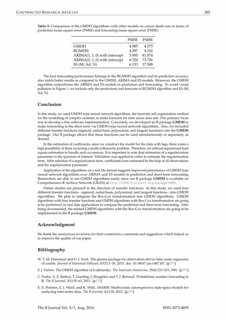
Table 3: Comparison of the GMDH algorithms with other models on cancer death rate in terms ofprediction mean square error (PMSE) and forecasting mean square error (FMSE)

PMSE FMSE

GMDH 4.985 4.575RGMDH 4.287 4.102ARIMA(1, 1, 0) with intercept 5.995 81.874ARIMA(0, 1, 0) with intercept 6.324 73.756ES (M, Ad, N) 6.153 17.508

The best forecasting performance belongs to the RGMDH algorithm and its prediction accuracyalso yields better results as compared to the GMDH, ARIMA and ES models. Moreover, the GMDHalgorithm outperforms the ARIMA and ES models in prediction and forecasting. To avoid visualpollution in Figure 4, we include only the predictions and forecasts of RGMDH algorithm and ES (M,Ad, N).

Conclusion

In this study, we used GMDH-type neural network algorithms, the heuristic self-organization methodfor the modelling of complex systems, to make forecasts for time series data sets. Our primary focuswas to develop a free software implementation. Concretely, we developed an R package GMDH tomake forecasting in the short term via GMDH-type neural network algorithms. Also, we includeddifferent transfer functions (sigmoid, radial basis, polynomial, and tangent functions) into the GMDHpackage. Our R package allows that these functions can be used simultaneously or separately, asdesired.

In the estimation of coefficients, since we construct the model for the data with lags, there exists ahigh possibility of there occurring a multi-collinearity problem. Therefore, we utilized regularized leastsquare estimation to handle such occurences. It is important to note that estimation of a regularizationparameter is the question of interest. Validation was applied in order to estimate the regularizationterm. After selection of a regularization term, coefficients were estimated by the help of all observationsand the regularization parameter.

Application of the algorithms on a real life dataset suggests improved performance of GMDH-typeneural network algorithms over ARIMA and ES models in prediction and short term forecasting.Researchers are able to use GMDH algorithms easily since our R package GMDH is available onComprehensive R Archive Network (CRAN) at http://CRAN.R-project.org/package=GMDH.

Future studies are planned in the direction of transfer functions. In this study, we used fourdifferent transfer functions - sigmoid, radial basis, polynomial, and tangent functions - into GMDHalgorithms. We plan to integrate the Box-Cox transformation into GMDH algorithms. GMDHalgorithms with four transfer functions and GMDH algorithms with Box-Cox transformation are goingto be performed on real data applications to compare the prediction and short term forecasting. Afterbeing documented, the related GMDH algorithms with the Box-Cox transformation are going to beimplemented in the R package GMDH.

Acknowledgment

We thank the anonymous reviewers for their constructive comments and suggestions which helped usto improve the quality of our paper.

Bibliography

W. T. M. Dunsmuir and D. J. Scott. The glarma package for observation-driven time series regressionof counts. Journal of Statistical Software, 67(7):1–36, 2015. doi: 10.18637/jss.v067.i07. [p379]

S. J. Farlow. The GMDH algorithm of Ivakhnenko. The American Statistician, 35(4):210–215, 1981. [p379]

C. Fraley, A. E. Raftery, T. Gneiting, J. Sloughter, and V. J. Berrocal. Probabilistic weather forecasting inR. The R Journal, 3(1):55–63, 2011. [p379]

E. E. Holmes, E. J. Ward, and K. Wills. MARSS: Multivariate autoregressive state-space models foranalyzing time-series data. The R Journal, 4(1):30, 2012. [p379]

The R Journal Vol. 8/1, Aug. 2016 ISSN 2073-4859

CONTRIBUTED RESEARCH ARTICLES 386

R. Hyndman and Y. Khandakar. Automatic time series forecasting: The forecast package for R. Journalof Statistical Software, 27(3):1–22, 2008. [p379]

A. Ivakhnenko. The group method of data handling–a rival of the method of stochastic approximation.Soviet Automatic Control, 13(3):43–55, 1966. [p379, 381]

A. Ivakhnenko. Heuristic self-organization in problems of engineering cybernetics. Automatica, 6(2):207–219, 1970. [p379]

T. Kondo. GMDH neural network algorithm using the heuristic self-organization method and itsapplication to the pattern identification problem. In SICE’98. Proceedings of the 37th SICE AnnualConference. International Session Papers, pages 1143–1148. IEEE, 1998. [p379]

T. Kondo and J. Ueno. Medical image recognition of the brain by revised GMDH-type neural networkalgorithm with a feedback loop. International Journal of Innovative Computing, Information and Control,2(5):1039–1052, 2006a. [p379]

T. Kondo and J. Ueno. Revised gmdh-type neural network algorithm with a feedback loop identifyingsigmoid function neural network. International Journal of Innovative Computing, Information andControl, 2(5):985–996, 2006b. [p379, 382]

T. Kondo and J. Ueno. Logistic GMDH-type neural network and its application to identification ofX-ray film characteristic curve. JACIII, 11(3):312–318, 2007. [p379]

T. Kondo and J. Ueno. Feedback GMDH-type neural network and its application to medical imageanalysis of liver cancer. In 42th ISCIE international symposium on stochastic systems theory and itsapplications, pages 81–82, 2012. [p379, 380]

J. A. Mueller, A. Ivachnenko, and F. Lemke. GMDH algorithms for complex systems modelling.Mathematical and Computer Modelling of Dynamical Systems, 4(4):275–316, 1998. [p379]

H. L. Shang. ftsa: An R package for analyzing functional time series. The R Journal, 5(1):64–72, 2013.URL http://journal.r-project.org/archive/2013-1/shang.pdf. [p379]

D. Srinivasan. Energy demand prediction using GMDH networks. Neurocomputing, 72(1):625–629,2008. [p379]

W. W. S. Wei. Time series analysis: univariate and multivariate methods. Addison-Wesley publ, 2006. [p383,384]

H. Xu, Y. Dong, J. Wu, and W. Zhao. Application of GMDH to short-term load forecasting. In Advancesin Intelligent Systems, pages 27–32. Springer-Verlag, 2012. [p379]

Osman DagDepartment of BiostatisticsFaculty of MedicineHacettepe University06100 Ankara, Turkeyosman.dag@hacettepe.edu.tr

Ceylan YozgatligilDepartment of StatisticsFaculty of Arts and SciencesMiddle East Technical University06531 Ankara, Turkeyceylan@metu.edu.tr

The R Journal Vol. 8/1, Aug. 2016 ISSN 2073-4859