global optimization with unknown lipschitz constant · dann ist unklar, welche methode benutzt...
TRANSCRIPT

Global optimization withunknown Lipschitz constant
Dissertation
zur Erlangung des akademischen Grades
doctor rerum naturalium (Dr. rer. nat.)
vorgelegt dem Rat
der Fakultat fur Mathematik und Informatik
der Friedrich-Schiller-Universitat Jena
von Dipl.-Math. Matthias Ulrich Horn
geboren am 11. Mai 1975 in Frankfurt am Main

Gutachter
1. Prof. Dr. Erich Novak
2. Prof. Dr. James M. Calvin
Tag der letzten Prufung des Rigorosums: 07. Oktober 2005
Tag der offentlichen Verteidigung: 13. Oktober 2005

Zusammenfassung
Wir betrachten das globale Optimierungsproblem, d.h. fur eine reellwertigeund beschrankte Funktion f suchen wir eine Stelle x des Definitionsbereichs,deren Funktionswert f(x) nahe dem Infimum inf f liegt. Wir untersuchenden Fall, daß f eine d-variate, Lipschitz-stetige Funktion ist, die in einemgewissen Sinne in der Nahe der globalen Minimalstelle(n) nicht zu langsamwachst. Wir leisten zwei Beitrage:
• Wir zeigen, daß fur eine optimale Methode Adaptivitat notwendig istund daß Randomisierung (Monte Carlo) keine weiteren Vorteile bringt.
• Wir stellen eine Methode vor, die universell ist im folgenden Sinne:Diese Methode hat die optimale Konvergenzrate auch in dem Fall,daß weder die Lipschitzkonstante noch die ubrigen Klassenparameterbekannt sind.
Im folgenden werden wir detaillierter. Wir betrachten Funktionen
f : [0, 1]d → R,
die die folgenden zwei Eigenschaften haben:
1. Die Funktion f ist Lipschitz-stetig mit Lipschitzkonstante L > 0:
∀x, y ∈ [0, 1]d |f(x) − f(y)| ≤ L‖x− y‖∞.
Hier bezeichnet ‖ · ‖∞ die Maximumsnorm.
2. Sei λd das Lebesgue-Maß auf [0, 1]d. Fur die Niveaumengen
A(f, δ) := x ∈ [0, 1]d : f(x) ≤ inf f + δ
existieren Konstanten %,D > 0, sodaß
∀ 0 ≤ δ ≤ % λd(A(f, δ)) ≤ D δd/2.
iii

iv ZUSAMMENFASSUNG
Wir sagen f ∈ F dL,D,%. Wir erwahnen einige Merkmale dieser Problem-
klasse: Eine Funktion f ∈ F dL,D,% kann mehrere Minimalstellen haben. Als
Glattheit wird nur Lipschitz-Stetigkeit gefordert. Weiterhin kann man zujeder zweifach stetig differenzierbaren Funktion, die an jeder von endlich vie-len Minimalstellen eine positiv definite Hesse-Matrix hat, Parameter L,D, %finden, sodaß f ∈ F d
L,D,%. Wir diskutieren die Problemklasse F dL,D,% ausfuhrlich
in Chapter 1.
Fur F dL,D,% schlagen wir zwei adaptive Optimierungsalgorithmen vor, die
wir in Chapter 2 vorstellen. Der erste findet Anwendung in der Situation,daß die Lipschitzkonstante oder eine obere Schranke fur sie bekannt ist. Diebeiden anderen Klassenparameter D und % fließen nicht in die Definition desAlgorithmus ein und brauchen nicht bekannt sein. Sie sind allerdings wichtigfur eine Abschatzung der Kosten.
Zusatzlich kann es vorkommen, daß auch fur die Lipschitzkonstante keineInformation vorliegt. Dann ist unklar, welche Methode benutzt werden soll.Von einem praktischen Standpunkt aus gesehen sind deshalb solche Algo-rithmen von Interesse, die fur viele Problemklassen gute Ergebnisse liefern.Der zweite von uns vorgeschlagene Algorithmus kann auch dann angewendetwerden, falls wir keine Information uber L haben. Tatsachlich konvergiert erfur alle stetigen Funktionen.
In Chapter 3 vergleichen wir unsere Algorithmen mit moglicherweisebesseren Algorithmen. Die Methoden, die wir dabei betrachten, haben zweiwesentliche Merkmale:
1. Ein Algorithmus kann reelle Zahlen exakt verarbeiten und speichern.
2. Ein Algorithmus kann eine endliche Anzahl Funktionswerte benutzen,d.h. er hat nur partielle Information uber die Zielfunktion.
Wir unterscheiden zwischen adaptiven und nichtadaptiven Methoden, je nach-dem, wie der Algorithmus die Auswertungsstellen bestimmt.
Eine grundlegende Frage in der Numerik ist, ob adaptive Methoden we-sentlich besser sind als nichtadaptive. Um diese Frage zu beantworten, fuhrenwir zunachst die Begriffe Kosten und Fehler ein. Fur einen Algorithmus Adefinieren wir cost(A, F d
L,D,%) als die im worst case benotigte Anzahl Funk-tionswerte, um fur f ∈ F d
L,D,% eine Naherungslosung zu liefern. Gibt Afur f die Naherungslosung x zuruck, so ist der funktionsweise Fehler mit∆(A, f) := f(x) − inf f gegeben. Der Fehler ∆(A, F d
L,D,%) ist der worst caseFehler fur f ∈ F d
L,D,%. Die Fehlerzahlen
eadn (F dL,D,%) := inf ∆(A, F d
L,D,%) : A ad. Meth., cost(A, F dL,D,%) ≤ n,
ZUSAMMENFASSUNG v
enonn (F d
L,D,%) := inf ∆(A, F dL,D,%) : A nichtad. Meth., cost(A, F d
L,D,%) ≤ nsind die Werkzeuge, um die obige Frage zu beantworten. Wir sagen, adaptiveMethoden sind wesentlich besser als nichtadaptive, falls
limn→∞
eadn (F dL,D,%)
enonn (F d
L,D,%)= 0.
Wir zitieren einige bekannte Komplexitatsergebnisse in Section 3.2, insbeson-dere fur Klassen, die Ahnlichkeiten zu unserer haben. Fur F d
L,D,% zeigen wir
eadn (F dL,D,%) n−2/d,
enonn (F d
L,D,%) n−1/d.
Insbesondere liefern also adaptive Methoden einen quadratischen speed-upgegenuber nichtadaptiven.
Eine weitere grundlegende Frage in der Numerik ist, ob Randomisierung(Monte Carlo) eine zusatzliche Verbesserung der Konvergenzrate ermoglicht.Wir betrachten randomisierte Methoden und weisen nach, daß sie die Konver-genzgeschwindigkeit nicht wesentlich erhohen konnen.
Ein Hauptbeitrag dieser Arbeit beschaftigt sich mit Universalitat. Wirsagen, eine Methode A ist universell fur eine Familie F von Problemklassen,falls A fur jede Klasse aus F die optimale Konvergenzrate hat. Wir zeigen,daß unser zweiter Algorithmus universell ist fur (F d
L,D,%). Weiterhin zeigenwir, daß unser erster Algorithmus die optimale Konvergenzrate hat, falls dieLipschitzkonstante bekannt ist.
Es scheint, daß das Thema Universalitat in der globalen Optimierungzuvor nicht betrachtet wurde. Die Artikel, die wir finden konnten und diesich mit universellen Methoden beschaftigen, betrachten andere numerischeProbleme wie beispielsweise Integration, siehe auch Section 3.2.
Fur unseren universellen Algorithmus nehmen wir in Chapter 4 ein heuris-tisches fine-tuning vor. Dieses hat zwar keine Auswirkungen auf die theo-retischen Ergebnisse, jedoch erhoffen wir uns Verbesserungen des nichtasymp-totischen Verhaltens, das fur eine Implementierung wichtig ist. Wir testenverschiedene Versionen unseres universalen Algorithmus an einigen popularenTestfunktionen. Wir verwenden die Ergebnisse, um eine konkrete Version zuempfehlen. Wir illustrieren die Funktionsweise dieser Version, indem wir diePunktewahl fur eine uni- und zwei bivariate Testfunktionen zu verschiedenenStadien der Approximation abbilden.
Wir schließen mit zwei Anwendungen des universellen Algorithmus, diewir in Chapter 5 vorstellen. Wir uberprufen die Vermutung
diam M3 ≥9
5

vi ZUSAMMENFASSUNG
fur das Minkowski-Kompaktum M3. Unsere Ergebnisse bestatigen diese Ver-mutung.
Weiterhin prasentieren wir ein Schema, wie der universelle Algorithmuszum Beweis oberer Schranken mittlerer Fehler eingesetzt werden kann. Furdas Wiener-Maß ist das beste bekannte Ergebnis, daß der mittlere Fehlereine obere Schranke von O(n−1/2) hat, wobei n die Anzahl der benutztenFunktionwerte bezeichne. Wir benutzen den universellen Algorithmus, umnumerisch eine obere Schranke zu bestimmen. Die Resultate lassen vermuten,daß der mittlere Fehler eine obere Schranke von O(n−1.93) hat.
Ich mochte allen danken, die mich bei dieser Arbeit unterstutzt haben.Mein besonderer Dank gilt Herrn Prof. Dr. Erich Novak fur großzugig gegebe-nen Rat und Hilfe. Herr Prof. Dr. James M. Calvin gab wertvollen Ratzum Thema mittlere Fehler in der globalen Optimierung. Herr Dr. habil.Aicke Hinrichs schlug vor, den universellen Algorithmus auf das Minkowski-Kompaktum anzuwenden.

Contents
Zusammenfassung iii
Introduction 1
1 The function class F dL,D,%
5
1.1 Properties of F dL,D,% . . . . . . . . . . . . . . . . . . . . . . . . 5
1.2 Admissible parameters . . . . . . . . . . . . . . . . . . . . . . 10
2 Optimization algorithms 152.1 The case of a known Lipschitz constant . . . . . . . . . . . . . 162.2 The case of an unknown Lipschitz constant . . . . . . . . . . . 20
2.2.1 A remark on computational cost and on storage re-quirements . . . . . . . . . . . . . . . . . . . . . . . . . 28
3 Optimality results 333.1 The concept of Information-Based Complexity . . . . . . . . . 33
3.1.1 The Unlimited Register Machine with an Oracle . . . . 343.1.2 Cost and error . . . . . . . . . . . . . . . . . . . . . . . 373.1.3 Error numbers . . . . . . . . . . . . . . . . . . . . . . . 383.1.4 Universality and tractablilty . . . . . . . . . . . . . . . 40
3.2 Some known complexity results . . . . . . . . . . . . . . . . . 403.3 Error bounds for F d
L,D,% . . . . . . . . . . . . . . . . . . . . . . 443.3.1 A lower error bound for adaptive methods . . . . . . . 443.3.2 Optimality and universality of the algorithms of Chap-
ter 2 . . . . . . . . . . . . . . . . . . . . . . . . . . . . 453.3.3 A lower error bound for non-adaptive methods . . . . . 463.3.4 A lower error bound for randomized methods . . . . . 483.3.5 Conclusion . . . . . . . . . . . . . . . . . . . . . . . . . 49
4 Numerical experiments 514.1 Algorithm versions . . . . . . . . . . . . . . . . . . . . . . . . 52
vii

viii CONTENTS
4.2 Test functions . . . . . . . . . . . . . . . . . . . . . . . . . . . 534.3 Results . . . . . . . . . . . . . . . . . . . . . . . . . . . . . . . 56
5 Applications 615.1 Banach-Mazur distance . . . . . . . . . . . . . . . . . . . . . . 615.2 Mean errors in global optimization . . . . . . . . . . . . . . . 64
5.2.1 Basic scheme . . . . . . . . . . . . . . . . . . . . . . . 645.2.2 The Wiener measure . . . . . . . . . . . . . . . . . . . 665.2.3 Numerical simulation . . . . . . . . . . . . . . . . . . . 68
Notations 77
Bibliography 79
Introduction
We study the global optimization problem, i.e., for a real-valued and boundedfunction f we are interested in a point x of the domain whose functionvalue f(x) is close to the infimum inf f . We consider the case that f isd-variate, Lipschitz, and, in a certain sense, does not increase too slowly ina neighborhood of the global minimizer(s). We give two contributions:
• We show that for an optimal method adaptiveness is necessary andthat randomization (Monte Carlo) yields no further advantage.
• We present a method that is universal in the following sense: This algo-rithm has the optimal rate of convergence even if neither the Lipschitzconstant nor any other function parameter is known.
Now we give more details. We consider functions
f : [0, 1]d → R
that fulfill the two following properties:
1. The function f is Lipschitz with constant L > 0:
∀x, y ∈ [0, 1]d |f(x) − f(y)| ≤ L‖x− y‖∞.
Here, ‖ · ‖∞ denotes the maximum norm.
2. Let λd be the Lebesgue measure on [0, 1]d. For the level sets
A(f, δ) := x ∈ [0, 1]d : f(x) ≤ inf f + δ
there exist constants %,D > 0 such that
∀ 0 ≤ δ ≤ % λd(A(f, δ)) ≤ D δd/2.
1
2 INTRODUCTION
We say f ∈ F dL,D,%. We mention some features of this problem class: A func-
tion f ∈ F dL,D,% can have several local and global minima. For smoothness
we only require Lipschitz continuity. Furthermore, for every twice continu-ously differentiable function f with positive definite Hessian at each of finitelymany minimizers we can always find parameters L,D, % such that f ∈ F d
L,D,%.We discuss the problem class F d
L,D,% in detail in Chapter 1.
For F dL,D,% we propose two adative optimization algorithms, which we
present in Chapter 2. The first one fits to the situation that the Lipschitzconstant L or an upper bound of it is known. The class parameters D and %are unimportant for the design of the algorithm and need not to be known.They are important only for the cost estimation.
In practice, there is often no information about the Lipschitz constant,either. Then, it is not clear which method should be used. Therefore, froma practical point of view, an algorithm that yields good results for manyproblem classes is of special interest. Our second algorithm can be appliedif neither L nor the parameters D and % are known. In fact, it converges forevery continuous function.
We compare our algorithms with possibly better algorithms in Chapter 3.The algorithms we consider have two main properties:
1. An algrithm can store real numbers exactly and calculate with themexactly.
2. An algorithm can use a finite number of function values, i.e., it hasonly partial information about the objective.
We differ between adaptive and non-adaptive methods, depending on howthe evaluation points are determined.
A basic issue in numerics is to find out whether adaptive methods are es-sentially better than non-adaptive ones. To answer this question we introducethe notions of cost and error. For an algorithm A we define cost(A, F d
L,D,%) tobe the number of oracle calls a method A needs for f ∈ F d
L,D,% in the worstcase. Let x be the point that A returns for f . Then, the function-wise erroris given by ∆(A, f) := f(x)− inf f . The error ∆(A, F d
L,D,%) is the worst caseerror for f ∈ F d
L,D,%. The error numbers
eadn (F dL,D,%) := inf ∆(A, F d
L,D,%) : A ad. meth., cost(A, F dL,D,%) ≤ n,
enonn (F d
L,D,%) := inf ∆(A, F dL,D,%) : A non-ad. meth., cost(A, F d
L,D,%) ≤ n

INTRODUCTION 3
are the tools to decide the above question. We say that adaptive methodsare essentially better than non-adaptive ones if
limn→∞
eadn (F dL,D,%)
enonn (F d
L,D,%)= 0.
We give some known complexity results in Section 3.2, in particular for classesrelated to ours. For F d
L,D,% we show
eadn (F dL,D,%) n−2/d,
enonn (F d
L,D,%) n−1/d.
Hence we have a quadratic speed-up for adaptive methods.Another issue of numerics is the question whether randomization (Monte
Carlo) can further improve the rate of convergence. We consider randomizedmethods and see that they cannot yield any further essential improvement.
A main result of this work concerns universality. We say a method A isuniversal for a family F of problem classes if for every F ∈ F the methodhas the optimal rate of convergence. We show that our second method isuniversal for (F d
L,D,%). We also show that our first algorithm has the optimalrate of convergence if the Lipschitz constant is known.
It seems that the issue of universality in global optimization is new. Theonly papers about universality we could find consider other numerical prob-lems such as integration, see Section 3.2.
Once we have established the universality of our second method, we dosome heuristic fine-tuning, see Chapter 4. This tuning cannot improve thetheoretic results. However, we try to get a better non-asymptotic behavior,which is important for implementation. We test several modifications of theuniversal algorithm on some popular test functions. We use the results torecommend the use of a particular version. To illustrate its performance, weshow how this version behaves for a one- and two bivariate test functions.
We close with two mathematical applications of our universal algorithm,which we present in Chapter 5. We test the conjecture
diam M3 ≥9
5
for the Minkowski compactum M3. Our results confirm this conjecture.Furthermore, we present a scheme of how our algorithm may be applied
to prove upper bounds for mean errors. For the Wiener measure the bestknown result is that the mean error has an upper bound of O(n−1/2) where
4 INTRODUCTION
n denotes the number of used function calls. We use our universal methodto determine an upper bound numerically. The result suggests that the errorhas an upper bound of O(n−1.93).
I want to thank all those who supported me on this work. I especiallythank my supervisor Prof. Dr. Erich Novak for generous advice and support.Prof. Dr. James M. Calvin gave valuable advice on mean errors in globaloptimization. Dr. habil. Aicke Hinrichs suggested the application on theMinkowski compactum.

Chapter 1
The function class F dL,D,%
We consider the global optimization problem for objectives f : [0, 1]d → R
that have two properties:
1. The function f is Lipschitz with constant L > 0:
∀x, y ∈ [0, 1]d |f(x) − f(y)| ≤ L‖x− y‖∞. (1.1)
Here, ‖ · ‖∞ denotes the maximum norm.
2. Let λd be the Lebesgue measure on [0, 1]d. For the level sets
A(f, δ) := x ∈ [0, 1]d : f(x) ≤ inf f + δ (1.2)
there exist constants %,D > 0 such that
∀ 0 ≤ δ ≤ % λd(A(f, δ)) ≤ D δd/2. (1.3)
We sayf ∈ F d
L,D,%.
1.1 Properties of F dL,D,%
We want to highlight some properties of F dL,D,% and give some examples.
• For smoothness only Lipschitz continuity is required.
Example 1.1.1. The function g1 : [0, 1] → R linearly interpolates thepoints
[0,
3
2
],
[1
6, 0
],
[1
3, 1
],
[1
2, 0
],
[5
6,2
3
],
[11
12,−1
3
], [1, 1],
5

6 CHAPTER 1. THE FUNCTION CLASS F dL,D,%
-0.4
0
0.4
0.8
1.2
1.6
0 0.2 0.4 0.6 0.8 10
0.2
0.6
0.8
1
1.2
0 0.5 1 1.5 2 2.5
0.4
Figure 1.1: The function g1 and its level set function.
see Figure 1.1. It is Lipschitz with constant
L := 16.
For the parameters D and % there is no straightforward choice. Wechoose
D := 1.
Then, any % > 0 is admissible. Since A(g1, 11/6) is already the wholedomain, we set
% := 11/6.
The dashed line in Figure 1.1 (right-hand side) is the square-root func-tion coresponding to a bound with D = 1.So, for this choice of parameters we have g1 ∈ F d
L,D,%. We also haveg1 ∈ F d
L′,D′,%′ for any L′ ≥ L, D′ ≥ D, and %′ ≤ %.
• A function f ∈ F dL,D,% may have many global and local minimizers.
Example 1.1.2. The function g2 : [0, 1] → R,
g2(x) := | cos(3πx)|,
has three global minimizers: 1/6, 1/2, 5/6, see Figure 1.2. It is Lip-schitz with constant
L := 3π.
Again, there is no straightforward choice for D and %. For D we mayagain choose 1 such that any % > 0 is admissible. We can also set
D := 1/2.

1.1 PROPERTIES OF F dL,D,% 7
0
0.2
0.4
0.6
1
1.2
0 0.2 0.4 0.6 0.8 1
0.8
0
0.2
0.4
0.6
1
1.2
0 0.2 0.4 1 1.20.80.6
0.8
Figure 1.2: The function g2 and its level set function.
Then,% := 0.4
is an admissible choice, as we see in Figure 1.2. The dashed line on theright-hand side is the function δ 7→ 0.5 · δ1/2.
• We have an important subclass belonging to F dL,D,%. Assumption (1.3)
guarantees a minimum increase in a neighborhood of the global min-imizer or, if there are several global minimizers, in a neighborhood ofeach of them. The upper bound D δd/2 for the level sets A(f, δ) allowsthat for
f ∈ C2[0, 1]d
with a finite number of global and local minimizers x∗ and a positiveHessian (∇2f)(x∗) for each of them, we can always find class parametersL,D, % such that f ∈ F d
L,D,%. This is a consequence of the Taylorexpansion.Consider at first f ∈ C2[0, 1]d which has a unique minimizer x∗ and forwhich
∀x ∈ Rd xT (∇2f(x∗))x ≥ M‖x‖2
2
holds for a positive constant M . Here, ‖ · ‖2 denotes the Euclidiannorm. The case that f has several minimizers is then straightforward.
To guarantee f ∈ F dL,D,% we choose
L := supx∈[0,1]d
‖∇f(x)‖∞.
A choice of D and % needs some more consideration: For x ∈ Rd,
positive r, and the metric ‖ · ‖, we define the balls
B(x, r, ‖ · ‖) := y ∈ [0, 1]d : ‖x− y‖ < r (1.4)

8 CHAPTER 1. THE FUNCTION CLASS F dL,D,%
andB(x, r) := B(x, r, ‖ · ‖∞). (1.5)
Due to the continuity of the second order derivatives of f , there existsa neighborhood B(x∗, r, ‖ · ‖2) with
∀y ∈ B(x∗, r, ‖ · ‖2) ∀x ∈ Rd xT (∇2f(y))x ≥ 1
2M ‖x‖2
2.
Using the estimate of the remainder of the Taylor polynomial, we show
∀x ∈ B(x∗, r, ‖ · ‖2) f(x) ≥ g(x) := f(x∗) + 14M ‖x− x∗‖2
2.
Let
v(d) :=
πn
22· 4
2· · · · · 2n
2
, d = 2n,
πn−1
12· 3
2· · · · · 2n−1
2
, d = 2n− 1,
denote the volume of the unit ball in Rd endowed with the metric
induced by the Euclidian norm ‖ · ‖2.
For δ ≥ 0 we have
A(g, δ) = B(x∗, 2√δM−1, ‖ · ‖2).
So,
λd(A(g, δ)) ≤(
4δ
M
)d/2
v(d).
If A(f, δ) ⊂ B(x∗, r, ‖ · ‖2) then
λd(A(f, δ)) ≤ v(d)
(4
M
)d/2
δd/2. (1.6)
We define
D := v(d)
(4
M
)d/2
and determine % > 0 such that (1.6) is true for all δ ≤ % as follows:
a) We guarantee A(g, %) ⊂ B(x∗, r, ‖ · ‖2):It holds B(x∗, r, ‖ · ‖2) = A(g, Mr2
4). We set
% ≤ %1 :=Mr2
4. (1.7)

1.1 PROPERTIES OF F dL,D,% 9
-0.5
0
0.5
1
1.5
2
0 0.2 0.4 0.6 0.8 10
0.2
0.6
1
1.2
0 0.5 1 1.5 2 2.5
0.8
0.4
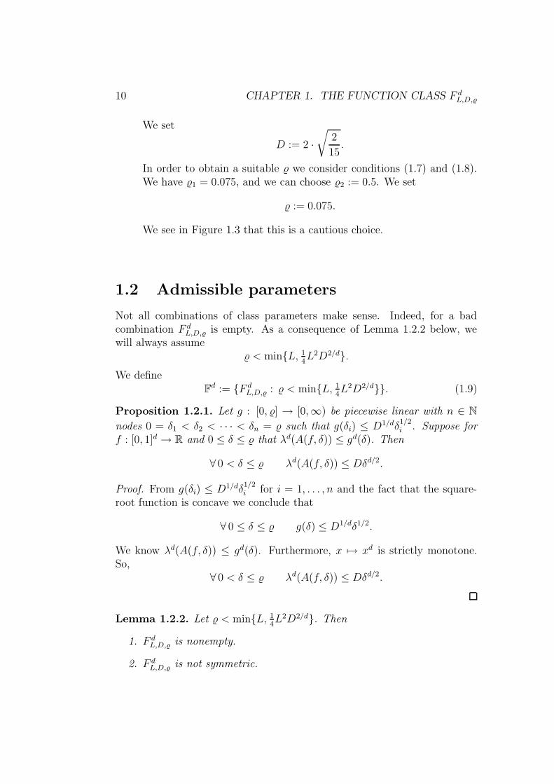
Figure 1.3: The function g3 and its level set function. The dashed lines areg and its level set function.
b) We guarantee A(f, %) ⊂ B(x∗, r, ‖ · ‖2): We set
% < %2 := inf|f(x) − f(x∗)| : x /∈ B(x∗, %1, ‖ · ‖2). (1.8)
For every % fulfilling conditions (1.7) and (1.8)
∀ 0 ≤ δ ≤ % λd(A(f, δ)) ≤ D δd/2
holds.
Example 1.1.3. Let g3 be the natural cubic spline interpolating thepoints
[0, 2], [0.4, 0], [0.8, 1], [1, 0.6],
see Figure 1.3. The global minimizer
x∗ =106
175− 2
√2846
525≈ 0.4025
has the function value g3(x∗) ≈ −0.00011269. For x ∈ [x∗−0.1, x∗+0.1]
we have g′′3(x) ≥ 15. So, for the quadratic function
g(x) :=15
2(x− x∗)2 + g3(x
∗)
we have g|[x∗−0.1,x∗+0.1] ≤ g3|[x∗−0.1,x∗+0.1]. For g the level set function iseasy to calculate:
λ1(A(g, δ)) ≤ 2 ·√
2
15δ1/2.
10 CHAPTER 1. THE FUNCTION CLASS F dL,D,%
We set
D := 2 ·√
2
15.
In order to obtain a suitable % we consider conditions (1.7) and (1.8).We have %1 = 0.075, and we can choose %2 := 0.5. We set
% := 0.075.
We see in Figure 1.3 that this is a cautious choice.
1.2 Admissible parameters
Not all combinations of class parameters make sense. Indeed, for a badcombination F d
L,D,% is empty. As a consequence of Lemma 1.2.2 below, wewill always assume
% < minL, 14L2D2/d.
We defineF
d := F dL,D,% : % < minL, 1
4L2D2/d. (1.9)
Proposition 1.2.1. Let g : [0, %] → [0,∞) be piecewise linear with n ∈ N
nodes 0 = δ1 < δ2 < · · · < δn = % such that g(δi) ≤ D1/dδ1/2i . Suppose for
f : [0, 1]d → R and 0 ≤ δ ≤ % that λd(A(f, δ)) ≤ gd(δ). Then
∀ 0 < δ ≤ % λd(A(f, δ)) ≤ Dδd/2.
Proof. From g(δi) ≤ D1/dδ1/2i for i = 1, . . . , n and the fact that the square-
root function is concave we conclude that
∀ 0 ≤ δ ≤ % g(δ) ≤ D1/dδ1/2.
We know λd(A(f, δ)) ≤ gd(δ). Furthermore, x 7→ xd is strictly monotone.So,
∀ 0 < δ ≤ % λd(A(f, δ)) ≤ Dδd/2.
Lemma 1.2.2. Let % < minL, 14L2D2/d. Then
1. F dL,D,% is nonempty.
2. F dL,D,% is not symmetric.

1.2. ADMISSIBLE PARAMETERS 11
3. F dL,D,% is not convex.
4. For every x ∈ [0, 1]d the class F dL,D,% contains several functions f with
f(x) = min f .
Proof. 1. Letf(x) := L ‖x‖∞.
Then for δ ≤ LA(f, δ) = [0, δL−1]d,
i.e., λd(A(f, δ)) = (δL−1)d. For δ ≤ L2D2/d it follows λd(A(f, δ)) ≤ D δd/2.
2. We choose γ ∈ (%, L) and define
fγ(x) :=
L ‖x‖∞, ‖x‖∞ ≤ γL−1,γ, ‖x‖∞ > γL−1.
Analogously to 1., we show fγ ∈ F dL,D,%. Furthermore,
λd(fγ ≥ γ) = λd(fγ = γ) ≥ (1 − γL−1)d > 0.
It holds −fγ 6∈ F dL,D,% since
λd(A(−fγ , 0)) ≥ (1 − γL−1)d > 0.
3. We chooses ∈ (max1/2, %/L, 1).
For
α := D%d/2 −( %L
)d
we have α > 0. We set
r := min
1 − s
2, α1/d, %1/2D1/d
, δ1 :=
r2
D2/d.
In particular,δ1 ≤ %.
For
fr,s(x) :=
δ1‖x‖∞r
, ‖x‖∞ ≤ r,
δ1 + L(‖x‖∞ − r), r < ‖x‖∞ ≤ s+ 1
2,
δ1 + L
(s+ 1
2− r
),s+ 1
2< ‖x‖∞ ≤ 1,

12 CHAPTER 1. THE FUNCTION CLASS F dL,D,%
0.2
0.4
0.6
0.8
0 0.2 0.6 0.8 10
0.40
0.2
0.4
0.6
0.8
1
1.2
0 0.2 0.4 0.6 0.8 1
Figure 1.4: The function fr,s and its level set function for d = 1, L = 1,D = 1, % = 1/9 and s = 3/4
we show fr,s ∈ F dL,D,%: Due to δ1 ≤ % < 1
4L2D2/d it holds
δ1r
=δ1/21
D1/d< 1
4L.
Consequently, the Lipschitz condition is fulfilled. For the level sets we have
λd(A(fr,s, δ)) =
(δr
δ1
)d
, δ ≤ δ1,(δ − δ1L
+ r
)d
, δ1 < δ < δ1 + L
(s+ 1
2− r
),
1, δ1 + L
(s+ 1
2− r
)≤ δ.
Consider the piece-wise linear function g with nodes and function values
g(0) = 0, g(δ1) = r, g(%) = (%− δ1)/L + r.
Application of Proposition 1.2.1 yields
∀ 0 < δ ≤ % λd(A(fr,s, δ)) ≤ D δd/2,
i.e., we showed fr,s ∈ F dL,D,%. In the same way, we prove
x 7→ fr,s( − x) ∈ F d
L,D,%,
with
:= (1, . . . , 1)T ∈ Rd.

1.2. ADMISSIBLE PARAMETERS 13
We consider the convex combination
g(x) := 12(fr,s(x) + fr,s(
− x)).
a) For x ∈ [0, 1]d let x := ‖x‖∞ · . For all x ∈ [0, 1]d the point x lies on the
diagonal t · , t ∈ [0, 1]. Furthermore, we have ‖x‖∞ = ‖x‖∞. So,
g(x) = 12(fr,s(x) + fr,s(
− x)) = 12(fr,s(x) + fr,s(
− x))
≥ 12(fr,s(x) + fr,s(
− x)) = g(x).
b) The function g is point symmetric in/2.
c) From x < y ≤ /2 we conclude g(x) ≤ g(y).
d) We have
g(0) = miny∈[0,1]d
g(y) = 12[δ1 + L((s + 1)/2 − r)].
e) It holds[0, r]d ∪ [1 − r, 1]d ⊂ A(g, δ1/2).
In conclusion,
λd(A(g, δ1)) ≥ λd(A(g, δ1/2)) ≥ 2 rd = 2D δd/21 > D δ
d/21 .
Since δ1 ≤ % we have g /∈ F dL,D,%.
4. We show that for every x ∈ [0, 1]d
fx(z) := L ‖z − x‖∞ ∈ F dL,D,%.
Obviously, the Lipschitz condition is fulfilled. For δ ≤ 14D2/dL2 we have
λd(A(fx, δ)) ≤ D δd/2.
(We have equality for x = 12·
and δ = 14D2/dL2.) Let θ > 0 be defined by
% = θ2
4D2/dL2. It holds θ ∈ (0, 1). We define
fx(z) := θL‖z − x‖∞.
We conclude fx ∈ F dθL,D,% ⊂ F d
L,D,%.
Remark 1.2.3. We showed that for % < min 14L2D2/d, L the problem class
F dL,D,% is neither convex nor symmetric. The problem class being not convex
or not symmetric is a necessary condition for the situation that adaptivemethods are essentially better than non-adaptive ones, see Section 3.2.


Chapter 2
Optimization algorithms
We propose two adaptive algorithms. The first one is applicable in a situationwhere the Lipschitz parameter L of the objective is known, or at least anupper bound of it. The second one is suitable for the case that the Lipschitzparameter is unknown. For both algorithms, the knowledge of the otherparameters D and % is unimportant for their definition and their success.Nevertheless, they are important for the cost estimation.
For both algorithms we give cost and error bounds according to the fol-lowing definitions:
The error of a method A applied to a function f and returningA(f) = x∗ = x∗(f) is given by
∆(A, f) := f(x∗) − inf f.
The (worst case) error of the method A is
∆(A, F dL,D,%) := sup ∆(A, f) : f ∈ F d
L,D,%.
The function-wise cost cost(A, f) of the method A applied to f is the numberof function calls the method A uses for f . The (worst case) cost of A is
cost(A, F dL,D,%) := sup cost(A, f) : f ∈ F d
L,D,%.
We come to some preliminaries for the two algorithms we propose. Lete(i) be the i-th unit vector in R
d having (e(i))i = 1 and (e(i))j = 0 for j 6= i.The algorithms use
Y (j) :=
d∑
i=1
aj · e(i), aj ∈ −3−j+1, 0, 3−j+1
\ 0, j ∈ N.
15

16 CHAPTER 2. OPTIMIZATION ALGORITHMS
Each of the sets Y (j) consists of 3d − 1 points. Finally, let
M := (12, . . . , 1
2)T
denote the midpoint of the unit cube in Rd.
2.1 The case of a known Lipschitz constant
For the case of a known Lipschitz parameter L, we propose the followingoptimization algorithm S(L, k) performing step(L, 1), . . . , step(L, k) asdescribed in Figure 2.1. After these k steps, S(L, k) returns x∗. It is similarto the one of Perevozchikov (1990).
Lemma 2.1.1. Let f : [0, 1]d → R be Lipschitz with constant L > 0. Afterstep(L, j) and for each global minimizer x∗ there exists a pair(xj, f(xj)) ∈ NL,j such that ‖xj − x∗‖∞ ≤ 2−13−j+1.
Proof. By induction.
j = 1: We have (M, f(M)) ∈ NL,1 and ‖x−M‖∞ ≤ 2−1 for all x ∈ [0, 1]d.
j → j + 1: Let (xj, f(xj)) ∈ NL,j such that ‖xj − x∗‖∞ ≤ 2−13−j+1. Instep(L, j + 1), we check whether f(xj) ≤ f∗ + L 2−13−j+1. This is true:
|f(xj) − f∗| ≤ |f(xj) − f(x∗)| ≤ L 2−13−j+1. (2.1)
So we choose the pairs
(xj + y, f(xj + y)), y ∈ Y (j + 1),
to be in NL,j+1. For (at least) one of these y we have
‖xj + y − x∗‖∞ ≤ 2−13−j.
Choose xj+1 := xj + y for such a y.
The sets NL,j are subsets of the equidistant meshes
mesh(j) :=
d∑
i=1
αi · e(i), αi ∈ 2−13−j+1 + l · 3−j+1, l = 0, . . . , 3j−1 − 1.
Furthermore, S(L, k) guarantees the same level of approximation as mesh(k)in the following sense: For every global minimizer x∗ we have
minx∈mesh(k)
‖x− x∗‖∞ ≤ 2−13−k+1, minx∈NL,k
‖x− x∗‖∞ ≤ 2−13−k+1.

2.1. THE CASE OF A KNOWN LIPSCHITZ CONSTANT 17
step(L, 1):
get f(M) (oracle call);
set NL,1 := (M, f(M));set x∗ := M; f∗ := f(M).
step(L, j ), 2 ≤ j ≤ k:
set NL,j := ∅;for (x, f(x)) ∈ NL,j−1 do
if (f(x) ≤ f∗ + L 2−13−j+2 ) then (∗)set NL,j := NL,j ∪ (x, f(x));for y ∈ Y (j) do
get f(x + y) (oracle call);
set NL,j := NL,j ∪ (x + y, f(x+ y));if (f(x+ y) < f∗) then
set x∗ := x+ y; f∗ := f(x+ y);
end if;
next y;
end if;
next x;
Figure 2.1: S(L, k) performs step(L, 1), . . . , step(L, k) and then returns x∗
We are now ready to prove cost and error bounds of S(L, k). We needthe following constants:
εL,k := L2−13−k+1, (2.2)
j(L, %) := dlog3(L/(2%))e + 3, (2.3)
j(L,D, %, d) := dlog3(L/(2%2D2/d))e + 6, (2.4)
c(d) :=3d/2
3d/2 − 1. (2.5)

18 CHAPTER 2. OPTIMIZATION ALGORITHMS
For d ≥ 1, we have c(d) ∈ (1, 2.37]. We use an idea of Perevozchikov(1990) to prove the following result.
Theorem 2.1.2. 1. Error estimation: For k ∈ N, we have
∆(S(L, k), F dL,D,%) ≤ εL,k.
2. Cost estimation: We have
(a) for k ∈ N
cost(S(L, k), F dL,D,%) ≤ 3d(k−1),
(b) for k ≥ j(L, %)
cost(S(L, k), F dL,D,%)
≤(
272L/%
)d+ c(d) (3d − 1)DLd/22−d/2
(3(k−1)d/2 −
(32L/%
)d/2),
(c) for k ≥ maxj(L, %), j(L,D, %, d)
cost(S(L, k), F dL,D,%) ≤ DLd/22−d/23(k+1)d/2+1 = DLd2−d3d+1ε
−d/2L,k .
Proof. 1. Let f ∈ F dL,D,%. From Lemma 2.1.1 we know that there exists a
pair (xk, f(xk)) ∈ NL,k such that ‖xk − x∗‖∞ ≤ 2−13−k+1. Then
|f(x∗) − f(x∗)| ≤ |f(xk) − f(x∗)| ≤ L 2−13−k+1.
2. For (a), we have that S(L, k) chooses only points in mesh(k), whichconsists of 3d(k−1) points.
(b). LetN∗
L,j−1 (2.6)
be the set of pairs (x, f(x)) ∈ NL,j−1 that in step(L, j) pass the testf(x) ≤ f∗ + L2−13−j+2. Then, in step(L, j), the number of new functionevaluations is bounded by
|NL,j \NL,j−1| ≤ (3d − 1)N∗j−1.
We can use this estimation for every step(L, j) with N ∗L,j−1 ⊂ A(f, %). As
in 1., we can show
min f(y) : y ∈ N ∗L,j−1 ≤ min f + L 2−13−j+2.
Furthermore,
∀x ∈ N∗L,j−1 f(x) ≤ f∗+L 2−13−j+2 ≤ min f(y) : y ∈ N ∗
L,j−1+L 2−13−j+2.
2.1. THE CASE OF A KNOWN LIPSCHITZ CONSTANT 19
So we get∀x ∈ N∗
L,j−1 x ∈ A(L 3−j+2).
For x, y ∈ N∗L,j−1 and x 6= y we have
B(x, 2−13−j+2) ⊂ A(L 2−13−j+3), B(x, 2−13−j+2) ∩ B(y, 2−13−j+2) = ∅.
For L 2−13−j+3 ≤ %, i.e.,
j − 1 ≥ dlog3(L/(2%))e + 2 = j(L, %) − 1,
we can estimate
|N∗L,j−1 | ≤ λd(A(L 2−13−j+3))
λd(B(x, 123−j+2))
≤ D (L 2−13−j+3)d/2
(3−j+2)d
= DLd/22−d/23(j−1)d/2 . (2.7)
So the number of new points in level j is bounded by
(3d − 1)DLd/22−d/23(j−1)d/2.
It follows immediately that
cost(S(L, k), F dL,D,%)
≤ |mesh(j(L, %) − 1)| +k∑
j=j(L,%)
(3d − 1)DLd/22−d/23(j−1)d/2
≤(
272L/%
)d+ c(d) (3d − 1)DLd/22−d/2(3(k−1)d/2 − 3(k(L,%)−2)d/2)
≤(
272L/%
)d+ c(d) (3d − 1)DLd/22−d/2
(3(k−1)d/2 −
(32L/%
)d/2).
So we proved (b).
Under the assumptions of (c) we have for d = 1
272L/% ≤ c(d)DL1/22−1/23(k−1)/2
and for d ≥ 2 (272L/%
)d ≤ 32· 3dDLd/22−d/23(k−1)d/2.
In both cases we conclude from (b) that
cost(S(L, k), F dL,D,%) ≤ DLd/22−d/23(k+1)d/2+1 = DLd2−d3d+1ε
−d/2L,k .
20 CHAPTER 2. OPTIMIZATION ALGORITHMS
2.2 The case of an unknown Lipschitz con-
stant
We now turn to the case of an unknown Lipschitz parameter L. For thissituation, we propose the algorithm Z as described in Figure 2.2. It uses thesteps of S(L, · ) for a sequence (L(i))i∈N of increasing Lipschitz constants.An additional step(L, 1’) is also used:
step(L, 1’):
oracle call: get f(M);
set NL,1 := (M, f(M)).
The constants L(i) and two controlling functions
lastconst : N → N, l 7→ lastconst(l)
laststep : N × N → N, (l, i) 7→ laststep(l, i)
determine the behavior of the algorithm. In a first definition, we only requirethe following properties:
• L(i+ 1) > L(i) for all i ∈ N,
• lastconst increasing,
• laststep(l, i) increasing in l, and decreasing in i.
Z(k) is a diagonal scheme. The parameter k in Z(k) is the number of per-formed diagonals. In diagonal l, the algorithm examines the objective assum-ing the Lipschitz constants L(1), . . . , L(lastconst(l)), i.e., for constant L(i),the algorithms performs
step(L(i), laststep(l − 1, i) + 1), . . . , step(L(i), laststep(l, i)).
While the algorithm has only one instance of f∗ and x∗, it uses separate setsNL(i),j for each constant L(i).Note that the objective f will be evaluated at certain points for severalconstants L(i), i.e., several times, the midpoint M for example lastconst(k)times. We will discuss in Section 2.2.1 why this is reasonable.

2.2. THE CASE OF AN UNKNOWN LIPSCHITZ CONSTANT 21
return x∗;
next l;
next i;
next j;
end if;
apply step(L(i), j );
else
apply step(L(i), 1’);
if (i 6= 1, j = 1) then
for j from 1 to laststep(l, i) do # step j
for i from 1 to lastconst(l) # constant L(i)
for l from 1 to k do # diagonal l
Figure 2.2: The algorithm Z(k). It uses the steps defined in Figure 2.1.
Let m, k ∈ N such that lastconst(k) ≥ m. The method Z(k) performsstep(L(m), 1’) (or 1) to step(L(m), laststep(k,m)). This way, Z(k) deter-mines the sets
NL(m),1, . . . , NL(m),laststep(k,m).
We have the following analogue to Lemma 2.1.1:
Lemma 2.2.1. Let f ∈ F dL,D,% with L ≤ L(m) for some m ∈ N, and
k ∈ N such that lastconst(k) ≥ m. Let x∗ be a global minimizer. For1 ≤ j ≤ laststep(k,m) there exists a pair (xj, f(xj)) ∈ NL(m),j such that‖xj − x∗‖∞ ≤ 2−13−j+1.
Proof. The proof is similar to that of Lemma 2.1.1. The only differencein the situation is that now, the least value found so far f∗ is shared andaltered by function evaluations applying different constants L(i). However,f∗ enters the proof only in (2.1). Here, f(x∗) ≤ f∗ ≤ f(xj) is needed. Thisis also true for the new situation. 2

22 CHAPTER 2. OPTIMIZATION ALGORITHMS
L(1) L(2) L(3) L(4)
step(L(i), 11)
step(L(i), 10)
step(L(i), 9)
step(L(i), 8)
step(L(i), 7)
step(L(i), 6)
step(L(i), 5)
step(L(i), 4)
step(L(i), 3)
step(L(i), 2)
step(L(i), 1)
const.step
1
2
3
4
5
6
7
8
9
10
11
12
13
14
15
16
17
18
19
20
21
22
k
k
k
k
k
k
k
k
k
k
k
k
k
k
k
k
k
k
k
k
k k
?
?
?7
7
7
7
7
7
7
7
7
7
7
7
Figure 2.3: Scheme of Z(h, k) for h = 3 and k = 10
We want to examine Z(k) for the choice
L(i) := 3i−1, i ∈ N, (2.8)
lastconst(l) :=
⌈l
h
⌉, laststep(l, i) :=
l − h(i− 1), if i ≤ lastconst(l),0, else,
with parameter h ∈ 3, 4, . . . and the ceiling function
d · e : R → Z, dre := infz ∈ Z : z ≥ r. (2.9)
We will discuss the choice of h in Remark 2.2.3 and in Chapter 4. Let
Z(h, k)

2.2. THE CASE OF AN UNKNOWN LIPSCHITZ CONSTANT 23
be the algorithm defined in this manner. We use the constants
εL,h,k := Lh+12−13−k+1, (2.10)
c(d, h) :=1
1 − 3−hd/2, c′(d, h) :=
1
1 − 3(1−h/2)d, (2.11)
C(L, d, h) := c(d)[c(d, h)3−d/2 + c′(d, h)L−hd/2
], (2.12)
with c(d) defined as in (2.5). For h ≥ 3, d ≥ 1, and L ≥ 1 we have
c(d, h) ∈ (1, 1.25], c′(d, h) ∈ (1, 2.37], C(L, d, h) ∈ (0, 7.37].
Theorem 2.2.2. Let m ∈ N and k ≥ h(m− 1) + 1.
1. Error estimation:
∆(Z(h, k), F dL(m),D,%) ≤ εL(m),h,k.
2. Cost estimation:
cost(Z(h, k), F dL(m),D,%)
≤(3Lh+1(m)/%
)dc(2d, h) + c(2d) 3d(dk/he−m)
(272L(m)/%
)d+
C(L(m), d, h)L(m)(h+1)d/2D 2−d/23(k−1)d/2
=(3Lh+1(m)/%
)dc(2d, h) +
(272L(m)/%
)dc(2d) 2−d/hL(m)d/h ε
−d/hL(m),h,k +
C(L(m), d, h)DL(m)(h+1)d2−d ε−d/2L(m),h,k.
Proof. 1. Let us assume that we apply Z(h, k) to a function f ∈ F dL(m),D,%.
For the constant L(m) our method performs step(L(m), 1) or step(L(m), 1’)up to step(L(m), k − h(m− 1)). From Lemma 2.2.1 we know that for everyglobal minimizer x∗ there exists xk−h(m−1) ∈ NL(m),k−h(m−1) such that
‖xk−h(m−1) − x∗‖∞ ≤ 2−13−k+h(m−1)+1.
It follows immediately that
|f(x∗)− f(x∗)| ≤ |f(xk−h(m−1))− f(x∗)| ≤ L(m) 2−13−k+h(m−1)+1 = εL(m),h,k.
2. The cost estimation is similar to the one in the proof of Theorem 2.1.2.Recall N∗
L,j−1 to be defined as in (2.6). We consider the steps for constants

24 CHAPTER 2. OPTIMIZATION ALGORITHMS
L ≥ L(m) and those for constants L < L(m) separately.
Let m ≤ i ≤ lastconst(k). For the new points in step(L(i), j ), we have
|NL(i),j \NL(i),j−1| ≤ (3d − 1)|N∗L(i),j−1|.
We can use this estimation for all j with N ∗L(i),j−1 ⊂ A(f, %). As in 1., we
can show
min f(y) : y ∈ NL(i),j−1 ≤ min f + L(m) 2−13−j+2.
Furthermore,
∀ x ∈ N∗L(i),j−1 f(x) < min f(y) : y ∈ NL(i),j−1 + L(i) 2−13−j+2,
so we get
∀ x ∈ N∗L(i),j−1 x ∈ A(f, (L(m) + L(i))2−13−j+2).
For x, y ∈ N∗L(i),j−1 with x 6= y we have
B(x, 2−13−j+2) ⊂ A(f, (2L(m) + L(i)) 2−13−j+2),
B(x, 2−13−j+2) ∩ B(y, 2−13−j+2) = ∅.
For (2L(m) + L(i))2−13−j+2 ≤ %, i.e.,
j − 1 ≥ dlog3((2L(m) + L(i))/(2%))e + 1 =: j(m, i, %) − 1, (2.13)
we get
|N∗L(i),j−1| ≤ λd(A(f, (2L(m) + L(i))2−13−j+2))
λd(B(x, 2−13−j+2))(2.14)
≤ D(L(m) + 2−1L(i))d/2 3(j−2)d/2.
It follows immediately that
|NL(i),j \NL(i),j−1| ≤ (3d − 1)D(L(m) + 2−1L(i))d/2 3(j−2)d/2.
2.2. THE CASE OF AN UNKNOWN LIPSCHITZ CONSTANT 25
For k − h(i− 1) ≥ j(m, i, %) we get the cost estimation
|NL(i),1| +k−h(i−1)∑
j=2
|NL(i),j \NL(i),j−1|
≤ |mesh(j(m, i, %) − 1) | +k−h(i−1)∑
j=j(m,i,%)
(3d − 1)D(L(m) + 2−1L(i))d/2 3(j−2)d/2
≤(
9(2L(m) + L(i))
2%
)d
+
(3d − 1)D(L(m) + 2−1L(i))d/23(j(m,i,%)−2)d/2 3(k−h(i−1)−j(m,i,%)+1)d/2 − 1
3d/2 − 1
≤(
27L(i)
2%
)d
+ (3d − 1)DL(i)d/2c(d) 2−d/23(k−h(i−1)−1)d/2.
Now let 1 ≤ i ≤ m − 1. Again, we want to estimate |N ∗L(i),j−1|. Be-
fore the algorithm applies step(L(i), j), the last step concerning L(m) wasstep(L(m), j−1−h(m−i)). So we know that at the beginning of step(L(i), j)
f∗ ≤ min f + L(m)2−13−j+h(m−i)+2.
Consequently,
∀x ∈ N∗L(i),j−1 f(x) ≤ min f + 2−13−j+2[L(i) + L(m) 3h(m−i)].
Define
j ′(m, i, h, %) := dlog3((L(i) + L(m)(1 + Lh(m)/Lh(i)))/(2%))e + 2. (2.15)
We have j ′(m, i, h, %) ≤ h(m − i) + m + 1 − blog3(%)c. If k ≥ hm + 1 thenk − h(i − 1) ≥ j ′(m, i, h, %). In the same manner as above we can show forj ≥ j ′(m, i, h, %) that
|N∗L(i),j−1| ≤ λd(A(f, 3−j+2L(m)3h(m−i)))
λd(B(x, 2−13−j+2))
≤ DL(m)d/23(j+h(m−i)−2)d/2.

26 CHAPTER 2. OPTIMIZATION ALGORITHMS
We conclude that
|NL(i),1| +k−h(i−1)∑
j=2
|NL(i),j \NL(i),j−1|
≤ |mesh(j ′(m, i, h, %) − 1)| +k−h(i−1)∑
j=j′(m,i,h,%)
(3d − 1)DL(m)d/23(j+h(m−i)−2)d/2
≤(
3Lh+1(m)
Lh(i)%
)d
+ (3d − 1)DL(m)d/2c(d)3(k+h(m−2i+1)−2)d/2.
In order to get an estimation for cost(Z(h, k), F dL(m),D,%), we sum up these
numbers for the constants L(1), . . . , L(dk/he):
cost(Z(h, k), F dL(m),D,%) ≤
dk/he∑
i=1
|NL(i),1| +
k−h(i−1)∑
j=2
|NL(i),j \NL(i),j−1|
≤m−1∑
i=1
(3Lh+1(m)
Lh(i)%
)d
+
dk/he∑
i=m
(9(3L(i))
2%
)d
+
m−1∑
i=1
(3d − 1)DL(m)d/2c(d)3(k+h(m−2i+1)−2)d/2 +
dk/he∑
i=m
(3d − 1)DL(i)d/2c(d)2−d/23(k−h(i−1)−1)d/2
≤(3Lh+1(m)/%
)d m−2∑
i=0
3−hdi +
(27
2
L(m)
%
)d dk/he−m∑
i=0
3di +
(3d − 1)DL(m)d/2c(d)3(k+h(m−1)−2)d/2
m−2∑
i=0
3−dhi +
(3d − 1)DL(m)d/2c(d)2−d/23(k−h(m−1)−1)d/2
dk/he−m∑
i=0
3(1−h/2)di (2.16)
≤(3Lh+1(m)/%
)dc(2d, h) + c(2d) 3d(dk/he−m)
(272L(m)/%
)d+
(3d − 1)DL(m)d/2c(d) c(2d, h) 3(k+h(m−1)−2)d/2 +
(3d − 1)DL(m)d/2c(d)2−d/23(k−h(m−1)−1)d/2c′(d, h)
≤(3Lh+1(m)/%
)dc(2d, h) + c(2d) 3d(dk/he−m)
(272L(m)/%
)d+
(3d − 1)DL(m)d/2c(d)3(k−1+h(m−1))d/2[c(2d, h)3−d/2 + c′(d, h)2−d/23−(m−1)hd
]

2.2. THE CASE OF AN UNKNOWN LIPSCHITZ CONSTANT 27
≤(3Lh+1(m)/%
)dc(2d, h) + c(2d) 3d(dk/he−m)
(272L(m)/%
)d+
C(L(m), d, h)L(m)(h+1)d/2D 2−d/23(k−1)d/2.
With
ε−d/2L(m),h,k = L(m)−(h+1)d/22d/23(k−1)d/2, ε
−d/hL(m),h,k = L(m)−d−d/h2d/h3d(k−1)/h,
we get
cost(Z(h, k), F dL(m),D,%)
≤(3Lh+1(m)/%
)dc(2d, h) +
(272L(m)/%
)dc(2d) 2−d/hL(m)d/h ε
−d/hL(m),h,k +
C(L(m), d, h)DL(m)(h+1)d2−d ε−d/2L(m),h,k.
Remark 2.2.3. We can now explain the restriction on the parameter h: Inorder for the sum in (2.16) to be bounded for all k ∈ N, we need h ≥ 3.The parameter h allows us to decide whether to focus on local or on globalsearch in the following sense: The cost used by performing the steps for L(i)with i ≥ m are approximately
(3d − 1)DL(i)d/2c(d) 2−d/23(k−h(i−1)−1)d/2.
For constant L(i + 1) we spend 3−(h−1)d/2 times as much as we spend forL(i). Choosing a high value for h leads to focus on a precise approximationof found (local) minima. This is done in steps for small constants L(i). Onthe other hand, a low value of h, of say, 3 or 4, will focus more on globalsearch, performed by steps for big constants L(i).
We will give an heuristic advice on how to choose h in Chapter 4.
We close the examinations in this section by showing that (Z(k)(f))k∈N
converges for every continuous f .
Lemma 2.2.4. Let f ∈ C[0, 1]d. Then
limk→∞
f((Z(k)(f))) = inf f.
Proof. Since f is continuous, it is sufficient to show that
∀j ∈ N ∀x ∈ mesh(j) ∃ k ∈ N Z(k) evaluates at x.
Let M := sup |f | and L := 4M3j−2. For L ≥ L we show by induction
∀ 1 ≤ l ≤ j ∀x ∈ mesh(l) (x, f(x)) ∈ NL,l.

28 CHAPTER 2. OPTIMIZATION ALGORITHMS
l = 1 is obvious.l − 1 → l for 2 ≤ l ≤ j: Let x ∈ mesh(l − 1). Under the assumption of theinduction, we have (x, f(x)) ∈ NL,l−1. Furthermore,
|f(x) − f∗| ≤ 2M = L2−13−j+2 ≤ L2−13−l+2.
So for all y ∈ Y (l) ∪ 0 we have
(x+ y, f(x+ y)) ∈ NL,l.
Now let i ∈ N such that L(i) ≥ L, and k ∈ N such that lastconst(k) ≥ i andlaststep(k, i) ≥ j. Then Z(k) evaluates f at every x ∈ mesh(j).
2.2.1 A remark on computational cost and on storage
requirements
The cost definition we use is limited to the information cost, i.e., the numberof function calls the method uses. However, the development of arithmeticcost and storage requirements are important for implementation, too. Wewill sketch that for the first and the second algorithm our cost definition isa good measure also for these quantities. This is not obvious. In fact, thepolicy of the second algorithm not to store every function value is necessaryto obtain this result.
We examine the arithmetic cost and storage requirements for the algo-rithm Z(h, k), then ask how much the (information) cost bound could beimproved if we stored all function values, and then reconsider the arithmeticcost for this case. A similar argumentation applies for the simpler situationof the first algorithm.
Arithmetic cost and storage requirements for Z(h, k)
We start with the arithmetic cost. We reconsider Figure 2.2. We neglectthe arithmetic cost necessary for the three “for”-loops and the “if”-loop.So we must still consider the steps(L, j) as in Figure 2.1, and step(L, 1′) ason page 20. For step(L, 1) and step(L, 1′) we have one oracle call, i.e., theinformation cost is 1. On the other hand, the arithmetic cost is bounded bya constant. In step(L, j) with j ≥ 2, we have to run an outer “for”- and an“if”-loop for every point (x, f(x)) ∈ NL,j−1 . The effort to run these loops isbounded by a fixed constant times the information cost of step(L, j−1). Thecost of the inner “for”-loop is bounded by a constant times the informationcost of step(L, j). Altogether, the arithmetic cost behaves linearly to theinformation cost.

2.2. THE CASE OF AN UNKNOWN LIPSCHITZ CONSTANT 29
We turn to the storage requirements. We neglect the storage of x∗, f∗, andthe variables needed to run the “for”-loops and the “if”-loop. The storage re-quirements for the sets NL,j remain to be considered. The information cost isan upper bound for their storage requirements since for every (x, f(x)) ∈ NL,j
there has been an oracle call at x, and if (x, f(x)) is stored several times,l times say, then x has also been evaluated (at least) l times.
Possible information cost reduction
We want to find out how much (information) cost we may save if we storeall function evaluations and evaluate at the same point only once.
Proposition 2.2.5. Let f : [0, 1]d → R be Lipschitz with constant L > 0.
For L ≥ 3L we have
∀ j ∈ N NL,j ⊂ NeL,j .
Proof. We show
∃j ∈ N NL,j 6⊂ NeL,j ⇒ ∃ x1, x2 ∈ [0, 1]d |f(x1) − f(x2)| > L‖x1 − x2‖∞.
Let x ∈ NL,j but x 6∈ NeL,j. From x ∈ NL,j we conclude that there exists ay ∈ NL,j−1 with
f(y) ≤ minf(z) : z ∈ NL,j−1 + L 2−13−j+2, ‖ y − x ‖∞ ≤ 3−j+1.
Since x 6∈ NeL,j we conclude for this y that
f(y) > minf(z) : z ∈ NeL,j−1 + L 2−13−j+2.
Consequently,
minf(z) : z ∈ NeL,j−1 < minf(z) : z ∈ NL,j−1 − (L− L)2−13−j+2
︸ ︷︷ ︸=L 3−j+2
.
So,
inf f < minf(z) : z ∈ NL,j−1 − L 3−j+2,
which is a contradiction to Lemma 2.1.1.
It is easy to see that a similar result for a Lipschitz constant L < L cannothold. However, we can use Proposition 2.2.5 to improve the cost bound of

30 CHAPTER 2. OPTIMIZATION ALGORITHMS
Theorem 2.2.2. Again, we assume f ∈ F dL(m),D,%. For Lipschitz constants
L(i) with m ≤ i ≤ lastconst(k) we only have to consider the cost
k−h(i−1)∑
j=k−hi+1
|NL(i),j \NL(i),j−1|
≤ (3d − 1)DL(i)d/2c(d)2−d/23(k−h(i−1)−2)d/2
if k− hi+ 1 ≥ j(m, i, %). We compare this with the corresponding cost as inthe proof of Theorem 2.2.2:
|NL(i),1| +k−h(i−1)∑
j=2
|NL(i),j \NL(i),j−1|
≤(
27L(i)
2%
)d
+ (3d − 1)DL(i)d/2c(d) 2−d/23(k−h(i−1)−1)d/2.
We save the cost of(
27L(i)2%
)d
, which belongs to the less important part of
the cost estimation. For the important one, we reduce the cost by the fac-tor 3−d/2. This is a good improvement, especially for higher dimensions.However, we cannot improve the rate of convergence. Furthermore, this im-provement is restricted to only a part of the cost estimation. The cost boundfor constants L(i) < L(m) and L(i) = L(lastconst(k)) stays the same.
Arithmetic cost revisited
We still assume that we store all function evaluations. Evaluating only onceat the same point means that for every function value that we need duringa step(L(i), j) with i ≥ 2, we first check whether it was already determinedand then, in case it was not, perform an oracle call.
Let us assume that we already evaluated at n points and that we mustnow ask whether a certain point has already been evaluated. If we do notsort the evaluation points then we need to assume a worst-case cost of O(n).We conclude for the whole checking procedure that after n function calls wehave a total arithmetic cost of order O(n2).
We are in a better situation if we sort. It is well-known that the bestsorting routines can reduce the arithmetic cost for the complete sorting pro-cedure to O(n · logn). In this case, an additonal logarithmic factor must stillbe considered, i.e., even when sorting, the information cost is no longer agood measure for the arithmetic cost.
For the above reason, we decided not to store all function evaluations.

2.2. THE CASE OF AN UNKNOWN LIPSCHITZ CONSTANT 31
Remark 2.2.6. We have only been vague about the definition of the arith-metic cost. It will be treated in detail in Section 3.1. However, the aboveargumentation, which uses an intuitive understanding, is consistent with thedefinition that follows.

Chapter 3
Optimality results
We prove lower error bounds for adaptive deterministic, non-adaptive deter-ministic and adaptive randomized methods showing that
• the algorithms S(L, ·) and Z(h, ·) have the optimal rate of convergence,
• adaptiveness is essential for optimality and yields a quadratic speed-up,
• up to constants, randomization (Monte Carlo) gives no further advan-tage.
We also show that our second algorithm is universal for Fd as defined in
(1.9). Our first method has the optimal rate of convergence if the Lipschitzconstant is known.
We start with some important concepts.
3.1 The concept of Information-Based Com-
plexity
Let F be a problem class of real valued and bounded functions with a commondomain D ⊂ R
d. For some classes F every function f ∈ F can be describedwith a finite number of parameters. This is the case, e.g., for classes ofpolynomials x 7→ anx
n + · · · + a0. However, for many interesting classes,and also for F d
L,D,%, this is not the case. In consequence, we cannot assumeto have a closed formula for every f ∈ F . This means in particular that fcannot be involved completely into the computation.
Instead, we assume that we have access to a finite number of functionvalues provided by a subroutine, the oracle. The computation itself is donewith the Unlimited Register Machine with an Oracle, a model of an idealized
33

34 CHAPTER 3. OPTIMALITY RESULTS
computer. In particular, we assume that we can calculate with real numbersand that we can store them.
3.1.1 The Unlimited Register Machine with an Oracle
Our model of computation is the Unlimited Register Machine (URM) withan Oracle. We follow the approach of Novak (1995), but add the ceilingfunction to the allowed artihmetic instructions. We do not mention whathappens if an error occurs, e.g., if we divide by zero or if the program doesnot terminate. For those cases and to learn more about the URM we referto Novak (1995).
For every k ∈ Z we have a register Rk with an entry rk which is a realnumber. At the beginning of the computation we have rk = 0 for all k ∈ Z.The contents of the registers may be altered by the machine in responseto certain instructions. An algorithm is a finite list of instructions. Afterthe machine has worked off this list and if d := r0 ∈ N then the outputis the vector (r1, . . . , rd). For the global optimization problem, the outputis interpreted as the coordinates of the approximation x∗. The followinginstructions can be used:
Arithmetic instructions
• Addition of a constant. For i ∈ Z and s ∈ R there is an instructionAdd(i, s). The response of the machine is ri := ri + s.
• Addition of two numbers. For i, j, k ∈ Z there is an instructionAdd(i, j, k). The response of the machine is ri := rj + rk.
• Multiplication with a constant. For i ∈ Z and s ∈ R there is aninstruction Mul(i, s). The response of the machine is ri := ri · s.
• Multiplication of two numbers. For i, j, k ∈ Z there is an instructionMul(i, j, k). The response of the machine is ri := rj · rk.
• Division of two numbers. For i, j, k ∈ Z there is an instructionDiv(i, j, k). The response of the machine is ri := rj/rk.
• Ceiling operation. For i ∈ Z there is an operation Ceil(i). The responseof the machine is ri := drie, where d · e is defined as in (2.9).

3.1. THE CONCEPT OF INFORMATION-BASED COMPLEXITY 35
Jump instruction
• For i, j ∈ Z and l ∈ N there is an instruction Jump(i, j, l). Ifri ≥ rj then the machine proceeds with the next instruction of thelist, otherwise it proceeds with the l-th instruction of the list.
Copy instructions
• Assignment of a constant. For i ∈ Z and s ∈ R there is an instructionAssign(i, s). The response of the machine is ri := s.
• Direct and indirect copy assignments. For i, l ∈ Z there are four differ-ent kinds of direct and indirect copy instructions Copy(i, l), Copy(ri, l),Copy(i, rl), Copy(ri, rl). The response of the machine to Copy(ri, rl) isrri
:= rrlif ri, rl ∈ Z. The response of the other instructions is defined
analogously.
Oracle call
• For i ∈ Z there is an instruction Oracle(i). The response of the machineis as follows. Let d := r−1 and f ∈ F be the problem element. If d ∈ N
and f(r−2, . . . , r−d−1) is defined, then the response of the machine isri := f(r−2, . . . , r−d−1).
This list of available instructions could be completed by other computationsone may wish to perform. For example, one may wish to have instructionsthat calculate the functions sin, cos, exp eliminating the need to worry aboutapproximation errors. In Section 5.2 we present a variant of our universalalgorithm, which also uses the function x 7→ xα for some α ∈ (0, 1/2). Here,we wish to add an instruction to our list delivering this calculation.
Definition 3.1.1. A finite list of instructions for the URM with an Oracleis called an algorithm if for all f ∈ F no error occurs, i.e., if all instructionsare used only with admissible parameters, if the calculation terminates, andif in the final configuration r0 is equal to the dimension d of the domain Dand (r1, . . . , rd)
T ∈ D.
Synonymously, we also call an algorithm a method.
Example 3.1.2. We present a simple optimization algorithm for univaritatefunctions defined on [0, 1]. The program uses the oracle to get the functionvalues for 1/6, 1/2, 5/6 and then returns the (smallest) point with the leastfunction value.

36 CHAPTER 3. OPTIMALITY RESULTS
1. Assign(−1, 1) 8. Assign(1, 5/6)2. Assign(−2, 1/6) 9. Jump(4, 3, 12)3. Oracle(2) 10. Assign(1, 1/2)4. Assign(−2, 1/2) 11. Copy(4, 3)5. Oracle(3) 12. Jump(4, 2, 14)6. Assign(−2, 5/6) 13. Assign(1, 1/6)7. Oracle(4) 14. Assign(0, 1)
We see that even for this straightforward example, an algorithm writtenin the language of the URM is rather hard to read. We introduced theURM to define the class of algorithms we want to consider. It is also anecessary requirement to define the notion of cost, especially computationalcost. However, we will also use other ways to describe algorithms – as wealready did for the algorithms of Chapter 2. The algorithm of Example 3.1.2can also be described by
f 7→ minargminf(1/6), f(1/2), f(5/6).
More generally, we can say that each algorithm A, as defined for the URM,induces a mapping on F , the one that maps f to the output A(f) of Aapplied to f . We call this mapping A, too.
Definition 3.1.1 allows an algorithm to use function values at adaptivelychosen points x(1), . . . , x(n). However, the first point x(1) is independent ofthe objective f and fixed for a particular algorithm. The points x(j) withj ≥ 2 may depend on those previously chosen and their function values.Also, the number of oracle calls may depend on the observed data. Everysuch method A can be expressed by
A(f) = φ N(f).
The information operator
N : F →∞⋃
n=1
Rn (3.1)
gives the function values at the adaptively chosen points. They are obtainedby applying functions ψj : R
j−1 → D such that
x(j) = ψj(f(x(1)), . . . , f(x(j−1))).
It stops after n oracle calls according to a stopping rule s :⋃∞
j=1 Rj → 0, 1
iff
∀j < n s(f(x(1)), . . . , f(x(j))) = 1, s(f(x(1)), . . . , f(x(n))) = 0.

3.1. THE CONCEPT OF INFORMATION-BASED COMPLEXITY 37
The mapping
φ :
∞⋃
i=1
Rn → D
constructs the output x∗ = x∗(f) = A(f) using the information vector N(f).This alternative notion of an algorithm is much more convenient for our
purposes to prove cost and error bounds, as we will see in the next section.
3.1.2 Cost and error
We distinguish between computational cost and information cost. For thecomputational cost we consider all instructions in the list of Section 3.1.1,except for the oracle call. It is generally assumed that the URM alwaysperforms a certain instruction at the same cost, i.e., that the cost of aninstruction does not depend on the arguments it is called with or the timewhen it is performed. In principle, it is possible to assign a different cost toevery type of instruction. Novak (1995) suggests assigning each arithmeticoperation and each jump unitary cost while a copy instruction is free. Forthe information cost, he prices every oracle call with c > 0. This constant isto be chosen in such a way that the cost of an arithmetic operation and thatof an oracle call are in an appropriate ratio. This ratio may depend on theparticular situation.
The cost approach we use is much simpler. We say that an oracle call hasunitary cost while all other instructions are free, i.e., we concentrate on theinformation cost. So,
cost(A, F )
is the number of oracle calls A needs to return an approximation A(f) forf ∈ F in the worst case. In Section 2.2.1 we showed that for our twoalgorithms this cost definition is also a good measure for arithmetic cost andstorage requirements, i.e., this simplification of the cost definition means onlya minor loss of information of how expensive an implementation is.
We come to the notion of the error. Let A be an optimization algorithm.For an element f of the problem class F we define the function-wise error
∆(A, f) := f(A(f)) − inf f.
The worst-case error of A is given by
∆(A, F ) := supf∈F
∆(A, f).
In Section 3.2 we will also give the notion of mean errors and errors of ran-domized methods.

38 CHAPTER 3. OPTIMALITY RESULTS
Example 3.1.3. We consider the problem class
FL := f : [0, 1] → R, |f(x) − f(y)| ≤ L|x− y| for all x, y ∈ [0, 1]
and the optimization algorithm An that evaluates f at the points
x(i) :=1
2n+i− 1
n, 1 ≤ i ≤ n,
and then returns A(f) which is the (smallest) point x(i) with the least ob-served function value.
Let f ∈ FL and x∗ ∈ [0, 1] be a global minimizer. Since the points x(i)
are chosen equidistantly, we can say
∃ j ∈ 1, . . . , n | x∗ − x(j) | ≤ 1
2n.
Using the Lipschitz property we get
f(A(f)) − f(x∗) ≤ f(x(j)) − f(x∗) ≤ L | x(j) − x∗ | ≤ L
2n.
So, ∆(An, f) ≤ L/(2n) and, since f ∈ F was arbitrary,
∆(An, F ) ≤ L/(2n).
3.1.3 Error numbers
We define error numbers for two classes of algorithms depending on thestructure of the information vector N as defined in (3.1). We say that analgorithm is adaptive if it fulfills Definition 3.1.1. It is non-adaptive if itadditionally fulfills
∃n ∈ N ∃ x1, . . . , xn ∈ [0, 1]d ∀f ∈ F dL,D,% N(f) = (f(x1), . . . , f(xn)).
Note that non-adaptive algorithms are a sub-class of adaptive algorithms.From a practical point of view, non-adaptive methods are advantageous
in that the function values f(x(i)) can be determined parallelly. On the otherhand, adaptive methods often need far less function calls.
We sayA ∈ Aad
n (F )
if A is adaptive and has cost(A, F ) ≤ n, and
A ∈ Anonn (F )

3.1. THE CONCEPT OF INFORMATION-BASED COMPLEXITY 39
if A is non-adaptive with cost(A, F ) ≤ n. We have Anonn (F ) ⊂ Aad
n (F ). Wedefine the error numbers
eadn (F ) := inf ∆(A, F ) : A ∈ Aadn (F ), (3.2)
enonn (F ) := inf ∆(A, F ) : A ∈ Anon
n (F ). (3.3)
The error numbers eadn (F ) give information about the intrinsic difficulty ofthe optimization problem. Any method yielding an error of at most eadn (F )for all f ∈ F uses at least n function calls for at least one function f ∈ F .These error numbers are the benchmark for our algorithms. Furthermore, wesay that adaptive algorithms are essentially better than non-adaptive ones if
limn→∞
eadn (F )
enonn (F )
= 0.
Example 3.1.4. We reconsider the class FL of Example 3.1.3. Since for theparticular non-adaptive algorithm An we could prove ∆(An, FL) ≤ L/(2n),we conclude that
eadn (FL) ≤ enonn (FL) ≤ L
2n.
For a lower bound we consider an arbitrary (adaptive) algorithm A that usesat most n function values. We can assume that A uses exactly n functionvalues. Let x(1), . . . , x(n) be the points chosen by the algorithm for the func-tion h(x) ≡ 0 and x(n+1) := A(h). Without loss of generality, we assumex(1) ≤ · · · ≤ x(n+1). There exists at least one point z ∈ [0, 1] such that
min1≤i≤n+1
|z − x(i)| ≥ 1
2(n+ 1).
We define the function
gz(x) :=
− L2(n+1)
+ L|z − x|, x ∈ [z − 1/(2(n+ 1)), z + 1/(2(n+ 1))],
0, else.
We easily check gz ∈ FL and A(gz) = A(h) = x(n+1). So,
gz(A(gz)) = 0, min gz = − L
2(n+ 1).
We have ∆(A, gz) = L/(2(n + 1)). Consequently, ∆(A, FL) ≥ L/(2(n + 1)),such that
L
2(n+ 1)≤ eadn (FL) ≤ enon
n (FL) ≤ L
2n.
With some more effort, one can show that L/(2n) ≤ eadn (FL), see Novak(1988), Proposition 1.3.6, for details. This means that for FL non-adaptivemethods are optimal. We will see in the next section that this is no coinci-dence.
40 CHAPTER 3. OPTIMALITY RESULTS
We will also introduce error numbers for mean errors and for randomizedmethods in Section 3.2.
3.1.4 Universality and tractablilty
We introduce two important notions.
Definition 3.1.5. Let F be a family of problem classes and (An)n∈N be asequence of optimization algorithms with cost(An, F ) ≤ n for every F ∈ F .The methods An are called universal for F if
∀F ∈ F ∃CF <∞ ∀n ∈ N ∆(An, F ) ≤ CF · eadn (F ).
We also call a subsequence (An(i))i∈N universal for F if n(i) ↑ ∞.
Definition 3.1.6. Let (Fd)d∈N be a sequence of function classes. The globaloptimization problem is tractable for (Fd)d∈N if there exists an estimate ofthe sort
∀d, n ∈ N eadn (Fd) ≤ C · dp · n−q
with a constant C > 0 and p ≥ 0, q > 0, all independent of d and n. It isstrongly tractable if we can choose p = 0.
The general case is that one considers tractabilty concerning the dimen-sion of the domain.
3.2 Some known complexity results
A well examined optimization problem is convex programming. Here, wehave a unique global minimizer. Local and global search coincide. For thissituation methods are known whose costs behave polynomially in dimensiond and error level ε. This means in particular that convex programming istractable. The ellipsoid method assumes the existence of an oracle thatdelivers for a problem element f and a point x of the domain both thefunction value f(x) and the derivative (∇f)(x). It yields an approximationto the error level ε > 0 using O(d2 ln(1/ε)) oracle calls. For details andfurther complexity results for convex functions we refer to the mini-course ofNemirovski (1995).
The problem class F dL,D,% contains functions with many global minimizers.
In this property, it is closely related to Lipschitz classes. For
F dL := f : [0, 1]d → R, |f(x) − f(y)| ≤ L ‖x− y‖∞ for all x, y ∈ [0, 1]d,

3.2. SOME KNOWN COMPLEXITY RESULTS 41
we have that a non-adaptive method using equidistant points delivers theoptimal result. The class F d
L is a special case of a convex and symmetric(i.e., f ∈ F ⇒ −f ∈ F ) class. In this situation, adaptiveness can yieldonly a minor improvement, if at all, compared to the best non-adaptivealgorithms. See Novak (1988), Proposition 1.3.2, for details. On the otherhand, there are examples that adaptiveness helps essentially if the problemclass is convex but not symmetric or vice versa.
Let (an)n∈N and (bn)n∈N be non-negative sequences and 0 < c ≤ C < ∞such that
∃N ∈ N ∀n ≥ N c · an ≤ bn ≤ C · an.
Then we writean bn.
For F dL, we have e
ad/nonn (F d
L) Ln−1/d. In contrast, we will see for F dL,D,%
that adaption is essential for optimality and that it leads to a quadraticspeed-up: eadn (F d
L,D,%) L2D2/dn−2/d. In both cases, however, the errornumbers depend exponentially on d, which means that for F d
L and F dL,D,% the
optimization problem is not tractable.
One may say that in many situations the worst case definition of error orcost is too pessimistic and that the average case may give a more realisticpicture. Let F be a problem class endowed with a probability measure Pdefined on a suitable σ-algebra. The mean error of a method A is defined by
∆(A, P ) :=
∫
F
∆(A, f)P (df),
if the function-wise error ∆(A, f) is a measurable function. (If not, one mayapply the upper integral instead.) The mean error numbers for adaptive andnon-adaptive methods are given by
eadn (P ) := inf∆(A, P ) : A ∈ Aadn (F ), (3.4)
enonn (P ) := inf∆(A, P ) : A ∈ Anon
n (F ).A prominent model for d = 1 is to assume the Wiener measure P ∗ on C[0, 1].It is easy to see that for F = C[0, 1] the worst-case error of any methodA is unlimited. We have only little knowledge concerning the mean errornumbers. Ritter (1990), Theorem 4, proves the upper bound
∃C > 0 enonn (P ∗) ≤ C · n−1/2.
For a lower bound, Calvin (2004) uses sophisticated methods to show thatthe error cannot decrease exponentially:
∀C1, C2 > 0 ∃n ∈ N eadn (P ∗) > C1 · exp(−C2 · n).

42 CHAPTER 3. OPTIMALITY RESULTS
We will reconsider the Wiener measure in Section 5.2.
Instead of the mean error one may also consider the mean cost, which isdefined analogously. The simplex algorithm is a prominent example wherethe average case cost is much better than that of the worst case. The sim-plex algorithm applies to the following situation: We want to maximize vTxunder the constraints aT
1 x ≤ b1, . . . , aTmx ≤ bm, with v, x, . . . , am ∈ R
d andb ∈ R
m. If the problem has a solution, the simplex algorithm needs a finiteamount of time to deliver a point x∗ with vTx∗ = minx∈X v
Tx that fulfillsthe constraints, i.e., it delivers an exact solution. A worst-case analysis ofmany variants of the simplex algorithm shows that it has a cost that growsexponentially in m and d.
Borgwardt (1987) shows that the mean cost grows only polynomi-ally in m and d. He uses a particular version of the simplex algorithmand a stochastic model where the vectors a1, . . . , am and v are independent,equally distributed, and symmetrically distributed under rotation. This re-sult for the mean cost is confirmed by the favorable outcomes in practice, seeBorgwardt (1987), pp. 15 and pp. 31, for details.
Randomized algorithms, also called Monte Carlo methods, are used insituations where the worst-case error numbers eadn (F ) only decrease slowlywith increasing n. This is the case for many high-dimensional non-tractableproblems. For a definition of randomized algorithms for the Unlimited Reg-ister Machine we refer to Novak (1995). For our purposes it is sufficientthat any such method can be described as follows:
An adaptive Monte Carlo method (MCM) Q for the problem class Fthat uses at most n function calls can formally be described as a randomvariable on a suitable probability space with values in the set Aad
n (F ). If oneonly wants to consider non-adaptive MCM then the values are in Anon
n (F ).Let MC(Aad
n (F )) and MC(Anonn (F )) be the sets of all such methods. Let
(Ω, C, P ) be the probability space concerning Q. The function-wise error ofQ is defined by
∆(Q, f) :=
∫
Ω
∆(Q(ω), f)P (dω)
if the function ω 7→ ∆(Q(ω), f) is measurable. (If not, one may again usethe upper integral.) The error of Q is defined by
∆(Q,F ) := supf∈F
∆(Q, f). (3.5)
Analogously to the error numbers eadn (F ) and enonn (F ), we define
σadn (F ) := inf
Q∈MC (Aadn (F ))
∆(Q,F ), (3.6)

3.2. SOME KNOWN COMPLEXITY RESULTS 43
σnonn (F ) := inf
Q∈MC (Anonn (F ))
∆(Q,F ). (3.7)
For the Lipschitz classes F dL as above we have the result that Monte Carlo
methods yield no essential advantage towards deterministic algorithms. Moreexactly, we have the asymptotic result
∀δ > 0 (1/2 − δ) 2−1/d enonn (F d
L) ≤ σadn (F d
L),
see Novak (1988), Prop. 1 in 2.2.6. There are further results for MonteCarlo methods in Nemirovski, Yudin (1983), in particular Chapter 1.6,and in Wasilkowski (1989).
Remark 3.2.1. It seems that the issue of universality in global optimiza-tion has not yet been considered. Still, there are classes where universalalgorithms are known. The algorithms (An)n∈N of Example 3.1.3 are uni-versal for the classes (FL)L>0 since the non-adaptively chosen points x(i) areindependent of the Lipschitz parameter L of the problem class FL. Similarresults hold for other Lipschitz classes.
The issue of universality was addressed for other numerical problems.For multivariate integration and approximation, a recent paper of Griebel,Woznakowski (2005) delivers positive and negative results for the ques-tion of whether universal algorithms exist. Further papers concerning uni-versal algorithms for integration are Babuska (1968), Motornyj (1974),Brass (1988), Petras (1996), Novak, Ritter (1996), and Novak, Rit-ter (1998). The definition of universality in these papers may slightly varyfrom ours.
Remark 3.2.2. We compare our results with those of two recent papers.Perevozchikov (1990) defines a class similar to F d
L,D,%. For
F dL,r,% := f : [0, 1]d → R, |f(x)− f(y)| ≤ L‖x− y‖, λd(A(δ)) ≤ δr for δ ≤ %
with a norm ‖ · ‖ which is not necessarily ‖ · ‖∞ he develops an algorithmthat yields the upper bound
en(F dL,r,%) ≤
O(n−1/d(1−r)), r < 1,O(e−n), r = 1.
This algorithm is similar to our universal algorithm. Lower bounds foren(F d
L,r,%) are not considered. Furthermore, the method of Perevozchikovassumes a fixed, i.e., known Lipschitz constant.
Like our universal algorithm, the method described in Jones et al.(1993) applies for Lipschitz optimization when the Lipschitz constant is not
44 CHAPTER 3. OPTIMALITY RESULTS
known. They also have in common some constructional elements. In contrastto most other algorithms, they mix global and local search and do not applya two step scheme, first to search globally and then to search locally. Thealgorithm of Jones et al. yields good results on some popular test functions.Error bounds are not proven.
3.3 Error bounds for F dL,D,%
3.3.1 A lower error bound for adaptive methods
We establish a lower bound for eadn (F dL,D,%). The basic idea of the proof is to
construct a set of fooling functions. This refers back to Bakhvalov (1959).We will later use this principle for non-adaptive and Monte Carlo methods,too.
Theorem 3.3.1. Let m ∈ N with
m ≥ max
1
2L2D2/d,
D2/dL2
4%,D1/dL
%1/2
and n = md − 2. Then
eadn (F dL,D,%) ≥
L2D2/d
4(n+ 2)2/d.
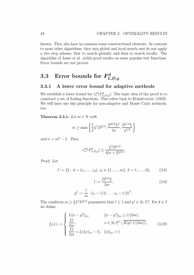
Proof. Let
I := i : i = (i1, . . . , id), ik ∈ 1, . . . , m, k = 1, . . . , d, (3.8)
l :=D2/dL
2m, (3.9)
yi :=l
m· (i1 − 1/2, . . . , id − 1/2)T .
The condition m ≥ 12L2D2/d guarantees that l ≤ 1 and yi ∈ [0, 1]d. For i ∈ I
we define
fi(x) :=
L‖x− yi‖∞, ‖x− yi‖∞ ≤ l/(2m),
Ll
2m, x ∈ [0, l]d \B(yi , l/(2m)),
Ll
2m+ L(‖x‖∞ − l), ‖x‖∞ > l.
(3.10)

3.3. ERROR BOUNDS FOR F dL,D,% 45
0
0.2
0.6
0 0.2 0.4 0.6 0.8 1
0.4
Figure 3.1: fi for d = 1, L = 2, D = 1, m = 5, i = 4.
We show fi ∈ F dL,D,%. Obviously, fi is Lipschitz with constant L. For the
level sets we have
λd(A(fi , 0)) = 0, λd(A(fi , Ll/(2m))) = ld = D(Ll/(2m))d/2.
Since m ≥ D2/dL2/(4%) we know that % ≥ Ll/(2m) and consequently, thatλd(A(fi , %)) ≤ (l + %/L− l/(2m))d. So,
if l + %/L− l/(2m) ≤ D1/d%1/2 then λd(A(fi , %)) ≤ D%d/2.
Since %1/2 < 12D1/dL and since l − l/(2m) ≤ 1
2D1/d%1/2 is guaranteed by
m ≥ D1/dL/%1/2 we conclude λd(A(fi , %)) ≤ D%d/2. Application of Lemma1.2.1 delivers fi ∈ F d
L,D,%.
Let An = φ N be an algorithm that uses at most n function calls. Thenthere exist (at least) two different i , j ∈ I such that
N(fi ) = N(fj ).
No matter where the algorithm chooses x∗ = φ N(fi) = φ N(fj ), wewill have fi(x∗) ≥ Ll/(2m) or f j (x∗) ≥ Ll/(2m), but min fi = min fj = 0.Consequently,
∆(An, FdL,D,%) ≥
l L
2m=
L2D2/d
4(n+ 2)2/d.
Since An was arbitrary we have the same bound for eadn (F dL,D,%).
3.3.2 Optimality and universality of the algorithms ofChapter 2
Corollary 3.3.2. The algorithms (S(L, k))k∈N and (Z(h, k))k∈N have theoptimal rate of convergence. In particular, (Z(h, k))k∈N is universal for F
d.

46 CHAPTER 3. OPTIMALITY RESULTS
Proof. We define m0 := dL2D2/d(LD2/d − %)−1e and n(m) := md − 2. Let
n ≥ maxn(m0), 3, ((9/8)d/2 − 1)−1.
We choose m such that n(m− 1) + 1 ≤ n ≤ n(m). Then
en(F dL,D,%) ≥ en(m)(F
dL,D,%) ≥
D2/dL2
4m2≥ D2/dL2
9n2/d.
For k ∈ N, letnk := bDLd/22−d/23(k+1)d/2+1c.
From Theorem 2.1.2 we know that S(L, k) uses at most nk oracle calls anddelivers an error level
∆(S(L, k), F dL,D,%) ≤ εL,k ≤ D2/dL22−232+2/dn
−2/dk .
This means that the algorithms (S(L, k))k∈N have the optimal rate of con-vergence.
Let m ∈ N. For k ≥ h(m−1)+1 we have ∆(Z(h, k), F dL(m),D,%) ≤ εL(m),h,k
and
cost(Z(h, k), F dL(m),D,%)
≤ α(L(m), d, h, %) + β(L(m), d, h) ε−d/hL(m),h,k + γ(L(m), D, h, d) ε
−2/dL(m),h,k,
with constants α, β, γ that can be determined with Theorem 2.2.2. Recallh ≥ 3. For εL(m),h,k ≤ 1 we have
cost(Z(h, k), F dL(m),D,%) ≤ (α+ β + γ) ε
−2/dL(m),h,k.
Proceeding as for S(L, k)k∈N we see that (Z(h, k))k∈N have the optimal rateof convergence. This means in particular that (Z(h, k))k∈N are universalfor F
d.
3.3.3 A lower error bound for non-adaptive methods
We turn to non-adaptive methods.
Lemma 3.3.3. Let m ≥ max( 14D2/dL)−1, (2D1/d%1/2 − 4%/L)−1, L/(4%).
For n = md − 1 we have
enonn (F d
L,D,%) ≥L
4(n+ 1)1/d.
3.3. ERROR BOUNDS FOR F dL,D,% 47
0
0.4
0.8
1.2
0 0.2 0.4 0.6 0.8 10
0.4
0.8
1.2
0 0.2 0.4 0.6 0.8 1
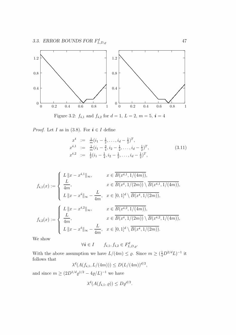
Figure 3.2: fi ,1 and fi ,2 for d = 1, L = 2, m = 5, i = 4
Proof. Let I as in (3.8). For i ∈ I define
xi := 1m
(i1 − 12, . . . , id − 1
2)T ,
xi ,1 := 1m
(i1 − 34, i2 − 1
2, . . . , id − 1
2)T , (3.11)
xi ,2 := 12(i1 − 1
4, i2 − 1
2, . . . , id − 1
2)T ,
fi ,1(x) :=
L ‖x− xi ,1‖∞, x ∈ B(xi ,1, 1/(4m)),
L
4m, x ∈ B(xi , 1/(2m)) \B(xi ,1, 1/(4m)),
L ‖x− xi‖∞ − L
4m, x ∈ [0, 1]d \B(xi , 1/(2m)),
fi ,2(x) :=
L ‖x− xi ,2‖∞, x ∈ B(xi ,2, 1/(4m)),
L
4m, x ∈ B(xi , 1/(2m)) \B(xi ,2, 1/(4m)),
L ‖x− xi‖∞ − L
4m, x ∈ [0, 1]d \B(xi , 1/(2m)).
We show∀i ∈ I fi ,1, fi ,2 ∈ F d
L,D,%.
With the above assumption we have L/(4m) ≤ %. Since m ≥ ( 14D2/dL)−1 it
follows thatλd(A(fi ,1, L/(4m))) ≤ D(L/(4m))d/2,
and since m ≥ (2D1/d%1/2 − 4%/L)−1 we have
λd(A(fi ,1, %)) ≤ D%d/2.

48 CHAPTER 3. OPTIMALITY RESULTS
Application of Proposition 1.2.1 on the piece-wise linear function g withnodes δ = 0, L/(4m), % and values g(δ) = (δd(A(fi ,1, δ))
1/d yields
∀ 0 ≤ δ ≤ % λd(A(fi ,1, δ)) ≤ D δd/2.
Consequently,fi ,1 ∈ F d
L,D,%.
Analogously, we showfi ,2 ∈ F d
L,D,%.
For an arbitrary method An using n oracle calls, we have that in (at least)one cube
Qi := x ∈ D : (i − (1/m, . . . , 1/m) < x < i/m, i ∈ I,
there is no evaluation. For such an index i , we have
N(fi ,1) = N(fi ,2).
Consequently,
∆(An, FdL,D,%) ≥
L
4m=
L
4(n + 1)1/d.
Since An was arbitrary we have the same bound for enonn (F d
L,D,%).
3.3.4 A lower error bound for randomized methods
Finally, we turn to Monte Carlo methods (MCM). See Section 3.2 for thedefinition of a MCM, its error, and the error numbers σad
n (F ).We obtain a lower bound for σad
n (F dL,D,%) with a method similar to that
in Novak (1988), Section 2.1.9. The following lemma uses the mean errornumbers eadn (P ) for a suitable probability measure P to prove a lower boundfor σad
n (F ):
Lemma 3.3.4. Let P be a Borel measure on F of the sort P =∑m
i=1 ciδfi
with ci ≥ 0 and∑m
i=1 ci = 1. Furthermore, let fi ∈ F for i = 1, . . . , m. Thenwe have
eadn (P ) ≤ σadn (F ).
Proof. See Novak (1988), Proposition 2.1.9.
Lemma 3.3.5. Let m be as in Theorem 3.3.1, even, and n = md/2. Then
σadn (F d
L,D,%) ≥n− 1
n
L2D2/d
8(2n)2/d.
3.3. ERROR BOUNDS FOR F dL,D,% 49
Proof. Let l as in (3.9), and I and fi as in (3.8) and (3.10). Define
g(x) :=
Ll
2m, ‖x‖∞ ≤ l,
Ll
2m+ L max
1≤j≤d(xj − l), ‖x‖∞ > l.
Let FI := fi , i ∈ I. We know from Theorem 3.3.1 that FI ⊂ F dL,D,%. Let
A = φ N be an (adaptive) deterministic algorithm using at most n oraclecalls. For at least n different i ∈ I we have N(fi ) = N(g). Consequently,
∑
f∈FI
(inf f − f(A(f))) ≥ (n− 1)Ll
2m=
(n− 1)L2D2/d
4m2.
The proof is complete with Lemma 3.3.4 using the uniform distribution onFI .
3.3.5 Conclusion
We obtained several results in this chapter:
• Adaptive algorithms: We know from Theorem 3.3.1 that for n largeenough, n ≥ n(L,D, %, d),
eadn (F dL,D,%) ≥
L2D2/d
4(n+ 2)2/d.
Furthermore, we conclude from Theorem 2.1.2 (c) that
eadnk(F d
L,D,%) ≤ 2−232+2/dL2D2/dn−2/d,
for k ≥ maxj(L, %), j(L,D, %, d) and nk := bDLd/22−d/23(k+1)d/2+1c.So,
eadn (F dL,D,%)
L2D2/d
n2/d. (3.12)
• Non-adaptive algorithms: From Lemma 3.3.3 we know that for n largeenough, n ≥ n(L,D, %, d),
enonn (F d
L,D,%) ≥ L (4n+ 1)−1/d.

50 CHAPTER 3. OPTIMALITY RESULTS
On the other hand, F dL,D,% ⊂ F d
L with F dL as defined in Section 3.2.
With Novak (1988), Proposition 1.3.6, we have
enonn (F d
L,D,%) ≤ enonn (F d
L) = O(Ln−1/d)
and conclude that
enonn (F d
L,D,%) L
n1/d. (3.13)
• Randomized algorithms: From Lemma 3.3.5 we know that for n largeenough, n ≥ n(L,D, %, d),
σad(F dL,D,%) ≥
n− 1
n
L2D/d
8(2n)2/d.
On the other hand, we have
σadn (F d
L,D,%) ≤ eadn (F dL,D,%)
since any deterministic algorithm can be seen as a MCM with Diracmeasure. So,
σadn (F d
L,D,%) L2D2/d
n2/d. (3.14)
Since non-adaptive MCM can never be better than adaptive ones weneglected to estimate the error numbers σnon
n (F dL,D,%).
So, for our problem class F dL,D,% adaptiveness is essential for optimal algo-
rithms and yields a quadratic speed-up while randomization cannot yieldany further essential advantage.
Our second method is universal for Fd. Our first method has the optimal
rate of convergence in case that the Lipschitz constant is known.
Chapter 4
Numerical experiments
We will now dicuss some questions that have no theoretical consequence butthat are of practical interest.
• We give advice for a good choice of h. This parameter of the universalalgorithm defines the steepness of the diagonal scheme and influencesthe ratio between global and local search.
• The definitions of the algorithms S(L, · ) and Z( · ) are not precise inone aspect. Consider once more step(L, j) for j ≥ 2, as defined inFigure 2.1. Here, the question is left open in which order the algorithmconsiders the elements of NL,j−1, and those of Y (j). This question wasunimportant for proving error bounds. However, a deliberately chosenorder may yield better results in the nonasymptotic behavior.
• We again refer to the design of step(L, j), j ≥ 2. The question whetheran element of NL,j−1 and its neighboring mesh points (x+ y, f(x+ y)),y ∈ Y (j), will also belong to NL,j depends on the particular order inwhich the points in NL,j−1 are considered. This is a consequence ofthe fact that f∗ may vary during step(L, j). We introduce a version ofZ(h, k) such that the cost and error bounds of Chapter 2 still hold, butthe set NL,j is independent of the order in which the points of NL,j−1
are considered.
These considerations led us to develop different versions of the algorithmZ(h, k). We will introduce them in the next section. We then apply themto a set of test functions presented in Section 4.2. The results are given inSection 4.3. We use them to recommend a particular version. For illustration,we plot the points chosen by this version for three of the test functions.
51

52 CHAPTER 4. NUMERICAL EXPERIMENTS
4.1 Algorithm versions
We want to apply different values of h. We test
h = 2, 3, 4, 5, 8, 12. (4.1)
Note that h = 2 is not covered by the results of Theorem 2.2.2. Furthermore,we introduce three different design features the algorithm may or may nothave and that all concern only the design of step(L, j):
• We say that the algorithm has the feature F1 if it performs step(L, j)in two sub-steps as follows: Divide the set Y (j) into the 2 disjointsubsets
Y (j, 1) :=
d⋃
i=1
e(i),−e(i), Y (j, 2) := Y (j) \ Y (j, 1).
Replace step(L, j) by step(L, j1) and step(L, j2). Step(L,j1) is thesame as step(L, j) with the difference that it uses Y (j, 1) instead ofY (j). Analogously, we define step(L, j2).This way, the new points evaluated in step(L, j) are scattered well notonly after the end of step(L, j), i.e., after approximately |NL,j−1| · 3d
points, but also after approximately |NL,j−1| · 2d points.
• We say the algorithm has the feature F2 if it sorts the elements ofNL,j−1 as follows: Let q ∈ N be a fixed number. Without loss ofgenerality assume q ≤ |NL,j−1| =: p. We write the elements of NL,j−1
in a listNL,j−1 := [ (x1, f(x1)), . . . , (xp, f(xp)) ]
such that
f(xi) ≤ f(xi+1), 1 ≤ i ≤ q − 1, f(xq) ≤ f(xj), q < j ≤ p.
The algorithm shall examine the elements of NL,j−1 in such an order.This way, we examine first those q points that, because of their functionvalue, seem to be most promising. We only sort the first q best pointsinstead of sorting them all, in order not to get an additional logarithmicfactor for the computational cost. We choose q := 2 · d.
• Recall the test (∗) of step(L, j), j ≥ 2. We say the algorithm has the
feature F3 if it uses an additional variable f∗. This variable assumesthe value of f∗ at the very beginning of step(L, j) and will not be
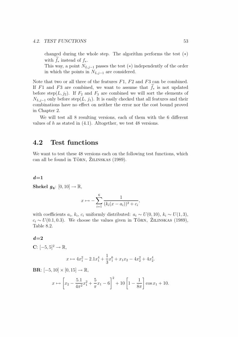
4.2. TEST FUNCTIONS 53
changed during the whole step. The algorithm performs the test (∗)with f∗ instead of f∗.This way, a point NL,j−1 passes the test (∗) independently of the orderin which the points in NL,j−1 are considered.
Note that two or all three of the features F1, F2 and F3 can be combined.If F1 and F3 are combined, we want to assume that f∗ is not updatedbefore step(L, j2). If F2 and F3 are combined we will sort the elements ofNL,j−1 only before step(L, j1). It is easily checked that all features and theircombinations have no effect on neither the error nor the cost bound provedin Chapter 2.
We will test all 8 resulting versions, each of them with the 6 differentvalues of h as stated in (4.1). Altogether, we test 48 versions.
4.2 Test functions
We want to test these 48 versions each on the following test functions, whichcan all be found in Torn, Zilinskas (1989).
d=1
Shekel g6: [0, 10] → R,
x 7→ −6∑
i=1
1
(ki(x− ai))2 + ci,
with coefficients ai, ki, ci uniformly distributed: ai ∼ U(0, 10), ki ∼ U(1, 3),ci ∼ U(0.1, 0.3). We choose the values given in Torn, Zilinskas (1989),Table 8.2.
d=2
C: [−5, 5]2 → R,
x 7→ 4x21 − 2.1x4
1 +1
3x6
1 + x1x2 − 4x22 + 4x4
2.
BR: [−5, 10] × [0, 15] → R,
x 7→[x2 −
5.1
4π2x2
1 +5
πx1 − 6
]2
+ 10
[1 − 1
8π
]cos x1 + 10.

54 CHAPTER 4. NUMERICAL EXPERIMENTS
GP: [−2, 2]2 → R,
x 7→[1 + (x1 + x2 + 1)2(19 − 14x1 + 3x2
1 − 14x2 + 6x1x2 + 3x22)]·[
30 + (2x1 − 3x2)2(18 − 32x1 + 12x2
1 + 48x2 − 36x1x2 + 27x22)].
G2: [−100, 100/√
2]2 → R,
x 7→ 1
200(x2
1 + x22) − cos(x1) · cos(x27
√2) + 1.
The domain given for G2 in Torn, Zilinskas (1989) is [−100, 100]2. Wechanged it because otherwise, the first point evaluated by our algorithmwould already be the global minimizer.
R: [−1, 1/√
2]2 → R,
x 7→ x21 + x2
2 − cos(18x1) − cos(18x2).
We changed the domain [−1, 1]2 given in Torn, Zilinskas (1989) for thesame reason.
d=3
H3: [0, 1]3 → R,
x 7→ −4∑
i=1
ci exp
[−
3∑
j=1
αi,j(xj − pi,j)2
],
with coefficients αi,j and pi,j that can be found in Torn, Zilinskas (1989),p. 185.
d=4
S5, S7, S10: [0, 10]4 → R,
x 7→ −m∑
i=1
1
(x− A(i))(x− A(i))T + ci.
with vectors A(i) and coefficients ci that can again be found in Torn,Zilinskas (1989), p. 184.
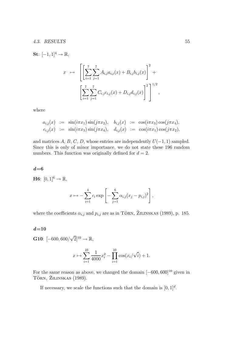
4.3. RESULTS 55
St: [−1, 1]4 → R,
x 7→
[
7∑
i=1
7∑
j=1
Ai,jai,j(x) +Bi,jbi,j(x)
]2
+
[7∑
i=1
7∑
j=1
Ci,jci,j(x) +Di,jdi,j(x)
]2
1/2
,
where
ai,j(x) := sin(iπx1) sin(jπx2), bi,j(x) := cos(iπx3) cos(jπx4),
ci,j(x) := sin(iπx3) sin(jπx4), di,j(x) := cos(iπx1) cos(jπx2),
and matrices A, B, C, D, whose entries are independently U(−1, 1) sampled.Since this is only of minor importance, we do not state these 196 randomnumbers. This function was originally defined for d = 2.
d=6
H6: [0, 1]6 → R,
x 7→ −4∑
i=1
ci exp
[−
6∑
j=1
αi,j(xj − pi,j)2
],
where the coefficients αi,j and pi,j are as in Torn, Zilinskas (1989), p. 185.
d=10
G10: [−600, 600/√
2]10 → R,
x 7→10∑
i=1
1
4000x2
i −10∏
i=1
cos(xi/√i) + 1.
For the same reason as above, we changed the domain [−600, 600]10 given inTorn, Zilinskas (1989).
If necessary, we scale the functions such that the domain is [0, 1]d.

56 CHAPTER 4. NUMERICAL EXPERIMENTS
h 2 3 4 5 8 12
Feature
no feature 670 666 697 684 749 841
F1 701 640 784 767 849 977
F2 423 266 283 293 313 394
F3 663 742 744 667 740 784
F1, F2 609 572 568 620 698 807
F1, F3 658 553 631 743 674 748
F2, F3 495 407 442 475 483 470
F1, F2, F3 512 513 452 516 508 552
Table 4.1: Results for the summed up rank numbers
4.3 Results
For each function, we compare the values of f∗ after 250, 1,500 and 10,000oracle calls and rank the 48 versions. This results in 39 different rankings.For each algorithm version we sum up all its rank numbers. We state theresults in Table 4.1.
The results make it easy to give advice: The version with h = 3 and F2has the least value. Furthermore, the result for F2 is best for any value ofh. Also, the column for h = 3 has 5 times the best and 2 times the secondbest value.
We suggest to use Z(3, · ) with Feature F2.
We give the results for this version in Table 4.2 and plots of the points itchooses for the functions Shekel g6, C, and BR.

4.3. RESULTS 57
d fct. n = 250 n = 1, 500 n = 10, 000 glob. min.
1 g6 -10.05863092 -10.05869313 -10.05869313
2 C -0.990514469 -1.031480295 -1.031625022 -1.0316285
BR 0.397935486 0.397887448 0.397887387 ≈ 0.398
GP 3.064984070 3.000811378 3.000010033 3
G2 0.0088591487 0.0006864435 0.0000009992 0
R -1.031206852 -1.871066950 -1.999970549 -2
3 H3 -3.862583278 -3.862698023 -3.862724551 -3.86
4 S5 -1.631190022 -10.15319696 -10.15319696 ≈ -10
S7 -1.945297979 -10.40282047 -10.40293718 ≈ -10
S10 -7.216953325 -10.53629007 -10.53640678 ≈ -10
6 H6 -2.035737075 -3.168159945 -3.203076797 -3.32
10 G10 20.30238203 20.30238203 20.30238203 0
Table 4.2: The results for the version with h = 3 and feature F2. The righthand side column gives the minimum value according to Torn, Zilinskas(1989). The minimum of g6 given there is -13.9223449 and seems to be wrong.It should be attained at x0 := 4.8555654, but g6(x0) = −8.937. For St, theminimum depends on the random numbers. In consequence, we have no valuewhich we could compare to ours. ForG10 the approximation of our algorithmis not too good even after 10,000 points. This is not surprising since here,d = 10. The first improvement is after n = 59114 points: f∗ = 9.730. Aftern = 67789 points we have f∗ = 2.662.

58 CHAPTER 4. NUMERICAL EXPERIMENTS
Plots for Shekel g6
-10
-8
-6
-4
-2
0
0 2 4 6 8 10
-10
-8
-6
-4
-2
0
0 2 4 6 8 10
-10
-8
-6
-4
-2
0
0 2 4 6 8 10
-10
-8
-6
-4
0
0 4 6 8 10
-2
2
Figure 4.1: The points chosen by Z(3, 8), Z(3, 12), Z(3, 14), Z(3, 16) for g6.
function algorithm # points f∗Shekel g6 Z(3, 8) 27 -8.383952678
Z(3, 12) 60 -9.575211370Z(3, 14) 115 -9.871841283Z(3, 16) 162 -10.05469879
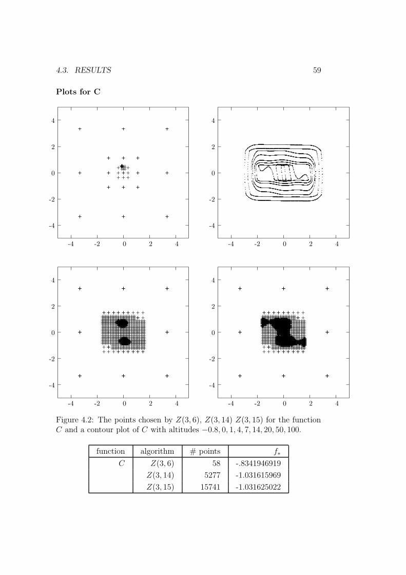
4.3. RESULTS 59
Plots for C
-4
-2
0
2
4
-4 -2 0 2 4
-4
-2
0
2
-4 -2 0 2 4
4
-4
-2
0
2
4
-4 -2 0 2 4
-4
-2
0
2
4
-4 -2 2 40
Figure 4.2: The points chosen by Z(3, 6), Z(3, 14) Z(3, 15) for the functionC and a contour plot of C with altitudes −0.8, 0, 1, 4, 7, 14, 20, 50, 100.
function algorithm # points f∗
C Z(3, 6) 58 -.8341946919
Z(3, 14) 5277 -1.031615969
Z(3, 15) 15741 -1.031625022

60 CHAPTER 4. NUMERICAL EXPERIMENTS
Plots for BR
0
2
4
6
8
10
12
14
-4 -2 0 2 4 6 8 10
0
2
4
6
8
10
12
14
-4 -2 0 2 4 6 8 10
0
2
4
6
8
10
12
14
-4 -2 0 2 4 6 8 10
0
2
4
6
8
10
12
14
-4 -2 0 2 4 6 8 10
Figure 4.3: The points chosen by Z(3, 5), Z(3, 10), Z(3, 11) for BR, and acontour plot of BR with altitudes 1, 4, 7, 11, 19, 27, 50, 100.
function algorithm # points f∗
BR Z(3, 5) 42 0.434202095
Z(3, 10) 3988 0.397887448
Z(3, 11) 11788 0.3978878368
Chapter 5
Applications
We present two applications of the fine-tuned version of our universal algo-rithm.
5.1 Banach-Mazur distance
Let E, F,G be n-dimensional normed vector spaces. The Banach-Mazurdistance of E and F is defined by
d(E, F ) := inf‖T‖ · ‖T−1‖, T : E → F linear isomorphism. (5.1)
It measures how far the unit ball of E is from an affine image of the unit ballof F . It also shows how much numerical parameters of E can differ from thecorresponding ones of F . We have
d(E,G) ≤ d(E, F ) · d(F,G).
Furthermore, log d(·, ·) is a semi-metric on the set of all n-dimensional normedvector spaces with log d(E, F ) = 0 if E and F are isometric. We say Fbelongs to the class [E] if log d(E, F ) = 0.
Let Mn be the set of all classes of n-dimensional normed vector spaces.Mn is compact for all n ∈ N and is called the Minkowski compactum, seeTomczak-Jaegermann (1989), Chapter 9, for this and also to learn moreabout the Banach-Mazur distance. For
diam Mn := sup[E],[F ]∈Mn
d(E, F )
we know that for an unknown constant c independent of the dimension n
c · n ≤ diam Mn ≤ n.
61
62 CHAPTER 5. APPLICATIONS
The first inequality is due to John (1948), the second one is a corollary ofGluskin (1981). For dimensions n > 2 the exact value of diam Mn is notknown.
In our application we consider the case n = 3 and the particular spacesl31 and l3∞ being R
3 endowed with the norms
‖ x | l31 ‖ :=
3∑
i=1
|xi| and ‖ x | l3∞ ‖ := max1≤i≤3
|xi|,
respectively. For the linear isomorphism
T : l31 → l3∞, x 7→
1 −1/3 11 1 −1/3
−1/3 1 1
x,
we know ‖T‖ · ‖T−1‖ = 95. The conjecture is that this value is already best
possible, i.e., that d(l31, l3∞) = 9
5. This would imply
diam M3 ≥9
5.
We want to test this hypothesis by applying our universal algorithm. Asa first step, we reformulate the problem:
“Minimize ‖T‖ · ‖T−1‖ for T : l31 → l3∞ linear isomorphism” (5.2)
to an optimization problem with a 6-variate objective defined on the domain[−1, 1]6.
For the rest of this section, T will denote a linear isomorphism from l31to l3∞. Without loss of generality, we assume
‖T‖ = 1.
Let (ti,j)3i,j=1 be the matrix associated to T in the usual way. In our special
situation T : l31 → l3∞, we know ‖T ‖ = maxi,j=1,...,3 |ti,j|. A simple argumentshows that we can restrict our search to isomorphisms that can be identifiedwith a matrix as follows:
T ∼
1 t1,2 t1,3
t2,1 1 t2,3
t3,1 t3,2 1
, ti,j ∈ [−1, 1]. (5.3)
Let e(1), e(2), e(3) be the unit vectors in R3. Then
T ∼(Te(1)
∣∣Te(2)∣∣Te(3)
)=:(y(1)∣∣y(2)
∣∣y(3)).

5.1. BANACH-MAZUR DISTANCE 63
For x ∈ R3 we define λT
1 (x), λT2 (x), λT
3 (x) to be the (unique) solutions of
3∑
i=1
λTi (x)y(i) = x ⇔
3∑
i=1
λTi (x)e(i) = T−1x.
We conclude that
‖T−1x | l31 ‖ =3∑
i=1
|λTi (x)|.
One verifies easily that
‖T−1‖ = supx6=0
‖T−1x | l31 ‖‖ x | l3∞‖ = max
1≤j≤4
3∑
i=1
|λTi (v(j))|,
with
v(1) :=
111
, v(2) :=
11−1
, v(3) :=
1−11
, v(4) :=
−111
. (5.4)
Then,
d(l31, l3∞) = inf
‖T ‖=1max1≤j≤4
3∑
i=1
|λTi (v(j))|.
The coefficients λTi (x) can be calculated by
λT1 (x) =
det(x | y(2) | y(3)
)
det (y(1) | y(2) | y(3)), λT
2 (x) =det(y(1) | x | y(3)
)
det (y(1) | y(2) | y(3)),
λT3 (x) =
det(y(1) | y(2) | x
)
det (y(1) | y(2) | y(3)).
Since every T we want to consider can be identified with one point in [−1, 1]6,as done in (5.3), we reformulate (5.2) to:
“Minimize the objective
x 7→ max1≤j≤4
detT1(x, v(j)) + detT2(x, v
(j)) + detT3(x, v(j))
detT (x), x ∈ [−1, 1]6 \Ω0,
with
T1(x, v(j)) :=
v(j)1 x3 x5
v(j)2 1 x6
v(j)3 x4 1
, T2(x, v
(j)) :=
1 v(j)1 x5
x1 v(j)2 x6
x2 v(j)3 1
,
T3(x, v(j)) :=
1 x3 v(j)1
x1 1 v(j)2
x2 x4 v(j)3
, T (x) :=
1 x3 x5
x1 1 x6
x2 x4 1
,

64 CHAPTER 5. APPLICATIONS
# points f∗ x∗
250 2.3846154(0, 0, 0, 2
3, 0, −2
3
)
1500 2.1172414(0, 0, 0, 8
9, 0, −9
9
)
10,000 1.8077816(
242243, −82
242, −82
243, 242
243, 242
243, −80
243
)
100,000 1.8025930(
728729, 242
729, −244
729, −728
729, −728
729, 244
729
)
1,000,000 1.8008642(
21862187
, 7282187
, −7302187
, −21862187
, −21862187
, 7302187
)
2,000,000 1.8000960(
1968219683
, 656019683
, −656219683
, −1968219683
, −1968219683
, 656219693
)
Table 5.1: Results
v(j) as in (5.4), and Ω0 := x ∈ [−1, 1]6 : detT (x) = 0.”Applying our algorithm, we ignored the existence of Ω0. This is possiblebecause all singularities are on the border of the domain while all evaluationpoints are in its interior. The results are stated in Table 5.1.
Our results confirm the conjecture diam M3 ≥ 95.
5.2 Mean errors in global optimization
We consider a function space F endowed with a probability measure P de-fined on a suitable σ-algebra. We present a scheme of how the universalalgorithm, or a suitable modification, can be used to prove an upper boundfor the mean error numbers eadn (P ) as defined in (3.4). We try to apply thisscheme to the particular case F = C[0, 1] and P the Wiener measure P ∗.
5.2.1 Basic scheme
Let (Ωi) be a sequence of subsets of F such that
Ω0 := ∅,
Ωi ⊂ Ωi+1,
P (⋃
i∈N
Ωi) = 1.
5.2. MEAN ERRORS IN GLOBAL OPTIMIZATION 65
Furthermore, for a sequence pi ↓ 0 with p0 := 1
P (Ωi) ≥ 1 − pi
shall be fulfilled. Let (Yn)n∈N be a sequence of optimization algorithms withYn using at most n function values. Concerning the sets Ωi, their worst-caseerror shall be estimated by a sequence (εn,i)n,i∈N:
∆(Yn,Ωi) ≤ εn,i. (5.5)
Without loss of generality, we assume the sequence (εn,i)n∈N to be monotonedecreasing for fixed i. We need the following technical result.
Proposition 5.2.1. Let I ∈ N. Then
I∑
i=1
εn,iP (Ωi \ Ωi−1) ≤I∑
i=1
εn,i(pi−1 − pi) + εn,I[P (ΩI) − (1 − pI)].
Proof. Recall Ω0 = ∅ and p0 = 1. For I = 1 we have
εn,1P (Ω1 \ Ω0) = εn,1(1 − p1) + εn,1(p1 − 1 + P (Ω1 \ Ω0))
= εn,1(p0 − p1) + εn,1[P (Ω1) − (1 − p1)].
For I + 1 we have by induction
I+1∑
i=1
εn,iP (Ωi \ Ωi−1) ≤I∑
i=1
εn,i(pi−1 − pi) + εn,I[P (ΩI) − (1 − pI)] +
εn,I+1P (ΩI+1 \ ΩI)
=
I+1∑
i=1
εn,i(pi−1 − pi) + εn,I+1[P (ΩI+1) − (1 − pI+1)]
+ (εI+1 − εI︸ ︷︷ ︸≥0
)[(1 − pI) − P (ΩI)︸ ︷︷ ︸≤0
]
≤I+1∑
i=1
εn,i(pi−1 − pi) + εn,I+1[P (ΩI+1) − (1 − pI+1)].
Lemma 5.2.2. Assume that the error ∆(Y1, P ) is finite and that
limI→∞
ε1,I [P (ΩI) − (1 − pI)] = 0. (5.6)
Then the average error is bounded by
∆(Yn, P ) ≤∞∑
i=1
εn,i (pi−1 − pi). (5.7)
66 CHAPTER 5. APPLICATIONS
Proof. For I ∈ N we have
∆(Yn, P ) =
∫
C[0,1]
|f(Yn(f)) − inf f | dP (f)
≤I∑
i=1
εn,iP (Ωi \ Ωi−1) +
∫
C[0,1]\ΩI
|f(Yn(f)) − inf f | dP (f).
Application of Proposition 5.2.1 yields
∆(Yn, P ) ≤I∑
i=1
εn,i(pi−1 − pi) + εn,I[P (ΩI) − (1 − pI)] +
∫
C[0,1]\ΩI
|f(Yn(f)) − inf f | dP (f).
Taking the limit I → ∞ we get
∆(Yn, P ) ≤∞∑
i=1
εn,i(pi−1 − pi).
Remark 5.2.3. For the Wiener measure P ∗ on C[0, 1] it is known thatE(inf f) = −
√2/π, so ∆(Yn, P
∗) is finite for any method Y1 that returns apoint x∗ ∈ 0, x(1).
5.2.2 The Wiener measure
For a definition of the Wiener measure P ∗ we refer to Partzsch (1984) orRevuz, Yor (1990).
For the mean error in global optimization the following results are known.Ritter (1990) shows that a best non-adaptive method has an error ofO(n−1/2) where n is the number of used function calls. As a consequence,there exists a constant C1 such that
eadn (P ∗) ≤ C1 · n−1/2.
Calvin (2004) shows that the mean error cannot decrease exponentially:
∀C2, C3 > 0 ∃n ∈ N eadn (P ∗) > C2 · exp(−C3 · n).
There is a huge gap between the lower and the upper bound. We try to applythe concept of the previous section to improve the upper bound. Let
α ∈ (0, 1/2) (5.8)

5.2. MEAN ERRORS IN GLOBAL OPTIMIZATION 67
and L(i) as in (2.8). For the sets
Ω′i := f ∈ C[0, 1] : ∀x, y ∈ [0, 1] |f(x) − f(y)| ≤ L(i) |x− y|α
Novak et al. (1995), Lemma 3.1, show as a corollary to Ledoux, Tala-grand (1991), Lemma 3.1, that
∀i ∈ N P ∗(Ω′i) ≥ 1 − c1 exp(−c2L(i)2)
for some constants c1, c2 > 0. Note that we have Holder- instead of Lip-schitz continuity. We will adopt Z(h, k) to this new situation. ReconsiderFigure 2.1. By changing the test (∗) to
f(x) ≤ f∗ + L[2−13−j+2
]α
we obtain a version of Z(h, k) that we call
Z(h, α, k).
This one can be applied to the new situation. It is easy to check that
∆(Z(h, α, k),Ω′i) ≤ L(i)
[2−13−k+h(m−1)+1
]α.
From Novak (1988) we know that eadn (Ω′i) = enon
n (Ω′i) = L(i)(2n)−α. As a
consequence, for εn,i as in (5.5) we have
εn,i = O(n−α).
Since α < 1/2 it is impossible to obtain an estimate as in (5.7) that is betterthan the result obtained by Ritter.
It would be helpful in this situation to have an additional estimate ofthe following kind: Let g : [0,∞) → [0, 1] with g(0) = 0 be increasing andh : [0,∞) → [0, 1] be decreasing such that
P ∗
(⋂
δ>0
f ; λ(A(f, δ)) ≤ Dg(δ))
≥ 1 − h(D). (5.9)
Then, with a suitable sequence (D(i))i∈N another sequence of sets (Ω′′i )i∈N
could be constructed:
Ω′′i := f ∈ C[0, 1] : ∀δ > 0 λ(A(f, δ)) ≤ D(i) g(δ).
We defineΩi := Ω′
i ∩ Ω′′i
68 CHAPTER 5. APPLICATIONS
and obtain
P ∗(Ωi) ≥ 1 − c1 exp(−c2L(i)2) − h(D(i)).
If Condition (5.6) is fulfilled we can apply our basic scheme. Then, a costestimation as that of Theorem 2.2.2 could be established. However, it seemsthat a result as in (5.9) is not known.
We refrain from theoretical speculations. Instead, we are interested inhow the algorithms Z(h, α, · ) behave in a numerical experiment.
5.2.3 Numerical simulation
We use the algorithms Z(h, α, · ) to determine numerically an upper boundfor the error numbers eadn (P ∗). We found the diploma thesis of Nestel (1988)very useful for this purpose. In Chapter 4, he treats problems occurring whenthe rate of convergence of mean errors is to be determined if the Wienermeasure is assumed. We only sketch how we proceed and refer to Nestel(1988) for details.
As a first step, we introduce the algorithms
Yn, n ∈ N,
which are basically the same methods as (Z(h, α, k))k∈N with h = 3, FeatureF2 and α = 0.49. The difference is that Z(h, α, k) stops after k diagonalswhile Yn is defined to stop after n function calls. Furthermore, Yn uses theinformation P ∗(f(0) = 0) = 1.
We want to determine numerically the behavior of
∆(Yn, P∗) =
∫
C[0,1]
[f(Yn(f)) − inf f ]P ∗(df)
for n→ ∞.
Simulation of f(Yn(f))
For simulating f(Yn(f)) we can use the fact that for applying Yn to a pathf we do not need to simulate the whole path but only its function valuesat the points x(1), . . . , x(n) that are used by Yn. The following method is anapplication of the Levy-Cielsielski representation of Brownian motion, seePartzsch (1984), pp. 26, for details. Let
X1, . . . , Xn

5.2. MEAN ERRORS IN GLOBAL OPTIMIZATION 69
be realizations of independent standard normal distributed random variables.The first point x(1) evaluated by Yn is 0.5. We set
f(x(1)) =√
1/2 ·X1.
Now let 2 ≤ i ≤ n. Without loss of generality we assume x(1) ≤ · · · ≤ x(i−1).We define x(0) := 0 and set f(x(0)) := 0. For x(i) we have to consider threecases:
1. x(i) ∈ (x(j−1), x(j)) for some 1 ≤ j ≤ i− 1. We set
f(x(i)) :=f(x(j−1)) · (x(j) − x(i)) + f(x(j)) · (x(i) − x(j−1))
x(j) − x(j−1)+
Xi ·√
(x(i) − x(j−1)) · (x(j) − x(i))
x(j) − x(j−1).
2. x(i) = x(j) for some 1 ≤ j ≤ i− 1. We set
f(x(i)) := f(x(j)).
3. x(i) > x(i−1). We set
f(x(i)) := f(x(i−1)) +Xi ·√x(i) − x(i−1).
Finally, we set
f(Yn(f)) := min1≤i≤n
f(x(i)).
Now we know how to simulate f(Yn(f)) for a path of the Brownian motion.We present two different methods of how to determine ∆(Yn, P
∗) numerically.
Direct simulation
Let Y(1)n , . . . , Y
(l)n be the realizations of l independent copies of the random
variable f(Yn(f)). The direct simulation uses the discretization
∆(Yn, P∗) ≈ 1
l
l∑
i=1
Y (i)n +
√2
π=: ∆(l)(Yn, P
∗). (5.10)

70 CHAPTER 5. APPLICATIONS
Simulation using local errors
Again, let x(1), . . . , x(n) be the points chosen by Yn. The information vectorused by Yn is given by
Nn : C[0, 1] → Rn, f 7→ (f(x(1)), . . . , f(x(n))).
Nn is a random variable. Let P ∗Nn
denote its distribution. We use the desin-tegration
∆(Yn, P∗) =
∫
Rn
∫
C[0,1]
(f(Yn(f)) − inf f)P ∗(df |Nn = y)P ∗Nn
(dy)
=
∫
Rn
[min0, y1, . . . , yn −
∫
C[0,1]
inf fP ∗(df |Nn = y)]
︸ ︷︷ ︸local error ∆(Yn,P ∗,y)
dP ∗Nn
(y).
Let Y(1)n , . . . , Y
(l)n be the realizations of l independent copies of f(Yn(f)) and
N(1)n , . . . , N
(l)n be the according information vectors. The simulation with
local errors uses the discretization
∆(Yn, P∗) ≈ 1
l
l∑
i=1
[Y (i)
n −∫
C[0,1]
inf fP ∗(df |Nn = N (i)n )
]=: ∆(l)(Yn, P
∗).
(5.11)
The simulation ∆(l)(Yn, P∗) is by far more complicated than ∆(l)(Yn, P
∗)
since we have to compute the local errors ∆(Yn, P∗, N
(i)n ) numerically. On
the other hand, ∆(l)(Yn, P∗) has a decisive advantage, as we will see in the
next section.
Asymptotic cost
Both ∆(l)(Yn, P∗) and ∆(l)(Yn, P
∗) are realizations of random variables, say
∆(l)n and ∆
(l)n . Let us consider ∆
(l)n first. In order to obtain a meaningful
result, we require for the standard deviation, its mean value, and a constant0 < c < 1 that
σ(∆(l)n ) ≤ c · E(∆(l)
n ). (5.12)
This has consequences for the choice of l = l(n). Empirical results lead us toassume that
∀n ∈ N σ(f(Yn(f))) ≈ σ(inf f).
Consequently,σ(∆(l)
n ) ≈ n−1/2σ(inf f).

5.2. MEAN ERRORS IN GLOBAL OPTIMIZATION 71
If we want to test the conjecture ∆(Yn, P∗) = O(n−p) for some p > 0 then
we needl(n) = O(n2p)
runs, i.e. O(n2p+1) function calls / random numbers.
Example 5.2.4. Consider the algorithm An that chooses the points equidis-tantly: Nn := (f(1/n), f(2/n), . . . , f(1)). We know from Ritter (1990)that it has a convergence rate of n−1/2. For n = 21 knots we need l = 100runs in order to get
σ(∆(l)(An, P∗)) ≤ 0.5 · E(∆(l)(An, P
∗)).
For n = 18.000, we need l = 90.000 runs, see Nestel (1988) for details.Now let us assume a rate of convergence of 1 instead of 0.5. Then, these90.000 runs are already necessary for n = 134 ≈
√18000. We see that the
direct simulation is problematic in examining asymptotic behavior for “high”convergence rates.
The situation is better for ∆(l)(Yn, P∗) because the standard deviation of
the local error is decreasing with l. Nestel (1988) gives the upper bound
σ2(f(Yn(f))) ≤ L
2,
where L is the length of the longest subinterval that is induced by the pointsx(1), . . . , x(n). The empirical standard deviations decreases much quicker. Letus assume that σ(f(Yn(f))) = O(n−q). To fulfill condition (5.12) we need
l(n) = O(n2(p−q))
runs, i.e., O(n2(p−q)+1) function calls / random numbers. We want to usethis advantage towards direct simulation.
Calculating the local error
We sketch how we calculate the local error numerically, i.e., for y ∈ Rn we
want to approximate
Ey(inf f) :=
∫
C[0,1]
inf f P ∗(df |Nn = y).
We implement the calculation in Maple, using the standard accuracy of tendigits. We proceed in 4 steps.

72 CHAPTER 5. APPLICATIONS
1. Let P ∗y := P ∗( · |Nk = y). For y = (y1, . . . , yk) let y0 := min0, y1, . . . , yk.
With partial integration we get
Ey(inf f) =
∫ y0
−∞
uP ∗y (inf f = u) du = y0 −
∫ y0
−∞
P ∗y (inf f ≤ u) du
= y0 −∫ y0
−∞
[1 − P ∗y (inf f > u)] du.
Assume 0 = x(0) < · · · < x(n) < 1. Then we know (see, e.g., Partzsch(1984), Behauptung 4.3)
P ∗( infx(j−1)≤x≤x(j)
f(x) > u | f(x(j−1)) = yj−1, f(x(j)) = yj)
=
1 − exp(−2
(yj−1−u)(yj−u)
x(j)−x(j−1) ), u < minyj−1, yj,0, else.
For x(n) ≤ x ≤ 1 we have
P ∗( infx(n)≤x≤1
f(x) > u | f(x(n)) = yn) =
2Φ
(yn−u√1−x(n)
)− 1, u < yn,
0, else,
with Φ the distribution function of the standard normal distribution. Fork independent random variables Zj we know
P ( min1≤j≤k
Zj > u) =
k∏
j=1
P (Zj > u).
So,
Ey(inf f) =
∫ y0
−∞
[1 − P ∗y (inf f > u)] du (5.13)
= y0 −∫ y0
−∞
[1 −
[2Φ
(yn−u√1−x(n)
)− 1
] k∏
j=1
(1 − exp(−2(yj−1−u)(yj−u)
x(j)−x(j−1) ))
︸ ︷︷ ︸h(u)
]du.
2. To approximate (5.13), we cannot integrate over (−∞, y0] but only over afinite interval. Let ε be the accuracy we want to determine the integral with.Let L be the length of the longest subinterval induced by the evaluationpoints, let
z0 := y0 −√−L
4ln(0.5πLε2), zi+1 := (zi + y0)/2.
5.2. MEAN ERRORS IN GLOBAL OPTIMIZATION 73
For j such that h(zj+1) > ε and h(zj) ≤ ε, choose [zj, y0] as the integrationinterval. Then, the maximal error is less than ε. We choose ε := 10−1.5·log(n).
3. To approximate h(u) we use logarithmic calculation. Define
qj := exp(−2(yj−1 − u)(yj − u)
x(j) − x(j−1)), pj := 1 − qj.
We usek∏
j=1
pj = exp(∑k
j=1 ln pj).
Because very often qj 1 we can calculate ln pj with the Taylor expansion
ln(1 − q) = −∑∞j=1
qj
j. A faster converging method is ln( 1−u
1+u) = ln(1 − q)
with u = q2−q
. We get the Taylor expansion
ln(1 − u
1 + u) = −2
∞∑
j=0
u2j+1
2j + 1. (5.14)
We take the first 10 summands of (5.14). For the calculation of Φ we use thesubroutine of Maple.
4. To calculate∫ y0
zjh(u) du numerically, we take into consideration that h(u)
decreases quickly for u decreasing. We can exploit that h is smooth. Weuse Romberg integration, see, e.g., Kincaid, Cheney (2002) for details. Toapproximate
I(f) =
∫ b
a
f(x) dx
we introduce
R(0, 0) :=1
2(b− a)[f(a) + f(b)],
R(j, 0) :=1
2R(j − 1, 0) + hj
2j−1∑
i=1
f(a+ (2i− 1)hj
R(j,m) := R(j,m− 1) +1
4m − 1[R(j,m− 1) −R(j − 1, m− 1)], m ≤ j,
with h0 := b−a and hj = hj−1/2 for j ≥ 1. The Romberg integration R(j, j)is an O(h2j
j ) approximation of I(f) if f ∈ C2j [a, b]. We use R(6, 6).

74 CHAPTER 5. APPLICATIONS
n ∆(l)(Yn, P∗) σ(f(Yn(f))) σ(∆(l)(Yn, P
∗))
12 0.07438209115 0.02342877456 0.01171438728
25 0.02201084315 0.02010604556 0.006358089871
50 0.008856878920 0.01525149098 0.003410337058
100 0.003076658378 0.006514667583 0.001030059388
200 0.001130572636 0.004480232594 0.0005009052314
400 0.00003234345839 0.0001537732155 0.00001215684010
800 0.00003342611825 0.0004077644289 0.00002279472453
1600 0.000009293359809 0.0001084567565 0.000004287129726
Table 5.2: Results for the simulated mean error
10−5
10−4
10−3
10−2
10−1
10 100 1000
Figure 5.1: The simulated mean error on a logarithmic scale.
Results
We determined numerically the values of ∆(l)(Yn, P∗) for
n = 12, 25, 50, 100, 200, 400, 800, 1600.
We assumed a rate of convergence of the error of at least n−1 and a rate ofn−1/2 for the standard deviation of the local error. In order to fulfill (5.12)we set l(n) := dc ·ne with c := 0.4. In addition to the result for ∆(l)(Yn, P
∗),

5.2. MEAN ERRORS IN GLOBAL OPTIMIZATION 75
we also recorded the empirical standard deviation of the local error, and theempirical standard deviation of ∆(l)(Yn, P
∗), see Table 5.2 for the results.They show that the number l(n) of iterations was chosen reasonably.
A least-square fit of the logarithmized data suggests to assume a depen-dence of
∆(Yn, P∗) ≈ 13.12 · n−1.93,
which is represented by the dotted line in Figure 5.1.


Notations
A(f, δ) 5 level setA, A(f) 15 optimization algorithmAad
n (F ) 38 class of adaptive methodsAnon
n (F ) 38 class of non-adaptive methods 41B(x, r, ‖ · ‖) 7 ballB(x, r) 8 ballcost(A, f) 15 function-wise errorcost(A, F ) 15 worst-case costc(d, h) 23 constantC(L, d, h) 23 constantd · e 22 ceiling functionD 5 class parameterD 33 domain∆(A, f) 37 function-wise error∆(A, F ) 37 worst-case error∆(A, P ) 41 mean error∆(Q, f) 42 error∆(Q,F ) 42 errorei 15 unit vector in R
d
eadn (F ) 39 error numberenon
n (F ) 39 error numbereadn (P ) 41 mean error numbersenon
n (P ) 41 mean error numbersεL,k 17 error levelεL,h,k 23 error levelF d
L,D,% 5 function classf∗ 17 approximationF 33 problem classF
d 10 class of problem classes F dL,D,%
77

78 NOTATIONS
j(L, %) 17 constantj(L,D, %, d) 17 constantj(m, i, %) 24 constantj ′(m, i, h, %) 25 constantL 5 Lipschitz parameterL(i) 22 Lipschitz parameterlastconst 20 control functionlaststep 20 control functionM 16 midpoint (1/2, . . . , 1/2)mesh(j) 16 equidistant meshMC(Aad
n (F )) 42 set of adaptive MCMsMC(Anon
n (F )) 42 set of non-adaptive MCMsNL,j 17N∗
L,j 18N 36 information vector
12
:= (1, . . . , 1)T
P 41 probability measureP ∗ 41 Wiener measureφ 37 mappingQ 42 Monte Carlo methodRk 34 registerrk 34 real number in register% 5 class parameterS(L, k) 17 non-universal algorithmstep(L, j) 17step(L, 1′) 20σad
n (F ) 42 error numberσnon
n (F ) 43 error numberx∗ 7 global minimizerx∗ 15 approximationY (j) 15 set of scaled vectorsZ(k) 21 universal algorithmZ(h, k) 23 universal algorithm

Bibliography
Babuska, I. (1968), Uber universal optimale Quadraturformeln, in Appl.Mat. 13, pp. 304-338, 338-404.
Bakhvalov, N. S. (1959), On approximate computation of multiple in-tegrals (in Russian), in Vestnik Moscow Univ. Ser. I Mat. Mekh. 4, pp.3-18.
Borgwardt, K.H. (1987), The Simplex Method. A Probabilistic Analysis,Springer, Berlin.
Brass, H. (1988), Universal quadrature rules in the space of periodic func-tions, in Numerical Integration III, eds. H. Brass and G. Hammerlin, ISNM85, pp. 16-24, Birkhauser, Basel.
Calvin, J. M. (2004), Lower bounds on complexity of optimization ofcontinuous functions, in Journal of Complexity, 20, pp. 773-795.
Gluskin, E. D. (1981), The diameter of the Minkowski compactum isapproximately equal to n, in Functional Analysis and its Applications 15(1), pp. 57-58.
Griebel, M., Woznakowski, H. (2005), On the optimal convergencerate of universal and non-universal algorithms for multivariate integrationand approximation, preprint.
John, F. (1948), Extremum problems with inequalities as subsidiary con-ditions, in Courant Anniversary Volume, pp. 187-204. Interscience, NewYork.
Jones, D. R., Perttunen, C. D., and Stuckman, B. E. (1993),Lipschitzian optimization without the Lipschitz constant, in Journal ofOptimization Theory and Application 79, No. 1, pp. 157-181.
Kincaid, D., Cheney, W. (2002), Numerical Analysis: Mathematics ofScientific Computing, 3rd edition. Brooks/Cole, Pacific Grove.
79

80 BIBLIOGRAPHY
Ledoux, M., Talagrand, M. (1991), Probability in Banach Spaces,Springer, Berlin.
Motornyj, V., On the best quadrature formula of the form∑n
k=1 pkf(xk)for some classes of periodic differentiable functions, in Ivz. Adak. NaukUSSR ser. Mat. 38 , pp. 538-614.
Nemirovski, A. (1995), Polynomial time methods in convex program-ming, in AMS-SIAM Summer Seminar in Applied Mathematics (1995:Park City, Utah), pp. 543-589. American Mathematical Society, Provi-dence.
Nemirovski, A., Yudin, D. (1983), Problem Complexity and MethodEfficiency in Optimization, John Wiley, Chichester.
Nestel, F. (1988), Globale Optimierung auf Wienerpfaden, Diploma the-sis, Universitat Erlangen.
Novak, E. (1988), Deterministic and Stochastic Error Bounds in Numer-ical Analysis, Springer Lecture Notes in Mathematics 1349, Berlin.
Novak, E. (1995), The real number model in numerical analysis, in Journalof Complexity 11, pp. 57-73.
Novak, E., Ritter, K. (1996), High dimensional integration of smoothfunctions over cubes, in Numerische Mathematik 75, pp. 79-97.
Novak, E., Ritter, K. (1998), The curse of dimension and a univer-sal method for numerical integration, in Multivariate Approximation undSplines, eds. G. Nurnberger, J. Schmidt and G. Walz, International Seriesin Numerical Mathematics, Birkhauser, Basel.
Novak, E., Ritter, K., Wozniakowski, H. (1995), Average case opti-mality of a hybrid secant-bisection method, in Mathematics of Computa-tion 64, No. 212, pp. 1517-1539.
Partzsch, L. (1984), Vorlesungen zum eindimensionalen WienerschenProzess, Teubner-Texte zur Mathematik 66, Leipzig.
Perevozchikov, A. G. (1990), The complexity of the computation ofthe global extremum in a class of multi-extremum problems, in U.S.S.R.Comp. Maths. Math. Phys. 30, No. 2, pp. 28-33.
Petras, K. (1996), On the universality of the Gaussian formula, East J.Approx. 2, pp. 427-438.

BIBLIOGRAPHY 81
Revuz, D., Yor, M. (1990), Continuous Martingales and Brownian Mo-tion, Springer Grundlehren der mathematischen Wissenschaften 293, 3rdedtion 1999, Berlin.
Ritter, K. (1990), Approximation and optimization on the Wiener space,in Journal of Complexity, 6, pp. 337-364.
Tomczak-Jaegermann, N. (1989), Banach-Mazur Distances and Finite-Dimensional Ideals, Pitman Monographs and Surveys in Pure and AppliedMathematics 38, Longman Scientific & Technical, Essex.
Torn, A., Zilinskas, A. (1989), Global Optimization, Springer LectureNotes in Computer Science 350, Berlin.
Wasilkowski, G.W. (1989), Randomization for continuous problems, inJournal of Complexity 5, 2, pp. 195.


Selbstandigkeitserklarung
Ich erklare, daß ich die vorliegende Arbeit selbstandig und nur unter Ver-wendung der angegebenen Hilfsmittel und Literatur angefertigt habe.
Jena, den 29. Juli 2005


Lebenslauf
Geboren am 11. Mai 1975 in Frankfurtam Main
Oktober 2002 bis September 2005
Stipendiat im Graduiertenkolleg‘Approximation und algorith-mische Verfahren’, UniversitatJena.
Oktober 2001 bis August 2002
Wissenschaftlicher Mitarbeiter inder Arbeitsgruppe Stochastik amFachbereich Mathematik der Universitat Oldenburg.
April 1996 bis Mai 2001
Studium Diplom-Mathematik mit Nebenfach Volkswirtschaftslehre ander TU Darmstadt. Diplomarbeit in der stochastischen Analysis beiProf. Dr. K. Ritter.
Wintersemester 1995/96
Ein Semester Architektur an der TU Darmstadt.
Juli 1994 bis Juni 1995
Wehrdienst.
1981 bis 1994
Schule. Abitur am Immanuel-Kant-Gymnasium, Russelsheim.