Global Change Assessment Model (GCAM) Tutorial

Christopher Roney and Matthew Binsted

GCAM Annual Meeting

October 17, 2018

General OutlinePreliminary: Software to DownloadPart 1: Connecting to AWSPart 2: Running the GCAM Reference Scenario

Location of key filesHow to run the modelLooking at, interpreting, and exporting the output

Part 3: Running alternative scenariosIncluding additional �add-on� XML filesPolicies Running multiple scenarios in batch mode

Part 4: DebuggingPart 5: Theory and meaning of parametersAppendix: Additional resources

2

Preliminary: software to downloadAWS Downloads

X11 Forwarding SoftwareWindows: Xming (https://sourceforge.net/projects/xming/)Mac: Xquartz (https://www.xquartz.org)

Command Line InterfaceWindows: PuTTY (https://www.chiark.greenend.org.uk/~sgtatham/putty/latest.html)Mac: Terminal (Included)

Remote Server GUIWindows: WinSCP (https://winscp.net/eng/download.php)Mac: FileZilla (https://filezilla-project.org/)

Optional but helpfulXML files will open in a text editor, but better options exist

Windows: XML Marker:http://symbolclick.com/xmlmarker_1_1_setup.exeMac: BBEdit: http://www.barebones.com/products/bbedit/Mac: XML Author: http://www.oxygenxml.com/

A program to diff files Windows: Tortoise Git: https://tortoisegit.org/download/Mac or Windows: DiffMerge: https://sourcegear.com/diffmerge/downloads.php

3

Preliminary: more useful linksGCAM documentation: http://jgcri.github.io/gcam-doc/

4

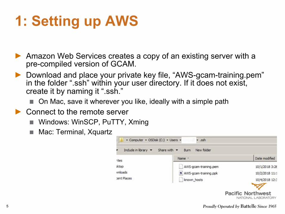
1: Setting up AWS

Amazon Web Services creates a copy of an existing server with a pre-compiled version of GCAM.Download and place your private key file, “AWS-gcam-training.pem” in the folder “.ssh” within your user directory. If it does not exist, create it by naming it “.ssh.”

On Mac, save it wherever you like, ideally with a simple path

Connect to the remote server Windows: WinSCP, PuTTY, XmingMac: Terminal, Xquartz

5

1: Configuring and Using WinSCP(Windows)

Host name: IP address of AWS serverPort: 22User Name: ec2-user

In advanced settings, open SSH -> Authentication. Use the browser “…” to find your private key file at “C:/Users/[username]/.ssh/”. When saved, WinSCP will automatically convert the .pem file to a .ppk file, readable by both WinSCP and PuTTY. Once logged in you will be able to interact with files and folders as in a system browser

6

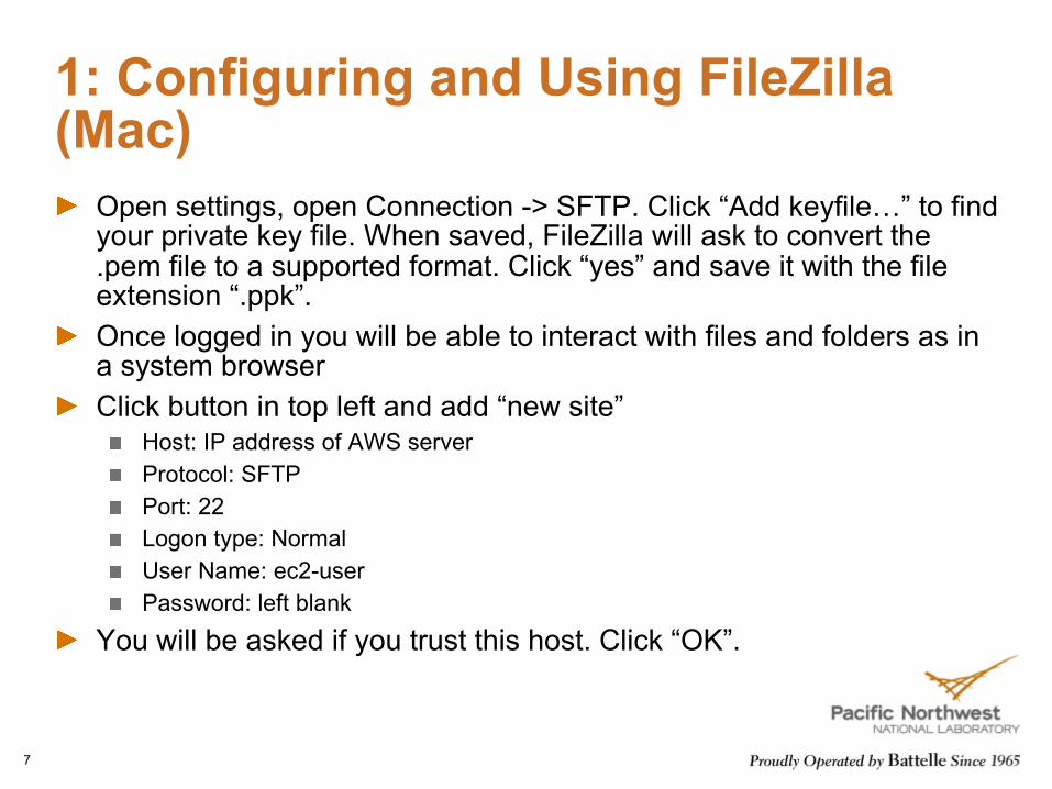
1: Configuring and Using FileZilla(Mac)

Open settings, open Connection -> SFTP. Click “Add keyfile…” to find your private key file. When saved, FileZilla will ask to convert the .pem file to a supported format. Click “yes” and save it with the file extension “.ppk”. Once logged in you will be able to interact with files and folders as in a system browserClick button in top left and add “new site”

Host: IP address of AWS serverProtocol: SFTPPort: 22Logon type: NormalUser Name: ec2-userPassword: left blank

You will be asked if you trust this host. Click “OK”.

7

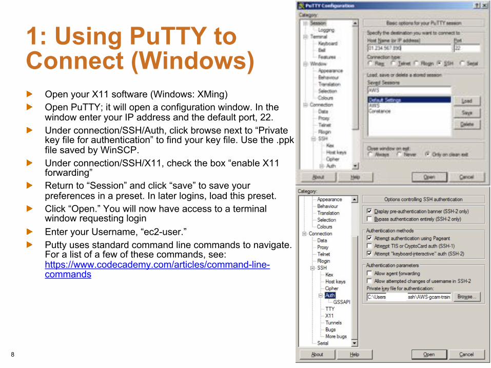
1: Using PuTTY to Connect (Windows)

Open your X11 software (Windows: XMing)Open PuTTY; it will open a configuration window. In the window enter your IP address and the default port, 22. Under connection/SSH/Auth, click browse next to “Private key file for authentication” to find your key file. Use the .ppkfile saved by WinSCP. Under connection/SSH/X11, check the box “enable X11 forwarding”Return to “Session” and click “save” to save your preferences in a preset. In later logins, load this preset.Click “Open.” You will now have access to a terminal window requesting loginEnter your Username, “ec2-user.”Putty uses standard command line commands to navigate. For a list of a few of these commands, see: https://www.codecademy.com/articles/command-line-commands

8

1: Using Terminal to Connect(Mac)

Open you X11 software (Xquartz)Open a terminal windowcd to the file location of your private key

(you can drag and drop the path into the terminal)Type “chmod 400 AWS-gcam-training.pem”. This sets your permissions so only you can see your private key. Only do this once.

Type in “ssh -Y -i AWS-gcam-training.pem ec2-user@xx.xxx.xxx.xxx”xx.xxx is the provided IP address of the AWS server

9

2: Running the Reference Scenario1) In your folder browser (WinSCP or FileZilla), navigate to the exe folder2) Open configuration_ref.xml

• This is a base configuration file that reads in files for the reference, or main, scenario

3) Save this as configuration.xml• This is the control file that is called when the model is run; the configuration.xml file

itself is usually over-written each time a new scenario is run. Configuration files that one wants to keep permanently should be saved under a different name

4) In your command line (Windows:PuTTY, Mac:Terminal), navigate to exe/ and run gcam.exe

1) Cd gcam/gcam5/exe/2) ./gcam.exe -Cconfiguration.xml

10

2: Configuration: the “Files” section

11

Base input file. ScenarioComponents append to this.For running multiple scenarios in sequence. Requires setting BatchMode bool to 1

For running climate target finder. Requires setting find-path bool to 1

* Write-output: indicate whether to create the file* Append-scenario-name: indicate whether to append the scenario name to the name of the file being created

xmldb is where the output will be saved

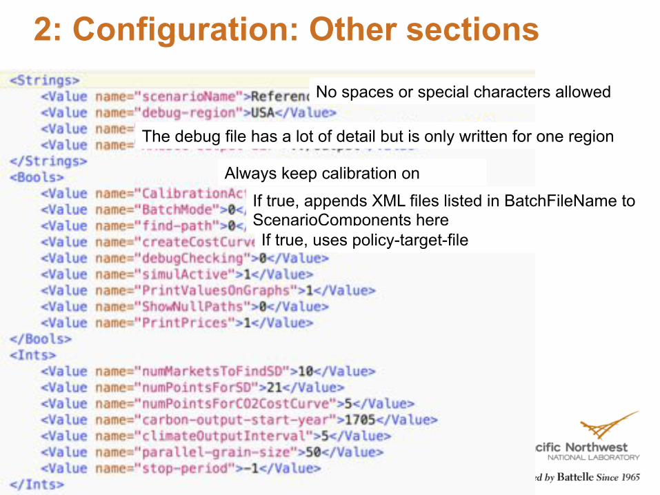
2: Configuration: Other sections

12

No spaces or special characters allowed

The debug file has a lot of detail but is only written for one region

Always keep calibration onIf true, appends XML files listed in BatchFileName to ScenarioComponents hereIf true, uses policy-target-file

2: Running GCAM

13

Command prompt/terminal window contains log messages

These are also written out to exe/logs/main_log.txt

Input files are read in the order that they appear in the configuration.exe file.

Where multiple files refer to the same parameter, the last one read in is the one whose value is used.

Recursive and dynamic: each period is solved independently, but information from one period is passed forward to the nextDeterministic: rerunning the model with no changes to input files will produce exactly the same outcome

2: OutputTwo forms of output

The output databaseoutput/database_basexdb (set in configuration.xml)Contains the results from the scenario in a database that can be queried

The debug fileexe/debugScenario.xml (filename set in config and merged with scenario name)

This writes out at the end of each time period, and contains a larger number of parameters for debuggingIt is only written for one region, set in the configuration file

14

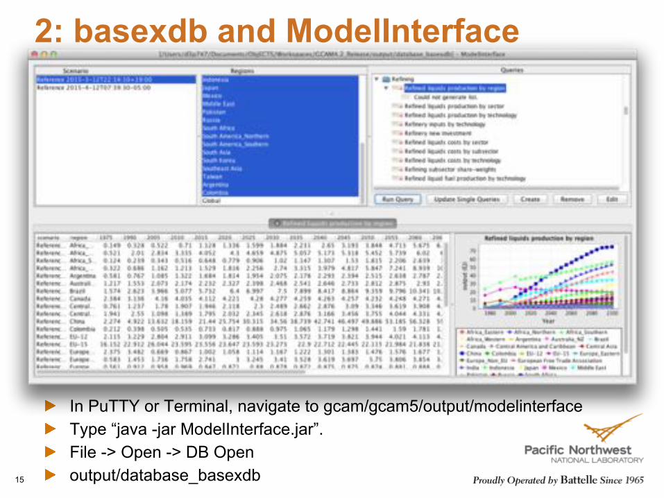
2: basexdb and ModelInterface

15

In PuTTY or Terminal, navigate to gcam/gcam5/output/modelinterface

Type “java -jar ModelInterface.jar”.

File -> Open -> DB Open

output/database_basexdb

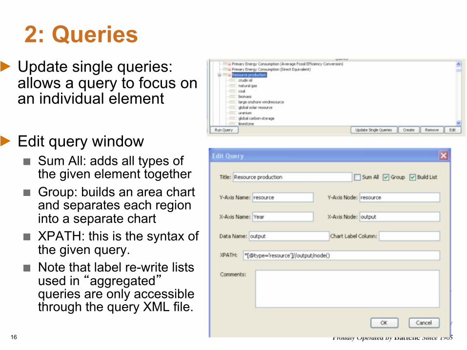
2: QueriesUpdate single queries: allows a query to focus on an individual element

Edit query windowSum All: adds all types of the given element togetherGroup: builds an area chart and separates each region into a separate chartXPATH: this is the syntax of the given query.Note that label re-write lists used in �aggregated�queries are only accessible through the query XML file.

16

2: Exporting dataHighlight cells, copy and pasteUse a batch query to export a large number of queries directly into an Excel spreadsheet

The dbxml file needs to be open for this to workFile -> Batch File. Select batch query file and output workbook.This won�t work if the Excel workbook selected is open while running the batch query

Drag and drop, e.g. into Excel (disabled in X11)

17

2: Exporting data with a batch query

18

Create a batch XML query file

and a blank XLS workbook

Open basexdb database first,

and then select File -> Batch

File

Select batch query file and XLS

workbook for export, making

sure that this workbook is

closed

This portion is pasted from model

interface queries, or Main_queries.xml

file. Only need to add region and aQuery

tags to make the batch query file.

2: Exporting, importing runs

File -> Manage DBThis allows one to rename, export (as an xml file, that can be imported into another .dbxml file), import, or remove a run from the databaseThe exported .xml files can also be useful for writing queries, as they contain all available information that could be queried

19

2: Useful Miscellaneous InfoAll energy flows are represented in EJ/yr. Note that the �year�denominator is implicit, not written out.Fuel carbon contents are in kgC/GJ.Emissions units

CO2 is in Mt C. Multiply by 44/12 to convert to CO2

Non-CO2 gases are generally in Tg (same as Mt). Exceptions are the hi-GWP gases (e.g. HFCs, PFCs, SF6), which are in Gg (same as kt).

Dollar unitsPrices of all energy goods and services are in 1975$/GJGDP is in 1990$/yrCarbon prices are in 1990$/tC. Multiply by 12/44 to convert to 1990$/tCO2.Fuel prices in policy scenarios do not include the emissions penalties. After converting to the desired dollar year, these may be added to any technology as:

C price ($/tC) * 1t / 1000kg * Fuel C content (kgC/GJ) * (1 –sequestration fraction)

20

3: Running alternative scenariosPretty much any study using GCAM will run alternative scenarios

Not an optimization model�Reference� scenario should not be seen as a most likely scenario, or even business as usual: it is only a starting point

Many possible variables of interest:Different technology RD&D futuresTechnology policies (e.g., standards, subsidies)CO2 and other GHG emissions pricingEmissions constraintsLand use policiesFuture energy prices or taxationDifferent population, GDP pathways

This section will focus on the provided policy files in the input/policy folder

21

3: Provided policy files

22

Carbon tax: exogenous CO2 price in each time period (1990$/t C)

Forcing target: radiative forcing (W/m2). Overshoot allows end-of-century target to be exceeded in prior years

FFICT: fossil fuel and industrial emissions only

UCT: universal (includes land use change emissions)

Input module: allows users to build XML files from excel

3: Configuration

23

Alternative scenarios may be run as follows:

add additional XML files at the end of the existing ScenarioComponentsChange the scenarioNameIndicate whether to use target-finder (if running an end-of-century climate target)Indicate whether to calculate abatement cost curves

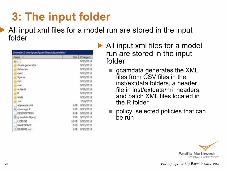
3: The input folderAll input xml files for a model run are stored in the input folder

24

All input xml files for a model run are stored in the input folder

gcamdata generates the XML files from CSV files in the inst/extdata folders, a header file in inst/extdata/mi_headers, and batch XML files located in the R folderpolicy: selected policies that can be run

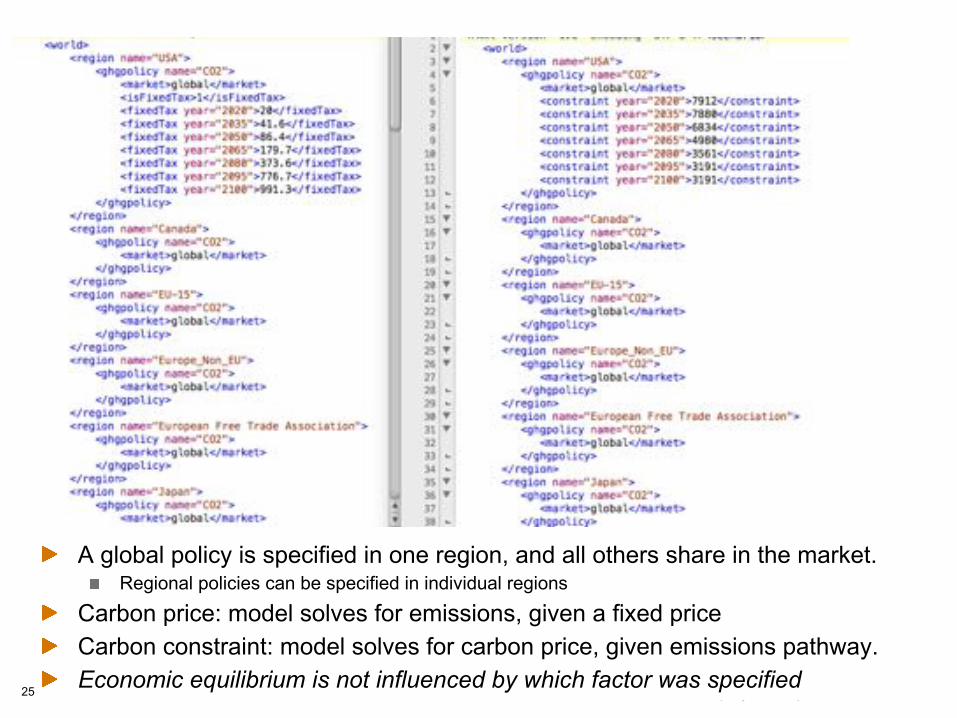
A global policy is specified in one region, and all others share in the market.Regional policies can be specified in individual regions

Carbon price: model solves for emissions, given a fixed priceCarbon constraint: model solves for carbon price, given emissions pathway.Economic equilibrium is not influenced by which factor was specified25

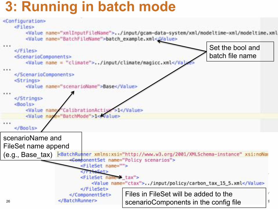
3: Running in batch mode

26

Set the bool and batch file name

scenarioName and FileSet name append (e.g., Base_tax)

Files in FileSet will be added to the scenarioComponents in the config file

4: DebuggingThis section will focus on the most common problemsIt will not attempt to cover everything that could happen, because there would be way too much to coverIt will proceed accordingly

1. Running the model2. Querying output3. Building XML files

27

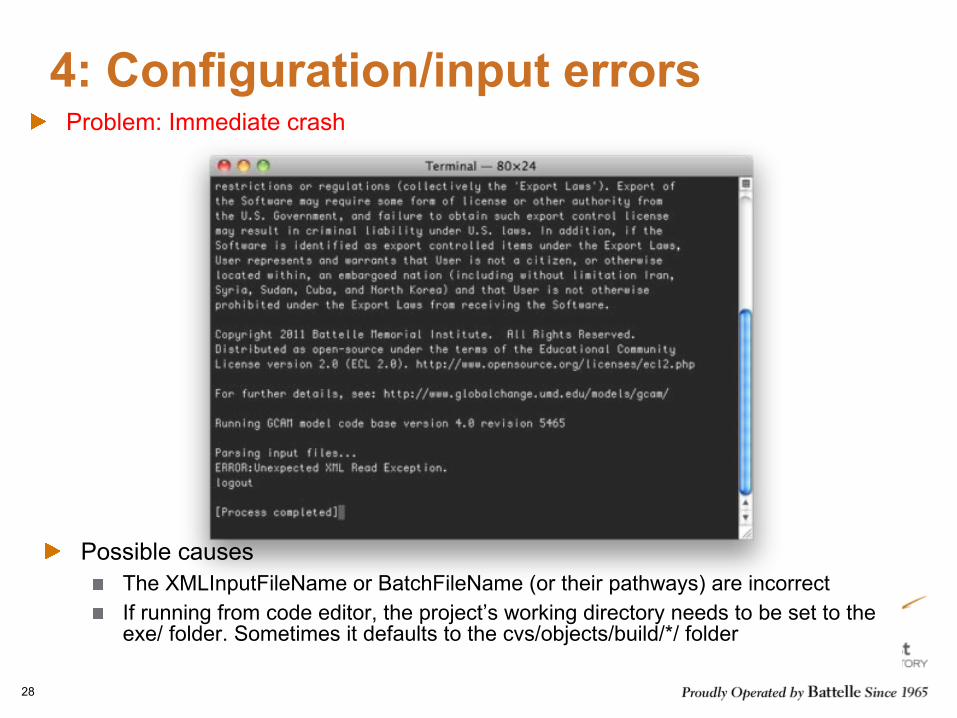
4: Configuration/input errors

28

Possible causesThe XMLInputFileName or BatchFileName (or their pathways) are incorrectIf running from code editor, the project’s working directory needs to be set to the exe/ folder. Sometimes it defaults to the cvs/objects/build/*/ folder

Problem: Immediate crash

4: Configuration/input errors

29

Problem: crash while reading in the ScenarioComponentsXML files

The problem: the last file read was mis-typed. Note the second �.xml�—this is a common error.

4: Configuration/input errors

30

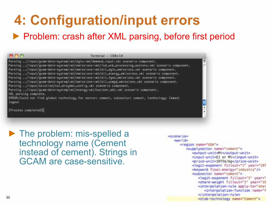
Problem: crash after XML parsing, before first period

The problem: mis-spelled a technology name (Cement instead of cement). Strings in GCAM are case-sensitive.

4: Errors from changes to input files

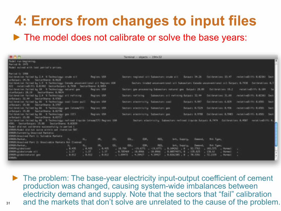
31

The model does not calibrate or solve the base years:

The problem: The base-year electricity input-output coefficient of cement production was changed, causing system-wide imbalances between electricity demand and supply. Note that the sectors that “fail” calibration and the markets that don’t solve are unrelated to the cause of the problem.

4: Model not solving with policyThe model fails to solve in some period

32

The problem: An extremely high carbon tax ($25,000/tC) was implemented in 2020. Solution failure is more likely with carbon emissions constraints than taxes, particularly if land use change emissions are included in the cap.

4: Database open while trying to writeThe model can’t write to the output database

33

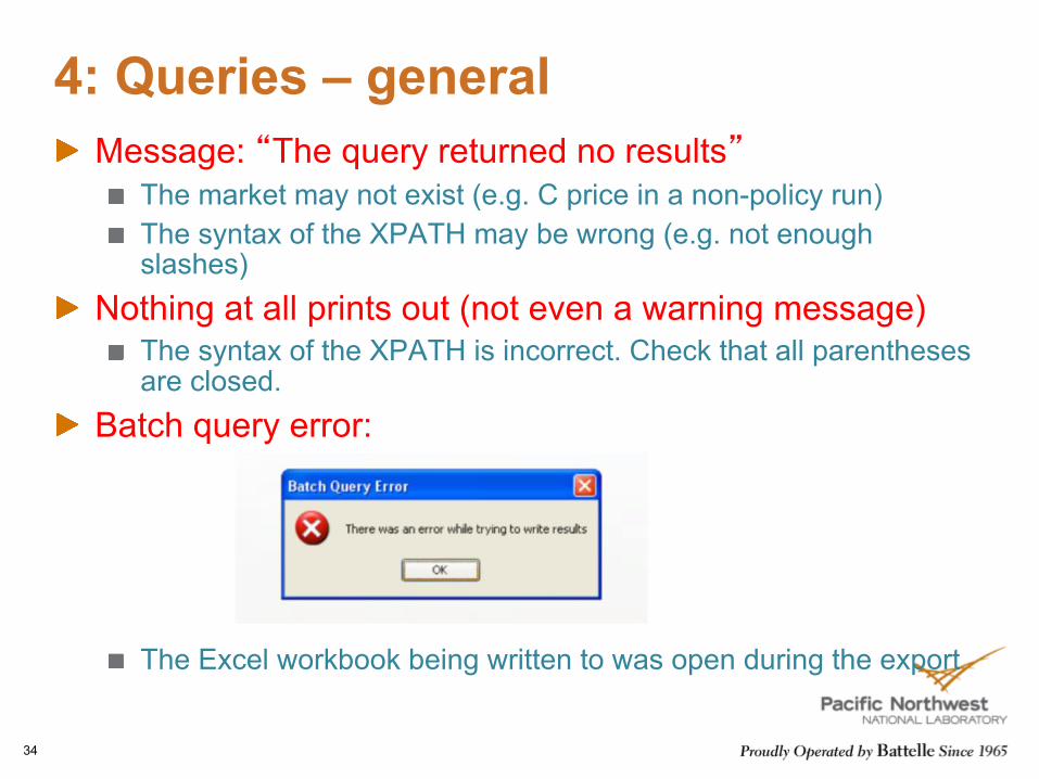
4: Queries – generalMessage: �The query returned no results�

The market may not exist (e.g. C price in a non-policy run)The syntax of the XPATH may be wrong (e.g. not enough slashes)

Nothing at all prints out (not even a warning message)The syntax of the XPATH is incorrect. Check that all parentheses are closed.

Batch query error:

The Excel workbook being written to was open during the export

34

4: Building XML files - general

35

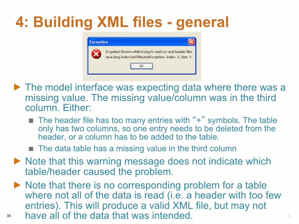
The model interface was expecting data where there was a missing value. The missing value/column was in the third column. Either:

The header file has too many entries with �+� symbols. The table only has two columns, so one entry needs to be deleted from the header, or a column has to be added to the table.The data table has a missing value in the third column

Note that this warning message does not indicate which table/header caused the problem.Note that there is no corresponding problem for a table where not all of the data is read (i.e. a header with too few entries). This will produce a valid XML file, but may not have all of the data that was intended.

4: Building XML files - general

36

There is a header in the headers file that doesn�t have the following entry:,scenario,

5: What does it all mean?This section focuses on the meaning of several key input parameters found throughout the input XML file set

ElasticitiesLogit exponentsShare-weights and interpolation rulesEfficiencies and coefficients

37

5: ElasticityPrice elasticity: The percent change in demand of a good divided by the percent change in the priceIncome elasticity: The percent change in demand of a good divided by the percent change in GDP

38

elasptelasinctiti P

PGDPGDPDD -- ••= )()(

200520052005,,

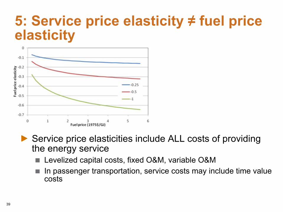
5: Service price elasticity ≠ fuel price elasticity

Service price elasticities include ALL costs of providing the energy service

Levelized capital costs, fixed O&M, variable O&MIn passenger transportation, service costs may include time value costs

39

5: Logit-exponents and fuel-switching

The logit exponents control the degree of switching between technologies or fuels in response to price changes

Low values = low fuel-switching = strong influence of base year shares even far into the futureHigh values tend towards winner-take-all responses in response to changes in costs

40

å •

•=

iii

iii Psw

PswShare b

b

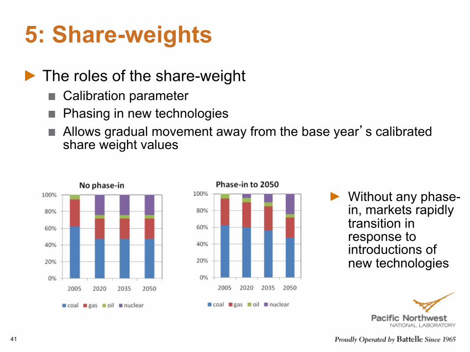
5: Share-weightsThe roles of the share-weight

Calibration parameterPhasing in new technologiesAllows gradual movement away from the base year�s calibrated share weight values

41

Without any phase-in, markets rapidly transition in response to introductions of new technologies

5: Efficiencies and coefficients

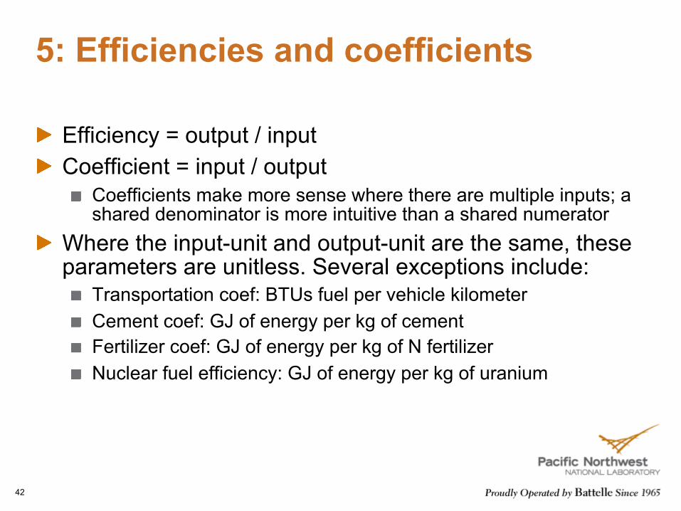
Efficiency = output / inputCoefficient = input / output

Coefficients make more sense where there are multiple inputs; a shared denominator is more intuitive than a shared numerator

Where the input-unit and output-unit are the same, these parameters are unitless. Several exceptions include:

Transportation coef: BTUs fuel per vehicle kilometerCement coef: GJ of energy per kg of cementFertilizer coef: GJ of energy per kg of N fertilizerNuclear fuel efficiency: GJ of energy per kg of uranium

42

5: InterpolationInterpolation is primarily used for defining share-weight pathways into the future

Fixed: carry the shareweight in the “from-year” to the “to-year” with no changes. Requires a from-value.Linear: linearly interpolate. Requires a from-value and a to-value, which can be set within the interpolation rule, or in the share-weight parameter.S-curve: s-curve shaped function. Requires a from-value and a to-value. Note that the to-year doesn’t need to be a model time period, but if it isn’t, need to set the “to-value” within the rule.

43

Appendix

44

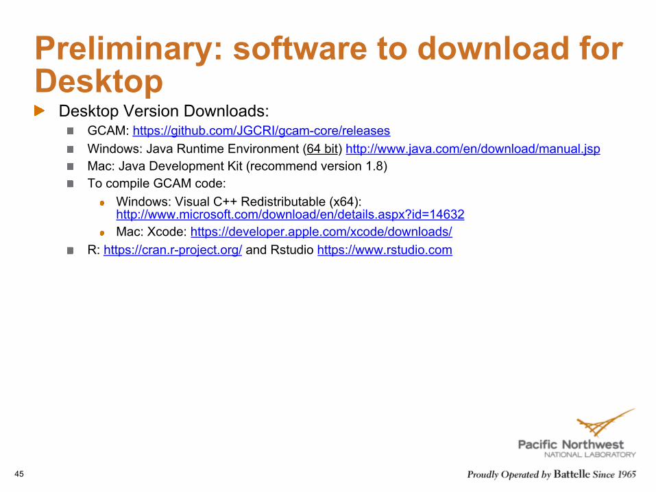
Preliminary: software to download for Desktop

Desktop Version Downloads:GCAM: https://github.com/JGCRI/gcam-core/releasesWindows: Java Runtime Environment (64 bit) http://www.java.com/en/download/manual.jspMac: Java Development Kit (recommend version 1.8)To compile GCAM code:

Windows: Visual C++ Redistributable (x64): http://www.microsoft.com/download/en/details.aspx?id=14632Mac: Xcode: https://developer.apple.com/xcode/downloads/

R: https://cran.r-project.org/ and Rstudio https://www.rstudio.com

45

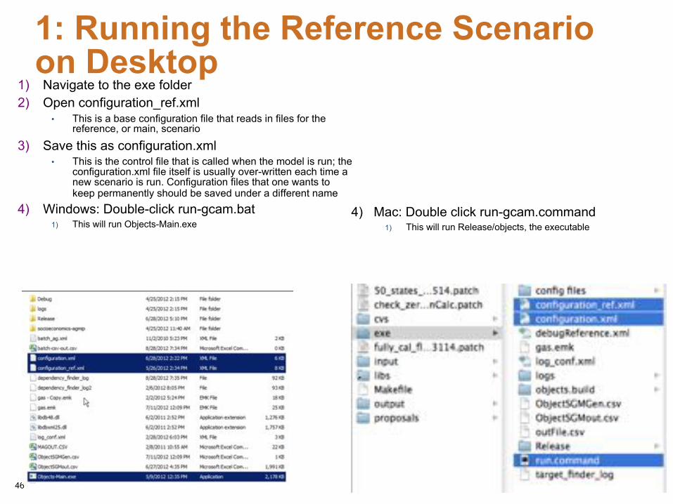
1: Running the Reference Scenario on Desktop

1) Navigate to the exe folder2) Open configuration_ref.xml

• This is a base configuration file that reads in files for the reference, or main, scenario

3) Save this as configuration.xml• This is the control file that is called when the model is run; the

configuration.xml file itself is usually over-written each time a new scenario is run. Configuration files that one wants to keep permanently should be saved under a different name

4) Windows: Double-click run-gcam.bat1) This will run Objects-Main.exe

46

4) Mac: Double click run-gcam.command1) This will run Release/objects, the executable

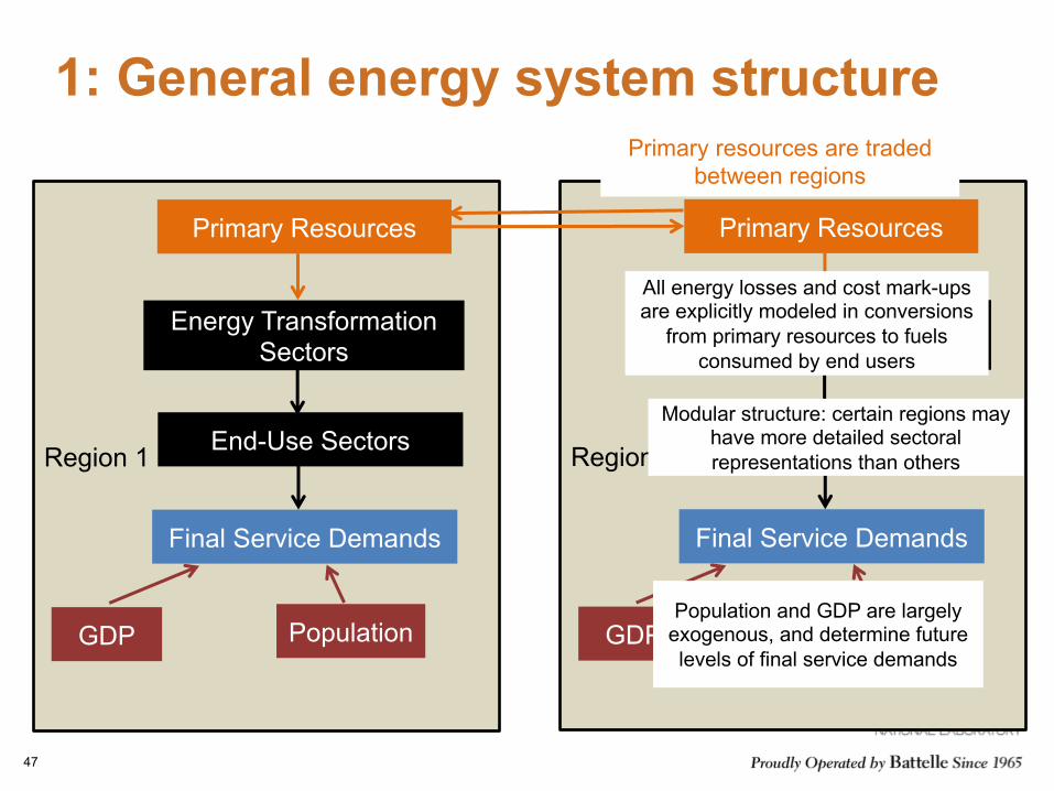
1: General energy system structure

47

Region 1

Energy Transformation Sectors

Primary Resources

End-Use Sectors

Final Service Demands

GDP Population

Region 2

Energy Transformation Sectors

Primary Resources

End-Use Sectors

Final Service Demands

GDP Population

Primary resources are traded between regions

All energy losses and cost mark-ups are explicitly modeled in conversions

from primary resources to fuels consumed by end users

Modular structure: certain regions may have more detailed sectoralrepresentations than others

Population and GDP are largely exogenous, and determine future levels of final service demands

1: General energy system structure

48

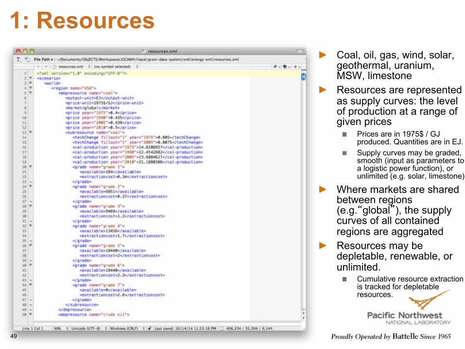
1: ResourcesCoal, oil, gas, wind, solar, geothermal, uranium, MSW, limestoneResources are represented as supply curves: the level of production at a range of given prices

Prices are in 1975$ / GJ produced. Quantities are in EJ.Supply curves may be graded, smooth (input as parameters to a logistic power function), or unlimited (e.g. solar, limestone)

Where markets are shared between regions (e.g.�global�), the supply curves of all contained regions are aggregatedResources may be depletable, renewable, or unlimited.

Cumulative resource extraction is tracked for depletableresources.

49

1: Domestic energy supplyen_supply.xmlDomestic energy supply =

Sum of all consumption within a regionProduction minus net exports

These are generally uncalibrated “pass-through sectors” used for tracking purposesThey can be used to implement region-specific energy price adders or subsidies

We currently apply the same cost adders in all regions in order to remain flexible to energy system changes in the futureRegional energy prices are not currently calibrated; instead, regional fuel prices are implicitly captured in the derived calibration parameters

50

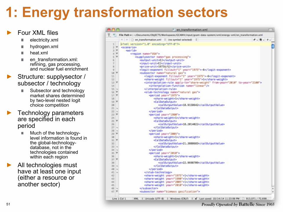
1: Energy transformation sectorsFour XML files

electricity.xmlhydrogen.xmlheat.xmlen_transformation.xml: refining, gas processing, and nuclear fuel enrichment

Structure: supplysector / subsector / technology

Subsector and technology market shares determined by two-level nested logitchoice competition

Technology parameters are specified in each period

Much of the technology-level information is found in the global-technology-database, not in the technologies contained within each region

All technologies must have at least one input (either a resource or another sector)

51

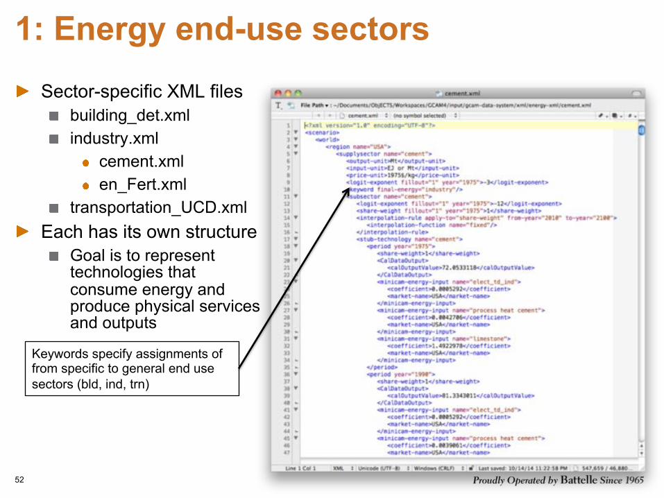
1: Energy end-use sectorsSector-specific XML files

building_det.xmlindustry.xml

cement.xmlen_Fert.xml

transportation_UCD.xmlEach has its own structure

Goal is to represent technologies that consume energy and produce physical services and outputs

52

Keywords specify assignments of from specific to general end use sectors (bld, ind, trn)

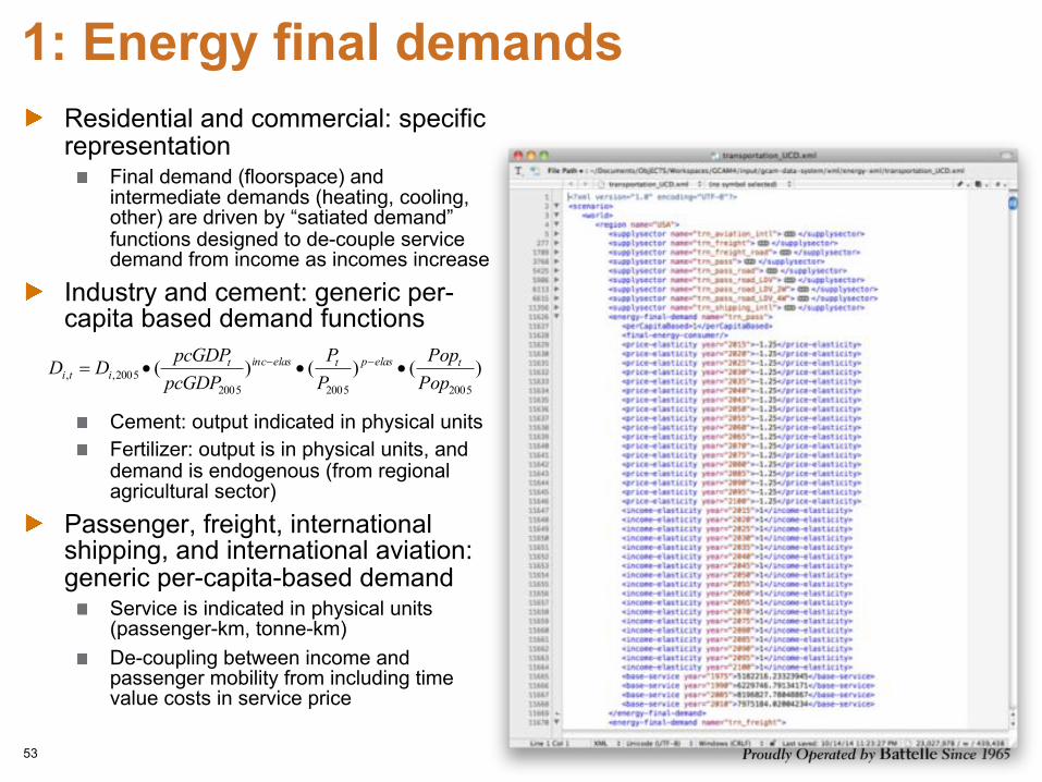
1: Energy final demandsResidential and commercial: specific representation

Final demand (floorspace) and intermediate demands (heating, cooling, other) are driven by “satiated demand” functions designed to de-couple service demand from income as incomes increase

Industry and cement: generic per-capita based demand functions

Cement: output indicated in physical unitsFertilizer: output is in physical units, and demand is endogenous (from regional agricultural sector)

Passenger, freight, international shipping, and international aviation: generic per-capita-based demand

Service is indicated in physical units (passenger-km, tonne-km)De-coupling between income and passenger mobility from including time value costs in service price

53

)()()(200520052005

2005,, PopPop

PP

pcGDPpcGDPDD telasptelasinct

iti •••= --

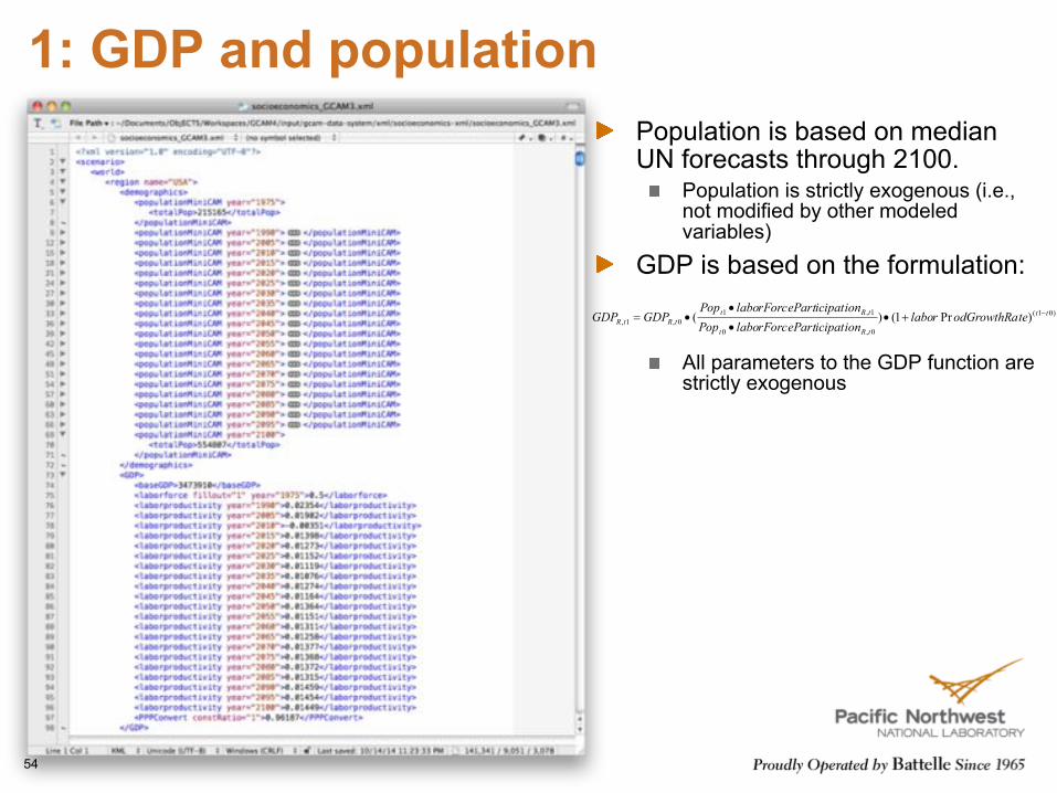
1: GDP and populationPopulation is based on median UN forecasts through 2100.

Population is strictly exogenous (i.e., not modified by other modeled variables)

GDP is based on the formulation:

All parameters to the GDP function are strictly exogenous

54

)01(

0,0

1,10,1, )Pr1()( tt

tRt

tRttRtR teodGrowthRalabor

ionParticipatlaborForcePopionParticipatlaborForcePop

GDPGDP -+••

••=

1: Non-CO2 gasesNon-CO2 gases are modeled as a by-product on existing activities, either driven by �input� (e.g. fuel consumption) or �output� (e.g. service or energy production)

55

Can be read in as input-emissions (Tg/yr) or as emissions coefficients (kg/GJ)GDP control function: emissions coefficients are reduced as GDP increasesMAC = marginal abatement cost curve; decreases coefficients as carbon price increases.

Coeft1 =Coeft0 •(1−min(maxReduction,1−1

1+ (pcGDPt1 − pcGDPt0 )Steepness

)

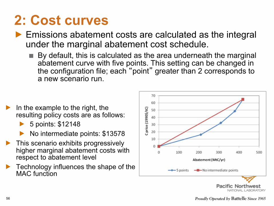
2: Cost curvesEmissions abatement costs are calculated as the integral under the marginal abatement cost schedule.

By default, this is calculated as the area underneath the marginal abatement curve with five points. This setting can be changed in the configuration file; each �point� greater than 2 corresponds to a new scenario run.

56

In the example to the right, the resulting policy costs are as follows:

5 points: $12148No intermediate points: $13578

This scenario exhibits progressively higher marginal abatement costs with respect to abatement levelTechnology influences the shape of the MAC function

Adjusting queriesChanges can be made in the Main_queries.xml file, or by opening up a database in the model GUI

Note that label re-write lists for aggregated queries can not be accessed from the model GUIX-Axis name is almost always year; y-axis name is the same as the series name.XPATH has the specific query instructions

57

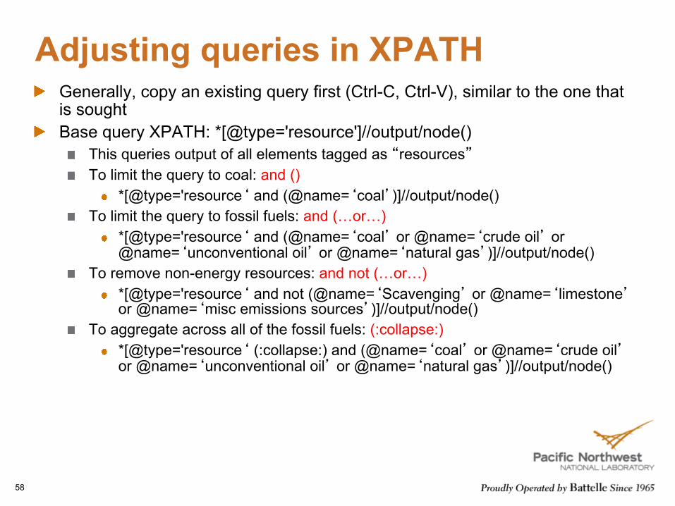
Adjusting queries in XPATHGenerally, copy an existing query first (Ctrl-C, Ctrl-V), similar to the one that is soughtBase query XPATH: *[@type='resource']//output/node()

This queries output of all elements tagged as �resources�To limit the query to coal: and ()

*[@type='resource� and (@name=�coal�)]//output/node()To limit the query to fossil fuels: and (…or…)

*[@type='resource� and (@name=�coal� or @name=�crude oil� or @name=�unconventional oil� or @name=�natural gas�)]//output/node()

To remove non-energy resources: and not (…or…)*[@type='resource� and not (@name=�Scavenging� or @name=�limestone�or @name=�misc emissions sources�)]//output/node()

To aggregate across all of the fossil fuels: (:collapse:)*[@type='resource� (:collapse:) and (@name=�coal� or @name=�crude oil�or @name=�unconventional oil� or @name=�natural gas�)]//output/node()

58

Adjusting queries in XPATH

Where information is low in a heirarchy, one can choose how many levels of the heirarchy to show in the output:Base query XPATH: *[@type = 'sector' and ((@name='gas processing') )]//*[@type = 'technology']/*[@type='output' (:collapse:)]/physical-output/node()

The double slash (//*) indicates to go down by more than one levelTo also write out the subsector: only one /**[@type = 'sector' and ((@name='gas processing') )] /*[@type = 'subsector']/*[@type = 'technology']/*[@type='output' (:collapse:)]/physical-output/node()

59

Gas production by technologyscenario region sector technology 1990 2005 2020Main,date=2010-23-9T12:05:21-04:00 USA gas processing biomass gasification 0.031 0.160 0.159Main,date=2010-23-9T12:05:21-04:00 USA gas processing coal gasification 0.136 0.046 0.067Main,date=2010-23-9T12:05:21-04:00 USA gas processing natural gas 18.267 21.692 23.517

Gas production by technology

scenario region sector subsector technology 1990 2005 2020

Main,date=2010-23-9T12:05:21-04:00 USA gas processing biomass gasification biomass gasification 0.031 0.160 0.159

Main,date=2010-23-9T12:05:21-04:00 USA gas processing coal gasification coal gasification 0.136 0.046 0.067

Main,date=2010-23-9T12:05:21-04:00 USA gas processing natural gas natural gas 18.267 21.692 23.517

2: Running the diagnostics package

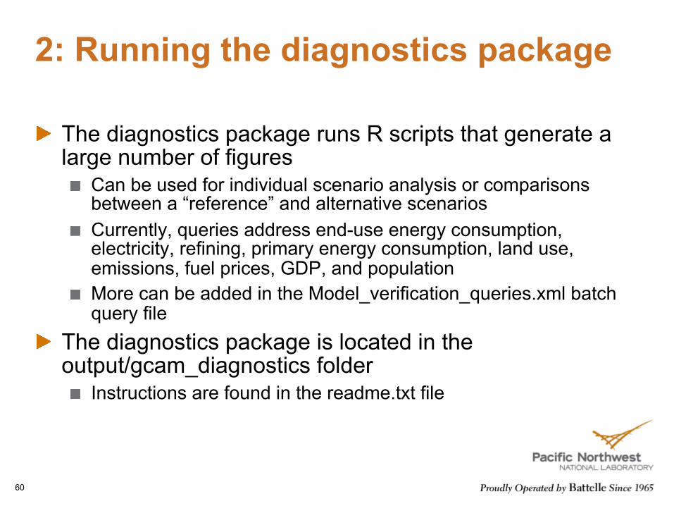
The diagnostics package runs R scripts that generate a large number of figures

Can be used for individual scenario analysis or comparisons between a “reference” and alternative scenariosCurrently, queries address end-use energy consumption, electricity, refining, primary energy consumption, land use, emissions, fuel prices, GDP, and populationMore can be added in the Model_verification_queries.xml batch query file

The diagnostics package is located in the output/gcam_diagnostics folder

Instructions are found in the readme.txt file

60

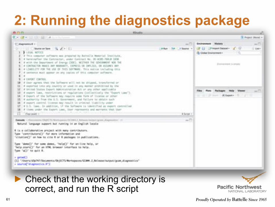
2: Running the diagnostics package

61

Check that the working directory is correct, and run the R script

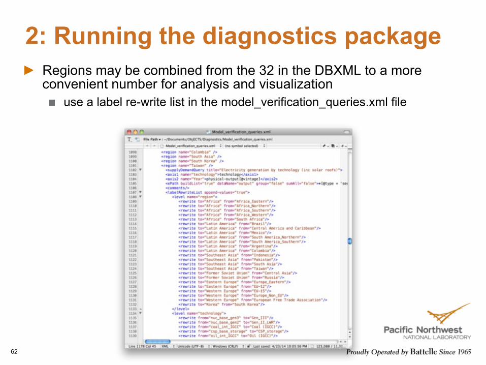
2: Running the diagnostics packageRegions may be combined from the 32 in the DBXML to a more convenient number for analysis and visualization

use a label re-write list in the model_verification_queries.xml file

62

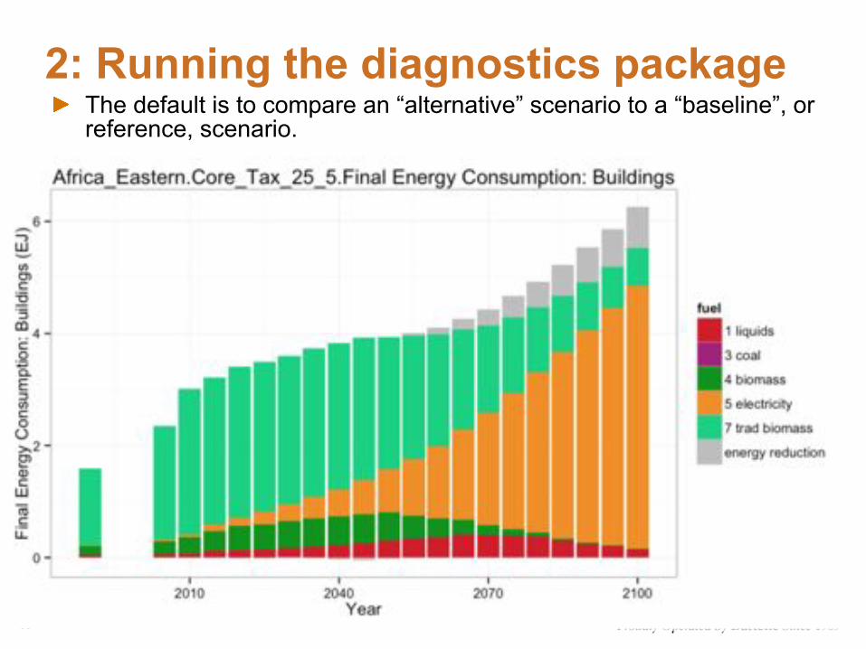
2: Running the diagnostics packageThe default is to compare an “alternative” scenario to a “baseline”, or reference, scenario.

63