GLM models and OLS regression

Graeme Hutcheson, University of Manchester

The lecture notes, exercises and data sets associated with this course are available for downloadfrom:

www.Research-Training.net/Manchester

This session introduces the ordinary least-squares regression model which can be used to modelcontinuous variables. We cover the theory behind the technique, the interpretation of the parametersand confidence intervals and also the computation and interpretation of the model-fit statistics.Where appropriate, code for Rcmdr is included to enable the analyses and graphics to be reproduced.

OLS regression is a particularly important technique not only because it provides a method ofmodeling continuous data, but also because it is central to understanding the wider application ofthe generalised linear model to other types of data.

1 The Generalized Linear Model

This chapter introduces generalized linear models (GLMs) and shows how they can be used to modelcontinuous, ordered and unordered data (the three basic scales of data described in Chapter 1). Theobject is to provide a coherent introduction to data modeling rather than provide a comprehensivecoverage of all techniques under the GLM umbrella. GLMs enable descriptive and predictive modelsto be built that are sufficiently general to be applicable to much social science data. They can beused to model data collected from survey and experimental studies and can replace many of themore traditional hypothesis tests that are still in common use. Of particular importance is theunified theoretical framework that the method offers, as this enables certain ‘economies of scale’ tobe realised that allow a whole range of data to be analysed using similar techniques.

The use of the techniques will be described using a modeling procedure whereby a particular variablecan be modeled (or predicted) using information about other variables. For example,

Variable Y may be predicted by Variable X1 and Variable X2.

Variable Y (the variable that is being modeled — the response variable) could be wage, educationalattainment, test score, share price, a binary category indicating success and failure, University cho-sen or religious affiliation. Variables X1 and X2 (the variables used to predict Y — the explanatoryvariables) could be age, average school grade, gender, nationality, race, attractiveness, weight, atti-tude to innovation or treatment group. In short, variables Y , X1 and X2 can be recorded on any ofthe scales described in Chapter One. Using the concrete example of a particular company’s shareprice, the relationship above can be written as:

Share Price may be predicted by Output and Market Confidence.

From the relationship above one can deduce that share price may be determined by the company’soutput and the confidence shown in the market the company operates in. This is not likely to be aperfect relationship as a number of other variables not represented in the model will also influenceshare price (such as government policy and exchange rates). In general, for the model above, highoutput and high market confidence is likely to be associated with a relatively high share price(although this might not always be the case). The model can be said to consist of three components,the response variable, Y , the explanatory variables, X1 and X2 and a function that links the two.These three components form the basis of the Generalized Linear Model where they are commonlyreferred to as the random component, the systematic component and the link function.

• The random component:

the probability distribution assumed to underlie the response variable.

• The systematic component:

the fixed structure of the explanatory variables, usually characterised by a linear function(α+ β1x1 + β2x2 + β3x3 + ...+ βkxk).

• The link function:

the function that maps the systematic component onto the random component. This functioncan be one of identity for Normally distributed random components, or one of a number ofnon-linear links when the random component is not Normally distributed.

The GLM can be summarised as:

RandomComponent

-Link

Function

SystematicComponent

with a concrete example being:

Share Price -Link

Function

Output

and

Market Confidence

The probability distribution assumed to underlie the random component is a function of the data.For example, when the response variable is continuous, a Normal distribution may be used, whereasa binomial distribution may be used when the response variable is dichotomous. The link function isalso dependent on the scale in which the response variable is recorded. For example, for a Normally-distributed response variable, the relationship between the random and systematic components isone of identity (=), where the random component actually equals the systematic component. For abinomially distributed response variable, the link between the random and systematic componentsis the log odds, or logit, and for count data it is the log. These can be seen in Rcmdr as the defaultlinks for the guassian, binomial and poisson families of random components.

We introduce generalized linear models using Ordinary Least-Squares regression (OLS), a techniquethat can be used to model a continuous response variable.

2

Figure 1: Models that can be fit under the Statistics, Fit models, Generalized liner model...menu tree in Rcmdr . Note that the default link function changes depending on the response variable.For the continuous model shown in the top-left, the response variable is continuous and the defaultlink is the identity (=). For the categorical model shown on the bottom, the response variable iscategorical and the default link is the logit (log-odds). For the count data model shown on the right,the response variable is count data and the default link shown for this is a log-link (a log-linearmodel).

2 Modelling a continuous variable

A continuous response variable (a variable that can legitimately be described using the mean) canbe modeled using ordinary least-squares (OLS) regression, one of the GLM modeling techniques.We will describe the theory and application of the technique in relation to a simple data set andbuild from a simple to a multi-variable model that includes categorical explanatory variables. Thedata that are to be used here to illustrate the technique are from Koteswara, 1970, (reported inHand et al., 1994) who presents data collected over 30 four-week periods from March 18th 1951 toJuly 11th 1953. The data show ice cream consumption (pints per capita), the price of ice cream(in dollars per pint), the weekly family income (in dollars) and the mean outdoor temperature (indegrees Fahrenheit). These data are shown in Table 1.

Table 1: Data: Ice cream consumption

Ice Cream Price Family TemperatureConsumption Income

.386 .270 78 41

.374 .282 79 56

.393 .277 81 63

.425 .280 80 68

.406 .272 76 69

.344 .262 78 65

continued on next page . . .

3

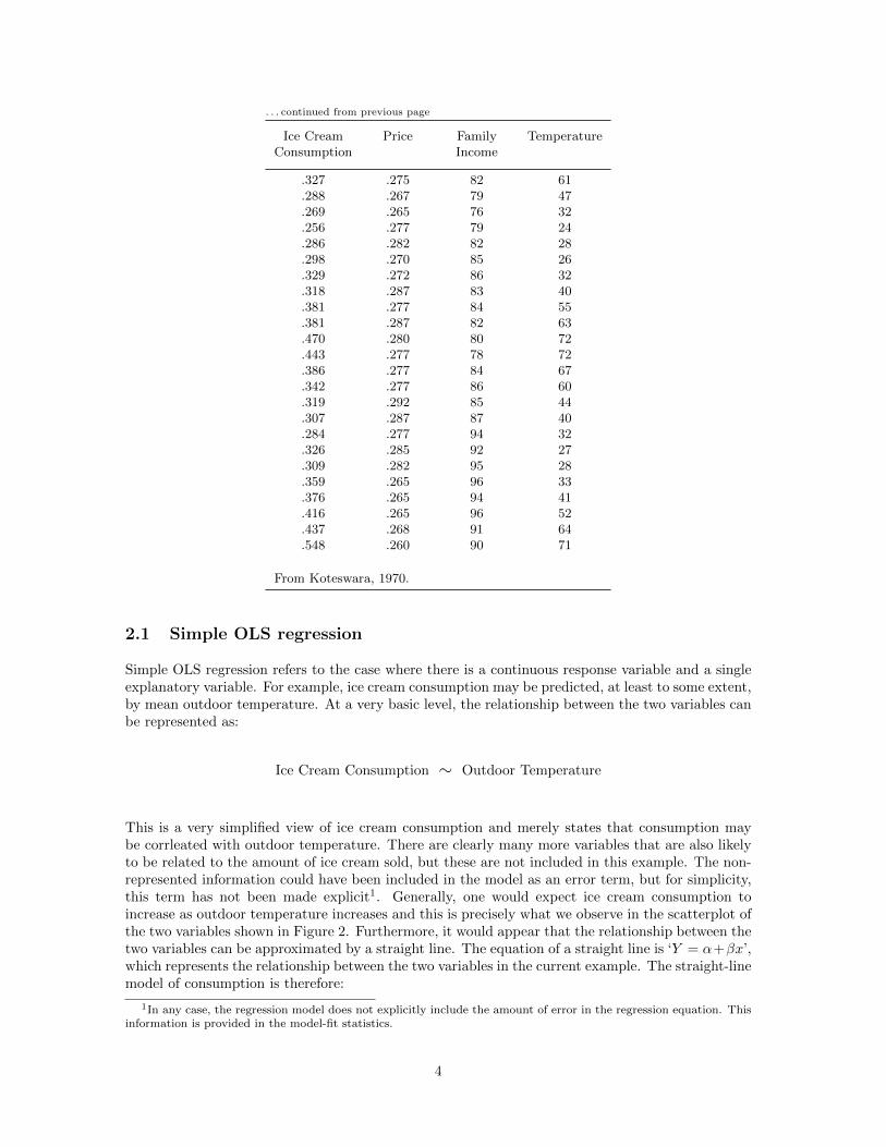
. . . continued from previous page

Ice Cream Price Family TemperatureConsumption Income

.327 .275 82 61

.288 .267 79 47

.269 .265 76 32

.256 .277 79 24

.286 .282 82 28

.298 .270 85 26

.329 .272 86 32

.318 .287 83 40

.381 .277 84 55

.381 .287 82 63

.470 .280 80 72

.443 .277 78 72

.386 .277 84 67

.342 .277 86 60

.319 .292 85 44

.307 .287 87 40

.284 .277 94 32

.326 .285 92 27

.309 .282 95 28

.359 .265 96 33

.376 .265 94 41

.416 .265 96 52

.437 .268 91 64

.548 .260 90 71

From Koteswara, 1970.

2.1 Simple OLS regression

Simple OLS regression refers to the case where there is a continuous response variable and a singleexplanatory variable. For example, ice cream consumption may be predicted, at least to some extent,by mean outdoor temperature. At a very basic level, the relationship between the two variables canbe represented as:

Ice Cream Consumption ∼ Outdoor Temperature

This is a very simplified view of ice cream consumption and merely states that consumption maybe corrleated with outdoor temperature. There are clearly many more variables that are also likelyto be related to the amount of ice cream sold, but these are not included in this example. The non-represented information could have been included in the model as an error term, but for simplicity,this term has not been made explicit1. Generally, one would expect ice cream consumption toincrease as outdoor temperature increases and this is precisely what we observe in the scatterplot ofthe two variables shown in Figure 2. Furthermore, it would appear that the relationship between thetwo variables can be approximated by a straight line. The equation of a straight line is ‘Y = α+βx’,which represents the relationship between the two variables in the current example. The straight-linemodel of consumption is therefore:

1In any case, the regression model does not explicitly include the amount of error in the regression equation. Thisinformation is provided in the model-fit statistics.

4

Figure 2: A scatter-plot showing the relationship between ice cream consumption and outdoortemperature. The straight line is the OLS regression model consumption = α+ β temperature.

consumption = α+ β temperature (1)

2.1.1 computing and interpreting model parameters

The relationship between the response variable (consumption) and the explanatory variable (tem-perature) may be represented by a straight line and can therefore be given in the form ‘Y = α+βx’.This linear model is derived using an algorithm that minimises the sum of the squares of the dis-tances from each data point to the line (hence it is known as the least-squares technique) producinga line of best-fit (the straight line drawn on the graph in Figure 2). Readily available statisticalsoftware can compute the model parameters for the model ‘consumption = α + β temperature’ andthese are shown in Table 2. From the estimates provided in this table, one can obtain the intercept(α) and the regression coefficient for temperature (β) to get the equation of the line of best-fit, whichis

consumption = 0.207 + (0.003 ∗ temperature). (2)

The estimate for the variable ‘temperature’ indicates that for each unit increase in temperature, percapita consumption of ice cream is expected to increase by 0.003 pints. This increase in ice creamconsumption is the average increase one would expect2.

2The estimate for the intercept is not all that informative in this case as it just indicates the consumption whenthe temperature is zero (as we do not know if a linear model holds for temperatures this low, interpreting this valueis often futile).

5

Table 2: Regression parameters

estimate standard error

(intercept) 0.207 0.0247temperature 0.003 0.0005

Model: consumption = α + β temperature

It is useful to also determine the limits within which one might expect consumption to change givena unit increase in temperature (i.e., how accurate the β parameter is). These limits are known asconfidence intervals and may be calculated using Equation 3.

Large sample 95% confidence interval for β = β ± 1.96(s.e. β) (3)

where β indicates that β is estimated from the data.

For the model above,

Large sample 95% confidence interval for β = 0.003± (1.96× 0.0005)

= 0.002, 0.004

In 95% of cases, the expected increase in per capita consumption of ice cream for each degree risein temperature is between 0.002 and 0.004 pints per capita. In other words, for a unit increase intemperature (a one degree rise) in 95% of cases one would expect consumption to increase by atleast 0.002 pints per capita but not more than 0.004 pints per capita. As both of these confidenceintervals predict an increase in the consumption of ice cream, we can conclude that at the 95%two-tailed level of significance, ‘temperature’ does have a significant affect on the response variable(this is confirmed in the next section when the model-fit statistics are discussed).

2.1.2 predicting the response variable

From the model provided above in Equation 2, it is a simple matter to obtain predictions for theresponse variable at any given value of temperature (provided that it is within the range of obser-vations recorded during the study). For example, when the temperature is 50 degrees Fahrenheit,ice cream consumption is predicted to be

consumption = 0.207 + (0.003 ∗ 50)

= 0.357

which can be confirmed by looking at the graph of the regression model in Figure 2. It is aneasy matter to compute these predictions using software. Table 3 shows predicted probabilities ofice cream consumption for a number of different temperatures computed using the R statistical

6

Table 3: Predictions of consumption

temperature predicted consumption

41 0.33456 0.38163 0.40368 0.41869 0.42165 0.40961 0.39647 0.35332 0.30624 0.28128 0.294

Model: consumption = 0.207 + (0.003 * temperature)

package. From the predicted values in the table, it is easy to see that the predicted consumptionincreases with temperature.

The R commands for plotting the prediction intervals are shown at the end of this document alongwith a graph showing the confodence intervals for the mean prediction and also the predictionintervals for individual predictions.

2.1.3 goodness of fit statistics

In addition to the model parameters and confidence intervals, it is useful to have an indication ofhow well the model fits the data. For this we need to compute some model-fit statistics. How wellthe model fits the data can be determined by comparing the observed scores (the data) with thosepredicted from the model. The difference between these two values (the deviation or residual, asthey are sometimes called) provides an indication of how well the model predicts each data point.Adding up the deviances for all the data points after they have been squared (in order to removeany negative values) provides a measure of how much the data deviates from the model overall.The sum of all the squared residuals is known as the residual sum of squares (RSS) and essentiallyprovides a measure of model-fit. A poorly fitting model will deviate markedly from the data and willconsequently have a relatively large RSS, whereas a good-fitting model will not deviate markedlyfrom the data and will consequently have a relatively small RSS (a perfectly fitting model will havean RSS equal to zero, as there will be no deviation). The RSS statistic therefore provides a measureof model-fit and can be used to determine the significance of individual and groups of parametersfor a regression model. This statistic is also known as the deviance and is discussed in depth byAgresti, 1996 (pages 96–97).

A ‘model’ computed for a single continuous response variable, Y, has the form ‘Y = α’, where α isequal to the mean value (if the only information you have about a continuous variable is the variableitself, the best prediction you can make about its value is the mean value). The residuals for sucha model are simply the difference between each data point and the mean of the distribution (thepredicted value from the model, designated as x). The deviance in the model can be computed byadding up all of the squared residuals for each data point as defined in Equation 4 and illustratedfor the variable consumption in Figure 3.

7

deviance = (x1 − x)2 + (x2 − x)2 + ....+ (xk − x)2 (4)

Figure 3: Residuals for the model ‘consumption = α’

Table 4 shows the residuals and squared residuals for each consumption data point. These residualshave been calculated by simply subtracting the mean value of consumption (0.3594) from each ofthe observed values (xi − x). Adding up all of the squared residuals provides the deviance for themodel ‘consumption = α’, which is calculated as 0.1255.

The deviance can also be derived for models that include one or more explanatory variables. Figure4 gives a visual representation of how the residuals are calculated for the simple regression model‘consumption = α + β temperature’. The residuals are calculated as the distances from each datapoint to the regression line (rather than to the average value) and these are clearly shown in thediagram. For a comprehensive illustration of modeling relationships and determining residual scoresfor simple regression models, see Miles and Shevlin (2001). Table 5 shows the residuals and squaredresiduals for each consumption data point3. Adding up all of the squared residuals provides thedeviance for the model ‘consumption = α+ β temperature’, which is calculated as 0.0500.

The deviance is an important statistic as it enables the contribution made by an explanatory variableto the prediction of a response variable to be determined. If by adding a variable to the model, thedeviance is greatly reduced, the added variable can be said to have had a large effect. If, on the otherhand, the deviance is not greatly reduced, the added variable can be said to have had a small effect.The change in the deviance that results from the explanatory variable being added to the model isused to determine the significance of that variable’s effect. To assess the effect that a variable hason the model, one simply compares the deviance statistics before and after the variable has beenadded. For a simple OLS regression model, the effect of the explanatory variable can be assessed bycomparing the RSS statistic for the full regression model with that for the null model (see Equation5).

3These have been computed using commonly available software.

8

Table 4: Residuals for the model ‘consumption = α’

Consumption squared Consumption squaredobserved fitted residual residual observed fitted residual residual

Y Y (Y − Y ) (Y − Y )2 Y Y (Y − Y )2

0.386 0.3594 0.0266 0.0007 0.381 0.3594 0.0216 0.00050.374 0.3594 0.0146 0.0002 0.470 0.3594 0.1106 0.01220.393 0.3594 0.0336 0.0011 0.443 0.3594 0.0836 0.00700.425 0.3594 0.0656 0.0043 0.386 0.3594 0.0266 0.00070.406 0.3594 0.0466 0.0022 0.342 0.3594 −0.0174 0.00030.344 0.3594 −0.0154 0.0002 0.319 0.3594 −0.0404 0.00160.327 0.3594 −0.0324 0.0011 0.307 0.3594 −0.0524 0.00270.288 0.3594 −0.0714 0.0051 0.284 0.3594 −0.0754 0.00570.269 0.3594 −0.0904 0.0082 0.326 0.3594 −0.0334 0.00110.256 0.3594 −0.1034 0.0107 0.309 0.3594 −0.0504 0.00250.286 0.3594 −0.0734 0.0054 0.359 0.3594 −0.0004 0.00000.298 0.3594 −0.0614 0.0038 0.376 0.3594 0.0166 0.00030.329 0.3594 −0.0304 0.0009 0.416 0.3594 0.0566 0.00320.318 0.3594 −0.0414 0.0017 0.437 0.3594 0.0776 0.00600.381 0.3594 0.0216 0.0005 0.548 0.3594 0.1886 0.0356

Model: consumption = αdeviance = 0.1255

Figure 4: Residuals for the model ‘consumption = α+ β temperature’

RSSdiff = (RSS0)− (RSS1) (5)

where RSS0 refers to the null model Y = α,

and RSS1 refers to the model Y = α+ βx.

9

Table 5: Residuals for the model ‘consumption = α+ β temperature’

consumption residual residual consumption residual residualsquared squared

0.39 0.0517 0.0027 0.38 −0.0216 0.00050.37 −0.0069 0.0000 0.47 0.0394 0.00160.39 −0.0096 0.0001 0.44 0.0124 0.00020.42 0.0068 0.0000 0.39 −0.0291 0.00080.41 −0.0153 0.0002 0.34 −0.0513 0.00260.34 −0.0648 0.0042 0.32 −0.0246 0.00060.33 −0.0694 0.0048 0.31 −0.0242 0.00060.29 −0.0649 0.0042 0.28 −0.0223 0.00050.27 −0.0373 0.0014 0.33 0.0352 0.00120.26 −0.0254 0.0006 0.31 0.0151 0.00020.29 −0.0079 0.0001 0.36 0.0496 0.00250.30 0.0103 0.0001 0.38 0.0417 0.00170.33 0.0227 0.0005 0.42 0.0476 0.00230.32 −0.0132 0.0002 0.44 0.0313 0.00100.38 0.0032 0.0000 0.55 0.1205 0.0145

Model: consumption = α + β temperaturedeviance = 0.0500

For the example above, the effect that temperature has on ice cream consumption can be ascertainedby comparing the deviance in the null model ‘consumption = α’, with the deviance in the model‘consumption = α + β temperature’. The only difference between these two models is that oneincludes temperature and the other does not. The difference in RSS between the models will thereforeillustrate the effect of temperature. Commonly available statistical software provides these statisticsfor simple OLS regression models and these are shown in Table 6.

Table 6: Assessing significance by comparing model deviances

model RSS df RSSdiff F-value P-value

consumption = α 0.1255 29consumption = α+ β temperature 0.0500 28

0.0755 42.28 4.8e-07

RSS represents the deviance in the model

RSSdiff is the difference in deviance between the two models

F-statistic = 42.28 on 1 and 28 degrees of freedom

For our example of ice cream consumption, the addition of the explanatory variable ‘temperature’into the model results in a change in deviance of 0.0755 (RSSdiff). The significance of this can bedetermined by calculating an F-statistic using Equation 6. In this equation, two nested models arecompared, a larger model designated as p+ q (the model ‘consumption = α+ β temperature’) anda nested model designated as p (the model ‘consumption = α’). It is important that the models arenested as one cannot compare deviance statistics for un-nested models (eg., ‘Y = α + temperature’and ‘Y = α + price’). Only nested models can be compared as this allows an evaluation of thechange in deviance that results from the addition of the explanatory variable.

Substituting the values from Table 6 into Equation 6, it is simple to obtain an F-statistic that enables

10

F(dfp−dfp+q),dfp+q=

RSSp − RSSp+q

(dfp − dfp+q)(RSSp+q/dfp+q)(6)

where p represents the smaller (null) model, consumption = α,

p+ q represents the larger model consumption = α+ β temperature,

and df are the degrees-of-freedom for the designated model.

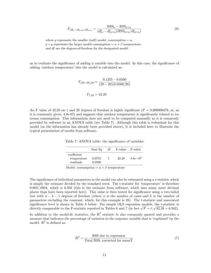
us to evaluate the significance of adding a variable into the model. In this case, the significance ofadding ‘outdoor temperature’ into the model is calculated as:

F(29−28),28 =0.1255− 0.0500

(29− 28)(0.0500/28)

F1,28 = 42.28

An F value of 42.28 on 1 and 28 degrees of freedom is highly significant (P = 0.000000479, or, asit is commonly given, 4.8e-07) and suggests that outdoor temperature is significantly related to icecream consumption. This information does not need to be computed manually as it is commonlyprovided by software in an ANOVA table (see Table 7). Although this table is redundant for thismodel (as the information has already been provided above), it is included here to illustrate thetypical presentation of results from software.

Table 7: ANOVA table: the significance of variables

Sum Sq df F-value P-value

coefficienttemperature 0.0755 1 42.28 4.8e−07residuals 0.0500

Model: consumption = α+ β temperature

The significance of individual parameters in the model can also be estimated using a t-statistic whichis simply the estimate divided by the standard error. The t-statistic for ‘temperature’ is therefore0.003/.0004, which is 6.502 (this is the estimate from software, which uses many more decimalplaces than have been reported here). This value is then tested for significance using a two-tailedtest with n − k − 1 degrees of freedom (where n is the number of cases and k is the number ofparameters excluding the constant, which, for this example is 28). The t-statistic and associatedsignificance level is shown in Table 8 below. For simple OLS regression models, the t-statistic isdirectly comparable to the F-statistic reported in Tables 6 and 7 (in fact

√F = t;

√42.28 = 6.502).

In addition to the model-fit statistics, the R2 statistic is also commonly quoted and provides ameasure that indicates the percentage of variation in the response variable that is ‘explained’ by themodel. R2 is defined as:

R2 =RSS due to regression

Total RSS, corrected for meanY(7)

11

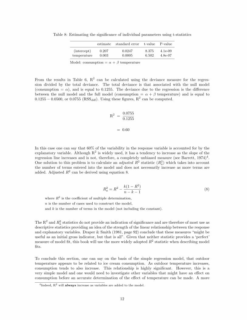
Table 8: Estimating the significance of individual parameters using t-statistics

estimate standard error t-value P-value

(intercept) 0.207 0.0247 8.375 4.1e-09temperature 0.003 0.0005 6.502 4.8e-07

Model: consumption = α + β temperature

From the results in Table 6, R2 can be calculated using the deviance measure for the regres-sion divided by the total deviance. The total deviance is that associated with the null model(consumption = α), and is equal to 0.1255. The deviance due to the regression is the differencebetween the null model and the full model (consumption = α + β temperature) and is equal to0.1255− 0.0500, or 0.0755 (RSSdiff). Using these figures, R2 can be computed.

R2 =0.0755

0.1255

= 0.60

In this case one can say that 60% of the variability in the response variable is accounted for by theexplanatory variable. Although R2 is widely used, it has a tendency to increase as the slope of theregression line increases and is not, therefore, a completely unbiased measure (see Barrett, 1974)4.One solution to this problem is to calculate an adjusted R2 statistic (R2

a) which takes into accountthe number of terms entered into the model and does not necessarily increase as more terms areadded. Adjusted R2 can be derived using equation 8.

R2a = R2 − k(1−R2)

n− k − 1(8)

where R2 is the coefficient of multiple determination,

n is the number of cases used to construct the model,

and k is the number of terms in the model (not including the constant).

The R2 and R2a statistics do not provide an indication of significance and are therefore of most use as

descriptive statistics providing an idea of the strength of the linear relationship between the responseand explanatory variables. Draper & Smith (1981, page 92) conclude that these measures “might beuseful as an initial gross indicator, but that is all”. Given that neither statistic provides a ‘perfect’measure of model fit, this book will use the more widely adopted R2 statistic when describing modelfits.

To conclude this section, one can say on the basis of the simple regression model, that outdoortemperature appears to be related to ice cream consumption. As outdoor temperature increases,consumption tends to also increase. This relationship is highly significant. However, this is avery simple model and one would need to investigate other variables that might have an effect onconsumption before an accurate determination of the effect of temperature can be made. A more

4Indeed, R2 will always increase as variables are added to the model.

12

detailed investigation into ice cream consumption is shown in Section 2.2 where a multiple OLSregression model is described.

2.2 Multiple OLS regression

OLS regression can easily be adapted to include a number of explanatory variables. For example,ice cream consumption is likely to be affected by a number of variables in addition to outdoortemperature. Table 1 shows data on two other variables that might be important in predicting icecream consumption (price and family income). Ice cream consumption may be predicted using allthree explanatory variables, a model of which is shown below.

Ice cream consumption may be predicted by outdoor temperature and price and familyincome.

2.2.1 computing and interpreting model parameters

Multiple explanatory variables are represented as a linear function in much the same way as a singlevariable. The additional variables are simply added to the model (the model is thus said to beadditive). For the example above, the model above will look like:

consumption = α + β1 outdoor temperature +

β2 price + β3 family income (9)

Ice cream consumption can be predicted, at least to some extent, by taking into account the outdoortemperature, the price of the ice cream and family income. For simplicity, only the “main effects”(i.e., the effect of each variable on its own) are included in the model described below. Any interac-tions there may be between the explanatory variables are not taken into account. Table 9 providesthe parameters for the multiple OLS regression model in Equation 9.

Table 9: Regression parameters

estimate standard error

(intercept) 0.197 0.270price −1.044 0.834family income 0.003 0.001temperature 0.003 0.000

The regression parameters for each of the explanatory variables represent the average change in icecream consumption that is expected to result from a change of one unit in that explanatory variablewhen all other variables are held constant. For example, for each unit rise in price, consumptiondecreases by an average of 1.044 pints per capita5. Similarly, for each unit increase in temperature,consumption increases by an average of 0.003 pints per capita. These partial regression coefficients

5One should be aware that a unit change in price is a very large change. For the data collected, price in fact onlyfluctuates between .260 to .292.

13

identify the effect that each explanatory variable has on consumption independent of other variablesin the model (that is, it identifies the unique contribution made by the explanatory variable indetermining consumption).

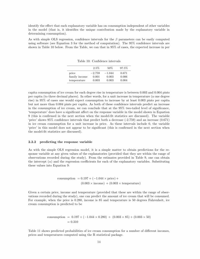
As with simple OLS regression, confidence intervals for the β parameters can be easily computedusing software (see Equation 3 for the method of computation). The 95% confidence intervals areshown in Table 10 below. From the Table, we can that in 95% of cases, the expected increase in per

Table 10: Confidence intervals

2.5% 50% 97.5%

price −2.759 −1.044 0.671family income 0.001 0.003 0.006temperature 0.003 0.003 0.004

capita consumption of ice cream for each degree rise in temperature is between 0.003 and 0.004 pintsper capita (to three decimal places). In other words, for a unit increase in temperature (a one degreerise) in 95% of cases one would expect consumption to increase by at least 0.003 pints per capitabut not more than 0.004 pints per capita. As both of these confidence intervals predict an increasein the consumption of ice cream, we can conclude that at the 95% two-tailed level of significance,‘temperature’ does have a significant affect on the response variable in the model shown in Equation9 (this is confirmed in the next section when the model-fit statistics are discussed). The variable‘price’ shows 95% confidence intervals that predict both a decrease (-2.759) and an increase (0.671)in ice cream consumption for a unit increase in price. As these intervals include 0, the variable‘price’ in this model does not appear to be significant (this is confirmed in the next section whenthe model-fit statistics are discussed).

2.2.2 predicting the response variable

As with the simple OLS regression model, it is a simple matter to obtain predictions for the re-sponse variable at any given values of the explanatories (provided that they are within the range ofobservations recorded during the study). From the estimates provided in Table 9, one can obtainthe intercept (α) and the regression coefficients for each of the explanatory variables. Substitutingthese values into Equation 9:

consumption = 0.197 + (−1.044× price) +

(0.003× income) + (0.003× temperature)

Given a certain price, income and temperature (provided that these are within the range of obser-vations recorded during the study), one can predict the amount of ice cream that will be consumed.For example, when the price is 0.280, income is 85 and temperature is 50 degrees Fahrenheit, icecream consumption is predicted to be

consumption = 0.197 + (−1.044× 0.280) + (0.003× 85) + (0.003× 50)

= 0.310

Table 11 shows predicted probabilities of ice cream consumption for a number of different incomes,prices and temperatures computed using the R statistical package.

14

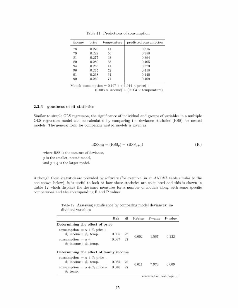
Table 11: Predictions of consumption

income price temperature predicted consumption

78 0.270 41 0.31579 0.282 56 0.35881 0.277 63 0.39480 0.280 68 0.40594 0.265 41 0.37396 0.265 52 0.41891 0.268 64 0.44090 0.260 71 0.469

Model: consumption = 0.197 + (-1.044 × price) +(0.003 × income) + (0.003 × temperature)

2.2.3 goodness of fit statistics

Similar to simple OLS regression, the significance of individual and groups of variables in a multipleOLS regression model can be calculated by comparing the deviance statistics (RSS) for nestedmodels. The general form for comparing nested models is given as:

RSSdiff = (RSSp)− (RSSp+q) (10)

where RSS is the measure of deviance,

p is the smaller, nested model,

and p+ q is the larger model.

Although these statistics are provided by software (for example, in an ANOVA table similar to theone shown below), it is useful to look at how these statistics are calculated and this is shown inTable 12 which displays the deviance measures for a number of models along with some specificcomparisons and the corresponding F and P values.

Table 12: Assessing significance by comparing model deviances: in-dividual variables

RSS df RSSdiff F-value P-value

Determining the effect of price

consumption = α+ β1 price +β2 income + β3 temp. 0.035 26

consumption = α+ 0.037 270.002 1.567 0.222

β2 income + β3 temp.

Determining the effect of family income

consumption = α+ β1 price +β2 income + β3 temp. 0.035 26

consumption = α+ β1 price + 0.046 270.011 7.973 0.009

β2 temp.

continued on next page . . .

15

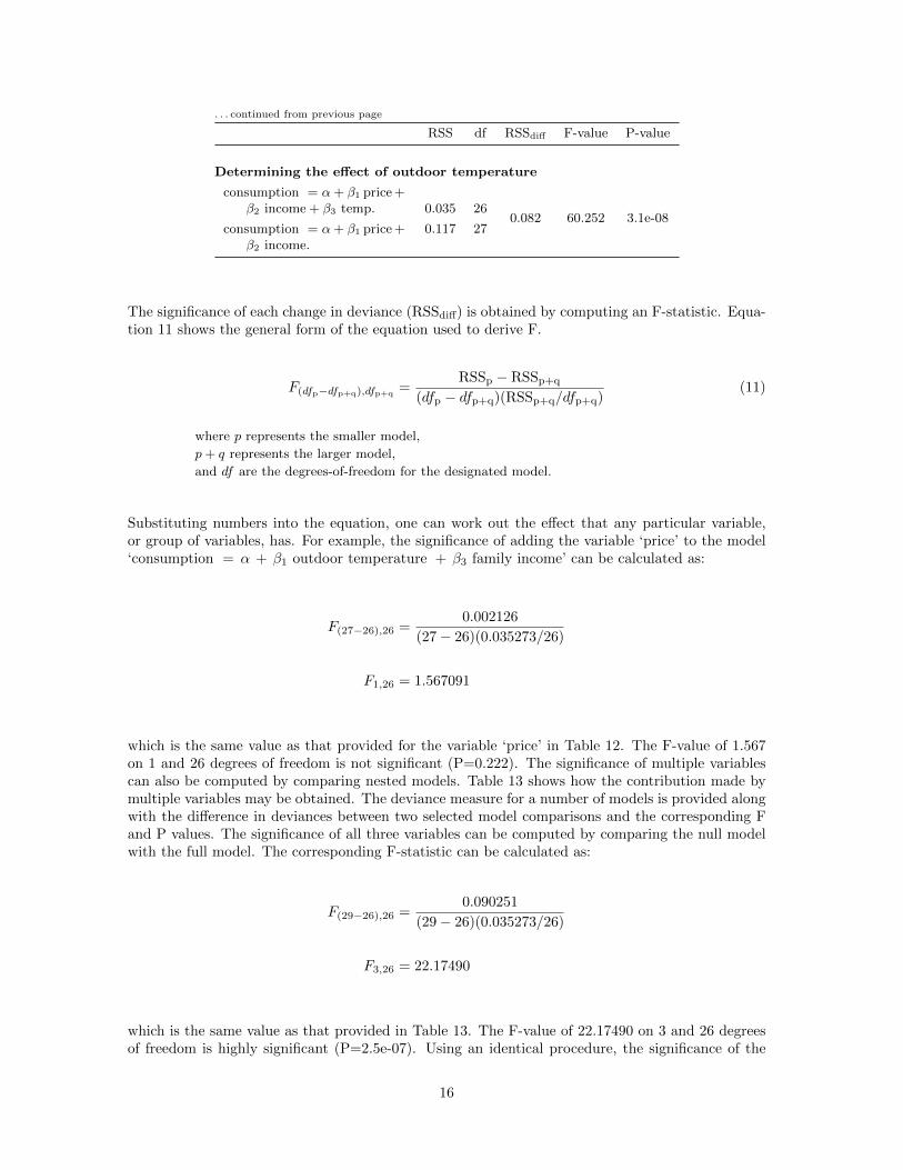
. . . continued from previous page

RSS df RSSdiff F-value P-value

Determining the effect of outdoor temperature

consumption = α+ β1 price +β2 income + β3 temp. 0.035 26

consumption = α+ β1 price + 0.117 270.082 60.252 3.1e-08

β2 income.

The significance of each change in deviance (RSSdiff) is obtained by computing an F-statistic. Equa-tion 11 shows the general form of the equation used to derive F.

F(dfp−dfp+q),dfp+q=

RSSp − RSSp+q

(dfp − dfp+q)(RSSp+q/dfp+q)(11)

where p represents the smaller model,

p+ q represents the larger model,

and df are the degrees-of-freedom for the designated model.

Substituting numbers into the equation, one can work out the effect that any particular variable,or group of variables, has. For example, the significance of adding the variable ‘price’ to the model‘consumption = α + β1 outdoor temperature + β3 family income’ can be calculated as:

F(27−26),26 =0.002126

(27− 26)(0.035273/26)

F1,26 = 1.567091

which is the same value as that provided for the variable ‘price’ in Table 12. The F-value of 1.567on 1 and 26 degrees of freedom is not significant (P=0.222). The significance of multiple variablescan also be computed by comparing nested models. Table 13 shows how the contribution made bymultiple variables may be obtained. The deviance measure for a number of models is provided alongwith the difference in deviances between two selected model comparisons and the corresponding Fand P values. The significance of all three variables can be computed by comparing the null modelwith the full model. The corresponding F-statistic can be calculated as:

F(29−26),26 =0.090251

(29− 26)(0.035273/26)

F3,26 = 22.17490

which is the same value as that provided in Table 13. The F-value of 22.17490 on 3 and 26 degreesof freedom is highly significant (P=2.5e-07). Using an identical procedure, the significance of the

16

Table 13: Assessing significance by comparing model deviances: groups of variables

model RSS df RSSdiff F-value P-value

Determining the effect of all three variablesconsumption = α+ β1 price +

β2 income + β3 temp. 0.035 26

consumption = α 0.126 290.090 22.175 2.5e-07

Determining the effect of two variables (price and temperature)consumption = α+ β1 price +

β2 income + β3 temp. 0.035 26

consumption = α + β income 0.125 280.090 33.156 7.0e-08

combined effect of price and temperature on the full model can also be derived. The change indeviance of 0.0899 is highly significant as F2,26 = 33.156, p = 7.0e− 08. The information on model-fit for individual parameters does not need to be computed manually as it is commonly provided bysoftware in an ANOVA table (see Table 14).

Table 14: ANOVA table: the significance of variables

Sum Sq df F-value P-value

coefficientincome 0.011 1 7.973 0.009price 0.002 1 1.567 0.222temperature 0.082 1 60.252 3.1e−08residuals 0.035 26

Model: consumption = α+ β1 income + β2 price +β3 temperature

The significance of individual parameters in the model can also be estimated using a t-statistic whichis simply the estimate divided by the standard error. The t-statistic for ‘temperature’ in the model‘consumption = α + β1 income + β2 price + β3 temperature’ is 0.0034584/.0004455, which is 7.762.This value is then tested for significance using a two-tailed test with n − k − 1 degrees of freedom(where n is the number of cases and k is the number of parameters excluding the constant, which,for this example is 26). The t-statistics and associated significance levels are shown in Table 15below. For single parameter variables (i.e., not categorical), the t-statistics are directly comparableto the F-statistics reported in Tables 12 and 14 (in fact

√F = t).

From the results in Tables 12 and 13, R2 can be calculated for each model by dividing the deviancemeasure for the regression by the total deviance. For the model ‘consumption = α + β1 price +β2 income’, the deviance due to the regression (the variables price and income) is the differencebetween the deviance for the null model ‘consumption = α’ (0.126; see Table 13) and the deviancefor the model ‘consumption = α + β1 price + β2 income ’ (0.117; see Table 12). The value of R2

for this model is calculated as:

17

Table 15: Estimating the significance of individual parameters using t-statistics

estimate standard error t-value P-value

(intercept) 0.197 0.270 0.730 0.472income 0.003 0.001 2.824 0.009price 1.044 0.834 -1.252 0.222

temperature 0.003 0.000 7.762 3.1e-08

Model: consumption = α+ β1 income + β2 price + β3 temperature

R2 =0.126− 0.117

0.126

= 0.071

In this case one can say that 7.1% of the variability in the response variable is accounted for bythe explanatory variables price and income. A model that includes all three explanatory variableshas an R2 value of (0.126-0.035)/0.126, which equals 0.72. We can say that altogether, the threeexplanatory variables account for about 72% of the variance in consumption. It is a simple matterto compute R2 for the other models presented in the Tables and we leave the reader to computethese by hand or by the use of statistical software.

To conclude this section, one can say that 72% of the variability in ice cream consumption isaccounted for by the three variables price, family income and temperature. From Table 15, outdoortemperature is seen to have the most significant effect on consumption (t26 = 7.762), followed byincome (t26 = 2.824) and then price (t26 = −1.252). It should be noted, however, that theserelationships are only likely to hold within the range of the collected data. Price, for example, hasa marginal effect on consumption (p > 0.01) compared to the other variables included in the model,but its effect would be likely to change markedly if it were to be increased by, say, a factor of 100.What we can conclude is that within the price range investigated in this study, fluctuations in priceonly had a marginal effect on consumption. Also, the effect of family income is significant, but onewould advise caution when interpreting this figure as, presumably, consumption would not increaseindefinitely with family income as there is likely to be an upper limit on the amount of ice cream anindividual can consume.

References

Agresti, A. (1996). An Introduction to Categorical Data Analysis. John Wiley & Sons, Inc.

Aitkin, M. A., Anderson, D. A., Francis, B. J. and Hinde, J. P. (1989). Statistical Modelling inGLIM. Oxford University Press.

Barrett, J. P. (1974). The coefficient of determination — some limitations. The American Statisti-cian, 28, 19–20.

Collett, D. (1991). Modelling Binary Data. Chapman & Hall.

18

Collett, D. (1994). Modelling survival data in medical research Chapman & Hall.

Dobson, A. J. (2001). An Introduction to Generalized Linear Models (2nd edition). Chapman andHall.

Draper, N. and Smith, H. (1981). Applied Regression Analysis. (2nd edition). John Wiley & Sons.

Draper, N. R. and Smith, H. (1998). Applied Regression Analysis. (3rd edition). John Wiley &Sons.

Fahrmeir, L. and Tutz, G. (2002). Multivariate Statistical Modelling based on Generalized LinearModels (2nd edition). Springer-Verlag.

Gill, J. (2000). Generalized Linear Models: a unified approach. Sage Publications.

Hand, D. J., Daly, F., Lunn, A. D., McConway, K. J. and Ostrowski, E. (1994). A Handbook ofSmall Data Sets. Chapman & Hall.

Hutcheson, G. D. and Sofroniou, N. (1999). The Multivariate Social Scientist: Introductory statisticsusing generalized linear models. Sage Publications.

Hutcheson, G. D. and Moutinho, L. A. (2008). Statistical Modeling for Management. Sage Publica-tions.

Koteswara, R. K. (1970). Testing for the independence of regression disturbances. Econometrica,38, 97–117.

Lindsey, J. K. (1995). Introductory Statistics: A Modelling Approach. Oxford University Press.

Lindsey, J. K. (1997). Applying Generalized Linear Models. Springer.

Lindsey, J. K. (1999). Models for Repeated Measurements (2nd edition). Oxford University Press.

McCullagh, P. and Nelder, J. A. (1989). Generalized Linear Models. (2nd edition). Chapman andHall.

McCulloch, C. E. and Searle, S. R. (2001). Generalized, Linear, and Mixed Models. John Wiley &Sons.

Nelder, J. and Wedderburn, R. W. M. (1972). Generalized linear Models. Journal of the RoyalStatistical Society, A, 135, 370–384.

Miles, J. and Shevlin, M. (2001). Applying Regression and Correlation. Sage Publications.

19