econometrics the multiple regression model: estimationdocentes.fe.unl.pt/~azevedoj/web...

MLR Model OLS Properties OLS Coefficients Unbiasedness

EconometricsThe Multiple Regression Model: Estimation

Joao Valle e Azevedo

Faculdade de EconomiaUniversidade Nova de Lisboa

Spring Semester

Joao Valle e Azevedo (FEUNL) Econometrics Lisbon, February 2011 1 / 26


OLS

Example

Now suppose:

Earningsi = β0 + β1Educationi + β2Experiencei + β3Tenurei + u

I Experience: measured as the number of years of labor marketexperience

I Tenure: years with current employerI u contains other factors affecting earnings, it should be unrelated to

the regressors

Want to interpret the coefficients as the ”ceteris paribus” effect oftheir variation on earnings



OLS

The Gauss-Markov Assumptions for Multiple Regression

Assumption MLR.1 (Linearity in Parameters)

y = β0 + β1x1 + β2x2 + ...+ βkxk + u

Assumption MLR.2 (Random Sampling)Random sample of size n,{(xi1, xi2, ..., xik ,yi ): i=1,2,...,n} satisfyingthe above equation

y = β0 + β1x1 + β2x2 + ...+ βkxk



OLS

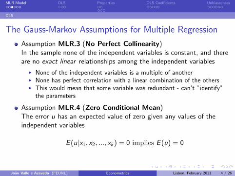
The Gauss-Markov Assumptions for Multiple Regression

Assumption MLR.3 (No Perfect Collinearity)In the sample none of the independent variables is constant, and thereare no exact linear relationships among the independent variables

I None of the independent variables is a multiple of anotherI None has perfect correlation with a linear combination of the othersI This would mean that some variable was redundant - can’t ”identify”

the parameters

Assumption MLR.4 (Zero Conditional Mean)The error u has an expected value of zero given any values of theindependent variables

E (u|x1, x2, ..., xk) = 0 implies E (u) = 0



OLS

OLS Estimatorsn∑

i=1

ui2 =

n∑i=1

(yi − β0 − β1xi1 − β2xi2 − β3xi3 − ...− βkxik)2

Let us minimize the Residuals Sum of Squares (SSR) given above.Take derivatives...

n∑i=1

(yi − β0 − β1xi1 − β2xi2 − β3xi3 − ...− βkxik) =n∑

i=1

ui = 0

n∑i=1

xi1(yi − β0 − β1xi1 − β2xi2 − β3xi3 − ...− βkxik) =n∑

i=1

xi1ui = 0

n∑i=1


i=1

xi2ui = 0

n∑i=1

xik(yi − β0 − β1xi1 − β2xi2 − β3xi3 − ...− βkxik) =n∑

i=1

xik ui = 0

We are imposing zero correlation between the regressors and theresiduals: in the population, there is also zero correlation between theerror term and the regressors...



OLS

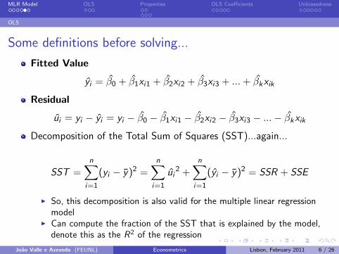
Some definitions before solving...

Fitted Value

yi = β0 + β1xi1 + β2xi2 + β3xi3 + ...+ βkxik

Residual

ui = yi − yi = yi − β0 − β1xi1 − β2xi2 − β3xi3 − ...− βkxikDecomposition of the Total Sum of Squares (SST)...again...

SST =n∑

i=1

(yi − y)2 =n∑

i=1

ui2 +

n∑i=1

(yi − y)2 = SSR + SSE

I So, this decomposition is also valid for the multiple linear regressionmodel

I Can compute the fraction of the SST that is explained by the model,denote this as the R2 of the regression



OLS

Some definitions before solving...

SST =n∑

i=1

(yi − y)2 =n∑

i=1

ui2 +

n∑i=1

(yi − y)2 = SSR + SSE

R2 =SSE

SST

= 1− SSR

SST=

[∑ni=1(yi − y)

∑ni=1(yi − ¯y)

]2

[∑ni=1(yi − y)2

][∑ni=1(yi − ¯y)2

]R2 can never decrease when another independent variable is added toa regression, and usually will increaseBecause the R2 will usually increase with the number of independentvariables, it is not a good measure to compare models



Model in Matrix Form

Solving for OLS: Model in Matrix Form

To solve for those messy first order conditions, write first the model inmatrix form

The model for the n observations of y and the regressors is:

y = Xβ + u

y=

y1

y2

...y3

, x=

1 x11 x12 ... x1k

1 x21 x22 ... x2k

... ... ... ... ...1 xn1 xn2 ... xnk

, u=

u1

u2

...un

, β=

β1

β2

...βk





Take the First Order Conditions:n∑

i=1

(yi − β0 − β1xi1 − β2xi2 − β3xi3 − ...− βkxik) =n∑

i=1

ui = 0

n∑i=1


i=1

xi1ui = 0

n∑i=1


i=1

xi2ui = 0

n∑i=1

xik(yi − β0 − β1xi1 − β2xi2 − β3xi3 − ...− βkxik) =n∑

i=1

xik ui = 0

X′u = 0⇔X′(y − Xβ) = 0

(X′X)β = X′y

β = (X′X)−1X′yJoao Valle e Azevedo (FEUNL) Econometrics Lisbon, February 2011 9 / 26




β = (X′X)−1X′y

where: y=

y1

y2

...y3

, x=

1 x11 x12 ... x1k

1 x21 x22 ... x2k

... ... ... ... ...1 xn1 xn2 ... xnk

Assumption MLR.3 (No Perfect Collinearity) implies that X has fullcolumn rank (=k+1)

This means: No column of X is a linear combination of the othercolumns

This in turn implies that (X’X)−1 exists



Unbiasedness

Properties of OLS: Unbiasedness

Theorem

Under assumptions MLR.1 to MLR.4, the OLS estimator is unbiased for β:

E(βj)=βj , j=0,1,2,...,k

Proof:

Notice that

y = Xβ + u

Then,

β = (X′X)−1X′y

= (X′X)−1X′(Xβ + u)

= (X′X)−1(X′X)β + (X′X)−1X′u

= β + (X′X)−1X′u



Unbiasedness

Properties of OLS: Unbiasedness

So, conditional on X, and using the fact that

E (u|x1, x2, ..., xk) = 0

and the fact that the sample is random, we can conclude that:

E (β) = β + (X′X)−1X′E(u|X)

= β + (X′X)−1X′0

= β



Variance

Properties of OLS: Variance

In matrix language, Var(AX)=AVar(X)A’, where X is a randomvariable

Thus,

Var(β|X ) = Var [(X′X)−1X′u|X]

= (X′X)−1X′Var(u|X)X(X′X)−1

Since X’X is symmetric (equal to its transpose) the inverse is also symmetric

= (X′X)−1X′(σ2In)X(X′X)−1

Since random sample and homoskedasticity imply Var(u|X)=σ2In

= σ2(X′X)−1X′X(X′X)−1

= σ2(X′X)−1



Variance

Properties of OLS: Estimating the Error Variance

In practice, the error variance σ2 is unknown, we must estimate it...

σ2 =

∑ni=1 ui

2

n − k − 1≡ SSR

df

I where df (degrees of freedom) is the number of observations minusthe number of estimated parameters

Can show that this is an unbiased estimator of the error variance

The standard error of the regression is given by:

σ =√σ2



Interpretation

Interpreting the Regression Coefficients

Let’s focus on the case of two explanatory variables (besides the constant),so k=2

We estimate

y = β0 + β1x1 + β2x2

It can be shown that

β1 =

∑ni=1 ri1yi∑ni=1 r

2i1

I where ri1 are the residuals obtained when we estimate the regression:

x1 = γ0 + γ2x2

Notice that β1 is the simple linear regression estimator, with ri1 instead of theoriginal regressor x1 (note that the average of the residuals is always 0)

Therefore, the estimated effect of x1 on y equals the (simple regression) estimatedeffect of the ”part” of x1 that is not explained by x2



Interpretation


Let us estimate the effect of education on wages, taking also intoaccount the effect of experience

Start by regressing education on experience (even if it seems silly...),storing the residuals of this regression

Independent Variable Coefficient Estimate Standard Error

Intercept 110.916 0.075

Labor Market Experience -0.114 0.003

n 11064

R2 0.172

Figure: Dependent Variable: Education



Interpretation


Now regress wages on the previously stored residuals


Intercept 657.893 3.524

Residual from the Education reg. 66.404 0.866

n 11064

R2 0.347

Figure: Dependent Variable: Wages



Interpretation


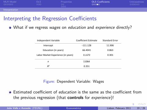
What if we regress wages on education and experience directly?


Intercept -111.128 11.906

Education (in years) 66.4041 0.863

n 11064

R2 0.351

Labor Market Experience (in years) 11.672 0.301

Figure: Dependent Variable: Wages

Estimated coefficient of education is the same as the coefficient fromthe previous regression (that controls for experience)!



Interpretation


Estimate the following regressions:

y = β0 + β1x1

y = β0 + β1x1 + β2x2

If we run regression x1 = γ0 + γ2x2 and it turns out that γ2=0, thismeans that x1 and x2 are uncorrelated.

Then the residuals from this equation are the deviations of x1 from itsmean, which implies that β1 = β1 (check the formula for β1 in thetwo interpretations)

If β2 = 0, it will also be the case that β1 = β1 (check the first orderconditions). However, in general it will be the case that β1 6= β1



Unbiasedness

Unbiasedness of OLS

Too Many or Too Few VariablesAssuming the factors in u are uncorrelated with all the consideredvariables, we have learned:

What happens if we include variables in our specification that don’tbelong?

I The estimated effects will be zero or close to zero and there is no effecton the remaining parameter estimates, and OLS remains unbiased

I Remember, if the other factors (in u) tell us nothing about theregressors (they are uncorrelated with the regressors) we can stillinterpret the estimated effects as ”ceteris paribus” effects



Unbiasedness

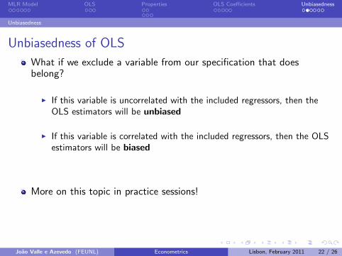
Unbiasedness of OLS

What if we exclude a variable from our specification that doesbelong?

I If this variable is uncorrelated with the included regressors, then theOLS estimators will be unbiased

I If this variable is correlated with the included regressors, then the OLSestimators will be biased

More on this topic in practice sessions!



Unbiasedness

Unbiasedness of OLS

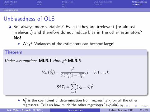
So, always more variables? Even if they are irrelevant (or almostirrelevant) and therefore do not induce bias in the other estimators?No!

I Why? Variances of the estimators can become large!

Theorem

Under assumptions MLR.1 through MLR.5

Var(βj) =σ2

SSTj(1− R2j ), j = 0, 1, ..., k

SSTj =n∑

i=1

(xij − xj)2

I R2j is the coefficient of determination from regressing xj on all the other

regressors. Tells us how much the other regressors ”explain” xjJoao Valle e Azevedo (FEUNL) Econometrics Lisbon, February 2011 23 / 26


Unbiasedness

Understanding OLS Variances

Var(βj) =σ2

SSTj(1− R2j ), j = 0, 1, ..., k

So, why can variances increase?I Strong linear relations among the independent variables are harmful: a

larger R2j implies a larger variance for the estimators (almost

multicollinearity). If we keep adding variables, R2j will always increase.

If it goes close to 1 we are in trouble...I If the new ”irrelevant” variables are uncorrelated to the already

included regressors, then the variance remains unchangedI The error variance: a larger σ2 implies a larger variance of the OLS

estimatorsI The total sample variation: a larger SSTj implies a smaller variance for

the estimators (increases with sample size, so in large samples weshould not be too worried)



Unbiasedness

Gauss-Markov Theorem

Theorem

Under assumptions MLR.1 through MLR.5 the OLS estimators areBLUE:

Best

Linear

Unbiased

Estimator

No other linear and unbiased estimator β = A′y has a smallervariance than OLS



Unbiasedness

Gauss-Markov Theorem

No other linear and unbiased estimator β = A′y has a smallervariance than OLS

Here the variances are matrices, we are saying that:

Var(β|X)− Var(β|X)

I is a positive semi-definite matrix (implies that all individual OLSparameter estimators have smaller variance than any other linearunbiased estimator for those parameters)


econometrics the multiple regression model: estimationdocentes.fe.unl.pt/~azevedoj/web...

Documents