econometrics the multiple regression model: inferencedocentes.fe.unl.pt/~azevedoj/web...
TRANSCRIPT

Normality The t Test The p-value CI The F test
EconometricsThe Multiple Regression Model: Inference
Joao Valle e Azevedo
Faculdade de EconomiaUniversidade Nova de Lisboa
Spring Semester
Joao Valle e Azevedo (FEUNL) Econometrics Lisbon, March 2011 1 / 24

Normality The t Test The p-value CI The F test
Inference
Inference in the Multiple Linear Regression Model
Suppose you want to test whether a variable is important inexplaining variation in the dependent variable:
I E.g., is the effect of tenure on wages statistically significant (ie,different from zero)? Is the effect of height on wages statisticallysignificant?
Or suppose you want to test whether a coefficient has a particularvalue
I E.g., is the effect of one additional year of schooling on expectedmonthly wages equal to 200?
Need to take into account the sampling distribution of our estimators
We will check whether under the maintained hypothesis (or nullhypothesis) the observed values of certain test statistics are likely
I If they are not we reject the null
Joao Valle e Azevedo (FEUNL) Econometrics Lisbon, March 2011 2 / 24

Normality The t Test The p-value CI The F test
Inference
Inference in the Multiple Linear Regression Model
y = β0 + β1x1 + β2x2 + ...+ βkxk + u
Assumption MLR.6 (Normality)The distribution of the population error u is independent ofx1, x2, ..., xk and u is normally distributed with mean 0 and varianceσ2: we write u ∼ Normal(0, σ2)
I Independence assumption is stronger than MLR.4 (Zero ConditionalMean) assumption. Actually, it implies MLR.4
I Also, normality and independence imply MLR.5 so that all the resultsregarding unbiasedness and variance of the estimators remain valid
Joao Valle e Azevedo (FEUNL) Econometrics Lisbon, March 2011 3 / 24
Normality The t Test The p-value CI The F test
Inference
Classical Linear Model
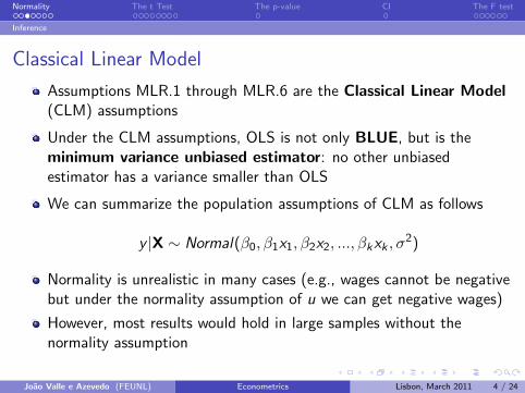
Assumptions MLR.1 through MLR.6 are the Classical Linear Model(CLM) assumptions
Under the CLM assumptions, OLS is not only BLUE, but is theminimum variance unbiased estimator: no other unbiasedestimator has a variance smaller than OLS
We can summarize the population assumptions of CLM as follows
y |X ∼ Normal(β0, β1x1, β2x2, ..., βkxk , σ2)
Normality is unrealistic in many cases (e.g., wages cannot be negativebut under the normality assumption of u we can get negative wages)
However, most results would hold in large samples without thenormality assumption
Joao Valle e Azevedo (FEUNL) Econometrics Lisbon, March 2011 4 / 24

Normality The t Test The p-value CI The F test
Inference
Normal Sampling Distribution
..
x1 x2
E(y|x) = b0 + b1x
y
f(y|x)
Normaldistributions
Figure: The homoskedastic normal distribution with a single explanatory variable
Joao Valle e Azevedo (FEUNL) Econometrics Lisbon, March 2011 5 / 24
Normality The t Test The p-value CI The F test
Inference
Normal Sampling Distribution
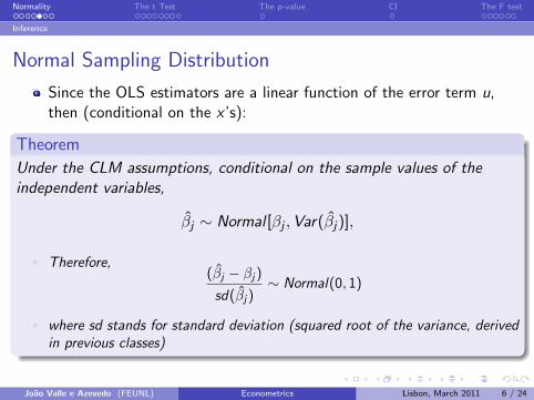
Since the OLS estimators are a linear function of the error term u,then (conditional on the x ’s):
Theorem
Under the CLM assumptions, conditional on the sample values of theindependent variables,
βj ∼ Normal [βj ,Var(βj)],
I Therefore,(βj − βj)sd(βj)
∼ Normal(0, 1)
I where sd stands for standard deviation (squared root of the variance, derivedin previous classes)
Joao Valle e Azevedo (FEUNL) Econometrics Lisbon, March 2011 6 / 24
Normality The t Test The p-value CI The F test
Inference
Normal Sampling Distribution
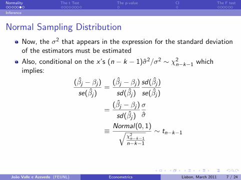
Now, the σ2 that appears in the expression for the standard deviationof the estimators must be estimated
Also, conditional on the x ’s (n − k − 1)σ2/σ2 ∼ χ2n−k−1 which
implies:
(βj − βj)se(βj)
=(βj − βj)sd(βj)
sd(βj)
se(βj)
=(βj − βj)sd(βj)
σ
σ
≡ Normal(0, 1)√χ2n−k−1
n−k−1
∼ tn−k−1
Joao Valle e Azevedo (FEUNL) Econometrics Lisbon, March 2011 7 / 24

Normality The t Test The p-value CI The F test
Inference
Normal Sampling Distribution
Theorem
Under the CLM assumptions MLR.1 through MLR.6,
(βj − βj)se(βj)
∼ tn−k−1,
where k+1 is the number of unknown parameters in the population modely = β0 + β1x1 + ...+ βkxk + u (k slope parameters and the intercept β0)
Joao Valle e Azevedo (FEUNL) Econometrics Lisbon, March 2011 8 / 24

Normality The t Test The p-value CI The F test
Inference
Performing a test on a coefficient
Set the null hypothesis (and the alternative)I E.g., H0 : βj = 0 (coefficient on experience in our wage regression) and
H1 : βj > 0
Choose a significance level (Probability of rejecting the null if the nullis actually true)
I E.g., α = 0.05
Look at the sampling distribution of the ”test statistic” t (randomvariable) involving the parameter:
t =(βj − βj)se(βj)
∼ t(n−k−1),
I Under the null hypothesis, the test statistic should be ”small” acrosssamples. Reject the null if the observed value of the test statistic isvery unlikely (very large)
Joao Valle e Azevedo (FEUNL) Econometrics Lisbon, March 2011 9 / 24
Normality The t Test The p-value CI The F test
Inference
Performing a test on a coefficient
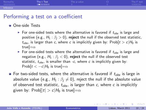
One-side Tests
I For one-sided tests where the alternative is favored if tobs is large andpositive (e.g., H1 : βj > 0), reject the null if the observed test statistic,tobs , is larger than c, where c is implicitly given by: Prob[t > c |H0 istrue]=α
I For one-sided tests where the alternative is favored if tobs is large andnegative (e.g., H1 : βj < 0), reject the null if the observed teststatistic, tobs , is smaller than -c, where c is implicitly given by:Prob[t < −c |H0 is true]=α
For two-sided tests, where the alternative is favored if tobs is large inabsolute value (e.g., H1 : βj 6= 0), reject the null if the absolute valueof observed test statistic, tobs , is larger than c, where c is implicitlygiven by: Prob[|t| > c |H0 is true]=α
Joao Valle e Azevedo (FEUNL) Econometrics Lisbon, March 2011 10 / 24
Normality The t Test The p-value CI The F test
Inference
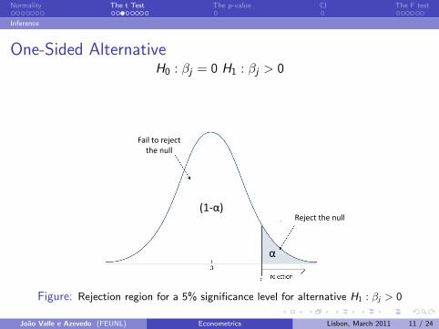
One-Sided AlternativeH0 : βj = 0 H1 : βj > 0
(1-α)
α
Reject the null
Fail to rejectthe null
Figure: Rejection region for a 5% significance level for alternative H1 : βj > 0
Joao Valle e Azevedo (FEUNL) Econometrics Lisbon, March 2011 11 / 24

Normality The t Test The p-value CI The F test
Inference
Two-Sided AlternativeH0 : βj = 0 H1 : βj 6= 0
(1-α)
α/2α/2
Reject the null
Fail to rejectthe null
Reject the null
Figure: Rejection region for a 5% significance level for alternative H1 : βj 6= 0
Joao Valle e Azevedo (FEUNL) Econometrics Lisbon, March 2011 12 / 24

Normality The t Test The p-value CI The F test
Inference
Example: Hypothesis Testing
Independent Variable Coefficient Estimate Standard Error
Intercept 5.33815 0.01218
Education (in years) 0.07614 0.00079
n 11064
R2 0.4774
Labor Market Experience (in years) 0.03093 0.00087
Square of Labor Market Experience (inyears)
-0.00038 0.000018
t ratio
438.36
96.75
35.38
-20.64
Figure: Dependent Variable: Log of Wages
The ”t ratios” are the observed values of the test statistic for testingβj = 0
I E.g. 96.75=0.07614/0.00079
Joao Valle e Azevedo (FEUNL) Econometrics Lisbon, March 2011 13 / 24
Normality The t Test The p-value CI The F test
Inference
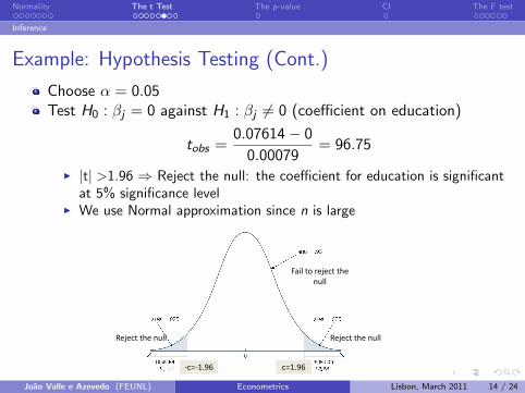
Example: Hypothesis Testing (Cont.)
Choose α = 0.05Test H0 : βj = 0 against H1 : βj 6= 0 (coefficient on education)
tobs =0.07614− 0
0.00079= 96.75
I |t| >1.96 ⇒ Reject the null: the coefficient for education is significantat 5% significance level
I We use Normal approximation since n is large
Reject the null Reject the null
Fail to reject thenull
-c=-1.96 c=1.96
Joao Valle e Azevedo (FEUNL) Econometrics Lisbon, March 2011 14 / 24
Normality The t Test The p-value CI The F test
Inference
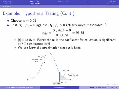
Example: Hypothesis Testing (Cont.)
Choose α = 0.05Test H0 : βj = 0 against H1 : βj > 0 (clearly more reasonable...)
tobs =0.07614− 0
0.00079= 96.75
I |t| >1.645 ⇒ Reject the null: the coefficient for education is significantat 5% significance level
I We use Normal approximation since n is large
Fail to reject thenull
Reject the null
c=1.645
Joao Valle e Azevedo (FEUNL) Econometrics Lisbon, March 2011 15 / 24
Normality The t Test The p-value CI The F test
Inference
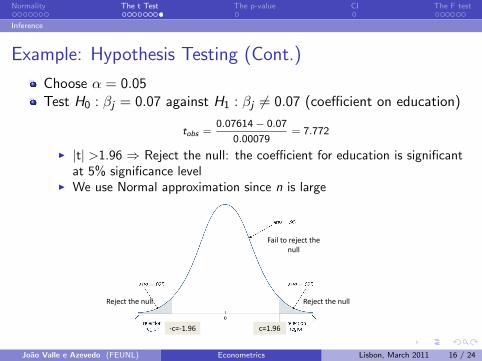
Example: Hypothesis Testing (Cont.)
Choose α = 0.05Test H0 : βj = 0.07 against H1 : βj 6= 0.07 (coefficient on education)
tobs =0.07614− 0.07
0.00079= 7.772
I |t| >1.96 ⇒ Reject the null: the coefficient for education is significantat 5% significance level
I We use Normal approximation since n is large
Reject the null Reject the null
Fail to reject thenull
-c=-1.96 c=1.96
Joao Valle e Azevedo (FEUNL) Econometrics Lisbon, March 2011 16 / 24

Normality The t Test The p-value CI The F test
Inference
p-value
p-value: Given the observed value of the t statistic, what would bethe smallest significance level at which the null H0 : βj = 0 would berejected against the alternative H1 : βj 6= 0?
I It is given by:
Prob[|t| > |tobs | | H0 true]
“p-value”/2 “p-value”/2
1-“p-value”
-tobs tobs
Figure: If the α > p − value we would reject the null!
Joao Valle e Azevedo (FEUNL) Econometrics Lisbon, March 2011 17 / 24
Normality The t Test The p-value CI The F test
Inference
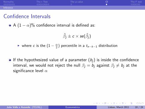
Confidence Intervals
A (1− α)% confidence interval is defined as:
βj ± c × se(βj)
I where c is the (1− α2 ) percentile in a tn−k−1 distribution
If the hypothesized value of a parameter (bj) is inside the confidenceinterval, we would not reject the null βj = bj against βj 6= bj at thesignificance level α
Joao Valle e Azevedo (FEUNL) Econometrics Lisbon, March 2011 18 / 24
Normality The t Test The p-value CI The F test
Inference
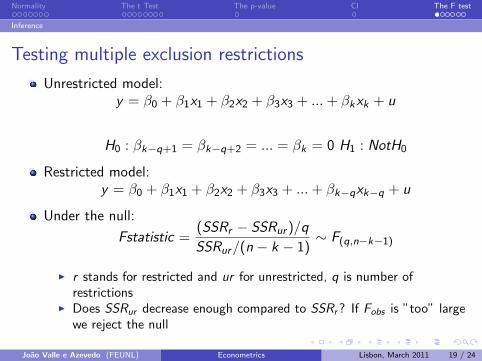
Testing multiple exclusion restrictions
Unrestricted model:y = β0 + β1x1 + β2x2 + β3x3 + ...+ βkxk + u
H0 : βk−q+1 = βk−q+2 = ... = βk = 0 H1 : NotH0
Restricted model:y = β0 + β1x1 + β2x2 + β3x3 + ...+ βk−qxk−q + u
Under the null:
Fstatistic =(SSRr − SSRur )/q
SSRur/(n − k − 1)∼ F(q,n−k−1)
I r stands for restricted and ur for unrestricted, q is number ofrestrictions
I Does SSRur decrease enough compared to SSRr? If Fobs is ”too” largewe reject the null
Joao Valle e Azevedo (FEUNL) Econometrics Lisbon, March 2011 19 / 24
Normality The t Test The p-value CI The F test
Inference
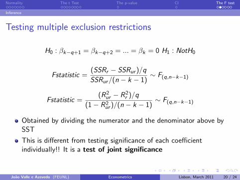
Testing multiple exclusion restrictions
H0 : βk−q+1 = βk−q+2 = ... = βk = 0 H1 : NotH0
Fstatistic =(SSRr − SSRur )/q
SSRur/(n − k − 1)∼ F(q,n−k−1)
Fstatistic =(R2
ur − R2r )/q
(1− R2ur )/(n − k − 1)
∼ F(q,n−k−1)
Obtained by dividing the numerator and the denominator above bySST
This is different from testing significance of each coefficientindividually!! It is a test of joint significance
Joao Valle e Azevedo (FEUNL) Econometrics Lisbon, March 2011 20 / 24
Normality The t Test The p-value CI The F test
Inference
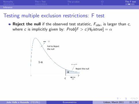
Testing multiple exclusion restrictions: F test
Reject the null if the observed test statistic, Fobs , is larger than c,where c is implicitly given by: Prob[F > c |H0istrue] = α
c
1-α
α
Fail to Rejectthe null
Reject the null
Joao Valle e Azevedo (FEUNL) Econometrics Lisbon, March 2011 21 / 24

Normality The t Test The p-value CI The F test
Inference
Example
H0 : β2 = β3 = 0
Independent Variable Coefficient Estimate Standard Error
Intercept 5.33815 0.01218
Education (in years) 0.07614 0.00079
Mean Square Error 0.11342
R2 0.4774
Labor Market Experience (in years) 0.03093 0.00087
Square of Labor Market Experience (inyears)
-0.00038 0.000018
t ratio
438.36
96.75
35.38
-20.64
Unrestricted model
Intercept 5.88400 0.00729
Education (in years) 0.06046 0.00081
Mean Square Error 0.14379
R2 0.3374
807.45
75.05
Restricted model
Figure: Dependent Variable: Log of monthly wage, n=11064
Joao Valle e Azevedo (FEUNL) Econometrics Lisbon, March 2011 22 / 24

Normality The t Test The p-value CI The F test
Inference
Example (Cont.)
α = 0.05
H0 : β2 = β3 = 0
Fstatistic =(0.4774− 0.3374)/2
(1− 0.4774)/(11064− 3− 1)
= 1581.4 > 3.00⇒ Reject H0
Joao Valle e Azevedo (FEUNL) Econometrics Lisbon, March 2011 23 / 24
Normality The t Test The p-value CI The F test
Inference
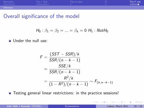
Overall significance of the model
H0 : β1 = β2 = ... = βk = 0 H1 : NotH0
Under the null use:
F =(SST − SSR)/k
SSR/(n − k − 1)
=SSE/k
SSR/(n − k − 1)
=R2/k
(1− R2)/(n − k − 1)∼ F(k,n−k−1)
Testing general linear restrictions: in the practice sessions!
Joao Valle e Azevedo (FEUNL) Econometrics Lisbon, March 2011 24 / 24