gitman 12e 525314 im ch05 - gimmenotes.co.zashift upward in an amount equal to the expected increase...

Chapter 5

Risk and return

Instructor’s resources

Overview

This chapter focuses on the fundamentals of the risk and return relationship of assets and their valuation.

For the single asset held in isolation, risk is measured with the probability distribution and its associated

statistics: the mean, the standard deviation, and the coefficient of variation. The concept of diversification

is examined by measuring the risk of a portfolio of assets that are perfectly positively correlated, perfectly

negatively correlated, and those that are uncorrelated. Next, the chapter looks at international diversification

and its effect on risk. The Capital Asset Pricing Model (CAPM) is then presented as a valuation tool for

securities and as a general explanation of the risk–return tradeoff involved in all types of financial

transactions. Chapter 5 highlights the importance of understanding the relationship of risk and return

when making professional and personal decisions.

Study Guide

The following Study Guide examples are suggested for classroom presentation:

Example Topic

4 Risk attitudes

6 Graphic determination of beta

12 Impact of market changes on return

Suggested answer to chapter opening critical thinking question

Venture capital is a form of private equity in which capital is raised in private markets as opposed

to the public markets. How can the venture capitalists eventually capitalise on their investments?

Venture capital firms investing in new and promising technologies and start-up companies must find a

buyer in order to capitalise on their investment. The ‘exit’ or ‘selling out’ is often achieved via an initial

public offering (IPO). Another option is to sell their stake in the company to another venture capital firm

or private-equity firm.

Answers to Review Questions

1. Risk is defined as the chance of financial loss, as measured by the variability of expected returns

associated with a given asset. A decision-maker should evaluate an investment by measuring the

chance of loss, or risk, and comparing the expected risk to the expected return. Some assets are

considered risk free; the most ordinary examples are RSA Treasury issues.

110 Gitman • Principles of Managerial Finance, Twelfth Edition

2. The return on an investment (total gain or loss) is the change in value plus any cash distributions over

a defined time period. It is expressed as a percent of the beginning-of-the-period investment. The

formula is:

[(ending value initial value) cash distribution]Return

initial value

Realised return requires the asset to be purchased and sold during the time periods the return is

measured. Unrealised return is the return that could have been realised if the asset had been

purchased and sold during the time period the return was measured.

3. a. The risk-averse financial manager requires an increase in return for a given increase in risk.

b. The risk-indifferent manager requires no change in return for an increase in risk.

c. The risk-seeking manager accepts a decrease in return for a given increase in risk.

Most financial managers are risk averse.

4. Scenario analysis evaluates asset risk by using more than one possible set of returns to obtain a sense

of the variability of outcomes. The range is found by subtracting the pessimistic outcome from the

optimistic outcome. The larger the range, the greater the risk associated with the asset.

5. The decision-maker can get an estimate of project risk by viewing a plot of the probability

distribution, which relates probabilities to expected returns and shows the degree of dispersion of

returns. The more spread out the distribution, the greater the variability or risk associated with the

return stream.

6. The standard deviation of a distribution of asset returns is an absolute measure of dispersion of risk

around the mean or expected value. A higher standard deviation indicates a greater project risk.

With a larger standard deviation, the distribution is more dispersed and the outcomes have a higher

variability, resulting in higher risk.

7. The coefficient of variation is another indicator of asset risk, however this measures relative

dispersion. It is calculated by dividing the standard deviation by the expected value. The coefficient

of variation may be a better basis than the standard deviation for comparing risk of assets with

differing expected returns.

8. An efficient portfolio is one that maximises return for a given risk level or minimises risk for a given

level of return. Return of a portfolio is the weighted average of returns on the individual component

assets:

1

ˆ ˆn

p j j

j

r w r

where:

n number of assets,

wj weight of individual assets,

jk expected returns.

Chapter 5 Risk and return 111

The standard deviation of a portfolio is not the weighted average of component standard deviations;

the risk of the portfolio as measured by the standard deviation will be smaller. It is calculated by

applying the standard deviation formula to the portfolio assets:

2

1

( )

( 1)

ni

rp

i

r r

n

9. The correlation between asset returns is important when evaluating the effect of a new asset on the

portfolio’s overall risk. Returns on different assets moving in the same direction are positively

correlated, while those moving in opposite directions are negatively correlated. Assets with high

positive correlation increase the variability of portfolio returns; assets with high negative correlation

reduce the variability of portfolio returns. When negatively correlated assets are brought together

through diversification, the variability of the expected return from the resulting combination can be

less than the variability or risk of the individual assets. When one asset has high returns, the other’s

returns are low and vice versa. Therefore, the result of diversification is to reduce risk by providing a

pattern of stable returns.

Diversification of risk in the asset selection process allows the investor to reduce overall risk by

combining negatively correlated assets so that the risk of the portfolio is less than the risk of the

individual assets in it. Even if assets are not negatively correlated, the lower the positive correlation

between them, the lower their resulting portfolio return variability.

10. The inclusion of foreign assets in a domestic company’s portfolio reduces risk for two reasons. When

returns from foreign-currency-denominated assets are translated into rands, the correlation of returns

of the portfolio’s assets is reduced. Also, if the foreign assets are in countries that are less sensitive to

the RSA business cycle, the portfolio’s response to market movements is reduced.

When the rand appreciates relative to other currencies, the rand value of a foreign-currency-

denominated portfolio declines and results in lower returns in rand terms. If this appreciation is due to

better performance of the RSA economy, foreign-currency-denominated portfolios generally have

lower returns in local currency as well, further contributing to reduced returns.

Political risks result from possible actions by the host government that are harmful to foreign

investors or possible political instability that could endanger foreign assets. This form of risk is

particularly high in developing countries. Companies diversifying internationally may have assets

seized or the return of profits blocked.

11. The total risk of a security is the combination of nondiversifiable risk and diversifiable risk.

Diversifiable risk refers to the portion of an asset’s risk attributable to firm-specific, random events

(strikes, litigation, loss of key contracts, etc.) that can be eliminated by diversification.

Nondiversifiable risk is attributable to market factors affecting all firms (war, inflation, political

events, etc.). Some argue that nondiversifiable risk is the only relevant risk because diversifiable risk

can be eliminated by creating a portfolio of assets that is not perfectly positively correlated.

12. Beta measures nondiversifiable risk. It is an index of the degree of movement of an asset’s return in

response to a change in the market return. The beta coefficient for an asset can be found by plotting

the asset’s historical returns relative to the returns for the market. By using statistical techniques, the

‘characteristic line’ is fit to the data points. The slope of this line is beta. Beta coefficients for

actively traded shares are published in the Value Line Investment Survey, in brokerage reports, and

several online sites. The beta of a portfolio is calculated by finding the weighted average of the betas

of the individual component assets.


13. The equation for the capital asset pricing model is:

rj RF [bj(rm RF)],

where:

rj the required (or expected) return on asset j

RF the rate of return required on a risk-free security (a U.S. Treasury bill)

bj the beta coefficient or index of nondiversifiable (relevant) risk for asset j

rm the required return on the market portfolio of assets (the market return)

The security market line (SML) is a graphical presentation of the relationship between the amount of

systematic risk associated with an asset and the required return. Systematic risk is measured by beta

and is on the horizontal axis while the required return is on the vertical axis.

14. a. If there is an increase in inflationary expectations, the security market line will show a parallel

shift upward in an amount equal to the expected increase in inflation. The required return for a

given level of risk will also rise.

b. The slope of the SML (the beta coefficient) will be less steep if investors become less risk-

averse, and a lower level of return will be required for each level of risk.

15. The CAPM provides financial managers with a link between risk and return. Because it was

developed to explain the behaviour of securities’ prices in efficient markets and uses historical data to

estimate required returns, it may not reflect future variability of returns. While studies have supported

the CAPM when applied in active securities’ markets, it has not been found to be generally applicable

to real corporate assets. However, the CAPM can be used as a conceptual framework to evaluate the

relationship between risk and return.

Suggested answer to critical thinking question for Focus on Practice

There is a difference between international mutual funds and global mutual funds. How might that

difference affect their correlation with U.S. equity mutual funds?

The difference between global funds and international funds is that global funds can invest in shares and

bonds around the world, including U.S. securities, whereas international funds invest in shares and bonds

around the world but not U.S securities. Therefore, global funds are more likely to be correlated with U.S.

equity mutual funds, since a significant portion of their portfolios are likely to be U.S. equities. An investor

seeking increased international diversification in a portfolio should consider international funds over global

funds or increase the portion of the portfolio devoted to global funds if seeking diversification through

global funds.

Suggested answer to critical thinking question for Focus on Ethics

Is ‘hitting the numbers’ an appropriate goal, given the Chapter 1 contrast of profit and shareholder

wealth maximisation? If not, why do executives emphasise it?

The presentation in Chapter 1 of our textbook is clear (and see also the moral imperative in the Chapter 1

ethics focus box): managers are to maximise shareholder wealth, not profits. Shareholder wealth

encompasses cash flow amount, timing, and risk – all of which are missed by an earnings per share (EPS)

focus. Further, to the extent that managers focus on profit, they should target long-run economic profit, not


next quarter’s EPS. Really, there are only two justifications for management attention on EPS: (1) profits

are a large and a necessary part of operating cash flows (think of the indirect approach to the statement of

cash flows, in the operating section); and (2) investors may use EPS changes to enable reevaluation of the

company’s business strategy and trend line. (In Chapter 7, you will be presented with the price-earnings

multiple approach to share valuation.)

Answers to Warm-up exercises

E5-1. Total annual return

Answer:

1 1 01

0

$0 $12,000,000 $10,000,00020%

$10,000,000

C P PK

P

Logistics, Ltd doubled the annual rate of return predicted by the analyst. The negative net

income is irrelevant to the problem.

E5-2. Expected return

Answer:

Analyst Probability Return Weighted value

1 0.35 5% 1.75%

2 0.05 5% 0.25%

3 0.20 10% 2.0%

4 0.40 3% 1.2%

Total 1.00 Expected return 4.70%

E5-3. Comparing the risk of two investments

Answer: CV1 0.10 0.15 0.6667 CV2 0.05 0.12 0.4167

Based solely on standard deviations, Investment 2 has lower risk than Investment 1. Based on

coefficients of variation, Investment 2 is still less risky than Investment 1. Since the two

investments have different expected returns, using the coefficient of variation to assess risk is

better than simply comparing standard deviations because the coefficient of variation considers

the relative size of the expected returns of each investment.

E5-4. Computing the expected return of a portfolio

Answer:

(0.45 0.038) (0.40 0.124) (0.15 0.175)

(0.0171) (0.0496) (0.02625) 0.09205 9.29%

pr

The portfolio is expected to have a return of approximately 9.3%.

E5-5. Calculating a portfolio beta

Answer:

Beta (0.20 1.15) (0.10 0.85) (0.15 1.60) (0.20 1.35) (0.35 1.85)

0.2300 0.0850 0.2400 0.2700 0.6475 1.4725


E5-6. Calculating the required rate of return

Answer:

a. Required return = 0.05 + 1.8 (0.10 0.05) = 0.05 0.09 = 0.14

b. Required return = 0.05 + 1.8 (0.13 – 0.05) = 0.05 0.144 = 0.194

c. Although the risk-free rate does not change, as the market return increases, the required

return on the asset rises by 180% of the change in the market’s return.

Solutions to Problems

P5-1. LG 1: Rate of return: 1

1( )

t

t t t

t

P P Cr =

P

Basic

a. Investment X: Return (R21,000 R20,000 R1,500)

12.50%R20,000

Investment Y: Return (R55,000 R55,000 R6,800)

12.36%R55,000

b. Investment X should be selected because it has a higher rate of return for the same level

of risk.

P5-2. LG 1: Return calculations: 1

1( )

t

t t t

t

P P Cr =

P

Basic

Investment Calculation rt(%)

A (R1,100 R800 R100) R800 25.00

B (R118,000 R120,000 R15,000)

R120,000

10.83

C (R48,000 R45,000 R7,000) R45,000 22.22

D (R500 R600 R80) R600 3.33

E (R12,400 R12,500 R1,500) R12,500 11.20

P5-3. LG 1: Risk preferences

Intermediate

a. The risk-indifferent manager would accept Investments X and Y because these have higher

returns than the 12% required return and the risk doesn’t matter.

b. The risk-averse manager would accept Investment X because it provides the highest return

and has the lowest amount of risk. Investment X offers an increase in return for taking on

more risk than what the firm currently earns.

c. The risk-seeking manager would accept Investments Y and Z because he or she is willing to

take greater risk without an increase in return.

d. Traditionally, financial managers are risk averse and would choose Investment X, since it

provides the required increase in return for an increase in risk.


P5-4. LG 2: Risk analysis

Intermediate

a.

Expansion Range

A 24% 16% 8%

B 30% 10% 20%

b. Project A is less risky, since the range of outcomes for A is smaller than the range for

Project B.

c. Since the most likely return for both projects is 20% and the initial investments are equal, the

answer depends on your risk preference.

d. The answer is no longer clear, since it now involves a risk–return tradeoff. Project B has a

slightly higher return but more risk, while A has both lower return and lower risk.

P5-5. LG 2: Risk and probability

Intermediate

a.

Camera Range

R 30% 20% 10%

S 35% 15% 20%

b

Possible

Outcomes

Probability

Pri

Expected Return

ri

Weighted

value (%)(ri Pri)

Camera R Pessimistic 0.25 20 5.00

Most likely 0.50 25 12.50

Optimistic 0.25 30 7.50

1.00 Expected return 25.00

Camera S Pessimistic 0.20 15 3.00

Most likely 0.55 25 13.75

Optimistic 0.25 35 8.75


c. Camera S is considered more risky than Camera R because it has a much broader range of

outcomes. The risk–return tradeoff is present because Camera S is more risky and also

provides a higher return than Camera R.


P5-6. LG 2: Bar charts and risk

Intermediate

a.


b.

Market

acceptance

Probability

Pri

Expected return

ri

Weighted value

(ri Pri)

Line J Very poor 0.05 0.0075 0.000375

Poor 0.15 0.0125 0.001875

Average 0.60 0.0850 0.051000

Good 0.15 0.1475 0.022125

Excellent 0.05 0.1625 0.008125


Line K Very poor 0.05 0.010 0.000500

Poor 0.15 0.025 0.003750

Average 0.60 0.080 0.048000

Good 0.15 0.135 0.020250

Excellent 0.05 0.150 0.007500


c. Line K appears less risky due to a slightly tighter distribution than line J, indicating a lower

range of outcomes.

P5-7. LG 2: Coefficient of variation: rCVr

Basic

a. A 7%

0.350020%

ACV

B 9.5%

0.431822%

BCV

C 6%

0.315819%

CCV

D 5.5%

0.343816%

DCV

b. Asset C has the lowest coefficient of variation and is the least risky relative to the other choices.

P5-8. LG 2: Standard deviation versus coefficient of variation as measures of risk

Basic

a. Project A is least risky based on range with a value of 0.04.

b. Project A is least risky based on standard deviation with a value of 0.029. Standard deviation

is not the appropriate measure of risk since the projects have different returns.


c. A 0.029

0.24170.12

ACV

B 0.032

0.25600.125

BCV

C 0.035

0.26920.13

CCV

D 0.030

0.23440.128

DCV

In this case Project D is the best alternative since it provides the least amount of risk for each

percent of return earned. Coefficient of variation is probably the best measure in this instance

since it provides a standardised method of measuring the risk–return tradeoff for investments

with differing returns.

P5-9. LG 2: Personal finance: Rate of return, standard deviation, coefficient of variation

Challenge

a. Share price Variance

Year Beginning End Returns (Return–Average Return)2

2006

2007

2008

2009

14.36

21.55

64.78

72.38

21.55

64.78

72.38

91.80

50.07%

200.60%

11.73%

26.83%

0.0495

1.6459

0.3670

0.2068

b. Average return 72.31%

c. Sum of variances 2.2692

3 Sample divisor (n 1)

0.7564 Variance

86.97% Standard deviation

d. 1.20 Coefficient of variation

e. The share price of Idion has definitely gone through some major price changes over this

time period. It would have to be classified as a volatile security having an upward price

trend over the past four years. Note how comparing securities on a CV basis allows the

investor to put the share in proper perspective. The share is riskier than what Mike normally

buys but if he believes that Idion will continue to rise then he should include it.


P5-10. LG 2: Assessing return and risk

Challenge

a. Project 257

(1) Range: 1.00 (.10) 1.10

(2) Expected return: =1

n

i ri

i

r r P

Rate of return

ri

Probability

Pr i

Weighted value

ri Pr i

Expected return

1

n

i ri

i

r r P

.10 0.01 0.001

0.10 0.04 0.004

0.20 0.05 0.010

0.30 0.10 0.030

0.40 0.15 0.060

0.45 0.30 0.135

0.50 0.15 0.075

0.60 0.10 0.060

0.70 0.05 0.035

0.80 0.04 0.032

1.00 0.01 0.010

1.00 0.450

(3) Standard deviation: 2

1

( )n

i ri

i

r r P

ri r ir r ( )

ir r

2 Pr i ( )

ir r

2Pr i

0.10 0.450 0.550 0.3025 0.01 0.003025

0.10 0.450 0.350 0.1225 0.04 0.004900

0.20 0.450 0.250 0.0625 0.05 0.003125

0.30 0.450 0.150 0.0225 0.10 0.002250

0.40 0.450 0.050 0.0025 0.15 0.000375

0.45 0.450 0.000 0.0000 0.30 0.000000

0.50 0.450 0.050 0.0025 0.15 0.000375

0.60 0.450 0.150 0.0225 0.10 0.002250

0.70 0.450 0.250 0.0625 0.05 0.003125

0.80 0.450 0.350 0.1225 0.04 0.004900

1.00 0.450 0.550 0.3025 0.01 0.003025

0.027350

Project 2570.027350 0.165378


(4) 0.165378

0.36750.450

CV

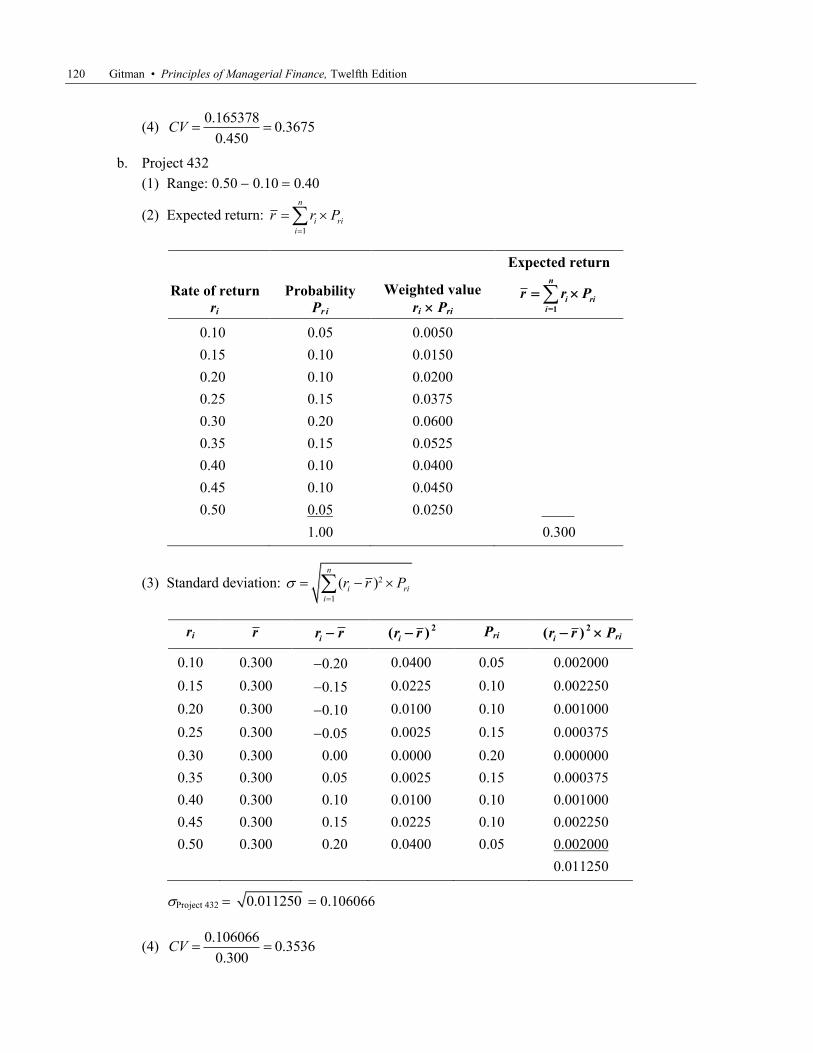
b. Project 432

(1) Range: 0.50 0.10 0.40

(2) Expected return: 1

n

i ri

i

r r P

Rate of return

ri

Probability

Pr i

Weighted value

ri Pri

Expected return

=1

n

i ri

i

r r P

0.10 0.05 0.0050

0.15 0.10 0.0150

0.20 0.10 0.0200

0.25 0.15 0.0375

0.30 0.20 0.0600

0.35 0.15 0.0525

0.40 0.10 0.0400

0.45 0.10 0.0450

0.50 0.05 0.0250

1.00 0.300

(3) Standard deviation: 2

1

( )n

i ri

i

r r P

ri r ir r ( )

ir r

2 Pri ( )

ir r

2Pri

0.10 0.300 0.20 0.0400 0.05 0.002000

0.15 0.300 0.15 0.0225 0.10 0.002250

0.20 0.300 0.10 0.0100 0.10 0.001000

0.25 0.300 0.05 0.0025 0.15 0.000375

0.30 0.300 0.00 0.0000 0.20 0.000000

0.35 0.300 0.05 0.0025 0.15 0.000375

0.40 0.300 0.10 0.0100 0.10 0.001000

0.45 0.300 0.15 0.0225 0.10 0.002250

0.50 0.300 0.20 0.0400 0.05 0.002000

0.011250

Project 432 0.011250 0.106066

(4) 0.106066

0.35360.300

CV


c. Bar Charts

d. Summary statistics

Project 257 Project 432

Range 1.100 0.400

Expected return ( )r 0.450 0.300

Standard deviation ( )r

0.165 0.106

Coefficient of variation (CV) 0.3675 0.3536

Since Projects 257 and 432 have differing expected values, the coefficient of variation should

be the criterion by which the risk of the asset is judged. Since Project 432 has a smaller CV, it

is the opportunity with lower risk.


P5-11. LG 2: Integrative – expected return, standard deviation, and coefficient of variation

Challenge

a. Expected return: 1

n

i ri

i

r r P

Rate of return

ri

Probability

Pr i

Weighted value

ri Pri

Expected return

1

n

i ri

i

r r P

Asset F 0.40 0.10 0.04

0.10 0.20 0.02

0.00 0.40 0.00

0.05 0.20 0.01

0.10 0.10 0.01

0.04

Asset G 0.35 0.40 0.14

0.10 0.30 0.03

0.20 0.30 0.06

0.11

Asset H 0.40 0.10 0.04

0.20 0.20 0.04

0.10 0.40 0.04

0.00 0.20 0.00

0.20 0.10 0.02

0.10

Asset G provides the largest expected return.


b. Standard deviation: 2

1

( )n

i ri

i

r r xP

ir r ( )

ir r

2 Pr i 2

r

Asset F 0.40 0.04 0.36 0.1296 0.10 0.01296

0.10 0.04 0.06 0.0036 0.20 0.00072

0.00 0.04 0.04 0.0016 0.40 0.00064

0.05 0.04 0.09 0.0081 0.20 0.00162

0.10 0.04 0.14 0.0196 0.10 0.00196

0.01790 0.1338

Asset G 0.35 0.11 .24 0.0576 0.40 0.02304

0.10 0.11 0.01 0.0001 0.30 0.00003

0.20 0.11 0.31 0.0961 0.30 0.02883

0.05190 0.2278

Asset H 0.40 0.10 .30 0.0900 0.10 0.009

0.20 0.10 .10 0.0100 0.20 0.002

0.10 0.10 0.00 0.0000 0.40 0.000

0.00 0.10 0.10 0.0100 0.20 0.002

0.20 0.10 0.30 0.0900 0.10 0.009

0.022 0.1483

Based on standard deviation, Asset G appears to have the greatest risk, but it must be

measured against its expected return with the statistical measure coefficient of variation, since

the three assets have differing expected values. An incorrect conclusion about the risk of the

assets could be drawn using only the standard deviation.

c. standard deviation ( )

Coefficient of variation =expected value

Asset F: 0.1338

3.3450.04

CV

Asset G: 0.2278

2.0710.11

CV

Asset H: 0.1483

1.4830.10

CV

As measured by the coefficient of variation, Asset F has the largest relative risk.


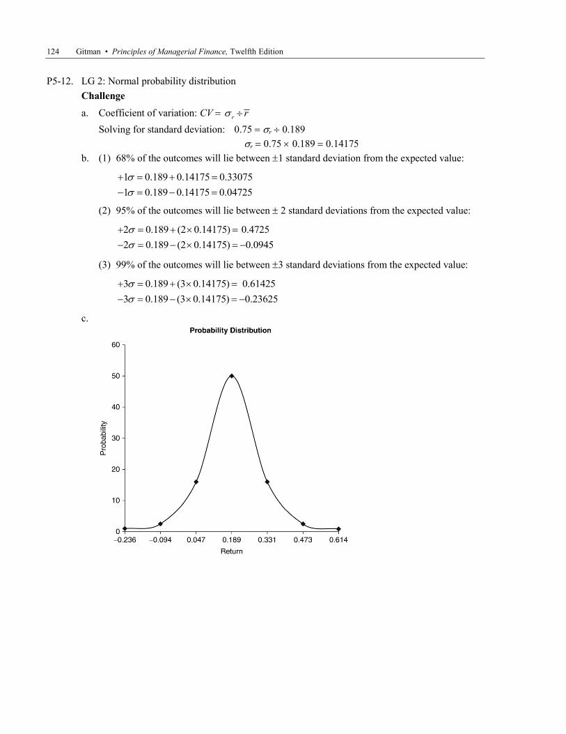
P5-12. LG 2: Normal probability distribution

Challenge

a. Coefficient of variation: CV rr

Solving for standard deviation: 0.75 r 0.189

r 0.750.189 0.14175

b. (1) 68% of the outcomes will lie between 1 standard deviation from the expected value:

1 0.189 0.14175 0.33075

1 0.189 0.14175 0.04725

(2) 95% of the outcomes will lie between 2 standard deviations from the expected value:

2 0.189 (2 0.14175) 0.4725

2 0.189 (2 0.14175) 0.0945

(3) 99% of the outcomes will lie between 3 standard deviations from the expected value:

3 0.189 (3 0.14175) 0.61425

3 0.189 (3 0.14175) 0.23625

c.


P5-13. LG 3: Personal finance: Portfolio return and standard deviation

Challenge

a. Expected portfolio return for each year: rp (wLrL) (wMrM)

Year

Asset L

(wLrL)

Asset M

(wMrM)

Expected

portfolio return

rp

2010 (14% 0.40 5.6%) (20%0.60 12.0%) 17.6%

2011 (14% 0.40 5.6%) (18%0.60 10.8%) 16.4%

2012 (16% 0.40 6.4%) (16%0.60 9.6%) 16.0%

2013 (17% 0.40 6.8%) (14%0.60 8.4%) 15.2%

2014 (17% 0.40 6.8%) (12%0.60 7.2%) 14.0%

2015 (19% 0.40 7.6%) (10%0.60 6.0%) 13.6%

b. Portfolio return: 1

n

j j

j

p

w r

rn

17.6 16.4 16.0 15.2 14.0 13.6

15.467 15.5%6

pr

c. Standard deviation:

2

1

( )

( 1)

ni

rp

i

r r

n

2 2 2

2 2 2

(17.6% 15.5%) (16.4% 15.5%) (16.0% 15.5%)

(15.2% 15.5%) (14.0% 15.5%) (13.6% 15.5%)

6 1rp

2 2 2

2 2 2

(2.1%) (0.9%) (0.5%)

( 0.3%) ( 1.5%) ( 1.9%)

5rp

(.000441 0.000081 0.000025 0.000009 0.000225 0.000361)

5rp

0.001142

0.000228% 0.0151 1.51%5

rp

d. The assets are negatively correlated.

e. Combining these two negatively correlated assets reduces overall portfolio risk.


P5-14. LG 3: Portfolio analysis

Challenge

a. Expected portfolio return:

Alternative 1: 100% Asset F

16% 17% 18% 19%17.5%

4

pr

Alternative 2: 50% Asset F 50% Asset G

Year Asset F

(wFrF)

Asset G

(wGrG)

Portfolio return

rp

2010 (16%0.50 8.0%) (17%0.50 8.5%) 16.5%

2011 (17%0.50 8.5%) (16%0.50 8.0%) 16.5%

2012 (18%0.50 9.0%) (15%0.50 7.5%) 16.5%

2013 (19%0.50 9.5%) (14%0.50 7.0%) 16.5%

16.5% 16.5% 16.5% 16.5%16.5%

4pr

Alternative 3: 50% Asset F 50% Asset H

Year Asset F

(wFrF)

Asset H

(wHrH)

Portfolio return

rp

2010 (16%0.50 8.0%) (14%0.50 7.0%) 15.0%

2011 (17%0.50 8.5%) (15%0.50 7.5%) 16.0%

2012 (18%0.50 9.0%) (16%0.50 8.0%) 17.0%

2013 (19%0.50 9.5%) (17%0.50 8.5%) 18.0%

15.0% 16.0% 17.0% 18.0%16.5%

4pr

b. Standard deviation:

2

1

( )

( 1)

ni

rp

i

r r

n

(1)

2 2 2 2[(16.0% 17.5%) (17.0% 17.5%) (18.0% 17.5%) (19.0% 17.5%) ]

4 1F

2 2 2 2[( 1.5%) ( 0.5%) (0.5%) (1.5%) ]

3

F

(0.000225 0.000025 0.000025 0.000225)

3

F

0.0005

.000167 0.01291 1.291%3

F


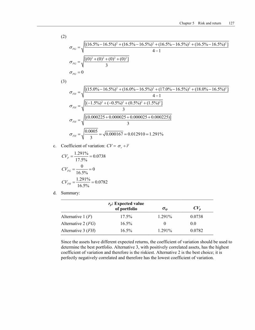
(2)

2 2 2 2[(16.5% 16.5%) (16.5% 16.5%) (16.5% 16.5%) (16.5% 16.5%) ]

4 1FG

2 2 2 2[(0) (0) (0) (0) ]

3

FG

0FG

(3)

2 2 2 2[(15.0% 16.5%) (16.0% 16.5%) (17.0% 16.5%) (18.0% 16.5%) ]

4 1FH

2 2 2 2[( 1.5%) ( 0.5%) (0.5%) (1.5%) ]

3

FH

[(0.000225 0.000025 0.000025 0.000225)]

3

FH

0.0005

0.000167 0.012910 1.291%3

FH

c. Coefficient of variation: CV rr

1.291%0.0738

17.5%F

CV

00

16.5%FG

CV

1.291%0.0782

16.5%FH

CV

d. Summary:

rp: Expected value

of portfolio rp CVp

Alternative 1 (F) 17.5% 1.291% 0.0738

Alternative 2 (FG) 16.5% 0 0.0

Alternative 3 (FH) 16.5% 1.291% 0.0782

Since the assets have different expected returns, the coefficient of variation should be used to

determine the best portfolio. Alternative 3, with positively correlated assets, has the highest

coefficient of variation and therefore is the riskiest. Alternative 2 is the best choice; it is

perfectly negatively correlated and therefore has the lowest coefficient of variation.


P5-15. LG 4: Correlation, risk, and return

Intermediate

a. (1) Range of expected return: between 8% and 13%

(2) Range of the risk: between 5% and 10%

b. (1) Range of expected return: between 8% and 13%

(2) Range of the risk: 0 risk 10%

c. (1) Range of expected return: between 8% and 13%

(2) Range of the risk: 0 risk 10%

P5-16. LG 1, 4: Personal finance: International investment returns

Intermediate

a) Pt(1000 x 24.75) 24,750 – Pt-1(1000 x 20.50)20,500/20,500 = 20,73%

b) Pt = 24,750 Mt / 2.85 = R8,684

Pt-1 = 20,500 Mt / 2.40 = R8,542

c) R8,684 – R8,542/R8,542 = 1,66%

d. The two returns differ due to the change in the exchange rate between the metical and the

rand. The metical had depreciation (and thus the rand appreciated) between the purchase date

and the sale date, causing a decrease in total return. The answer in part (c) is the more

important of the two returns for Themba. An investor in foreign securities will carry

exchange-rate risk.

P5-17. LG 5: Total, nondiversifiable, and diversifiable risk

Intermediate

a and b


c. Only nondiversifiable risk is relevant because, as shown by the graph, diversifiable risk can

be virtually eliminated through holding a portfolio of at least 20 securities that are not positively

correlated. David Randall’s portfolio, assuming diversifiable risk could no longer be reduced

by additions to the portfolio, has 6.47% relevant risk.

P5-18. LG 5: Graphic derivation of beta

Intermediate

a.

b. To estimate beta, the ‘rise over run’ method can be used: Rise

BetaRun

Y

X

Taking the points shown on the graph:

12 9 3Beta A 0.75

8 4 4

Y

X

26 22 4Beta B 1.33

13 10 3

Y

X

A financial calculator with statistical functions can be used to perform linear regression

analysis. The beta (slope) of line A is 0.79; of line B, 1.379.

c. With a higher beta of 1.33, Asset B is more risky. Its return will move 1.33 times for each one

point the market moves. Asset A’s return will move at a lower rate, as indicated by its beta

coefficient of 0.75.

P5-19. LG 5: Interpreting beta

Basic

Effect of change in market return on asset with beta of 1.20:

a. 1.20 (15%) 18.0% increase

b. 1.20 (8%) 9.6% decrease

c. 1.20 (0%) no change

d. The asset is more risky than the market portfolio, which has a beta of 1. The higher beta

makes the return move more than the market.


P5-20. LG 5: Betas

Basic

a and b

Asset

Beta

Increase in

market return

Expected impact

on asset return

Decrease in

market return

Impact on

asset return

A 0.50 0.10 0.05 0.10 0.05

B 1.60 0.10 0.16 0.10 0.16

C 0.20 0.10 0.02 0.10 0.02

D 0.90 0.10 0.09 0.10 0.09

c. Asset B should be chosen because it will have the highest increase in return.

d. Asset C would be the appropriate choice because it is a defensive asset, moving in opposition

to the market. In an economic downturn, Asset C’s return is increasing.

P5-21. LG 5: Personal finance: Betas and risk rankings

Intermediate

a.

Share Beta

Most risky B 1.40

A 0.80

Least risky C 0.30

b and c

Asset

Beta Increase in

market return

Expected impact

on asset return

Decrease in

market return

Impact on

asset return

A 0.80 0.12 0.096 0.05 0.04

B 1.40 0.12 0.168 0.05 0.07

C 0.30 0.12 0.036 0.05 0.015

d. In a declining market, an investor would choose the defensive share, Share C. While the

market declines, the return on C increases.

e. In a rising market, an investor would choose Share B, the aggressive share. As the market

rises one point, Share B rises 1.40 points.


P5-22. LG 5: Portfolio betas: bp 1

n

j j

j

w b

Intermediate

a.

Portfolio A Portfolio B

Asset Beta wA wAbA wB wBbB

1 1.30 0.10 0.130 0.30 0.39

2 0.70 0.30 0.210 0.10 0.07

3 1.25 0.10 0.125 0.20 0.25

4 1.10 0.10 0.110 0.20 0.22

5 0.90 0.40 0.360 0.20 0.18

bA 0.935 bB 1.11

b. Portfolio A is slightly less risky than the market (average risk), while Portfolio B is more

risky than the market. Portfolio B’s return will move more than Portfolio A’s for a given

increase or decrease in market return. Portfolio B is the more risky.

P5-23. LG 6: Capital asset pricing model (CAPM): rj RF [bj(rm RF)]

Basic

Case rj RF [bj(rm RF)]

A 8.9% 5% [1.30(8% 5%)]

B 12.5% 8% [0.90(13% 8%)]

C 8.4% 9% [0.20(12% 9%)]

D 15.0% 10% [1.00(15% 10%)]

E 8.4% 6% [0.60(10% 6%)]

P5-24. LG 5, 6: Personal finance: Beta coefficients and the capital asset pricing model

Intermediate

To solve this problem you must take the CAPM and solve for beta. The resulting model is:

Beta F

m F

r R

r R

a. 10% 5% 5%

Beta 0.454516% 5% 11%

b. 15% 5% 10%

Beta 0.909116% 5% 11%

c. 18% 5% 13%

Beta 1.181816% 5% 11%

d. 20% 5% 15%

Beta 1.363616% 5% 11%

e. If Katherine is willing to take a maximum of average risk then she will be able to have an

expected return of only 16%. (r 5% 1.0(16% 5%) 16%.)


P5-25. LG 6: Manipulating CAPM: rj RF [bj(rm RF)]

Intermediate

a. rj 8% [0.90(12% 8%)]

rj 11.6%

b. 15% RF [1.25(14% RF)]

RF 10%

c. 16% 9% [1.10(rm 9%)]

rm 15.36%

d. 15% 10% [bj(12.5% 10%)

bj 2

P5-26. LG 1, 3, 5, 6: Personal finance: Portfolio return and beta

Challenge

a. bp (0.20)(0.80) (0.35)(0.95) (0.30)(1.50) (0.15)(1.25)

0.16 0.3325 0.45 0.1875 1.13

b. rA (R20,000 R20,000) R1,600 R1,600

8%R20,000 R20,000

rB (R36,000 R35,000) R1,400 R2,400

6.86%R35,000 R35,000

rC (R34,500 R30,000) 0 R4,500

15%R30,000 R30,000

rD (R16,500 R15,000) R375 R1,875

12.5%R15,000 R15,000

c. rP (R107,000 R100,000) R3,375 R10,375

10.375%R100,000 R100,000

d. rA 4% [0.80(10% 4%)] 8.8%

rB 4% [0.95(10% 4%)] 9.7%

rC 4% [1.50(10% 4%)] 13.0%

rD 4% [1.25(10% 4%)] 11.5%

e. Of the four investments, only C (15% versus 13%) and D (12.5% versus 11.5%) had actual

returns that exceeded the CAPM expected return (15% versus 13%). The underperformance

could be due to any unsystematic factor that would have caused the firm not to do as well as

expected. Another possibility is that the firm’s characteristics may have changed such that the

beta at the time of the purchase overstated the true value of beta that existed during that year.

A third explanation is that beta, as a single measure, may not capture all of the systematic

factors that cause the expected return. In other words, there is error in the beta estimate.


P5-27. LG 6: Security market line, SML

Intermediate

a, b, and d

c. rj RF [bj(rm RF)]

Asset A

rj 0.09 [0.80(0.13 0.09)]

rj 0.122

Asset B

rj 0.09 [1.30(0.13 0.09)]

rj 0.142

d. Asset A has a smaller required return than Asset B because it is less risky, based on the beta

of 0.80 for Asset A versus 1.30 for Asset B. The market risk premium for Asset A is 3.2%

(12.2% 9%), which is lower than Asset B’s market risk premium (14.2% 9% 5.2%).

P5-28. LG 6: Shifts in the security market line

Challenge

a, b, c, d


b. rj RF [bj(rm RF)]

rA 8% [1.1(12% 8%)]

rA 8% 4.4%

rA 12.4%

c. rA 6% [1.1(10% 6%)]

rA 6% 4.4%

rA 10.4%

d. rA 8% [1.1(13% 8%)]

rA 8% 5.5%

rA 13.5%

e. (1) A decrease in inflationary expectations reduces the required return as shown in the

parallel downward shift of the SML.

(2) Increased risk aversion results in a steeper slope, since a higher return would be required

for each level of risk as measured by beta.

P5-29. LG 6: Integrative-risk, return, and CAPM

Challenge

a.

Project rj RF [bj(rm RF)]

A rj 9% [1.5(14% 9%)] 16.5%

B rj 9% [0.75(14% 9%)] 12.75%

C rj 9% [2.0(14% 9%)] 19.0%

D rj 9% [0(14% 9%)] 9.0%

E rj 9% [(0.5)(14% 9%)] 6.5%

b and d


c. Project A is 150% as responsive as the market.

Project B is 75% as responsive as the market.

Project C is twice as responsive as the market.

Project D is unaffected by market movement.

Project E is only half as responsive as the market, but moves in the opposite direction as the

market.

d. See graph for new SML.

rA 9% [1.5(12% 9%)] 13.50%

rB 9% [0.75(12% 9%)] 11.25%

rC 9% [2.0(12% 9%)] 15.00%

rD 9% [0(12% 9%)] 9.00%

rE 9% [0.5(12% 9%)] 7.50%

e. The steeper slope of SMLb indicates a higher risk premium than SMLd for these market

conditions. When investor risk aversion declines, investors require lower returns for any given

risk level (beta).

P5-30. Ethics problem

Intermediate

One way is to ask how the candidate would handle a hypothetical situation. One may gain insight

into the moral/ethical framework within which decisions are made. Another approach is to use a

pencil-and-paper honesty test – these are surprisingly accurate, despite the obvious notion that the

job candidate may attempt to game the exam by giving the ‘right’ versus the individually accurate

responses. Before even administering the situational interview question or the test, ask the candidate

to list the preference attributes of the type of company he or she aspires to work for, and see if

character and ethics terms emerge in the description. Some companies do credit history checks, after

gaining the candidates approval to do so. Using all four of these techniques allows one to ‘triangulate’

toward a valid and defensible appraisal of a candidate’s honesty and integrity.

Case

Analysing risk and return on Chargers Products’ investments

This case requires students to review and apply the concept of the risk–return tradeoff by analysing two

possible asset investments using standard deviation, coefficient of variation, and CAPM.

1. Expected rate of return: 1

1

( )t t t

t

t

P P Cr

P

Asset X:

Year

Cash

flow (Ct)

Ending

value (Pt)

Beginning

value (Pt – 1)

Gain/

Loss

Annual rate

of return

2000 R1,000 R22,000 R20,000 R2,000 15.00%

2001 1,500 21,000 22,000 1,000 2.27

2002 1,400 24,000 21,000 3,000 20.95

2003 1,700 22,000 24,000 2,000 1.25


Asset X: (continued)

Year

Cash

flow (Ct)

Ending

value (Pt)

Beginning

value (Pt – 1)

Gain/

Loss

Annual rate

of return

2004 1,900 23,000 22,000 1,000 13.18

2005 1,600 26,000 23,000 3,000 20.00

2006 1,700 25,000 26,000 1,000 2.69

2007 2,000 24,000 25,000 1,000 4.00

2008 2,100 27,000 24,000 3,000 21.25

2009 2,200 30,000 27,000 3,000 19.26

Average expected return for AssetX 11.74%

Asset Y:

Year

Cash

flow (Ct)

Ending

value (Pt)

Beginning

value (Pt – 1)

Gain/

Loss

Annual rate

of return

2000 R1,50

0

R20,00

0

R20,000 R 0 7.50%

2001 1,600 20,000 20,000 0 8.00

2002 1,700 21,000 20,000 1,000 13.50

2003 1,800 21,000 21,000 0 8.57

2004 1,900 22,000 21,000 1,000 13.81

2005 2,000 23,000 22,000 1,000 13.64

2006 2,100 23,000 23,000 0 9.13

2007 2,200 24,000 23,000 1,000 13.91

2008 2,300 25,000 24,000 1,000 13.75

2009 2,400 25,000 25,000 0 9.60

Average expected return for Asset Y 11.14%

2. r 2

1

( ) ( 1)n

i

i

r r n

Asset X:

Year

Return

ri Average

return, r

( )ir r

( )ir r 2

2000 15.00% 11.74% 3.26% 0.001063

2001 2.27 11.74 9.47 0.008968

2002 20.95 11.74 9.21 0.008482

2003 1.25 11.74 12.99 0.016874

2004 13.18 11.74 1.44 0.000207

2005 20.00 11.74 8.26 0.006823


Asset X: (continued)

Year

Return

ri Average

return, r

( )ir r

( )ir r

2

2006 2.69 11.74 9.05 0.008190

2007 4.00 11.74 7.74 0.005991

2008 21.25 11.74 9.51 0.009044

2009 19.26 11.74 7.52 0.005655

0.071297

0.0712970.07922 .0890 8.90%

10 1x

8.90%0.76

11.74%CV

Asset Y:

Year Return

ri

Average

return, r

( )ir r

( )ir r 2

2000 7.50% 11.14% 3.64% 0.001325

2001 8.00 11.14 3.14 0.000986

2002 13.50 11.14 2.36 0.000557

2003 8.57 11.14 2.57 0.000660

2004 13.81 11.14 2.67 0.000713

2005 13.64 11.14 2.50 0.000625

2006 9.13 11.14 2.01 0.000404

2007 13.91 11.14 2.77 0.000767

2008 13.75 11.14 2.61 0.000681

2009 9.60 11.14 1.54 0.000237

0.006955

0.0069550.0773 0.0278 2.78%

10 1

Y

2.78%0.25

11.14%CV


3. Summary statistics:

Asset X Asset Y

Expected return 11.74% 11.14%

Standard deviation 8.90% 2.78%

Coefficient of variation 0.76 0.25

Comparing the expected returns calculated in part (a), Asset X provides a return of 11.74%, only

slightly above the return of 11.14% expected from Asset Y. The higher standard deviation and

coefficient of variation of Investment X indicates greater risk. With just this information, it is

difficult to determine whether the 0.60% difference in return is adequate compensation for the

difference in risk. Based on this information, however, Asset Y appears to be the better choice.

4. Using the capital asset pricing model, the required return on each asset is as follows:

Capital asset pricing model: rj RF [bj(rm RF)]

Asset RF [bj(rm RF)] rj

X 7% [1.6(10% 7%)] 11.8%

Y 7% [1.1(10% 7%)] 10.3%

From the calculations in part (a), the expected return for Asset X is 11.74%, compared to its required

return of 11.8%. On the other hand, Asset Y has an expected return of 11.14% and a required return

of only 10.8%. This makes Asset Y the better choice.

5. In part c, we concluded that it would be difficult to make a choice between X and Y because the

additional return on X may or may not provide the needed compensation for the extra risk. In

part d, by calculating a required rate of return, it was easy to reject X and select Y. The required

return on Asset X is 11.8%, but its expected return (11.74%) is lower; therefore Asset X is

unattractive. For Asset Y the reverse is true, and it is a good investment vehicle.

Clearly, Charger Products is better off using the standard deviation and coefficient of variation, rather

than a strictly subjective approach, to assess investment risk. Beta and CAPM, however, provide a

link between risk and return. They quantify risk and convert it into a required return that can be

compared to the expected return to draw a definitive conclusion about investment acceptability.

Contrasting the conclusions in the responses to Questions c and d above should clearly demonstrate

why Allister is better off using beta to assess risk.

6. a. Increase in risk-free rate to 8% and market return to 11%:


X 8% [1.6(11% 8%)] 12.8%

Y 8% [1.1(11% 8%)] 11.3%

b. Decrease in market return to 9%:


X 7% [1.6(9% 7%)] 10.2%

Y 7% [1.1(9% 7%)] 9.2%


In Situation 1, the required return rises for both assets, and neither has an expected return above the

firm’s required return.

With Situation 2, the drop in market rate causes the required return to decrease so that the expected

returns of both assets are above the required return. However, Asset Y provides a larger return

compared to its required return (11.14 9.20 1.94), and it does so with less risk than Asset X.

Spreadsheet Exercise

The answer to Chapter 5’s share portfolio analysis spreadsheet problem is located in the Instructor’s

Resource Center at www.prenhall.com/irc.

Group exercises

This exercise uses current information from several websites regarding the recent performance of each

group’s shadow firm. This information is then compared to a relevant index. The time periods for

comparison are 1- and 5-years. Calculated annual returns and basic graphical analysis begin the process

of comparison. Correlation between the firm and the market is investigated further through the use of the

firm’s beta, and the risk-free rate as represented by the 3-month Treasury rate. Lastly, the group is asked

to graph the firm’s SML using the data they calculated.

Accurate and timely information is the first message of this assignment. Students are encouraged to look

at several sites and also to search for others. The information content of the different sites can then be

compared. This information is then used to get students to see how basic share market analysis is done.

As always, parts of this exercise can be modified or dropped at the adopter’s discretion. One suggestion

is to add other companies to the comparison(s). Also, some of the more complex calculations could be

eliminated.


Integrative Case 5: Conti Furniture

Integrative Case 5, Conti Furniture, involves evaluating working capital management of a furniture

manufacturer. Operating cycle, cash conversion cycle, and negotiated financing needed are determined and

compared with industry practices. The student then analyses the impact of changing the firm’s credit terms

to evaluate its management of trade receivables before making a recommendation.

1. Operating cycle (OC) average age of inventory average collection period

110 days 75 days

185 days

Cash conversion cycle(CCC) OCaverage payment period

185 days30 days

155 days

Resources needed Total annual outlays

CCC365 days

[R1]

R11,253,425

2. Industry OC 83 days 75 days

158 days

Industry CCC 158 days39 days

119 days

Industry resources needed

R8,639,726

3. Conti Furniture

Negotiated financing R11,253,425

Less: Industry resources needed 8,639,726

R2,613,699

Cost of inefficiency: R2,613,699 0.15 R392,055

4. a. Offering 3/10 net 60:

Reduction in collection period 75 days (1 0.4)

45 days

OC 83 days 45 days

128 days

CCC 128 days39 days

89 days

Resources needed

R6,461,644

Additional savings R8,639,726R6,461,644 R2,178,082

R26,500,000 155

365

R26,500,000 119

365

R26,500,000 89 days

365

gitman 12e 525314 im ch05 - gimmenotes.co.zashift upward in an amount equal to the expected increase...

Documents