gillespie general method

8/12/2019 Gillespie General Method

http://slidepdf.com/reader/full/gillespie-general-method 1/32

JOURNAL OF COMPUTATIONAL PHYSICS 2, 403-434 (1976)

A General Method for Numerically Simulating

the Stochastic Time Evolution

of Coupled Chemical Reactions

DANIEL T. GILLESPIE

Research Department, Naval Weapons Center, China Lake, California 93555

Received January 27, 1976; revised April 21, 1976

An exact method is presented for numerically calculating, within the framework of thestochastic formulation of chemical kinetics, the time evolution of any spatially homog-eneous mixture of molecular species which interreact through a specified set of coupledchemical reaction channels. The method is a compact, computer-oriented, Monte Carlosimulation procedure. It should be particularly useful for modehng the transient be-havior of well-mixed gas-phase systems in which many molecular species participate inmany highly coupled chemical reactions. For “ordinary” chemical systems in whichfluctuations and correlations play no significant role, the method stands as an alter-

native to the traditional procedure of numerically solving the deterministic reactionrate equations. For nonlinear systems near chemical instabilities, where fluctuations andcorrelations may invalidate the deterministic equations, the method constitutes an effic-ient way of numerically examining the predictions of the stochastic master equation.Although fully equivalent to the spatially homogeneous master equation, the numericalsimulation algorithm presented here is more directly based on a newly defined entity called“the reaction probability density function.” The purpose of this article is to describethe mechanics of the simulation algorithm, and to establish in a rigorous, a priori mannerits physical and mathematical validity; numerical applications to specific chemicalsystems will be presented in subsequent publications.

1. INTRODUCTION

The time evolution of a spatially homogeneous mixture of chemically reactingmolecules is usually calculated by solving a set of coupled ordinary differentialequations. If there are N chemically active molecular species present, there willbe N differential equations in the set; each equation expresses he time-rate-of-change of the molecular concentration of one chemical speciesas a function of themolecular concentrations of all the species, in accordance with the stoichiometric

forms and reaction constants of those chemical reactions which involve that

particular species.This traditional method of analysis is based upon a deterministic

formulation of chemical kinetics, in which the reaction constants are viewed as

403Copyright Q 1976 by Academic Press, Inc.

All rights of reproduction in any form reserved.



404 DANIEL T. GILLESPIE

reaction “rates,” and the various speciesconcentrations are represented by con-tinuous, single-valued functions of time. Although this deterministic formulation is

adequate in most cases, here are important situations, such as a nonlinear systemin the neighborhood of a chemical instability, for which its underlying physicalassumptions are unrealistic and its consequent predictions are unreliable.

An approach to the chemical kinetics of spatially homogeneous systemswhichis somewhat more broadly applicable than the deterministic formulation is thestochastic formulation. Here the reaction constants are viewed not as reaction“rates” but as reaction “probabilities per unit time,” and the temporal behaviorof a chemically reacting system takes the form of a Markovian random walk inthe N-dimensional space of the molecular populations of the N species. In the

stochastic formulation of chemical kinetics the time evolution is analyticallydescribed, not by a set of N coupled differential equations for the speciesconcen-trations, but rather by a single differential-difference equation for a grand proba-bility function in which time and the N species populations all appear asindependent variables. This differential-difference equation is customarily calledthe master equation, and the function which satisfies that equation measures heprobability of finding various molecular populations at each instant of time.

From a physical point of view, the stochastic formulation of chemical kineticsis superior to the deterministic formulation: the stochastic approach is alwaysvalid whenever the deterministic approach is valid, and is sometimes valid whenthe deterministic approach is not. (Some may disagree with this assertion; we shallpresent arguments supporting it in Section 2). From a strictly mathematical

point of view, though, the set of deterministic reaction rate equations for a givenchemical system is invariably much easier to solve than the stochastic masterequation for the same system. However, if the system involves more than a fewmolecular species and chemical reactions, it usually turns out that neither

formulation of chemical kinetics is tractable by purely analytical methods, and oneis forced to consider computer-oriented numerical methods. Considerable successin this vein has been realized within the deterministic formulation by applyingfinite-time-step techniques to the coupled differential reaction rate equations.Within the framework of the stochastic formulation, though, prospects for per-forming numerical calculations have until now been regarded as generallyunpromising.

In this paper we present what appears to be an eminently feasible method fornumerically calculating the stochastic time evolution of virtually any spatiallyhomogeneous chemical system. This computational method does not try tonumerically solve the master equation for a given system; nstead, it is a systematic,computer-oriented procedure in which rigorously derived Monte Carlo techniquesare employed to numerically simulate the very Markov process that the masterequation describes analytically. The simulation algorithm is fully equivalent to



SIMULATING COUPLED CHEMICAL REACTIONS 405

the master equation, even though the master equation itself is never explicitlyused. The algorithm is simple, compact and efficient, yet is capable of handling

systems involving many chemical species and many highly coupled and highlynonlinear chemical reactions. Except for its reliance upon somecomputer subroutinefor generating “random” numbers uniformly in the unit interval, our computationalprocedure imposes no approximations on the stochastic formulation of chemicalkinetics; in particular, it takes full account of the inherent statistical correlationsand fluctuations that are neglected in the deterministic formulation of chemicalkinetics. Furthermore, our computational procedure never has to approximateinfinitesimal time increments dt by small but finite time steps it; it is of course thesuccessiveapplication of that particular approximation which often gives rise to

computational inaccuracies and instabilities in the standard numerical methodsfor solving the deterministic reaction rate equations.

The general problem which we address here may be formulated as follows:We are given a volume V which contains molecules of N chemically active speciesS, (i = I,..., N), and possibly molecules of several inert species as well. Let

Xi = current number of molecules of chemical species

Si in V, (i = 1, 2 ..., N).(1)

We are further given that these N chemical species& can participate in A4 chemicalreactions R, (p = I,..., M),l each characterized by a numerical reaction parameter

c, which will be defined momentarily. For definiteness, we suppose that eachreaction in the set {R,) is one of the following general types.

* + reaction products,

Sj + reaction products,

Sj + S, -+ reaction products

2Sj + reaction products,

Si + Sj + SK + reaction products

Sj + 2S, + reaction products

3Sj + reaction products.

(j f k),

(i # j # k # 9,Cj k),

(24CWcw

WIW(Wcw

Reaction type (2a) denotes a “spontaneous creation” or “external source” reaction,in which one or more members of {Si} appear as products but none as reactants.

In types (2b)-(2g), the reaction products may contain none, one, or more than

1We shall use Roman indices when referring to one of the N chemical species Si , and Greekindices when referring to one of the M chemical reactions R,, .




one of the chemical species n the set iSi}. Note that each Ru reaction is uni-directional, so any reversible reaction must be considered as two separate uni-

directional reactions.The fundamental hypothesis of the stochastic formulation of chemical kinetics

(and the only “assumption” to be made by our computational method) is that thereaction parameter c, which characterizes reaction R, can be defined as follows.

c, St = average probability, to first order in St, that aparticular combination of R, reactant molecules willreact accordingly in the next time interval St.

(3)

For example, if R, is of type (2c), then the probability that a particular &-S, pair

of molecules will react according to (2~) in the next time interval St, averagedover all S,S, pairs, is equal to c, St + o(&), where o(8t) denotes unspecifiedterms which satisfy o(&)/St -+ 0 as St + 0. In Section 2 we shall review the physicalbasis for (3), and we shall also examine the relationship between c, as definedin (3) and the more familiar “reaction rate constant” k, which is used in the deter-ministic formulation of chemical kinetics.

Our principle task is to develop a method for simulating the time evolutionof the N quantities {X,}, knowing only their initial values {Xi(O)), he forms of theM reactions {R,}, and the values of the associated reaction parameters (c,}. InSection 3 we develop the formal mathematical foundation for our simulationprocedure. The operational steps of the algorithm itself are then outlined inSection 4, with the implementation of the crucial “Monte Carlo step” beingdiscussed in detail in Section 5. A short resume of the requisite Monte Carlotechniques is provided in the Appendix. In Section 6 we illustrate our generaldiscussion by exhibiting a Fortran program which applies the simulation algorithmto a specific set of coupled chemical reactions; this example should also serve toconvey a rough idea of what is required by the algorithm from the standpointof a digital computer. We shall not undertake any actual numerical calculationshere, though, since our concern in this paper is only to describe the simulationalgorithm itself and to establish in an a priori manner that it is a rigorous conse-quence of the fundamental stochastic hypothesis (3). We conclude in Section 7by giving a summary of our simulation algorithm, and making some preliminaryobservations about its advantages, limitations, and possible extensions.

2. RATIONALE FOR THE STOCHASTIC FORMULATION

The stochastic approach to chemical kinetics has been pursued over the pasttwo decadesby A. Renyi, A. Bartholomay, D. McQuarrie, and a number of others;for an extensive summary of this work, see the review article by McQuarrie [l].




The justification for using the stochastic approach, as opposed to the mathe-matically simpler deterministic approach, was that the former presumably took

account of fluctuations and correlations, whereas the latter did not. It was sub-sequently demonstrated by Oppenheim et al. [2], and later proved conclusivelyby Kurtz [3], that the stochastic formulation reduces to the deterministic formu-lation in the thermodynamic limit (wherein the numbers of molecules of eachspecies and the containing volume all approach infinity in such a way that themolecular concentrations approach finite values). This finding, coupled with thefact that the deterministic formulation can be derived from the Liouville equation(via the Boltzmann equation) in the dilute thermodynamic limit, shows that bothformulations of chemical kinetics are legitimate in that special limit. But

Oppenheim et al. [2] went further to suggest that, inasmuch as no one has yetsucceeded n deriving the stochastic formulation from the Liouville equation, thestochastic formulation may be nothing more than an ad hoc transcription of thedeterministic formulation, with no legitimate predictive value at all for fluctuationsand correlations in finite chemical systems.

We shall present in this section a rather elementary argument which indicatesthat the physical basis of the stochastic formulation is considerably more substantialthan this. Inasmuch as the legitimacy of the stochastic formulation hinges entirelyon the assumption that each chemical reaction R, can be characterized in themanner of statement (3), the problem we address here is to determine under whatconditions (3) has a legitimate physical basis.

To investigate this matter, let us see what is involved in calculating c, for thesimple bimolecular reaction

R, : S, f S, + 2S, (4)

in the idealized case in which the Si molecules are hard spheres with massesmiand diameters di . In that case, a 1-2 collision will occur whenever the center-to-center distance between an S, molecule and an S, molecule decreases tod12E (4 + dJ/2. Let v12 be the speed of an arbitrary S, molecule relative toan arbitrary S, molecule. Then, in the vanishingly small time interval St, molecule 1sweeps out relative to molecule 2 a “collision volume” 6VC0u= 7rdfa v12at,in the sense hat if the center of 2 lies inside 6 VCou hen 1 and 2 will collide in timeSt. The requirement that St be vanishingly small is imposed for two reasons:first, this insures that 6V,,u too will be vanishingly small, so that if the center of 2does lie inside 6VC0u then there will be only a negligibly small probability thata 1-2 collision in the next St interval will be prevented by an earlier collision of1 or 2 with some other molecule; and secondly, the eventual application of theresults of these calculations will require that we take the limit St --+ 0.

Now, in traditional textbook derivations of the deterministic reaction rateconstant k, , the normal procedure at this point would be to require that the




system be spatially homogeneous, so that the distribution of the constituent mole-cules throughout the containing volume V may be regarded as “uniform”, and to

then consider “the number of S, molecules whose centers lie inside 6V,,,u .”Unfortunately though, that quantity becomes physicaZZy meaningless in theinevitable limit SVCOu+ 0; for, in that limit SVCOu ill obviously contain either0 or 1 S, molecules, with the former possibility becoming more and more likelyas the limiting process proceeds. It might be thought that this difficulty could becircumvented by considering instead the average number of S, molecules whosecenters lie inside 6V,,u . However, to deal with averages at this early stage ofthe calculation will lead to other conceptual difficulties later on; in the case ofreaction (4), these difficulties arise essentially from the fact that the average

number of S,--S, molecular pairs is not exactly equal to the product of the averagenumber of S, molecules times the average-number of S, molecules. Herein, ofcourse, lies the source of the inexact nature of the deterministic reaction rateequations.

We can easily avoid all these difficulties, though, if we simply take the conditionof “spatial homogeneity” to mean that the molecules are randomly distributedin a uniform sense hroughout V (as would be the case, for example, in a well-mixed gas-phase system). We shall discuss later how this sort of spatialhomogeneity might be physically insured. For now, through, we merely observe

that this condition implies that the probability that the center of one S, moleculewill lie inside SVCOus given precisely by 6 VCOu/V.n this stochastic context, wemay then proceed to utilize in a logically consistent manner the simple mathematicalmanipulations that are employed in conventional textbook treatments [4] ofchemical kinetics: Thus, the average probability that a particular l-2 molecularpair will collide in the next time interval St is, to first order in St,

where the brackets denote an average over the velocities of all S,-S, molecularpairs. If we further assume that the S,-S, mixture is in thermal (not chemical)equilibrium at absolute temperature T, so that not only are the positions of themolecules randomly distributed according to a uniform distribution inside V,but in addition the velocities of the molecules are randomly distributed accordingto Maxwell-Boltzmann distributions, then the average (v& is easily calculated,and the above expression becomes

(6V&V) = V-1~df2(8kT/~m,,)“2 6t. (5b)

Here, k is Boltzmann’s constant and m12 is the reduced mass m,m.J(m, + m2).

If every l-2 collision leads to an R, reaction, then the above expression evidentlycorresponds exactly to the quantity c,,St defined in (3). However, it is more




reasonable to suppose that an R, reaction will occur in only those collisions inwhich the kinetic energy due to the relative motion along the line of centers at

contact exceeds some prescribed value u,*, the “activation energy.” If we repeatthe above argument taking into account the collision geometry, and allowing onlythe “reactive collision” configurations, we will obtain the same result except fora diminuting factor of exp(--u,,*/kT). Thus we conclude that, for the bimolecularhardsphere reaction R, in (4), if conditions of thermal equilibrium prevail forspeciesS, and S, , then the quantity defined in (3) indeed exists and the reactionparameter c, is given by

c, = V-1rrd$3kT/~m,z)1’2exp(-uU*/kT). (6)

The key element in the foregoing analysis is the requirement that the reactantmolecules always be randomly distributed uniformly throughout V; that is whatset the stage or the introduction of the collision probability 6 VCOll/V. Unless someexternal stirring mechanism can be employed to fulfill this requirement, we mustsimply rely upon the natural motions of the molecules to keep the system wellmixed. For this, it evidently suffices o require the system to be such that the non-reactive (elastic) molecular encounters, which serve o randomize and uniformize thepositions of the molecules, occur much more frequently than the reactive (inelastic)molecular encounters, which change the population levels of the various molecularspecies.Clearly, this circumstance will allow a uniform redistribution of the mole-cules inside V prior to each reactive collision; in addition, this will also allow thecontinual restoration of the Maxwell-Boltzmann velocity distributions of thevarious species,which tend to be preferentially depleted on their high ends by thereactive collisions. Of course, the observation that nonreactive molecularencounters have an equilibrizing effect on molecular systems s certainly not new[4,5], but the bearing of this fact on the issue of the legitimacy of the stochasticformulation of chemical kinetics does not seem to have been widely appreciated.

The condition that nonreactive molecular collisions occur much more frequently

than reactive molecular collisions is thus a convenient criterion for applicability of

the stochastic formulation of chemical kinetics. Whenever this condition is satisfied,it should be possible to characterize the occurrences of the reactions R, in themanner of (3). Of course, the actual calculation of c, will usually be much moreinvolved than that sketched above for the simple hard-sphere bimolecularreaction (4); indeed, sometimes it will be easier to determine c, experimentallyinstead of theoretically. On the other hand, if reactive collisions occur morefrequently than nonreactive collisions, then the stochastic formulation of chemicalkinetics would probably not be strictly valid. Of course, we should not expect theusual deterministic formulation to be valid then either, inasmuch as it obviouslypresupposes uniform concentrations for all chemical species. In such cases weshould probably have to resort to an approach closer to the Liouville equation,




i.e., a “molecular dynamics” approach in which the positions and velocities ofall the molecules are accounted for explicitly before any averaging is performed.

Now let us examine the relationship between the reaction parameter c, , asdefined in (3), and the more familiar reaction rate constant k, , which is used inthe deterministic formulation of chemical kinetics. Referring again to the simplebimolecular reaction R, in (4), if there are X,(X,) molecules of S,(S,) inside V,then there will be X,X, distinct combinations of reactant molecules inside V, andit follows from (3) and the addition theorem for probabilities that X,X, * c, dt

gives the probability that an R, reaction will occur somewhere nside V in the nextinfinitesimal time interval dt. From this we may infer that (X1X+$ = (X,X,) c,is the average rate at which R, reactions are occurring inside V, where (**.) now

means an average taken over an ensemble of stochastically identical systems.The average reaction rate per unit volume would then be (X,X,) c,/V, or in termsof the molecular concentrations Xi = X,/V, (x1x& Vcu . Now, the reaction rateconstant k, is conventionally defined to be this average reaction rate per unitvolume divided by the product of the average densities of the reactants; thus weobtain for R, in (4),

k, = <x& J’~,l(x,>(x,i. (7a)

However, in the deterministic formulation no distinction is made between the

average of a product and the product of the averages; i.e., it is automaticallyassumed that (xix?) = (xi)(xj). For i # j this assumption nullifies the effectsof correlations, and for i = j it nullifies the effectsoffiuctuations. In any case, hisassumption evidently simplifies the above expression for k, to

k, k Vc,. 0)

And indeed, if we simply multiply (6) by V we get the well-known formula for thereaction rate constant for a hard-sphere bimolecular reaction [4].

If R, had been an 5’-S, reaction instead of an S,-S, reaction, then the number ofdistinct reactable pairs would have been X,(X, - I)/2 N X12/2,and we would haveobtained k, f VcJ2 instead. For monomolecular reactions k, and c, will beequal; for trimolecular reactions we will get a factor of V2 instead of V.

In summary, we see that the mathematical relationship between c, and k, isalways rather simple, but from a physical standpoint c, appears to be on muchfirmer ground. We also see that the stochastic formulation of chemical kineticsfor spatially homogeneous systemsdoes ndeed take proper account of correlationsand fluctuations which are ignored in the deterministic formulation. The worksof Oppenheim et al. [2] and Kurtz [3] have proved that the effects of these corre-

lations and fluctuations vanish in the thermodynamic limit. Just how large thesystem must be before the thermodynamic limit can be considered “reached”will vary with the situation. Experience indicates that, for most systems, the



SIMULATING COUPLEDCHEMICAL REACTIONS 411

constituent molecules need number only in the hundreds or thousands in orderfor the deterministic approach to be adequate; thus, for most systems he differences

between the deterministic and stochastic formulations are purely academic, andone is free to use whichever formulation turns out to be more convenient or efficient.However, near chemical instabilities in certain nonlinear systems, luctuations andcorrelations can produce dramatic effects, even for macroscopic numbers ofmolecules [6, 7, 81; for these systems he stochastic formulation would be the moreappropriate choice.

3. THE REACTION PROBABILITY DENSITY FUNCTION

The USUUI tochastic approach [l] to the coupled chemical reactions problemoutlined in Section 1 focuses upon the grand probability function

9(X1 ) x2 )...) x, ; t) = the probability that there will be X, moleculesof S, , and X, molecules of S, ,..., and X, (8)molecules of S, , in V at time t,

and its moments

Xi’“‘(t) Es f *.. f xi?9yx1 )...) XN;t) (i=l,..., N;k= 1,2 )... . (9)x1=0 XjJ=O

Physically, Xl”‘(t) is “the average (number)” of S, molecules in V at time t.” By“average” here we mean an average taken over many repeated realizations orruns from time 0 to time t of the stochastic process described by (3), with eachrun starting in the same nitial state {Xi(o)}.2The number Xi of Si molecules foundat time t will vary from run to run; however, the average of the kth power of the

values found for A’, n these runs will approachXi”‘(t)

in the limit of infinitely manyruns. Particularly useful are the k = 1 and k = 2 averages; this is because thequantities

Jr, ‘)(t) (104

and

L&(t) = {xi”‘(t) - [X))(t)]“}ll” (lob)

measure, respectively, the average number of Si molecules in V at time t,

and the magnitude of the root-mean-square fluctuations about this average.

2These uns can he performed simultaneously nstead of sequentially f we use an “ensemble”of many identical systems.




In other words, we may “reasonably expect” to find between

[X ‘)(t) - A .(t)]I and [X,“‘(t) + d&)]

molecules of & in V at time t.The so-called master equation is just the time evolution equation for the function

~‘(Xl ,***> , ; t), and it can be rigorously derived from (3) by using simple proba-bility calculus. However, more often than not the master equation turns out to bevirtually intractable, both analytically and numerically. Attempts to use the masterequation to construct tractable time-evolution equations for the moments Xi(“)(t)are likewise usually fruitless; this is because the equation for the kth moment

typically involves one or more higher order moments, so that the set of momentequations is infinitely open-ended.

Our computational method avoids these “traditional” difficulties by startingoff from the fundamental stochastic hypothesis (3) in a different way. More speci-fically, the principle theoretical construct upon which our numerical procedureis based is not the grand probability function 9’ in (8), nor any of its derivedquantities, but rather an entity which we shall call the reaction probability density

function, P(T, p). This quantity is defined by

P(T, p) d7 E probability at time t that the nextreaction in V will occur in the differential (11)time interval (t + T, t -I- T + dT), and will be an R, reaction.

In the terminology of probability theory, P(7, CL)s a joint probability densityfunction on the space of the continuous variable T (0 < 7 < cc) and the discretevariable p (p = 1, 2,..., M). To the author’s knowledge, this quantity has not beenconsidered in detail before by workers in chemical kinetics, or at least it has notbeen utilized in the systematic way we shall propose here. In this section we shallderive from the basic postulate (3) an exact analytical expression for P(T, p); in thefollowing sections we shall use P(T, p) to construct a rigorous algorithm for simu-lating the temporal development of our chemical system.

To derive a formula for P(T, p), we begin by defining the M state variables

h , h, ,..., h, by

h, I number of distinct molecular reactant combinations forreaction R, found to be present in V at time t. (12)

* It is tacitly assumed in (3) that the probability for more than one reaction to occur in St iso(Q). Since we are eventually going to take the limit St + 0, it is permissible here. to simplyregard as impossible the occurrence of more than one reaction in St.




With (3) and the addition theorem for mutually exclusive probabilities,3 we there-for have

h,c, 6t = probability, to first order in at, that an R, reaction willoccur in I’ in the next time interval 6t. (13)

In general, h, will be a function of the current Xi values of the reactant speciesin R, . For the specific reaction types in (2) (12) implies*

h, = 1, for type (2a) reactions; (144

h, = Xj 3 for type (2b) reactions; (1W

h, = XjXk 9 for type (2~) reactions; w4

h, = Xj(Xi - 1)/2, for type (2d) reactions; (144

h, = .XdXjXk9 for type (2e) reactions; We)

h, = X&(X, - 1)/2, for type (2f) reactions; W)

ha = Xj(Xi - 1)(X$ - 2)/6, for type (2g) reactions. Wg)

We shall calculate the probability in (11) as the product of PO(~), he probabilityat time t that no reaction will occur in the time interval (t, t + T), times h,c, dr,the subsequent probability that an R, reaction will occur in the next differential

time interval (t f T, t -t T f dT):P(T, /A)dT = PO(T) . h,c,, dT. (1%

Note that we need not worry about more than one reaction occurring in (t + T,

t + 7 + dT), since the probability for this is o(dT).To calculate PO(~), the probability that no reaction occurs in (t, t + T), imagine

the interval (t, t + T) to be divided into K subintervals of equal length E = T/K.The probability that none of the reactions RI ,..., R,+,occurs in the first Esubinterval(t, t + E) s, by (13) and the multiplication theorem for probabilities,

fj [l - h,w + 0(41 = 1 - c” h,w + 44.V=l

This is also the subsequentprobability that no reaction occurs in (t + E, + 24,and then in (t + 2~, + 3e), and so on. Since there are K such E subintervalsbetween and t + 7, then PO(r) can be written

p,(T)= [ 1 - 1 hvv + o(E)]~

=[ 1 - ;: h&T/K + o(K-l)]?”

4 We let (14a) define /I~ for reaction type (2a), since definition (12) is ambiguous for that type.Equation (13) is then valid for all reaction types.




This is true for any K > 1, and in particular it is true in the limit of infinitelylarge K. Therefore,

PO(T)gj [l - ((Fh,c,~ o(K-~W~)/I~,

or, using the standard limit formula for the exponential function,

(16)

We should note in passing that it would be incorrect to derive (16) by simply

multiplying M individual probabilities exp( -h,,c,T), corresponding to the non-occurrence of each reaction R, in (t, t + T); the reason we cannot do this is thateXp( -h&T) is the probability that R, will not occur in (t, t + T) only in the absence

of all other reaction channels which involve the R, reactants.Inserting (16) into (15), we arrive at the following exact expression for the

reaction probability density function defined in (11):

P(T, p) = h,c, exp [- &W].

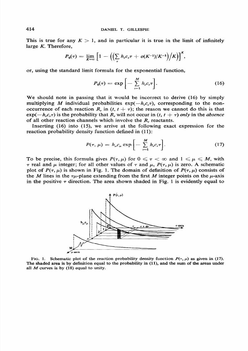
To be precise, this formula gives P(T, I*) for 0 < 7 < co and 1 < p < M, with7 real and p integer; for all other values of T and p, P(T, p) is zero. A schematicplot of P(T, p) is shown in Fig. 1. The domain of definition of P(T, CL) onsists ofthe M lines in the Tp-plane extending from the first M integer points on the p-axisin the positive T direction. The area shown shaded in Fig. 1 is evidently equal to

FIG. 1. Schematic plot of the reaction probability density function P(T, p) as given in (17).The shaded area is by definition equal to the probability in (1 ), and the sum of the areas underall it4 curves is by (18) equal to unity.




the probability in (11). We note that this probability density function is properlynormalized over its domain of definition, since

We also observe that P(T, p) depends, through the quantity in the exponential,on the reaction parameters for all reactions (not just R,) and on the currentnumbers of molecules of all reacting species not just the R, reactants).

4. THE SIMULATION ALGORITHM

The basic idea of our computational procedure is to use Monte Carlo techniquesto simulate the stochastic process described by P(,, p) in (17). Assuming that wehave access o a fast digital computer, our simulation algorithm is straightforward,and may be outlined as follows:

Step 0 (initialization). Set the time variable t = 0. Specify and store initialvalues for the N variables X, , X, ,..., X, , where Xi is the current number of mole-

cules of chemical speciesSi . Specify and store the values of the M reaction para-meters c, , c2 ..., c,,., or the M chemical reactions {R,}. Using (14), calculate andstore the M quantities h,c, , h,c, ,..., hMcM which collectively determine the reactionprobability density function P(7, CL) n (17). Finally, specify and store a seriesof “sampling times” tl < t2 < ..a, and also a “stopping time” &top .

Step 1. By employing suitable Monte Carlo techniques, generate onerandom pair (T, E.L) ccording to the joint probability density function P(T, p)in (17). Explicit methods for doing this are presented n Section 5.

Step 2. Using the numbers T and p generated in Step 1, advance t by 7,and change the {Xi) values of those species nvolved in reaction R, to reflect theoccurrence of one R, reaction. Then, recalculate the h,c, quantities for thosereactions R, whose reactant X,-values have just been changed. (For example,suppose R, is the reaction S, + S, --f 2S, . Then after replacing t by t + 7, wewould replace X, , X, and X, by X1 - 1, X, - 1 and X3 + 2, respectively; wewould then recalculate h,c, in accordance with (14) for every reaction R, in whicheither S, or S, or S, appears as a reactant.)

Step 3. If t has just been advanced through one of the sampling times ti ,

read out the current molecular population values X, , X, ,..., X, . If t > &top ,or if no more reactants remain (all h, = 0), terminate the calculation; otherwise,return to Step 1.




The computer storage spacerequired for the above procedure is evidently quiteminimal: The principle quantities which must be carried in computer memory

are the N + 2M quantities {Xi}, (c,} and {h,c,}, and it is difficult to imagine anysystem of M coupled chemical reactions involving N molecular species or whichthe required memory storage space would exceed a few hundred word locations.On the other hand, the speedof the computer is quite critical: Since each ndividualmolecular reaction is simulated in turn, the speedwith which the central arithmeticunit can execute Steps 1,2 and 3 will impose an upper limit on how many molecularreactions can be effected.This in turn limits both the number of reactant moleculesthe systemcan contain and the length of time over which the evolution of the systemcan be followed. Indeed, the maximum number of reactant molecules and the

maximum evolution time will be roughly inversely proportional to each other,and their product will be roughly proportional to the speed of the computer.Fortunately, Steps 2 and 3 are simple to execute, and, except for the few read-outsin Step 3, the computer never needs to go outside of its central memory core. Aswe shall see n the next section, the same s also true of Step 1. Therefore, in spiteof the excruciating meticulousness of our simulation procedure, modern high speedcomputers should render it practical in many nontrivial situations.

By carrying out the above procedure from time 0 to time t, we evidently obtainonly one possible realization of the stochastic process defined in (3). In order to

get a statistically complete picture of the temporal evolution of the system, wemust actually carry out several independent realizations or “runs,” each startingwith the same nitial set of molecules and proceeding to the same ime t. If we makeK runs in all, and record the quantities

Xi@, t) = the number of Si molecules found in run k at time t,(k = l,..., K) (19)

then we may assert that the average or expected number of Si molecules at time t

is [cf. (9) and (lOa)]

Xi’l’(t) N (l/K) i X,(k, t),k=l

and the root-mean-square magnitude of the f fluctuations which may reasonablybe expected to occur about this average s [cf. (9) and (lob)]

di(t) N (l/K) 2 [Xi(k, t)]” -I

(l/K) f Xi(k, t)k=l k=l

The N signs in (20) and (21) become = signs in the limit K + co. However,the fact that we obviously cannot pass to this limit of infinitely many runs is nota practical source of difficulty. On the one hand, if Ai < X “(t), then the results




&(k, t) will not vary much with k; in that case the estimate of X:“(t) would beaccurate even for K = 1. On the other hand, if d,(t) 2 X,“)(t), then a highly

accurate estimate of X/l’(t) is not really necessary; of more practical significanceand utility in this case would be the approximate range over which the numbersX,(k, t) are scattered for several runs k. In practice, somewhere between K = 3and K = 10 runs should provide a statistically adequate picture of the state ofthe chemical system at time t.

5. IMPLEMENTING THE MONTE CARLO STEP

The description of our simulation algorithm given in the preceding section iscomplete, except for the details of how to carry out Step 1. In this section we shallpresent two different procedures, which we shall call respectively the direct methodand the jirst-reaction method, for implementing this crucial “Monte Carlo step.”As we shall see,both of these methods are rigorous and exact, but if the number ofreactions M exceeds3 then the direct method should be a bit more efficient.

The term Monte Carlo is currently applied to a large and diverse collection ofcomputational procedures. A standard reference work on this many-faceted subject

is the book of Hammersley and Handscomb [9]. However, for a nonspecialist’s.introduction to the general theory and methods of generating random pointsaccording to a prescribed probability density function (which is the task beforeus here), the reader is referred to [IO, Chap. 21. Relevant portions of that referenceare summarized in our text and Appendix.

Most large digital computer facilities have available a short routine which willgenerate on call a random number (or more properly, a “pseudorandom” number)from the uniform distribution in the unit interval [ll, 121.We shall denote sucha random number by r. By definition, the probability that a generated value r will

fall inside any given subinterval of the unit interval is equal to the length of thatsubinterval, and is independent of its location:

For o<a<p<1, Prob{cu < r < j?> = /3 - CL (22)

We shall take it for granted here that we have ready access o some such “uniformrandom number generator.” Our object now is to develop methods for using theoutput values r of a uniform random number generator to generate a random pair(T, r-l>according to the probability density function P(T, p) in (17).

A. The “Direct” MethodThe first method we shall discuss is based on the fact that any two-variable

probability density function can be written as the product of two one-variable

581/22/4-2




probability density functions, a procedure known as “conditioning.” We shallcondition P(T, p) in the form

JYT, PI = PlW * P,(P I 4. (23)

Here, PI(~) do is the probability that the next reaction will occur between timest + T and t + T + dr, irrespective of which reaction it might be; and Pz(p 1 )

is the probability that the next reaction will be an R, reaction, given that the nextreaction OCCUrS at the t + 7.

By the addition theorem for probabilities, PI(~) dT is obtained by summingP(T, p) dT over all p-VdUeS; thus,

PI(T) = c” Pb, P)..L=l

Substituting this into (23) and solving for I’& 1 ) gives

pz(cL17) = P(Ts P)/$l P(T, “1.

These two equations evidently express the two one-variable density functions in(23) in terms of the given two-variable density function P(T, p). SubstitutingP(T, p) from (17) yields at once

Pi(T) = a exp(--aT) (0 < 7 < a), W)

PdP 17) = ‘%/a (CL= 1, L., Ml, (24b)

where we have for convenience abbreviated

a, = h,c, (p = 1, 2,..., M) (25)and

a E iI au = ;l h,c, . (26)

We observe in passing that, in this particular case, P,(p I T) is independent of 7.

We also note that, as we should expect, both of these one-variable density functionsare properly normalized over their respective domains of definition:

La pi(T) dT = SD a exp(--aT) dT = 1; c” P& j 7) = c” a,/a = 1.0 lL=l u=l

The idea of the “direct method” is to first generate a random value T according

to pi(T) in @la), and then generate a random integer p according to P& 1 )

in (24b). The resulting random pair (T, p) will be distributed according to P(T, P).~

5 For a formal proof and a more general discussion of this procedure, see [lo, pp. 23-351.




As we show in the Appendix (cf. (A4)), a random value T may be generatedaccording to PI(~) in (24a) by simply drawing a random number r, from the

uniform distribution in the unit interval and taking

7 = (l/a) ln(l/r,). GW

Then, as we also show in the Appendix (cf. (A7)), a random integer p may begenerated according to P,(p 1T) in (24b) by drawing another random number r2

from the uniform distribution in the unit interval and taking p to be that integerfor which

u-1

C a, -c r2a G 5 a, ;v=l v=l Wb)

i.e., the successive values a, , a2 ,... are cumulatively added (in a computer do-loop) until their sum is observed to equal or exceed r2a, whereupon p is then setequal to the index of the last a, term added.

In summary, the “direct” method for generating a random pair (7, p) accordingto P(T, CL) s to draw two random numbers r, and r2 from our uniform randomnumber generator, and then calculate T and p from (27a) and (27b), respectively.

To carry out this procedure in the most efficient manner, we should store not onlythe M quantities {a,} = {h,c,} but also their sum a. Then, in the course of updatingthe {a,,} values after each reaction, we may also update a by simply subtractingeach old a,-value and adding the corresponding new one.

Given a fast, reliable uniform random number generator, the above procedurecan be easily programmed and rapidly executed. The direct method is thereforea simple, fast, rigorous procedure for implementing Step 1 of our simulationalgorithm.

B. The “First-reaction” Method

We now present an alternate method for implementing Step 1 of our simulationalgorithm. Although this method is usually not quite as efficient as the directmethod, it is worth discussing here because of the added insight it provides intoour stochastic simulation approach.

Using the notation a, = hVcYadopted in Section 5A, it is a simple matter toshow from (13) that

P,(T) dT = exp(--a,T) * a, dT (28)

wouZd be the probability at time t for an R, reaction to occur in the time interval(t + T, t + T + dT), were it not for the fact that the number of R, reactant com-




binations might be altered between times t and t + T by the occurrence of otherreactions. This being the case, let us generate a “tentative reaction time” T, for

reaction R, according to the probability density function P, in (28), and in factdo the same or UN eactions {R”}. Thus, in accordance with (A4), we put

(v = 1, 2 ...) M), (294

where rV s a random number from the uniform distribution in the unit interval.From these A4 tentative reactions, we choose as the actual next reaction the onewhich occursjirst; i.e., we take

7 = smallest 7, for all v = 1, 2 ..., M;

p = v for which T, is smallest.V’b)

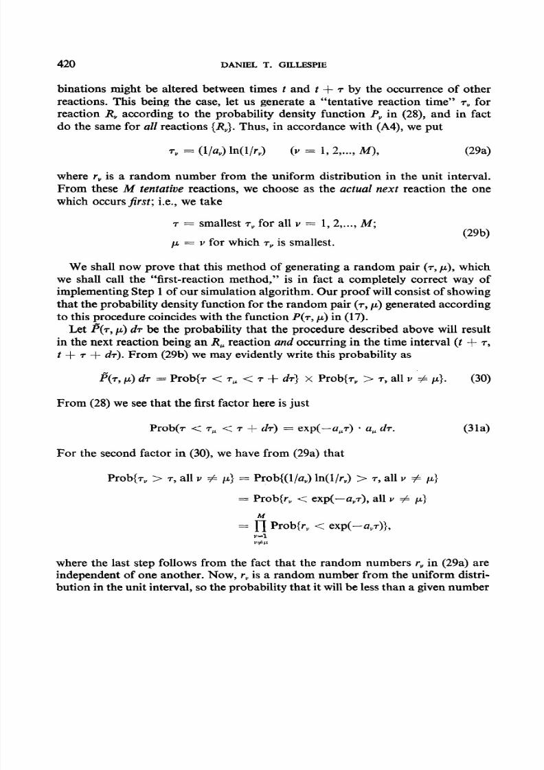
We shall now prove that this method of generating a random pair (T, ,u), whichwe shall call the “first-reaction method,” is in fact a completely correct way ofimplementing Step 1 of our simulation algorithm. Our proof will consist of showingthat the probability density function for the random pair (7, p) generated accordingto this procedure coincides with the function P(T, p) in (17).

Let P(T, tL>dr be the probability that the procedure described above will resultin the next reaction being an R, reaction and occurring in the time interval (t + T,

t + 7 + dT). From (29b) we may evidently write this probability as

&T, /a&) T = PrOb{T < 7, < 7 + dT] X Prob{T, > 7, ah v # p}. (30)

From (28) we see hat the first factor here is just

PrOb(T < r,, < 7 + dT) = eXp(-a,T) * a, dT. @la)

For the second factor in (30), we have from (29a) that

Prob{T, > T, all v # CL)= Prob{(l/a,) ln(l/r”) > 7, all v # p}

= Prob{r, < eXp(-C&T), all v # CL}

= fi Probfr, < exp(-a”T)},a-1V#U

where the last step follows from the fact that the random numbers r, in (29a) areindependent of one another. Now, rV s a random number from the uniform distri-bution in the unit interval, so the probability that it will be less han a given number



SIMULATING CXXJPLED CHEMICAL REACTIONS 421

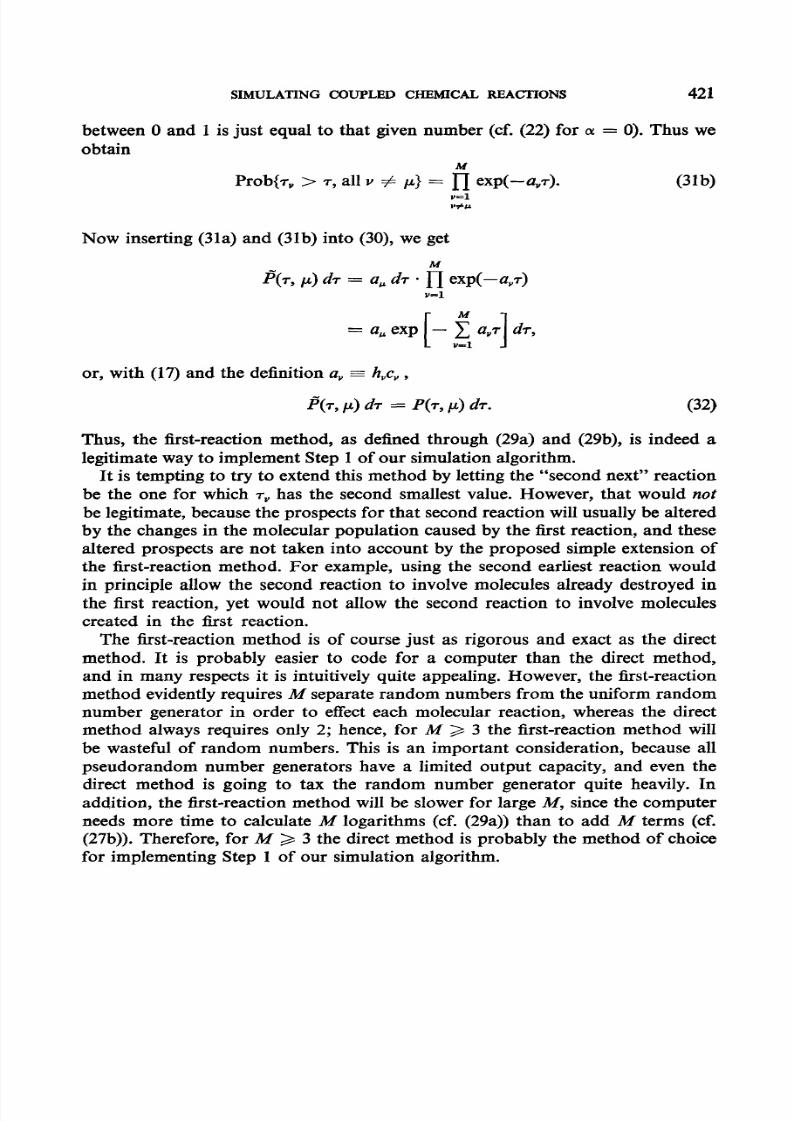
between 0 and 1 is just equal to that given number (cf. (22) for 01= 0). Thus weobtain

Prob{r” > T, all v # p} = fi exp(-aVT).v-1V#U

WV

Now inserting (31a) and (31b) into (30), we get

P(T, p) d7 = a, d7 - fi eXp(-t&T)

v=l

= a, exp

or, with (17) and the definition a, = h,c, ,

P(T, /L) dr = P(T, /L) dT. (32)

Thus, the first-reaction method, as defined through (29a) and (29b), is indeed alegitimate way to implement Step 1 of our simulation algorithm.

It is tempting to try to extend this method by letting the “second next” reaction

be the one for which 7” has the second smallest value. However, that would notbe legitimate, because he prospects for that second reaction will usually be alteredby the changes n the molecular population caused by the tist reaction, and thesealtered prospects are not taken into account by the proposed simple extension ofthe first-reaction method. For example, using the second earliest reaction wouldin principle allow the second reaction to involve molecules already destroyed inthe first reaction, yet would not allow the second reaction to involve moleculescreated in the first reaction.

The tist-reaction method is of course just as rigorous and exact as the directmethod. It is probably easier to code for a computer than the direct method,and in many respects t is intuitively quite appealing. However, the first-reactionmethod evidently requires M separate random numbers from the uniform randomnumber generator in order to effect each molecular reaction, whereas the directmethod always requires only 2; hence, for M > 3 the first-reaction method willbe wasteful of random numbers. This is an important consideration, because allpseudorandom number generators have a limited output capacity, and even thedirect method is going to tax the random number generator quite heavily. Inaddition, the first-reaction method will be slower for large M, since the computerneeds more time to calculate M logarithms (cf. (29a)) than to add M terms (cf.(27b)). Therefore, for M > 3 the direct method is probably the method of choicefor implementing Step 1 of our simulation algorithm.




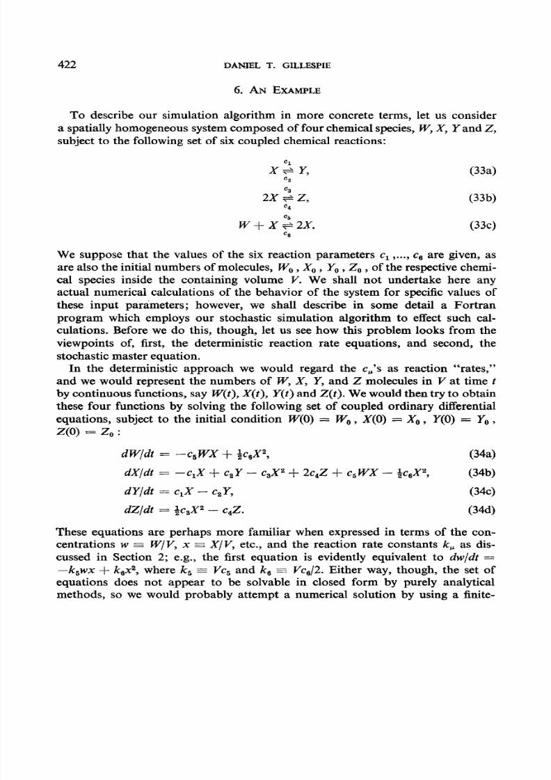
6. AN EXAMPLE

To describe our simulation algorithm in more concrete terms, let us considera spatially homogeneous system composed of four chemical species,W, X, Y and 2,subject to the following set of six coupled chemical reactions:

ClX+Y ,

52

2&z,c4

(334

(33’4

w+xzzx. % (33c)

We suppose that the values of the six reaction parameters c1 ..., c6 are given, asare also the initial numbers of molecules, W, , X0 , Y, , Z, , of the respective chemi-cal species inside the containing volume V. We shall not undertake here anyactual numerical calculations of the behavior of the system for specific values ofthese input parameters; however, we shall describe in some detail a Fortranprogram which employs our stochastic simulation algorithm to effect such cal-culations. Before we do this, though, let us see how this problem looks from the

viewpoints of, first, the deterministic reaction rate equations, and second, thestochastic master equation.

In the deterministic approach we would regard the cU’s as reaction “rates,”and we would represent the numbers of W, X, Y, and Z molecules in V at time fby continuous functions, say W(t), X(t), Y(t) and Z(t). We would then try to obtainthese four functions by solving the following set of coupled ordinary differentialequations, subject to the initial condition W(0) = W, , X(0) = X0, Y(0) = Y,, ,

Z(0) = z, :

dW/dt = -c,WX -I- &,X2, Wa)

dX/dt = -c,X + c,Y - c3X2 + 2c,Z + c5WX - &,X2, Wb)

dY/dt = c,X - c2Y, (34c)

dZ/dt = &,X2 - c,Z. (344

These equations are perhaps more familiar when expressed n terms of the con-centrations w E W/V, x = X/V, etc., and the reaction rate constants k, as dis-

cussed in Section 2; e.g., the first equation is evidently equivalent to dw/dt =

-k,wx + k,x2, where k, = Vc, and k, 3 Vc,/2. Either way, though, the set ofequations does not appear to be solvable in closed form by purely analyticalmethods, so we would probably attempt a numerical solution by using a finite-




time-step algorithm on a digital computer. However, the nonlinear character ofthe set of reactions in (33) may give rise to “multiple steady states”for certain ranges

of the input parameters [6, 7, 81; when these occur, the chemical behavior of thesystem cannot be reliably predicted within the framework of the deterministicformulation.

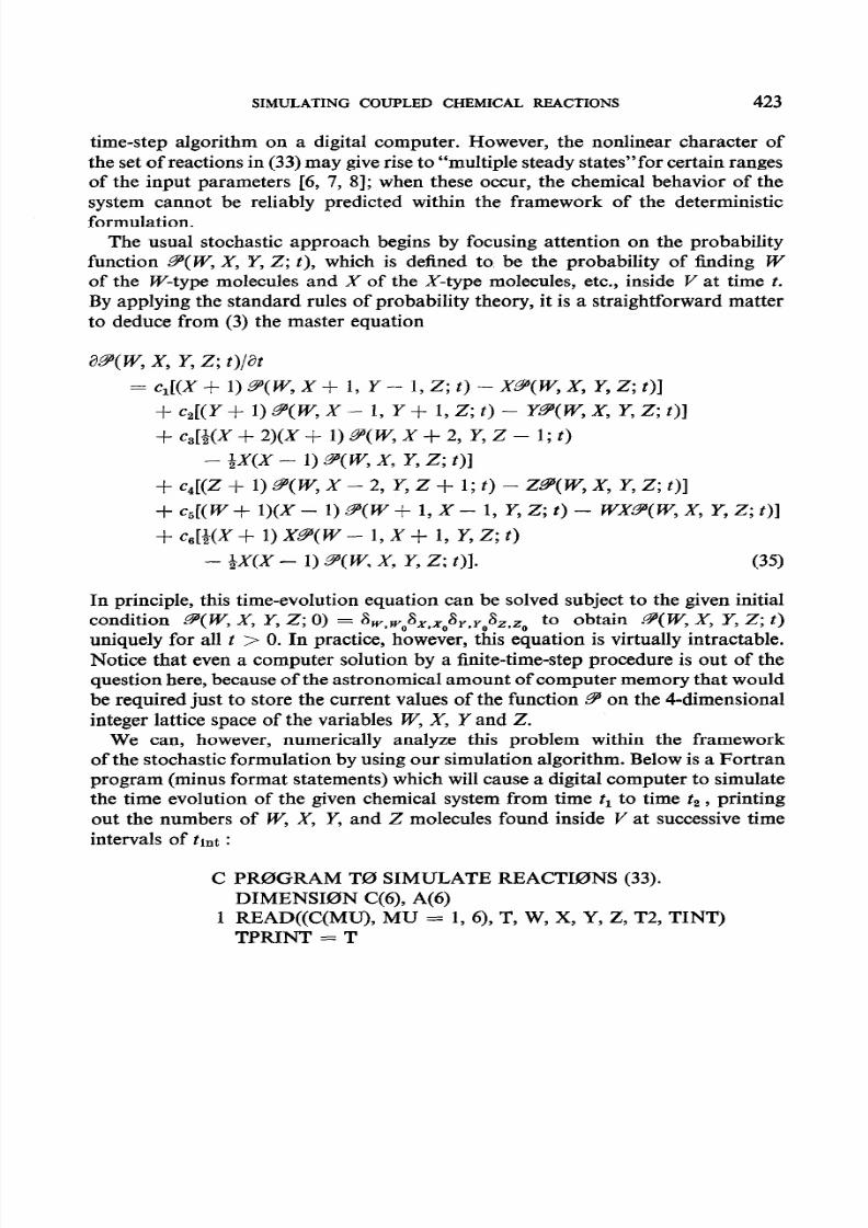
The usual stochastic approach begins by focusing attention on the probabilityfunction 9(W, X, Y, 2; t), which is defined to be the probability of tiding Wof the W-type molecules and X of the X-type molecules, etc., inside V at time t.By applying the standard rules of probability theory, it is a straightforward matterto deduce from (3) the master equation

In principle, this time-evolution equation can be solved subject to the given initialcondition sll( W, X, Y, Z; 0) = 6 6 6 6*wox,x0 Y.Y, z.z, to obtain 9( W, X, Y, Z; t)uniquely for all t > 0. In practice, however, this equation is virtually intractable.Notice that even a computer solution by a finite-time-step procedure is out of thequestion here, becauseof the astronomical amount of computer memory that wouldbe required just to store the current values of the function 9’ on the 4dimensional

integer lattice space of the variables W, X, Y and Z.We can, however, numerically analyze this problem within the framework

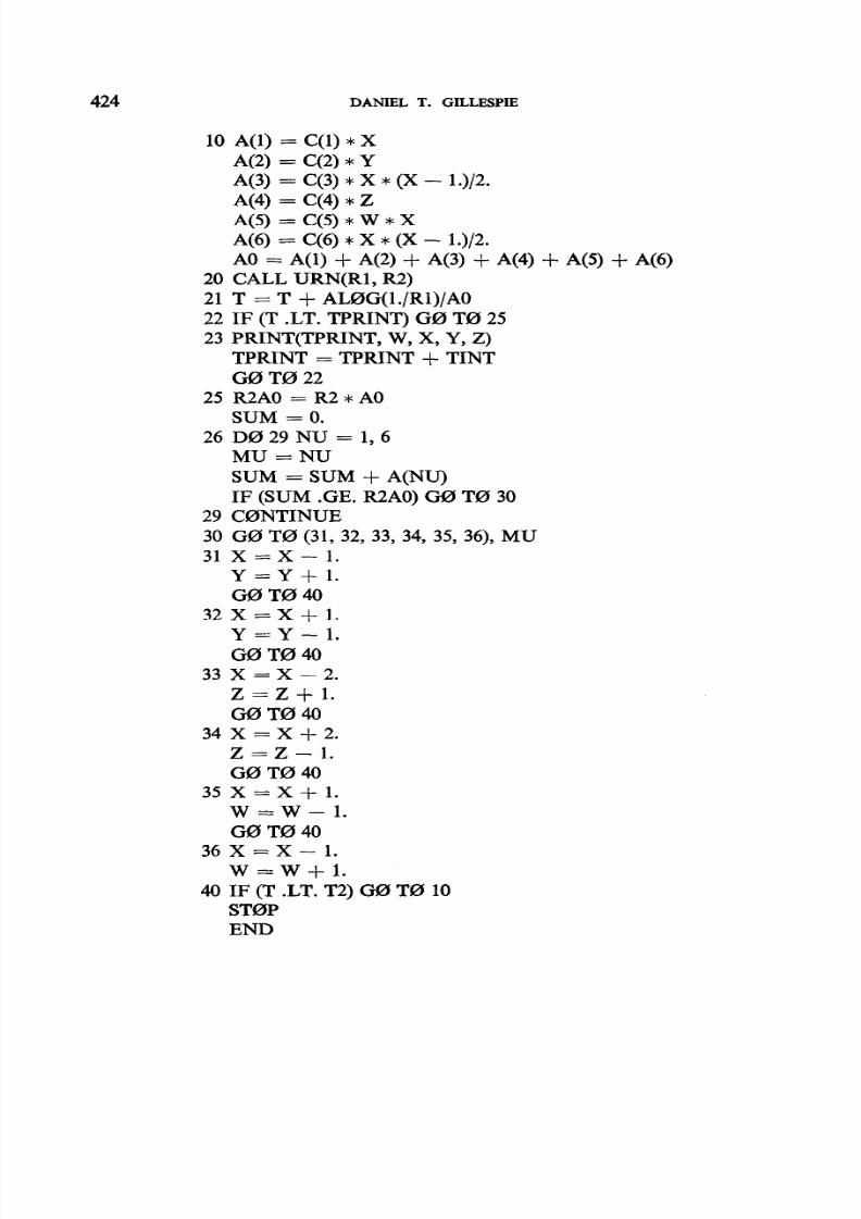
of the stochastic formulation by using our simulation algorithm. Below is a Fortranprogram (minus format statements) which will cause a digital computer to simulatethe time evolution of the given chemical system from time tl to time t2, printingout the numbers of W, X, Y, and Z molecules found inside V at successive imeintervals of tint :

C PRRIGRAM T0 SIMULATE REACTIONS (33).DIMENSI0N C(6), A(6)

1 READ((C(MU), MU = 1, 6), T, W, X, Y, Z, T2, TINT)TPRINT = T




The fact that this short, simple computer program, which requires only 27memory locations for its variables, can exactly simulate the process described

by the complicated master equation (35) illustrates a prime virtue of our simulationalgorithm. Let us now describe the workings of this program in detail.

The system’s time is denoted by the variable T, and the numbers of speciesmolecules nside Vat time Tare denoted by the respective variables W, X, Y and 2.In statement 1 the values of the externally specified parameters are read in asfollows: the six reaction parameters c, ,..., cs are read into C(l),..., C(6); the initialtime t1 is read into T; the numbers of molecules at the initial time tl are read intoW, X, Y, and Z; the stopping time tz is read into T2; and the time interval tintbetween computer printouts is read into TINT. The magnitudes of these externally

specified parameters are largely arbitrary; they will affect the total running time ofthe program, but not its memory storage requirements. Following statement 1the variable TPRINT is initialized; this variable simply keeps track of the timesat which computer printouts of the molecular population are to be made.

The main computational sequence s entered at statement 10. Here we proceedto evaluate for the current molecular population the quantities a, ,..., a, (denoted

by AU),..., A(6)) according to (25) and (14), and also the quantity Q denoted by AO)according to (26). Next, in statement 20 we call subroutine URN, which returnstwo independent random numbers Rl and R2 from the uniform distribution in the

unit interval.6 Rl and R2 correspond to the random numbers r, and r2 in the“direct method” generating formulas (27a) and (27b). In statement 21 we increasethe current value of T by the amount 7 as given in (27a); this brings the systemclock up to the occurrence time of the “next” reaction. In statement 22 we checkto see f T has ust been advanced beyond the next printout time; if it has, we printout the molecular populations at that print-out time before proceeding. (Theprogram is arranged so that the initial molecular population will always be printedout.) The determination of just which reaction R, occurs at time T is accomplishedby the seven statementsbeginning at statement 25. Here, according to the prescrip-

tion of (27b), the values a, , a2 , etc., are successively added together until theirsum is observed to equal or exceed ,a (denoted by R2AO), whereupon the reactionindex p (denoted by MU) is set equal to the index of the last a, term added. State-ment 30 then branches to the specific statements which effect the occurrence ofone R, reaction by appropriately altering the molecular population. For example,

6 See Refs. [9, 111 and (especially) [12] for ways of constructing subroutine URN for specificdigital computers. The name URN is suggested for two reasons. First, as an accronym for “UniformRandom Number Generator,” it emphasizes the sometimes unappreciated fact that “uniform-

ness” and “randomness” are not logical concomitants, and that one can also legitimately havea set of random numbers distributed according to a nonuniform or biased distribution. Second,the urn is the container traditionally used by classically refined statisticians to “hold” randomnumbers for subsequent “drawings “-precisely its function in our program.




if MU = 4 we branch to statement 34, which increases he number of X moleculesby 2 and decreaseshe number of 2 molecules by 1, in accordance with the inverse

of reaction (33b). Then, if T has not reached the stopping time T2, we return tostatement 10 to recalculate A(l),..., A(6) and A0 for the new molecular population,in preparation for the simulation of the next molecular reaction. (We have notbothered here to program around unnecessary recalculations of the A(NU)quantities; e.g., if MU = 4 on the last reaction then Y will not have been changedand A(2) need not be recalculated. For a larger system t would undoubtedly payto avoid such redundancies.) The program repeatedly cycles’from statement 10to statement 40, simulating each successivemolecular reaction in turn until Thas finally been advanced to time T2, whereupon the program terminates.

By running the program several times with the same input parameters, butdifferent initializations of subroutine URN, we may obtain means and variancesin the manner of (20) and (21). Alternatively, we may simply wish to follow thetemporal behavior of the system to see f and how a steady state is approached,and if and how transitions between multiple steady states occur. Notice that anyof the six reactions can be blocked out simply by setting its reaction parameter tozero. It is also easy to artificially hold the number of molecules of any speciesconstant; e.g., if we wished to keep the number of Y molecules constant, reflectingperhaps a very large population of Y molecules which is not appreciably affected

by the reactions, then we would simply remove the two statements ollowing state-ments 31 and 32, respectively. Clearly, a wide variety of interesting dynamicalfeatures of the set of coupled chemical reactions in (33) can be investigated withthis stochastic simulation program.

7. SUMMARY AND DISCUSSION

In this paper we have presented a relatively simple procedure for calculating the

time evolution of any spatially homogeneous chemical system in which thedynamics of the chemical reactions R, can be characterized in the manner of (3).Equation (3) is the fundamental postulate of the stochastic master equationapproach to chemical kinetics, in which the dynamics of the chemical system isregarded as a Markov process in the space of the species population numbers.In Section 2 we argued that this stochastic approach ought to be valid whenevernonreactive molecular collisions occur much more frequently than reactive

molecular collisions. We also discussed n Section 2 the relationship between thereaction parameter c, , defined in (3), and the more familiar reaction rate constant

k, , which forms the basis of the deterministic approach to chemical kinetics. Weconcluded that algebraically the relationship between c, and k, is quite simple,but conceptually c, appears to be on somewhat firmer ground than k, .




The computational procedure presented here is a systematic, computer-oriented,Monte Carlo algorithm, which directly simulates the Markov processdefined by (3).

However, the simulation algorithm is based, not on the master equation, but onthe “reaction probability density function” P(T, CL) efined in (11). Given a specifiedpopulation of molecules at time 0, the simulation algorithm is executed as follows:First, the function P(T, p) for the current molecular population is determined inaccordance with (17); second, using either of the two Monte Carlo methods (27)or (29), a pair of random numbers (7, p) is generated according to this densityfunction; and third, the time variable is advanced by T, and the molecularpopulation is adjusted to reflect the occurrence of one molecular reaction R, .By repeatedly cycling through these three steps, we may work our way from time 0

to any specified time t > 0, and thereby obtain one stochastically unbiased stateof the chemical system at time t. By examining the outcomes of several such runs,each of which starts from the same nitial state and proceeds to the same time t,

we may deduce both the mean state and time t and also the approximate magnitudeof the random jluctuations that may reasonably be expected to occur about thismean state. This computational procedure was described more concretely inSection 6, where we presented a Fortran program implementing the simulationalgorithm for a sample set of coupled chemical reactions.

Our derivation of the mathematical form of P(T, tL> from the fundamental

hypothesis (3) does not involve any additional assumptions or approximations(see Section 3). Furthermore, our methods for generating random T and p valuescommensurate with P(T, CL> re likewise completely rigorous (see Section 5 andthe Appendix). Consequently, our numerical simulation algorithm may be regardedas exact. By contrast, the commonly used numerical algorithms which solve thedeterministic reaction rate equations must be considered as approximate for tworeasons: first, the reaction rate equations themselves are approximate, relative to(3), because they ignore effects due to correlations and fluctuations; and second,virtually all numerical methods for solving sets of coupled differential equations

entail approximating infinitesimal time increments dt by finite time steps At.It turns out that, for most macroscopic chemical systems, he neglect of corre-

lations and fluctuations is a legitimate approximation [2, 31. For these cases hedeterministic and stochastic approaches are essentially equivalent, and one is freeto use whichever approach turns out to be more convenient or efficient. If ananalytical solution is required, then the deterministic approach will always be mucheasier than the stochastic approach. However, if one is forced to settle for anumerical solution, then the choice between the two approaches should be con-siderably more even. In particular, it may (or may not) turn out that our stochastic

simulation algorithm offers a convenient way around the so-called “stiffness”difficulty that occurs with the coupled differential reaction rate equations when thereaction rates range over many orders of magnitude.




For spatially homogeneous systems that are driven to conditions of chemicalinstability, correlations and fluctuations will give rise to transitions between non-

equilibrium steady states, and the usual deterministic approach is incapable ofaccurately describing the time behavior. Among the pioneering investigations intothis interesting area of chemical kinetics are the recent works of McNeil and Walls[6], Nitzan et al. [7], and Matheson et al. [8], all of whom have made use of spatiallyhomogeneous master equations to study chemical instabilities in certain simplesystems.Our stochastic simulation algorithm is directly applicable to these studies,and it should be especially useful for extending them to more complex systemsinvolving many chemical species and many highly coupled chemical reactionchannels.

The principle source of computational inaccuracy in our simulation algorithm isthe limited “randomness” of the particular unit-interval uniform random numbergenerator that is used. It is known, for example, that so-called simple multiplicativecongruential generators exhibit nonrandom pairwise correlations betweensuccessivelygeneratedvalues. Since our procedure normally usessuccessive andomnumbers in pairs to calculate the T and p values for each reaction, it would probablybe more prudent to use a “compound” multiplicative congruential generator, whichrandomly mixes two or more of the simple ones [12]. The “resolution” of thegenerator, or the number of decimal digits to which the generator can be regarded

as being effectively random, is an important consideration. For example, ann-digit generator may have trouble reliably sampling any reaction R, which hasa relative probability a,/a less han lo-“. Another important property of a uniformrandom number generator is its “period,” or how many values it will put out beforeit starts repeating itself. The period can obviously never be greater than the wordsize of the computer, but in most cases he period will be considerably less thanthis. It is not necessarily atal if the generator cycles several times during the courseof a long run, but too many cycles can obviously lead to spurious results. Thiswriter frankly regards the construction of computer codes to generate uniform

random numbers as a gray (if not black) art, which is best entrusted to expertsin the field [12]. Fortunately, the present state of this art is quite good, and willprobably improve with time.

The computer storage space equired by our simulation algorithm is quite small.This is an important consideration, since charges at most large computer facilitiesare based not only on how long a job runs but also on how much memory storageis used. However, since our algorithm simulates the occurrence of each individualmolecular reaction, it places a considerable premium on the speed of the computer.In general, the required computation time will be directly proportional to the number

of individual molecular reactions that actually take place in the system. This mustbe kept in mind when specifying the initial molecular population and the containingvolume V. Another point to bear in mind in this connection is that our algorithm,




like Nature, deals only with whole numbers of molecules; thus, for example, ifspeciesSi is to be present only in several parts per million relative to speciesS, ,

then the initial number of S, molecules should be larger than 106.It was brought to the author’s attention by one of the referees hat the simulation

algorithm presented here is similar to a computational scheme used earlier byBunker et al. [13]. In terms of present notation, Bunker et al. use the samep-selec-tion rule as n (27b), but they replace the T-selection rule in (27a) by simply T = l/u.Since l/a is precisely the mean value of the T-distribution described by PI(r)in (24a), this substitution is not unreasonable, and we may expect that in manysituations the consequent loss of fidelity will be slight enough to justify avoidingthe computational effort of generating a random number r1 and taking the

logarithm of its reciprocal; in fact, if one is interested on/y in finding the steadystates of a system, one may simply dispense with the T-selection process altogether.{Of course, the use of the mean T-step nstead of the properly randomized T-Step

will not eliminate the need to carry out several independent runs when averagesare desired.) In their paper, Bunker et al. characterize their computational pro-cedure as a “hybrid method, intermediate between differential equation solutionand Monte Carlo,” which it clearly is; however, they derive their method in aheuristic way within the context of the deterministic reaction rate formalism.By contrast, the computational procedure presented here is an “exact method,”

which has been derived in a mathematically rigorous way from very fundamentalphysical considerations. This analysis has made it quite clear that the underlyingdynamics of a chemically reacting system n thermal equilibrium is stochastic ratherthan deterministic, and consequently the stochastic approach (as exemplifiedanalytically by the spatially homogeneous master equation and numerically byour stochastic simulation algorithm) provides an intrinsically better descriptionof the system’s behavior than does the deterministic set of coupled reaction rateequations. In particular, no apologies need be made for the fluctuations that occurin a (correctly done) Monte Carlo simulation, since these fluctuations are really

present, and can in some cases give rise to macroscopically observable effects;and in those cases n which fluctuations turn out to be unimportant, that fact toowill emerge quite naturally from the calculations themselves. In a sense, then,our work here has placed the hybrid method of Bunker et al. in the context of amore rigorous framework, thus providing an a priori means of assessingts validity.Clearly, though, the procedure of Bunker et al. is intrinsically more legitimate thanany computational scheme which is based on the deterministic reaction rateequations-a point that was not obvious from their original work [13].

Finally, we make note of three possible variations or extensions of the compu-tational procedure offered here. First, we observe that the expressions for h,in (14) for the various reaction types listed in (2) follow from the definition givenin (12). However, if one has legitimate physical reasons for assuming that h, for




any reaction has a dzxerent form than required by (14), involving perhaps fractionalpowers of the numbers of reactant molecules, it is obviously a simple matter to

alter h, accordingly in our computational procedure. Indeed, it will be observedthat h, and c, are used in our simulation algorithm only in the combinationh,c, = a,, . It follows that our simulation algorithm requires onZy hat the proba-bility on the right side of (13) be expressible as a, St, where Q, can be any specified

function of the current molecular population, the physical properties of the mole-cules, and the thermal environment of the system.

Second, we note that if the temperature dependenciesof the reaction parameters(c,) are known, as for example in (6), then our simulation algorithm can be extendedto accommodate a time-varying temperature. However, any change in the

temperature must be slow enough that the entire system may always be regardedas having a single temperature, and also slow enough that the temperature changebetween successive molecular reactions be negligibly small. The temperaturechange may either be externally caused, such as the diurnal temperature changesinduced in an atmospheric chemical system; or, it may be caused by the heatabsorbed or released n the chemical reactions themselves, a phenomenon that isespecially easy to account for in our one-reaction-at-a-time approach. In eithercase, by monitoring the net heat flow into or out of the system, the system tem-perature may be constantly adjusted on the basis of an assumed system heat

capacity. The resulting temperature changes may be taken into account by peri-odically updating the reaction parameters {c,}, and the associated quantities (a,}and a, as necessary.

Finally, we describe a modification of our simulation algorithm which, althoughrather awkward, might allow one to deal in an approximate way with spatial

inhomogeneities. The basic idea is to divide the volume V into a number of sub-volumes V, (I = 1, 2,..., L) in such a way that spatial homogeneity may be assumedwithin each subvolume. Each subvolume V, would then be characterized by itsown (uniformly distributed) molecular population {XL,,>,and also a set of reaction

parameters {clsi} appropriate to the (uniform) temperature TC nside V, . Thediffusive transfer of one molecule of speciesSi from the subvolume VL to a con-tiguous subvolume V,, could be simulated by the simultaneous occurrence of thetype (2b) reaction Si -+ 0 in I/, and the type (2a) reaction * + Si in VL,

The probability coefficient a, = h,c, for this “species-i diffusive transfer reaction”might conceivably have the form




where d,,, is the center-to-center distance between subvolumes V, and V,, , All*

is the interfacing area between these two subvolumes, and Dz is an appropriately

scaled molecular diffusivity for chemical speciesSi . The transfer of thermal energybetween contiguous subvolumes might perhaps be effectedby the methods outlinedin the preceding paragraph. The dynamics of the system as a whole would begoverned by a suitably generalized form of the reaction probability density function.One likely candidate for this would be the function defined by

P(T, p, I) d7 = probability at time t that the next reaction in V willoccur in the time interval (t + T, t + 7 + d7), and (37)will be an R, reaction inside the subvolume V, .

The simulation would then proceed by applying our Monte Carlo methods togenerate random triplets (T, p, r) according to this three-variable probability densityfunction. For extensive, complicated systems this approach would probably beimpractical because of the large number of subvolumes required and the resultingplethora of reaction channels, particularly those channels controlling diffusivetransfers between contiguous subvolumes. However, this approach might be quitefeasible for a system confined to a tubular volume in which the gradients are smalland entirely along the tube axis; in that caseeach subvolume would have only twoneighbors. For the present, though, attempts to extend our simulation algorithmto spatially inhomogeneous systems seem rather premature, and probably shouldawait a more precise determination of the domain of feasibility of the algorithmfor spatially homogeneous systems.

APPENDIX: THE INVERSION GENERATING METHOD

Equations (27a), (27b), and (29a) are applications of a general Monte Carlo

technique called the “inversion method,” whereby one uses random numbersfrom the uniform distribution in the unit interval (see (22)) to construct randomnumbers distributed according to any prescribed probability density function.In this Appendix we review this well-known generating technique for both con-tinuous-single-variable and discrete-single-variable probability density functions.The application of the inversion method to multivariable probability densityfunctions is discussed n [lo, Chap. 21.

Suppose we wish to generate a random real number x according to the proba-bility density function P(x). By definition, P(Y) dx’ is to be the probability that x

will lie between x’ and x’ + dx’. Consider the function

F(x) z /* P(x’) dx’.-m

641)




Evidently, I;(x,,) is the probability that x will be less than x,, . The function F(x)defined by (Al) is called the probability distribution function, and is to be clearly

distinguished from the probability density function P(x). Notice that

F(-co) = 0 and F(+oo) = 1; WI

the second equality is the “normalization condition,” which expresses he factthat every random x has got to be someplace.Notice also that, since P(x) is every-where nonnegative, then (Al) implies that F(x) rises from 0 at x = -cc to 1 atx = + co in a nondecreasing way.

The inversion method for generating a random value x according to a given

density function P(x) is simply to draw a random number r from the uniformdistribution in the unit interval, and take for x that value which satisfiesF(x) = r;

in other words, take

x = F-l(r), (A3)

where F-l is the inverse of the distribution function corresponding to the givendensity function P. (Note that the range and monotonicity of F(x) insure theexistence of F-l(r) in 0 < r < 1.)

To prove that this procedure is correct, let us calculate the probability that the

x-value so generated will lie between x’ and x’ + dx’. By construction, thisprobability is the same as the probability that r will lie between F(x’) andF(x’ + dx’). Since r is a random number from the uniform distribution in the unitinterval, then by (22) this probability is just

F(x’ + dx’) - F(x’) = F’(x’) dx’ = P(x’) dx’,

where the second equality follows from (Al). We conclude, then, that the proba-bility density function for the random number x generated according to (A3) isindeed P(x).

For example, suppose we wish to generate a random number x according to theprobability density function

P(x) = A exp(--dx), for 0 < x < cc,

= 0, otherwise,(AW

where A is a positive constant. Using (Al), we easily calculate the correspondingprobability distribution function to be F(x) = 1 - exp(--dx). Then putting

F(x) = r and inverting (and for simplicity replacing the random variable 1 - rby the statistically equivalent random variable r), we obtain

x = (l/A) ln(l/r) (A4b)




as the rule for generating a random number x according to the probability densityfunction P(X) in (A4a). This is the formula used n (27a) and (29a).

In the discrete case, he problem is to generate a random integer i according tothe probability density function P(i), where P(i’) is now the probability that i

will equd i’. The corresponding distribution function F(i) is defined by

F(i) = i P(i’),(‘=-UI

(A%

and F(i,) is evidently the probability that i will be less than or equal to i,, .

The inversion method for generating i according to P(i) is to draw a random

number r from the uniform distribution in the unit interval and take for i that valuewhich satisfies

F(i - 1) -=c < F(i). 646)

To prove that this procedure is correct, let us calculate the probability that theresulting integer i will equal i’. This probability is just the probability that r willlie betweenF(i’ - 1) and F(C), and by (22) this probability is

F(i’) - F(i’ - 1) = i P(Y) - ‘< P(Y) = P(i’).i’=--m i”---m

This proves that P(i) is indeed the probability density function for the randomnumber i generated according to the rule (A6).

For example, suppose we wish to generate a random integer i according to thedensity function

P(i) = aJ5 a, ,j=l

for i = 1, 2 ..., M,

= 0, otherwise,

where the ai’s are nonnegative numbers. Then applying (A6) we see hat we mustchoose i to be that integer for which

i-l

izl W'> < r G jl W>

WV

This is the generating formula used in (27b).

SSdd4-3




1. D. A. MCQUARRIE, J. Appl. Probability 4 (1967), 413.2. I. QPPENHEIM, K. E. SHULnR, AND G. H. WEISS, J. Chem. Phys. 50 (1969), 460.

3. T. G. KURTZ, J. Chem. PhyJ. 57 (1972), 2976.

4. R. D. PRESENT, “Kinetic Theory of Gases,” Chap. 8, McGraw-Hill, New York, 1958.

5. J. H. Gmas AND P. D. FLEMING, J. Statist. Phys. 12 (1975),375.6. K. J. McNE~ AND D. F. WALLS, J. Statist. Phys. 10 (1974), 439.

7. A. NITZAN, P. ORTOLEVA, J. DEUTCH, AND J. Ross, J. Chem. Phys. 61(1974), 1056.

8. I. MATH~~N, D. F. WALLS, AND C. W. GARIXNER, J. Statist. Phys. 12 (1975), 21.

9. J. M. HAMME~~LEY AND D. C. HANDSCOMB, “Monte Carlo Methods,” Me&men, London,

1964.

10. D. T. GILLESPIE, NWC TP 5714 “The Monte Carlo Method of Evaluating Integrals,” Naval

Weapons Center, China Lake, Calif., 1975. (Available through the National Technical In-

formation Service, Sprin+$ield, Va. 22161.)

11. R. P. CHAMaERS, IEEE Spectrum 4 (1967), 48.12. G. MAR~AGLIA AND T. A. BRAY, Comm. ACM 11(1968),757.

13. D. L. BUNKER, B. GARRETT, T. KLEINDIENST, AND G. S. LONG III, Combust. FZame23 (1974),

373.

gillespie general method

Documents