gerald l. wallace jr., bs, mba - era home
TRANSCRIPT

This thesis has been submitted in fulfilment of the requirements for a postgraduate degree
(e.g. PhD, MPhil, DClinPsychol) at the University of Edinburgh. Please note the following
terms and conditions of use:
• This work is protected by copyright and other intellectual property rights, which are
retained by the thesis author, unless otherwise stated.
• A copy can be downloaded for personal non-commercial research or study, without
prior permission or charge.
• This thesis cannot be reproduced or quoted extensively from without first obtaining
permission in writing from the author.
• The content must not be changed in any way or sold commercially in any format or
medium without the formal permission of the author.
• When referring to this work, full bibliographic details including the author, title,
awarding institution and date of the thesis must be given.

Decisions of Capital Structure in the
Presence of Agency and Collusive
Monopsony
A Study of the U.S. Acute Care Hospital Market
Gerald L. Wallace Jr., BS, MBA
University of Edinburgh College of Humanities and Social Science
The Business School
A thesis submitted for examination for the degree of Doctorate of Philosophy (PhD)
The University of Edinburgh
August 2011
Post Viva Corrections
April 30th 2012

2
Declaration of Gerald L. Wallace, Jr.
Upon submission of this thesis for a degree of Ph.D. in Finance to
The University of Edinburgh College of Humanities and Social Sciences
I, Gerald Leon Wallace, Jr., declare that the thesis composed in effort
of this degree is my own work and has been composed myself. Any and all
work associated with construction of the thesis was provided by me with the
exception of those efforts outlined in the acknowledgements.
The work submitted in this thesis has not been submitted for any other
degree or professional qualification.
Gerald Leon Wallace, Jr.
Candidate for PhD Finance
3
Abstract
The United States acute care hospital (ACH) market provides a unique
environment in which to examine questions about market structure and performance.
The ACHs operate in a mature market of health services that is highly regulated and
has one dominant primary consumer of services. The uncharacteristic industry
structure offers the opportunity to analyze pervasive agency relationships and capital
structure issues in a new setting. In addition, the policies of the U.S. Government have
created an environment in which tacit collusion is likely to flourish, which leads to
market buyer power (monopsony, or buyers acting as one monopoly buyer). A key
question is the extent to which monopsony and agency affect capital structure
decisions. Agency is defined by Ross (1973, p.134) as a relationship formed between
a principle and their agents, “when one, designated as the agent, acts for, on behalf of,
or as representative for the other, designated the principal, in a particular domain of
decision problems.” This thesis extends the agency framework provided by Jensen
and Meckling (1976), along with the econometric understanding of monopsony in
healthcare via tacit collusion, as suggested by Pauly (1998) and Sevilla (2005), and
the research constraints of monopsony under an all-or-nothing contract, as outlined by
Taylor (2003).
Using data on ACHs from the period of 1995 to 2007 for approximately 5,000
ACHs, which was derived from the Medicare Cost Report and medical payments for a
sub-population of 1,500, this research examines the determinants of capital structure
in a distorted market. Building upon this initial analysis, the research seeks to
examine the effects of market distortions upon free cash flow, and ultimately, capital
structure. Two theories of distortion are presented that would affect free cash flow:
The first is that of the agency cost of free cash flow and signaling, and the second is a
theory of monopsony via tacit collusion between buyers.
A model of the agency relationship between ACHs and the U.S. Government
is proposed, promoting agency cost (signaling and the agency cost of free cash flows)
as a causal relation with free cash flows and capital structure (Jensen & Meckling
1976; Jensen 1986). Empirical models of agency are constructed, examining the
dependence on government business and the relation to the leverage (signaling) and
free cash flows (agency cost of free cash flows) for ACHs. In addition, a

4
complementary theory of capital structure determinant via market power
(monopsony) is formulated, suggesting that monopsony conditions within the ACH
market affect free cash flows and capital structure. The analysis provides a framework
for understanding the environments in which ACHs operate and the strength of
bargaining within the market. The research concludes with a review of the
determinants of capital structure in light of the inefficiencies and distortions of the
industry and the relationships observed.

5
Dedication
I dedicate this thesis to my late father, Dr. Gerald L. Wallace, Sr., who
provided me with such love and inspiration as a child. I truly appreciate him, and will
love and miss him always.

6
Acknowledgements
This thesis has been a long road to enlightenment, with many hours of reading,
contemplation, and writing. I have been tormented by problems and ideas,
emboldened by solutions, and educated by the process. I truly am thankful for the
opportunity to submit this thesis. It has taken many long hours interfacing with many
different people to make this research a success. I would like to thank some of those
people that helped and supported me in this process.
My first thanks are to God and his son Jesus Christ, for giving me the
capability to achieve great things. My thanks go to my lovely wife, Melissa; without
her support, this research would not have been possible. She has tolerated me
uprooting my family and moving them to Scotland for a number of years, my long
hours when I was sequestered in my office, and a general lack of intelligence on my
part at all times. I would like to thank my children for giving me solace from my
work when things became difficult, and for their undying love for their father. It is
for our children that we conquer all mountains.
I want to acknowledge my mother and father for instilling an unquenchable
thirst for knowledge and the drive and determination to see this educational journey to
its end.
The research would not be possible were it not for the direction and input of
Dr. Peter Moles, without whom this Ph.D. would not have come to fruition. His
direction, tutelage, and comments greatly have improved the quality of this work. My
thanks for his patience and for the long hours of dialogue over endless subject matters
related to this research. I am indebted to him for helping me achieve greater
enlightenment in the process of creating this thesis. In addition, I would like to thank
Jonathan Crook for his invaluable advice on my research questions, and for solutions
to some of my most challenging quandaries. I owe many thanks to John Banasik for
his clarity and willingness to support me on all matters of statistics, not to mention his
witty banter.
This research would not have been possible without the support and
cooperation of those at The SSI Group, Inc. Debbie Short was masterful in
understanding the layout and concept of the research, and she was helpful in orienting
the claims data that made the research possible. Kimberly Scaturro was extremely
helpful to me in helping me manipulate and orient the claims data within the SQL
database. The intricate combination of both public and private data within the SQL
database made this research possible, and it could not have been accomplished
without these two ladies. I am grateful eternally for their support and patience in this
process. In addition, I would like to thank Lamar Windham, who provided the
technical support needed to make the long distance computing possible. There were
long nights and endless days of computing with emails and calls at all hours of the
day and night, and he answered them all.
Many thanks to the team at Springhill Medical Center who helped me to
understand and refine my methodology of coding the health procedures, ICD9, and
for helping me in choosing procedures to use in the research. This includes Melanie
Sigler and Sharon Barnicle. Thanks to the technical support team of Troy Hopkins
and Steve Drake.
Thanks to Celia Wallace, Dr. Ken Ellingwood, Dr Semoon Chang, Melissa
Wallace and others for providing feedback on the thesis

7
Table of Contents
Abbreviations ..................................................................................................... 10
Tables &Figures ..................................................................................................... 11
1. Introduction ................................................................................................... 19
1.1 Research in Literature ............................................................................ 20
1.2 Advantages of The Research ................................................................. 22
1.3 Description of The Data ......................................................................... 23
1.4 Agency Theory....................................................................................... 24
1.5 Testing for Agency Cost ........................................................................ 26
1.6 Collusive Monopsony ............................................................................ 27
1.7 Testing for Collusive Monopsony ......................................................... 28
1.8 Research Findings .................................................................................. 29
1.9 Contributions.......................................................................................... 30
1.10 Thesis Structure ..................................................................................... 32
2. History and Structure of the Acute Care Hospital Market ............................ 34
2.1 History.................................................................................................... 34
2.2 Current Political Climate ....................................................................... 41
2.3 Mechanics of Healthcare: Financing and Delivery ................................ 44
2.4 U.S. Healthcare Regulation a Functional Discussion ............................ 50
2.5 Acute Care Hospitals an Environment for Analysis .............................. 53
2.6 Conclusion ............................................................................................. 55
3. Liquidity and Capital Structure Trends ......................................................... 57
3.1 Introduction ............................................................................................ 57
3.2 Background (History and Literature) ..................................................... 58
3.3 Data ........................................................................................................ 60
3.4 Methodology .......................................................................................... 67

8
3.4.1 Introduction ............................................................................................ 67
3.4.2 Ratios to Be Used in the Analysis.......................................................... 69
3.5 Results .................................................................................................... 72
3.6 Conclusion ............................................................................................. 88
4. Agency .......................................................................................................... 92
4.1 Introduction ............................................................................................ 92
4.2 Agency Theory..................................................................................... 105
4.3 Data ...................................................................................................... 120
4.4 Models................................................................................................. 134
4.5 Results .................................................................................................. 140
4.7 Conclusions .......................................................................................... 149
5. Monopsony in Healthcare and Literature .................................................... 156
5.1 Introduction .......................................................................................... 156
5.1.1 Theory of Monopsony.......................................................................... 157
5.2 Monopsony in Literature...................................................................... 168
5.3 Conclusion ........................................................................................... 184
6. Empirical Evidence of Collusive Monopsony ............................................ 186
6.1 Introduction .......................................................................................... 186
6.2 Data ..................................................................................................... 188
6.3 Data Organization, Behavior, and Sample Creation ............................ 191
6.4 Methodology ........................................................................................ 199
6.5 Results .................................................................................................. 217
6.6 Conclusion ........................................................................................... 239
6.7 Contributions to Knowledge ................................................................ 242
7. Thesis Summary and Conclusion ................................................................ 243
7.1 Agency Costs ....................................................................................... 243
7.2 Collusive Monopsony ................................................................................ 244

9
7.3 Implications.......................................................................................... 246
7.4 Contributions of the Research .................................................................... 252
7.5 Limitations of the Research ....................................................................... 254
7.6 Recommendations for Further Research .................................................... 256
Appendix .............................................................................................................. 280
3.5.1 Profitability Ratios ............................................................................... 280
Chapter 3 Variable Nomenclature and Definitions .......................................... 330
Chapter 4 Variable Nomenclature and Definitions .......................................... 331
Chapter 4 .............................................................................................................. 332
Chapter 6 Geometric Length of Stay ................................................................... 340
Chapter 6 Procedures ........................................................................................... 341
(exploratory, outliers, and data adjustments) ....................................................... 341
Chapter 6 Appendix (Panel Data Regression Models)...................................... 372

10
Abbreviations
ACH- Acute Care Hospital
MCR- Medicare Cost Report
CMS- Centers for Medicare and Medicaid Services
DOJ- U.S. Department of Justice
FCF- Free Cash Flows
KPF- Kaiser Permanente Foundation
HMO- Health Maintenance Organization
GDP- Gross Domestic Product
HHI- Herfindahl Hirschman Index
NISP- Net Income from Service to Patients
LI- Lerner’s Index
PPO- Preferred Provider Organization
PSRO- Professional Standards Review Organization
MCO- Managed Care Organization
DRG- Diagnosis Related Grouper
HCRIS- Healthcare Provider Cost Reporting Information System
CPI- Consumer Price Index
PCP- Primary Care Physician
NEIO- New Empirical Industrial Organization
NPV- Net Present Value
AHA- American Hospital Association
AMA- American Medical Association
CCMC- Committee on the Cost of Medical Care
GHA- Group Health Association
AMA- American Medical Association
CHIP- Children’s Healthcare Insurance Program
HIPPA- Health Insurance Portability & Accountability Act
PPS- Prospective Payment System
MS SQL- Microsoft SQL Database
GAAP- General Acceptable Accounting Principles
ROA- Return on Assets
ROE- Return on Equity
AR- Accounts Receivable
DSO- Days Sales Outstanding
DCOH- Days Cash on Hand
FATR- Fixed Asset Turnover
JACHO- Joint Commission on Accreditation of Hospitals
ANOVA- Analysis of Variance
FA- Fixed Assets
OCF- Operation Cash Flows
CAPEX- Capital Expenditures
GMLOS- Geometric Length of Stay
LnTA- Natural Log of Total Assets
GMM- Generalized Method of Moments
SMSA- Standard Metropolitan Statistical Area
RBRVS- Resource Based Relative Value Scale
PCP- Primary Care Physicians
MSA- Metropolitan Statistical Area
ATC- Average Total Cost
AVC- Average Variable Cost
AC- Average Cost
11
Tables &Figures
Figure 3.1: Histogram N Cases by Fiscal Year..................................................... 62
Figure 3.2: Population Outline by Hospital Size. .................................................. 63
Table 1: ACH Category by Bed Size: .................................................................... 63
Integer values represent the number of beds in each ACH. The number of beds
was identified with the variable “num_beds” from the MCR................................ 63
Table 3.2: Sample Descriptive for Each Ratio, Pre- and Post-Removal of Outliers.
................................................................................................................................ 68
Table 3.3: The Seven Basic Financial Factors and Recommended Ratios, by Chen
and Shimerda (1981), along with description and equation for each. ................... 69
Table 3.4: Ratios Used to Determine Hospital Failure by Previous Researchers,
divided by authors’ ratio preference: ..................................................................... 71
Table 3.5: Ratios for This Research with Description and Equations. .................. 72
Figure 3.4: Mean Profitability Ratios by Fiscal Year Reported: ........................... 76
Table 3.5: Mean Ratios by Fiscal Year Reported. ................................................ 77
Table 3.6: ACH Financial Ratios by ACH Size Category: .................................... 78
Figure 3.5: Mean Profitability Ratios by Size Return on Equity and Return on
Assets: .................................................................................................................... 79
Figure 3.6: Leverage Ratios by Fiscal Year Reported : ......................................... 80
Figure 3.7: Leverage Ratios by ACH Size Category: ............................................ 81
Figure 3.8: Mean DSO and Cash Ratio by Fiscal Year Reported: ........................ 82
Figure 3.9: DSO and DCOH by Fiscal Year Reported: ......................................... 83
Figure 3.10: The DSO and DCOH by Fiscal Year Reported:................................ 84
Figure 3.11: Liquidity Ratios by Fiscal Year Reported: ........................................ 85
Figure 3.12: Liquidity Ratios by ACH Size........................................................... 86
Figure 3.13: Fixed Asset Turnover Ratio by Fiscal Year Reported: ..................... 87
Figure 3.14: Fixed Asset Turnover by ACH Size Category.: ............................... 88
Figure 3.15: Mean DCOH, DSO, and Cash Ratio by Fiscal Year Reported: ........ 89
Figure 4.1: Signaling Variables: .......................................................................... 123
Table 4.1: Correlation Matrix for Variables in Signaling Regression: ................ 124
Table 4.2: Statistical Descriptives of Signalling Variables: ................................ 124
Table 4.4: Correlation Matrix for Agency Cost FCF Variables in Regression: . 130

12
Table 4.5 Statistical Descriptives of Agency Cost of Free Cash Flow Variables:
.............................................................................................................................. 130
Table 4.3: Signaling Models: ............................................................................... 141
Table 4.4: Agency Cost of FCF Models: ............................................................. 144
Figure 5.1: Monopsony Welfare Loss: ................................................................ 158
Figure 5.2: All-or-Nothing Monopsony Model: .................................................. 160
Table 6.1: Monopsony Study Clinical Procedures (DRG = Diagnosis Related
Grouper) (ICD9= International Classification of Deseases):............................... 192
Figure 6.2: Procedure Name and Definition: ....................................................... 195
Figure 6.4: Case Count by Year and Payer: ........................................................ 196
Figure 6.5: Mean Reimbursement by Year and Payer ......................................... 197
Figure 6.6: Procedure Name, Descriptives, and Outliers: ................................... 198
Table 6.2: Summary Statistics for all variables included in the Lerner’s Index
Regressions: ......................................................................................................... 206
Table 6.3: Correlation Matrix for Lerner’s Index Variables: .............................. 206
Table 6.4: Summary Statistics for all variables included in the Herfindahl-
Hirschman Index: ................................................................................................. 214
Figure 6.13: Lerner’s Index Descriptives by Fiscal Year: ................................... 218
Figure 6.14: Lerner’s Index Random Effects: ..................................................... 219
Figure 6.15: Histogram HHI (2000-2007): .......................................................... 222
Figure 6.16: Box Plot of Payor Count (2000-2007): ........................................... 223
Figure 6.17: Payer Count Histogram (2000-2007): ............................................. 224
Figure 6.20: Scatter Plots Payor_Count by Hospital Size by Number of Beds
(ABOVE): ............................................................................................................ 225
Figure 6.21: Scatter Plot of Concentration (HHI) vs. Hospital Size (number of
beds): .................................................................................................................... 226
Figure 6.22: Mean Payer Count by Year (1995-2007) ........................................ 227
Table 6.6: HHI Maximum Competitiveness Values as Determined by Payor Count
.............................................................................................................................. 227
Table 6.7: Efficient (minimum) HHI Possible to Actual Mean HHI by Fiscal Year
Reported: .............................................................................................................. 229
Figure 6.23: Comparison of Actual HHI vs. Theoretical Competitive HHI: ....... 230
Chapter 3 Definitions, Ratios and Equations ....................................................... 280
13
Figure 3.1A: Histogram ROE no limitations ....................................................... 281
Figure 3.2A: ROE box plot, no limitation ........................................................... 281
Figure 3.3A: Histogram ROE w/limitation (-0.26, 0.42) ..................................... 282
Figure 3.4A: Boxplot ROE w/limitation (-0.26, 0.42) ......................................... 282
Table 3.2A: Desciptive statistics for Return on Equity by year w/limitation (-0.26,
0.42) ..................................................................................................................... 283
Table 3.3A: Descriptives of Return on Equity by Hospital Size w/limitation (-
0.26, 0.42) ............................................................................................................ 283
Figure 3.5A: Histogram RoA (N) with no limiters .............................................. 284
Table 3.4A: Desciptive Statistics Return on Assets (RoA -X, denotes removal of
outliers) ................................................................................................................ 285
Figure 3.6A: Histogram RoA (n) with limitation @ (-0.15, 0.22) ....................... 285
Figure 3.7A: Box plot RoA (n) with limitation @ (-0.15,0.22) ........................... 286
Table 3.5A: Descriptive statistics for Return on Assets by year limited @ (-0.15,
0.22). .................................................................................................................... 286
Table 3.6A: Descipritives for Return on Assets by hospital size limit @ (-0.15,
0.22). .................................................................................................................... 287
Figure 3.8A: Histogram Net Margin with no limitation ...................................... 288
Figure 3.9A: Box plot Net Margin with no limitation ........................................ 288
Table 3.7A: Descriptive statistics for Net Margin ( Net Margin -X, denotes
removal of outliers). ............................................................................................. 289
Figure 3.10A: Histogram Net Margin w/limits (-0.80, 0.118) ............................. 289
Figure 3.11A: Box plot Net Margin w/limits (-0.80, 0.118) ................................ 290
Table 3.8A: Descriptives for Net Margin by fiscal year w/limits (-0.80, 0.118). 290
Table 3.9A: Descriptives for Net Margin by hospital size w/limits (-0.80, 0.118).
.............................................................................................................................. 291
Figure 3.12A: Histogram Operating Margin (N) with no limitation ................... 291
Figure 3.13A: Box Plot Operating Margin (N) with no limitation ...................... 292
Table 3.10A: Descriptives for Operating Margin ( Oper Margin-X, denotes
removal of outliers). ............................................................................................. 292
Figure3.14A: Histogram Operating Margin w/limitation (-0.26, 0.23) ............... 293
Figure 3.15A: Box plot Operating Margin w/limitation (-0.26, 0.23) ................. 293
14
Table 3.11A: Descriptive statistics for Operating Margin by fiscal year
w/limitation (-0.26, 0.23). .................................................................................... 294
Table 3.12A: Descriptives for Operating Margin by hospital size. ..................... 294
Figure 3.16A: Histogram Debt Ratio with no limitations.................................... 295
Figure 3.17A: Box plot Debt Ratio with no limitations ....................................... 296
Figure 3.18A: Histogram Debt Ratio w/limits (-0.39, 1.34) ............................... 296
Table 3.13A: Descriptive statistics for Debt Ratio (Debt Ratio-X, denotes removal
of outliers). ........................................................................................................... 297
Figure 3.19A: Box plot Debt Ratio w/limits (-0.39, 1.34) ................................... 297
Table 3.14A: Descriptive statistics for Debt Ratio by fiscal year w/limits (-0.39,
1.34). .................................................................................................................... 298
Table 3.15A: Descriptives for Debt Ratio by hospital size w/limits (-0.39, 1.34).
.............................................................................................................................. 298
Figure 3.20: Histogram Debt to Equity with no limitations ................................ 299
Figure 3.21A: Box plot Debt to Equity with no limitations ................................ 300
Figure 3.22A: Histogram Debt to Equity w/limits (-1.5,3.2)............................... 300
Table 3.16A: Descriptives for Debt/Equity Ratio (Debt/Equity-X, denotes removal
of outliers). ........................................................................................................... 301
Figure 3.23A: Box plot Debt to Equity w/limits (-1.5, 3.2)................................. 301
Figure 3.24A: Mean Debt to Equity by Fiscal Year Reported w/limits (-1.5, 3.2)
.............................................................................................................................. 301
Table 3.17A: Descriptives for Debt to Equity Ratio by fiscal year w/limits (-
1.5.3.2). ................................................................................................................ 302
Table 3.18A: Descriptives for Debt to Equity Ratio by hospital size w/limits (-
1.5.3.2). ................................................................................................................ 303
Figure 3.25A: Histogram Days Cash on Hand with no limitation ....................... 303
Figure 3.26A: Box plot Days Cash on Hand with no limitation .......................... 304
Figure 3.27A: Histogram Days Cash on Hand w/limitation (-160,275) .............. 304
Table 3.19A: Descriptives for Days Cash on Hand (DCOH -X, denotes removal of
outliers). ............................................................................................................... 305
Figure 3.28A: Box plot Days Cash on Hand w/limitation (-160,275) ................. 305
Table 3.20A: Descriptives for Days Cash on Hand by fiscal year w/limitation (-
160, 275) .............................................................................................................. 306
15
Table 3.21A: Descriptives for Days Cash on Hand by hospital size w/limitation (-
160, 275). ............................................................................................................. 306
Figure 3.29A: Histogram Cash Ratio with no limitation ..................................... 307
Figure 3.30A: Box plot Cash Ratio with no limitation ....................................... 308
Table 3.23A: Descriptives of the Cash Ratio (Cash Ratio-X, denotes removal of
outliers). ............................................................................................................... 308
Figure 3.31A: Histogram Cash Ratio w/limitation (-2.1, 7.1) ............................. 309
Figure 3.32A: Box plot Cash Ratio w/limits (-2.1, 7.1) ...................................... 310
Table 3.24A: Descriptives for the Cash Ratio by fiscal year w/limitation (-2.1, 7.1)
.............................................................................................................................. 311
Table 3.25A: Descriptives for the Cash Ratio by hospital size w/limits (-2.1, 7.1).
.............................................................................................................................. 311
Figure 3.33A: Histogram Current Ratio with no limitations ............................... 312
Figure 3.34A: Box plot Current Ratio with no limitations .................................. 312
Table 3.26A: Descriptives for the Current Ratio (Current Ratio-X, denotes
removal of outliers). ............................................................................................. 313
Figure 3.35A: Histogram Current Ratio with Limitation (-1.4, 5.8) ................... 314
Figure 0.1.36A: Box plot of Current Ratio w/limitations (-1.4, 5.8) ................... 314
Table 3.27A: Descriptives for the Current Ratio by fiscal year w/limitations (-1.4,
5.8). ...................................................................................................................... 315
Table 3.28A: Descriptives for the Current Ratio by hospital bed size w/limits (-
1.4, 5.8) ................................................................................................................ 315
Figure 3.37A: Histogram Quick Ratio w/no limitations ...................................... 316
Figure 3.38A: Box plot Quick Ratio w/no limitations ......................................... 317
Table 3.29A: Descriptives for the Quick Ratio (Quick Ratio-X, denotes removal
of outliers). ........................................................................................................... 317
Figure 3.39A: Histogram Quick Ratio w/limitations (-1.3, 5.4) .......................... 318
Figure3.40A: Box plot Quick Ratio w/limits (-1.3, 5.4) ...................................... 318
Table 3.30A: Descriptives for the Quick Ratio by fiscal year w/limits (-1.3, 5.4)
.............................................................................................................................. 319
Table 3.31A: Descriptives for the Quick Ratio by hospital size w/limits (-1.3, 5.4)
.............................................................................................................................. 320
Figure 3.41A: Histogram DSO with no limitations ............................................. 320
16
Figure 3.42A: Box plot DSO with no limitations ................................................ 321
Figure 3.43A: Histogram DSO w/limits (-27,222) .............................................. 322
Figure 3.44A: Box plot DSO w/limits (-27,222) ................................................. 323
Table 3.33A: Descriptives for Days Sales Outstanding by fiscal year w/limits (-
27,222). ................................................................................................................ 323
Table 3.34A: Descriptives for Days Sales Outstanding by hospital size w/limits (-
27,222). ................................................................................................................ 324
Figure 3.45A: FATR (N) histogram prior to limitations ..................................... 324
Figure 3.46A: FATR (N) Box plot prior to limitations ....................................... 325
Figure 3.47A: FATR (n) histogram with limitations (-3.6, 13.7) ........................ 326
Table 3.35A: Descriptives for the Fixed Asset Turnover Ratio (FAT-X denotes
removal of outliers). ............................................................................................. 326
Figure 3.48A: Box plot FATR (n) with limitations (-3.6, 13.7) ......................... 327
Figure 3.49A: Histogram FATR (n) cases by Fiscal Year Reported limitation (-
3.6, 13.7) .............................................................................................................. 327
Table 3.36A: Descriptive statistics for the Fixed Asset Turnover Ratio by fiscal
year w/limitation (-3.6, 13.7) ............................................................................... 328
Table 3.37A: Descriptives for Fixed Asset Turnover Ratio by hospital size
w/limitation (-3.6, 13.7) ....................................................................................... 328
Figure 6.1A: Histogram LAVH Paid .................................................................. 341
Figure 6.2A: Box plot: LAVH_Paid .................................................................... 342
Figure 0.1.3A: Mean LAVH_Paid by Year and Payer ........................................ 343
Figure 6.4A: Box Plot LAVH_Paid by Year and Payer ...................................... 343
Figure 6.5A: Mean LAVH_Paid by Year and Payor Type ................................. 344
Figure 6.6A: Histogram CBYP (outliers present)............................................... 345
Figure 6.7A: Boxplot CBYP (outliers present)................................................... 346
Figure 6.8A: Mean CBYP_Paid by Year ............................................................. 346
Figure 6.9A: Box plot of CBYP_Paid by year and payer .................................... 347
Figure 6.10A: Mean CBYP_Paid by year and payor type (outliers removed) .... 347
Figure 6.11A: Histogram CHOLX (outliers present) .......................................... 348
Figure 6.12A: Box Plot CHOLX_Paid ................................................................ 349
Figure 6.13A: CHOLX_Paid by year and payer .................................................. 349
Figure 6.14A: Mean CHOLX_Paid by Year and Payor type (outliers removed) 350

17
Figure 6.15A: Histogram ESWL_Paid ................................................................ 351
Figure 6.16A: Box Plot ESWL_Paid ................................................................... 352
Figure 6.17A: ESWL_Paid by Year and Payer ................................................... 353
Figure 6.18A: Box Plot ESWL_Paid by Year and Payer .................................... 353
Figure 6.19A: Mean ESWL_Paid by Year and Payor Type (outliers removed) . 354
Figure 6.20A: Histogram: Bron_Paid .................................................................. 355
Figure 6.21A: Box Plot BRON_Paid ................................................................... 356
Figure 6.22A: Mean Bron_Paid by Year and Payer ............................................ 356
Figure 6.23A: Box Plot Bron_Paid by year and payer ........................................ 357
Figure 6.24A: Mean BRON_Paid by Year and Payor Type (outliers removed) . 357
Figure 6.26A: Histogram COLO_Paid ................................................................ 359
Figure 6.27A: Box Plot COLO_Paid ................................................................... 360
Figure 6.28A: Mean COLO_Paid by Year and Payer ......................................... 360
Figure6.29A: COLO_Paid by Year and Payer .................................................... 361
Figure 6.30A: Mean COLO_Paid by Year and Payor Type (outliers removed) . 361
Figure 6.31A: Histogram EGD_Paid ................................................................... 363
Figure 6.32A: Box Plot EGD_Paid ..................................................................... 364
Figure 6.33A: Mean EGD_Paid by Year and Payer ............................................ 364
Figure 6.34A: Box Plot EGD_Paid by Year and Payer ....................................... 364
Figure 6.35A: Mean EGD_Paid by Year and Payor Type (outliers removed) .... 365
Figure 6.36A: Histogram HIP_Paid ..................................................................... 366
Figure 6.37A: Box Plot HIP_Paid ....................................................................... 367
Figure 6.38A: Mean HIP_Paid by year and Payer ............................................... 367
Figure 6.39A: Box Plot HIP_Paid by Year and Payer ......................................... 367
Figure 6.40A: Mean HIP_Paid by Year and Payor type (outliers removed) ....... 368
Figure 6.41A: Histogram KNEE_Paid ................................................................ 369
Figure 6.42A: Box Plot KNEE_Paid ................................................................... 369
Figure6.43A: Mean KNEE_Paid by Year and Payer ........................................... 370
Figure 6.44A: KNEE_Paid by Year and Payer .................................................... 370
Figure 6.45A: Mean KNEE_Paid by Year and Payor type (outliers removed) ... 371

18

19
Introduction
Many commentators suspect market inefficiencies in U.S. healthcare, but such
inefficiencies are not well understood. This thesis aims to provide empirical evidence
of the presence of market distortions within the healthcare market. Two theoretical
frameworks are used: agency theory and collusive monopsony, as both are postulated
to exist in U.S. Healthcare (Buchanan 1988; Folland et al 1997; McGuire et al 1988).
In doing so, it examines their effects upon the capital structure decisions of acute care
hospitals (ACHs).
ACHs in the U.S. are commercial enterprises, and therefore need to cover their
cost of capital, yet health insurance companies and government healthcare programs,
such as Medicare and Medicaid, seek to restrain the cost of healthcare, and hence
ACHs’ revenues and the value of their outputs. However, ACHs purchase resources
in a competitive market for goods and services; therefore, ACHs must incur market
prices on their inputs. This dichotomy of controlled reimbursement and market-based
costs has an effect upon free cash flows of ACHs and subsequently, their capital
structures.
The purpose of this research is to use data on ACHs to determine whether both
agency and monopsony are present and to identify how this may affect the capital
structure of ACHs. The question of how the market structure of healthcare affects
capital structure might be addressed in relation to only one theory, Agency theory--
and consequently agency costs--reflect an organizational dilemma of incentives and
the principal’s actions to coerce the agent to act in the best interests of the principal.
While the conflict between principal and agent may be of a contractual nature, these
lead to real costs and consequences for firms. As determined in the literature on
corporate finance, these agency costs help to explain agent decisions of capital
structure. One the other hand, relying on agency theory alone would be to exclude
certain aspects of observable behavior within US healthcare. Monopsony theory
provides an alternative approach to examining at the situation that exists between
ACHs and payors. In doing so, it takes into account the behavior of market
participants from a supply and demand perspective and, in particular, where the
pursuit of excess rents is a priority for participant’s actions. The combined results

20
from applying both theories provide strong results to explain how decisions of capital
structure are affected by the structure of the U.S. ACH market.
1.1 Research in Literature
This research builds on the previous works of Ross (1973) who argued that
"Examples of agency are universal. Essentially all contractual arrangements…contain
important elements of agency"(p. 134). In their paper, Becker and Koch (2006)
suggest the presence of agency cost in U.S. ACH market. Likewise, it extends the
Jensen and Meckling (1976) analysis of agency cost inherent in contracts between
corporations that lack the ability to form a complete contract akin to Milgrom and
Robert (1992). Specifically, Jensen’s (1986) idea of the agency cost of free cash
flows and the use of signalling is, in this case, applied to the principal-agent
relationship between the U.S. Government and ACHs. Consideration for the presence
of a principal-agent relationship in healthcare is given in line with Ryan (1994),
McLean (1989) and Dranove and White (1989) and which is further supported by the
research of Peterson et al (2006), Jack (2005), Eldridge and Palmer (2009), Schneider
and Mathios(2006) and Conrad and Perry (2009). The present study considers pricing
schemes by payors in order control agency problems inherent in the principal-agent
relationship similar to Peterson et al (2006) and Melnick et al (1989), a position,
which is further supported via the research of Conrad and Perry (2009), and Eldridge
and Palmer (2009). Studying the effects of how the restrictions of free cash flows
affect financing constraints, is similar to the work of Calem and Rizzo (1995), who
suggested that financing contraints are a function of agency cost in debt markets.
However, this research takes this premise further, considering the presence of agency
cost of free cash flows as an underlying cause of the reduction in liquidity within the
healthcare market and consequently its effects upon decisions of capital structure .
The analysis broadens the perspective of agency research in this area using a much
larger sample size than prior studies. In addition, the influence of hospital size is
considered, so that the agency and monopsony effects upon hospitals by size is better
understood
Wedig et al. (1988) found that no differences in capital structure of ACHs
could be attributed to ownership structure. By using data for individual hospital units,

21
rather than business entities, a defining feature of this research is that it is able to
ignore ownership structure (that is, whether the hospital operates as a ‘for profit’ or
‘non-profit’ entity) when considering how the healthcare market affects capital
structure. This is helpful as it allows the research to analyze the entire market of
ACHs without consequences due to differences of ownership type effecting research
outcomes.
The research extends Pauly’s (1998) study of traditional monopsony in
healthcare by examining input prices for health services. However, in doing so, this
research expands beyond the traditional economics definition of monopsony and
considers collusive monopsony under the all-or-nothing supply curve as described by
Taylor (2003). This is an improvement over Pauly (1988), as traditional monopsony
does not necessarily characterize the contractual framework found within the U.S.
healthcare market, where there is a dominant payer but also private healthcare paid for
by insurance companies. In addition, the research examines the possibility that ACHs
have market power and ruling out efficiency-improving situations of monopoly
busting of the ACHs by payors. This element of the research uses methodologies
similar to those of Feldman and Wholey (2001), who analyzed the prices paid within
U.S. healthcare, examining the market of Health Maintenance Organizations (HMO’s)
and ACHs. They specifically considered the presence of traditional monopsony and
the possible efficiency-improving breakup of monopoly power. They concluded that
no monopsony is evident, and considered price changes to be a function of the
monopoly breakup of ACHs’ market power.
However, traditional monopsony does not describe accurately the market or
the contractual nature of the payor and ACHs. The outcome of this research shows
that perhaps there exists an efficient alloctation of resources but an unfair allocation
of economic rents between buyer and seller. Specifically, this research not only
considers monopsony presence but also the unfair allocation of economic rents on the
capital structure of ACHs. The research extends Sevilla’s (2005) use of monopsony
under the all-or-nothing supply curve to ACH health services, analyzing payors’
effects on ACHs, but while Sevilla (2005) looks at the variance of prices paid to
charges, this study examines prices via the Lerner’s Index to show monopsony
presence with the healthcare market of ACHs. In addition, this research makes use of
the Herfindahl Hirschman Index (HHI), similar to Seth (2006), in order to analyze for
22
a concentration of payors, combining it with collusion via the New Empirical
Industrial Organization (NEIO) model to seek evidence of collusive monopsony and
payor market power.
1.2 Advantages of The Research
The advantage of studying ACHs from a research standpoint is that they are
private corporations, and therefore must manage their capital structures to ensure
financial health. Understanding how ACHs’ capital structures are affected by the
distortions created by the healthcare structure in the U.S. is an important addition to
industry, financial, and economic knowledge, as the U.S. healthcare market is a
highly regulated market. It accounted for approximately 15% of the U.S. GDP in
2004, and is expected to become 19.6% of the GDP, or $4.5 trillion, by 2019 (Center
for Medicare and Medicaid Services, September 2010). By focusing on a single
industry or market means the analysis avoids the problems of their being structural
differences between industries (Calem and Rizzo, 1995).
The ACH market is made up of for-profit, non-profit, and teaching hospitals.
In 2005, excluding hospitals of the Veterans Administration (which are government-
owned), there were about 947,000 beds in a total of 5,756 hospitals, with 37,000,000
admissions, and a total expense of $570 billion (Jonas 2007). As the data used in this
research is at the hospital level, the research is able to examine an entire industry with
a homogenous product for evidence of agency and monopsony and their effect on
capital structure of ACHs. Using the population is a further advantage for examining
these theories, as prior research of Wedig et al (1988) suggests differences in
ownership structure (for-profit, non-for-profit or teaching hospitals) can be ignored as
they have no effect on the capital structure of ACHs.
From 1995-2007, the government consumed, on average, 65 percent of acute
healthcare services measured in patient days via government healthcare insurance
programs, such as Medicare and Medicaid. This study of agency and monopsony
dynamics in the U.S. healthcare market will help policy makers and academics to
better understand the markets in which large public consumption through a single
major buyer of an output affects the producers’ capital structure. How current
regulation and market behavior of the buyer may affect the capital structure of the
23
upstream producers (in this case hospitals) when the consequences of agency costs
and market power are analyzed is important, as inefficiency in any market is
detrimental to consumers.
The structure of the research allows for focus on the informational asymmetry
inherent in U.S. healthcare, where forming a complete contract is difficult due to the
inability to monitor, which allows for a large degree of agent opportunism. Prior
evidence of asymmetric information indicates that it is appropriate to apply agency
theory and, equally, monopsony theory, thus taking into account four out of the five
recommendations by Eisenhart (1989) for agency research (McLean 1994, Melnick et
al 1989, Ryan 1994, Dranove and White 1987, 1989, Bronsteen et al 2007, Mooney
and Ryan 1993, Lee and Zenios 2007, Conrad and Perry 2009, Eldridge and Palmer
2008, Peterson et al 2006, Schneider and Mathios 2005, Chalkley and Khalil 2005).
Using these theories and the unique features of the market and data used in this thesis,
which will be discuss later, provides a set of models for determining the presence of
agency effects and the market power of payors. This joint approach provides a more
comprehensive understanding of decisions of capital structure in the presence of
agency and monopsony within U.S. healthcare.
1.3 Description of The Data
This research makes use of public information about ACHs’ financial records,
as well as some private, previously unexplored data, and uses linear and panel data
regression methodologies in order to provide new insights into the distortions and
their effects on ACHs’ capital structures. Data utilized within this study consist of
hospital financial data from the Center for Medicare and Medicaid Service’s (CMS)
Medicare Cost Report (MCR) on, and private medical claims/remit data obtained
from an industry third-party claims processor (hereafter, claims data) that previously
was unused for research. The MCR data cover approximately 5,600 ACHs for the
years of 1995-2007, thus allowing a study of agency using the entire ACH population,
which accepts government funds. The claims data consist of 12.7 million claims
covering approximately 1,500 ACHs from 2000-2007 which are used to create the
Lerner’s Index and the Herfindahl Hirschman Index that are used to analyze for the
presence of monopsony. This combination of the MCR and the claims data allows the
24
research to simultaneously consider the market power of both payor and ACH, within
the same market and time period.
Data was available for the breakdown of results by year and hospital size;
however ownership structure information was ignored due to data limitations and the
suggestions provided by previous research that it was not necessary in light of the
subject matter of this research.
1.4 Agency Theory
One question that the research investigates is how the purchasers of healthcare
(insurers) seek to control, via pricing of healthcare services, the inefficiencies and
consequently the additional costs generated by ACHs’ overinvestment, a form of
agency costs, as this may lead to investing in negative net present value (NPV)
projects—and consequently how these controls affect the capital structure of ACHs.
The ACHs have stable cash flows, but little opportunity for growth, which increases
their likelihood of overinvesting (Parrino & Weisbach 1999). Overinvesting by
ACHs leads to increased costs, as ACHs pass on additional cost to consumers. The
government is a major consumer of health services and wishes to reduce costs;
therefore, it seeks to control ACH behaviour, thereby limiting overinvestment and
other agency costs.
In the absence of control mechanisms, agency theory indicates that where the
principal (the government) and the agent’s (the ACH) interests diverge, and where the
agent can take unobservable or difficult to observe actions in his own self-interest, the
agent will do so. A key element that governs contractual relationships subject to
agency problems is how the principal can reduce these agency costs. One such
element is the use of debt to reduce agency costs. Jensen (1986) suggests that debt
reduces agency cost by the addition of external monitors in the form of lenders. The
lenders insure that firms are run efficiently, as future dollars are promised to repay the
debt, thus limiting the ability of managers to squander the firm’s resources in ways
that fail to add value. This limits the free cash flow at the agent’s disposal, thereby
limiting the ability to overinvest and increasing the performance requirements of
future investments. Value for the principal is created for firms with high agency

25
costs, especially when debt reduces the likelihood of overinvestment (Harvey et al.
2003).
Traditionally, firm success depends on the investment of free cash flow (FCF),
and/or borrowed funds on positive NPV projects that add value to the firm. In either
case, FCF or borrowed funds, a return on the investment must be generated, or else a
firm’s financial success may be compromised. In the case of the healthcare market,
achieving the objective of obtaining a positive return on investment is complicated by
the existence of moral hazard created by health insurance that insulates the insured
from the price consequences of consuming healthcare services. Therefore, the insured
considers other variables of the healthcare product other than price to help determine
consumption. Price and quality are often the two major variables considered in the
consumption of any product purchased. When price is removed, quality becomes the
major driver, thus, the effect of the moral hazard of health insurance. As a result of
the moral hazard of health insurance, ACHs must compete on quality or perceived
quality (Newhouse 1981; Nahata et al. 2005). A project that increases the perception
of quality is considered by the ACH as an acceptable venture if it attracts additional
patients; however, projects that increase perceptions of quality are not always positive
NPV investments. This construct of competition on quality within the market has led
to excessive capital spending by competing hospitals, which some have called a
“medical care arms race” (Glied 2003, p. 127). As excessive capital spending in
negative NPV projects or overinvestment adds to the cost of providing healthcare, and
ultimately is covered by the government through an increase in the costs of
healthcare, the government seeks mechanisms to limit this behavior within the ACH
market. Primarily, this is accomplished via the reimbursement rate for health
services.
By reducing the reimbursement for health services, the government is able to
restrict free cash flows of ACHs, thereby limiting their ability to overinvest. This is
typical principal behavior within agency theory. Typically, this is described as the
agency cost of free cash flow. As such, the agency cost of free cash flow is
hypothesized to exist, as the government does not provide healthcare services directly
for those lives it covers via government insurance. Instead, the government contracts
with hospitals to provide healthcare services for government-covered lives via
Medicare, Medicaid, and other government programs. This is a problem, as
26
asymmetry of information is high, which interferes with the ability of the government
and the ACHs to form a complete contract. Under this scenario, the only
communication left to align incentives between the government and ACHs is price.
The government has a desire to limit healthcare costs and thus inefficiencies
within the ACH market. In this case, an inefficiency is seen as an overinvestment
problem derived from excess cash flows and a distorted market with competition
reliant upon perceived quality. Projects that increase quality can be viewed as loss
leaders for hospitals where the projects themselves do not have proper payback, as
they are ultimately underutilized, but do attract additional patients overall. The
problem from a government perspective is that the facility that patients seek is
irrelevant, as the government is responsible only for payment. Under this scenario,
when the government is consuming the majority of health services, the government is
paying for the additional cost of the heavy competition by hospitals, as some hospital
services added to attract patients are underutilized or are allocative inefficient.
Ultimately, the expenditure of capital dollars by ACHs is passed on to the consumer
through additional costs. Government cost reductions/savings are created by hospitals
as a reduction of investment in negative NPV projects, meaning that dollars are not
wasted on services with high capital cost, but those with low utilization. By limiting
the free cash flows of ACHs, the government reduces the likelihood of bearing the
additional cost of healthcare due to overinvestment.
1.5 Testing for Agency Cost
One of the primary research questions is, do agency costs exist? The presence
of agency effects is tested via signaling and the agency cost of free cash flows and
their effects on decisions of capital structure.
Two models are proposed to seek evidence of agency cost. Signaling is
proposed to exist within the ACH market, in which the signaling mechanism is the
willingness to take on debt and be monitored by third-party lenders. In this case, the
government seeks to reduce monitoring costs that arise as a result of the agency
problem. It does this by encouraging debt. Those ACHs that obtain a higher
proportion of their revenues from government-purchased healthcare services signal
efficiency by having greater amounts of debt in their capital structure. Due to
27
asymmetric information between the ACHs and the government, debt providers can
act as third-party monitors. They have a fiduciary interest in the welfare of the ACH,
and so they monitor management’s efficient use of capital. The debt provider
understands that inefficient use of capital ultimately jeopardizes a firm’s financial
health and the ability to be repaid. This idea follows Jensen’s (1986) premise that
external debt reduces monitoring costs by reducing free cash flows and bringing in
lenders to act as third-party monitors. “…conditions of asymmetric information create
incentives for the relatively uninformed parties to draw inferences from the choices
made by the better-informed parties. The informed parties, if they recognized that
their actions are being interpreted as signals, may attempt to manipulate the signals to
convey a particularly favorable message. Financial decisions can serve as just this
kind of signal” Milgrom and Roberts (1992).A second model of agency cost is
proposed: the agency cost of free cash flow. As previously discussed, the federal
government does not provide healthcare services itself for citizens who are covered by
Medicare and Medicaid; rather, it contracts with hospitals. It is hypothesized that the
government, seeking to lower the cost of healthcare services, lowers reimbursement to
ACHs. By reducing reimbursement, the government reduces free cash flows, thereby
restricting excess cash flows under ACH management’s control and limiting access to
debt markets (Calem & Rizzo 1995). Both place limitations upon the capital structure
of ACHs. This action has the consequence of reducing the overinvestment problem,
thereby lowering cost of healthcare for the government.
1.6 Collusive Monopsony
An Additional question the research investigates is how collusive monopsony
or a lack thereof affects decisions of capital structure. Collusive monopsony is
proposed to complement the agency models. The monopsony models are based upon
the premise that a collusive monopsony exists within the U.S healthcare market.
Monopsony is a condition similar to monopoly; in essence, it is the mirror image, or
isomer, of a monopoly. Whereas in a monopoly, there is a concentration and market
power in the supply market, a monopsony represents the concentration and market
power of the buyer. In both cases, there is only the opportunity to transact with the
monopolist or monopsonist. In this case, a collusive monopsony between government

28
and private insurers is suggested, similar to Pauly (1998) and Seth (2006), wherein the
buyer market colludes to act as a single consumer of the inputs of health services from
ACHs. Monopsonists drive down market prices of inputs below the competitive
norm, pushing suppliers off their average cost curve and onto their marginal cost
curve. The monopsonist reaps excess market rents. In the case of healthcare, private
insurers take these excess market rents as additional profits for shareholders, while
public insurers such as Medicare and Medicaid view these as a reduction in the
overall healthcare cost.
Collusive monopsony conditions exist because the payment data and market
behavior of the largest insurers, Medicare and Medicaid, are public information.
Private insurers utilize this public data to change their market behavior and their
reimbursement of health services. The behavior of this mechanism is very similar to
price leader behavior in a market, in which although there may be no formal
relationship of suppliers in a market, a market leader, who typically has the dominant
share of the market, determines the prices. While the insurers may not communicate
formally with government, and vice versa, pricing, or in this case reimbursement, is
driven by the market leader: government. This acts to limit the reimbursement of
ACHs, and consequently controls the behavior of ACHs, as it reduces the ACHs’ free
cash flows, thereby restricting access to debt markets, and thus placing restrictions on
choice of capital structures. This leaves ACHs more dependent on internal funds for
investment, which changes the performance requirement for future investment, as it
increases opportunity costs. This reduces the likelihood of overinvestment.
1.7 Testing for Collusive Monopsony
The other primary research question is: does collusive monopsony exist and if
so what affect does it have upon decisions of capital structure? In researching this
question, two models are proposed to test for the presence of collusive monopsony.
The first model suggests that payers have market power, which affects free cash
flows. To test this premise, an HHI was created for payors in each ACH market. This
provides a measurement of concentration of the payor market faced by each ACH.
Then, values of the HHI were compared against values of the HHI that were deemed
acceptable by the U.S. Department of Justice. Concentration via the HHI was

29
regressed against free cash flows of the respective ACH. The positive correlation of
the HHI and free cash flows of ACHs provided evidence of collusion within the
market. Markets with high concentration are more likely to have collusion than
markets with lower concentration (Cabral 2000). Combining measures of
concentration, evidence of collusion, and an assumption of demand elasticity, this
research was able to provide evidence of the market power of payors via the NEIO.
The NEIO is an equation that provides an understanding of the relationship between
the three characteristics (concentration, collusion, and demand elasticity) mentioned
previously with the Lerner’s Index measurement of market power. This provides a
methodology to estimate the market power of the payor.
The second model acts to determine the market power of hospitals by creating
a modified Lerner’s Index, using average cost rather than marginal costs for each
hospital, and regressing this upon the free cash flows and Net Income from Services
to Patient (NISP) of the ACHs. The relationship of the Lerner’s Index and free cash
flows enables the research to examine whether the market power of ACHs affects the
capital structure of ACHs via free cash flows. In addition, the relationship of the
market power of ACHs and NISP allows the research to examine if ACHs are price
takers. By examining both buyer (payor) and seller (ACH) market power the research
is able to provide clear evidence of collusive monopsony and to examine its affects
upon free cash flows and thus its impact upon decisions of capital structures.
1.8 Research Findings
The research provided evidence that agency and collusive monopsony are
creating distortions in the ACH market. Agency cost and collusive monopsony are
shown to have a negative impact upon ACHs’ real free cash flows. Additionally, the
presence of collusive monopsony is shown to have two to three times the negative
effects on future free cash flows than the agency cost of free cash flows. This
limitation in free cash flow, according to Calem and Rizzo (1995), acts as a restriction
in access to debt markets, as less future free cash flows are available to be promised to
lenders. This reduction in access to debt markets causes hospitals with lower free
cash flows to be more dependent on internal cash flows for capital investment. This
dependency on internal cash flows raises the opportunity cost of investments, which

30
may cause managers to have higher hurdle rates. This change or restriction of
investment reduces the likelihood of overinvestment by hospitals. The reduction in
overinvestment by ACHs is seen as savings for public and private payors in the cost
of healthcare. Savings to government taking the form of less tax dollars spent on
healthcare, which is a savings for the overall public and likewise savings for private
payors, can be distributed to shareholders and or it’s insured in the form of lower
premiums.
These findings are important as there has beenfew studies on agency costs in
US healthcare when analyzed in the context of its relevance to capitals structure.
1.9 Contributions
The research examines an area which for mainstream financial economists is
often seen as difficult to research due to data issues and requiring specialized
knowledge of the of U.S. healthcare market. This is characterized by
“professionalism, licensure, non-profit organizations, third-party payment structure,
heavy government regulation”(Robinson 2001, p. 131). The research applies
methodologies common to finance research and microeconomics that are only rarely
used to examine U.S. healthcare, due to the barriers presented by the specialized
knowledge necessary to conduct research in this area. The relatively small number of
empirical studies that exist are based on small datasets and test limited theories. A
key feature of this research is that it combines established methodologies with an
interesting research topic through using a dataset that had not previously been utilized
within a study (the MCR with 65,689 cases and 12M healthcare claims). This means
the research presented in this thesis is able to provide a new perspective with which to
expand our understanding of decisions of capital structure in the presence of
contractual agency effects within the ACH market. Furthermore, in addressing these
questions, by focusing on a single specific industry with similar characteristics of
participants, the research avoids problems due to structural differences between
industries akin to Calem and Rizzo (1995).
The study of contractual agency as proposed in this research is based upon the
principal-agent relationship akin to Jensen and Meckling (1976), but expands the
understanding of the agency relationship in line with Milgrom and Roberts (1992). In

31
addition, it expands on the recommendations made by Eisenhardt (1989) for agency
research, by adding the complementary theoretical perspective of collusive
monopsony.
At a practical level, empirical evidence of behaviour under agency cost is
important because it allows for an understanding of the construct of the principal
agent relationship and the behaviours and consequences it might generate. It provides
a basis on which one might judge future transactions under similar frameworks and
conditions to help in our understanding of the potential negative distortional effects
and the complications agency cost might generate within a transaction or market.
A key area of this research is that it investigates and offers a better
understanding of the behaviour the principal and the agent under conditions that are
different from traditional principal-agent relationships, where there is direct
communication between the principal and agent, other than just the price. In addition
the research gives consideration to agent behaviour and the agent’s need to compete
on quality with little to no concern for price (Newhouse, 1981; Wang, 1999; Glied,
2003; Nahata, 2005). The findings present a clear expansion in the understanding of
the effects of agency cost within the US healthcare system and how decisions of
capital structures are affected by these costs, thus providing an empirical basis upon
which to base future relationships.
The findings on the effects of monopsony in the U.S add detail and validity to
the agency results. Furthermore, to date, there has been little study on ACHs and the
presence of the monopsony construct (the all-or-nothing contract) akin to Taylor
(2003) and the effects monopsony has on their decisions of capital structure and none
that combine both agency and monopsony theory to provide a more expansive
understanding of determinants of capital structure. By examining monopsony the
study builds on the previous works of Sevilla (2005), Taylor (2003) and Pauly (1998).
The research also provides a novel approach to examining for the presence of
monopsony by analysing both sides of the market, buyer (payors) and sellers (ACHs).
This allows for self-supporting position of monopsony to be attained, which is a
methodology not seen in any of the previous research analysed in the process of
writing this thesis.
Given the U.S. Healthcare market significance as a proportion of U.S. GDP,
inefficiencies which are present, large or small, form an important area of study. Even
32
small inefficiencies represent significant dollar amounts when the effects of such
inefficiencies are measured. Based upon the insights of this research, having an
understanding how policy decisions and the structure of the market affect the U.S.
healthcare market is important to those who originate regulation and control the
markets in which these inefficiencies exist, or try to manage the market process. The
insights mean that policymakers are better equipped to form appropriate conclusions
and sounder regulation and decisions. This is important as recent legislation via the
“Affordable Care Act” has been passed by Congress and signed into law by President
Obama in 2010, which will effectively transform a large part of the regulatory,
monitoring and market framework discussed in this thesis. As the Department of
Health and Human Services moves to implement the legislation, it will be important
to understand how changes in the way the US healthcare market operates being
considered might impact ACHs decisions of capital structure and therefore the
capability and financial soundness of ACHs themselves. The financial strength of
ACHs has potential consequences for the quality of healthcare services delivered,
which is one of the primary objectives of the legislation beyond equal access to all.
Insights from the findings of this thesis and therefore have immediate relevance to
social policy in the United States.
1.10 Thesis Structure
In order to understand the environment in which ACHs operate, a history and
discussion of the market structure is provided in the next chapter. The structure of
this thesis is as follows: Chapter Two provides a historical overview of the U.S.
healthcare market. This enables the reader to understand the current structure of the
market and the factors that led to the current market distortions that are examined in
the subsequent chapters. Chapter Three is an overview of the financial condition of
ACHs during the period of this longitudinal study. The chapter provides the basis for
understanding the financial state of ACHs, and acts to provide aggregate financial
characteristics to the ACHs. The financial ratios described in this chapter also are
used in Chapters Four and Six. Chapter Four is an in-depth study of the U.S.
healthcare market within an agency framework. This is tested in two ways: via agency
costs of free cash flows, and signaling. Chapter Five discusses the monopsony
33
construct, its existence from a legal perspective, and an examination of previous
monopsony research. Chapter Six examines the empirical evidence of monopsony
and consequent effects upon capital structure via the panel data regression analysis
mentioned previously. Chapter Seven concludes the research and provides an
aggregate discussion of both agency and monopsony within U.S. healthcare and its
effects upon ACHs’ capital structures.

34
2. History and Structure of the Acute Care Hospital Market
2.1 History
In order to understand the research undertaken in this thesis, it is important to
be conscious of the history of the U.S. healthcare market, its evolution, and its
components. This chapter provides background information on the U.S. healthcare
system and explains the underlying developments in the structure of the ACH market.
The purpose of this chapter is provide background for the reader unfamiliar with U.S.
healthcare. The chapter is not meant to indicate that this history has a direct effect on
the empirical chapters of this thesis other than to describe how the healthcare market
has developed and operates. This chapter largely draws on the works of four authors:
Matcha (2003), Radich (2008), Mamdani (2001), and Jonas et al. (2007).
The U.S. has been shaped by many forces, including a strong belief in limited
government, individual freedom, and exercise of power by private interests, in
addition to crises in the healthcare system, political agendas, pragmatism, and
technology (Inglehart 1992). Duane Matcha (2003, p.4), in his book, Health Care
Systems of the Developed World, describes a healthcare system as, “any combination
of components identified by a society that facilitates the provision of health and health
care for its members.” Almost from its inception, healthcare in the U.S has been
influenced by various market distortions that have impacted its financial structure and
its present organization.
The first hospital and medical school in the U.S. was located at Henricropolis
in the state of Virginia (1612); the next was in Philadelphia, Pennsylvania in 1732. As
the U.S. developed, so did its healthcare infrastructure. There were approximately
178 hospitals in the U.S. by 1873 (Jonas 2007). The U.S. Government’s first
involvement in healthcare began with the Relief of Sick and Disabled Seamen Act of
1798, under which the seamen were taxed to cover the cost of their medical care
(Matcha 2003). With the War of Independence and throughout the nineteenth century,
the health of the average American remained poor.
By the beginning of the twentieth century, U.S. healthcare had emerged as a
commodity, a product available to the majority of citizens. Everyone could have
healthcare as long as they could pay for the service. This resulted in care primarily for
the wealthy. Changes in Western Europe in the 1920s, specifically the formation of
35
socialized medical programs, influenced the U.S. Within the U.S., interests moved
toward similar programs for U.S. citizens. At the time, there were four basic cost
concerns: individual loss of income, individual medical costs, indirect cost of illness
to society, and the social cost of medical care (Radich 2008). However, both hospitals
and physicians feared government control of healthcare because of concerns that the
government would interfere in the doctor-patient relationship. In order to rebuff
advancement in socialized medical programs, and to increase economic revenue
stability, a group of physicians formed Blue Shield, insurance to pay for physician
care, and Blue Cross, insurance to cover hospital costs. Blue Shield was formed in
1929 at Baylor University Hospital in Houston, Texas where the schoolteachers were
contracted to be covered. The insurance premium, when paid, included 21 days of
hospital care (Radich 2008).
The Great Depression brought additional problems to the U.S. for hospitals,
and with them, additional economic instability. To combat this economic instability,
many hospitals and physicians looked to insurance as a possible solution. The era’s
economic instability gave rise to private and public insurance in the U.S. In 1933, the
American Hospital Association (AHA) approved insurance as a legitimate solution to
the economic instability affecting many hospitals across the nation (Radich 2008).
Plans approved by the AHA had to be non-profit and promote public welfare. This
gave rise to demands for greater control and coverage by the U.S. Government. One
such organization that emerged was the Committee on the Costs of Medical Care
(CCMC), which argued that the use of group insurance or government taxation could
help defray the cost of medical care. Adversaries of the CCMC fought to maintain the
status quo, preferring limited government involvement (Radich 2008).
In 1937, the Kaiser Foundation grew out of the Kaiser Construction Company
(Radich 2008). At the time, the Kaiser Construction Company was building the
Grand Coulee Dam in Washington. In order to increase workforce productivity and
reduce medical costs, Kaiser Construction contracted with a local physician to treat its
workforce. All employees were covered under the plan. In that same year, the Group
Health Association (GHA) was formed by the Federal Home Loan Bank. The goal
was to reduce the number of mortgage defaults occurring from excessive medical
costs (Radich 2008).

36
The first GHA plan was the health insurance plan in New York City. The
GHA also developed similar plans with regard to the coverage of patients. From these
plans rose two opposing forces: the medical community that was concerned with
obtaining fees for services, and the plan sponsor, whose focus was on controlling the
costs. While fee-for-service had been the mainstay of the medical profession,
insurance plans now moved to hiring physicians and hospitals directly, or using a
capitated rate to reimburse. In an effort to control the spread of insurance, the
American Medical Association (AMA) only approved certain plans. The GHA was
not approved by the AMA, as it viewed the GHA as unethical and unlicensed (Radich
2008). The AMA led efforts to control the spread of these “unethical” insurers, but
later was indicted on charges of violating the Sherman Antitrust Act for use of its
tactics to suppress the GHA (Radich 2008).
In further efforts to control insurance, 26 states passed laws that prohibited or
limited formation of consumer-organized medical plans. The medical service plans
were physician-centric in these states and had to be approved by the state medical
society, formed by doctors, and/or a majority of directors had to be doctors (Radich
2008). Another limitation of group practice plans was that most states required free
choice of a patient’s hospital/doctor.
After World War II, America encountered a labor shortage. This shortage of
labor brought about additional competition for the limited workers who were
available. Employer-provided health insurance was used to attract and retain
personnel. Unions, whose power increased as a result of the Wagner Act and
collective bargaining, demanded additional health insurance coverage (Radich 2008).
An agreement was reached between the government, labor unions, and industry.
Health benefits paid to employees by their employers would be tax-free. This
increased the demand overall for health insurance, and the sector grew vigorously.
The Hill Burton Act was passed in 1946. This act, along with its amendment in 1975,
required hospitals that accepted federal funds to provide care for all, including and
most importantly the poor (Mamdani 2001).
President Truman proposed a national health insurance program in the late
1940s. The program was opposed and defeated by the AMA. However, the seed of
the idea of a national health insurance had been planted. According to Radich (2008),
over 60 percent of the population had hospital insurance, 50 percent of the population
37
had insurance for surgical procedures, and 25 percent had insurance for in-hospital
services. Employers covered 35 percent of the net cost of health insurance for
employees, and just over 20 percent for employees’ dependents.
The fifties and sixties mainly saw competition between plans such as Blue
Cross and commercial indemnity companies. Blue Cross guaranteed full payment of
healthcare bills, and commercial indemnity companies paid the majority, but it left the
insured with some out-of-pocket expenses. In addition, commercial indemnity
companies provided employers with cost-sharing provisions (Radich 2008). In 1965,
Medicare and Medicaid were passed into law (Services 2009). This saw government
(federal, state, and local) take on 46 % of the total healthcare expenditure (Mamdani
2001). During this time, medical expenses were not challenged for payment, as long
as they were considered reasonable, and due to unchecked spending, this led to large
increases in healthcare expenditure.
Both physicians and hospitals had lobbied hard against the Great Society
program of Lyndon Johnson, which brought Medicaid and Medicare into being;
however, both entities gained economically by its passing. It was during this period
that hospital growth in beds and services was extensive. Healthcare as a portion of
the GDP grew from 7.1% in 1970, to 13.9% in 1999 (Mamdani 2001). While
outpacing other nations’ spending on healthcare, the U.S. lagged behind most other
industrialized nations in terms of both the life expectancy and infant mortality rate
(Mamdani 2001). As such, more demand was placed on the government to address
the humanist aspect of care for all, setting the political tone that exists today.
The idea of cost containment evolved with the development of the Health
Maintenance Organization (HMO) by the Kaiser Permanente Foundation (KPF). The
KPF is a later form of the Kaiser Foundation, which was founded in 1937. The KPF
showed that while HMOs originally were designed to improve the quality of care,
they also were effective at reducing costs (Mamdani 2001). The HMO achieved this
through the reduction of care or improper utilization of both hospitals and physicians
services. Health maintenance was a major focus, and reduced cost through
preventative medicine such as vaccines and screenings for cancer. The HMO, unlike
insurers, directly provided the healthcare to their clients. This differed from insurers,
who just were responsible for paying for the cost of healthcare services provided by
the physician or hospital. The HMO proved to be so effective that President Nixon
38
approved a bill (1973 federal HMO Act) promoting the widespread growth of HMOs.
This bill provided grants and loans for the startup of new and the expansion of
existing HMOs. It also allowed federally qualified HMOs to form in states that
restricted the developments of HMOs (Radich 2008).
The HMOs currently are defined by the National Center for Health Statistics
as:
“a health care system that assumes or shares both the financial risks and the delivery
risks associated with providing comprehensive medical service to a voluntarily
enrolled population in a particular geographic area, usually in return for a fixed,
prepaid fee (NCHS 2007). Pure HMO enrollees use only the prepaid capitated health
services of the HMO panel of medical care providers. Open-ended HMO enrollees
use the prepaid HMO health services, but in addition may receive medical care from
providers who are not part of the HMO panel. There is usually a substantial
deductible, copayment, or coinsurance associated with the use of non-panel
providers” (NCHS 2007).
Economist Harold Luft (1981) described five criteria that represent minimal
requirements for an organization to be an HMO: 1) contractual responsibility of the
organization to provide medical services; 2) defined enrollment; 3) voluntary
enrollment; 4) fixed payment to healthcare providers on behalf of the insured; and 5)
the organization bears the risk of covering its enrollees. In addition to the creation of
HMOs, the 1970s also saw the development of the Preferred Provider Organization
(PPO). A PPO differs from an HMO in that they allow their participants to use out-
of-panel physicians for a higher fee.
President Reagan followed in 1983 with the Budget Reconciliation Act, which
provided immunity from medical malpractice lawsuits for HMOs (Mamdani 2001).
The U.S. Government also pushed efforts to closely monitor the need for
hospitalization, the length of stay (total time in the hospital), and outpatient surgical
procedures. The Regional Professional Standards Review Organizations (PSROs)
sought to establish standards for admission, as well as a focus on utilization.
Committees were required to monitor physician usage of laboratory and radiological
services and other medical resources. The PSRO also established conditions for
hospitalization, and they established a firm set of guidelines that physicians were
required to follow for a patient’s admission. If the requirements for admission were
39
not followed, the payment was denied. The establishment of these standards was a
factor for change in the healthcare market. The market for outpatient services was
enlarged to provide more services on an outpatient basis, as these were less costly,
rather than by hospitalization.
Due to the increasing cost of insurance premiums, HMOs became the favored
model for providing employees with healthcare coverage at a low cost. The HMO
structure spread widely and helped to reduce the growth of healthcare costs within the
U.S. The Surgeon General under President Ronald Reagan, Dr. C. Everett Koop
(1996, p. 69), noted at the time,
“The biggest surprise in the past two years has been the rapid growth of a
system known as managed care. Millions of Americans have been shifted into
health maintenance organizations, dramatically restructuring the financing and
delivery of health care. The original impetus for managed care came from
physicians who wanted the freedom to treat their patients without being
worried about whether they could pay for each visit, test, or procedure. In the
early HMOs, cost containment was an unexpected benefit, not a primary
purpose…But now the rapidly proliferating HMOs—most of them investor-
owned and for profit—seem to be interested firstly in managing cost and only
secondarily maintaining health.”
While the U.S. had reduced the growth in healthcare costs to a manageable
level, the U.S. still focused on healthcare for humanitarian reasons. Socialized
medicine, or universal coverage, was still of major concern. President Clinton, upon
taking office in 1992, presented a comprehensive plan to bring about universal
coverage. While this entire plan did not make it into law, two subprograms from this
initiative did: the Children’s Healthcare Insurance Program (CHIP), which expanded
coverage to provide healthcare for children who were not covered under Medicaid,
and the Health Insurance Portability and Accountability Act (HIPAA), which
controlled the use and protection of patient information (Matcha 2003).
Eventually, HMOs modernized to become Managed Care Organizations
(MCOs). Austrin (1999, p.1118), defines an MCO as, “…a system that uses financial
incentives and management controls to direct patients to providers who are
responsible for giving appropriate, cost effective care. Managed care systems are

40
intended to control the cost of healthcare by emphasizing prevention, early
intervention and outpatient care.” The MCOs are forms of PPOs, which were
described earlier in this chapter.
The MCOs are different from the classical model of an employer paying
premiums to an insurer that covers only 80% of cost, leaving the patient to cover the
rest. The MCOs control cost by limiting the demand side of the equation, controlling
and limiting moral hazard within the sector created by insurance. Under MCOs,
patients may only use MCO physicians or hospitals, or those that have been
contracted via the MCO to provide services. Patient demand is reduced by the use of
a gatekeeper system. The gatekeeper interviews each patient and determines if the
patient is ill enough to be in need of hospital or physician. Most procedures require
second opinions, and all hospitalizations require pre-certification before being
approved. This basically uses a system of incentives and penalties that encourage
certain behaviors of physicians, which effectively regulates the utilization of ancillary
services and consultations. Managed care has become an integral part of the
healthcare delivery equation.
According to the U.S. Bureau of Census (1999), the number of HMOs/MCOs
has increased from 235 in 1980, to 651 in 1998. Enrollment figures in HMOs grew as
well, from 9.1 million in 1980, to 65 million in 1998 (Matcha 2003). Prior to
managed care, physicians held the power and control. However, MCOs altered this,
especially in the 1990s. Pricing control successfully had moved from the hands of
ACHs and physicians to MCOs. “The physicians, of whom there were 793,263 active
in 2001, by tradition and by license have been the most powerful, dominant group. In
the mid 1990’s, however, a major change in the locus of control over medical practice
did take place, as a significant portion of it moved to the managed care companies”
(Jonas 2007, p. 10). Keeping coverage costs low has allowed employers to cover
additional lives with less cost. The government also has used managed care to control
costs. It has used MCOs to manage the Medicare and Medicaid plans in many states,
with lower overall costs as a result. Managed care had an effect on the cost of
healthcare provided in the 1990s through an increase in utilization, which allowed for
the stabilization of premiums to the insured (Matcha 2003).

41
2.2 Current Political Climate
Managed care’s ability to control costs gives rise to additional pressure placed
on the government. This political imperative to control costs also has contributed to
the political climate that has evolved into government’s drive to achieve healthcare as
a social agenda. The U.S. Government has been under pressure by some to expand its
role in healthcare. Some argue that healthcare is part of the social/community market,
and therein community and social values are more important than private profit
(Matcha 2003). Others argue that individuals are responsible for their own welfare,
and should be responsible for purchasing and controlling consumption of their own
healthcare. There are an estimated 43 million people who are uninsured in the U.S.,
with millions more having what many believe is inadequate insurance (Jonas et al.
2007). This provides a discourse for argument, as some contend that a capitalistic,
competitive market is not designed to take care of those who are inadequately insured,
or who have no insurance at all. Nevertheless, the legislation that is passed tries to
solve issues of access, costs and quality all by creating market constructs or
frameworks in order for the market to solve the problem.
The U.S. Government’s regulation of healthcare institutions and the structure
of the healthcare system have been a reactive process primarily. Changes usually are
made to the system after serious encounters when low quality providers come to light,
or when serious financial problems develop. For instance, it was recently suggested
by Dr. Donald Berwick, the previous head of the Centers of Medicare and Medicaid
Services, that approximately 20 to 30 percent of government health expenditures were
wasted due to overtreatment of patients, failure to coordinate care and the
administrative complexities of the healthcare system, high regulation and outright
fraud (Khan, 2011). The industry is plagued by high health costs and ever higher
insurance premiums (White, 2004). These rapid increases in costs, insurance and the
number of uninsured, suggests that managed care organizations (MCOs) once thought
to be the market solution to the rise in healthcare costs is no longer working properly.
There is thought that the failure of MCOs is driven by consumer markets, which act to
undermine MCOs, and there is some question if MCOs can work to address the
effects of over spending on technology (overinvestment) and quality of care in light of
the presence of consumerism. Consumerism is defined as consumers valuing choice in
42
its own right to choose, as many are uncomfortable with shifting decision to payers.
This rise in consumerism has led to effectively patients’ bill of rights legislation in
some states. This has led many of the MCOs to become less restrictive with patients.
Reduction in control over the patient base by payors would seem to benefit ACHs
negotiating with payors. This has also been complicated by mergers of ACHs to
make large chains of ACH’s or conglomerates, both on a for-profit and non-for-profit
basis. This has led some to believe that perhaps the market power for ACHs is back
on the rise (White 2004). Another trend closely related has been payors changing
their benefit design to increase consumer cost sharing. This exposes the patient to
more of the cost of healthcare services. In addition, MCOs have tried to develop
systems to truly manage the higher risk higher costs patients.
Jonas (2007) suggests that many of these problems are caused by the
decentralized nature of healthcare, which is primarily administrated by a private
structure with little planning. An example could be the use of MCOs to manage costs.
However, an opposing viewpoint could be that decentralization does not mean little or
no planning, but rather that planning is market driven. With either viewpoint
expressed, the market for the provision of healthcare in the U.S. is complex.
These returns to tried solutions of the past have angered many politicians,
patients and practitioners. It should be noted that, while not affecting this research,
the economic environment for healthcare is being changed significantly. As of March
23, 2010, the Obama Administration has pushed through the new Affordable Care
Act. The Act was structured to provide additional rights and protections to consumers
effectively putting the patient back in control of their own healthcare—not the
insurance company. The individual states are required to setup consumer assistance
programs to help with complaints and appeals regarding health coverage and to
inform the patients of their rights and responsibilities. These programs were setup up
in order to inform consumers of theirs rights to appeal insurance actions such as
appeals for denial of payment for healthcare services by insurers. In addition, these
programs educate the population on preventative care and how some patients could
receive preventative care at no cost. A patient’s bill of rights was included in The Act
to outline to consumer protections, such as those to children with pre-existing
conditions could no longer be denied insurance coverage. The plan also addresses
doctor choice and outlining new rules for ER access and what payors are forced to
43
cover when a patient goes out of the panel of physicians and hospitals contracted with
the insurer. The theory would be that the insurer would be required to cover more
costs. This is further addressed in that insurance cancellations are limited, such as
those with a pre-existing condition. The Affordable Care Act is meant to provide a
greater variety of alternative providers to the individual private insurance market,
expanding coverage for young adults to be covered on their parents plan until the age
of 26.
One of the major items to come out of the legislation is the creation of
affordable insurance exchanges to be setup in each state. The idea is that an
individual would be able to compare like plans, so therefore apple to apples
comparisons, and thus use pricing to determine the best insurer to choose.
As suggested, earlier the U.S. government often seeks to solve problems in
U.S. healthcare by creating frameworks for market-based solutions. MCOs provide a
good example of previous efforts to create such market framework. The affordable
care act take this premise further by creating a new type of non-for profit, consumer
run health insurer call a Consumer Operated and Oriented Plan or (CO-OP).
Premium costs which have been climbing for many years prior to The Act, are
now under pressure as The Act provides new methods to hold insurance companies
accountable and keep premium costs down to the end patient. The idea was to make
sure consumers were getting the most for their insurance dollar. The new healthcare
law takes this a step further by limiting insurers’ ability to use profits for certain
expenses, thus forcing insurers to focus on using premiums to provide and improve
quality of care for the insured. This premise of limiting insurer’s business control is
taken further by limiting and removing lifetime and annual limits that were sometimes
placed on health insurance plans, with a requirement to end the practice by 2014. The
Act also protects the consumer from unreasonable insurance premium rate increases,
with a justification required at an increase of ten percent or more.
Government insurance concerning people age 65 or older was expanded with
greater drug coverage and more cost-free preventative care services. The Act
extended new tax credits for small business and non-profits to provide insurance for
their employees.
The Affordable Care Act has been a very politically sensitive agenda with
very determined organizations either for or against. The Act was place into law in
44
one of the most contentious pieces of legislation passed in the U.S. in recent history.
The Affordable Care Act has been challenged from a number of angles the largest
seems to be its constitutionality revolving around its individual mandate. The
individual mandate would require all citizens of the U.S. to purchase health insurance.
Lawsuits have been filed in federal court and it is expected to make it to The Supreme
Court in the U.S. sometime in summer of 2012, before the law goes into effect. This
is an unusual scenario, as The Supreme Court will not hear a case regarding a piece of
legislation until it is fully implemented into law.
If this legislation withstands challenge in the judicial branch, it will radically
change reimbursement methodologies and the healthcare insurance market. The act
promises to cover all citizens with some form of healthcare insurance, whether private
or public. The long-term effects of such legislation are unknown at the time of this
research. However, the current legislation and changes that are being made to
healthcare law in the U.S. are significant. It is therefore important to understand how
the current market system functions and to better understand any distortional effects
created in the market by the current market setup. Thus, the importance of this study.
While more individuals may be covered by insurance under the new legislation, some
of the conditions and theories discussed in this research still exist. This new
legislation may magnify agency or monopsony effects within the healthcare market;
therefore, it is important to understand how these distortions affect ACHs as goals set
out in the legislation may be undermined.
To understand these distortional effects of agency and monopsony a better
understanding for the delivery and financing of healthcare is coordinated. It is under
this premise that we seek to provide the necessary information regarding the
mechanics of healthcare in the U.S.
2.3 Mechanics of Healthcare: Financing and Delivery
Healthcare remains an expensive commodity, and while many point to various
reasons for this, it is the need to cover more with less money that motivates the
government to interject themselves into this market. Approximately one-third of the
U.S. healthcare dollar is spent on inpatient hospital care, making hospital care the
single most expensive component of the health care system. As health care costs rise
45
and the population ages, policy makers are concerned with the growing burden of
hospital-based medical care and expenses to government, consumers, and insurers.
(Agency for the Healthcare Research and Quality, 2007)
There are three types of owners of hospitals, or rather, ownership
classifications: 1) private, not-for-profit; 2) private, for-profit; and 3) government
owned and operated. Most of the hospitals at the time of this research are private,
96%, and 89% of the hospitals are community hospitals. Of all hospitals, 60% are
non-profit, 22% are state/local, and 18% are private, for-profit. U.S. healthcare
spending for 2004 was $1.85 trillion dollars, approximately 15.6% of the GDP, with
predictions that it could increase to 19.6% of the GDP, or $4.5 trillion by 2019
(Center for Medicare and Medicaid Services, September 2010).
Healthcare spending and the inflation of healthcare costs have been a major
problem in the U.S., usually increasing at a rate of two to three times that of the
general inflation factor (Jonas et al. 2007). The only time this trend in healthcare
spending and inflation was curbed was in the mid-1990s, when managed care gained
traction in curbing rising healthcare costs. It was not the reduction in actual prices
associated with healthcare services that were reduced, but rather, the utilization of
services. Managed care was acting as a gatekeeper to healthcare services, curbing the
effects of the moral hazard of health insurance. According to Jonas et al. (2007), in
2005, U.S. personal health care accounted for 84% of total health expenditures,
approximating $1.99 trillion. This statistic shows that as a percentage, personal
healthcare has dropped only barely from 1980, when personal health accounted for
85% of the total health expenditures (Jonas et al. 2007).
2.3.1 Payers & Payments
There are three mechanisms for payment of healthcare institutions in the U.S.
healthcare system: 1) government (46% of total expenditures in 2003); 2) insurance/
managed care (36% of total healthcare expenditures in 2003); and 3)
individual/personal (14% of total healthcare expenditures in 2003) (Jonas et al. 2007).
These funds are paid to hospitals, physicians, pharmaceuticals, nursing homes,
dentists, etc., with hospitals receiving approximately 33% of the funds in 2002 (Jonas
et al. 2007). Patients, third-party payers, and even the providers themselves contribute
these dollars. If the patient contributes the dollars, they are considered out-of-pocket

46
expenses. The insurance portion is from the patient’s insurance company or managed
care organization.
Providers contribute through the donation of services or forgiving patient
debts on services rendered. Insurance or third-party payers technically are classified
into two groups: private and public. The private group is a combination of
insurance/managed care organizations and out-of-pocket expenses. The public group
is federal, state, and local agencies that act as third-party payers or deliver the health
care directly. Examples of public insurers are Medicare and Medicaid, which do not
provide the services themselves, but reimburse health care organizations acting on
their behalf.
2.3.2 Public Health
Medicare and Medicaid, along with various other governmental programs, are
public forms of insurance, as mentioned previously in this chapter. The programs
cover those citizens who are over the age of 65 in Medicare or meet poverty levels to
qualify in Medicaid. These are the social nets of the U.S. healthcare system. Both are
operated by the CMS.
2.3.3 Medicare
Medicare, which began in 1965, has been adapted and expanded over the
years. Coverage was expanded in 1973 to cover permanently disabled workers and
their dependents who were eligible for old age, survivor, and disability insurance
under social security (Jonas et al. 2007). There are four parts to Medicare: Part A,
hospital insurance; Part B, physician and professional health services insurance; Part
C, Medicare Plus (MCO enrollment); and Part D, prescription drug coverage. In
2005, government entities covered 57% of hospital care dollars, with expenditures of
$331.4 billion in personal health services (Jonas et al. 2007). Under Medicare,
hospitals are reimbursed on an episode-of-care basis under a fiscal structure named
the Diagnosis-Related Group (DRG). Medicare has predefined classifications in
which patients are placed based upon their illnesses and conditions; those
classifications are the DRG. Managed care became involved in Medicare in the early
1990s as that form of private insurance became integral to the market. Within a
47
decade, they had removed themselves from that part of the market, claiming that
Medicare reimbursement was too low (Jonas et al. 2007).
2.3.4 Medicaid
Medicaid was created by Congress in 1965 to provide health coverage for the
poor in the U.S. Unlike Medicare, an individual must apply for coverage and meet
certain income requirements. Medicaid is administered at the state level, so coverage
varies from state to state. In 2003, Medicaid covered approximately 55 million
people, and was worth 17% of all personal healthcare spending (Jonas 2007).
2.3.5 The U.S. Healthcare Market
Within the U.S. healthcare market, the industry participants have declared that
the sector is overregulated. Jonas et.al. (2007, p. 107) wrote, “In the view of these
and other stakeholders, the healthcare sector in the United States is already the most
regulated of all economic sectors.” The U.S. health system is a unique market; if one
examines how the market is not only extremely regulated when it comes to payments,
but also in all of the market’s other qualities, he will find that the system further sets
itself apart from that of a normal competitive market system. For example, Kenneth
Arrow cites in his 1963 article, “Uncertainty and the Welfare Economics of Medical
Care,” that uncertainty, asymmetries of information, and the non-market ability of risk
inherent in medicine are additional factors that set this market apart from others.
2.3.6 Private Health
Private health insurance usually is acquired through one’s employer; however,
it is possible to purchase coverage outside of one’s employment. Generally, private
health insurance more expensive when purchased outside of employment.
Approximately 69% of Americans had health insurance in 2005, which was down
from 70% in 1990 (Jonas et al. 2007). What is significant about this is the stability of
covered lives within the U.S. healthcare market. Private insurance covered 35% of
the national healthcare expenditures in 2005. Adding in private out-of-pocket
expenses increased the figure to 55% (Jonas et al. 2007).
48
2.3.7 Payments/Reimbursement
Predominantly in the U.S., bills for medical services (claims) are sent
electronically by providers to payors. The electronic bill then is sent to a
clearinghouse so that it may be routed to the appropriate payor. The payor then either
processes the bill, rejects it for various reasons, or puts it on hold, pending additional
information from the hospital. For bills that are considered “good” or correct,
payments typically are received by providers in 15 to 60 days, dependent upon the
payor. If there are errors with the bill, which is entirely up to the payor to determine,
payment can be received by the provider as many as 60 to 120 days later. While the
U.S. prides itself on a very efficient capitalistic market, the health care system is not
considered an efficient system. It is held that our healthcare system requires
tremendous amounts of eligibility determination, benefit checking,
coinsurance/deductible calculation/ billing/collection, pre-utilization authorization,
and utilization review, all of which add to the inefficiency of the system (Himmelstein
& Woolhandler 2001).
2.3.8 Cost/Cost Plus
Reimbursement of providers in the U.S. health system can take place in one or
a combination of six ways: cost or cost plus, per diem, fee-for-service, fixed price,
capitation, and value. Of these, per diem, fee-for-service, and capitation probably are
used the most widely. Cost plus reimbursement is one in which the provider tabulates
and maintains his costs incurred while providing services to a patient. Cost plus is
based broadly on the assumption that opposing parties can agree on an objective
estimation of costs. When the patient is discharged from the hospital, the hospital
submits the bill and then is reimbursed for those charges for services rendered, plus a
percentage over cost, which accounts for the provider’s profits. Under most, if not all
contracts, there are items that are non-reimbursable expenses. Most organizations
must use the profit gain on the delivery of the services to cover costs that were not
reimbursed. Cost plus used to be the primary reimbursement method for most
providers. The primary problem with this method of payment is that it penalizes
providers for cutting costs, as trimming cost reduces the overall payment for services
rendered.
49
2.3.9 Per Diem
The per diem is calculated based on the diagnosis of the patient and the length
of stay determined by the particular illness/procedure. The length of stay determines
the maximum allowable days for a particular diagnosis, and thus, a maximum
reimbursement. Medicaid and Medicare use a DRG as the primary method of
determining the appropriate length of stay. Per diems are very common payment
methods for hospitals. Under this payment method, hospitals are motivated to reduce
overhead; however, a reduction in overhead does not translate necessarily into
efficiency.
2.3.10 Fee for service
Fee for service is the oldest form of reimbursement method for the payment of
health services. Most physicians, dentists, and small private providers still prefer this
method of reimbursement. Under this scenario, the provider will bear all risks of
inefficiency for service. Most services are rendered under a price-for-service list, so
that payment may be known in advance. According to some critics, this method of
reimbursement has been one of the major causes of problems in healthcare. “In the
past, this piecework system was a major cause of many of the observed problems in
health care delivery system. Although the patient’s risk that he or she overpays for a
service is reduced, such systems do not reward the providers for better quality
service” (Jonas 2007, p.148).
2.3.11 Fixed Price
Under fixed price, the payment system and its operation as a market is closer
to that of a commodity market, in that the quantity of service is known, as is the price
for that quantity of service. While many view the fee-for-service model as one that
benefits the provider, the fixed price is more patient or buyer-centric. The best
example of such a payment regimen is that of Medicare and the changes to Medicare
that were made in the 1980s, which moved towards this payment methodology. “The
prospective payment system (PPS) was adopted for Medicare by the federal
government in 1983 for Medicare Part A benefits (i.e., payments to hospitals) as a
50
way to control costs. It can be seen as forcing productization on the hospitals—at
least with respect to the patients covered by Medicare” (Jonas 2007). Hospitals
receive a flat rate for the patient, no matter what the services or volume of services
that have been administered. This system is such that it promotes the efficiency of
delivery of healthcare, but it does nothing for quality. A moral hazard can be found
under this reimbursement regimen, as providers are incentivized to find healthier
patients to be treated. This type of reverse adverse selection would be beneficial to
HMOs and MCOs, which run the Medicare/Medicaid plans in each state.
2.3.12 Capitation
Capitation is the payment schedule of paying the provider a fixed payment per
patient for an agreed upon set of services that are rendered by the provider. No matter
how many services actually are delivered to the patient, the payment per patient
remains the same, regardless. Under capitation, providers are incentivized to choose
patients that are likely to use the least amount of services. Again, HMOs and MCOs
are the most likely to take advantage of this scenario.
2.3.13 Value
Value-based payments normally are not the case in health care, although they
do happen. Value-based compensation is when a provider is paid according to the
value of the treatment rendered. This system values the lives of wealthier people
more than the poor, as wealthier individuals would have greater value in monetary
terms than the poor.
2.4 U.S. Healthcare Regulation a Functional Discussion
The U.S Healthcare market is unique combining a high level of government
regulations with a reliance on market systems to allocate resources effectively. As
discussed previously, healthcare within the U.S. is characterized by a dynamic
environment with shared equity concerns and problems with uncertainty. This is
complicated by rapid technological changes and sharp increases in healthcare costs.
There are four types of uncertainty: first is uncertainty of when healthcare services are
needed, second, what types of services are required when they are needed and third,

51
how much healthcare services are needed? Fourth, most of all is that outcomes of
healthcare services are uncertain.
In order to overcome some of these uncertainties the market created health
insurance in one form or another. The presence of insurance brought about its own
problems as it raised cost and efficiency issues as it insulates the consumer from price
(moral hazard of insurance) and often distorts demand. This creates another problem
as most insurers do not provide the services themselves and therefore rely on agents to
dispense services. In this case, physicians and hospitals acting as agents solve the
uncertainty. This dependency on agents ultimately gives rise to problems of agency
such as abuse, fraud and inefficiency as agents’ acts in their own self interests.
“Reliance on agent has, however raised issues of agency abuse- acts or omissions by
providers for the own benefit at the expense of their patients” (White 2004) p.139.
“…these agency problems have created a demand for regulatory oversight through
such means as professional licensure and government quality assurance efforts which
have posed challenges of their own”(White 2004) p.139.
Equitable distribution of healthcare services has long been a problem with a
society unwilling to rely on price alone to determine distribution. This single issue
has relied on public interests intervening and the creation of large systems of
redistribution. These redistributive systems have led to difficult choices regarding
access, quality and cost by public policy makers. This has led to difficulties in
wanting to treat everyone equitably especially in light of no public will for universal
health coverage.
These efforts have been complicated by the sporadic and dynamic growth of
U.S. healthcare. As we have seen earlier in this chapter there has been a long history
of rapid healthcare expansion dating back to the turn of the 20th
century. This
expansion combined with increases with newer technologies has added to the
magnitude of increases in healthcare costs has led to severe increases in health
expenditures.
These characteristics of uncertainty of the healthcare market have provided a
central focus for policy makers, with the primary goal of how to address with rules
and regulation. Thus, government regulation has played an important role in shaping
U.S. healthcare and consequently has there is a need to understand this regulation as
its structure provides the background environment for this study.

52
The government had on-going efforts during the time of this study to control
healthcare focusing on equitable access, reducing cost caused by agency problems and
dynamic growth. Equitable access has been addressed via creation of government
programs such as Medicare and Medicaid which act as an insurer for those who
cannot afford healthcare and regulations such as EMTALA (Emergency Medical
Treatment and Leave Act). While Medicare, Medicaid and other government
programs are not regulation themselves there are regulations that must be complied
with in order to participate as a provider rendering care to patients which are covered
under these programs. Likewise, EMTALA drives access to healthcare for all in
cases of emergency.
There are no regulations controlling price of healthcare services per se,
however Medicare and Medicaid control price via pricing schedule listed by DRG
(Diagnosis Related Grouper). Quality assurance is driven via CMS guidelines for
services; however these types of quality measures were not in practice during the time
of this study. Other than the CMS guidelines for quality assurance, government
programs control for quality by requiring each ACH to become JACHO (Joint
Commission)1 certified. JACHO sets standards for the quality of healthcare delivery
in the U.S. and is considered as self-regulating body recognized by Medicare and
Medicaid. The JACHO standards are quite stringent on ACHs to obtain the
certification, however a fundamental flaw with these accreditations is that there is no
guarantee that the facility will in fact deliver quality care beyond the date of
certification. So in fact there is little monitoring of quality of health services
delivered, especially during the period of this study as quality measures had yet to be
put into place.
What seems like very few regulations from an overview standpoint is actually
quite numerous for providers that wish to provide services to government covered
1 An independent, not-for-profit organization, The Joint Commission accredits and certifies
more than 19,000 health care organizations and programs in the United States. Joint
Commission accreditation and certification is recognized nationwide as a symbol of quality
that reflects an organization’s commitment to meeting certain performance standards (Joint
Commission.Org).
53
patients must meet numerous requirements. Most of the government regulations have
been trying to create frameworks for limiting moral hazard of insurance and pricing
controls by forming regulations that allows private market participants to solve these
problems. Two examples of these are HMOs and MCOs both of which have been
discussed earlier.
The regulation presented previously allows the reader to understand the basics of
how price, quality and equitable access are addressed by regulation. These
regulations, which set prices paid for government healthcare services are the subject
of this research as they have consequences on ACH free cash flows and likewise
affect decisions of capital structure. An understanding of the capability of the
government to monitor the services rendered helps the reader to comprehend the
difficulties in making sure that contracts between providers and government funded
insurance programs are monitored effectively. This provides an outline on the
inability of government payors to form a complete contract with providers (ACHs).
Chapter 4 discusses this dilemma in detail along with how the government uses
incentives and possibly pricing pressures to control for these problems and their effect
on free cash flows and likewise decisions of capital structure. These regulations have
no outlined effect on the research or any of the tests conducted.
2.5 Acute Care Hospitals: an Environment for Analysis
The market morphologies that healthcare have been through has created a unique
environment to study theoretical concepts of finance and economics. The market for
health services in particular ACH services are a homogenous they are all health
services, yet the market is distinct geographically for each hospital, so that ACHs only
compete with nearby ACHs. This provides the opportunity to analyse finance and
industrial organization theory, where the empirical research can avoid problems with
cross industry data that is likely to distort the outcomes. Therefore findings from this
research are likely to be more accurate in explanating both theoretical concepts at
least in describing theoretical costs within the US healthcare market.
ACHs are organizations that must maintain financial health. Whether for-profit or
non-for-profit ACHs borrow monies and have similar capital structures (Wedig et al
1988). ACHs must be able to repay principal and interest on all debt and therefore

54
must be considerate of its burden and the ability of its revenue stream to support
borrowings. The ability to disregard the ownership structure within this market
allows the research to broaden the sample to the entire population so that all ACHs
may be taken into account with regard to influences on decisions of capital structure.
Payors are restricted by state lines which lead to payor dynamics which are
relevant to each state. Therefore competition of payors takes place within each state,
with differing market penetration within the state based upon employer or city
composition. This means that ACHs face varying degrees of competition amongst
payors. Taking into account a homogeneous product in a single vertical market
allows the research to analyse for the presence of monopsony across an entire market
of ACHs. This is only possible because of the claim level detail in the medical claims
available for study, which when combined with the public Medicare Cost Report
allows the research to consider competition at the local geographic area of the
particular ACH.
ACHs compete with one another based upon quality or perceived quality (Glied
2003). This leaves ACHs within closer proximity to spend more on capital
expenditures which enhance competitiveness. However, likely differences in quality
between ACHs remains possible, as some ACHs overinvest more than others
(Nahata2005).
ACHs have contractual arrangements are such that allow for market power to
come to bear as payors have the ability to utilize the time and duration of the contract
to negotiate aggressively. Not to mention that contracts are negotiated on an all or
nothing basis akin to Taylor (2003). In this case payors both public and private try to
account for their lack of ability to monitor services rendered to patients. In this case
payors are incentivized to control for lack of monitoring via pricing for ACH services.
Influencing prices via contracts allows for the opportunity to wield market power.
These attributes of the ACH and its market place provide a unique environment in
which to do research. The greatest benefit of the research is that in many of the
empirical sections are utilizing the entire population of ACHs that accept government
funds. ACHs in the U.S. provide excellent opportunity for this research to provide
insight into agency cost and monopsony cost not only to the academic community but
also to policy makers for one of the single largest segments of U.S. GDP.
55
2.6 Conclusion
The historical changes in U.S. healthcare outlined within this chapter provide
a unique environment in which the research takes place. Historically, we can see that
pressures have been placed on the U.S. government to resolve issues of equitable
access, costs and quality of healthcare services, whether provided for patients via
government or private insurers. From a cultural perspective there is evidence in
history that citizens are uncomfortable with the idea of control over the individual and
therefore universal coverage during the timeframe of this study was not attainable;
however, tax advantages for private insurance was welcomed. Additionally, they
wanted to be in control of their own healthcare hence the rejection of HMOs and
MCOs in favor of traditional indemnity insurance, which allowed the patient to
choose, no matter how uninformed the patient might be. However, U.S. citizens
continued to want to gain control over costs in healthcare.
We can see that legislators tried to solve these problems by using market
forces and structures to solve these dilemmas. The Creation of HMOs and MCOs are
a good example of this type of legislation. However, these unique solutions, using
market structures to resolve these types of problems, created issues of their own.
Namely, the inability of government insurers to form a complete contract due to the
inability to monitor services delivered to patients, as monitoring quality was only
accomplished through single or multi year accreditation by JACHO.
This environment of historical changes in regulation and the economic market
place, which existed, provides a unique opportunity to look at agency problems
between the principal and its agents. Likewise, conditions of monopsony—which is a
market condition—can be analyzed, as the government often allowed or created
market forces or structures to handle most problems, ultimately believing that the
market was a better determinant of these types of resolutions than government
bureaucratic agencies and or regulations. This is a unique market for the study of
agency theory and monopsony theory, one in which costs of both may exist
simultaneously.
The historical permutations of the U.S. healthcare market have created a
highly-regulated environment with multiple means for payment for services from a
wide range of payers, ranging from the federal government to private insurers. This

56
environment creates complex conditions in which ACHs must navigate to be
financially healthy. The existing healthcare system forces the ACHs to take into
account market conditions when deciding matters of capital structure. It is these
capital structure decisions and the agency and monopsony conditions created by the
healthcare market that are the focus of the remainder of this thesis.

57
3. Liquidity and Capital Structure Trends
3.1 Introduction
With the purpose of gaining a better understanding of the changes present in
the market during the years 1995 to 2007, this chapter examines the financial
condition of ACHs. This is done by examining the financial ratios over the period of
this study using ratios for profitability, leverage, cash position, liquidity and
efficiency. The methodological approach of this chapter is to analyze the mean values
of the financial ratios for all the ACHs studied. The data covers the entire population
so that the mean ratios between time periods and size of ACHs can be analyzed
directly without statistical tests for differences. This would not be the case with
inferential statistical techniques, but the use of inferential methodologies is not the
aim of this chapter. This is to contextualize the empirical results discussed in
Chapters four and six.
The examination of the trends and ratios discussed here provide the necessary
background of the ratios that are used later as well as providing insights of the trends
in ACHs’ liquidity and capital structure. These are used in the empirical chapters as
key variables in explaining both the effects of agency and monopsony costs. On
theoretical grounds, these costs are premised to affect either or both the liquidity or
the free cash flow of ACHs and consequently decisions of capital structure. In
addition, as theory suggests, agency and monopsony costs influence free cash flows
and hence profitability and liquidity. Consequently, these also will be analyzed.
However, a key aim of the research is to not only observe the influence of both
agency and monopsony on free cash flow but to extend this to an understanding of
how these ultimately influence capital structure. Hence, this requires a consideration
of the leverage of ACHs as this will be used in several of the later empirical analyses.
As part of this examination, this chapter will also look at the cash position, as it may
help to determine the financial health of the ACH as well as provide possible control
variables later on. Efficiency ratios are included to analyze the effectiveness of ACHs
in utilizing its assets in operations. Efficient use of assets is important, as previous
research suggests that ACHs overinvest and therefore underutilize assets in place.
The existence of overinvestment is important as it supports the premise of reducing
agency costs via pricing of healthcare services by the federal government.
58
A small financial history of the ACH market is provided, along with
possible influences on the financial conditions of ACHs at the time. The remainder of
the chapter is broken into several components: data, and its format, uses, and
construction of ratios, and the financial trending of ACHs and its implications.
The information described in this chapter is the data used in the empirical
analyses that form the major analytic elements of this thesis. Given this, it is
important to understand the characteristics of this data and how financial ratios are
subsequently created or extracted from this data. Therefore, each ratio is explained in
some detail with additional discussion given in the Appendix.2
The trends in financial ratios are relevant as patterns across the classifications
of ratios can show movements in ACH financial health within the population during
the period of this study.
A proper understanding of the history of U.S. healthcare during the period of
this research is a necessary precondition to contextualizing the results presented later.
Hence, Section 3.2 is designed to supplement the background given in Chapter 2 with
greater detail of the underlying financial condition of ACHs during the period under
analysis. Furthermore, this chapter provides an understanding of the ratios used
subsequently in the empirical analyses and how the data is manipulated based on the
methods used by previous researchers. Likewise, a basis for the creation of the ratios
and organization of the data base upon previous research is necessary as many of the
decisions regarding data manipulation and or ratio creation was supported by previous
research.
3.2 Background (History and Literature)
In 1995, the healthcare market in the U.S. was dominated by managed care.
The 1996 survey of employers by KPMG Peat Marwick found that 73% of
individuals covered through their employers were enrolled in some form of a
managed care plan, and approximately 31% were enrolled in an HMO (Ginsburg
2 Appendix sections are3.5.1 for profitability ratios, 3.5.2 leverage ratios, 3.5.3 cash position ratios
and 3.5.4 liquidity ratios.
59
2005). Prior to 1990, HMOs had per capita costs that were 10 to 15% less than
traditional insurance plans (Glied 2000). Most of this was accomplished through
supply-side cost sharing, controlling utilization, and limiting the provider network to
providers who were willing to meet stringent cost parameters. Supply-side cost
sharing is a similar tactic to one used by Medicare, in which a provider receives a
fixed fee for a procedure or case. Medicare has reimbursed since 1983 using a flat fee
that is determined by the DRG. According to Soulam and Gaumer (1991),
introduction of the DRG as a cost-saving mechanism resulted in reduced payments to
hospitals by 20%, based on larger employers who had multiple HMO providers that
varied by geographic region.
Insurers were expanding into new markets via acquisition and new programs
via Medicare. The effectiveness of these regimes of authorization requirements and
use of capitation in the early 1990s had a great effect on curbing cost. This led to the
reduction in concerns over what some had called a “medical arms race,” which was
helping to drive up medical cost (Gaynor 1999, p.157). The ACHs were concerned
with coping with managed care and the reduction in reimbursement associated with its
predominance in the market. Managed care was proving effective in reducing
healthcare cost increases year after year. In an effort to achieve greater economies of
scale and greater negotiating power with managed care, hospitals were consolidating.
During the mid-nineties, President Clinton was pushing for greater
development of managed care and integrated delivery. The market changed as
consumers and physicians turned against managed care. Patients sought greater
choice within plans, which forced managed care companies to expand the providers in
their network and to negotiate with ACHs on their rates. While the ACHs had an
improved bargaining position, managed care, traditional insurers, and government
healthcare programs still were bargaining from a position of strength with providers.
The ACHs adapted strategies to control the costs and services used (Glied 2003).
Managed care continued to grow as a percentage of the insured healthcare population,
growing from 41 % (102 million) in 1993, to 76 % (172 million) in 1997 (Health
Insurance Associaton of America 2002).
The late 1990s to early 2000s is considered a time of mixed direction for
healthcare, as ACHs were gaining ground due to the demise of managed care.
Managed care groups were being forced to expand their network providers, and the
60
leverage provided by ACH mergers previously in the decade meant that ACHs had
greater negotiating power with managed care providers. This was offset by the
Balanced Budget Act of 1997, which cut prices for Medicare expenditures by $112
billion dollars for the next four years (Medicare Payment Advisory Commission
(MEDPAC 2000).
Historically, the healthcare market was in flux, as the next phase of consumer-
driven healthcare had not begun. Managed care as a solution to lowering healthcare
costs was abandoned; traditional insurance became prominent again. This had an
effect on ACHs’ reimbursements, because larger traditional plans such as Blue Cross
Blue Shield (BCBS) were able to negotiate lower rates based upon the size of their
market share (Ginsburg 2005). Many traditional insurers merged across various
markets, and many changed from non-profit to for-profit status.
The years of 2003 to 2006 saw an increase in consumer-directed delivery, with
patient financial incentives and support for customers to choose the appropriate
provider. Pricing for medical services was still under heavy pressure from payors.
Through a combination of aggressive price searching used by HMOs and PPOs, and
Medicare’s use of its dominant position to negotiate better-than-market prices,
utilization was reduced and ACHs’ profit margins were shrinking. Ultimately,
shrinking profit margins contributed to slower diffusion of technologies in the sector
and to a more extensive use of existing capacity (Glied 2003). Medicare was gaining
prominence due to the growth of the elderly of the Baby Boomer generation.
Medicare influenced Medicaid and the commercial insurers’ reimbursements of
ACHs (Ginsburg 2005).
3.3 Data
3.3.1 Description of data
The data used in this study was provided by the CMS, and will be referred to
most often as the MCR. The cost report contains provider information such as facility
characteristics, utilization data, cost and charges by cost center (in total and for
Medicare), Medicare settlement data, and financial statement data. The CMS
maintains the cost report data in the Healthcare Provider Cost Reporting Information
System (HCRIS).

61
All ACHs that accept Medicare or Medicaid are required to file annually
within each fiscal year with the respective Medicare financial intermediary for their
geographic area. The MCR’s purpose is to provide information to the CMS to
calculate reimbursement or Medicare/Medicaid payments to ACHs and other
healthcare providers. Most of the filings are completed in an electronic format.
The database used in this study covers the years of 1995 to 2007. It is
comprised of 65,689 records over the 13 years, with an average of hospital cases of
5,474 per year. All null and duplicate value cases were removed prior to this record
count. In some cases, financial records were not filed on an annual basis, with some
ACHs filing more than one time per annual year. For purposes of this research, these
cases were removed as well. All financial records that reflected 363 days or more
were deemed acceptable for the study. Because the filing of financial data did not
cover 363 days, 5,235 cases were excluded from the population.
3.3.2 Advantages of the Data
The MCR is a valid database of financial information on approximately 5,474
individual hospitals per year at the operating unit or hospital level. The population in
the database represents all operating ACHs within the U.S. who accept government
reimbursement from Medicare and Medicaid. The data includes an income statement,
balance sheet, and a change in net assets via Schedule G. Data is provided in an MS
SQL format, which simplified the study’s planning and execution. It is the most
comprehensive data set on the financial condition of hospitals within the U.S. The
MCR contains the highest-level (filtered and aggregated) hospital financial
information. The MCR provides information at the hospital departmental level
regarding cost and cost analysis. All data is provided in a single format for each
hospital
This data provides a useful base for observing influences upon the financial
condition of ACHs over time. For this research, it excludes concerns over cross-
industry influences. The exclusion allows the research to rule out differences in
financial condition due to the underlying business model generating returns. While
other sources of data remain available from commercial vendors, these other
databases account for a subsample of the ACH market within the U.S., and data was
not reported on a regular basis; in other words, data was there for one year, but not the
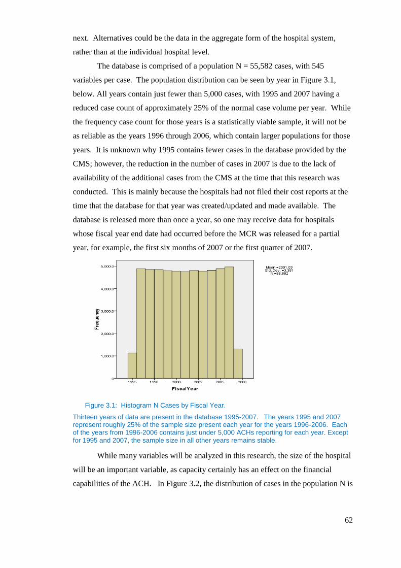
62
next. Alternatives could be the data in the aggregate form of the hospital system,
rather than at the individual hospital level.
The database is comprised of a population N = 55,582 cases, with 545
variables per case. The population distribution can be seen by year in Figure 3.1,
below. All years contain just fewer than 5,000 cases, with 1995 and 2007 having a
reduced case count of approximately 25% of the normal case volume per year. While
the frequency case count for those years is a statistically viable sample, it will not be
as reliable as the years 1996 through 2006, which contain larger populations for those
years. It is unknown why 1995 contains fewer cases in the database provided by the
CMS; however, the reduction in the number of cases in 2007 is due to the lack of
availability of the additional cases from the CMS at the time that this research was
conducted. This is mainly because the hospitals had not filed their cost reports at the
time that the database for that year was created/updated and made available. The
database is released more than once a year, so one may receive data for hospitals
whose fiscal year end date had occurred before the MCR was released for a partial
year, for example, the first six months of 2007 or the first quarter of 2007.
Figure 3.1: Histogram N Cases by Fiscal Year.
Thirteen years of data are present in the database 1995-2007. The years 1995 and 2007 represent roughly 25% of the sample size present each year for the years 1996-2006. Each of the years from 1996-2006 contains just under 5,000 ACHs reporting for each year. Except for 1995 and 2007, the sample size in all other years remains stable.
While many variables will be analyzed in this research, the size of the hospital
will be an important variable, as capacity certainly has an effect on the financial
capabilities of the ACH. In Figure 3.2, the distribution of cases in the population N is
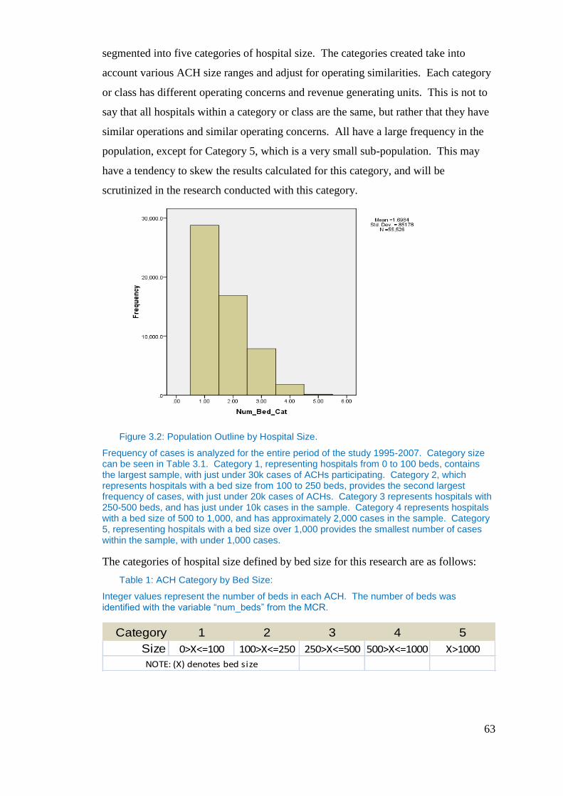
63
segmented into five categories of hospital size. The categories created take into
account various ACH size ranges and adjust for operating similarities. Each category
or class has different operating concerns and revenue generating units. This is not to
say that all hospitals within a category or class are the same, but rather that they have
similar operations and similar operating concerns. All have a large frequency in the
population, except for Category 5, which is a very small sub-population. This may
have a tendency to skew the results calculated for this category, and will be
scrutinized in the research conducted with this category.
Figure 3.2: Population Outline by Hospital Size.
Frequency of cases is analyzed for the entire period of the study 1995-2007. Category size can be seen in Table 3.1. Category 1, representing hospitals from 0 to 100 beds, contains the largest sample, with just under 30k cases of ACHs participating. Category 2, which represents hospitals with a bed size from 100 to 250 beds, provides the second largest frequency of cases, with just under 20k cases of ACHs. Category 3 represents hospitals with 250-500 beds, and has just under 10k cases in the sample. Category 4 represents hospitals with a bed size of 500 to 1,000, and has approximately 2,000 cases in the sample. Category 5, representing hospitals with a bed size over 1,000 provides the smallest number of cases within the sample, with under 1,000 cases.
The categories of hospital size defined by bed size for this research are as follows:
Table 1: ACH Category by Bed Size:
Integer values represent the number of beds in each ACH. The number of beds was identified with the variable “num_beds” from the MCR.
Category 1 2 3 4 5
Size 0>X<=100 100>X<=250 250>X<=500 500>X<=1000 X>1000
NOTE: (X) denotes bed size
64
3.3.3 Disadvantages of Data
The MCR has been criticized as unreliable, unaudited, lacking in detail, and
vaguely defined (Kane 2001). The greatest criticism is the lack of rigorous third-
party auditing of the information provided in the MCR. Most hospital-audited
financial statements are designed to provide information regarding an income
statement, a balance sheet, a statement of cash flows, changes in net assets, and to
give footnotes detailing the underlying nuances of transactions listed in the previous
statements. The MCR is lacking in comparison. Schedule G of the MCR does not
provide a statement of cash flows or footnotes. Largay and Stickney (1980), Sloan
(1996) and Kane and Magnus (2001) all suggest that the absence of cash flow
statements is a major deficiency. This makes an analysis of cash flows difficult, and
requires greater diligence in creating ratios that accurately reflect cash positions.
There are additional research questions that may be difficult to answer given
the information from within the MCR. Any questions regarding short-term operating
accountability or long-term financial stewardship of the firm are difficult to analyze
(Kane 2001). Kane (2001) provided a summary of key limitations with the MCRs
financial accounting elements: 1) major differences in the reported profits; 2)
inadequate balance sheet and income statement detail; and 3) inaccuracies related to
estimation of cash sources and uses. Cleverly (1992), Cleverly and Harvey (1990,
1992), and Bazzoli and Cleverly (1994) all call for greater, more complete financial
disclosure by hospitals than currently is supplied in the MCR. In addition, the data
does not distinguish between for-profit and non-for-profit, rural and urban hospitals.
While some effort is made in the current research to use standard industry
characterizations, for example in regards to rural and urban, a true delineation is not
possible. Therefore, comments within the research can only use the logic of these
characterizations. For instance, it is widely known that small hospitals are located in
areas with smaller populations and those urban areas or areas of smaller populations
are more likely to be rural in character. Likewise, larger hospitals are located in areas
with larger populations that are more likely located in large cities. A similar situation
presents itself for the for-profit and non-for-profit categories. While teaching
hospitals can be identified in the data and that it is known that most if not all teaching
hospitals are public non-for-profit, it remains a problem to be able to identify other
non-for-profit ACHs which may be in the data. For example, county run hospitals.

65
Therefore, it is not possible to break down variables and findings based on these
characteristics.
3.3.4 Data Preparation
While the CMS and other health researchers prepare the MCR for use, the
database itself is not entirely without error when the data is released. Errors and
omissions occur and must be cleansed or removed in order for research to be
conducted properly. An original N= 65,689 cases were available in the distributed
version of MCR by the CMS. After a quality test was performed on the data, it was
found that the MCR contained duplicate records. A match was performed, using the
fiscal year beginning date, fiscal year end date, hospital name, zip code, and state.
Approximately 92 cases were removed as a result of this process.
A cleanup of the hospital state and zip code was necessary. All zip codes were
verified via a third-party database of zip codes from the U.S. Postal Service. The state
was adjusted when it was different by observing previous years' reporting to
determine the actual state. This normally was verified by zip code. Hospitals not
identified via this methodology were researched individually on the Internet through
their websites, and the address was confirmed. No cases were removed as a result of
state or zip code errors.
The U.S. covers more than just the 50 U.S. states under Medicare and
Medicaid; U.S. territories also are included. This research was limited to the 48
contiguous states, plus Alaska and Hawaii; therefore, any cases that occurred outside
the 50 states were excluded from this research. These would include the U.S.
territories of Guam, the Virgin Islands, and Puerto Rico.
Hospitals report to the CMS throughout the year as their fiscal year end date is
reached; however, sub-year reporting was found in the MCR when reporting for less
than 363 days occurred. In this body of research, 363 days was used to reference a
full year’s data as opposed to 365 days, as the largest portion of cases within the
database reported a year to be 363 days or more. More than 363 days were allowed,
but a year was set as the minimum time frame allowed to be reported. Any
calculations that used days as the measurement were adjusted accordingly. Because
they reported less than 363 days, 5,235 cases were removed.

66
The mean for each variable, whether the mean was by itself or broken down
by year or size, were created with all of the cases for that particular year and size. Not
all of the hospitals were present throughout the longitudinal study. They may have
reported for a few years, stopped reporting, and started to report again later in the
study. No hospitals were excluded for this reason. The reasons for the lack of
reporting were unknown at the time that this research was conducted.
While the MCR provided basic balance sheets and income statement variables,
not all variables used in the creation of ratios used in this study were present in the
original database in its initial form, and some had to be created. Most ratio formulas
took the underlying variables directly from the MCR. If the variable was not
available, it was created by way of the other variables present. Evidence of this will
be visible in the definition of each ratio using data variable names. Null values were
prevalent for some variables within the MCR database. Where appropriate, a zero
value was used to replace the null or missing value. This was done so that ratios
could be calculated, and this included multiple variables that might not have been
reported as zero, but rather were left blank in the reporting. An example of this is
temporary investments. Many ACHs did not report a value for this field, which
ultimately is reflected in the MCR database as a null or missing value. Changing this
field to a zero did not change any ratios calculated with this field. This allowed many
cases that would have been excluded from the sample of the ratios because of missing
data to be included, thus increasing the sample size for the ratio.
All data provided in the MCR was input manually into the system at some
point. Errors in inputs led to the recording of extreme values for various variables.
These values were not removed from the population, but rather dealt with as extremes
and outliers when creating the subsamples for each ratio. Evidence of this will be
provided in the discussion on each ratio, where relevant.
Hospital type was considered in creation of the population to be studied.
While the MCR included many types of health facilities, general short-term, general
long-term, cancer, psychiatric, rehabilitation, religious non-medical, childrens, and
alchohol and drug, amongst others, only those that met characteristics of ACHs were
included. The variable of hospital type was limited to values of 1, 2, and 7. Hospitals
types are as follows: 1) General Short-Term; 2) General Long-Term; and 7)
Children’s Hospital. Removal of all other hospital types left a population of N =
67
55,582 cases. There were some records within the MCR data (38) that contained null
values in all variables, so they were removed permanently from the data.
3.4 Methodology
3.4.1 Introduction
The methodologies employed within this chapter provide a general view into
the data. All statistical calculations were done at a 95% confidence interval. The
population of each ratio was analyzed via box plot and stem and leaf to identify
extremes and outliers. Definitions of outlier and extremes are those defined by J.W.
Tukey (1977) to be three inter-quartile ranges below the twenty-fifth percentile or
above the seventy-fifth percentile. Outliers were removed from each population as
necessary to provide as close to a normalized distribution as possible.
Once a sample was created by removing outliers and extremes, a histogram of
the distribution of each was created. The removal of outliers improves the stability of
the variance of each year’s distribution and allows for a relatively homogeneous
statistic. This method improves the comparability of variables over time (Frecka
1983; Rees 1990)
The removal of outliers along with additional box plot and traditional
statistical descriptives were used to verify that a sample had been normalized. In all
samples, a mean and mode for that sample must be considered an acceptable value for
that particular ratio, with a small standard deviation and acceptable range. Both
skewness and kurtosis were used to verify that the character of the distribution is
acceptable, with limited skewness and limited kurtosis signifying normalization.
Each ratio’s statistical descriptives are presented pre- and post-removal of outliers and
can be seen in Table 3.2, below. For each ratio, the sample is normalized. Additional
details of the process are available in the appendix beginning with section 3.5.1.
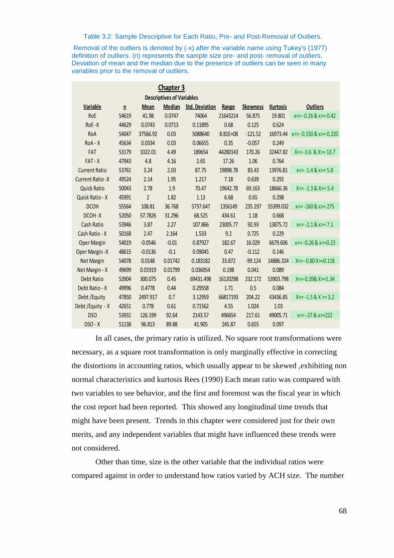
68
Table 3.2: Sample Descriptive for Each Ratio, Pre- and Post-Removal of Outliers.
Removal of the outliers is denoted by (-x) after the variable name using Tukey’s (1977) definition of outliers. (n) represents the sample size pre- and post- removal of outliers. Deviation of mean and the median due to the presence of outliers can be seen in many variables prior to the removal of outliers.
In all cases, the primary ratio is utilized. No square root transformations were
necessary, as a square root transformation is only marginally effective in correcting
the distortions in accounting ratios, which usually appear to be skewed ,exhibiting non
normal characteristics and kurtosis Rees (1990) Each mean ratio was compared with
two variables to see behavior, and the first and foremost was the fiscal year in which
the cost report had been reported. This showed any longitudinal time trends that
might have been present. Trends in this chapter were considered just for their own
merits, and any independent variables that might have influenced these trends were
not considered.
Other than time, size is the other variable that the individual ratios were
compared against in order to understand how ratios varied by ACH size. The number
Chapter 3Descriptives of Variables
Variable n Mean Median Std. Deviation Range Skewness Kurtosis Outliers
RoE 54619 41.98 0.0747 74064 21643214 56.875 19.801 x<= -0.26 & x>= 0.42
RoE -X 44629 0.0743 0.0713 0.11895 0.68 0.125 0.624
RoA 54047 37566.92 0.03 5088640 8.81E+08 -121.52 16973.44 x<= -0.150 & x>= 0.220
RoA - X 45634 0.0334 0.03 0.06655 0.35 -0.057 0.249
FAT 53179 1022.01 4.49 189654 44280143 170.26 32447.82 X<= -3.6 & X>= 13.7
FAT - X 47943 4.8 4.16 2.65 17.26 1.06 0.764
Current Ratio 53761 3.24 2.03 87.75 19898.78 83.43 13976.81 x<= -1.4 & x>= 5.8
Current Ratio -X 49524 2.14 1.95 1.217 7.18 0.639 0.292
Quick Ratio 50043 2.78 1.9 70.47 19642.78 69.163 18666.36 X<= -1.3 & X>= 5.4
Quick Ratio - X 45991 2 1.82 1.13 6.68 0.65 0.298
DCOH 55564 108.81 36.768 5737.647 1356149 235.197 55399.032 x<= -160 & x>= 275
DCOH -X 52050 57.7826 31.296 68.525 434.61 1.18 0.668
Cash Ratio 53946 3.87 2.27 107.866 23005.77 92.93 13875.72 x<= -2.1 & x>= 7.1
Cash Ratio - X 50168 2.47 2.164 1.533 9.2 0.725 0.229
Oper Margin 54019 -0.0546 -0.01 0.87927 182.67 16.029 6679.606 x<= -0.26 & x>=0.23
Oper Margin -X 48615 -0.0136 -0.1 0.09045 0.47 -0.112 0.146
Net Margin 54078 0.0148 0.01742 0.183182 33.872 -99.124 14886.324 X<= -0.80 X>=0.118
Net Margin - X 49699 0.01919 0.01799 0.036954 0.198 0.041 0.089
Debt Ratio 53904 300.075 0.45 69431.498 16120298 232.172 53903.798 X<=-0.39& X>=1.34
Debt Ratio - X 49996 0.4778 0.44 0.29558 1.71 0.5 0.084
Debt /Equity 47850 2497.917 0.7 3.12959 66817193 204.22 43436.85 X<= -1.5 & X >= 3.2
Debt /Equity - X 42651 0.778 0.61 0.71562 4.55 1.024 1.03
DSO 53931 126.199 92.64 2143.57 496654 217.61 49005.71 x<= -27 & x>=222
DSO - X 51138 96.813 89.88 41.905 245.87 0.655 0.097

69
of beds within a facility determined its size. The number of beds was signified by the
variable “num_beds” within the MCR (Medicare Cost Report) data itself (The
breakdown of these size categories is described in Section 3.4.2.). These interactions
were analyzed using tables and simple statistical descriptives of the comparison.
3.4.2 Ratios to Be Used in the Analysis
Using the research of Chen and Shimerda (1981) as a basis for choosing the
financial ratios to be studied, 12 ratios were chosen. While this study does not
attempt to separate financially-distressed firms from non-distressed firms, ratios that
gave clarity to condition and were more sensitive to indicating the distress of ACHs
were chosen. Ratios have been shown to be predictive of firm distress: “financially-
distressed firms can be separated from the non-failed firms in the year before the
declaration of bankruptcy at an accuracy rate of better than 90% by examining
financial ratios” (Altman 1968, in Chen & Shimerda 1981, p. 51).
Chen and Shimerda (1981), suggested that all of the financial ratios can be
assigned to one of the seven basic financial factors: return on investment, financial
leverage, capital turnover, cash position, liquidity (short-term), inventory turnover,
and receivables turnover. While some overlapping in ratios does occur as a result of
data peculiarities, ratios within this study address these seven basic financial factors.
A list of recommended financial ratios, descriptions, and equations for each can be
seen in Table 3.3.
Table 3.3: The Seven Basic Financial Factors and Recommended Ratios, by Chen and
Shimerda (1981), along with description and equation for each.
According to previous studies, these ratios have the highest loading score for
each of the seven financial factors. However, exactly which ratio should represent a
Ratio Type Description Equation
Profitability Return on Investment net income/total assets
Risk Leverage ratio long-term debt/equity
Efficiency Receivable turnover sales/ quick assets
capital turnover sales/ total assets
Inventory Turnover sales/ current assets
Liquidity Cash position cash / total assets
Liquidity ratio current assets / total assets
70
factor is still up for debate, as suggested by Chen and Shimerda (1981, p. 53): “An
acceptable theoretical foundation for the election of ratios for decision making has yet
to be found, and the scattered heterogeneous empirical evidence in the published
studies does not identify a complete set of useful ratios.” Chen and Shimerda (1981)
suggested that the financial ratios that capture most of the information for the
financial factor they represent should be chosen, so that a group of ratios will contain
more unique information.
To develop a predictive model of hospital closure using financial accounting
ratios, Wertheim and Lynn (1993) brought the selection of ratios in line with
healthcare in the U.S. and ACHs in their study. Their study compared 71 U.S.
hospitals using data taken from the two years preceding closure against data taken
from 71 operating hospitals with the same demographics between 1987 and 1995, and
it used Logit analysis. Univariate and multivariate tests were used to examine the
relationship between 21 financial ratios. They drew from the previous predictive
models of the LaJolla Management Corporation for the Bureau of Health Finance
(1981), the Farmers Home Administration checklist of financial ratios for assessing
rural hospitals (1983), Cleverly and Nilsen’s (1980) analysis of 14 closed hospitals in
New York, NY, Kwon et al.’s (1988) analysis of financial and operational
characteristics of Catholic hospitals, and Cleverly’s (1985) financial flexibility index,
or FFI. Wertheim and Lynn (1993) found, using the Lachenbruch Procedure, that 17
of the 21 ratios were significant indicators of hospital closure in the year prior to
closure, while only eight of the 21 were found to be significant in predicting hospital
closure in year two. The predictive ability of a ratio decreasing two years prior to
closure was found to be in line with prior research on the subject. “Rose and Giroux
(1984) indicate that as a firm approaches failure, financial factors leading to that
closure become more pronounced” (Wertheim & Lynn 1993, p.539).
Wertheim and Lynn (1993) narrowed down the set of seven financial factors
to four factors: 1) ratios representing leverage; 2) liquidity; 3) capital efficiency; and
4) asset availability. These ratios ultimately can provide significant information that
is useful in the prediction of hospital closures. Ratios for asset availability, capital
efficiency, and leverage were greater at predicting ACH closures than liquidity in a
multivariate model (Wertheim & Lynn, 1993). Total liabilities/total assets, total
revenues/total expenses, and total assets/bed days available were found to be
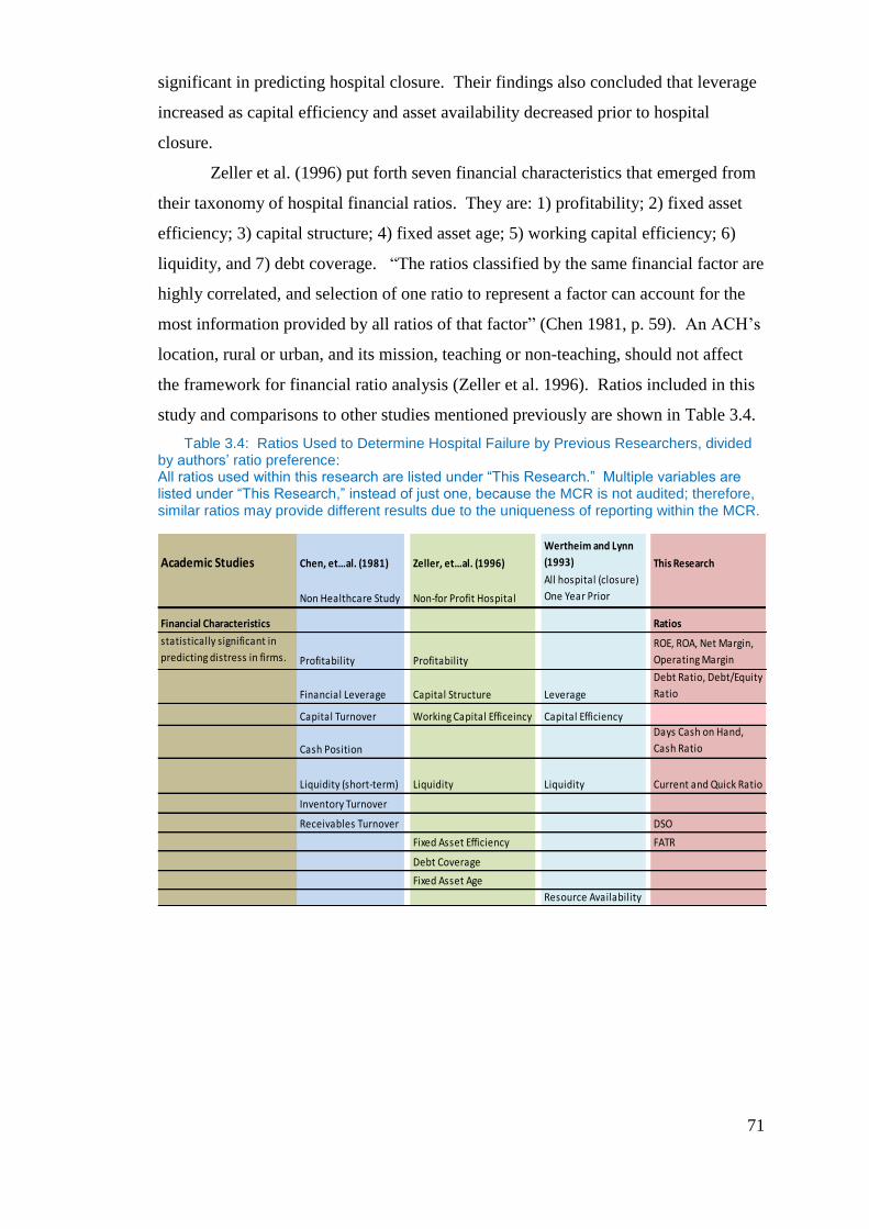
71
significant in predicting hospital closure. Their findings also concluded that leverage
increased as capital efficiency and asset availability decreased prior to hospital
closure.
Zeller et al. (1996) put forth seven financial characteristics that emerged from
their taxonomy of hospital financial ratios. They are: 1) profitability; 2) fixed asset
efficiency; 3) capital structure; 4) fixed asset age; 5) working capital efficiency; 6)
liquidity, and 7) debt coverage. “The ratios classified by the same financial factor are
highly correlated, and selection of one ratio to represent a factor can account for the
most information provided by all ratios of that factor” (Chen 1981, p. 59). An ACH’s
location, rural or urban, and its mission, teaching or non-teaching, should not affect
the framework for financial ratio analysis (Zeller et al. 1996). Ratios included in this
study and comparisons to other studies mentioned previously are shown in Table 3.4.
Table 3.4: Ratios Used to Determine Hospital Failure by Previous Researchers, divided by authors’ ratio preference: All ratios used within this research are listed under “This Research.” Multiple variables are listed under “This Research,” instead of just one, because the MCR is not audited; therefore, similar ratios may provide different results due to the uniqueness of reporting within the MCR.
Academic Studies Chen, et…al. (1981) Zeller, et…al. (1996)
Wertheim and Lynn
(1993) This Research
Non Healthcare Study Non-for Profit Hospital
All hospital (closure)
One Year Prior
Financial Characteristics Ratios
statistically significant in
predicting distress in firms. Profitability Profitability
ROE, ROA, Net Margin,
Operating Margin
Financial Leverage Capital Structure Leverage
Debt Ratio, Debt/Equity
Ratio
Capital Turnover Working Capital Efficeincy Capital Efficiency
Cash Position
Days Cash on Hand,
Cash Ratio
Liquidity (short-term) Liquidity Liquidity Current and Quick Ratio
Inventory Turnover
Receivables Turnover DSO
Fixed Asset Efficiency FATR
Debt Coverage
Fixed Asset Age
Resource Availability
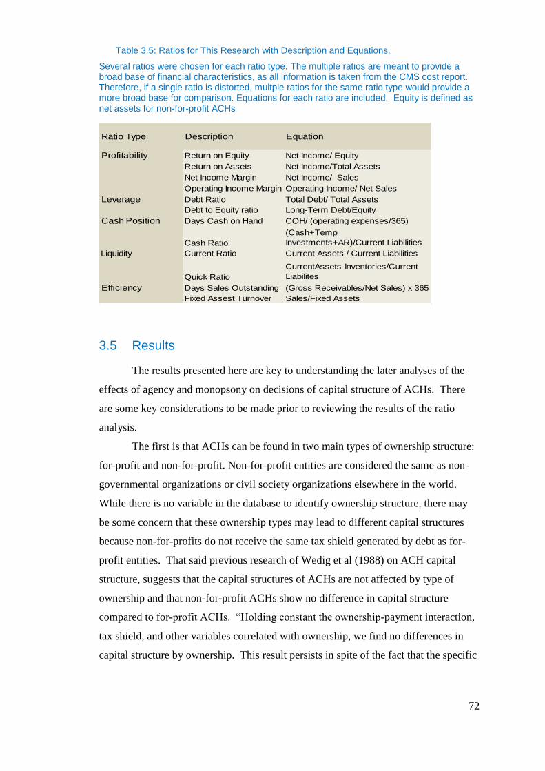
72
Table 3.5: Ratios for This Research with Description and Equations.
Several ratios were chosen for each ratio type. The multiple ratios are meant to provide a broad base of financial characteristics, as all information is taken from the CMS cost report. Therefore, if a single ratio is distorted, multple ratios for the same ratio type would provide a more broad base for comparison. Equations for each ratio are included. Equity is defined as net assets for non-for-profit ACHs
3.5 Results
The results presented here are key to understanding the later analyses of the
effects of agency and monopsony on decisions of capital structure of ACHs. There
are some key considerations to be made prior to reviewing the results of the ratio
analysis.
The first is that ACHs can be found in two main types of ownership structure:
for-profit and non-for-profit. Non-for-profit entities are considered the same as non-
governmental organizations or civil society organizations elsewhere in the world.
While there is no variable in the database to identify ownership structure, there may
be some concern that these ownership types may lead to different capital structures
because non-for-profits do not receive the same tax shield generated by debt as for-
profit entities. That said previous research of Wedig et al (1988) on ACH capital
structure, suggests that the capital structures of ACHs are not affected by type of
ownership and that non-for-profit ACHs show no difference in capital structure
compared to for-profit ACHs. “Holding constant the ownership-payment interaction,
tax shield, and other variables correlated with ownership, we find no differences in
capital structure by ownership. This result persists in spite of the fact that the specific
Ratio Type Description Equation
Profitability Return on Equity Net Income/ Equity
Return on Assets Net Income/Total Assets
Net Income Margin Net Income/ Sales
Operating Income Margin Operating Income/ Net Sales
Leverage Debt Ratio Total Debt/ Total Assets
Debt to Equity ratio Long-Term Debt/Equity
Cash Position Days Cash on Hand COH/ (operating expenses/365)
Cash Ratio
(Cash+Temp
Investments+AR)/Current Liabilities
Liquidity Current Ratio Current Assets / Current Liabilities
Quick Ratio
CurrentAssets-Inventories/Current
Liabilites
Efficiency Days Sales Outstanding (Gross Receivables/Net Sales) x 365
Fixed Assest Turnover Sales/Fixed Assets

73
motives for holding debt are quite different across ownership” (Wedig et al 1988,
p.37). This prior finding consequently supports our approach, which is to consider
leverage ratios across ACHs sizes and years without regard to ownership type.
The second and also a key concern is that an ACH’s location, rural or urban,
and its mission, teaching or non-teaching, may affect the framework for financial ratio
analysis. Research by Zeller et al. (1996) suggests that the composition of financial
ratios are not affected by these characteristics. This means that we are able to compare
and contrast the financial health of ACHs without regard to such features.
Third is that there may be some concern that certain ownership types of ACHs
may not recognize equity on the balance sheet in the same way. For-profit hospitals
issue shares to shareholders in the ACH, thus allowing for a measure of equity and
hence the creation of financial ratios mearsuring performance in comparison to the
equity investment. On the other hand, non-for-profit ACHs are generally owned by
the community or educational system which in turn is state or community owned.
Consequently there are potential difficulties in identifying a similar equity investment
category. However Conrad (1984) points out that non-for-profits can be measured
for equity performance as they still generate a return of equity capital due to
competition in the final product market for ACH services as well as in the capital
markets. Non-for-profits often keep retained earnings, fund balances or more recently
net assets, which are functionally equivalent to the equity investrment cateogry and
allow a definition of equity in financial ratios such as return on equity, and so on.
Researchers such as Long and Silver (1976), Long (1976) and Day (2008), argue for
the use of corporate finance principles in the non-for-profit healthcare sector by
suggesting that the same economic principles for investment decision making and
financial performance measurent apply between for-profit and non-for-profit
hospitals. Conrad (1984) furthers this approach in the light of his use of return on
equity taking the view that return on equity is an appropriate measure for non-for-
profit financial performance. Based on the above findings, in this research the equity
for non-for-profits is therefore defined as total assets minus total liabilities—rather
than net assets. This will is discussed later on in this chapter when examining the
financial performance of ACHs based on a ratio that includes equity in the
denominator,

74
That prior researchers have found no differences concerning location and
ownership type are important to this research as it reduces concerns that the observed
relationships that are found later on are driven by such characteristics. This means the
research can focus on the industry as a whole taking into account the entire population
of ACHs provided in the MCR during the timeframe of this study.
3.5.1 Profitability
The profitability of ACHs is included as a variable as prior researchers have
used it also and it is a component of free cash flows, which will be discussed later on.
However, problems with free cash flows should be indicative within the profitability
ratio. As profitability and free cash flow are linked, it is important to understand
changes in profitability over timeframe as free cash flow is a key variable to be
discussed later in empirical chapters where it used to provide evidence of agency and
monopsony. Fluctuations in profitability affect the ability of the ACH to obtain debt,
decisions of which are a main concern of this research.
ACH profitability is measured via four ratios: return on equity (ROE), return
on assets (ROA), net income margin (NIM), and operating income margin (OIM).
Equations for each profitability ratio are given in Table 3.4.3
Before discussing the profitability ratios, a proper understanding of net income
and operating income is needed as the MCR differs on the definition of operating
income from US GAAP, while net income does not. Operating income normally is
described as the amount of profit realized from a business's operations gross income
after taking out operating expenses, such as cost of goods sold (COGS), wages and
depreciation. This is often described as (EBIT) or earnings before interests and taxes.
The MCR differs in its definition of Operating Income in that the MCR refers to
operating income as the Net Income from Services to Patients (NISP). Therefore, in
this case the MCR definition does not start with gross income, but rather only
3 A detailed breakdown showing how each profitability ratio is created can be found in the
appendix within Section 3.5.1 together with a discussion of the underlying variables descriptive
statistics.

75
includes revenues generated at the ACH from services to patients. This definition of
Operating Income excludes Other Income obtained from sources such as Schedule G3
of the MCR. Other Income includes contributions, donations, income from
investments, revenues from television and phone rental, purchase discounts, rebates or
refunds, parking revenues, revenues from laundry, meals, rent, sales of medical or
surgical supplies, sale of drugs, medical record sales, tuition, and revenues from
vending. However, Net Income includes both the revenues defined as Operating
Income and revenues, which are defined as Other Income via the MCR. This
difference in the definition between net income and operating income is important as
will be shown further in section 3.5.1.
The data shows that ACHs have been affected financially over time. All
profitability ratios had their highest values in 1995 or 1996, and their lowest values in
1999, with the exception of the net income margin, which had its lowest value in
2002. Evidence of this can be followed in Table 3.5. All the measures of profitability
trend downward, as shown in Figure 3.4. While the trough of each profitability ratio
may vary, the worst performing periods correlate to the years 1998-2002, with the
exception of the operating margin, which had its worst performance beginning in
1996 as opposed to 1998. As shown in Table 3.5, net income margin, which had its
highest value in 1995 at 3.03%, is halved by the year 1999 at 1.5%, with a further
one-tenth of a percent decrease by 2002. By 1999, all ratios decreased significantly.
The return on equity (RoE) was down 39%, while the return on assets (RoA) was
down 48%. The Net Income Margin was down 50.5%, and the Operating Margin was
down by 289%.
All profitability ratios were positive, with the exception of the Operating
Margin, for which the mean is negative. While this may seem to contradict the
positive net margin, this is due to the MCR not following Generally Accepted
Accounting Principles (GAAP) reporting. The Operating Margin measured only the
margin that was derived directly from service to patients. This provided evidence
that ACHs on average were not profitable on services delivered to patients, and that
they must be profitable on other services delivered. This also helps explain the
magnitude in change over time between net income margin which decreased 50.5%
while the operating margin decreased 289%. The larger decrease in operating margin
can be directly be attributable to margin on patient services. This suggests that payors
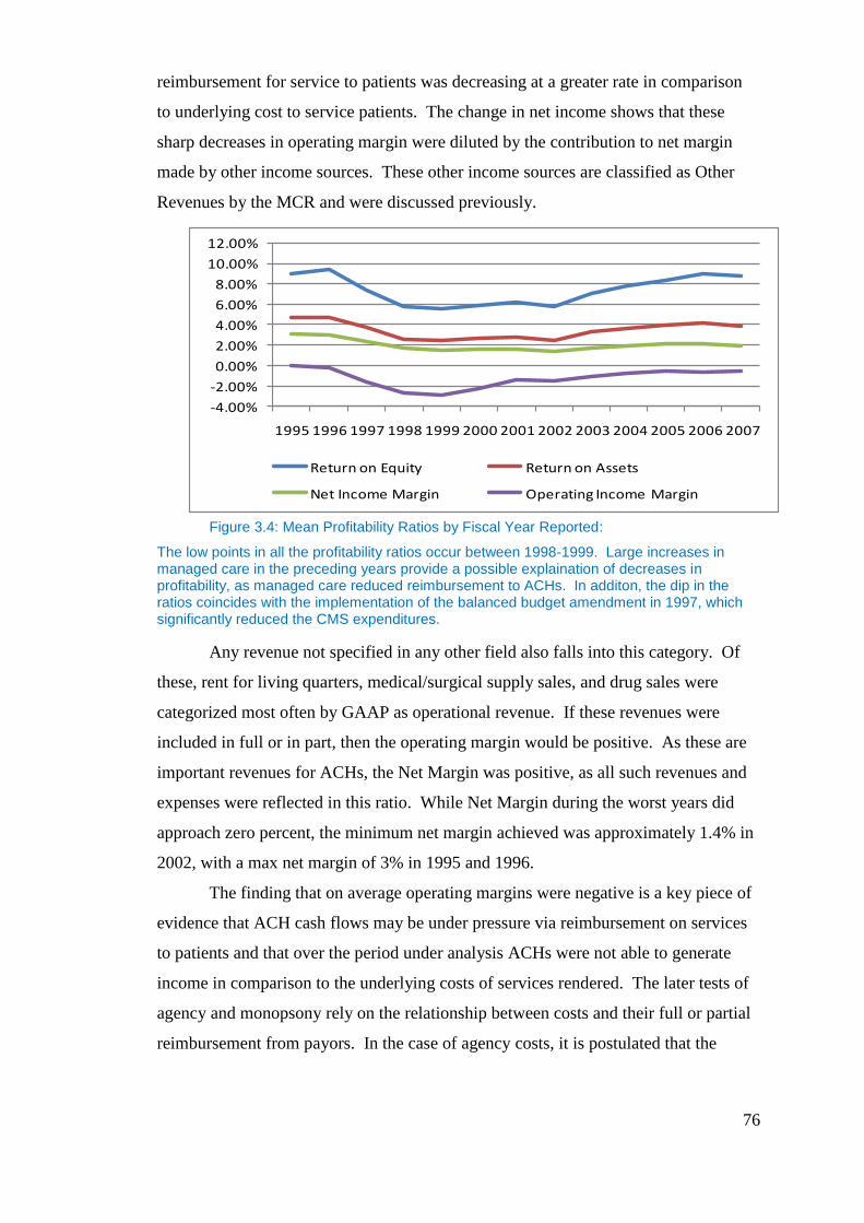
76
reimbursement for service to patients was decreasing at a greater rate in comparison
to underlying cost to service patients. The change in net income shows that these
sharp decreases in operating margin were diluted by the contribution to net margin
made by other income sources. These other income sources are classified as Other
Revenues by the MCR and were discussed previously.
Figure 3.4: Mean Profitability Ratios by Fiscal Year Reported:
The low points in all the profitability ratios occur between 1998-1999. Large increases in managed care in the preceding years provide a possible explaination of decreases in profitability, as managed care reduced reimbursement to ACHs. In additon, the dip in the ratios coincides with the implementation of the balanced budget amendment in 1997, which significantly reduced the CMS expenditures.
Any revenue not specified in any other field also falls into this category. Of
these, rent for living quarters, medical/surgical supply sales, and drug sales were
categorized most often by GAAP as operational revenue. If these revenues were
included in full or in part, then the operating margin would be positive. As these are
important revenues for ACHs, the Net Margin was positive, as all such revenues and
expenses were reflected in this ratio. While Net Margin during the worst years did
approach zero percent, the minimum net margin achieved was approximately 1.4% in
2002, with a max net margin of 3% in 1995 and 1996.
The finding that on average operating margins were negative is a key piece of
evidence that ACH cash flows may be under pressure via reimbursement on services
to patients and that over the period under analysis ACHs were not able to generate
income in comparison to the underlying costs of services rendered. The later tests of
agency and monopsony rely on the relationship between costs and their full or partial
reimbursement from payors. In the case of agency costs, it is postulated that the
-4.00%
-2.00%
0.00%
2.00%
4.00%
6.00%
8.00%
10.00%
12.00%
1995 1996 1997 1998 1999 2000 2001 2002 2003 2004 2005 2006 2007
Return on Equity Return on Assets
Net Income Margin Operating Income Margin
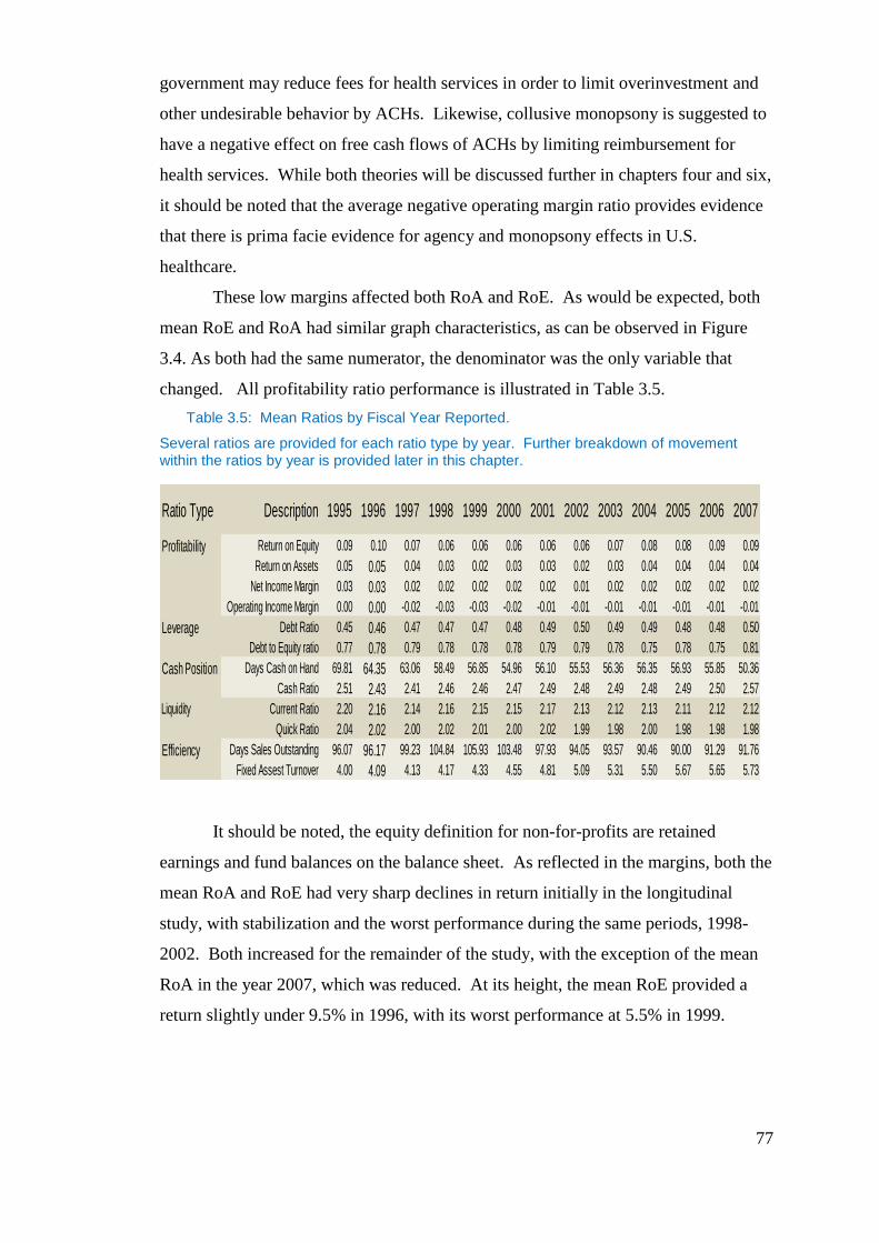
77
government may reduce fees for health services in order to limit overinvestment and
other undesirable behavior by ACHs. Likewise, collusive monopsony is suggested to
have a negative effect on free cash flows of ACHs by limiting reimbursement for
health services. While both theories will be discussed further in chapters four and six,
it should be noted that the average negative operating margin ratio provides evidence
that there is prima facie evidence for agency and monopsony effects in U.S.
healthcare.
These low margins affected both RoA and RoE. As would be expected, both
mean RoE and RoA had similar graph characteristics, as can be observed in Figure
3.4. As both had the same numerator, the denominator was the only variable that
changed. All profitability ratio performance is illustrated in Table 3.5.
Table 3.5: Mean Ratios by Fiscal Year Reported.
Several ratios are provided for each ratio type by year. Further breakdown of movement within the ratios by year is provided later in this chapter.
It should be noted, the equity definition for non-for-profits are retained
earnings and fund balances on the balance sheet. As reflected in the margins, both the
mean RoA and RoE had very sharp declines in return initially in the longitudinal
study, with stabilization and the worst performance during the same periods, 1998-
2002. Both increased for the remainder of the study, with the exception of the mean
RoA in the year 2007, which was reduced. At its height, the mean RoE provided a
return slightly under 9.5% in 1996, with its worst performance at 5.5% in 1999.
Ratio Type Description 1995 1996 1997 1998 1999 2000 2001 2002 2003 2004 2005 2006 2007
Profitability Return on Equity 0.09 0.10 0.07 0.06 0.06 0.06 0.06 0.06 0.07 0.08 0.08 0.09 0.09
Return on Assets 0.05 0.05 0.04 0.03 0.02 0.03 0.03 0.02 0.03 0.04 0.04 0.04 0.04
Net Income Margin 0.03 0.03 0.02 0.02 0.02 0.02 0.02 0.01 0.02 0.02 0.02 0.02 0.02
Operating Income Margin 0.00 0.00 -0.02 -0.03 -0.03 -0.02 -0.01 -0.01 -0.01 -0.01 -0.01 -0.01 -0.01
Leverage Debt Ratio 0.45 0.46 0.47 0.47 0.47 0.48 0.49 0.50 0.49 0.49 0.48 0.48 0.50
Debt to Equity ratio 0.77 0.78 0.79 0.78 0.78 0.78 0.79 0.79 0.78 0.75 0.78 0.75 0.81
Cash Position Days Cash on Hand 69.81 64.35 63.06 58.49 56.85 54.96 56.10 55.53 56.36 56.35 56.93 55.85 50.36
Cash Ratio 2.51 2.43 2.41 2.46 2.46 2.47 2.49 2.48 2.49 2.48 2.49 2.50 2.57
Liquidity Current Ratio 2.20 2.16 2.14 2.16 2.15 2.15 2.17 2.13 2.12 2.13 2.11 2.12 2.12
Quick Ratio 2.04 2.02 2.00 2.02 2.01 2.00 2.02 1.99 1.98 2.00 1.98 1.98 1.98
Efficiency Days Sales Outstanding 96.07 96.17 99.23 104.84 105.93 103.48 97.93 94.05 93.57 90.46 90.00 91.29 91.76
Fixed Assest Turnover 4.00 4.09 4.13 4.17 4.33 4.55 4.81 5.09 5.31 5.50 5.67 5.65 5.73
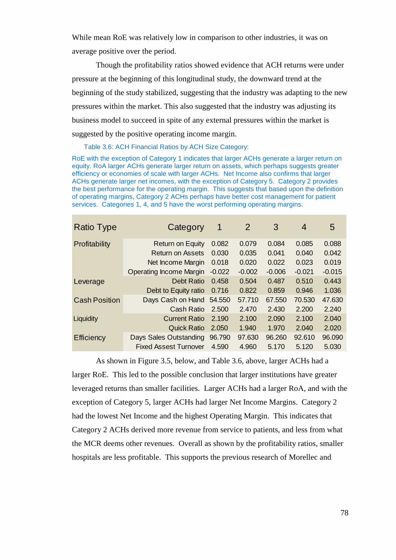
78
While mean RoE was relatively low in comparison to other industries, it was on
average positive over the period.
Though the profitability ratios showed evidence that ACH returns were under
pressure at the beginning of this longitudinal study, the downward trend at the
beginning of the study stabilized, suggesting that the industry was adapting to the new
pressures within the market. This also suggested that the industry was adjusting its
business model to succeed in spite of any external pressures within the market is
suggested by the positive operating income margin.
Table 3.6: ACH Financial Ratios by ACH Size Category:
RoE with the exception of Category 1 indicates that larger ACHs generate a larger return on equity. RoA larger ACHs generate larger return on assets, which perhaps suggests greater efficiency or economies of scale with larger ACHs. Net Income also confirms that larger ACHs generate larger net incomes, with the exception of Category 5. Category 2 provides the best performance for the operating margin. This suggests that based upon the definition of operating margins, Category 2 ACHs perhaps have better cost management for patient services. Categories 1, 4, and 5 have the worst performing operating margins.
As shown in Figure 3.5, below, and Table 3.6, above, larger ACHs had a
larger RoE. This led to the possible conclusion that larger institutions have greater
leveraged returns than smaller facilities. Larger ACHs had a larger RoA, and with the
exception of Category 5, larger ACHs had larger Net Income Margins. Category 2
had the lowest Net Income and the highest Operating Margin. This indicates that
Category 2 ACHs derived more revenue from service to patients, and less from what
the MCR deems other revenues. Overall as shown by the profitability ratios, smaller
hospitals are less profitable. This supports the previous research of Morellec and
Ratio Type Category 1 2 3 4 5
Profitability Return on Equity 0.082 0.079 0.084 0.085 0.088
Return on Assets 0.030 0.035 0.041 0.040 0.042
Net Income Margin 0.018 0.020 0.022 0.023 0.019
Operating Income Margin -0.022 -0.002 -0.006 -0.021 -0.015
Leverage Debt Ratio 0.458 0.504 0.487 0.510 0.443
Debt to Equity ratio 0.716 0.822 0.859 0.946 1.036
Cash Position Days Cash on Hand 54.550 57.710 67.550 70.530 47.630
Cash Ratio 2.500 2.470 2.430 2.200 2.240
Liquidity Current Ratio 2.190 2.100 2.090 2.100 2.040
Quick Ratio 2.050 1.940 1.970 2.040 2.020
Efficiency Days Sales Outstanding 96.790 97.630 96.260 92.610 96.090
Fixed Assest Turnover 4.590 4.960 5.170 5.120 5.030
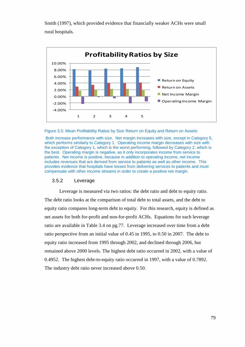
79
Smith (1997), which provided evidence that financially weaker ACHs were small
rural hospitals.
Figure 3.5: Mean Profitability Ratios by Size Return on Equity and Return on Assets:
Both increase performance with size. Net margin increases with size, except in Category 5, which performs similarly to Category 1. Operating income margin decreases with size with the exception of Category 1, which is the worst performing, followed by Category 2, which is the best. Operating margin is negative, as it only incorporates income from service to patients. Net income is positive, because in addition to operating income, net income includes revenues that are derived from service to patients as well as other income. This provides evidence that hospitals have losses from delivering services to patients and must compensate with other income streams in order to create a positive net margin.
3.5.2 Leverage
Leverage is measured via two ratios: the debt ratio and debt to equity ratio.
The debt ratio looks at the comparison of total debt to total assets, and the debt to
equity ratio compares long-term debt to equity. For this research, equity is defined as
net assets for both for-profit and non-for-profit ACHs. Equations for each leverage
ratio are available in Table 3.4 on pg.77. Leverage increased over time from a debt
ratio perspective from an initial value of 0.45 in 1995, to 0.50 in 2007. The debt to
equity ratio increased from 1995 through 2002, and declined through 2006, but
remained above 2000 levels. The highest debt ratio occurred in 2002, with a value of
0.4952. The highest debt-to-equity ratio occurred in 1997, with a value of 0.7892.
The industry debt ratio never increased above 0.50.
-4.00%
-2.00%
0.00%
2.00%
4.00%
6.00%
8.00%
10.00%
1 2 3 4 5
Profitability Ratios by Size
Return on Equity
Return on Assets
Net Income Margin
Operating Income Margin
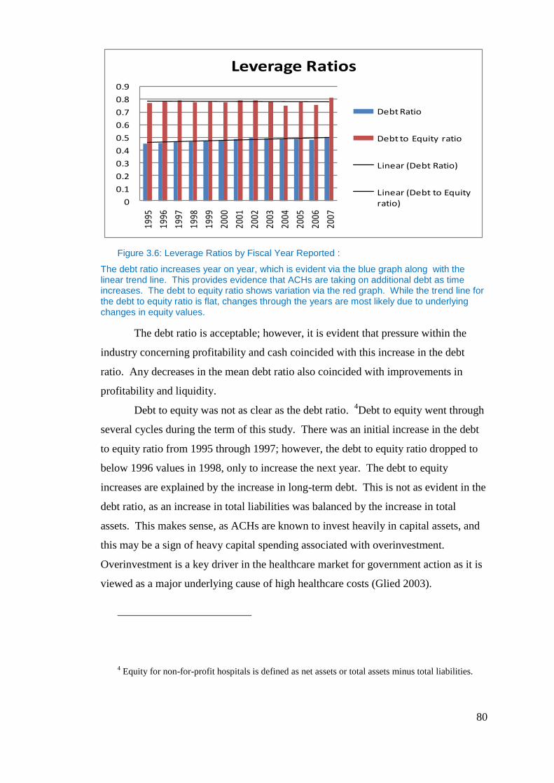
80
Figure 3.6: Leverage Ratios by Fiscal Year Reported :
The debt ratio increases year on year, which is evident via the blue graph along with the linear trend line. This provides evidence that ACHs are taking on additional debt as time increases. The debt to equity ratio shows variation via the red graph. While the trend line for the debt to equity ratio is flat, changes through the years are most likely due to underlying changes in equity values.
The debt ratio is acceptable; however, it is evident that pressure within the
industry concerning profitability and cash coincided with this increase in the debt
ratio. Any decreases in the mean debt ratio also coincided with improvements in
profitability and liquidity.
Debt to equity was not as clear as the debt ratio. 4Debt to equity went through
several cycles during the term of this study. There was an initial increase in the debt
to equity ratio from 1995 through 1997; however, the debt to equity ratio dropped to
below 1996 values in 1998, only to increase the next year. The debt to equity
increases are explained by the increase in long-term debt. This is not as evident in the
debt ratio, as an increase in total liabilities was balanced by the increase in total
assets. This makes sense, as ACHs are known to invest heavily in capital assets, and
this may be a sign of heavy capital spending associated with overinvestment.
Overinvestment is a key driver in the healthcare market for government action as it is
viewed as a major underlying cause of high healthcare costs (Glied 2003).
4 Equity for non-for-profit hospitals is defined as net assets or total assets minus total liabilities.
0
0.1
0.2
0.3
0.4
0.5
0.6
0.7
0.8
0.9
1995
1996
1997
1998
1999
2000
2001
2002
2003
2004
2005
2006
2007
Leverage Ratios
Debt Ratio
Debt to Equity ratio
Linear (Debt Ratio)
Linear (Debt to Equity ratio)
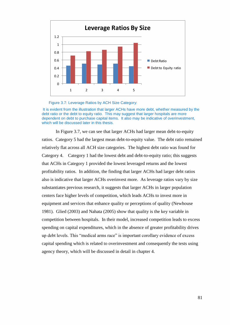
81
Figure 3.7: Leverage Ratios by ACH Size Category:
It is evident from the illustration that larger ACHs have more debt, whether measured by the debt ratio or the debt to equity ratio. This may suggest that larger hospitals are more dependent on debt to purchase capital items. It also may be indicative of overinvestment, which will be discussed later in this thesis.
In Figure 3.7, we can see that larger ACHs had larger mean debt-to-equity
ratios. Category 5 had the largest mean debt-to-equity value. The debt ratio remained
relatively flat across all ACH size categories. The highest debt ratio was found for
Category 4. Category 1 had the lowest debt and debt-to-equity ratio; this suggests
that ACHs in Category 1 provided the lowest leveraged returns and the lowest
profitability ratios. In addition, the finding that larger ACHs had larger debt ratios
also is indicative that larger ACHs overinvest more. As leverage ratios vary by size
substantiates previous research, it suggests that larger ACHs in larger population
centers face higher levels of competition, which leads ACHs to invest more in
equipment and services that enhance quality or perceptions of quality (Newhouse
1981). Glied (2003) and Nahata (2005) show that quality is the key variable in
competition between hospitals. In their model, increased competition leads to excess
spending on capital expenditures, which in the absence of greater profitability drives
up debt levels. This “medical arms race” is important corollary evidence of excess
capital spending which is related to overinvestment and consequently the tests using
agency theory, which will be discussed in detail in chapter 4.
0
0.2
0.4
0.6
0.8
1
1.2
1 2 3 4 5
Leverage Ratios By Size
Debt Ratio
Debt to Equity ratio
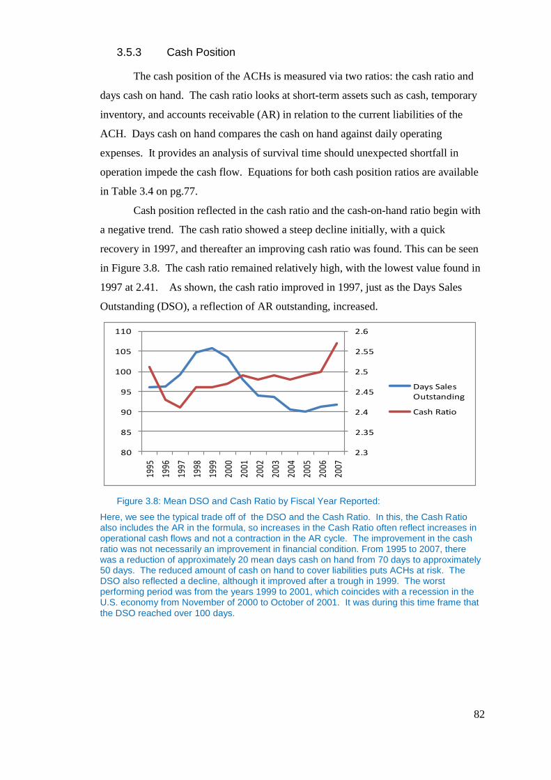
82
3.5.3 Cash Position
The cash position of the ACHs is measured via two ratios: the cash ratio and
days cash on hand. The cash ratio looks at short-term assets such as cash, temporary
inventory, and accounts receivable (AR) in relation to the current liabilities of the
ACH. Days cash on hand compares the cash on hand against daily operating
expenses. It provides an analysis of survival time should unexpected shortfall in
operation impede the cash flow. Equations for both cash position ratios are available
in Table 3.4 on pg.77.
Cash position reflected in the cash ratio and the cash-on-hand ratio begin with
a negative trend. The cash ratio showed a steep decline initially, with a quick
recovery in 1997, and thereafter an improving cash ratio was found. This can be seen
in Figure 3.8. The cash ratio remained relatively high, with the lowest value found in
1997 at 2.41. As shown, the cash ratio improved in 1997, just as the Days Sales
Outstanding (DSO), a reflection of AR outstanding, increased.
Figure 3.8: Mean DSO and Cash Ratio by Fiscal Year Reported:
Here, we see the typical trade off of the DSO and the Cash Ratio. In this, the Cash Ratio also includes the AR in the formula, so increases in the Cash Ratio often reflect increases in operational cash flows and not a contraction in the AR cycle. The improvement in the cash ratio was not necessarily an improvement in financial condition. From 1995 to 2007, there was a reduction of approximately 20 mean days cash on hand from 70 days to approximately 50 days. The reduced amount of cash on hand to cover liabilities puts ACHs at risk. The DSO also reflected a decline, although it improved after a trough in 1999. The worst performing period was from the years 1999 to 2001, which coincides with a recession in the U.S. economy from November of 2000 to October of 2001. It was during this time frame that the DSO reached over 100 days.
2.3
2.35
2.4
2.45
2.5
2.55
2.6
80
85
90
95
100
105
110
1995
1996
1997
1998
1999
2000
2001
2002
2003
2004
2005
2006
2007
Days Sales Outstanding
Cash Ratio
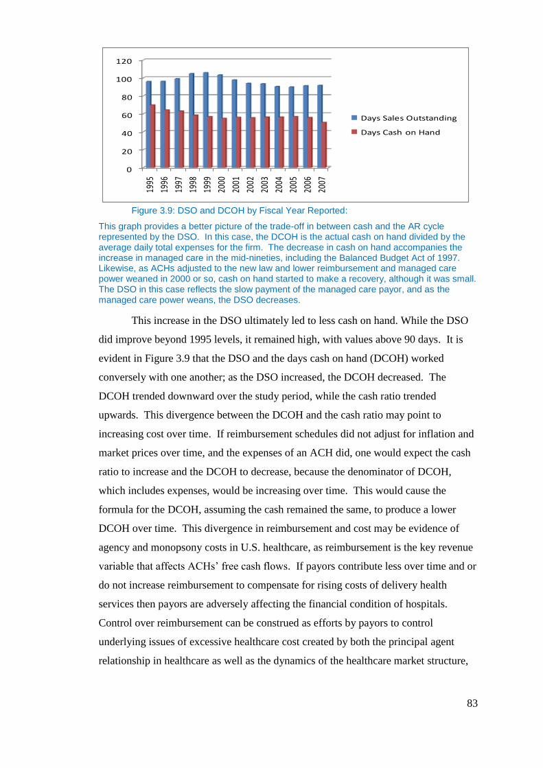
83
Figure 3.9: DSO and DCOH by Fiscal Year Reported:
This graph provides a better picture of the trade-off in between cash and the AR cycle represented by the DSO. In this case, the DCOH is the actual cash on hand divided by the average daily total expenses for the firm. The decrease in cash on hand accompanies the increase in managed care in the mid-nineties, including the Balanced Budget Act of 1997. Likewise, as ACHs adjusted to the new law and lower reimbursement and managed care power weaned in 2000 or so, cash on hand started to make a recovery, although it was small. The DSO in this case reflects the slow payment of the managed care payor, and as the managed care power weans, the DSO decreases.
This increase in the DSO ultimately led to less cash on hand. While the DSO
did improve beyond 1995 levels, it remained high, with values above 90 days. It is
evident in Figure 3.9 that the DSO and the days cash on hand (DCOH) worked
conversely with one another; as the DSO increased, the DCOH decreased. The
DCOH trended downward over the study period, while the cash ratio trended
upwards. This divergence between the DCOH and the cash ratio may point to
increasing cost over time. If reimbursement schedules did not adjust for inflation and
market prices over time, and the expenses of an ACH did, one would expect the cash
ratio to increase and the DCOH to decrease, because the denominator of DCOH,
which includes expenses, would be increasing over time. This would cause the
formula for the DCOH, assuming the cash remained the same, to produce a lower
DCOH over time. This divergence in reimbursement and cost may be evidence of
agency and monopsony costs in U.S. healthcare, as reimbursement is the key revenue
variable that affects ACHs’ free cash flows. If payors contribute less over time and or
do not increase reimbursement to compensate for rising costs of delivery health
services then payors are adversely affecting the financial condition of hospitals.
Control over reimbursement can be construed as efforts by payors to control
underlying issues of excessive healthcare cost created by both the principal agent
relationship in healthcare as well as the dynamics of the healthcare market structure,
0
20
40
60
80
100
120
1995
1996
1997
1998
1999
2000
2001
2002
2003
2004
2005
2006
2007
Days Sales Outstanding
Days Cash on Hand
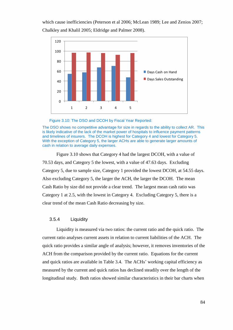
84
which cause inefficiencies (Peterson et al 2006; McLean 1989; Lee and Zenios 2007;
Chalkley and Khalil 2005; Eldridge and Palmer 2008).
Figure 3.10: The DSO and DCOH by Fiscal Year Reported:
The DSO shows no competitive advantage for size in regards to the ability to collect AR. This is likely indicative of the lack of the market power of hospitals to influence payment patterns and timelines of insurers. The DCOH is highest for Category 4 and lowest for Category 5. With the exception of Category 5, the larger ACHs are able to generate larger amounts of cash in relation to average daily expenses.
Figure 3.10 shows that Category 4 had the largest DCOH, with a value of
70.53 days, and Category 5 the lowest, with a value of 47.63 days. Excluding
Category 5, due to sample size, Category 1 provided the lowest DCOH, at 54.55 days.
Also excluding Category 5, the larger the ACH, the larger the DCOH. The mean
Cash Ratio by size did not provide a clear trend. The largest mean cash ratio was
Category 1 at 2.5, with the lowest in Category 4. Excluding Category 5, there is a
clear trend of the mean Cash Ratio decreasing by size.
3.5.4 Liquidity
Liquidity is measured via two ratios: the current ratio and the quick ratio. The
current ratio analyses current assets in relation to current liabilities of the ACH. The
quick ratio provides a similar angle of analysis; however, it removes inventories of the
ACH from the comparison provided by the current ratio. Equations for the current
and quick ratios are available in Table 3.4. The ACHs’ working capital efficiency as
measured by the current and quick ratios has declined steadily over the length of the
longitudinal study. Both ratios showed similar characteristics in their bar charts when
0
20
40
60
80
100
120
1 2 3 4 5
Days Cash on Hand
Days Sales Outstanding
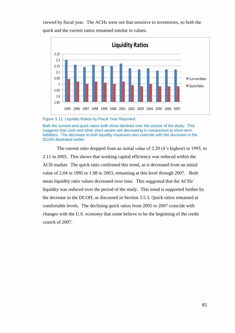
85
viewed by fiscal year. The ACHs were not that sensitive to inventories, so both the
quick and the current ratios remained similar in values.
Figure 3.11: Liquidity Ratios by Fiscal Year Reported:
Both the current and quick ratios both show declines over the course of the study. This suggests that cash and other short assets are decreasing in comparison to short-term liabilities. The decrease in both liquidity measures also coincide with the decrease in the DCOH illustrated earlier.
The current ratio dropped from an initial value of 2.20 (it’s highest) in 1995, to
2.11 in 2005. This shows that working capital efficiency was reduced within the
ACH market. The quick ratio confirmed this trend, as it decreased from an initial
value of 2.04 in 1995 to 1.98 in 2003, remaining at this level through 2007. Both
mean liquidity ratio values decreased over time. This suggested that the ACHs’
liquidity was reduced over the period of the study. This trend is supported further by
the decrease in the DCOH, as discussed in Section 3.5.3. Quick ratios remained at
comfortable levels. The declining quick ratios from 2005 to 2007 coincide with
changes with the U.S. economy that some believe to be the beginning of the credit
crunch of 2007.
1.85
1.9
1.95
2
2.05
2.1
2.15
2.2
2.25
1995 1996 1997 1998 1999 2000 2001 2002 2003 2004 2005 2006 2007
Liquidity Ratios
Current Ratio
Quick Ratio
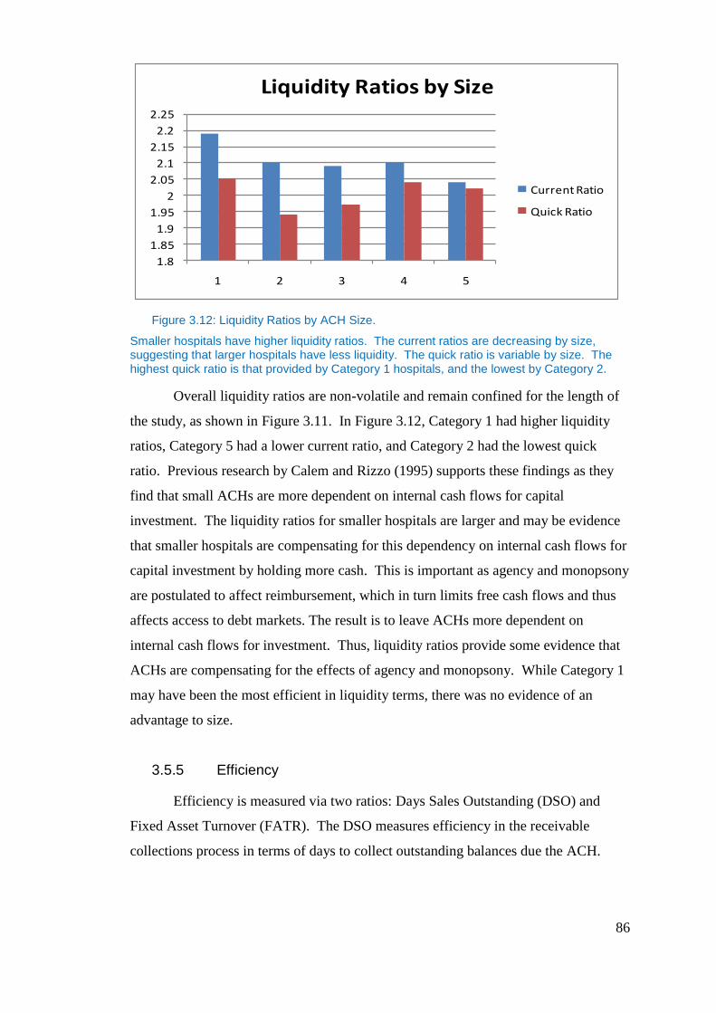
86
Figure 3.12: Liquidity Ratios by ACH Size.
Smaller hospitals have higher liquidity ratios. The current ratios are decreasing by size, suggesting that larger hospitals have less liquidity. The quick ratio is variable by size. The highest quick ratio is that provided by Category 1 hospitals, and the lowest by Category 2.
Overall liquidity ratios are non-volatile and remain confined for the length of
the study, as shown in Figure 3.11. In Figure 3.12, Category 1 had higher liquidity
ratios, Category 5 had a lower current ratio, and Category 2 had the lowest quick
ratio. Previous research by Calem and Rizzo (1995) supports these findings as they
find that small ACHs are more dependent on internal cash flows for capital
investment. The liquidity ratios for smaller hospitals are larger and may be evidence
that smaller hospitals are compensating for this dependency on internal cash flows for
capital investment by holding more cash. This is important as agency and monopsony
are postulated to affect reimbursement, which in turn limits free cash flows and thus
affects access to debt markets. The result is to leave ACHs more dependent on
internal cash flows for investment. Thus, liquidity ratios provide some evidence that
ACHs are compensating for the effects of agency and monopsony. While Category 1
may have been the most efficient in liquidity terms, there was no evidence of an
advantage to size.
3.5.5 Efficiency
Efficiency is measured via two ratios: Days Sales Outstanding (DSO) and
Fixed Asset Turnover (FATR). The DSO measures efficiency in the receivable
collections process in terms of days to collect outstanding balances due the ACH.
1.8
1.85
1.9
1.95
2
2.05
2.1
2.15
2.2
2.25
1 2 3 4 5
Liquidity Ratios by Size
Current Ratio
Quick Ratio
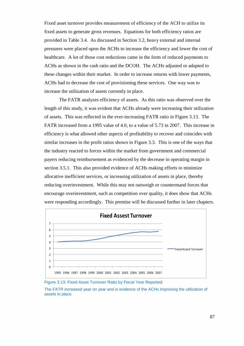
87
Fixed asset turnover provides measurement of efficiency of the ACH to utilize its
fixed assets to generate gross revenues. Equations for both efficiency ratios are
provided in Table 3.4. As discussed in Section 3.2, heavy external and internal
pressures were placed upon the ACHs to increase the efficiency and lower the cost of
healthcare. A lot of those cost reductions came in the form of reduced payments to
ACHs as shown in the cash ratio and the DCOH. The ACHs adjusted or adapted to
these changes within their market. In order to increase returns with lower payments,
ACHs had to decrease the cost of provisioning these services. One way was to
increase the utilization of assets currently in place.
The FATR analyzes efficiency of assets. As this ratio was observed over the
length of this study, it was evident that ACHs already were increasing their utilization
of assets. This was reflected in the ever-increasing FATR ratio in Figure 3.13. The
FATR increased from a 1995 value of 4.0, to a value of 5.73 in 2007. This increase in
efficiency is what allowed other aspects of profitability to recover and coincides with
similar increases in the profit ratios shown in Figure 3.3. This is one of the ways that
the industry reacted to forces within the market from government and commercial
payers reducing reimbursement as evidenced by the decrease in operating margin in
section 3.5.1. This also provided evidence of ACHs making efforts to minimize
allocative inefficient services, or increasing utilization of assets in place, thereby
reducing overinvestment. While this may not outweigh or countermand forces that
encourage overinvestment, such as competition over quality, it does show that ACHs
were responding accordingly. This premise will be discussed further in later chapters.
Figure 3.13: Fixed Asset Turnover Ratio by Fiscal Year Reported:
The FATR increased year on year and is evidence of the ACHs improving the utilization of assets in place.
0
1
2
3
4
5
6
7
1995 1996 1997 1998 1999 2000 2001 2002 2003 2004 2005 2006 2007
Fixed Assest Turnover
Fixed Assest Turnover
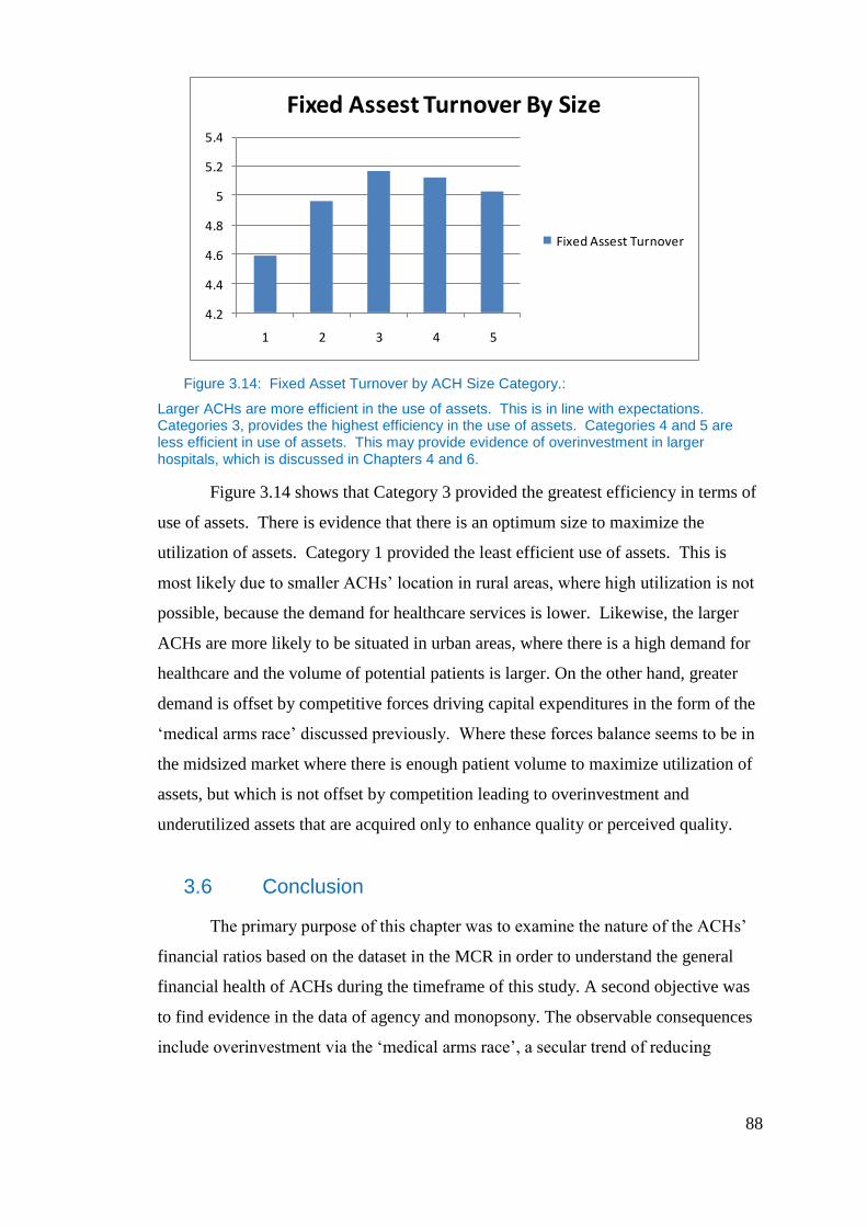
88
Figure 3.14: Fixed Asset Turnover by ACH Size Category.:
Larger ACHs are more efficient in the use of assets. This is in line with expectations. Categories 3, provides the highest efficiency in the use of assets. Categories 4 and 5 are less efficient in use of assets. This may provide evidence of overinvestment in larger hospitals, which is discussed in Chapters 4 and 6.
Figure 3.14 shows that Category 3 provided the greatest efficiency in terms of
use of assets. There is evidence that there is an optimum size to maximize the
utilization of assets. Category 1 provided the least efficient use of assets. This is
most likely due to smaller ACHs’ location in rural areas, where high utilization is not
possible, because the demand for healthcare services is lower. Likewise, the larger
ACHs are more likely to be situated in urban areas, where there is a high demand for
healthcare and the volume of potential patients is larger. On the other hand, greater
demand is offset by competitive forces driving capital expenditures in the form of the
‘medical arms race’ discussed previously. Where these forces balance seems to be in
the midsized market where there is enough patient volume to maximize utilization of
assets, but which is not offset by competition leading to overinvestment and
underutilized assets that are acquired only to enhance quality or perceived quality.
3.6 Conclusion
The primary purpose of this chapter was to examine the nature of the ACHs’
financial ratios based on the dataset in the MCR in order to understand the general
financial health of ACHs during the timeframe of this study. A second objective was
to find evidence in the data of agency and monopsony. The observable consequences
include overinvestment via the ‘medical arms race’, a secular trend of reducing
4.2
4.4
4.6
4.8
5
5.2
5.4
1 2 3 4 5
Fixed Assest Turnover By Size
Fixed Assest Turnover
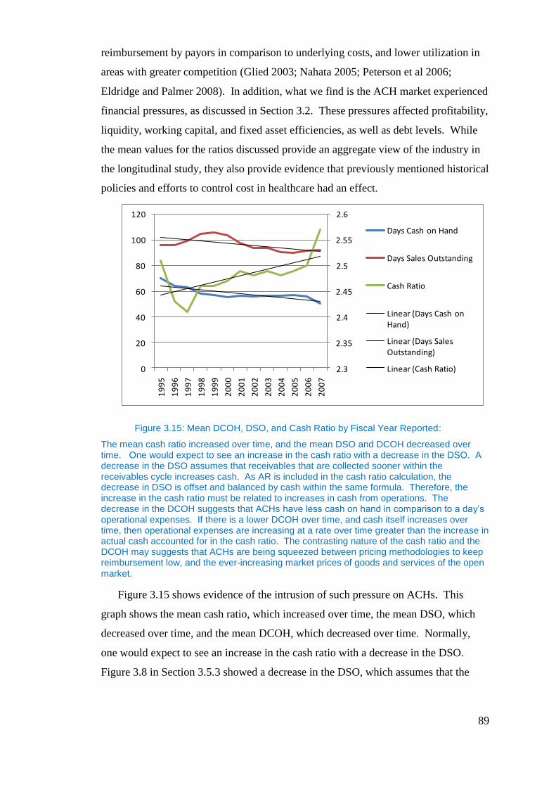
89
reimbursement by payors in comparison to underlying costs, and lower utilization in
areas with greater competition (Glied 2003; Nahata 2005; Peterson et al 2006;
Eldridge and Palmer 2008). In addition, what we find is the ACH market experienced
financial pressures, as discussed in Section 3.2. These pressures affected profitability,
liquidity, working capital, and fixed asset efficiencies, as well as debt levels. While
the mean values for the ratios discussed provide an aggregate view of the industry in
the longitudinal study, they also provide evidence that previously mentioned historical
policies and efforts to control cost in healthcare had an effect.
Figure 3.15: Mean DCOH, DSO, and Cash Ratio by Fiscal Year Reported:
The mean cash ratio increased over time, and the mean DSO and DCOH decreased over time. One would expect to see an increase in the cash ratio with a decrease in the DSO. A decrease in the DSO assumes that receivables that are collected sooner within the receivables cycle increases cash. As AR is included in the cash ratio calculation, the decrease in DSO is offset and balanced by cash within the same formula. Therefore, the increase in the cash ratio must be related to increases in cash from operations. The decrease in the DCOH suggests that ACHs have less cash on hand in comparison to a day’s operational expenses. If there is a lower DCOH over time, and cash itself increases over time, then operational expenses are increasing at a rate over time greater than the increase in actual cash accounted for in the cash ratio. The contrasting nature of the cash ratio and the DCOH may suggests that ACHs are being squeezed between pricing methodologies to keep reimbursement low, and the ever-increasing market prices of goods and services of the open market.
Figure 3.15 shows evidence of the intrusion of such pressure on ACHs. This
graph shows the mean cash ratio, which increased over time, the mean DSO, which
decreased over time, and the mean DCOH, which decreased over time. Normally,
one would expect to see an increase in the cash ratio with a decrease in the DSO.
Figure 3.8 in Section 3.5.3 showed a decrease in the DSO, which assumes that the
2.3
2.35
2.4
2.45
2.5
2.55
2.6
0
20
40
60
80
100
120
19
95
19
96
19
97
19
98
19
99
20
00
20
01
20
02
20
03
20
04
20
05
20
06
20
07
Days Cash on Hand
Days Sales Outstanding
Cash Ratio
Linear (Days Cash on Hand)
Linear (Days Sales Outstanding)
Linear (Cash Ratio)

90
receivables collected sooner within the receivables cycle increases cash. As AR is
included in the cash ratio calculation, the decrease in DSO was offset by and balanced
by cash within the same formula. Therefore, the increase in the cash ratio uncovered
by this study must be related to increases in cash from operations.
When observing the previous phenomena with the DCOH over the same
period, there is evidence of market pricing pressures upon ACHs. The decrease in the
DCOH suggests that ACHs have less cash on hand in comparison to a day’s
operational expenses. Therefore, if there is a lower DCOH over time, and it is known
that cash itself increases over time, then the only explanation for the decrease in the
day’s cash on hand is that operational expenses are increasing at a rate over time
greater than the increase in actual cash accounted for in the cash ratio. Therefore, this
may suggest that ACHs are being squeezed between pricing strategies by payors to
keep reimbursement for healthcare services low, and the ever-increasing market
prices of goods and services purchased by ACHs on the open market, as provided by
evidence of the contrasting nature of the cash ratio and the DCOH.
If in addition we examine profitability ratios, which all show a decreasing
trend over the period studied, we can find additional evidence of the trends seen in the
divergence of the DCOH and the cash ratio. This provides additional evidence that
ACH reimbursement for services over this period was not covering the costs of the
services rendered. This effect is especially noticeable in ACHs’ operating margin as
this is a good indicator of margin accrued from services to patients. While not
conclusive, this may be evidence for agency and monopsony effects as both are
postulated to affect free cash flows via reimbursement for health services.
Overinvestment is a key component of the agency argument put forth in this
thesis. As Newhouse (1981), Glied (2003) and Nahata (2005) find ACHs may be
overinvesting in projects that have low or negative net present values, driven by the
need to compete on quality. Supporting this argument, Wang (1999) finds that firms
with higher levels of competition overinvest more. We see evidence of this in Section
3.5.2 where larger ACHs have higher debt ratios, which suggests more capital
spending by larger hospitals in highly competitive geographic areas. Evidence of
overinvestment provides a basis for the presence of agency cost discussed in Chapter
4.
91
The liquidity ratios discussed in Section 3.5.4 provide additional evidence that
smaller ACHs were more liquid in comparison to larger ACHs. In this case, as
suggested by Calem and Rizzo (1995), smaller ACHs may be compensating for their
reliance on internal funds for capital expenditures. This is shown by the fact that
smaller ACHs have higher liquidity ratios than larger ACHs. The Calem and Rizzo
(1995) findings are also confirmed by the leverage ratios which show that smaller
ACHs carry less debt than larger ACHs, which suggests that perhaps smaller ACHs
have difficulty taking on debt—a condition also identified by Calem and Rizzo. The
interaction of these two ratios types supports the contention presented in this thesis,
which suggests that payors are controlling compensation to ACHs to address
underlying informational asymmetry issues that are typical of agency relationships. In
this case payors control reimbursements in order to minimize that element of costs
that is not essential to the delivery of healthcare.
Given the above, and that overinvestment is the result of the ‘medical arms
race’, this would suggest that efficient utilization of assets in place would be falling
over the period under examination. However, throughout the term of the study the
fixed asset turnover ratio would indicate the opposite. This ratio suggests that ACHs
have improved their utilization of assets in place to generate revenues. This might
provide contrary evidence to overinvestment. However, this trend could equally
suggest that efforts by payors to reduce overinvestment and to increase utilization
through reducing reimbursement have been effective over time causing the mean
efficiency use of assets to increase by 1.5 times the utilization at the beginning of the
study. Viewed in this light, it may provide additional evidence for the presence of
agency and monopsony in the market. Given the constant demand for healthcare, as it
has been shown to have a relatively inelastic demand curve, one would not imagine
such volatility as what is evidenced in the financial ratios. One could point to
competition as perhaps a driver of such volatility of the financial ratios, but hospitals
compete on a limited geographic basis. This possibly leaves these changes in overall
ACHs to market-wide forces. The combination of the larger market forces of
government regulation and commercial payer reimbursement are large enough to have
market-wide change as a result. The remainder of this thesis examines this evidence
of large market forces by way of regulatory and price control behavior and possible
collusion and their effects on the free cash flows of ACHs.

92
4. Agency
4.1 Introduction
One of the primary research questions seeks evidence of signaling and agency
cost of free cash flows in the principal-agent relationship between the government and
ACHs. The purpose of this chapter is to provide evidence of agency costs (signaling
and agency costs of free cash flows) in the U.S. ACH market via regression analysis
and analyze the role that agency plays in the government’s reimbursement or fee
schedule and how it affects ACH’s decisions of capital structure.
Most principal-agent research is presented with goal conflict as the core of the
argument, with the assumption that the principal is more risk averse than the agent.
For this research, we assume that the agent acts in their own self-interest against the
interests of the principal. In this case, the agency relationship is complicated by the
presence of a moral hazard within the healthcare market, which is thought to cause
overinvestment by ACHs(Newhouse 1981; Glied 2003 and Nahata 2005).
Specialization is increasing agency costs in the relationship between the government
by way of the CMS and ACHs, as ACHs offer specialized services (Jensen and
Meckling 1976).
Eisenhardt (1989) describes agency research and theory as falling into two
categories: positivist and principal-agent. Positivists focus on conflicting goals of the
principal-agent and the necessary governance mechanisms that will bring into
alignment the goals of the agent and principal so that self-interested behavior is
minimized. Positivists focus predominantly on the relationship between owners and
managers of public corporations. The research by Jensen and Meckling (1976), Fama
(1980), and Fama and Jensen (1983), is positivist in approach. Jensen and Meckling
(1976) studied ownership structure within corporations. Fama (1980) explored
managerial labor markets and examined controls of self-interest behavior with large
corporations. Fama and Jensen (1983) analyzed the role of the board of directors as
an information system to help stockholders monitor management’s behavior.
In contrast to positivism, principal-agent research is more concerned with the
general theory of the principal-agent relationship. Generally, the theory is applied in
a broader concept, often used to describe any principal-agent relationship in any
relationship in which an agency problem can exist. Principal-agent research normally

93
entails specific assumptions of the agency relationship, followed by the logical
deduction of the organization of the agency problem, and concluding with empirical
proof. Using an easily measured outcome and an assumption that the agent is more
risk averse than the principal, a simple model is created to explain the relationship and
test for the presence of agency effects. The model measures the cost of the behavior of
the agent, the cost of measuring outcomes, and the shifting of risk from the principal
to the agent.
The research in this chapter will explore these principal agent relationships,
using both categories of agency in order to examine the effects on the capital structure
of ACHs. From a positivist perspective, this research analyzes the goal conflict and
the aligning incentives/motives between the government (principal) and the ACHs
(agent). In addition, the research considers the principal-agent perspective, discussing
the agency relationship between the government and ACHs. Agency relationships of
this type and similar are well documented in healthcare (McLean 1994, Melnick et al
1989, Ryan 1994, Dranove and White 1987, 1989, Bronsteen et al 2007, Mooney and
Ryan 1993, Lee and Zenios 2007, Conrad and Perry 2009, Eldridge and Palmer 2008,
Peterson et al 2006, Schneider and Mathios 2005, Chalkley and Khalil 2005).
According to Jensen and Meckling (1976), agency conflict can occur in any
organization, which suggests that all organizations: firms, educational organizations,
government, mutuals, and any other similar entity, are open to agency conflict. This
position regarding agency conflict is shared by Ross (1973) and Milgrom and Roberts
(1992). Furthermore, agency can be present in any contractual relationship, rather
than just within organizations; in this case, the contractual relationship is between the
U.S. Government and ACHs, with whom it contracts for healthcare services.
Agency problems can influence the managerial decisions of capital structure
(McLean 1989). In the case of the U.S. Government and ACHs, it is proposed in this
research that agency influences ACHs’ decisions of capital structure. The agency
relationship between the government and ACHs can provide insight into matters of
contractual agency problems and their effects upon decisions of capital structure. The
research is important, as it helps to expand the understanding of decisions of the
capital structure of firms in the presence of contractual agency effects, and
specifically within the ACH market. The remainder of this chapter will focus on the
description of the ACH market in light of the agency problem, examine how agency
94
exists, test for its presence, and measure its influence on free cash flows, and
consequently, capital structures.
Empirical evidence of behavior under agency cost is important, because it
allows for an understanding of the construct of the principal-agent relationship in real-
life terms. It provides a basis by which to comprehend future relationships and the
behaviors and consequences they might generate. In the case of finance, it provides a
basis on which one might predict the outcomes of future transactions under similar
frameworks and conditions, and to understand any potential negative distortional
effects it might generate within the transaction or market.
Given the structure of the principal-agent relationship between the CMS and
ACHs, one might take the view that the agency problem within the ACH market is
minimal if one is to consider (e.g., Lambert 1983) that both parties have a long-term
relationship in place. In this relationship, through time, one might expect that the
CMS would be likely to become more informed about the ACHs). This is true to
some extent, in that the CMS is able to amass considerable information on the
activities of those ACHs that provide services to Medicare and Medicaid patients.
However, healthcare services on the whole are not monitored on a direct basis on the
delivery of every service, but rather are monitored from a distance via what has been
billed and/or what has been reported on or complained about from those covered by
the CMS. Direct monitoring of quality exists via third parties, such as the Joint
Commission on Accreditation of Hospitals (JACHO), an industry self-regulating body
that surveys hospitals according to self-determined standards. The U.S. Government
began in 1965 using the JACHO certification as a minimum set of standards for
participation in Medicare and Medicaid (Joint Commission 2010). JACHO is used
for monitoring, whether for annual or multi-year approval, and therefore the ACH is
not measured or monitored on a daily basis. As a result, asymmetric information
remains. Because of the process by which CMS monitors quality and delivery, the
relationship between the parties is more like a short-term relationship in which the
likelihood of the agent’s, or ACHs’ undertaking, self-interested behavior is greater
(Eisenhardt 1989). In addition, there is an inherent divergence in the objectives
between CMS and ACHs in terms of maximum revenues, profitability, and minimum
costs, amongst others, which contributes to the potential principal-agent problem.

95
The short-term characteristics of the relationship, created by the monitoring
process, are exacerbated by the structure of the ACH market itself. The ACH market
within the U.S. is not a competitive market, and it has high barriers to entry created by
the special licensing needed to own and operate hospitals. A large asymmetry of
information exists, as the consumer is not well informed on the quality or price of
services delivered, or the payor (CMS) of the quality or quantity of services
delivered(Chalkley and Khalil 2005, Mooney and Ryan 1993, Dranove and White
1989, Ryan 1994). The market is dominated by the government as the largest
consumer of goods and services, which regularly influences market performance and
behavior (Pauly 1998). By definition, a competitive market is free of collusion and
has low barriers to entry for both the buyer and the seller, both the buyer and seller are
well informed, and a single buyer or seller cannot influence or affect the market
(Milgrom and Roberts 1992). The market characteristics described previously that act
to distort the competitive ACH market are thought by some to create an oligopoly
market that protects prices and hinders market entry (Wang et al. 1999).
4.1.1 Relevance of the Study to Agency Research
One of the benefits of studying agency under the conditions previously
discussed is that this research is able to focus on a specific industry with common
characteristics. This allows for the avoidance of problems of structural differences
between different industries (Calem 1995). Furthermore, the research is able to ignore
variations in an ACH’s ownership structure, i.e. for-profit and non-for-profit, as it has
been shown to be insignificant in its effects on capital structure of ACHs in the U.S.
(Wedig 1988). This is important, as there are several forms of ACH ownership
within the market: public, private, and teaching with variation in for-profit and non-
for-profit status. In addition, the research is able to consider the agency effects under
the conditions of a contractual arrangement. The arrangement is such that the
ultimate purchaser of health services, the government, actually is not responsible for
decisions of consumption, but rather the facilitators of financial payment, under which
they ultimately are responsible for paying for the consumed services of the patient and
thus try to induce behavior through payment for services (Peterson et al 2006).
Under this scenario, one is able to consider principal behavior in trying to
control a situation in which the principal neither controls where or when something is
96
consumed, nor how much is consumed. This presents a unique problem for the
principal to consider. Understanding principal behavior under these conditions is
important to agency research, as they are different from the traditional principal-agent
relationship, in which there is a direct communication with the agent other than
payment for services rendered. In addition, understanding principal behavior’s effects
on agent decisions of capital structure is important, as a healthy capital structure is
pertinent to a successful firm. Agency effects that negatively impact agent decisions
of capital structure not only may have consequences for the firm in question, but
could impact an entire market, especially if the principal in questions consumes
services from the majority of market participants and behaves similarly with all. This
study provides a non-traditional view of agency effects on decisions of capital
structure, one in which there is a clear separation of choice of consumption via the
patient and ultimate purchaser (CMS). There is asymmetric information not only
between the principal and the agent, but in this case, between the principal (CMS) and
the consumer (patient) (Bronsteen et al 2007).
The environment for the research provides a unique set of conditions under
which to consider agent behavior. In this case, the research is able to examine the
ACHs’ need to compete in a market that encourages competition through quality due
to the presence of a moral hazard condition for the patient. A moral hazard within the
industry influences consumer choice based upon quality or perceived quality, and not
price (Newhouse 1981). Competition via quality presents a circumstance in which the
agent has the need to spend heavily on capital expenditures in order to remain
competitive (Glied 2003).
There is previous research that suggests evidence of agency’s effects on
hospitals in the U.S. Becker and Koch (2006) claimed ACHs: 1) appear to be
overleveraged; 2) are unprepared for reductions and changes in reimbursement; and 3)
lack sufficient reserves. All of these factors can be interpreted as the effects of
agency costs on the U.S. ACH market. The overleveraging could be caused by both
liquidity issues as well as signaling. The lack of preparation for reimbursement
changes and ACHs not maintaining sufficient reserves could be the result of reduced
free cash flows.
The factors presented by Becker and Koch (2006) are characteristics that
restrain ACHs from being competitive. Under this scenario, competition is dependent
97
on access to capital. Access to capital, unless raised for a firm via equity, is
determined by the availability of free cash flows and the stability of future free cash
flows to support borrowings. If the access to free cash flow is reduced by agency
through actions of the principal, then access to debt markets is limited, and thus
leverage and opportunity for growth also is limited (Calem and Rizzo 1995). This
research seeks to understand the effects of the principal–agent relationship described
previously, and analyze how its behavior affects decisions of capital structure.
4.1.2 Conditions for Agency
An agency relationship is said to exist whenever one individual or firm (the
agent) acts on behalf of another (the principal), where self-interest influences the
decisions of the agent, and where asymmetric information allows the agent to take
unobservable actions in his/her own self-interest, unless incentivized otherwise (Ross
1973; Milgrom & Roberts 1992). Jensen and Meckling (1976, p. 5) described the
agency relationship as, "a contract under which one or more persons (the principal)
engages another person (the agent) to perform some service on their behalf which
involves delegating some decision making authority to the agent.” This relationship
applies in the case of U.S. Government-provided healthcare services, because the
government does not provide healthcare services directly, but rather contracts with
ACHs to deliver care to its customers. This arrangement is no different to that which
exists in commercial contracts, whereby an agent, whether an individual or an outside
firm, is hired to perform a service by which the agent acts on behalf of the principal.
As Jensen and Meckling (1976, p. 312) noted: "Contractual relations are the essence
of the firm, not only with employees but with suppliers, customers, creditors, and so
on. The problem of agency costs and monitoring exists for all of these contracts...."
A key requirement for agency conditions to exist is that there needs to be
asymmetric information between the principal and the agent. Asymmetric information
is present within the ACH market. The U.S. Government has very little information
to determine whether the terms of its contract with hospitals are being met. This is
primarily driven by the lack of data on outcomes of delivery of care because there are
very few mechanisms for sharing data on outcomes of patient services, this lack of
information leads to the inability to monitor by the principal. Compounding this
there is no way to ensure that the patient treated was in fact the patient with proper

98
legal coverage by CMS, which creates an opportunity for fraud, in this case not
necessarily by the agent. In addition, a payment policy may create perverse
incentives to game the system for financial gain as certain procedures may be
reimbursed at higher rates, but may be delivered clinically similar and therefore give
incentive to bill for the procedure with higher reimbursement (Chalkley and Khalil
2005; McLean 1989; Peterson et al 2006). As Maynard (1991, p. 1277) notes, “There
are a number of features of healthcare systems which make monitoring outcomes and
policy formulation especially problematic- poor data on outcomes and perverse
incentives facing agents….” This lack of information on the part of CMS provides a
basis for asymmetric information on the part of the ACHs. In addition, this
asymmetric information allows for fraud, both in terms of poor delivery of the final
services, but also theft of services by illegal patients and monies by institutions that
fraudulently bill for services not delivered. The conditions of asymmetric information
in this context create problems with forming a complete contract. Milgrom and
Roberts (1992) pointed out two problems that exist with asymmetrical information:
The first is that buyers cannot monitor the quality of the output of an agent, such as a
product or service, and that given the nature of the incentives involved, the supplier of
the good can—and will—substitute poorer quality goods and services. In addition,
they might provide little diligence in providing these services. The second problem is
that the principal and agent transaction may fail to occur at all, because the principal
fears victimization, or perhaps monitoring costs are too high to reduce the likelihood
of opportunistic behavior. In this case, the U.S. Government has experienced
victimization via fraud. It is well documented within the U.S. healthcare system
(Moroney 2003) that fraud and waste exist, and that the U.S. Government is trying to
contain the high cost of healthcare, some of which is ultimately caused by asymmetric
information and agency cost (Maynard 1991). While it is doubtful that government
and ACHs would fail to transact, the presence of fraud and the difficulty in
monitoring increase the likelihood of the government seeking additional ways to
police and motivate ACH (agent) behavior.
Within the U.S. healthcare market, the economic structure for rents and
incentives is clear. The principal in the market is the U.S. Government, and the
agents are the ACHs. The principal must have some economic rents to be derived
from the relationship, and there must be a need to align incentives for the agent to
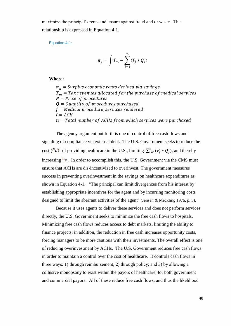
99
maximize the principal’s rents and ensure against fraud and or waste. The
relationship is expressed in Equation 4-1.
Equation 4-1:
∫ ∑
Where:
The agency argument put forth is one of control of free cash flows and
signaling of compliance via external debt. The U.S. Government seeks to reduce the
cost ( of providing healthcare in the U.S., limiting ∑ , and thereby
increasing . In order to accomplish this, the U.S. Government via the CMS must
ensure that ACHs are dis-incentivized to overinvest. The government measures
success in preventing overinvestment in the savings on healthcare expenditures as
shown in Equation 4-1. "The principal can limit divergences from his interest by
establishing appropriate incentives for the agent and by incurring monitoring costs
designed to limit the aberrant activities of the agent" (Jensen & Meckling 1976, p. 5).
Because it uses agents to deliver these services and does not perform services
directly, the U.S. Government seeks to minimize the free cash flows to hospitals.
Minimizing free cash flows reduces access to debt markets, limiting the ability to
finance projects; in addition, the reduction in free cash increases opportunity costs,
forcing managers to be more cautious with their investments. The overall effect is one
of reducing overinvestment by ACHs. The U.S. Government reduces free cash flows
in order to maintain a control over the cost of healthcare. It controls cash flows in
three ways: 1) through reimbursement; 2) through policy; and 3) by allowing a
collusive monopsony to exist within the payors of healthcare, for both government
and commercial payors. All of these reduce free cash flows, and thus the likelihood

100
of overinvestment. In this chapter, only reimbursement is considered as a mechanism
for controlling free cash flows. Policy and monopsony are discussed further in
Chapters 5 and 6.
The reduction in free cash flows via reimbursement is to ensure among other
things that positive NPV projects are chosen. The NPV projects in this scenario are
ones that are economically efficient and provide a positive return. The selection of
NPV projects by ACHs is distorted, as there is a moral hazard within the healthcare
market. The moral hazard in this case causes ACHs to compete on the quality or
perceived quality of goods, (Glied 2003; Nahata 2005).
4.1.3 Moral Hazard
Milgrom and Roberts (1992, p. 167) described a moral hazard as, “...the form
of post-contractual opportunism that arises because the actions that have efficiency
consequences are not freely observable and so the person taking them may choose to
pursue his or her private interests at others’ expense.” They felt that a moral hazard
could develop in any situation in which individuals are allowed or tempted to choose
an inefficient action, because the interest of the individual is not aligned with group
interests, and that action cannot be monitored easily. Milgrom and Roberts (1992)
suggested there are three conditions that must be present in an environment for a
moral hazard to exist:
1. There must be some potential divergence of interests between people.
2. There must be some basis for gainful exchange or other cooperation between
the individuals; in other words, there must be a reason for a transaction.
3. There must be difficulties in determining whether in fact the terms of the
agreement have been followed and in enforcing those contract terms. These
difficulties often arise because monitoring actions or verifying reported
information is costly or impossible.
Milgrom and Roberts (1992, p. 167) summarized the outcome in healthcare: “if you
are covered under health insurance or belong to a Health Maintenance Organization
(HMO), so that you are insured against all or most of the costs of visits to the doctor,
you are likely to make greater use of medical services of all kinds...”
The healthcare market in the U.S. is one in which those insured via private
insurance or government programs are at risk of overconsumption, or a “moral
101
hazard,” due to a lack of monetary risk in consumption. To be more succinct, when
payments are made by insurance companies or the government, the patient has no
incentive to minimize the consumption of medical services. Sometimes, even ACHs
have no incentive to minimize the supply of medical services.
Of course, this makes the demand for healthcare inelastic to price. People will
consume if they see a need/want to consume, even though the marginal cost of the
service could exceed the marginal benefit. The distortions within this market, via
public and private health insurance, shelter the consumers of medical services from
many of the financial consequences of their own decisions. The separation between
the prices paid by the patient and the actual cost of service leads to a moral hazard.
The existence of a moral hazard via health insurance is well documented in U.S.
healthcare by Milgrom and Roberts (1992), Pauly (1986), Gaynor (2000), Smet
(2002), and Glied (2003), among others.
Newhouse (1981) suggested that improperly structured insurance reduces the
amount of price competition in the marketplace, and thus the healthcare provider
competes on the basis of quality, as price is not a consideration in the consumption
equation utilized by the patient/consumer. This perspective is confirmed later by the
research of Wang (1999), Glied (2003), and Nahata (2005). “Studies have shown that
hospital payment arrangements lead to higher costs and contribute to lower
production efficiency by forcing hospitals to invest excessive amounts in technology,
provide more patient amenities, and provide excess services to attract physicians and
patients” (Wang 1999, p. 85).
The effect of the moral hazard of insurance leads to competition of the ACHs
for patients on other market parameters, such as quality. This leads to over-
acquisition of capital items, or the creation of programs that increase the perception of
quality. This need to compete on quality rather than price leads to an arms race, with
ACHs competing with newer/better equipment, technologies, and services. The
research of Robinson and Luft (1985) showed that this “arms race” generated 20
percent higher costs in the more competitive markets than in the less competitive
markets. This was confirmed by Smet (2002) and Glied (2003). Glied’s explanation
for higher costs follows:
“Studies through the 1980’s found that when many hospitals compete in the
same market, prices in that market is higher- not lower- than in setting with
102
fewer competitors. Competing hospitals engaged in a ‘medical care arms
race,’ buying more costly equipment than their neighbors. Consumers, who
both lack information about the value of this equipment for their condition and
who generally do not face full costs at the margin, select the hospital that
appears to offer the highest quality service.” (Glied 2003, p. 127)
While the healthcare market has tried to contain the moral hazard via
consumer cost sharing, ultimately the moral hazard distorts the market so that ACHs
are not required to compete for patients based upon costs. Instead, ACHs are forced to
use indirect means to gain consumer confidence, loyalty, and ultimately, more
patients. In other words, patients are not considering cost in their decisions to
purchase healthcare services; therefore, they have no incentive to choose the cheapest
or moderately priced care, but rather choose healthcare services based upon other
factors, such as quality or perceived quality (Newhouse 1981; Glied 2003; Nahata
2005). Because of this particular moral hazard, the scope for attracting customers is
changed and narrowed. Patients choose healthcare providers based upon service
offerings; in other words, based upon who offers the most comprehensive services.
This drives hospitals to enhance their images of quality via questionable projects, and
includes projects that have a negative NPV.
For the government, ACHs’ negative NPV projects can be projects that when
completed are considered underutilized due to low patient volume. This is considered
an issue of allocative efficiency. “Allocative efficiency problems arise in hospitals
when substantial resources are allocated to treatments of questionable effectiveness,
when unnecessary tests are employed, or when hospital clinical services are
underutilized due to low patient demand” (Wang 1999, p. 84). Wang et al. (1999)
recognized significant increases in excess hospital services from 1989 to 1993 that
could not be supported by efficient medical practices. They concluded that this
increase in spending within the market could have been caused by ACHs attempting
to gain market share. Their data showed excessive use of hospital capital resources in
the form of excess hospital services.
In the case of projects that are considered allocative inefficient, the cost for the
project must be recouped from the patients as a whole, which means that the
government ultimately is going to bear the cost for these types of investments pro-
rata. Considering that the U.S. Government consumed 65% of healthcare services

103
during the time frame of this study, one can understand their desire to restrict such
investments in order to decrease costs. When one considers that the government
ultimately will pay for a large proportion of such negative NPV projects (whether by
overinvestment or allocative inefficiency) via increased cost to the government, due to
the impossibility of creating a complete contract, the government is forced to utilize
indirect means of control. In this case indirect means, such as controlling the amount
of reimbursement, which typically are found where the agency relationship exists,
(Peterson et al 2006; .Conrad and Perry 2009).
4.1.4 Specialization
Specialization within healthcare further adds to the cost of agency within
healthcare. Hospitals provide specialized services within healthcare, which are
delivered by employees with focused training, such as doctors and nurses, who take
many years to obtain their qualifications. There is licensure for the practice, limiting
entry into the field for the physician and the nurse. In addition, the hospital itself has
acquired the right to provide healthcare services via licensing, and has acquired
specialized assets and technology to be able to deliver competent care to patients.
While there may be competition within geographic regions, it would be very difficult
to replace the entities providing the healthcare services.
Jensen and Meckling (1976, p. 33) recognized the importance of specialization
in the increase of agency costs in their study: "The size of the divergence (the agency
costs) will be directly related to the cost of replacing the manager. If his
responsibilities require very little knowledge specialized to the firm, if it is easy to
evaluate his performance, and if replacement search costs are modest, the divergence
from the ideal will be relatively small and vice versa." In other words, because ACHs
are such specialized units, it makes monitoring and replacement difficult. The
increased nature of specialization acts to increase agency cost with the healthcare
market.
4.1.5 Signalling
In contractual situations, agents signal their compliance or proper management
of the contractual arrangement. Often in cases with pre-contractual private
104
information, some of the privately informed people would gain if they could make
their information known. The difficulty is that there may be no simple, direct means
to reveal the private information. This creates incentives to find ways to convey the
information. One such strategy is via signaling.
Signaling may exist within the context of the U.S. healthcare market. The U.S
government lacks the resources to monitor individual hospitals adequately.
Therefore, it lowers its monitoring cost by using external monitors/lenders. Prior
research indicates that lenders/banks monitor borrowers. Banks monitor borrowers to
ensure that borrowers—in this case, the ACHs—are managing the business prudently
and efficiently so that the borrower may return the borrowed capital plus borrowing
costs. Often, banks require financial covenants that act as guidelines for the financial
performance of the firms. These financial guidelines, along with direct monitoring
via audits of the firm, ensure compliance with required firm financial performance.
Debt, according to Jensen (1986, p. 11), “increases efficiency by forcing
organizations with large cash flows but few high-return investment projects to
disgorge cash to investors. The debt helps prevent such firms from wasting resources
on low-return projects.” Furthermore, debt reduces the agency cost of free cash flows
by reducing the excess cash available to managers, thus reducing the likelihood of
overinvestment (Jensen, 1986). In the context of the agency problem between the U.S.
Government and ACHs, debt can be seen as a method of signaling efficiency to the
U.S. Government. Debt replaces direct monitoring costs for the government with
external monitoring via the lenders. The ACHs incur debt, among other reasons,
knowing that it signals to the government that they are being monitored on a regular
basis to ensure that they are running efficiently and are minimizing their investment in
negative NPV projects.
A corollary is that hospitals that provide more services to the government
would seek to send greater signaling of efficiency. Hospitals that derive larger
proportions of revenue from the government want to ensure that those streams of
revenues are not jeopardized, and are thus compelled to signal compliance with the
operational wishes of their largest customer. The government is trying to reduce
overinvestment or investment in allocative inefficient services. Typically, the
government encourages this through lower reimbursement to ACHs. Incentives to
align the goals of providers of healthcare services and insurers via payment schemes

105
or reimbursement schedules are well known (Peterson et al 2006; Eldridge and Palmer
2009; Melnick et al 1989; Conrad and Perry 2009; Lee and Zenios 2007). The ACHs
know that the government can and does change reimbursement for them. If there is a
risk of ACHs losing revenues because of the government’s need to reduce
overinvestment or allocative inefficient services, then the ACHs likely will want to
signal compliance with the government’s wishes, thereby ensuring that
reimbursement is not cut for their hospital or they are not subjected to planned
reimbursement schedules which may lower potential revenues. In effect, the ACHs
seek to show compliance so that they are not penalized by way of lower
reimbursements. Debt provides the mechanism for signaling compliance.
Therefore, one would expect a direct correlation of debt and hospital revenues
derived from providing government services. Hospitals with higher revenues from
government payors are at a greater financial risk should government change
reimbursement. For this reason, one would expect that as the proportion of
government-derived revenues increase, so too would the concern over ACHs’
vulnerability to changes in reimbursement. As the ACHs’ vulnerability increases, the
likelihood should be greater for the ACHs to want to signal efficiency.
We know that in most agency relationships, the principal and the agent will
both incur costs to ensure that the principal’s interests are protected. Principals will
incur monitoring costs, and agents often will incur bonding costs (Jensen & Meckling
1976; Chalkley and Khalil 2005; McLean 1989). In this case, bonding costs are the
costs incurred by the agent to guarantee to the principal that the agent will not take
decisions or actions that will harm the principal. In this case, the cost of debt can be
viewed as bonding costs, costs that the hospitals incur to bond themselves to the
principal (the U.S. Government). The debt that the ACH takes on acts as a guarantee
that the ACH (the agent) will not take actions in the form of overinvestment and
allocative inefficient services that harm the principal, in this case the government.
4.2 Agency Theory
4.2.1 Prior Research
In order to understand the agency relationship described earlier, a better
understanding of previous research is necessary. The purpose of this section is to

106
examine previous literature that has context and support for the agency argument put
forth within this chapter. The research presented here is meant to inform the reader of
previous academic works that have relevance to this study, and to draw parallels
between the previous literature and the argument presented within this chapter.
If one examines the ACH market and the agency framework that has been
discussed, one can see that what one has is a single principal, the government, which
hires many agents on its behalf, ACHs, to provide healthcare for citizens covered by
Medicare and Medicaid. From a broad perspective, this framework is similar to the
research conducted by Stephen Ross. In his research, Stephen Ross (1973) created a
set of utility functions under several relative payoff structures to examine the conflict
of Pareto efficiency (assuming perfect information) with the needs to motivate agents
within a principal-agent relationship. Ross concluded that payoff structures that solve
the principal’s problem and lead to Pareto efficiency, in which no further
improvement in efficiency can be made, are attainable and actually quite likely to
occur within the market. Effectively, Pareto efficiency can be attained by incurring
the cost necessary to ensure agent compliance. However, when there are many agents
acting on behalf of the principal, the fee may be the only communication between the
principal and the agent. In this case, Ross noted that while it may be feasible to
monitor the agents in action, it would be too expensive. This is very similar to
conditions within the ACH market, where in this case, the government’s only
mechanism for communication is the reimbursement rate. The government would
like to be able to ensure compliance via monitoring costs; however, similar to one of
the conclusions reached by Ross, the economic viability of such a system for
monitoring is not there, as the cost are too great. Ross (1973) also supports the
general principal that agency costs may be present in any agency relationship and that
agency relationships may be found in any contractual arrangement where a principal
contracts with an agent to act on the principal’s behalf.
Jensen and Meckling (1976) brought agency theory to the forefront of finance,
as their work combined agency theory, property rights theory, and the theory of
finance to provide a theory of ownership of the firm. They defined the concept of
agency costs in light of the separation of ownership and control, that is, between the
principal and agent, together with the associated costs of the relationship. They
created a model of the firm with equity and debt and examined the resulting agency

107
costs. They suggested that the principal could act to monitor the agent to limit the
deviation of the agent’s dealings from those that are in the best interest of the
principal. Additionally, they suggested that it is beneficial for the agent to incur
bonding costs in order to guarantee to the principal that the agent will not take actions
out of line with principal’s interest. In their model, both monitoring and bonding costs
were considered agency costs, along with the residual loss.
This research uses the Jensen and Meckling (1976) model of agency costs, and
argues that ACHs take on bonding costs, in effect signaling behavior, which limits
deviation from the principal’s interests. Bonding reduces monitoring costs, and where
debt is being used, the reduction in free cash flows limits the options of the agent
(ACHs) and therefore minimizes the likely cost of aberrant activity.
Jensen (1986) expanded agency theory, incorporating discussions of the
agency costs of free cash flows and corporate finance. Free cash flows were defined
by Jensen (1986, p. 323) to be, “cash flows in excess of that required to fund all
projects that have positive NPVs when discounted at the relevant cost of capital.” He
analyzed the conflict between managers and shareholders and the role of reducing free
cash flows under managerial discretion in diminishing the conflict between the
principal and the agent (management). Jensen (1986) suggested that debt is a signal
and a way of reducing the manager’s discretion of the use of free cash flows. Jensen
covered two important points related to this research on agency costs: 1) the benefits
of debt in reducing agency cost of free cash flows; and 2) how debt can substitute for
dividends.
These two points of agency are important to this research and should be
discussed further. The first is that managers with excess free cash flows can signal to
shareholders by declaring a permanent increase in the dividend. However, according
to Jensen (1986), this is a weak promise, as dividends could be changed in the future.
Secondly, debt can enable managers to bond their promise to the payout of future cash
flows; thus, debt can be an effective substitute for dividends. Jensen suggested that
debt reduces the agency costs of free cash flows by reducing the resources under
management’s control, and is thus likely to reduce overinvestment.
Jensen’s (1986) theory suggested that firms with large amounts of free cash
flows that are allowed to accumulate under the firm management’s control are more
likely to be wasted on projects/mergers that are of minimal value to the firm and

108
possibly even value destroying. This is an important result, because this research
suggests that a similar agency problem exists between the CMS and ACHs in the U.S.
The ACHs are similar to the firm with prior large free cash flows. Due to the ACHs’
need to compete on quality as well as the characteristics Jensen describes, ACHs are
likely to overinvest or invest in allocative inefficient services, as discussed previously.
In the case where ACHs overinvest, they are likely to increase the cost to their
customers to cover the overinvestment. Government costs will increase, because the
CMS consumes the majority of healthcare. However, if the government (principal) is
able to reduce the resources under management of the ACH (agent), then the ACH is
more apt to operate efficiently and ensure that projects are scrutinized for value
creation and allocative efficiency. This effort effectively aligns the goals of the
principal and agent.
Kim and Sorensen (1986) analyzed the capital structures of firms in relation to
insider ownership of public firms. They extended Jensen and Meckling’s (1976)
work by looking at firms with multiple shareholders, and testing empirically for the
presence of agency costs and how these costs relate to capital structure. They used a
sample of 186 companies divided into groups with high inside ownership (above
25%) and low inside ownership (below 5%). The groups then were broken into
separate industries so that only like industries were compared. Using analysis of
variance (ANOVA) and simple regression, they found that firms with insider
ownership had 6% to 7% higher debt to total assets than those of lower inside
ownership within the same industry. These findings are relevant to this research, as
they indicate that debt levels and agency effects are related in the way that Kim and
Sorensen's (1986) theory predicted that firms with high inside ownership have lower
agency costs. This is supported by the views of Jensen and Meckling (1976), who
suggested that owner/managers have little or no agency costs.
Wedig et al. (1988) also used this agency framework to analyze the capital
structure of hospitals in relation to ownership structure. Hospitals in the U.S. are
categorized as either non-profit or profit based hospitals, and the majority are non-
profit. Wedig et al. suggested that capital structure is an interesting subject in light of
the fact that nonprofit hospitals are exempt from tax, yet maintain debt obligations,
even though there are no tax advantages from doing so. According to Wedig et al.,
the bulk of revenues within hospitals are derived from public or private insurers, and
109
this reimbursement mechanism affects the cost of both debt and equity. They
examined how capital structure is affected by the reimbursement policies of the major
insurers, taking into account differences in ownership structure. In addition, they
assessed the debt/asset ratios of hospitals and determined the roles that reimbursement
policies, tax policy, and bankruptcy risk play in capital structure. Wedig et al.
concluded that hospitals with high reimbursement via cost-based reimbursement have
greater debt than hospitals with a lower reimbursement mechanism. They suggested
that this would be a problem going forward if reimbursement is reduced. They also
concluded that the type of ownership provides for no differences in capital structure,
even in light of the differences for holding such debt. This is important to the
research as no variable within the data allows for ownership structure.
McLean (1989) examines the application of agency theory to healthcare
organizations. He suggests that although agency theory was developed as a
theoretical model for use in economics and finance, it is applicable for use by
managers of healthcare organizations and policy makers. McLean states “several
types of arrangements used to finance healthcare organizations can be understood as
ways of dealing with agency problems” (McLean 1989, p.65). He suggests that
unequal access to capital amongst providers may be a result of varying degrees of
agency costs. McLean (1989) applies his theory of agency in healthcare to hospital
based medical care in the U.S. examines the participants within the healthcare market
and describing how agency theory fits. He suggests that hospital managers show
signs of agency problems when they use their managerial discretion to consume
perquisites to a greater extent than allowed by contract, a perfectly plausible event in
healthcare, which creates opportunity for abhorrent behaviors due to the lack of
monitoring output or the amount of input into health services. Debt according to
McLean (1989) helps resolve problems of agency in healthcare in a way described by
Jensen and Meckling (1976) by reducing the resources under managements’ control
as cash flows must be promised in order to acquire debt. McLean suggests that
providers of healthcare are temporary agents that have a propensity to over consume
perquisites in the form of reduced effort and or higher fees. This is made possible by
the monitoring problem within healthcare. McLean (1989) concludes that agency
theory is applicable in many cases to healthcare.
110
McLean’s discussion is important to this research as it supports the theoretical
application of agency theory to the U.S. healthcare market, specifically addressing the
relationship between patient and provider, payor and provider and physician/ provider
relationships. He further suggests that agency cost may explain the unequal access to
capital by providers.
While no direct agency costs are attributed to the unequal access to capital, the
inference that it can have impact on access to capital is important. This research puts
forth the premise that agency cost of free cash flows impacts decisions of capital
structure by limiting payments to ACHs and thereby limiting the amount of cash
flows with which they can promise in order to obtain debt. The outcome of this
limitation in the available cash flows to support borrowings, limits the debt capacity
for an ACH. The inequality is driven by ACHs, which have differing cash flows to
promise, which means that ACHs with better cash flows can obtain more debt, while
those with lower cash flows have less. This will be discussed further later on.
Eisenhardt (1989) assessed agency theory and reviewed the empirical
literature to determine the strains of agency research that provide testable positions
and to evaluate empirical agency theory. She concluded that there are two strains: (1)
positivist, examples of which are Berle and Means (1931), Jensen and Meckling
(1976), Fama (1980), and Fama and Jensen (1983), which is interested in describing
governing mechanisms that minimize or remove agency costs; and (2) principal-agent
research, examples of which are Anderson (1985), Eisenhardt (1985, 1988), Eccles
(1985), and Conlon and Parks (1988), which is concerned with empirical research of
the principal-agent relationship. According to Eisenhardt (1989), principal-agent
research provides greater opportunities for empirical testing.
She separated the two strains of research by noting, “Positivist theory
identifies various contract alternatives, and principal agent theory indicates which
contract is the most efficient under varying levels of outcome uncertainty, risk
aversion and information…” (Eisenhardt 1989, p. 60). She concluded with five
recommendations for research within the principal-agency model: 1) focus on
information systems, risk, and outcome uncertainty; 2) focus on theory relevant
situations in which contracting problems are difficult and agent opportunism is high;
3) expand into richer contexts and apply agency to organizational situations where
asymmetric information is present; 4) use agency as a complement to other theories;
111
and 5) look beyond economic literature. The research in this chapter follows many of
the guidelines laid out by Eisenhardt (1989) and recognizes the strength in applying
agency to real market/contractual situations within the healthcare market.
Stulz (1990) analyzed financing policies, observing how they restrict
management’s self-interested behaviors in the presence of asymmetric information.
He constructed a model of an atomistic shareholder who did not have access to the
firm’s cash flows, nor insight into management’s investment decisions. Stulz assumed
that it was too expensive for shareholders to demand dissemination of cash ex-post.
He then suggested that managers enjoy increasing perquisites with an increase in
investment, even when it involves negative NPV projects, so consequently, managers
always will choose to invest rather than pay out cash. Informational asymmetries
under these conditions cause problems for firms with too little cash flow to invest in
positive NPV projects, as managers lack credibility in convincing the shareholders
that they do not have enough cash flow to take advantage of the positive NPV
opportunities.
Stulz (1990) concluded that financing policy reduces the agency cost of
managerial discretion. Agency cost of managerial discretion has two costs:
overinvestment and underinvestment. Stulz found that debt that requires management
to pay out funds from cash flows, which exacerbates the underinvestment costs. An
increase in underinvestment cost is a reduction in overinvestment costs. Stulz
confirmed the premise put forward in this research: Government can drive down
overinvestment by ACHs by reducing free cash flows to ACHs.
Calem and Rizzo (1995) analyzed the agency cost of capital markets in U.S.
hospitals. They suggested that investment activity is related closely to the liquidity or
internal funds of the hospital, which can determine access to debt markets. They
pointed to previous research of Sandrick (1986) and Wilkinson(1988) to suggest that
access to debt markets at the time of the study was becoming difficult, driven by
various cost containment methodologies by insurers which lowered hospital operating
112
margins and thus liquidity (Calem and Rizzo, 1995).5 They suggested that there may
be a causal relationship between investment activity and the availability of internal
funds. Using a balanced panel data set of 1,400 hospitals from 1985-1989 and GLS
regression analysis, they postulated that small hospitals and freestanding hospitals
were more likely to encounter financing constraints in comparison with large
hospitals or multi-hospital chains. By separating the hospitals by size and chain
affiliation, they examined the relationship of liquidity and investment. Measuring
investment by way of the change in fixed assets from one period to the next, and
controlling for labor, labor to capital, occupancy of beds, market growth, credit
standing, and marginal revenue of product, they used a fixed effects model to regress
investment against liquidity and control variables. Results from their regression
analysis concluded that small hospitals and freestanding hospitals face borrowing
constraints due to agency costs as liquidity was closely related with investment in
small and freestanding hospitals. This is in contrast to their finding that large
hospitals do not, as the internal liquidity of large, multi-chain hospitals did not
correlate to investment. While Calem and Rizzo (1995) were not analyzing Agency
Costs of Free Cash Flows as suggested in this research, but rather Agency Costs of
Capital Markets, it is important to notice that they reference underlying payment
methodologies as primary reasons for increased difficulty in access to debt markets
and as a consequence making select ACHs more reliant on internal fund for
investment. It is interesting to note that the premise suggested under the existence of
agency cost of free cash flow may actually increase agency costs of capital markets as
described by Calem and Rizzo (1995). It is the effect of these payment
methodologies on free cash flows and the consequence of such changes may lead to
difficulties in ACHs obtaining debt to fund new investment, therefore leaving them
more reliant on internal funds. Additionally, this research may provide evidence of a
5 Calem and Rizzo primarily point to the Prospective Payment System, implemented by Medicare
in 1984 as the primary example of cost containment via payment methodologies. The Prospective
Payment System provided a fixed level of payment for specific services regardless of the hospitals
actual charges. This payment arrangement increased the hospitals risk of incurring uncovered charges
and therefore lowered margins on those services.

113
different type of agency cost that affects hospitals, which is acting as a primary driver
for increasing the agency costs of capital markets.
Leland (1998) considered the optimum amount and maturity of debt for a firm.
He noted that the agency costs of debt related to the asset substitution problem
(Jensen & Meckling 1976) are significantly less than the tax advantages provided by
debt. Therefore, firms will position themselves by taking on the optimum level of
debt regardless of the value transferred to the bond holders because of the risk
reduction value presented in debt.
Parrino and Weisbach (1999) suggested that the optimum leverage for a firm
is when the incremental increase in the cost of debt via agency costs equals that of tax
benefits for the increase in debt. They suggested that overinvestment is more likely in
firms with stable cash flows and little growth opportunities. They concluded that the
stockholder/bondholder conflict affects debt levels, and that this distortion usually
increases as the debt levels increase. Their findings also concluded that the agency
cost of debt can be large and can vary greatly across firms. This is important, as
ACHs have stable cash flows and few growth opportunities. Therefore, if ACHs have
few growth opportunities, they are more likely to have overinvestment.
Rivenson (2000) considered the liquidity of hospitals and the differences
between non-profit and for-profit hospitals, as well as what strategies are used by
ACHs to determine their cash position. Through public data and interviews, they
concluded that the cash reserves were increased deliberately by nonprofit ACHs,
mostly derived from previously built-up reserves that subsequently had been invested,
as well as improved payables and receivables policies. They suggested that in light of
the anticipated future reduction in reimbursement by the public and private insurers,
ACHs have been holding greater cash reserves. Accordingly, this increase in cash
reserves and investments serves to supplement earnings from healthcare services, and
to provide access to capital markets and a lower cost of capital (Rivenson 2000).
Harvey et al. (2003) analyzed the effect of capital structure on limiting agency
costs. They suggested that debt creates value for firms that have high agency costs,
especially when the debt reduces the likelihood of overinvesting. Using 1,014
exchange listed firms from emerging markets, and including ownership and stock
return data, Harvey et al., using a three-stage least squares regression model,
concluded that debt mitigates the reduction in firm value that is induced by

114
asymmetric information between the principal and agent, in this case management and
stockholders. This is accomplished by reducing the overinvestment problem by
increasing debt.
Morellec (2004) analyzed the impact of managerial discretion and corporate
control mechanism on debt levels and the value of the firm. Capital structure in the
study incorporates the tax advantage of debt minus bankruptcy and the agency costs
associated with management discretion. Morellec uses a contingent claims model to
analyze the relationship between debt and management discretion (assuming
managers obtain perquisites from investment). He analyzed the impact of
management’s opportunistic behavior on leverage policy, asset values, and firm value.
He concluded that principal-agent conflicts via the manager-shareholder relationship
explain the lower debt levels experienced in real firms, as well as the fact that firms
with high growth opportunities carry less debt. He also suggested that these agency
conflicts could explain the apparent cross-sectional variation in capital structures.
Morellec supported the position that principals can and do benefit from a reduction in
free cash flow.
Harvey, Lins, and Roper (2004) conducted tests on data from emerging market
firms’ ownership structures to see which would lead to large/extreme agency costs.
They used both traditional financial statement data and global debt contract data to
analyze the premise that debt should create value in firms with high expected agency
costs. To measure a firm’s potential overinvestment tendency, they used higher levels
of assets in place and limited growth opportunities. Cross-sectional tests utilizing
financial accounting data revealed that leverage mitigates losses in a firm’s value.
They reported that the benefit of leverage is concentrated in companies that have
limited growth opportunities or have a higher percentage of assets in place. This
suggests that there is evidence of large-scale recognition that debt can minimize
overinvestment, thus creating value for the principal. The work of Harvey, Lins, and
Roper is applicable directly to this research, as the argument put forth in this study
recognizes that ACHs’ management may signal efficiency to government payors, and
in doing so minimize overinvestment by the ACHs, thereby creating value for the
government via savings, as described earlier.
Iacobucci and Winter (2005) analyzed the incentives for asset securitization
that are driven by informational asymmetries within a corporation. They defined
115
asset securitization as the partial or complete segregation of a specific set of cash
flows from a corporation’s other assets, and the issuance of securities based on these
cash flows. Under their findings, asset securitization enhances monitoring efficiency
by reducing noise in the relationship between firm and managerial performance, and
consequently the agency cost of free cash flow, which is supported by Jensen (1986).
In the context of this research, the increase in monitoring efficiency comes at
the expense of small ACHs. According to Calem and Rizzo (1995), small and
freestanding hospitals face borrowing constraints due to agency costs. He noted,
“From a policy perspective, the results suggest that efforts to limit payments to
hospitals during the past decade may have been particularly onerous to the investment
decisions of small hospitals and free standing ones. Such hospitals, we find are more
dependent on their own liquidity for investment funds” (Calem and Rizzo1995, p.
1012). Borrowing constraints upon small hospitals are created by efforts to limit
payments to hospitals, as discussed by Calem and Rizzo (1995), and this is evident in
the data provided in this research, as small hospitals consistently show lower debt
than other larger sized facilities. When looking at debt measurements from Chapter 3,
Category 1 hospitals (those with less than 100 beds) had less debt. Category 1 sized
facilities showed the lowest debt to equity ratio, with a value of 0.73, and the second
lowest debt ratio, with a debt ratio of 0.45. Calem and Rizzo suggested that limitation
in payments is the underlying cause of these constraints. The findings in Chapter 3
also suggest that larger hospitals are better able to reduce the effects of agency.
Chalkley and Khalil (2005) utilizing an agency theory framework between
insurers and providers (ACHs) demonstrate that monitoring schemes differ in their
effectiveness in utilizing patients as a disciplining mechanism and showed that the
choice of the type of monitoring tool itself may depend on the strength of the patients
change in demand to variation in quality of service. The agency framework used in
their research assessed two fundamental ways of calculating payments, one based
upon input measures (treatments) the other on output measures (health outcomes or
improvement to health statusThey showed that when demand is responsive to quality
of service, payment mechanisms based upon outputs or outcomes, reduce the overall
cost to the insurer when compared against payment mechanisms based upon treatment
or inputs. They suggest that this is because payments based upon outputs or outcomes
make misrepresentation of the type of patient being treated more costly to the

116
provider in terms of demands for services, because services rendered will have to be
tailored to the patient type such that the outcome is consistent with what was
originally claimed by the provider.
The research of Chalkley and Khalil is important to this research in several
ways, one is that they recognize the Agency relationship between insurers and ACHs.
The government is the largest insurer and consumer of health services in the U.S.
They in effect hire agents (ACHs) to act on their behalf to treat patients. The
principal-agent relationship is one in which monitoring is difficult. This difficulty in
monitoring means that the principal must incur monitoring costs in order to limit
abhorrent behavior by the agent, in this case providers. The second key point from
the research of Chalkely and Khalil (2005) extends this last point. They recognize
that payors may be able to reduce agency costs through payment schemes to providers
(ACHs). This research suggests two forms of symptoms of the agency relationship
may be present within U.S. healthcare, signaling and agency costs of free cash flows.
In this case, signaling by ACHs maybe an effort on their part not to be subjected to
payment schemes as described in Chalkley and Khalil (2005) and likewise agency
costs of free cash flows may likely be a form of agency costs incurred by those ACHs
already being subject to payment schemes.
Nahata et al. (2005) examined the moral hazard within U.S. healthcare. They
analyzed the demand for medical services in relation to out-of-pocket expenses by the
insured. Their assumption was that a third-party insurer always is involved in the
consumption of the healthcare services. They incorporated the demand inelasticity of
medical services, in which any increase in medical services could be passed on
directly to the consumer. Using a broad range of elasticity, a utility function (utility
maximization model) was created to analyze demand under various conditions. The
finding was that cost sharing between the consumer and insurer is the single most
important factor in limiting the rise in medical expenditures. Their findings support
the notion that providers do not compete based upon price, but rather on quality or the
perception of quality.
As described by Nahata et al. (2005), the moral hazard in the healthcare
markets is one of the prime reasons that ACHs compete on quality or perceived
quality, and thus have a propensity to overinvest, as discussed previously. Like “loss
leaders” in retail, the investments by ACHs are not always to generate a direct return

117
on the investment, but rather work as an indirect means of increasing patient volume,
and thus revenues. Under this scenario, the CMS ultimately will carry the burden of
those losses in its request for additional reimbursement, or perhaps greater quantity of
services rendered. Ideally, by reducing the amount of free cash flows available to
hospitals, the CMS curbs ACHs’ ability to overinvest.
Peterson et al (2006) provides a review of 17 empirical studies, from 1980 to
2005, on pay for performance in healthcare to examine the effect of explicit financial
incentives on measures of the quality of health care services. Pay for performance
was a concern as they point to the poor quality of healthcare in the United States,
suggesting via a report from the Institutes of Medicine (2001) that numerous factors
contributed to the poor quality of health services including the structure of the present
healthcare payment system. CMS along with private payors have been using explicit
financial incentives to try to induce quality, but questions remain as to the
effectiveness, optimal design and implementation needed to be answered. Peterson et
al (2006) suggest that the provider patient relationship is a type of principal agent
relationship. The principal (the patient) cannot directly observe or know the level of
skill or effort expended by the agent (the provider) doing the contracted work.
Because of this lack of information on the part of the principal (the patient), they do
not have knowledge of their own medical condition, how much care they need and or
expected outcomes of services rendered, so hence rely strictly on their agent to
perform these action/services. Because of the asymmetry of information on need and
outcome for healthcare services, demand for healthcare services maybe unresponsive
to quality. In this light, performance-based pay or explicit financial incentives may
provide an answer when patient demand is unresponsive to quality. Peterson et al
(2006), conclude that providers are paid the same regardless of quality of the
healthcare they provide, producing no financial incentives for quality and in some
cases disincentives. Based upon the literature search conducted they suggest that
performance based pay provides a real opportunity to align both principal and agent
interests using incentives for the agent.
Schneider and Mathios (2006) expanded the application of principal agency
theory to health services. They used a principal-agent framework to examine the role
that monitoring costs faced by an insurer had on healthcare utilization. Using a
theoretical model to consider an alternative to incentive-compatible contracting, they
118
proposed for the insurer to actually monitor the care prescribed by providers under a
fee for service arrangement. They compared ACH length of stay for fee for service
patients with those of capitated patients in both high and low monitoring conditions.
Looking at the variance in length of stay, they assumed high monitoring costs with a
higher variance in length of stay for a given procedure. Their theoretical model
develops predictions for healthcare utilization for fee for service arrangements in
cases of both low and high monitoring costs. Testing predictions of the theoretical
model via utilization using length of stay measures in their the research; they compare
outcomes of those treated by providers under a fee for service arrangement with those
treated under a capitated plan. Utilizing the two basic types of insurance plans within
the U.S, traditional indemnity (fee for service) and managed care (capitated), they
suggest that capitated plans transfer the financial risk of treatment from the insurer to
the ACH. This provides an excellent example to implement and how the incentive
compatible contract to contain excessive use of services (measure by the length of
stay) can be used to contain agency costs. Using principal-agent theory, they suggest
that this transfer of risk from the insurer to the provider maybe expensive if the
provider is risk averse. This may be a problem as incentive compatible contracts may
cause the provider to not be as good an agent for the patient or the insurer, which
might lead to a condition of the under provision or lack of quality of care depending
on how risk averse the provider is.
Bazzoli et al. (2006) examined ACHs’ financial performance from 1993-2000,
separating the study into two time frames. They analyzed financial data accumulated
from the CMS cost reports and the survey data from the AHA. Using this
information, their sample was divided into groups: those considered financially
strong, and those considered financially weak. Performance was dictated by the use
of profit margin and ACH cash flows with strong or weak performances, divided at
the twenty-fifth and the seventy-fifth percentiles. Over time, performance was
examined to understand better whether strong hospitals were getting stronger and
weak hospitals were getting weaker.
Bazzoli et al. (2006) concluded that the strong hospitals were not getting
stronger over time, as the very highest performers at best were maintaining their
financial performances, while the weaker institutions were performing worse at the
end of the longitudinal study. Weaker hospitals were found mostly to be rural

119
hospitals (Morellec & Smith 2007). This is consistent with Calem and Rizzo (1995),
who found that small rural hospitals face borrowing constraints due to agency costs.
The evidence for Calem and Rizzo is shown in thefindings of Morellec and Smith
(2007), which provided evidence that the restriction or constraints on borrowing is
most likely the result of the lack of profit margin and consequently free cash flows
within this dimension of the U.S. ACH market.
Eldridge and Palmer (2008), conduct a systematic review of current literature
on the topic of performance-based payments as a methodology to improve the
performance of health systems in low-income countries. The use of performance-
based payments had recently become a popular methodology to achieve specific
health targets in low-income countries. In their research, they find performance based
payments as the primary approach used to resolved problems of the principal agent
relationship. They describe the principal-agent relationship as “one in which an actor
(the principal) can act more effectively by relying on the services of a so-called
“agent” whose utility function differs in some sense from the principal, meaning that
they cannot be relied upon to act in entirely the way desired by the principal”
(Eldridge and Palmer 2008). The problem, as they suggest for the principal, is how
best to create a contract that will incentivize or motivate the agent to behave in the
desired manner required by the principal, even when the principal cannot monitor
outcomes or output. Recognizing that many health systems in the developed world
are adopting this approach and have made great strides in moving from input based
budgets to fee-for-service models, including payments based upon diagnosis-related
groupers. Using the research of Peterson et al (2006) they suggest that performance-
based pay has been found to have generally positive effects in aligning incentives ,
but recognize that adverse activities such as gaming are still of concern. They
conclude by recognizing some of the success of performance based payments but
provide for some concern in utilizing these methodologies in low-income countries as
these methodologies transfer risk to the providers of healthcare services, which are
working in more challenging or fragile settings. Where monitoring is difficult,.they
suggest it may be difficult to define proper performance and how to measure it,
whether the targets are achievable and more importantly how incentives via payments
may skew activities and the performance of the providers in a way that may be
detrimental to the local health services long-term.
120
Conrad and Perry (2009) asks the question, utilizing a conceptual theoretical
framework drawn from microeconomics, behavioral economics and agency theory,
whether financial incentives can improve the quality of healthcare services. They
analyze eight propositions in their research. (1) Rewards vs Penalties, (2) Nature of
Incented Entity and Focal Quality Behavior, (3) General versus Selective Incentives,
(4) Extrinsic versus Intrinsic Motivation, (5) Relative versus Absolute Performance
Incentives, (6)Size of Incentives, (7) Certainty of Incentives and (8) Frequency and
Duration of the Incentive Payoffs. They conclude that properly designed incentives
can improve the quality of healthcare services along the dimensions of structure,
process and outcomes. However, they suggest that under the current market structure
for healthcare services, incentive-induced improvements to quality of healthcare
services are likely to be small.
The Conrad and Perry (2009) paper is important to this research as their
approach recognizes and considers the principal-agent relationship and the need to
align incentives between the principal, the payor in their research with the agent, the
provider via payment methodologies. The alignment of incentives and solving agency
problems within the healthcare market between CMS (a government payor) and
ACHs (a healthcare provider) is one of the primary considerations of this research.
The recognition of this problem by other researchers suggests an understanding of the
principal-agent problem between CMS and ACHs and a need to align incentives via
payments as a valid strategy, supports the premise of this chapter that agency costs
may exists and the government may be trying to solve these via reimbursement
strategies. Likewise, that agents may be trying to reduce agency problems and costs
by bonding (signaling).
4.3 Data
4.3.1 Description of the Data
Data used in this study was collected from the CMS, and is referred to most
often as the MCR. The MCR contains provider information such as facility
characteristics, utilization data, cost and charges by cost center (in total and for
Medicare), Medicare settlement data, and financial statement data. The CMS
maintains the cost report data in the HCRIS. A full description of the data was
121
provided in Section 3.4 of Chapter 3, and a list of ratio variables was provided in
Section 3.5.2.
Additional variables were created for analysis in Chapter 4. A description of
the variable, its creation, and its use is discussed below. A table of all variables used
in Chapter 4 can be found in Table 4.1. Separate variables were used for signaling
and agency cost of free cash flows.
No breakdown by certain characteristics, i.e. for-profit/ non-for-profit, is
possible, as the variables necessary to do so are not contained in the data.
4.3.2 Additional Variables
This chapter proposes two separate models of agency: one for signaling, and
the other for agency cost of free cash flows. In both models, the percentage of
government business, (%Gov_Bus) is used as a primary variable, in the case of
signaling the dependent variable and for agency cost as the primary independent
variable. Therefore, it is important to understand how this variable is calculated.
Due to the formatting and information of the MCR, we were not able to get
direct information of what percentage of the ACHs’ revenue is derived in dollars from
government sources, and so a proxy had to be established. The variable %Gov_Bus is
a proxy, using inpatient and outpatient days from government payers as a percentage
of total inpatient and outpatient days/visits for all payers accepted by the ACH as
reported by the MCR for each year. Government payors include Medicare and
Medicaid, amongst others. While this does not provide exact dollar reimbursement or
revenues from government sources, it did allow this study a proxy of those revenues.
As government payers pay inpatient services by a DRG, each DRG has a length of
stay measure associated with it. The length of stay measure quantifies the maximum
allowable number of days recognized by the government for a given DRG. Each
DRG is paid a flat fee that takes into account the appropriate number of patient days
utilized by the DRG. Outpatient procedures are delivered via a patient day.
Normally, one has no overnight hospital services, and is counted as outpatient.
Because the payment can be equated to patient days, this allowed us to take the
percentage of patient days consumed by the government of total patient days and
directly correlate it back pro-rata to free cash flows. While this was not an exact
match, it provided a good proxy. This is not to say there are not limitations to the
122
proxy to accurately represent the percentage of revenues derived from government
payors. Government payors reimburse less than private payors for services rendered
by ACHs, so ACHs may be receiving higher reimbursement for those patient days
sold effectively to private payors for each patient day. This will have some tendency
to mean the actual revenues derived from the government may be overstated slightly.
However this is expected to be minimal as the government reimburses on average
around 25 % to 27% of charges where private payors reimburse on average around
30% of charges according the claims data used later in this research.
The MCR provided the necessary variables to calculate %Gov_Bus, which is
defined as the sum of Title XVIII and Title XIX, divided by total inpatient/outpatient
days. Title XVIII is defined as Medicare (Social Security Agency). Title XIX is
defined as Medicaid (Social Security Agency). The CHIPS program was ignored for
the purposes of this research, as it was deemed small, and most importantly, not all
ACHs participate in it. Government employees also were excluded, as the amount was
relatively small and not definable from a research perspective.
Total Inpatient/Outpatient Days is defined as the total number of patient days
produced by the ACH for that year on both an inpatient and outpatient basis. Total
Inpatients/Outpatients had a total N of 53,240 out of 55,582, with 2,342, or 4.2%
missing. As Total In/Outpatient Days is a given number from the MCR, these cases
were dropped. Using Tukey’s (1977) definition, outliers and extremes are those with
values above 100,707 Day/Visits, and a total of 34% of the cases were categorized as
extremes.
The extremes were allowed to remain in the study, as the highest Day/Visits
was 582,274 patient days/visits, which is possible with a hospital with 1,595 beds.
Also in consideration for this decision was the fact that Total In/Outpatient
Days/visits also is comprised of outpatient visits, which do not required a hospital
bed to provide healthcare services.
The Total In/Out Days/Visits on the other prospective end with a value of zero
were excluded, as the hospital was considered non-operational for this portion of the
study. For %Gov_Bus = (TitleXVII + TitleXIX) patient days/(Total In/Outpatient
Days), N= 50,095 with 5,487 missing. The %Gov_Bus is a calculated variable, so
missing data is due to missing data in the underlying variables in the MCR used to
calculate %Gov_Bus.

123
The mode of %Gov_Bus was close to 1.00. Initially, this value was of
concern; however, upon further review, it was determined that the majority of ACHs
with values close to 1.00 were highly correlated, with a value of 1 in (num_bed_cat),
which described ACHs in the category with the lowest number of beds, between (0-
100) beds. These hospitals tend to be in rural areas, where few have private
insurance, and reimbursement is derived primarily from Medicare and Medicaid.
All negative values for %Gov_Bus were rejected, as negative values for this
variable were considered invalid. All values for %Gov_Bus had to be greater than
zero (%Gov_Bus > 0). All missing values were ignored, and those cases were
omitted from the study. Methodologies for the analysis of both signaling and agency
costs of free cash flows were similar; however, they will be addressed separately.
4.3.2.1 Variables included in Signalling Models
Figure 4.1: Signaling Variables:
Shows the variable to be included in the signaling model. This figure provides the variable name and the definition of calculation of the variable. In addition, it provides the actual variable name used in the data. All variables were calculated with the exception of fiscal year. Multiple variables are used for some variable categories. For example, Leverage has four underlying actual variables that are used in the modeling. This was done so that the modeling could observe the relationship of %Gov_Bus and multiple definitions of leverage. A full list of variables for Chapter 4 is available in the Appendix to Chapter 4. The list provides variable name, nomenclature, whether the variable was calculated or provided with the data itself and a definition of the variable.
Signalling Variables
Variable Name Actual Variable Definition
% Gov Bus % Gov Bus CMS patient days /Total In/Out patient days
Leverage
Leverage Total Longterm Liabilities/Total Assets
Leverage_2 Leverage ( non-negative value)
Debt/Equity Total Debt /Equity
Debt Ratio Total Liabilities/ Total Assets
Profitability
Net Margin Net Income/ Sales
Cash flows
Operation Cash Flows FCF + CAPEX
Liquidity
Liquidity Current Assets/ Total Assets
Size
LnTA Natural Log of Total Assets
Time
Fiscal Year Fiscal Year Reported
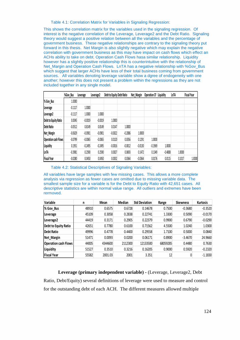
124
Table 4.1: Correlation Matrix for Variables in Signaling Regression:
This shows the correlation matrix for the variables used in the signaling regression. Of interest is the negative correlation of the Leverage, Leverage2 and the Debt Ratio. Signaling theory would suggest a positive relation between all the variables and the percentage of government business. These negative relationships are contrary to the signaling theory put forward in this thesis. Net Margin is also slightly negative which may explain the negative correlation with government business as this may have impact on cash flows which effect an ACHs ability to take on debt. Operation Cash Flows hasa similar relationship. Liquidity however has a slightly positive relationship this is counterintuitive with the relationship of Net_Margin and Operation Cash Flows. LnTA has a negative relationship with %Gov_Bus which suggest that larger ACHs have less of their total business coming from government sources. All variables denoting leverage variable show a dgree of endogeneity with one another; however this does not present a problem within the regressions as they are not included together in any single model.
Table 4.2: Statistical Descriptives of Signaling Variables:
All variables have large samples with few missing cases. This allows a more complete analysis via regression as fewer cases are omitted due to missing variable data. The smallest sample size for a variable is for the Debt to Equity Ratio with 42,651 cases. All descriptive statistics are within normal value range. All outliers and extremes have been rermoved.
Leverage (primary independent variable) - (Leverage, Leverage2, Debt
Ratio, Debt/Equity) several definitions of leverage were used to measure and control
for the outstanding debt of each ACH. The different measures allowed multiple
%Gov_Bus Leverage Leverage2 Debt to Equity Debt Ratio Net_Margin Operation CF Liquidity LnTA Fiscal Year
% Gov_Bus 1.0000
Leverage -0.1117 1.0000
Leverage2 -0.1117 1.0000 1.0000
Debt to Equity Ratio 0.0045 -0.0019 -0.0019 1.0000
Debt Ratio -0.0512 0.8149 0.8149 0.0147 1.0000
Net_Margin -0.0629 -0.0901 -0.0901 -0.0022 -0.2086 1.0000
Operation cash Flows -0.0799 -0.0065 -0.0065 0.0120 0.0356 0.1291 1.0000
Liquidity 0.1951 -0.2495 -0.2495 -0.0016 -0.0012 -0.0130 -0.1969 1.0000
LnTA -0.3981 0.2590 0.2590 0.0027 0.0693 0.1472 0.1349 -0.4808 1.0000
Fiscal Year -0.0280 0.0450 0.0450 0.0032 0.0364 -0.0364 0.0176 0.0115 0.1017 1.0000
FiscalYear~d -0.0280 0.0450 0.0450 0.0032 0.0364 -0.0364 0.0176 0.0115 0.1017 1.0000 LnTA -0.3981 0.2590 0.2590 0.0027 0.0693 0.1472 0.1349 -0.4808 1.0000 Liquidity 0.1951 -0.2495 -0.2495 -0.0016 -0.0012 -0.0130 -0.1969 1.0000Operating_~s -0.0799 -0.0065 -0.0065 0.0120 0.0356 0.1291 1.0000 Net_Marg -0.0629 -0.0901 -0.0901 -0.0022 -0.2086 1.0000 DebtRatio -0.0512 0.8149 0.8149 0.0147 1.0000DebtToEqui~o 0.0045 -0.0019 -0.0019 1.0000 Leverage2 -0.1117 1.0000 1.0000 Leverage -0.1117 1.0000Percent_Go~s 1.0000 Percen~s Leverage Levera~2 DebtTo~o DebtRa~o Net_Marg Operat~s Liquid~y LnTA Fiscal~d
Variable n Mean Median Std Deviation Range Skewness Kurtosis
% Gov_Bus 48910 0.6575 0.6728 0.14678 0.7500 -0.3680 -0.3520
Leverage 45109 0.3058 0.2838 0.22741 1.3300 0.5090 -0.0170
Leverage2 44419 0.3171 0.2905 0.22379 0.9900 0.6790 -0.0290
Debt to Equity Ratio 42651 0.7780 0.6100 0.71562 4.5500 1.0240 1.0300
Debt Ratio 49996 0.4778 0.4400 0.29558 1.7100 0.5000 0.0840
Net_Margin 51471 0.0093 0.0200 0.06171 0.8900 -3.4670 24.9660
Operation cash Flows 44005 4344600 2112300 12133500 68059285 0.4480 0.7630
Liquidity 51527 0.3510 0.3216 0.16205 0.9000 0.5920 -0.2320
Fiscal Year 55582 2001.03 2001 3.351 12 0 -1.1830
125
models to be considered, each accounting for the various definitions and the possible
relationship with %Gov_Bus. Debt is the primary independent variable in the
signaling regressions. It is proposed that a positive correlation exists between the
percentage of government business and all Leverage ratios. This relationship is
proposed, as ACHs may desire to signal to the government efficient use of capital in
order to protect revenues derived via government sources. ACHs may use signaling
as there is very little capability for monitoring of health services and/or ACHs by the
government. Initial results from the correlation matrix in Table 4.1 contradict the
signaling premise as three out of the four leverage ratios how a negative relationship,
however this is to ignore the possible effect of control variables . In this case, control
variables are important as they help to better explain the relationship between
Leverage and %Gov_Bus and ultimately may yield a negative relationship in the
panel data regression analysis. All definitions are available in Figure 4.1. Additional
information on the variables included in Chapter 4 is included in the Appendix,
including name, nomenclature, if the variable was provided or calculated, outliers and
definition.
Profitability - (Net Margin) was included as a control for profitability, and as
access to debt markets can be constrained by non-profitable firms, therefore limiting
leverage, which may affect their ability to signal. Evidence of this may be seen in
Table 4.1 as Net Margin has a negative relationship with all the leverage variables.
This may suggest that similar to Calem and Rizzo (1995) smaller hospitals are more
reliant on internal cash flows for investment. Therefore, as Net Margin increases
ACHs are using more internal funds for investment. However, this does not align
with a rational conclusion that the higherthe Net Margin the more debt an ACH could
take on. The correlation matrix in Table 4.1 suggests that as ACHs get larger they
take on more debt. This is shown in the positive relationship with LnTA and the
leverage ratios. Profitability as measured by net margin takes into account other
income of ACHs besides revenues derived from services to patients. This is
important as net margins were shown to be positive in Chapter 3; however, operating
margins, which are derived from service to patients, are not. Therefore, ACHs are
only generating a profit on those revenues derived from other sources besides service
to patients. This may explain the deviation in the leverage ratios and Net Margin.
126
Cash Flows - (Operational Cash Flows) were included as a control within the
study in order to account for any variation in access to debt markets, which would
influence the ability to signal via debt. Operational Cash Flows are promised to
lenders in order to take on debt. The less the free cash flows the less debt that an
ACH can potentially take on. A positive correlation can initially be seen in Table 4.1
between Cash Flows and the Debt to Equity Ratio and the Debt Ratio. This provides
evidence to support this overall relationship. Operational Cash Flows is defined as
free cash flows plus capital expenditures. Cash flows including capital expenditures
is important and capex can be paid for with financing and or out of cash flows.
Therefore, pre-investment dollars were added to cash flows in order to give a control
variable that captured the full pre-investment potential of an ACH.
Liquidity - (Liquidity) was included in the model to control for ACHs’ ability
to access debt markets. It also is a measure of overinvestment. In this case, liquidity
would suffer under prolonged overinvestment. Liquidity, in this case measured as
current assets as a ratio to total assets, indicates the potential for an ACH to use
internal funds rather than obtain new debt. We would expect to see a negative
relationship between debt and liquidity. As liquidity increases, it provides an
additional alternative source of investment funds. In Table 4.1, we see that liquidity
is negatively correlated with all leverage variables.
Size - (LnTA) the natural log of total assets was used as a control for size.
This logic followed previous research in its utilization to control for size. Controlling
for size takes into account the magnitude of assets of the ACH and their ability to
generate more revenues and thus free cash flows, which can support more leverage.
Larger ACHs should have larger proportions of leverage in place. Total Assets is a
variable provided by the MCR.
Time - Fiscal year is the control for time. Its inclusion was to reduce temporal
effects within the model caused by time. Fiscal year is a variable provided by the
MCR. Time accounts for temporal effects of the increase in government participation
within the healthcare market, where the government is consuming more of the
healthcare services generated year on year. Additional information on the variables
included in Chapter 4 is included in the Appendix, including name, nomenclature, if
the variable was provided or calculated, outliers and definition.
127
4.3.2.2 Agency Cost of Free Cash Flow Variables
Free Cash Flows Defined
The agency cost model of free cash flows uses free cash flows as the
dependent variable. While Jensen (1986, p. 323) defines FCF as, “cash flows in
excess of that required to fund all projects that have positive NPVs when discounted
at the relevant cost of capital,” this study uses the accounting definition of FCF:
FCF = (net income + amortization/depreciation - changes in working capital -
Capex)
(All FCFs are presented in nominal dollars).
Calculated Free Cash Flows
In order to calculate free cash flows from the MCR data, several underlying
variables had to be calculated. Net Income was taken directly from the MCR data.
Depreciation and amortization partially were provided by the MCR data.
Amortization was not and could not be calculated. The amount of amortization is
likely to be insignificant, so it was ignored when calculating the overall variable
depreciation and amortization. The change in working capital was determined
previously in this research, and as such is defined in those chapters. Change in
working capital was not able to be quantified for the year 1995, as this was the first
year of the study and the author did not have prior year information to calculate the
change. CAPEX was a calculated variable composed of the change between capital
assets at time (t) and capital assets at (t - 1). Only the new purchases/acquisitions
were considered to be CAPEX or investment. While MCR data considered donations
as growth to capital assets, this research excluded them from consideration, as no
operationally-derived cash flows were spent to acquire the assets.
Initially, there were problems with calculating the FCF due to N or (n) being
greatly reduced. The sample size by variable is as follows: Net Income N= 55,230,
Total Depreciation N=1161, Change in Working Capital N= 54,051, CAPEX N=
1,161, and ultimately, FCF N= 1,044. From the information, it was determined that
calculation problems existed within the Total Depreciation variable and CAPEX.
Improper values were handled in the CAPEX variable by changing the value
within the database from system missing to zero, as it was possible for firms not to
have reported their old capital assets and new capital assets, which were the
underlying variables used for the calculation. System missing values were replaced in
128
both variables with zero, and the most likely cause was user input error by the ACH
filing the MCR. No attempt was made to recreate the system missing data, as
underlying variables necessary for recreation were unavailable. The adjusted
variables were used to create a new CAPEX calculation with an N= 55,582. Any new
CAPEX values that remained with a negative number were removed, as negative
CAPEX values were unlikely due to ACHs’ competition via quality driving capital
expenditures. In addition, replacement of at least some of the capital equipment is
necessary by each ACH every year. Thus, negative values were viewed as
implausible.
Total Depreciation, with an N = 1161, was analyzed along with its underlying
four variables. The variables were as follows: depreciation of old capital related cost
building and fixtures, depreciation of old capital related cost movable equipment,
depreciation of new capital related cost build and fixtures, and depreciation new
capital related cost movable equipment. In all cases, zero replaced the system missing
denoted values. Missing values were assumed to be missing as a result of user error
in reporting, as all ACHs have long-term assets and would have some depreciation
expense. Post-correction to the underlying variables of Total Depreciation, N=
55,582.
All negative values were removed and counted as system missing in the data,
as a negative Total Depreciation value is not possible. These were removed rather
than placing a zero for depreciation, because ACHs have large assets in place, and it
is unlikely for an ACH to have zero depreciation within a year. Therefore, to rule out
any error this might bring into the research, these were removed. Net Income as a
variable also was corrected, and any system-missing values were replaced by zero.
Limitations with the calculation of free cash flows were presented by missing
data within the MCR, specifically total depreciation and capex. Very few firms’ cases
reported total depreciation or capital expenditures. The cases where total depreciation
was unavailable cause the free cash flows to be understated, while in the cases where
capital expenditures were unavailable cause the free cash flows variable to be
overstated. As both variables were unavailable for the majority of cases within the
MCR it is likely that free cash flows on a whole are slightly understated as ACHs
have many assets in place and carry a large proportion of accumulated depreciation on
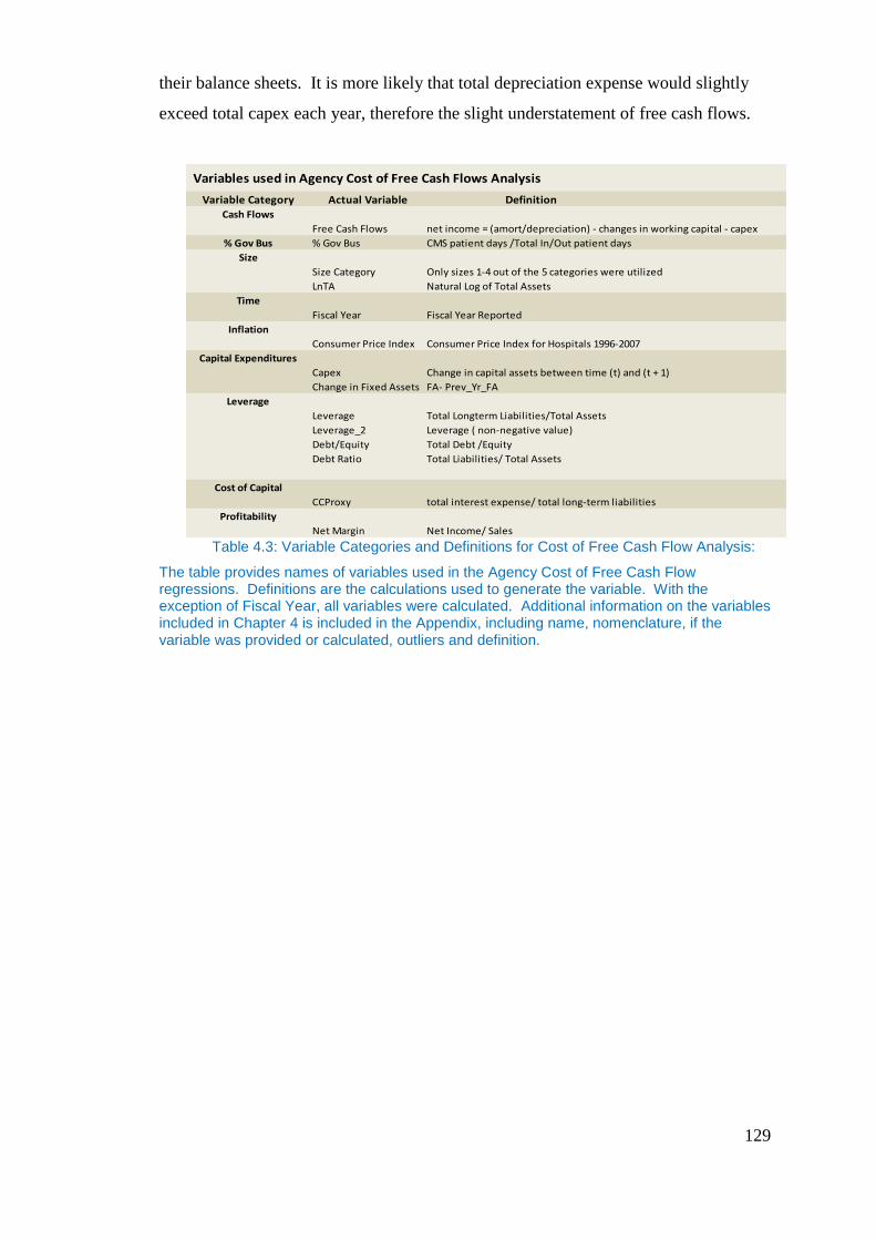
129
their balance sheets. It is more likely that total depreciation expense would slightly
exceed total capex each year, therefore the slight understatement of free cash flows.
Table 4.3: Variable Categories and Definitions for Cost of Free Cash Flow Analysis:
The table provides names of variables used in the Agency Cost of Free Cash Flow regressions. Definitions are the calculations used to generate the variable. With the exception of Fiscal Year, all variables were calculated. Additional information on the variables included in Chapter 4 is included in the Appendix, including name, nomenclature, if the variable was provided or calculated, outliers and definition.
Variables used in Agency Cost of Free Cash Flows Analysis
Variable Category Actual Variable DefinitionCash Flows
Free Cash Flows net income = (amort/depreciation) - changes in working capital - capex
% Gov Bus % Gov Bus CMS patient days /Total In/Out patient days
Size
Size Category Only sizes 1-4 out of the 5 categories were utilized
LnTA Natural Log of Total Assets
Time
Fiscal Year Fiscal Year Reported
Inflation
Consumer Price Index Consumer Price Index for Hospitals 1996-2007
Capital Expenditures
Capex Change in capital assets between time (t) and (t + 1)
Change in Fixed Assets FA- Prev_Yr_FA
Leverage
Leverage Total Longterm Liabilities/Total Assets
Leverage_2 Leverage ( non-negative value)
Debt/Equity Total Debt /Equity
Debt Ratio Total Liabilities/ Total Assets
Cost of Capital
CCProxy total interest expense/ total long-term liabilities
Profitability
Net Margin Net Income/ Sales
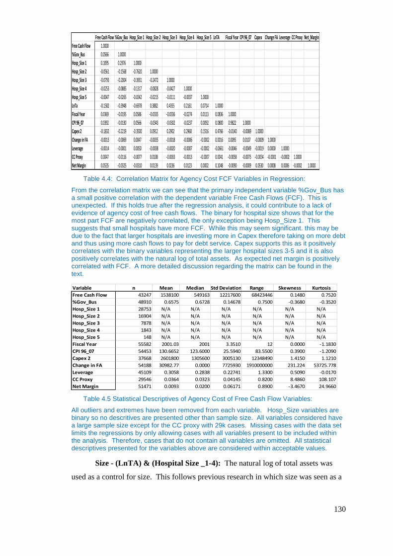
130
Table 4.4: Correlation Matrix for Agency Cost FCF Variables in Regression:
From the correlation matrix we can see that the primary independent variable %Gov_Bus has a small positive correlation with the dependent variable Free Cash Flows (FCF). This is unexpected. If this holds true after the regression analysis, it could contribute to a lack of evidence of agency cost of free cash flows. The binary for hospital size shows that for the most part FCF are negatively correlated, the only exception being Hosp_Size 1. This suggests that small hospitals have more FCF. While this may seem significant. this may be due to the fact that larger hospitals are investing more in Capex therefore taking on more debt and thus using more cash flows to pay for debt service. Capex supports this as it positively correlates with the binary variables representing the larger hospital sizes 3-5 and it is also positively correlates with the natural log of total assets. As expected net margin is positively correlated with FCF. A more detailed discussion regarding the matrix can be found in the text.
Table 4.5 Statistical Descriptives of Agency Cost of Free Cash Flow Variables:
All outliers and extremes have been removed from each variable. Hosp_Size variables are binary so no descritives are presented other than sample size. All variables considered have a large sample size except for the CC proxy with 29k cases. Missing cases with the data set limits the regressions by only allowing cases with all variables present to be included within the analysis. Therefore, cases that do not contain all variables are omitted. All statistical descriptives presented for the variables above are considered within acceptable values.
Size - (LnTA) & (Hospital Size _1-4): The natural log of total assets was
used as a control for size. This follows previous research in which size was seen as a
Free Cash Flow %Gov_Bus Hosp_Size 1 Hosp_Size 2 Hosp_Size 3 Hosp_Size 4 Hosp_Size 5 LnTA Fiscal Year CPI 96_07 Capex Change FA Leverage CC Proxy Net_Margin
Free Cash Flow 1.0000
%Gov_Bus 0.0566 1.0000
Hosp_Size 1 0.1095 0.2976 1.0000
Hosp_Size 2 -0.0561 -0.1568 -0.7620 1.0000
Hosp_Size 3 -0.0793 -0.2004 -0.3931 -0.2472 1.0000
Hosp_Size 4 -0.0253 -0.0885 -0.1317 -0.0828 -0.0427 1.0000
Hosp_Size 5 -0.0047 -0.0265 -0.0342 -0.0215 -0.0111 -0.0037 1.0000
LnTa -0.1582 -0.3948 -0.6978 0.3882 0.4355 0.2161 0.0714 1.0000
Fiscal Year 0.0369 -0.0195 0.0586 -0.0335 -0.0336 -0.0274 0.0113 0.0836 1.0000
CPI 96_07 0.0392 -0.0130 0.0566 -0.0343 -0.0302 -0.0237 0.0092 0.0800 0.9822 1.0000
Capex 2 -0.1832 -0.2219 -0.3500 0.0912 0.2902 0.2960 0.1516 0.4766 -0.0140 -0.0089 1.0000
Change in FA -0.0013 -0.0069 0.0047 -0.0035 -0.0018 -0.0006 -0.0002 0.0016 0.0095 0.0107 -0.0009 1.0000
Leverage -0.0014 -0.0001 0.0050 -0.0038 -0.0020 -0.0007 -0.0002 -0.0661 -0.0046 -0.0049 -0.0019 0.0000 1.0000
CC Proxy 0.0047 -0.0116 -0.0077 0.0108 -0.0033 -0.0013 -0.0007 0.0041 -0.0058 -0.0075 -0.0034 -0.0001 -0.0002 1.0000
Net Margin 0.0535 -0.0325 -0.0310 0.0139 0.0236 0.0123 0.0002 0.1048 -0.0090 -0.0009 0.0530 0.0008 0.0006 -0.0002 1.0000
Variable n Mean Median Std Deviation Range Skewness Kurtosis
Free Cash Flow 43247 1538100 549163 12217600 68423446 0.1480 0.7520
%Gov_Bus 48910 0.6575 0.6728 0.14678 0.7500 -0.3680 -0.3520
Hosp_Size 1 28753 N/A N/A N/A N/A N/A N/A
Hosp_Size 2 16904 N/A N/A N/A N/A N/A N/A
Hosp_Size 3 7878 N/A N/A N/A N/A N/A N/A
Hosp_Size 4 1843 N/A N/A N/A N/A N/A N/A
Hosp_Size 5 148 N/A N/A N/A N/A N/A N/A
Fiscal Year 55582 2001.03 2001 3.3510 12 0.0000 -1.1830
CPI 96_07 54453 130.6652 123.6000 25.5940 83.5500 0.3900 -1.2090
Capex 2 37668 2601800 1305600 3005130 12348490 1.4150 1.1210
Change in FA 54188 30982.77 0.0000 7725930 1910000000 231.224 53725.778
Leverage 45109 0.3058 0.2838 0.22741 1.3300 0.5090 -0.0170
CC Proxy 29546 0.0364 0.0323 0.04145 0.8200 8.4860 108.107
Net Margin 51471 0.0093 0.0200 0.06171 0.8900 -3.4670 24.9660

131
modifying factor in the agency attributes and unit characteristics. In particular, the
size variable takes into account the production capability of the ACH when looking at
FCFs in relation to %Gov_Bus. Total Assets is a variable provided within the MCR.
In addition, a binary variable was created from the size categories described in
Chapter 3. Hospital Size_1-4 was a categorical binary set of dummy variables used to
differentiate the size of the ACH by physical size. Category 5 was excluded from the
binary set so as to avoid over-fitting the model. A value of one was given to cases
that were in the size category, and a zero given to those cases not in the category.
This variable allowed the research to take into account the size of the ACH by bed
size. The size should be positively correlated to free cash flows, as FCF is the actual
value of free cash flows. One would expect that larger ACHs generate larger free
cash flows. The positive correlation of size and free cash flows however is not
supported by the correlation matrix in Table 4.3. In all instances of the size variable
except hospital size one; there is a slight negative correlation with FCF. This is most
likely due to inefficient use of assets to generate FCF. However, no variable is
included in the regression that takes this into account. The correlation of these
variables may be distorted by underlying variables, which would only come to light in
the regression when additional control variables are considered. There is a limitation
in using a binary size variable based upon bed size, as licensed beds listed within the
MCR may not accurately indicate the actual numbers of beds in service to produce
revenues. However this is compensated as ACHs can quickly put these beds in to
operations should demand require it.
Time - (Fiscal Year): The fiscal year was the control for time and was used
to reduce temporal effects within the model caused by time. The expectation was that
this variable in the study would correlate positively with the dependent variable FCF,
and should increase due to the inflation of reimbursement and the inflation of
healthcare cost over the course of this study. This relationship is supported by initial
evidence in Table 4.3.
However, time is a linear construct, and its inclusion within the model did
not completely account for inflation, so a Consumer Price Index (CPI) inflator was
also used. The CPI control, while increasing, does not increase at the same rate each
year, and thus is a better control for inflation within the model, as inflation is a non-
132
linear construct. The combination of time and CPI should work in tandem with the
model to improve explanatory power
Inflation (CPI): The CPI for hospital services was used to control for
inflation within the model, and was only available from 1996 onward. All regression
with CPI as a control was limited to 1996-2007 (U.S. Bureau of Labor Statistics
2009). Inflation is an important variable to be considered within this research as
healthcare inflation has increased at a greater rate for healthcare services than that of
inflation for general products in the U.S. Economy (Jonas, 2007).This variable should
correlate positively with the dependent variable of FCF, as the CPI for hospital
services increases year on year. This relationship has initial confirmation via the
correlation matrix in Table 4.3., where there is a slight positive correlation of 0.0369.
While the CPI control variable controls for inflation, it should increase at a non-linear
rate each year, corresponding to the increases in the FCF due to inflation.
Capital expense - (CAPEX), (Change in FA): CAPEX and change in fixed
assets (FA) were used as the control mechanisms for the uses of free cash flow and
leverage in acquiring assets. Increases in CAPEX and positive changes in FA can lead
to increases in leverage. The FCFs used for acquiring new assets caused FCFs to
decrease. This allowed the model to account for ACH free cash flow in light of
capital spending. CAPEX is a calculated variable that represents the change between
capital assets at time (t) and capital assets at time (t -1). Change in FA is a calculated
variable created using the change in Fixed Assets from the previous year. CAPEX
should deliver a negative relationship with free cash flows overall, because the
calculation of FCF removes CAPEX, so as CAPEX increases, the FCF should
decrease. This relationship is initially confirmed by the relationship in Table 4.3,
however this relationship may change in the regression due to the presence of other
control variables. The use of this variable is somewhat compromised and limited by
the number of ACHs, which recorded total capital expenditures. So Change in FA is
expected to provide a better estimator as fewer cases will need to be ommitted.
Leverage - (Leverage2): Leverage was used to control for size of debt in
relation to the assets in place of the institution. Controlling for leverage takes into
account how differences in ACHs capital structures affect FCF. For instance the
greater the leverage the less FCF as FCF must be used to pay for debt coverage and
therefore would reduce the amount of FCFs. Leverage is one of the key
133
considerations in the agency model as it is proposed that the government seeks to
control overinvestment in healthcare by reducing FCF which , as suggest by Calem
and Rizzo 1995, would reduce access to debt markets and thus reduce the leverage of
the ACH. Leverage_2 was calculated as Total Long-term Liabilities/Total Assets.
Leverage in the study was defined to be a non-negative number, so any negative
values were omitted from the study. Leverage was expected to have a negative
correlation to the FCF, as the FCF is derived after cash flows have been used to
service debt obligations. Therefore, as leverage increases, the amount of cash flow
utilized to service debt increases, reducing the amount of FCF.
Cost of Capital- (CCProxy): CCProxy was used in the study to control for
the cost of capital associated with the amount of debt used by ACHs. The study
assumed that firms with similar debt sizes would differentiate themselves in free cash
flows due to the different costs of capital associated with the debt. The addition of a
cost of capital proxy extends the role of the leverage variable in explaining FCFs of
ACHs as ACHs with higher cost of capital would incur greater interest fees associated
with a given level of debt. Inclusion of this variable allows the model to consider all
levels of credit for ACHs. A proxy was created by taking the total interest expense as
a ratio to total long-term liabilities. The proxy actually measured the cost of debt for
the ACH; however, the cost of debt and the cost of capital were correlated positively,
which allows the use of cost of debt as the proxy. In addition, ACHs are leveraged
heavily; therefore, the bulk of their capital funding is via debt. By measuring the cost
of debt, the model accounted for a great portion of the cost of capital. Limitation in
the use of this proxy was the possibility that some of the long-term liabilities carried
on the balance sheet did not require interest to be paid. In cases where this was true, it
caused the cost of capital to be understated. One would expect that similar to
leverage, the cost of capital would correlate negatively to FCF. The basis for this is
that the FCF is computed after payments for servicing debt.
Profitability - (Net Margin): Net Margin was used as a control within the
study to take into account the variability of generating FCF. Net Margin is an
important variable as it indicates the size of net income in comparison to total
revenues. Net income is the primary variable in the calculation of FCF. As is such
net income the primary driver in the Net Margin ratio, affects the ability to generate
FCF. Net Margin is meant to provide a control for the variance in production of Net

134
Margin and consequently FCF of ACHs. Net Margin should correlate positively with
the FCF in the model, because an ACH that is more profitable should generate more
free cash flows. One might be concerned that Net Margin and FCF are endogenous;
however, the correlation matrix in Table 4.3 indicates that Net Margin and FCF are
only slightly positively correlated. Net Margin was calculated by taking the net
income/total revenue.
Additional information on the variables included in Chapter 4 is included in
the Appendix, including name, nomenclature, if the variable was provided or
calculated, outliers and definition.
4.4 Models
4.4.1 Overview
Two panel data regression models to test for the presence of agency effects in
the presence of the principal-agent relationship were proposed. As discussed
previously, this research looked at two separate agency relationship effects: 1)
signaling via debt; and 2) agency cost of free cash flows. Through these two effects,
the research searched for the presence of agency within the ACH market and the
relationship of agency and capital structure.
4.4.2 Signalling
The premise of signaling within the ACH market put forth within this research
would suggest that signaling is present if the amount of leverage that an ACH carries
positively correlates with the percentage of government business present for that
ACH. In other words, the act of signaling with increased leverage shows better
compliance and greater prudence by management of ACHs due to third-party
monitoring; thus, we would expect a positive correlation of leverage and the
percentage of government business, as government would choose more
efficient/compliant firms. This leads to the following hypothesis:

135
Hypothesis 4-1: Signaling Hypothesis
We reject the null hypothesis if a significantly positive relation is found between
%Gov_Bus and Leverage... ( ) is positive.
Signaling was analyzed via the following relationship in Equation 4-1:
Equation 4-1: Signaling Equation
The model consists of conducting a random effects panel data regression on 13
years of ACH financial data to provide evidence of signaling. Random effects allow
the regression coefficient to be driven by variation over time within each ACH. The
signaling equation examines the relationship between the percentage of revenues
derived from government payors (%Gov_Bus) and the amount of debt of the ACH
(Leverage). The equation contains no instrumental variables.
The primary dependent variable %Gov_Bus denotes the amount of business of
an ACH consumed by the government as a percentage of total business measured in
patient days. Leverage is represented by one of the leverage ratios discussed in
Section 4.3.2.1. The primary independent variable leverage ratio alternates between
Leverage, Leverage_2 (non-negative leverage), Debt to Equity, and the Debt Ratio.
The alternation of the leverage variable allows for different calculations of leverage to
be considered within the research. A dispersion of leverage may be caused by
136
changes in capital expenditure policy of the ACH, free cash flows, growth rate, bank
covenants, and market opportunity.
All of the control variables have been included to capture the operating
characteristics of the ACH. Profitability is defined in Section 4.3.2.1 as the net
margin of the ACH (net income/sales). The inclusion of profitability is to control for
profitability of the ACH in the model, as fluctuations in profitability may affect the
ability of the ACH to leverage, and the government may seek more profitable or less
profitable ACHs depending on policy. Dispersion of the profitability variable may be
caused by reimbursement, patient volume, operating costs, changes in tax policy,
patient mix, and payor mix. Cash flows denote cash flows of the ACH. Cash flows
are defined as free cash flows + capex; as such, any changes in either underlying
variable will cause dispersion. The variable of Cash flows is to control for free cash
flows of the ACH and account for capex. Excess cash flows may lead to investment
in negative NPV projects. Liquidity denotes the liquidity of the ACH-measured ratio
of current assets to total assets. Liquidity affects capex capability of the ACH, which
affects leverage. The government may consider ACHs with greater liquidity more
likely to invest in negative NPV projects. Variance or dispersion of the liquidity
variable may be caused by any changes in current assets or total assets. Size denotes
the size of the ACH, represented as the natural log of total assets of the ACH. Time
denotes the annual period of the study, represented as the fiscal year reported of the
CMS cost report.
denotes the error term. In this case, the error term is comprised of issues
such as the national budget for CMS, the patient mix (the acuity of patients), aging of
the population (older people require more ACH services), health policy shifts, and
changes to the geometric length of stay.
4.4.3 Agency Cost of Free Cash Flows (FCF):
This research suggests that the presence of agency cost of free cash flows in
the U.S. healthcare market is between the government (principal) and ACHs (agent).
The research has suggested that the government is trying to limit overinvestment by
the ACHs, compensate for an inability to monitor the agents output and thus a
inability to form a complete contract due to the market structure, by reducing
137
reimbursement to ACHs. While some may suggest that, the lower reimbursement for
healthcare services has nothing to do with agency problems, but is merely just a
typical market behavior where the consumer wants to achieve the best price. In this
case, the government just wants the best price for purchased services. However,
evidence suggests that the government is trying to solve issues of agency through its
reimbursement strategies (Eldridge and Palmer 2008; McLean 1989; Lee and Zenios
2007;Schneider and Mathios 2006; Conrad and Perry 2009; Melnick 1999). Evidence
of this is provided by changes in reimbursement, post the time frame of this study
(2008). 6 Examples include evidence based reimbursement to pay for outcomes based
upon quality of care, avoidance of perverse incentives to avoid unintended
consequences for ACHs, and to increase transparency in the delivery of care that will
improve quality that leads to moderate cost growth (Trude et.al, 2006, Rosenthal,
2007, Diamond and Kaul, 2009).
Therefore, if we assume that the government is trying to control for agency
problems via its reimbursement strategy we would expect that as the level of
consumption by the government of health services for an individual hospital
increases, the less free cash flows available to ACH, thereby limiting overinvestment
by the restriction in free cash flows. It is from this premise that Hypothesis 4-2 is
derived. The null hypothesis is that there is no significant relation between the
amount of government business and the free cash flows of an ACH, or there is a
significant positive relation between the amount of government business and an
ACHs free cash flows. However, if there is a significant negative relationship between
the percentage of government business and the free cash flows of ACHs, then the null
hypothesis in Hypothesis 4-2 can be rejected, providing evidence of agency cost of
free cash flows.
6 Congress order the Secretary of Health and Human Services in 20005, (which runs CMS) to
change reimbursement methodologies to reduce perverse incentives for ACHs which caused increased
cost of healthcare due to poor delivery which included preventable secondary health conditions created
while in hospital. An example would be nosocomial infections.
138
Hypothesis 4-2: Agency Cost of Free Cash Flows
We can reject the null hypothesis if we find a statistically significant negative
relationship existing between the FCF and % Gov_Bus... ( ) is negative in
Equation 4-2.
Agency cost of free cash flow was analyzed by observing the following linear
regression model expressed in Equation 4-2:
Equation 4-2: Agency Cost of Free Cash Flow
The linear regression model present in Equation 4-2, above, is used to analyze
the correlation and magnitude of such between free cash flows and the percentage of
government business while taking into account inflation, capital expenditures, the
debt of the ACH, the cost of capital paid on such outstanding debt, the profitability of
the ACH, the size of the ACH, and any effect time might have on the model. The
model consist of a random effects panel data regression on 13 years of ACHs’
financial data to determine if there is sufficient evidence to support the presence of
agency cost of free cash flows. The model examines the relationship of ACH free
139
cash flows and the percentage of government business (%Gov_Bus). The regression
contains no instrumental variables.
The dependent variable free cash flows denotes the amount of free cash flows
for the ACH using the definition provides in Section 4.3.2.1. The primary
independent variable %Gov_Bus represents the percentage of government business of
an ACH’s total revenue measured in patient days. Dispersion of the primary
independent variable can be caused by policy shifts, reimbursement changes for
procedures, changes in the GMLOS (geometric length of stay), and/or variation in the
acuity of patients covered by government programs.
All of the control variables included within the regression are included to
provide controls for the operating and financial characteristics of the ACH. Inflation
is represented by use of the CPI for health services and is included in the regression to
correct for changes in both reimbursement and free cash flows that may be derived
from inflationary influences. A capital expenditure variable is included to provided
control for capex policies and trends within the ACH, as these influence the FCF of
the ACH. Leverage was included within the model to control for the use of external
debt financing. As the debt of an ACH increases, more of the ACHs cash flows are
used to support repayment of principal and interest. This is combined with a proxy
for the cost of capital. Cost of capital proxy is included to control for variation in
FCFs due to higher or lower cost of debt. A definition for the cost of capital proxy
can be found in Section 4.3.2.1.
Profitability of the ACH has an influence on the amount of FCF, as ACHs
with higher profitability normally have higher free cash flows. Profitability has been
defined in the previous section on signaling as well as in Section 4.3.2.1. Size is
controlled for in the model, as larger ACHs usually have larger FCFs, and vice versa.
Size is controlled for using a binary categorical variable with the five categories used
in Chapter 3. Time is controlled for using the fiscal year in which the financials were
filed.
(the error term) is comprised of issues such as volume of patient, physician
practice patterns (some physicians order more test than others), cost of labor and
efficiency of the ACH with its assets and its human capital, acuity of the patients in
any given year, and external pricing pressures by the open market. In light of agency
theory, one would expect a negative correlation between the percentage of

140
government business (%Gov_Bus) and the FCF, given the control variables. In other
words, more government business would harm the amount free cash flows an ACH
would be able to generate. The null hypothesis is that there is no relationship or a
positive relationship between %Gov_Bus and free cash flows.
4.5 Results
4.5.1 Signalling:
Several variations of the model were built based on the different definitions of
Leverage that were discussed earlier and the number of control variables. All
regressions were performed at the 95% confidence level. No outliers were removed,
except in the utilization of leverage_2, which removed all negative values for the
leverage variable. The results are presented in Table 4.3.
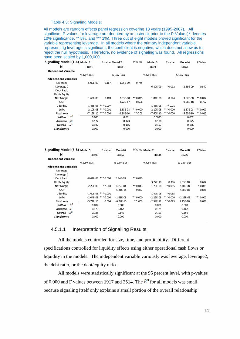
141
Table 4.3: Signaling Models:
All models are random effects panel regression covering 13 years (1995-2007). All significant P-values for leverage are denoted by an asterisk prior to the P-Value ( * denotes 10% significance, ** 5%, and *** 1%). Three out of eight models proved significant for the variable representing leverage. In all models where the primary independent variable representing leverage is significant, the coefficient is negative, which does not allow us to reject the null hypothesis. Therefore, no evidence of signaling was found. All regressions have been scaled by 1,000,000.
4.5.1.1 Interpretation of Signalling Results
All the models controlled for size, time, and profitability. Different
specifications controlled for liquidity effects using either operational cash flows or
liquidity in the models. The independent variable variously was leverage, leverage2,
the debt ratio, or the debt/equity ratio.
All models were statistically significant at the 95 percent level, with p-values
of 0.000 and F values between 1917 and 2514. The for all models was small
because signaling itself only explains a small portion of the overall relationship
Signalling Model (1-4) Model 1 P Value Model 2 P Value Model 3 P Value Model 4 P Value
N 38761 31888 38273 31462
Dependent Variable % Gov_Bus % Gov_Bus % Gov_Bus % Gov_Bus
Independent VariablesLeverage -5.09E-09 0.167 -1.25E-09 0.745
Leverage 2 -6.80E-09 * 0.092 -2.59E-09 0.542
Debt Ratio
Debt/ Equity
Net Margin 1.63E-08 0.189 3.53E-08 ** 0.025 1.84E-08 0.144 3.82E-08 ** 0.017
OCF -1.72E-17 0.606 -9.96E-18 0.767
Liduidity -1.48E-08 *** 0.007 -1.45E-08 ** 0.01
LnTA -2.10E-08 *** 0.001 -2.33E-08 *** 0.000 -2.12E-08 *** 0.000 -2.37E-08 *** 0.000
Fiscal Year -7.15E-10 *** 0.000 -4.88E-10 ** 0.03 -7.60E-10 *** 0.000 -5.53E-10 ** 0.015
Within 0.003 0.001 0.0033 0.002
Between 0.177 0.173 0.178 0.175
Overall 0.197 0.166 0.197 0.166
Significance 0.000 0.000 0.000 0.000
Signalling Model (5-8) Model 5 P Value Model 6 P Value Model 7 P Value Model 8 P Value
N 43909 37052 36145 30229
Dependent Variable % Gov_Bus % Gov_Bus % Gov_Bus % Gov_Bus
Independent VariablesLeverage
Leverage 2
Debt Ratio -8.62E-09 *** 0.000 5.84E-09 ** 0.015
Debt/ Equity 3.27E-10 0.366 5.03E-10 0.694
Net Margin 2.25E-08 **.040 2.65E-08 ** 0.043 1.78E-08 * 0.055 2.48E-08 * 0.089
OCF -5.31E-18 0.867 7.38E-18 0.826
Liduidity -1.60E-08 *** 0.001 1.47E-08 * 0.055
LnTA -2.04E-08 *** 0.000 -1.68E-08 *** 0.000 -2.22E-08 *** 0.000 -2.22E-08 *** 0.000
Fiscal Year -5.77E-10 0.004 -6.74E-10 ** .003 -2.54E-11 ** 0.025 1.15E-10 0.621
Within 0.002 0.006 0.001 0.000
Between 0.173 0.162 0.174 0.162
Overall 0.185 0.149 0.193 0.156
Significance 0.000 0.000 0.000 0.000
142
between government business and the amount of leverage of ACHs. The debt
variable was significant in Models 3, 5, and 6, with p-values ranging from 0.000 to
0.092. Where debt was significant, the coefficients were negative. On the other hand,
the liquidity variable was the better control compared to operational cash flows
(OCF), which was insignificant in all of the models. In models in which only the
liquidity variable was changed, was lower for operational cash flows. Although
Models 3, 5, and 6 were significant for the primary independent explanatory variable,
the negative beta for Leverage did not allow us to reject the null hypothesis.
Therefore, no evidence of signaling was found.
In all of the cases where the Leverage was significant, the explanatory variable
was negative. This suggested a very small negative relationship with % Gov_Bus.
Although not in line with the signaling hypothesis put forward within this research,
these findings were consistent with that of Calem and Rizzo (1995), suggesting that
agency costs of debt may limit investment when firms depend on the availability of
internal funds. In this case, ACHs may be restricted in their access to debt markets
by reduced FCFs. In other words, the liquidity of the firm is determining access to
debt markets because the FCF must be promised in the future to service debt. Calem
and Rizzo (1995) suggested that limits on payments to ACHs affect liquidity, and thus
limit their ability to acquire financing. There is an additional possibility that ACHs
are using the stability in cash flows from government to replace investments
purchased via debt by using pay-as-you-go strategies utilizing excess free cash flows.
However, if there is evidence of agency cost of FCFs, this would be unlikely.
Further research on signaling theory is suggested, as other factors may have
affected the results. Other distortions within the data or other countermanding forces
within the market that are not accounted for within this study may be restricting
signaling, such as noisy or inconsistent data, which was unrecognized and
unaccounted for in the data preparation or the methodologies used in the signaling
models. There also may be variables that would have improved the regression results,
but were either unavailable or unknown. Measurement errors or human mistakes
entering the data by CMS also could have skewed the results. In addition, agency
cost of free cash flows may be interfering with the ACHs’ ability to signal, as
reduction in free cash flows may limit firm access to debt markets.

143
4.5.2 Agency Cost of Free Cash Flows
Several different models were used in order to take into account the different
explanatory power of the primary independent, dependent, and the control variables.
Random effects linear regression was utilized to examine the relationship of FCF to
%Gov_Bus for each model. All the control variables account for size, time, and
inflation. Other control variables were added in subsequent models.
Eight different specifications of the model were used to provide evidence of
the agency cost of free cash flows. The core model, which accounts for the primary
independent variable, % Gov_Bus, also controlled for size and time. Seven
additional control variables were added on the core model. Each subsequent control
variable was added one at a time into the model, creating a total of eight models
overall. All eight models removed the outliers for the FCF, the dependent variable.
The approximate (n) for all eight models ranged from 33,324 on the low end to
38,860 on the high end. Total (N) for the population was 55,582. Losses of cases
were the result of system missing values within the dependent, independent, and
control variables. The majority of cases were lost due to the removal of outliers for
the FCF. As control variables were included, the (n) for those models dropped as a
result of system missing data.
The results of the models are presented in Table 4.4. The models were ordered
by the number of control variables used in the first model, and additional control
variables were added in each subsequent model. The primary driver for adding
additional control variables was to increase the explanatory power of the model. Each
variable added additional explanatory power as the increased with each model,
with a low of 0.026 for the first model, and an of 0.056 for the eighth model.
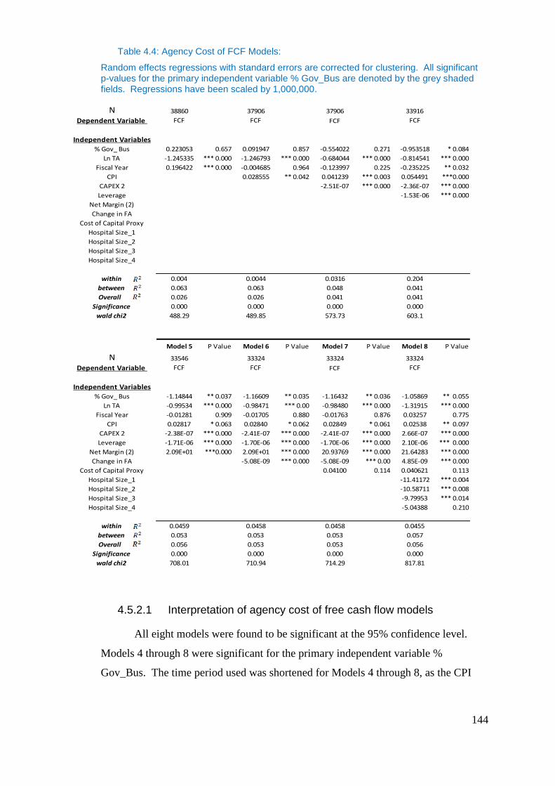
144
Table 4.4: Agency Cost of FCF Models:
Random effects regressions with standard errors are corrected for clustering. All significant p-values for the primary independent variable % Gov_Bus are denoted by the grey shaded fields. Regressions have been scaled by 1,000,000.
4.5.2.1 Interpretation of agency cost of free cash flow models
All eight models were found to be significant at the 95% confidence level.
Models 4 through 8 were significant for the primary independent variable %
Gov_Bus. The time period used was shortened for Models 4 through 8, as the CPI
N 38860 37906 37906 33916
Dependent Variable FCF FCF FCF FCF
Independent Variables
% Gov_ Bus 0.223053 0.657 0.091947 0.857 -0.554022 0.271 -0.953518 * 0.084
Ln TA -1.245335 *** 0.000 -1.246793 *** 0.000 -0.684044 *** 0.000 -0.814541 *** 0.000
Fiscal Year 0.196422 *** 0.000 -0.004685 0.964 -0.123997 0.225 -0.235225 ** 0.032
CPI 0.028555 ** 0.042 0.041239 *** 0.003 0.054491 ***0.000
CAPEX 2 -2.51E-07 *** 0.000 -2.36E-07 *** 0.000
Leverage -1.53E-06 *** 0.000
Net Margin (2)
Change in FA
Cost of Capital Proxy
Hospital Size_1
Hospital Size_2
Hospital Size_3
Hospital Size_4
within 0.004 0.0044 0.0316 0.204
between 0.063 0.063 0.048 0.041
Overall 0.026 0.026 0.041 0.041
Significance 0.000 0.000 0.000 0.000
wald chi2 488.29 489.85 573.73 603.1
Model 5 P Value Model 6 P Value Model 7 P Value Model 8 P Value
N 33546 33324 33324 33324
Dependent Variable FCF FCF FCF FCF
Independent Variables
% Gov_ Bus -1.14844 ** 0.037 -1.16609 ** 0.035 -1.16432 ** 0.036 -1.05869 ** 0.055
Ln TA -0.99534 *** 0.000 -0.98471 *** 0.00 -0.98480 *** 0.000 -1.31915 *** 0.000
Fiscal Year -0.01281 0.909 -0.01705 0.880 -0.01763 0.876 0.03257 0.775
CPI 0.02817 * 0.063 0.02840 * 0.062 0.02849 * 0.061 0.02538 ** 0.097
CAPEX 2 -2.38E-07 *** 0.000 -2.41E-07 *** 0.000 -2.41E-07 *** 0.000 2.66E-07 *** 0.000
Leverage -1.71E-06 *** 0.000 -1.70E-06 *** 0.000 -1.70E-06 *** 0.000 2.10E-06 *** 0.000
Net Margin (2) 2.09E+01 ***0.000 2.09E+01 *** 0.000 20.93769 *** 0.000 21.64283 *** 0.000
Change in FA -5.08E-09 *** 0.000 -5.08E-09 *** 0.00 4.85E-09 *** 0.000
Cost of Capital Proxy 0.04100 0.114 0.040621 0.113
Hospital Size_1 -11.41172 *** 0.004
Hospital Size_2 -10.58711 *** 0.008
Hospital Size_3 -9.79953 *** 0.014
Hospital Size_4 -5.04388 0.210
within 0.0459 0.0458 0.0458 0.0455
between 0.053 0.053 0.053 0.057
Overall 0.056 0.053 0.053 0.056
Significance 0.000 0.000 0.000 0.000
wald chi2 708.01 710.94 714.29 817.81

145
was the limiting control variable, and only the years 1996-2007 were used. The
reduction was due to a limitation in the CPI for hospital services; the series lacked
information for the year 1995. While the generalized CPI would have been available
for use in modeling, it was decided that it would be more appropriate to use a CPI for
hospital services, which allowed a more precise measurement of inflation in relation
to the cash flows studied. This meant reducing the period of the study by one year
when including the inflation variable as a control. Models1, 2, and 3 proved not to be
significant for the primary independent variable %Gov_Bus. This primarily is driven
by the lack of explanatory variables within these models.
Model 1 only controlled for size and time in addition to the primary
independent variable. A sample size of 38,860 cases was included in the regression.
The adjusted for Model 1 was 0.026, or 2.6%. The control variables for size and
time remain significant within the model with P-Values of 0.000.
Model 2 provided an of 0.026; however, it was not significant for
%Gov_Bus, the primary independent variable. Only the natural log of total assets
remained significant within the model, with a P-Value of 0.000; all other variables
were insignificant. Model 2 was insignificant most likely because of the lack of free
cash flow explanatory variables. This was confirmed, as the between Model 1 and
Model 2 remained unchanged.
Model 3 added Capex as an explanatory variable to account for capital
expenditures’ affect upon free cash flows. Inclusion of this variable increased the
from 0.026 to 0.041. The primary independent variable (%Gov_Bus) remained
insignificant within the model; however, the sign was negative. The most likely cause
was the lack of additional explanatory variables for free cash flows in the model.
Model 4 with an overall of 0.041 provided the smallest explanatory power
for a model in which the primary independent variable %Gov_Bus was significant.
Model 4 controlled for size, time, inflation, capital expenditure, and leverage. The
%Gov_Bus variable beta coefficient was -0.952518 with a P-value of 0.084, and a
model significance of 0.000. The inclusion of leverage as a control variable improved
the performance of the primary independent variable % Gov_Bus, changing the P-
Value to significant in the process from 0.271 in the previous model, to 0.084 at a 10
percent significance level. The negative correlation presented in the beta for
146
%Gov_Bus suggests that there is a negative relationship between FCF and the
percentage of government business derived by an ACH.
This model suggested that for every percentage increase in government
business, an ACH would lose $953,518 in free cash flows. This supports the theory
of agency cost of free cash flows presented within this research. Natural log of total
assets (LnTA) was significant as well for the model, with a P-Value of 0.000. The
beta presented for LnTA was -0.814541. The beta presented for LnTA was not in line
with the expectations of the research. This suggested that larger ACHs have less free
cash flows, and that larger hospitals overinvest more than smaller ones. This follows
Parrino and Weisbach (1999), who suggested that firms with large FCF and little
growth opportunities have a greater propensity to overinvest. This also is in line with
Nahata (2005) and Glied (2003), who stated that ACHs in highly competitive markets
spend more on capital investments, and therefore a have lower FCF. Larger hospitals
would be located in more competitive markets, as they generally are found in larger
urban centers with multiple hospitals.
Fiscal year was significant, with a P-Value of 0.032. It should be noted that
the beta coefficient was negative, with a value of -0.235224. This suggested that as
each year progresses, the FCFs decrease by $235,224.50, which perhaps would
suggest that reductions in reimbursement over time are having an effect on ACHs. As
expected, the variable CPI was significant with a P-Value of 0.000. The beta value
of 0.054491 confirmed the positive correlation with the FCFs, as expected. Capex
had a negative correlation with the FCFs. Capex was significant with a P-Value of
0.000 and a beta of -2.36E-07. Capex was expected to have a negative relationship,
and results are in line with expectations, as it should reduce the FCFs. Leverage was
significant with a P-value of 0.000, and presented a negative beta of -1.53E-06. This
was also in line with expectations, as an increase in leverage should increase
borrowing costs, which decreases the FCFs.
Model 5 increased to 0.056, an increase of 0.015, or 1.5%. Model 5
controlled for the same variables as Model 4, plus the additional control variable of
profitability via the variable Net Margin. The beta for %Gov_Bus variable was -
1.148436 similar to Model 4, and had a P-value of .036. Model 5 was significant with
a value of .000. The large negative beta for %Gov_Bus suggested that for every
percent increase in government business by an ACH, the ACH experienced a decrease
147
in the FCFs of $1,148,436. For larger institutions, this may not be of concern;
however, for smaller ACHs, this presents concern, as they are more susceptible to
changes in the FCFs (Calem & Rizzo 1995).
The size variable LnTA remained significant with a P-Value of 0.000, and this
is consistent with Model 4, as the beta remained largely negative at -0.99534. This
continued to suggest that larger ACHs are more likely to overinvest. This is
counterintuitive and goes against the initial expectations outlined previously. Fiscal
Year was not significant within this model. The CPI almost was significant in this
model, with a P-Value of 0.063, and presented a positive beta coefficient, which is in
line with the expectations. Capex was significant with a P-Value of 0.000, and a beta
of -2.38E-07 remained in line with expectations. Leverage was significant with a P-
Value of 0.000, and presented a beta of -1.71E-06, which was in line with
expectations and continued to suggest that as leverage increases, borrowing costs
decrease the FCFs.
Model 6 was significant for the primary independent explanatory variable,
%Gov_Bus, with a P-Value of 0.035 and a negative beta of -1.16609. In this model,
for every percent change in government business, there was a reduction of $1,166,087
in the FCFs. This continued to suggest that government is heavily affecting the FCFs
of ACH. While adding controls for change in fixed assets in addition to controlling
for size, time, inflation, capital expenditure, leverage, and profitability, the
decreased slightly to 0.053. The decrease in explanatory capability of the model was
explained by the change in the fixed assets control variable. The variable was
significant with a P-value of 0.000; however, the change in fixed assets provided less
explanatory capability when added to the model. The size variable LnTA remained
negatively correlated with the FCFs, which continued to support previous models that
suggested that as ACHs get larger in total assets, this negatively affects FCF. The
negative correlation also supported previous concerns of overinvestment or
investment in negative NPV projects. In other words, while ACHs may be adding
additional assets in place, they are not efficient at producing FCFs. This lack of
inefficient use of assets in place suggests that concerns of overinvestment and
investment in allocative inefficient services are valid.
Model 7 added cost of capital to the control variables. The cost of capital
variable was not significant, with a P-value of 0.114, and does not improve the
148
explanatory power of the model. The remained at 0.053 and was significant at
0.000. The primary independent variable %Gov_Bus had a value -1.16432 and a P-
value of 0.036. For every increase in the percentage of government business, an ACH
experienced a decrease in FCFs of $1,164,322. These results continued to support the
presence of agency costs of free cash flows within the U.S. healthcare market. The
lack of change in the was due to the insignificance of cost of capital to the model.
The LnTA was significant, with a P-Value of 0.000, and continued to support
negative correlation with the FCFs with a beta of -0.98480. This beta continued to
suggest that increases in total assets negatively affect FCFs. Overinvestment by
ACHs and investment in negative NPV projects or allocative inefficient services has
been suggested as the underlying cause for agency cost of free cash flows, and these
results confirmed the premise that larger hospitals overinvest more than smaller ones..
Model 8 added four binary variables to control for size. While five categories
were discussed in Chapter 3, only four binaries were included to minimize over-fitting
the model (n-1). The model presented an overall which was computed at 0.056,
and %Gov_Bus was significant, with a P-Value of 0.018, and a negative beta
coefficient of -1.05869 For every 1% increase in the percentage of government
business, free cash flows decreased by $1,058,690.00. The LnTA remained
significant within the model, with a P-Value of 0.000. The coefficient for the LnTA
was highly negative at -1.1915. The beta value continued to support the
overinvestment problems of larger ACHs, or ACHs investing in negative NPV
projects.
If this is compared with the other size variable in this regression,
Hospital_Size 2-5, which provided a large negative correlation with the FCFs as well,
one sees that hospital bed size is suggesting that larger hospitals have less free cash
flows. This would further reinforce the results from obtained via LnTA, which
suggest that larger hospitals overinvestment more and invest in allocative inefficient
services, which adds to lower free cash flows. The evidence that LnTA correlates
with bed size and the FCF further supports the overinvestment problem. This
evidence, along with %Gov_Bus negative correlation with the FCFs, further supports
agency cost of free cash flow within the healthcare market.
The value of all models were low. In order to ensure against bias due to
specification error in the estimated coefficients, all data that could be obtained to
149
explain the relationship between percentage of government business and free cash
flows were included as variables. Additional explanatory variables that would have
improved the values were either not available or non-definable. In addition, to
allow for a more efficient model, a random effects panel regression was performed.
Improvement on the regression performed may be possible with a larger dataset that
provides greater explanatory variables to be included.
4.6 Conclusions
The use of agency theory to describe the relationship of payors and providers
of healthcare is well established by previous literature. 7 The research undertaken in
this chapter sought evidence of agency costs of signaling and agency costs of free
cash flows that might be a result of reimbursement schemes or schedules used by the
government insurer, CMS. Payments have long been known to be used to incentivize
agents to align the goals of the agent with those of the principal. Previous research
suggests that payment methodologies are used in healthcare to solve agency problems
created in the principal-agent relationship between payor and provider (Conrad and
Perry 2009; Melnick et al 1999; Peterson et al 2006). Alignment of incentives is
important in healthcare as problems regarding the principal agent relationship are
acute due to the inability of the insurer to monitor output of the provider (McLean
1989).
By analyzing the principal-agent relationship between the government and
ACHs, this chapter investigated evidence of signaling and agency cost of free cash
flows. Both characteristics of agency costs are suggested to exist as a result of the
federal government’s need to monitor ACHs and reduce free cash flows under the
ACHs’ control. The environment in which ACHs operate is skewed by the existence
of a moral hazard on the part of patients, whereby they are not exposed to the
consequence of consumption via price, and therefore make choices to consume based
7The use of Agency Theory in healthcare is supported by the previous research of McLean (1989);
Chalkley and Khalil (2005); Jack (2004); Schneider and Mathios ( 2006); Ryan (1994); and Mooney
and Ryan (1993).
150
on quality or perceived quality. The empirical results extend prior research that
suggested that the presence of moral hazard within the ACH market causes ACHs to
compete on quality or perceived quality as a result (Glied 2003; Newhouse 1981;
Nahata 2005). The presence of the moral hazard within the ACH market is important
as it creates conditions that lead ACHs to overinvest and take on projects that have a
negative NPV or are considered allocative inefficient (Pauly et al. 1986; Gaynor et al.
2000; Wang 1999; Glied 2003; and Nahata 2005).
Glied (2003) made the case that ACHs make some investments in projects that
have little or negative economic worth in order to compete via quality or perception of
quality. Under these conditions, the CMS seeks to monitor ACHs better and therefore
minimize wasteful overinvestment. Adding the agency relationship between the CMS
and ACHs and agency theory indicates the behavioral outcomes of this relationship.
In Chapter 4, two testable hypotheses—signaling and agency cost of free cash
flows—were demonstrated.
The premise of signaling was proposed under the notion that ACHs wish to
indicate efficiency to government through debt in order to avoid lower reimbursement
for health services. Expanding on the premise put forward by Jensen (1986), that debt
can reduce agency costs by lenders acting as a third-party monitor, this research
promotes a premise that ACHs seek to signal compliance with the government and to
signal that ACHs are running efficiently and not choosing negative NPV projects.
Lenders acting as third-party monitors ensure that ACHs are performing with
documented financial loan covenants and are able to repay borrowed capital plus
borrowing costs.
The premise suggests that ACHs with greater amounts of revenues from
government payors will want to signal more, and those with less revenue from the
government will signal less. The reason for such consideration is that due to its long-
term relationship with ACHs, the government will try to reduce overinvestment and
other problems with the agency relationship through changes in reimbursement, a
known methodology used to solve problems of agency and incentivize agent
behavior(Lee and Zenios 2007; Jack 2004; Eggleston 2005). These changes in
151
reimbursement usually negatively affect revenues, and consequently free cash flows;
therefore, ACHs with larger revenue streams at risk will signal more. 8
The testable hypothesis put forward was that the greater the percentage of
revenues derived from the government, the more ACHs will take on debt to signal
their compliance with government wishes. Eight linear regression models for
signaling were created with the percentage of government business as the dependent
variable, and leverage of the ACH as the primary independent variable. Additional
variables controlled for profitability, liquidity, size, and time.
All eight models were significant, with three of the eight significant for
leverage. The significant coefficients for leverage were all negative, indicating a
negative correlation between government and leverage. Therefore, the regression
analysis did not support the signaling premise put forward within this chapter. There
was no positive correlation between the amount of debt within ACHs and the
percentage of government revenues derived by those ACHs. Therefore, no evidence
of signaling was found. The negative correlation may be due to noisy data, or
signaling may be affected by other countermanding forces within the market that
prohibit either a desire or capability by ACHs to signal via debt, such as the agency
cost of free cash flows and or other agency costs.
The second premise in this chapter was that agency cost of free cash flow is
suggested to exist because the government, acting as the principal, wishes to reduce
free cash flows to ACHs in order to inhibit overinvestment or investment in allocative
inefficient services, as well as other abhorrent agent activity. The research indicated
that ACHs are overinvesting due to the presence of moral hazard within the ACH
market, which causes ACHs to compete on quality. The government, seeking to
reduce free cash flows, lowers reimbursements to ACHs, and thus controls the
overinvestment and other agency problems (Peterson et al 2006; Melnick et at 1989;
Conrad and Perry 2009; and Mclean 1989). The argument was constructed using the
8 Penalties have been shown to be more effective in curbing abhorrent agency behavior than
bonuses or additional payments (Conrad and Perry 2009; Kahneman and Tversky 1979; Town et al
2004; Tversky and Kahneman 1986).
152
premise that the more ACHs derive their revenues from government payors, the lower
the free cash flows of the ACH.
The testable hypothesis was that there is a significant negative correlation
between the percentage of government business and the ACHs’ free cash flows. Eight
regression models were created, with ACH free cash flows as the dependent variable,
and percentage of government business as the primary independent variable.
Additional control variables were size, time, CPI, capital expenditure, leverage,
profitability, and cost of capital. Size was controlled via two variables: natural log of
total assets, and four binary variables accounting for hospital bed size.
All eight models were significant; however, only five of the eight were
significant for the primary independent variable Percentage of Government Business.
In all cases of significance, the beta coefficient for %Gov_Bus was highly negative,
suggesting that for every percentage change increase in government business, free
cash flows are likely to suffer anywhere from $953,518 to $1,164,322. The results
supported the presence of agency cost of free cash flows in the ACH market.
Additionally, analyzing the regression models for agency cost of free cash
flows showed that the beta coefficient for the variable for natural log of total assets
was significant and highly negative. The negative correlation of assets and free cash
flows would suggest underperforming or inefficient assets. Typical assets are a
measurement of the production capability of a firm to produce revenues, and
consequently free cash flows, and thus correlate positively; the greater the assets in
place, the greater the revenues. The evidence in the regression models suggested the
presence in larger firms of overinvestment and/or investment in allocative inefficient
services . This confirmed the research of overinvestment and inefficiency (Pauly et
al. 19869; Gaynor et al. 2000
10; Wang 1999
11; and Glied 2003
12).
9 Pauly (1986) argued that large inefficiencies in healthcare were driven by tax subsidies, which
cause more insurance to be acquired. The presence of more insurance within the market removed the
consequence of consumption for patients as well as created perverse incentives for providers, which led
to more costly healthcare on a per patient day basis. Overinvestment was thought to beonetype of the
inefficiencies found.

153
The empirical results provided evidence to supports agency cost of free cash
flows, as five out of eight of the agency cost of free cash flow models showed
significance. The negative beta demonstrated an inverse relationship between free
cash flows and government business. The results indicated that as an ACH increased
the percentage of business derived from government sources, the lower its free cash
flows were. These limitations placed upon the free cash flows of the ACHs have an
adverse effect upon their capital structures. As ACHs have less free cash flows, the
choices of capital structure become limited, as their access to debt markets is
restricted. This restriction of free cash flows and limitation of access to debt markets
causes managers to become dependent on internal funds (Calem and Rizzo 1995).
The reduction in capital structure choices forces ACHs to incur higher opportunity
cost, and thereby ACHs have more selective criteria for new projects.
Based upon the findings within this chapter, signaling is not likely to exist
within the U.S. ACH market. However, the most likely cause is the effect of the
agency cost of free cash flows on the ACH’s ability to signal by limiting free cash
flows. By limiting free cash flows, not only is the government restricting
overinvestment, but also limiting ACHs’ access to debt markets. These findings make
sense as alignment of goals between principal and agents via payments in healthcare
are widely recognized (Peterson et at 2006; Eldridge and Palmer 2009; Melnick et al
10 Gaynor et al (2000) had suggested that moral hazard due to insurance introduces a distortion into
the medical market that requires analysis of the second-best outcome. In the presence of moral hazard
due to health insurance, consumers will demand “too much” medical care ex post. They suggest that
the presence of moral hazard may lead to overinvestment by hospitals. 11
Wang 1999 examined efficiency amongst hospitals and found that larger hospitals were more
inefficient. They suggest that larger hospitals were inefficient due to excess services that were under-
utilized. Underutilization via excess services was promoted in this research to be a form of
overinvestment.
12 Glied (2003) blamed the moral hazard of insurance for creating an environment which created
demand for new healthcare technologies and consequently created demand for healthcare facilities to
purchase these new technologies. She suggests that this maybe exists even though there is not enough
utilization of such resources. The research presented suggests that the demand and purchase of new
technologies by hospitals when underutilized is overinvestment.
154
1989; Conrad and Perry 2009; Lee and Zenios 2007; Jack 2004; and Eggleston 2005).
Furthermore, the findings of this chapter are similar to Calem and Rizzo (1995),
which suggests that payments by insurers have an effect on free cash flows of
hospitals and where hospitals had lower free cash flows this affected their ability to
attain debt or limited their access to debt and made them more dependent on internal
funds for investment. The similarity of these findings also explains why signaling
was not found. As Calem and Rizzo (1995) suggest hospitals with lower free cash
flows are restricted in their ability to obtain debt. ACHs with greater government
business have less free cash flows this makes it difficult for them to have access or
take on additional debt, therefore limiting their ability to signal compliance via debt.
Findings within this research supported previous research that suggested that the
limitation of payment to ACHs impedes their ability to invest, as it restricts cash
flows and cash under management. The restriction of cash flow available to
management limits the ability of the ACH to overinvest (Stulz 1990). While Stulz
(1990) research was applied in a traditional firm perspective it is applicable to the
agency environment described in this research.
The evidence of agency costs of free cash flows in this research suggests that
these costs have an effect on the capital structure of ACHs. The results presented here
confirm the previous findings of McLean (1989), who suggested, “Some of the
supposed unequal access to capital among providers may be a result of differing
degrees of agency costs.” The findings of the current research suggest that the
variation in access to capital could be due to the varying amount of government
business, which has the effect of limiting free cash flows. These limitations following
on from Calem and Rizzo (1995) constrain access to debt markets and thus as
variation in free cash flows occurs, so does access to capital via debt.
Agency costs of free cash flows partially explain McLean’s (1989) statement.
Thus, the presence of agency costs of free cash flows is important for us to understand
fully as it may prohibit ACHs from acquiring new equipment and services, and may
have consequences (e.g. reducing the quality of health care). By constraining the
financial freedom of ACHs may lead to variation in quality of healthcare between
hospitals, as ACHs with greater cash flows would be able to provide better quality
and possibly even better access to newer forms of treatment. This is important to

155
consider, as current policies are concerned with better quality and equal access to
healthcare for all.
156
5. Monopsony in Healthcare and Literature
5.1 Introduction
Monopsony rarely exists in markets. However, when it does exist, it creates
inefficiencies within that market. As a result of monopsony, firms encounter
situations in which financial decisions about their capital structures can be affected.
Previous chapters of this thesis contemplated inefficiencies and tested theories
of firm behavior (with respect to capital structure decisions, agency cost of free cash
flows, and signaling). Using economic theory, this chapter focuses on an alternative
and/or complementary condition within the ACH market, monopsony. Just as Jensen
and Meckling (1976) used agency as a substantial factor in decisions of the firm,
monopsony also affects firm behavior and must be considered as an underlying reason
for management decisions regarding capital structure, especially within the U.S.
healthcare market. This is driven by a legal framework, which allows monopsony to
exist within healthcare, while other markets must comply with traditional
interpretations of the antitrust laws present within the U.S. Taking this point further
there is prior research, which either indicates the possible presence of monopsony or
that it is present within U.S. Healthcare. The purpose of this chapter is to provide a
review of the economic theory of monopsony, antitrust via the Sherman Antitrust Law
and monopsony, and an examination of previous relevant research, in order for the
reader to have a greater understanding of monopsony within healthcare and to
contextualize the empirical research presented in Chapter 6.
This chapter begins with a discussion of monopsony in its traditional form and
compares it with the monopsony structure under the all-or-nothing contract scenario
considered in this research. The construct of monopsony is then examined in the
context of U.S. antitrust law, with an in-depth discussion of how monopsony is able to
exist within the healthcare market. The research then provides an overview of
monopsony literature as it relates to non-healthcare and healthcare contexts, providing
evidence of monopsony of healthcare via prior studies and market relationships. The
discussion presented here, provides a basis for the empirical research conducted later
in Chapter 6 as similar studies present considerations and constructs for the models
used there, including collusive monopsony, the dichotomy of healthcare insurance as

157
two markets, and the misunderstanding of monopsony and its effects on consumer
harm via financial harm to the supplier, as represented by Zerbe(2005).
5.1.1 Theory of Monopsony
Monopsony in a market causes distortion within that market from its efficient
form. The demand side of the market reaps excess economic rents by setting lower
prices for input goods/services than it would in a perfectly competitive market and
ultimately consuming less than if the market was perfectly competitive. The supplier
within the market suffers from lower prices, less consumption, and consequently
lower profit margins and less free cash flow. The traditional model of monopsony
often is used for insight into the allocation of resources and the distribution of income
as a consequence of buyer power. Traditional monopsony assumes the
followingabout the monopsonist and seller of inputs: Sellers are free to determine the
quantity of inputs to supply for a given price; prices paid by the monopsonists are
equal to the marginal cost; and the monopsonist has full knowledge of the industry
supply curve and will use this knowledge of the industry supply curve to leverage
price discounts.
All monopsonists exhibit profit maximizing behavior, thereby seeking to
capture additional rents available within the market. By using knowledge of the
industry supply curve, the monopsonist is able to lower the price paid to the supplier
to the marginal costs of the supplier. This behavior can be seen in the following
description of traditional monopsony. In Figure 5.1, we see that market equilibrium at
Point C where supply equals demand. The supply curve typically answers the
question of what is the quantity of goods that will be supplied at a given price. In this
case, Qc represents the quantity demanded, and Pc represents the market price under
the competitive market equilibrium. Thus, the supplier is choosing to supply
quantities equal to full demand. Under the traditional model of monopsony, the
monosonist forces the supplier to sell at the monopsonist’s price, Pm, which reduces
the quantity supplied at price Pm to quantity Qm.
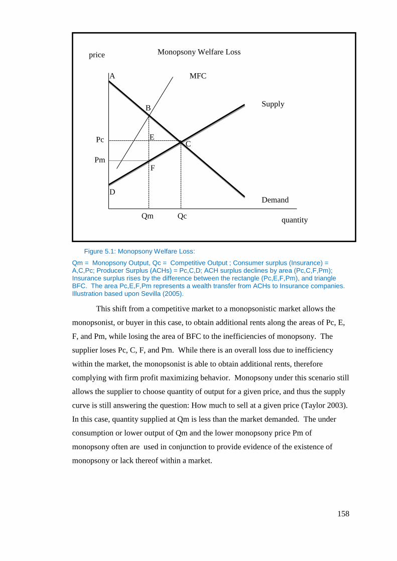
158
Figure 5.1: Monopsony Welfare Loss:
Qm = Monopsony Output, Qc = Competitive Output ; Consumer surplus (Insurance) = A,C,Pc; Producer Surplus (ACHs) = Pc,C,D; ACH surplus declines by area (Pc,C,F,Pm); Insurance surplus rises by the difference between the rectangle (Pc,E,F,Pm), and triangle BFC. The area Pc,E,F,Pm represents a wealth transfer from ACHs to Insurance companies. Illustration based upon Sevilla (2005).
This shift from a competitive market to a monopsonistic market allows the
monopsonist, or buyer in this case, to obtain additional rents along the areas of Pc, E,
F, and Pm, while losing the area of BFC to the inefficiencies of monopsony. The
supplier loses Pc, C, F, and Pm. While there is an overall loss due to inefficiency
within the market, the monopsonist is able to obtain additional rents, therefore
complying with firm profit maximizing behavior. Monopsony under this scenario still
allows the supplier to choose quantity of output for a given price, and thus the supply
curve is still answering the question: How much to sell at a given price (Taylor 2003).
In this case, quantity supplied at Qm is less than the market demanded. The under
consumption or lower output of Qm and the lower monopsony price Pm of
monopsony often are used in conjunction to provide evidence of the existence of
monopsony or lack thereof within a market.
price
quantity
Supply
Demand
MFC
B
A
C
D
E
F Pm
Pc
Qm Qc
Monopsony Welfare Loss
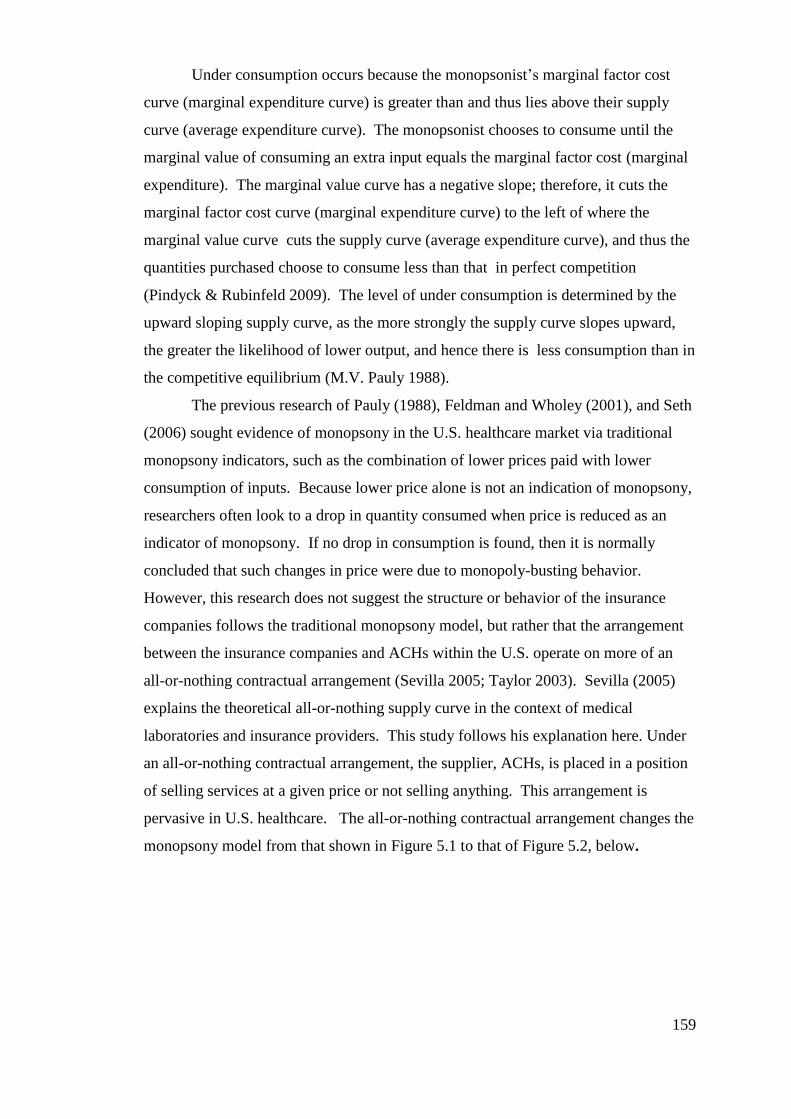
159
Under consumption occurs because the monopsonist’s marginal factor cost
curve (marginal expenditure curve) is greater than and thus lies above their supply
curve (average expenditure curve). The monopsonist chooses to consume until the
marginal value of consuming an extra input equals the marginal factor cost (marginal
expenditure). The marginal value curve has a negative slope; therefore, it cuts the
marginal factor cost curve (marginal expenditure curve) to the left of where the
marginal value curve cuts the supply curve (average expenditure curve), and thus the
quantities purchased choose to consume less than that in perfect competition
(Pindyck & Rubinfeld 2009). The level of under consumption is determined by the
upward sloping supply curve, as the more strongly the supply curve slopes upward,
the greater the likelihood of lower output, and hence there is less consumption than in
the competitive equilibrium (M.V. Pauly 1988).
The previous research of Pauly (1988), Feldman and Wholey (2001), and Seth
(2006) sought evidence of monopsony in the U.S. healthcare market via traditional
monopsony indicators, such as the combination of lower prices paid with lower
consumption of inputs. Because lower price alone is not an indication of monopsony,
researchers often look to a drop in quantity consumed when price is reduced as an
indicator of monopsony. If no drop in consumption is found, then it is normally
concluded that such changes in price were due to monopoly-busting behavior.
However, this research does not suggest the structure or behavior of the insurance
companies follows the traditional monopsony model, but rather that the arrangement
between the insurance companies and ACHs within the U.S. operate on more of an
all-or-nothing contractual arrangement (Sevilla 2005; Taylor 2003). Sevilla (2005)
explains the theoretical all-or-nothing supply curve in the context of medical
laboratories and insurance providers. This study follows his explanation here. Under
an all-or-nothing contractual arrangement, the supplier, ACHs, is placed in a position
of selling services at a given price or not selling anything. This arrangement is
pervasive in U.S. healthcare. The all-or-nothing contractual arrangement changes the
monopsony model from that shown in Figure 5.1 to that of Figure 5.2, below.
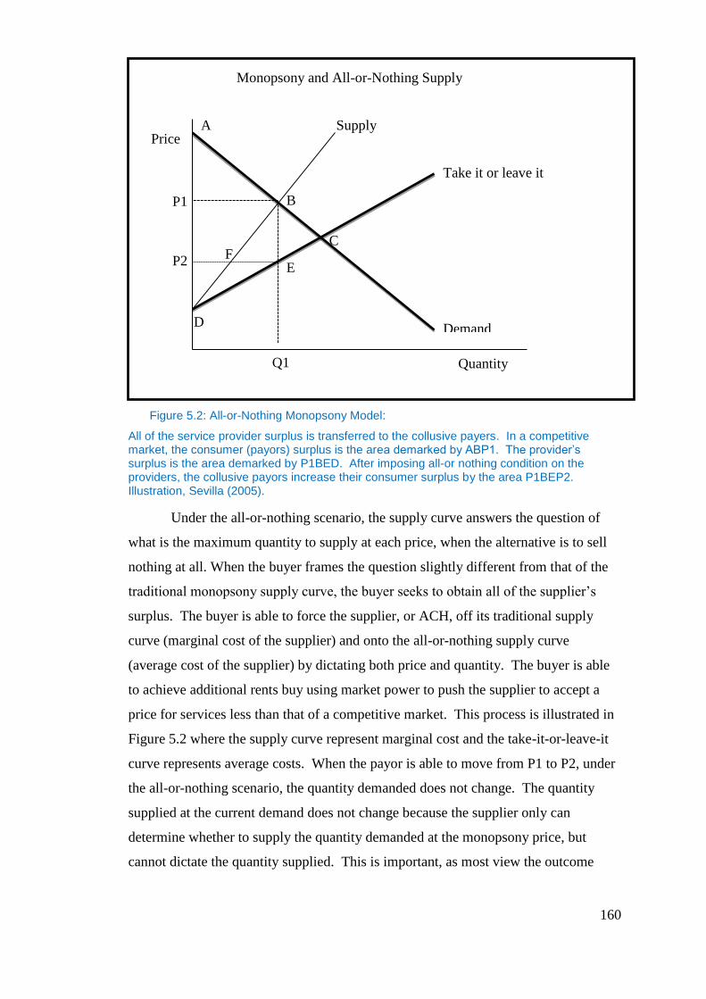
160
Figure 5.2: All-or-Nothing Monopsony Model:
All of the service provider surplus is transferred to the collusive payers. In a competitive market, the consumer (payors) surplus is the area demarked by ABP1. The provider’s surplus is the area demarked by P1BED. After imposing all-or nothing condition on the providers, the collusive payors increase their consumer surplus by the area P1BEP2. Illustration, Sevilla (2005).
Under the all-or-nothing scenario, the supply curve answers the question of
what is the maximum quantity to supply at each price, when the alternative is to sell
nothing at all. When the buyer frames the question slightly different from that of the
traditional monopsony supply curve, the buyer seeks to obtain all of the supplier’s
surplus. The buyer is able to force the supplier, or ACH, off its traditional supply
curve (marginal cost of the supplier) and onto the all-or-nothing supply curve
(average cost of the supplier) by dictating both price and quantity. The buyer is able
to achieve additional rents buy using market power to push the supplier to accept a
price for services less than that of a competitive market. This process is illustrated in
Figure 5.2 where the supply curve represent marginal cost and the take-it-or-leave-it
curve represents average costs. When the payor is able to move from P1 to P2, under
the all-or-nothing scenario, the quantity demanded does not change. The quantity
supplied at the current demand does not change because the supplier only can
determine whether to supply the quantity demanded at the monopsony price, but
cannot dictate the quantity supplied. This is important, as most view the outcome
Price
Quantity
Supply
Demand
Take it or leave it
B
A
C
D
E F
P2
P1
Q1
Monopsony and All-or-Nothing Supply

161
under an all-or-nothing contract as an efficient outcome because quantity supplied
does not change with the price, taking no consideration for supplier harm. Its
relevance will be revisited and evidenced later in this thesis. The additional rents
accumulated by the buyer/payor can be seen in the area of P1, B, E, and P2. Because
the quantity demanded did not change, there is no efficiency loss. The only loss is
that of the rents that are lost by the supplier (or ACH). Those rents or excess supplier
surplus then are recouped by the payor.
The difference between the traditional model of monopsony and monopsony
under the all-or-nothing supply curve is that traditional monopsony leads to a social
welfare loss. Under all-or-nothing monopsony, the monopsonist may be able to
acquire excess rents from the seller or input provider while maintaining an efficient
allocation of resources or inputs; however, the income allocation received by the
seller is less than in a competitive market, and is close to or at their average cost.
Suppliers, the ACHs that supply under an all-or-nothing scenario, may have supplier
profits pushed to zero, and in doing so, increase bankruptcy risk.
Firms placed onto the all-or-nothing supply curve find themselves with
restricted margins, and therefore restricted free cash flows. These distortions may
affect capital structure decisions within the U.S. healthcare market, and are the
concern of this research. Monopsony is possibly a distortion; therefore,
comprehension of its presence and effects upon capital structure are salient.
In the U.S., monopsony can explain the behavior of the ACHs regarding
capital structure and the amount of free cash flows that exist within the ACH market.
This research will examine the all-or-nothing contractual arrangement. This new
aspect will give a much greater insight into ACHs’ behavior in regards to capital
structure. The understanding of market behavior in the presence of monopsony, and in
particular collusive monopsony and its effect upon firms, capital structure, and
limitations placed upon their financial decisions is pertinent to financial research, as it
ultimately may be detrimental to firms, restricting their performance or increasing
their risk of bankruptcy.

162
5.1.2 Conditions for Monopsony
The research conducted in this thesis differentiates the ACH market from that
of a traditional monopsony to that of a collusive monopsony. In this case, collusive
monopsony describes the relationship between both government and commercial
payers to provide a restricted reimbursement scheme to ACHs within the U.S. The
existence of this particular relationship is allowed to continue because the U.S.
Government consumes more than 65% of patient days from ACHs annually
(determined using MCR data in longitudinal study of Chapter 4). The federal
government is under pressure to cover as many citizens as possible for the lowest
cost.
This creates pressure to provide healthcare at a below-market price, which is
compounded by the ratchet effect that occurs each year as the CMS recognizes the
ability of the industry to cope with lower and lower prices. Each year, the CMS
continues to lower prices until their actions are stopped politically, or ACHs’ attrition
from the program threatens its viability, thus ensuring the lowest price possible
without firm failure. The government is a low-cost payer for services in this market.
The CMS regularly releases information to the public regarding its policies and
payment practices, and these payment practices are inclusive of reimbursement
schedules in the form of a fee schedule by DRG. It consists of the diagnosis of the
patient, and results in a placement in a categorization. The price determined for each
categorization includes all cost and is capped in time by a length of stay measure.
Therefore, regardless of the length of stay, ACHs are paid only for the DRG. This
sometimes can be altered by the severity of the patient.
This public release of information allows other commercial payers within the
market to utilize this information to guide their own policies, procedures, and
reimbursement schedules. Commercial payers within the market then utilize this
knowledge to ratchet down ACHs’ reimbursements, thereby allowing the payor to
gain additional economic rents that otherwise would have remained with the ACH in
a more competitive/capitalistic market. While there is no intention on the part of the
commercial payers to collude with the CMS, it is their action of seeking additional
economic rents and the use of the fee schedules that present the environment for
collusive monopsony. The use of the CMS fee schedule by commercial payers
essentially creates tacit price fixing within the market, thereby reducing the

163
competitive nature of the market and increasing the inefficiencies within the market,
as evidenced in the laboratory services market discussed by Sevilla (2005). These
inefficiencies are the costs of the monopsony condition.
5.1.3 Antitrust
One might assume that monopsony would not be possible within the U.S., and
that the Sherman Antitrust Act would prohibit such an anti-competitive structure as
monopsony. However, previous research has suggested that U.S. courts do not
interpret issues of monopsony as inefficient or destructive under a standard of
consumer harm. This is important, as current conditions within U.S. healthcare would
be different if courts viewed monopsony in a negative light.
Hammer and Sage (2004) cited the existence of buyer-side market power and
the view of the consumer good provided by the use of buyer-side market power and
its ability to reign in healthcare costs, attributing it to the year 1984 and the ruling by
Judge Stephen Breyer in the First Circuit Court of Appeals in the case of Kartell v.
BlueShield of Massachusetts. The case involved balance billing by physicians.
Balance billing is when physicians accept payment by the insurer for services
rendered, yet seek compensation from patients for any outstanding balance left unpaid
by the insurance company. Blue Shield of Massachusetts, an insurance company,
contractually had prohibited physicians from balance billing. A group of physicians
had sued Blue Shield, claiming Blue Shield was the largest insurer in the state and had
used its market power to conduct unfair business practices primarily related to the
restriction upon physicians to balance bill patients, and therefore was in violation of
state and federal antitrust laws.
The judge ruled that Blue Shield had contractually prohibited balance billing
and therefore did not violate the antitrust laws, even though the defendant in the case
was the largest insurer in the state at that time. In this case, Judge Breyer did not look
at Blue Shield as a separate entity within the market, but rather as a buying group;
therefore, any discounts forced on physicians would flow through to the insured, and
consequently, premiums would be discounted. Judge Breyer, “focused on the
centrality of the insurer-insured agency relationship thereby framing the dispute in a
manner where he could conclude that Blue Shield’s conduct did not create antitrust
liability, even assuming Blue Shield possessed and exercised significant market
164
power” (Hammer & Sage 2004, p. 955). The judge did not regard this market as two
separate markets, one for purchasing healthcare services and one for health insurance,
but combined those markets into one single market in which insurers were just buying
agents for the insured, and therefore physicians were obligated to accept the
discounted rate in return for the purchaser’s quantity (Hammer & Sage 2004).
This notion that the insurer is nothing but a buying agent disregards the fact
that insurance is a product itself and has its own markets with its own profit motives
that are derived from inputs of purchased health services. Insurance is a financing
mechanism for purchasing health services. The consideration of insurance, as two
markets, is a key concept carried forward in this research and is a primary
consideration of the profit maximization under monopsony. In his decision, Judge
Breyer also failed to verify that the lower input prices of purchased health services
actually lowered premiums to the insured of Blue Shield. The monopsony issue was
completely ignored, as Breyer failed to realize that a monopsonist maximizes
economic rents (Hammer & Sage 2004).
The judge also was concerned that antitrust law might be used to try to
regulate the healthcare industry, and left the responsibility up to regulatory agencies
within Massachusetts to take on that burden. This decision failed to ensure proper
competition within the market itself, as it did not take into account that discounts are
not passed on necessarily from the insurance to those being insured. Hammer and
Sage (2004) hold that although the Breyer decision was a relatively contextualized
ruling, further court cases involving healthcare antitrust have utilized this case as the
foundation to suggest that insurers stand in and act on behalf of those they insure.
Distortions of the idea presented by Judge Breyer have been used to defend
exclusionary activities of buyers, “health insurers,” which would violate Article 2 of
the Sherman Act. In Ocean State Physicians Health Plan v. Blue Cross, the court
upheld that having a policy that insisted on a supplier’s lowest price was not in
violation of the Sherman Act, as long as it was not predatory or below the supplier’s
incremental cost, and in fact would be promoting competition. The Kartell case has
been used to substantiate decisions in favor of insurers; however, the Kartell case and
others similar to it provide an inadequate basis from which to evaluate medical
monopsony power, because they fail to see the insurance market as two separate
markets (insurance and health services), and assume that savings or excess rents
165
generated from insurers predatory practices are passed on to the consumer (Hammer
& Sage 2004).
While monopsony continues to be addressed in non-healthcare arenas in the
U.S., as per the Supreme Court’s decision in Wyerhaeuser Co. v. Ross-Simmons
Hardwood Lumber Co., 2007 (Rosenfelt 2008), it is unlikely to be addressed the same
way in healthcare, as healthcare is seen to be unique by many. As James Robinson
(2001, p. 1045) expressed,
“…the salient characteristics of health care, including professionalism,
licensure, nonprofit organization, third-party payment, and heavy government
regulation, can be found in other sectors, albeit not bundled in quite the same
distinct and dysfunctional manner. The uniqueness doctrine hence proves too
much. More importantly, the principle serves as a two-way barrier to entry
between the health and non-health sectors. In one direction, it discourages
mainstream economists from importing the principles of industrial
organization, game theory, and transactions costs to health care issues by
raising a wall of acronyms and institutional trivia that impedes dialogue. In the
other direction it fosters complacency among the virtuosi of health policy
analysis, allowing us to achieve fame and fortune in our small pond without
fear of competition from denizens of the scholarly shark tank.”
If mainstream economists are unwilling to venture into a new area fraught
with “walls of acronyms and institutional trivia that impedes dialogue,” then certainly,
very little progress can be made to help courts understand the inefficiencies within
healthcare and how consumer harm is established by allocative inefficiencies
(Robinson 2001, p.1045). Robinson (2001) condemned the views expressed by K.J.
Arrow (1963), which via asymmetric and imperfect information, justified the rationale
for the existence within healthcare of, “every inefficiency, idiosyncrasy, and interest
serving institution in the healthcare industry,” basically stating that the rationale for
non-traditional contracting and organizations and their market responses were, in
effect, an “efficiency-enhancing” response to the limitations of information (Robinson
2001 p.1046). Robinson further explained that Arrow used such interpretations of
distortions within the healthcare market to justify antitrust exemptions reducing costs,
and that consumers are incapable of comparing insurance plans and must yield this
function to politicians (Robinson 2001). Therefore, it is understood how judicial
166
decisions regarding monopsony could become distorted with regard to market
inefficiency when underlying literature supports such views, especially when one
considers that in addition to the literature, the courts use an out-of-date model to
measure consumer harm. Such is the case with the ancillary restraints model.
Alexander (2007) addressed the use of Blair and Harrison’s ancillary restraints
doctrine and its use by courts in interpreting cases of monopsony. The ancillary
restraints doctrine is used to judge cases of monopoly, The ancillary restraints
doctrine defines that agreements among competitors are illegal unless the
defendant/competitors can show that the agreement has pro-competitive benefits and
that the overall effect is good for the consumer (Alexander 2007). Alexander (2007)
pointed out that the overall quest of the model is to correct consumer harm, but
appropriately, it gives evidence that within a situation of monopsony, it is not the
consumer that is harmed, rather the supplier. Because courts interpreting monopsony
cases have validated the ancillary restraints model explicitly as a determinate method,
this has left economists and attorneys with a void left from this model’s inadequacy,
as it mostly addresses consumer harm.
The ancillary restraints model views monopsony similarly to monopoly in that
the case is judged on a few parameters. According to Alexander (2007), the defendant
must address three issues when addressing the ancillary restraints doctrine: 1) The
agreement must be shown to increase competition; 2) Price fixing is a necessary evil
in order to bring about the benefits of increasing the nature of competition; and 3) The
agreement is only as restrictive as necessary to bring about these benefits. Alexander
addressed the shortcomings of the ancillary restraints theory of monopsony within the
courts by offering additional insight into the Sherman Antitrust Act and its intended
beneficiaries. She identified the shortcomings of the ancillary restraint model and
analyzed the arguments used to fill in where the ancillary approach fails.
The ancillary restraints model does not concern itself with harm to the
supplier, only to the consumer. However, supplier harm is an inefficiency of the
market that ultimately may harm consumers, just not directly. Zerbe (2005)
recognized the harm created by such inefficiencies. Zerbe had suggested that
agreements should be analyzed for inefficiency of markets, stating that ultimately, all
consumers are harmed by inefficiency. Zerbe felt that any time the price for a product
deviated from marginal costs, resources were wasted. He suggested that resources
167
have an opportunity cost. The limitation of resources, due to monopsonistic
inefficiency, has repercussive effects for those resources other uses and/or markets,
and the use of these resources in alternative markets would be beneficial to consumers
in those markets. Monopsony prevented the use of such resources in other markets;
therefore, the consumers were harmed. Additionally, he suggested the idea that the
identification of consumer price changes to consumers for a limited set of markets is
incorrect, and suggested that consumer and producer surpluses are the income
equivalent measures of welfare. Zerbe saw both consumer and producer surplus as a
measure of reduction in satisfaction. According to Zerbe, the use of economic
efficiency as the general standard is a reasonable assumption; consumers will lose
from inefficiency wherever it is found. The presumption should be that the market
distortion introduced by the monopsonization will cause consumer harm, both in the
output market and in all related markets taken together (Zerbe 2005). This is an
important and salient point to this research as the inefficiencies of monopsony are
suggested to have lasting effects on ACH margins and free cash flows, therefore
possibly limiting their access to debt markets, which affects ACH decisions of capital
structure.
According to Alexander (2007), these arguments fall into two separate
categories, those that claim monopsony harms end consumers, and those that claim
the Sherman Act is intended to protect society and others in the economy and not just
end consumers. She pointed out that the arguments made by Zerbe (2005) are
incorrect and inefficient, stating that it would be more efficient to ban buying cartels
than actually to analyze the effects of the agreement at hand. The other problem with
Zerbe’s argument, according to Alexander (2007), is his promotion that, “effects in
other markets to show harm to consumers,” was rejected by the Supreme Court as a
methodology for judging consumer harm, not to mention that it is very similar to the
current consumer welfare standard in use today Alexander (2007, p.1629).
Others argue that consumer harm should not be the relevant standard against
which monopsony cases are held. According to Alexander (2007), individuals within
this ideology fall into two categories. They are: 1) those individuals who argue that
cases should be measured by aggregate efficiency for antitrust purposes; and 2) those
who argue that the Sherman Act protects others within the economy equally well as
consumers. Those who believe that aggregate efficiency should be the criteria by
168
which monopsony cases should be decided are wrong, because this is contrary to
legislative intent, according to Alexander. She held that while it may be good
economic policy for antitrust laws to guard against allocative inefficiency, the
Sherman Act was created prior to economists’ understanding of allocative efficiency.
Therefore, the legislature’s intent could not have incorporated the use of allocative
efficiency as the basis for antitrust jurisprudence. Alexander pointed out that those
who believe that the Sherman Act protects all others should consider the legislative
history of the Sherman Act. The act clearly demonstrates a concern for consumer
welfare.
In her paper, Alexander (2007) concluded that under the Sherman Act, it is
important that aggregate efficiency and consumer prices are utilized in evaluating
contentious agreements, but that these conditions are restricted when courts consider
the legality of the agreement itself. It is the consideration of competition over
efficiency or consumer prices that fills the gap of the ancillary restraint model. She
considers it the job of Congress, not the courts, to determine if the Sherman Act
should reflect sound economic policy. The previous courts decisions as well as
academic literature are helpful in understanding how monopsony could be present in
the healthcare market in the U.S. despite antitrust legislation. This environment
described in the literature around healthcare antitrust is one in which monopsony
could easily be present and readily survive as a market presence. Therefore, it is
important to understand monopsony from an academic research perspective.
5.2 Monopsony in Literature
5.2.1 Literature
Due to the structure of the previous monopsony research, a relevant analysis
of monopsony in literature will be considered within two categories in this
subchapter: non-healthcare related and healthcare related. The first category, non-
healthcare related, will be addressed in Section 5.2.1.1, followed by healthcare related
in Section 5.2.1.2. Non-healthcare-related research helps establish this study within a
larger research context, while the healthcare monopsony research helps to refine the
positioning of this research in relation to more specific monopsony discussions in a
healthcare context.

169
5.2.1.1 Non-Healthcare Monopsony Research
Non-healthcare monopsony research previously has focused on markets that truly
exhibit monopsony conditions, and considers markets such as labor markets, poultry,
or meat-processing markets for hogs and cattle, in addition to markets for public
goods. In many nations, healthcare is considered a public good. In the U.S.,
healthcare can be viewed as a public good provided by an agency relationship
between ACHs and the government and private insurers. Bish and O’Donoghue
(1970) used a simple two-person model in a world in which there is a public good and
at least one private good to examine equilibrium outputs of public goods, which result
from consumer cooperation under conditions of both constant and increasing costs.
They argued that if a market for public goods is under an increasing cost environment
with monopsonistic demand articulation, the under consumption of the public good
was likely. They suggest that monopsonistic environments are to be created under
these conditions, as the articulation of demand is likely to come from individuals
represented by a monopsonistic organization (Bish & O’Donoghue 1970). They
suggested that this was true, as bargaining costs are high, and consumers of public
goods are numerous. This encourages individuals to be free riders; therefore, they
would wait for others to provide the public good. Bish and O’Donoghue (1970)
suggested that under these conditions, the government and/or private demand
articulating groups would emerge and incentivize individuals to join their groups.
These groups would then act as monopsonistic buying groups. This is similar to the
conditional environment set forth in this research between CMS and private payors,
because they behave as a collusive monopsony to purchase healthcare services on
behalf of individuals. In this case, the present research examines the market of a
public good, healthcare. Healthcare within the U.S. is under increasing cost
constraints. If monopsonistic demand articulation is present underconsumption of the
good is likely. While Bish and O’Donoghue (1970) remain valid, they express
monopsony under a traditional context, which does not accurately describe the
outcome the consumption equation. This divergence of traditional monopsony and
monopsony under the all or nothing contract allow for outcomes more favorable to the
consumer and the payor. This provides a basis for the models discussed further in
chapter 6.

170
Hirofumi Shibata (1973) suggested that Bish and O’Donoghue (1970) may
have been accurate, but refuted that the condition of increasing cost of the public good
is a necessary market parameter for monopsony to exist. Constant costs as well as
increasing costs could also be an environment in which monopsony might exist.
Shibata (1973, p. 223) pointed out that under the increasing cost of a public good, the
presence of income redistribution affects, “a non-cooperative party solution, one
involving over-consumption rather than under-consumption.”
This view is counter to monopsony theory, in which the presence of
monopsony leads to underconsumption due to the inefficient allocation of resources
(inputs), as was displayed in Figure 5.1. While Bish and O’Donoghue (1970) assumed
that producers of public goods are price takers rather than price makers, Shibata
(1973) holds that both a monopsony and monopoly could exist when one party is a
price taker and the other a price maker. Taking issue with Bish and O’Donoghue’s
(1970) premise that producers of public goods could not be consumers of public
goods, Shibata pointed out that once a public good is produced, all within a given
economy are free to consume that good. Shibata held that both monopsony and
monopoly could exist in markets for public goods where neither party is the price
taker. He suggested the assumptions that the consumer can cooperate while producers
cannot, and that the producer can cooperate while consumers cannot, are unrealistic,
unless asymmetric institutional or behavioral assumptions are included (Shibata,
1973). The presence of asymmetry of information is an important concept in
healthcare in the U.S. and the research presented here. There is asymmetry of
information in the consumption of healthcare as most patients are ignorant of the
services they receive. This transactional model is further complicated because the
purchaser or payor has little information of services delivered as well (Mirmirani and
Spivack, 1993; McLean 1989; Schneider and Mathios 2006).
If monopoly or monopsony does exist in the market for public goods, then the
environment is conducive to over- or under consumption, barring strategic behavior;
that is to say that a Pareto-optimum outcome could not exist. Shibata (1973)
concluded that in the case of public goods and increasing cost versus constant
cost/monopsony, under consumption is not the major concern, but rather what is of
concern is the possible existence of a monopoly and overconsumption due to income
redistribution or the situation of a bilateral monopoly under which both over and
171
under consumption equally are possible. However, under increasing cost conditions,
overconsumption becomes the larger problem. Shibata held that the effect of
redistribution of income is significant under majority rule, as the proportion of the
population that suffers from the redistribution of income often has no effective way of
preventing the production of the public good by the other party or being financed by
the taxes imposed upon them.
Overconsumption is an important characteristic of U.S. healthcare as it not
only suggests the existence of a moral hazard created by the presence of insurance,
but in an increasing cost setting, overconsumption is could be due to an income
redistribution mechanism within the Medicare/Medicaid framework. This also
describes the legal framework under which healthcare is supplied in the U.S., in
which ACHs are required to deliver healthcare under unfunded mandates and lower
reimbursements than Pareto-optimum conditions. These constructs described by Bish
and O’Donoghue (1970) and Shibata (1973) help to provide a basis upon which the
theoretical model of this research is based. Newhouse (1981) and Glied (2003)
further support this idea of overconsumption due to moral hazard of insurance in U.S.
healthcare. In addition to markets for public goods, one primary area of focus for
monopsony research has been labor markets.
Labor long has been an environment for the study of monopsony, and can be
correlated and helpful in determining the consequences of its existence in healthcare.
Usually, firms that are studied are isolated geographically, and therefore have market
buyer power in the surrounding markets of labor. Michael Bradfield (1990) examined
the long-run consequences of monopsony in this context. Bradfield used the
traditional monopsony model and the Cobb-Douglas production function to lay
framework for his argument. He assumed monopsony power only in the input labor
market, while the firm operates in a competitive market in the output market. This
allowed Bradfield to show that the long-run equilibrium for wages and quantity of
labor are lower than in a competitive labor market, even under the presence of a union
representing the input labor.
Backwards integration in the healthcare market has been thought to exist
because payors may try to internalize the inefficiencies of the input market. An
example of this is where HMOs directly control the production of healthcare, and
therefore better control cost, thereby allowing them to become more competitive in
172
the upstream markets of health insurance, which is typical behavior of a monopsonist.
In U.S. healthcare, there have been several efforts by HMOs to integrate backwards
into supplying healthcare directly. Likewise, Azzam (1996) showed that there may be
incentives for backwards integration in order to internalize inefficiencies of the input
utilization of monopsony itself. Azzam examined the U.S. beef slaughter industry,
applying Perry’s (1978) theory of backward partial integration in order to derive the
equilibrium condition for a profit-maximizing vertically integrated monopsonist firm
that competes with a finished product in the final consumer market.
Partial backwards integration is a measurement of backwards integration that
is independent of the production decision made by a monopsonist. The methodology
allows for the examination of the impact of backwards integration on the choices of
input production. The partial integration allows for the assessment at each subsequent
degree of integration. This allows for consideration of the welfare implication and
incentives for further backward integration by the monopsonist.
Under Azzam’s (1996) study, the monopsonist only may integrate partially, as
post-integration profits also include monopsony inefficiencies plus the economic rents
derived from the target. Given that the monopsonist will have a purchase price for the
target, the monopsonists are likely only to partially integrate when considering the
cost of acquisition, internal cost of production, and the additional economic rent.
Azzam concluded that there is support for the monopsonist’s backwards integration
when taking inefficiency into consideration in the model. He suggested caution for
his research, as there may be other considerations taking place in backward
integration that are not considered within his research examples, such as transactional
economies and market imperfections.
Therefore, while a monopsonist may integrate backwards to internalize input
market inefficiencies, it does not have to be full integration to realize some additional
economic rents. Likewise, in the U.S. healthcare market, HMOs and MCOs have
tried to internalize some of the production efficiencies into their organizations in order
to be more competitive in the market for health insurance. This is typical
monopsonistic behavior; however, traditional monopsony does not accurately
describe the contractual nature, which is prevalent. It is monopsony under the all-or-
nothing contract that should be considered.
173
Taylor (2003) examined monopsony under the conditions of an all-or-nothing
contractual situation. Taylor argued that a monopsonist with market power could
leave little options for suppliers of inputs. Suppliers are offered all-or-nothing
contracts in which the supplier can accept and supply goods at the defined
monopsonist rate, or supply nothing. Due to the quantity buyers represent, the
supplier has little option because of the exploitation of the producer’s surplus. Under
this scenario, the input supplier is moved off its marginal cost supply curve and onto
the average cost curve. Taylor used a traditional monopsony model augmented to
adjust for the all-or-nothing condition, suggesting that the monopsonist exploitation of
the all-or-nothing contract leads to an efficient allocation of input resources. In other
words, under this all-or-nothing contract, the market would have efficient allocation
of inputs to the market; thus, there would be no decrease in quantity demanded.
However, the monopsonist would gain the surplus economic rents derived from the
supplier, and therefore, input prices would be allocated inefficiently. Thus, the
monopsonist would accrue all profits normally attributed to competitive input
suppliers.
This is supported when one considers that the standard supply curve provides
the quantity that suppliers will provide at every possible price. This combination of
supplied quantity and price for various prices form the usual supply curve. The
seller’s choice is how much to supply at a particular price. According to Blair and
Harrison (1993), the all-or-nothing supply curve is different. It reveals the maximum
quantity suppliers will make available at each price when the alternative is to sell
nothing at all. The all-or-nothing supply curve lies below the standard supply curve.
This enables the monopsonist to exploit the seller by pushing the seller off its
traditional supply curves and onto the all-or nothing curve (Blair and Harrison, 1993).
Taylor (2003) concluded that monopsonist firms that take advantage of the all-
or-nothing supply curve in a competitive input industry will have a socially efficient
allocation of resources. However, he pointed out that the distribution of income will
not be equitable in comparison to competitive markets, as the monopsonist will have
appropriated all the excess rents from the input suppliers. He commented that while
there may be no need for antitrust legislation to mediate for efficient allocation of
resources, there should be some concern and interjection to deal with the,
174
“distributional consequences of exertion of all-or nothing-buyer power” (Taylor 2003,
p. 14).
Taylor’s (2003) work provided support for antitrust positions that monopsony
can lead to the competitive market allocation of resources leading to increased
consumer welfare. Therefore, there is no need for intervention within a
monopsonistic buyer market with these characteristics. This is important to the
research in this chapter, as this helps us gain some understanding as to why one might
not interfere within markets with monopsonists utilizing the all-or-nothing contractual
arrangement, especially when one considers the antitrust environment discussed
previously. This is also important because this contractual arrangement is
predominantly the contractual arrangement that occurs within the ACH market
between ACHs and insurers, both government and commercial.
de Fontenay and Gans (2004; hereafter DG), carried the research of vertical
integration further, investigating whether vertical integration by a monopsonist causes
consumer harm. They suggested that under a normal economic environment, the
monopsonist and the consumer interests are not aligned in regard to vertical
integration. They modeled one-on-one bargaining between a monopsonist and
independent suppliers when the set of suppliers cannot be expanded easily ex-post.
They showed that a non-vertically integrated monopolist is susceptible to holdup.
They suggested that without integration, a monopsonist has an incentive to encourage
more upstream entrants than normally would occur in a neoclassical monopoly.
Having more suppliers alleviates the holdup problem. This increases industry output
and lowers the industry marginal costs in order to increase the monopsonist’s
bargaining position. Vertical integration mitigates the hold-up problem faced by the
monopsonist, and vertical integration allows the monopsonist to generate and
appropriate an increased level of industry profits at the expense of consumers. DG
expressed that most concern for consumer harm is achieved when the monopsonist
forces the exit/foreclosure of suppliers from the input market. This is a salient point
as courts have failed to see this concern, which allows monopsony to exist and allows
monopsonistic behavior to affect ACHs, which consequently have effect on their
capital structures decisions.
Inoue and Vukina (2006) further analyzed the presence of monopsony power
in agency contracts within the livestock industry. They observed the impact of the
175
livestock integrator on the market for contract growers. The model examined the
relationships between the observable consequences and unobservable grower
characteristics. This is accomplished by imposing first-order conditions for the
principals’ profit maximization. Their research states three reasons why the grower
market is not competitive and might have monopsonistic characteristics: 1)
Geographical areas show differentiation in the levels of competition for growers; 2)
Market power may be derived from contracts with integrators and the necessary
investment to produce inputs; and 3) Production contracts in animal agriculture
contain issues of moral hazard. In this last case, the monopsonistic behavior arises
from the integrator facing an upward sloping supply curve as a result of having to pay
the grower more for greater effort. The integrator/monopsonist must use more
resources to ensure compliance, and therefore hires fewer workers, in other words,
below competitive levels.
Inoue and Vukina’s (2006) model used three performance indexes: live grain,
mortality, and feed conversion. They used these three indexes in a first-order
condition to maximize the integrators profits. Estimating with the generalized method
of moments (GMM), using data on the individual grower contracts and one primary
integrator, they found that no monopsony is present in this market. They attributed
this to the fact that integrators may not have to pay higher fees for higher output of
production, stating that they do not believe the sample is representative of the market
as a whole. This outcome is important as it suggests that not all environments, which
are ripe for a monopsonist, actually create monopsony. The research of Inoue and
Vukina (2006) provides a contra argument for the research presented within this thesis
and is included to show that it is necessary to conduct research akin to this thesis, as
the outcome is not a forgone conclusion even though there is clear evidence to suggest
that certain market constructs should be present.
5.2.1.2 Healthcare Monopsony Research
Monopsony in healthcare is discussed widely throughout literature, although
initially it was discussed as an allocative efficiency issue. The healthcare industry is
known to have distortions that affect the market: moral hazard, agency, and the
allocative efficiency issues (monopsony/monopoly), amongst others. Researchers
long have tried to further understand the healthcare market within the U.S.
176
Philip Hersch (1984) examined competition and market efficiencies within
non-profit hospitals. Hersch created a theoretical model that assumes that hospitals
compete in the market for physicians based upon hospital prices and resource
allocation. Hersch argued that an increase in market concentration results in raising
hospital costs when adjusted for quality, ultimately reducing hospital admissions and
the quality of care per admission. Theory would predict that hospital prices, adjusted
for quality, should increase with market concentration. Hersch’s study lacked any
measure for quality, and therefore used a proxy. The proxy said that higher prices
would be shown in reduced admissions and the length of stay in the hospital.
Hersch (1984) used a sample of 260 Standard Metropolitan Statistical Areas
(SMSAs) and six potential 1972 SMSAs to create a regression of hospital stays and
quality measures. Hersch utilized total expenditure per admission as a proxy for
hospital care. Hersch concluded that despite the fact that the hospitals within the
study were nonprofit, they exhibited profit-maximizing behavior. Hersch explained
that the implications of the market structure of healthcare are consistent with
previous empirical results that market competition plays a central role in overall
market performance. In Hersch’s case, this led to higher admissions and greater
levels of hospital care per patient. His results suggested that efforts to control costs
via competitive forces have been counterproductive, because competition has raised
the cost of healthcare by increasing the level of care provided per admission. The
increases in cost more likely are the result of a misallocation of resources as a result
of extensive hospital insurance. The extensive hospital insurance, because of the
moral hazard, decreases the allocative efficiency of competition (Hersch, 1984).
Hersch (1984) recognized the implications of the moral hazard and its possible
ability to distort markets for healthcare. Competition under this moral hazard is
skewed, and hospitals compete for patients and physicians utilizing mechanisms other
than prices. Quality certainly is one of these competing variables, as is the resources
for both patient and physician. Along with Hersch’s empirical results, these
distortions help explain the excessive capitalization and thus overinvestment found in
the ACHs and mentioned in this research. Hersch (1984) findings are important as
they suggest that first, non-for-profit hospitals exhibit profit maximizing behavior.
Second, that moral hazard of insurance is prevalent and causes distortions within the
market, which provides perverse incentives to providers and increases the costs of
177
providing services. All of these are issues payors seek to control and as a
consequence reduce the amount of inefficiency inherent in the supplier market.
Mirmirani and Spivack (1993) examined the causes of distortions found within
the healthcare market and used these distortions to explain any deviation from Pareto
efficiency. They cite five reasons for the deviation from Pareto efficiency: 1) lack of
competition; 2) insufficient/asymmetric information; 3) inadequate access to health
care services; 4) presence of externalities; and 5) market disequilibrium (Mirmirani &
Spivack 1993). They pointed out that these are all reasons for the failure of the
healthcare market within the United States.
Considering the lack of competition, Mirmirani and Spivack (1993) suggested
that special interest groups within healthcare determine the supply of healthcare,
conspiring to keep incomes up by restricting supply. They suggested that two major
groups, the AMA representing doctors, and the AHA representing hospitals hold the
majority of control. These two organizations have turned over, changed, or blocked
the majority of legislative policy decisions by the U.S. Government to benefit
themselves. The AMA has reduced supply by lobbying against allowing foreign
medical graduates from entering the U.S. to practice, and at the same time, reduced
the amount of students accepted for medical school at U.S. institutions.
Studying hospital markets, Mirmirani and Spivack (1993) pointed not only to
the special interests influencing policy, but also to the failure of HMOs to increase
competition. This is because the HMOs need to compete against larger, better, and
more expensive technologies that cause their premiums to climb. This ultimately
resulted in HMOs’ inability to compete in the marketplace, and therefore they had less
impact on the overall competition level. As previously determined, providers of
healthcare compete on variables other than price. Healthcare consumers within the
U.S. value quality above price. This is driven primarily by the moral hazard created
by the heavy presence of health insurance within the market. In this case, health
insurance insulates the patient from the prices of healthcare. If individuals were to
pay for their own healthcare, then these variables of technology and quality would be
lessened as a determinant of market share, as individuals would strengthen the
importance of price in the equation for determining health consumption. Currently,
individuals with health insurance, whether from government or private insurance, are
not exposed to concerns of price in consumption of healthcare. Thus, the moral
178
hazard of insurance is present. Moral hazard effects are heightened by the lack of
information on the part of the patient consuming the healthcare services.
According to Mirmirani and Spivack (1993), insufficient information or
asymmetric information exists within healthcare. They noted that all information
regarding healthcare services is located within the servicing body, whether physician
or hospital. The lack of information on the patient’s behalf causes the patient to incur
higher costs in order to acquire healthcare services. Mirmirani and Spivack promoted
advertising as a method of reducing this asymmetry of information, by educating the
patient on the services offered and the benefits of such services. They argued for
advertising, which at the time of their research was illegal; however, advertising since
has been utilized by both physicians and hospitals, lowering the informational
disparity that was prevalent at the time of their research. This is not to say that
informational asymmetry has been removed completely from the provisioning of
healthcare, as it has not.
Mirmirani and Spivack (1993) promoted inadequate access to healthcare as a
reason for the inefficiency. They also outlined the impact that externalities can have
upon the healthcare market. Mirmirani and Spivack pointed out that disease
epidemics as well as medical malpractice lawsuits can have large impacts on the
operations of the healthcare market. Their example cited a case of Acquired Immune
Deficiency Syndrome that led to an increased level of insurance claims and treatment
expenditures in the 1980s, and they anticipated this epidemic would add additional
burdens to the health market. Further, medical malpractice lawsuits cost the sector
$2.6 billion by 1988 (Mirmirani & Spivack 1993). In both cases mentioned, they cite
the government as the intervener of choice.
Market disequilibrium is discussed by Mirmirani and Spivack (1993),
suggesting that a continuous disequilibrium exists due to excess demand causing
inflation within the market. They cited Mirmirani and Otts’ (1990) suggestion of
increasing the patients’ contribution of payment in order to reduce the overall
disequilibrium within the market. Mirmirani and Spivack (1993) concluded that in
order to countermand these market imperfections, the only solution is one in which
healthcare is provided for all via a government plan, as all citizens would have equal
access to healthcare. This would remove the inefficiencies within the market of
inadequate access to healthcare, which they saw as an underlying cause of the
179
inefficiency. According to their view, a capitalistic market is incapable of handling
healthcare, and only a socialist system of free healthcare with equal access resolves
such disequilibrium. Mirmirani and Spivack (1993), provide additional evidence for
the context and construct of monopsony within U.S. healthcare by payors, ultimately
suggesting that a single buyer solution organized by the government is the only
solution. In other words, the only methodology moving forwards is a monopsonist
within the market controlling the input market of health services.
Mark Pauly (1998) examined the disequilibrium within healthcare, suggesting
the theoretical possibility of monopsony behavior by managed care insurance
providers. He used microeconomic theory to investigate how managed care plans
acting as a monopsonist might behave, and the expected effects upon the consumer
and supplier welfare. His interests in monopsony were driven by concern that
antitrust courts misunderstand monopsony. He opined that the measurement of
consumer welfare that is used as a mechanism for the justification of the presence of
monopsony within the marketplace may need to be reexamined when interpreting
decisions in healthcare. He suggested this because monopsony does not necessarily
reduce the welfare of the end consumer. Therefore, the goal of antitrust law,
consumer protection, and the objective of economists of welfare maximization may
need to be revised in light of monopsony, because consumer harm and economic
inefficiency is not readily apparent.
Pauly’s (1998) second reason for concern was that it may be difficult to
recognize the inefficiencies of lower prices for healthcare as below the competitive
level, especially in light of the previous monopoly power held by providers, in other
words, a monopoly breakup. The lower prices may be interpreted as monopoly-
breaking activity. Pauly used the traditional definition of monopsony power with its
outcome of lower input prices and lower consumption of the input. Pauly (1998),
defines inputs as ACH services purchased by managed care providers.
Pauly (1998, p. 1444) further stated that the input market monopsony, “arises
when there is only one managed care play (buyer) in a local market, but there are
multiple competitive sellers of that service, and when the market-level supply curve
of those services is upward sloping.” Pauly noted that it is difficult to tell if
monopsony is taking place just from the presence of lower prices for inputs, or if it is
bilateral negotiations taking over from a monopoly on inputs by the seller. The
180
delineating variable is the quantity of inputs acquired by the buyer, as mentioned
previously. He modeled both a traditional single-buyer market monopsony as well as
a partial monopsony, which consists of a large dominant buyer with monopsony
power with additional fringe buyers without monopsony power in the marketplace. In
both cases, Pauly conceived that monopsony is possible in both markets; however,
monopsony in the partial monopsony market is not as clear. His partial monopsony
market in healthcare is similar to the argument in this research of collusion between
the U.S. Government and commercial insurers. The U.S. Government acts as the
dominant firm, and the commercial insurers act as fringe buyers. The research
conducted within this thesis seeks to potentially clarify the existence of monopsony
within the healthcare market, by finding empirical support for the theoretical work by
Pauly (1998).
The consideration of monopsony by MCO’s/HMOs was revisited by the
research of Feldman and Wholey (2001). Feldman and Wholey designed a two-stage
study to determine the market power of HMOs and whether monopsony power exists
under the traditional definition (monopsony implies lower input prices and lower
consumption of those inputs). Using time series data on all HMOs operating within
the U.S. from 1985 to 1997, they estimated regression equations to explain prices paid
by HMOs for ambulatory visits and inpatient hospital days in terms of the importance
of HMOs as a buyer of these services. Next, they regressed the utilization of
ambulatory and hospital services per enrollee of an HMO to determine HMO buyer
power. They found that increased HMO buying power does reflect monopsony
conditions, as input prices lowered, but utilization of the inputs increased. According
to their research, this can be attributed to the continued breakup of monopoly power
of hospitals. Thus, Feldman and Wholey concluded that HMO buying power
improved the efficiency of markets for hospital services.
This is notable, as the traditional model for monopsony does not describe the
healthcare market accurately, or the contracted relationships therein, because markets
for healthcare services often operate under an all-or-nothing contractual basis.
However, Feldman and Wholey (2001) made an incorrect assumption that the
traditional definition of monopsony will provide an accurate model for use in the case
of U.S. healthcare markets. They assumed that hospitals could provide partial
quantities to the HMOs, instead of HMOs and insurers using all-or-nothing

181
contractual arrangements with the providers of healthcare services. This incorrect
assumption erodes their interpretations of the results. In the case of an all-or-nothing
relationship, utilization or quantity demanded would increase while prices decrease,
as ACHs must either supply the quantities demanded at the offered price or supply
nothing. Their interpretation that the continued breakup of monopoly power results in
increased efficiency of the market is misleading. Feldman and Wholey’s approach is
similar to the research conducted within this thesis; however the monopsony model
discussed within this thesis perhaps more accurately depicts the relationship of the
payor and hospital. This provides a more complete answer to the monopsony question
and its effects upon decisions of the capital structure of ACHs in U.S. health care.
M.V. Pauly (2004) examined the concepts of quality in healthcare and
competition’s effects on quality in the marketplace. His paper mainly focused on
hypothetical cost quality tradeoffs in the presence of competition and the
ramifications of such. He defining quality as, “everything about some good or service
relevant to consumers (actual and perceived ) welfare that is not measured by
quantity” (Pauly 2004, p.114) , and argued that quality and price often trade off
eventually, and that competition will make consumers better off, but will not be able
to maximize quality. He also argued that the cost of such quality has an impact on a
firm’s financials, whether as leverage or liquidity. He maintained that due to
distortions within the market, such as the “medical arms race” previously noted in this
research, the distortions have an impact because it has been shown that firms that
cannot compete on price compete on quality, whether real or perceived (Robinson &
Luft(1985). However, he further noted that the average level of quality may be lower
than if the market consisted of a competitive environment resulting from the ceiling
on price precluding high quality at a higher price. What Pauly (2004) expressed in his
research is relevant, because it continues to suggest that ACHs, even under restriction,
still compete on quality because price is not a factor, and that the market is restricted
by asymmetric information and by artificial pricing. It is also important as it expands
the possible measurement for monopsony. This is salient as it provides a contextual
reference for how monopsony is measured within research.
Allocative efficiency of the healthcare market was also examined by D.L.
Sevilla (2005). He proposed that a collusive monopsony exists in U.S. laboratory
services between government and commercial insurers who collude to fix prices for
182
medical services. Sevilla examined the use of the Resource Based Relative Value
Scale (RBRVS) by government payers to determine reimbursement for medical
procedures is a mechanism for collusion. He suggested that the RBRVS mechanism
used for pricing ultimately acts as a price-fixing tool because of its availability as
public information. Sevilla theorized that this mechanism allows other commercial
payers to coordinate pricing and policies following government reimbursement.
Because the government is the largest consumer of healthcare services, it acts as the
major market power. Sevilla utilized collusive monopsony to describe this
occurrence, rather than oligopsony. His reasoning was that oligopsony does not
accurately describe the nature of the collusion that is taking place.
The U.S. Government implemented a fee schedule in 1992 (RBRVS) to pay
Medicare providers for their services. Sevilla (2005) argued that the textbook
definition of monopsony does not adequately describe the supply decisions facing a
medical provider when confronted with a dominant health insurer. He, like others,
pointed to the all-or-nothing contractual nature of healthcare insurers and the effect
this has on the healthcare provider. He suggested, similar to Taylor (2003), that an
insurer using the all-or-nothing contractual arrangement could lower prices for
services while still consuming the competitive market. This fee schedule was based
upon RBRVS. Sevilla (2005, p. 66) noted, “From the viewpoint of tacit collusion
theory, the preparation and circulation of RBRVS adversely affects competition.”
Sevilla (2005) utilized nine years of billing data (1990-1999) from CSG, Inc.,
a private laboratory operating in Orange County, California. The data represented
laboratory services for Pap smears, a service in which CSG, Inc. specialized. The Pap
smears during the longitudinal study remained a manual process performed by the
laboratory cytologist, and the underlying technology did not change. This limited the
scope for lower costs by reducing the opportunities of lower prices due to underlying
cost changes in the services provided. California state law limits production to 80 Pap
smears/day per cytologist, therefore limiting product output. Sevilla analyzed
reimbursement for Pap smears, and found that beginning in 1991, almost all private
insurers were paying $18 per Pap smear, as invoiced, while Medicare and Medi-Cal
were paying $9 and $8.25, respectively. From 1991-1999, private insurers
continuously curtailed reimbursement, coming closer to Medi-Cal and Medicare
reimbursement, whilst CSG, Inc. continuously raised their standard billing rate for the
183
Pap smear laboratory service to reflect increases in underlying costs. The median
reimbursement from the private insurers decreased the reimbursement until the
median reimbursement for Pap smears in 1999 was $9, almost in accordance with the
Medi-Cal rate. Sevilla pointed out that the standard deviation from the median
reimbursement in 1991-1992 was (0.488) and changed over the years as
reimbursement to charges changed, with the standard deviation in 1999 becoming
(6.55). This meant that reimbursement for Pap smears was lower over time in
comparison to charges.
Sevilla (2005) concluded that a collusive monopsony exists within the
healthcare field as the result of insurers reimbursing for services well below the
competitive rate. The government is trying to substitute for perceived market failure
with the implementation of the RBRVS pricing methodology. Sevilla argued that
while some may view healthcare as influenced strongly by social non-market forces,
he believes that traditional market forces influence the insurance market. He argued
that because monopsonists are profit maximizers, competition requires that medical
laboratories be able to accept or reject a given level of reimbursement without
punitive consequences. Sevilla’s findings are significant, as the proposed empirical
methodologies of this thesis mirror Sevilla’s in many respects, with similar data and
controls for underlying changes in cost, which are technology neutral throughout the
longitudinal study. While Sevilla (2005)identification of the market is slightly
different, the two markets function similarly with similar payor/ service provider
relationships and similar reimbursement strategies.
Pallavi Seth (2006) carried forward the notion of monopsony by insurers, in
particular HMOs, and presented evidence of monopsony and long-term effects upon
input providers. In particular, he examined the exercise of monopsony power and its
ability to lower equilibrium levels for primary care physicians’ (PCP) earnings and
services. Seth used a monopsony model consisting of physicians’ earnings employed
by health providers owned or operated by MCOs, setting an environment in which
hospitals and the levels of services are under a monopolistic health insurer, which is
similar conceptually to that of Pauly (1998). Seth (2006) explained physician
behavior under monopsony as similar to Foreman (2003) and Taylor (2003). This
examination was comprised of creating HHIs of the HMOs, along with an additional
control variables for 218 Metropolitan Statistical Areas (MSAs) adjusted for market
184
size. Using the HHI, he observed the impact of HMO concentration on the earnings
of PCPs and the per capita number of PCPs. This paper provides evidence for the
presence of monopsony within the U.S. healthcare market. Similarly to Paul (1998)
and Sevilla (2005), Seth (2006) provides additional evidence to suggest that the
presence of monopsony is a valid theory which should be tested further.
Seth (2006) concluded that there is evidence of monopsony in the 70 largest
MSAs in which increases in HMO concentration were associated with lower or
decreasing PCP earnings. He summarized that the reduction in earnings has a
negative effect on the number of PCPs. The lowering of wages below the competitive
rate is accomplished by HMOs employing fewer physicians. He suggests that this
may provide an explanation for the shortage of PCPs in many states and the declining
applications to medical schools.
5.3 Conclusion
This chapter provides a basis for the empirical analysis in the next chapter as it
gives evidence to an environment which monopsony is allowed to exist legally, with
legal precedence being set by the courts for monopsony’s statutory basis as a market
force in the Kartell vs Blue Cross Blue Shield of Massachusetts case. The courts
ignored one of the crucial pieces of evidence against health insurers, that health
insurance is in fact two separate markets, one for the financing of health coverage and
the other as a purchase of the inputs (health services) for the financing of health
coverage (Hammer & Sage, 2004). The existence of these two markets causes
insurers to exhibit profit maximizing behavior. Thus, insurers seek to maximize their
profit at the expense of the supplier (ACHs), via lower reimbursement for healthcare
services. The legal framework used to examine monopsony by the courts fails to
consider the harm to the consumer via the detrimental effects of monopsony on the
supplier and allocative inefficiency, which affects ACHs (suppliers of health inputs)
financially by restricting revenues akin to zerbe (2005).
Previous research supports the existence of monopsony within the healthcare
market. Both traditional monopsony as well as monopsony under the all-or-nothing
contract were considered in previous literature. In general, monopsony is considered
under the framework of one entity; however, under the scenario considered in this

185
research, monopsony is a collusive behavior between government and private payors.
The government via the CMS is the lowest payor for services within the market and
acts as the market leader. The government publicly posts policies, procedures, and
fee schedules for other private payors to consider in directing their own behavior
within the market. This mechanism allows all payors to extract additional rents from
the market, effectively establishing price fixing.
Previous research supports monopsony within healthcare under the traditional
and non-traditional definitions of monopsony (Pauly 1998; Sevilla 2005; Seth 2006).
It is on the premise of monopsony as a market force and its effects upon ACHs’
decisions of capital structure that underlies this research. Chapter 6 provides a
detailed discussion of the monopsony argument, in addition to outlining the model
and methodologies for testing for its presence and its effects.

186
6. Empirical Evidence of Collusive Monopsony
6.1 Introduction
Chapter 5 discussed collusive monopsony under the all-or-nothing contract
and described the conditions within the healthcare market that led to its existence. Its
existence is supported directly by the previous research of Pauly (1998), Sevilla
(2005), and Seth (2006). The purpose of this chapter is to address one of the primary
research questions of this thesis, which is to examine collusive monopsony under the
all-or-nothing contract. In doing so, it seeks to provide empirical evidence of the
existence of collusive monopsony and an understanding of its influence on ACHs’
decisions of capital structure. This is important, as collusive monopsony is thought to
have negative effects upon ACHs’ decisions of capital structure, thereby affecting
ACHs’ behavior and financial health.
By combining two datasets, one private and one public, the research formed a
new dataset that provides insight into the ACH market. The MCR from Chapters 3
and 4, which contains ACHs’ financial data for each year, was combined with private
electronic claims and payment data from individual ACHs. While the sample of
ACHs within the private data is smaller, all ACHs found in the private database were
included in the MCR. This allowed for pricing information and health services
information to be combined with ACHs’ financial information.
In order to provide evidence of collusive monopsony, the research combines
two separate indexes, thereby measuring different market attributes. The first index is
is the Lerner’s Index (LI), which measures market power of ACHs. This provides the
ability to examine the supply side of the market and any market power contained
therein. This is combined with a regression of the real FCFs of ACH’s to examine the
effects of market power upon FCFs to determine if those affects may influence
decisions of capital structure of the ACH. Additionally, the LI is also regressed
against the NISP (Net Income from Service to Patients) of the ACH’s. This
regression allows the research to consider market powers effects and correlation with
NISP. In this case, NISP is used in addition to FCF as NISP provides a better
indication of ACHs revenues derived from insurers (payors). The FCFs of ACH’s
derived from the MCR might be distorted by revenues classified as Other Income by
the MCR. These Other Incomes are revenues derived from avenues other than

187
services provided to patients. Thus, with both regressions the research is able to
examine market power direct via a Lerner’s Index calculated on behalf of the ACH’s,
but also account for price taker status of the ACH, which might be evident via the
Lerner’s Index correlation via the NISP.
The second index the Herfindahl Hirschman Index (HHI), which is used to
measure market concentration of payors. To show evidence of collusion, the real FCF
of ACHs was then regressed on concentration via the HHI. Presence of collusion
would be indicated by the negative effects of concentration on real FCFs. Combining
concentration and collusion (if any) with an assumption of price inelasticity using the
New Empirical Industrial Organization (NEIO), the research attempts to provide a
measure of market power for payors. This ability to measure the market power of
payors is important as it provides the research with the ability to examine the market
power of the consumer, which cannot be measured directly via a calculated Lerner’s
Index as price and marginal cost data is not available. This methodology enabled the
research to consider both sides of the market equation simultaneously, i.e. market
power of the supplier (ACHs) and the consumer (the payors), to capture a self-
supporting condition of monopsony power, and to gain insight into the effects it has
on the capital structures of ACHs.
6.1.1 Monopsony’s Importance to the Study
Monopsony is important to this study, as it has proven through research to
place distortions on upstream markets for goods and services, causing inefficient
allocation or unfair prices for inputs (Bradfield 1990; Shibata 1973; de Fontenay
2004; Taylor 2003; Alexander 2007). For the purposes of this research, unfair prices
are considered prices below a competitive market price. In the case of the U.S. ACH
market, these distortions have serious implications for the decisions of capital
structure chosen by ACHs, as monopsonist prices under the all-or-nothing contract
move the supplier (ACHs) off its marginal cost curve and onto the average cost curve.
The consequences of this action are less ACH free cash flows, which influence
decisions of capital structure.
“...the all-or-nothing monopsonist appropriates all the profits that would
accrue to the competitive input suppliers. Thus, the all-or-nothing monopsony
solution is equally efficient to the competitive solution, but it is inequitable or
188
unfair compared to the competitive norm because exploitation of the
monopsonist’s power to dictate both price and quantity to suppliers results in
appropriation of all potential profits in the input industry.” (Taylor 2003, p.
11-12)
By pushing ACHs onto their average cost curve and reducing free cash flows
to ACHs, insurers force ACHs into difficult financial positions, because restrictions in
free cash flows limit access to debt markets and thus affect ACHs’ decisions of capital
structure, akin to Calem and Rizzo (1995). This is a problem, as hospitals compete on
quality or perceived quality, or in the case of the research of Stein (2001), if hospitals
are leveraged heavily, they are prone to underinvestment. In these cases, lower free
cash flows increase bankruptcy cost. Under these conditions, managers of ACHs must
consider these influences when deciding the capital structure of the firm.
If one takes into consideration Taylor (2003), payors can limit reimbursement
to ACHs without affecting the health-consuming public, as ACHs operate under the
condition of all-or-nothing contracts. This is cause for concern, as the consequences
for operating under monopsony conditions are not a short-run, but rather a long-run
problem (Bradfield 1990). Although there is research on the effects of monopsony in
the U.S. healthcare market, there is little study on ACHs and the effect the
monopsony construct has on their decisions of capital structure. A better
understanding of collusive monopsony’s effect on the capital structures of ACHs is
necessary. Healthcare is a market that is full of distortions and complexities, and this
likely is the reason that so few economists and financial researchers have addressed
this specialized market (Robinson 2001).
6.2 Data
6.2.1 Data Description
Data for this research was provided via two databases on U.S. hospital
financial information. The first is the MCR data provided by the U.S. Government.
U.S. hospitals are required to file information with the CMS annually regarding
financial operations. The first set of data is comprised of this filed data. This
database relates to all hospitals that accept Medicare and Medicaid patients. The time
periods covered in the database are 1995-2007. There are 6,000 ACHs in the U.S.
189
This cost report data covered between 5,500-6,000 of those hospitals at any given
time. Details of this data were explained in Chapters 3 and 4. This data remains
exactly the same as the data used previously.
The second database is compiled by the researcher via the SSI Group, Inc., a
company specializing in the healthcare electronic billing industry. The data consist of
12,722,238 electronic claims (837s, bills) submitted to both private insurers as well
as government payers for services delivered by ACHs. The electronic remittance
(835s, payment) for each claim within the database is tied to the original claim filed
so that a match can be made, a comparison of services delivered, and so that the
payments made for each service can be determined. This provides the reimbursement
information on health services delivered by ACHs. The claims/remittance data was
merged into the MCR financial data for each hospital so that a comparison of the
ACHs’ financials can be compared with reimbursement for procedures. The ACHs
used are a subsample of the hospitals used in the agency study in Chapter 4. The
database relates to 1,500 hospitals that correspond to the MCR database. The
longitudinal time frame (2000-2007) for this receivables cycle information
corresponds with a partial overlap of the time frame found in the larger MCR
database, ultimately representing eight years of data. The second database provides
information such as detailed accounts of the claims filed with insurance companies,
and remittance data, such as the amount billed, date billed, payment date, and amount
of payment received.
It must be noted that the information on claims and remits (payments) contains
some negative numbers. While all payments to the ACHs were positive in dollar
terms, there are two reasons for such an occurrence. The first is that the payor lists
the notation on the electronic remit as negative because it is in fact a “take back.”13
The second is due to the notation of the insurer on the electronic claim, and while it is
not a notation of a negative value, the notation has another meaning within the
13 “Take backs” are when a payer rescinds a payment previously awarded, and is common place
within the industry to compensate for over or wrongful payment.

190
individual payor’s computer system. All such values were removed in the process to
expunge outliers from the study for clarification and sterilization purposes.
The geographic coverage of the two databases represented is slightly different.
The MCR database covers the entire U.S., while the smaller claims database
geographically covers parts of the U.S. The use of these two datasets provides the
opportunity to investigate monopsony using a combination of methodologies that
allowed for the analysis of the effect of monopsony on the capital structure of the
ACH.
6.2.2 Advantages of Data
The data provided covers multiple ACHs. This allowed for a broad
comparison of payment data across a broad geographic area. When combined with
the cost information contained within the MCR, the research was able to calculate an
LI for each ACH, thereby measuring the market power of the ACH at the ACH’s
market level. In addition, payor concentration could be calculated for each ACH
market, as the payor information was recorded within the private claims data, thus
allowing an HHI to be calculated. For this research, 12,722,238 claims provided the
nucleus for the calculation of both the LI and the HHI. This granularity of billing and
remittance data was significant, and it provided the basis upon which this research
was able to create a snapshot of the relationship for each ACH in the study and its
individual market conditions.
Both government and private payer reimbursement was included for inpatient
and outpatient procedures ranging from simple to complex. The data was constructed
in a panel data format, allowing longitudinal studies to be conducted over a significant
time frame. Panel data linear regressions could be conducted that allowed insight into
previously unrecognized relationships, both across the MCR and private ACH
reimbursement data. The data allowed analysis of both payer and ACH market power
simultaneously within the same data. Therefore, the data combined with proper
methodologies provided for the possibility of evidence of monopsony on the part of
the payor and the lack of monopoly power of the ACH.
191
6.2.3 Limitations of Data
The data provided does not completely cover the geographic area covered in
Chapter 4. This may lead to geographic bias within the study, as there may be a
greater presence in the sample of hospitals from one geographic region. Due to
differences in reimbursement by both government and private insurers by geographic
region, this may skew results and may not be representative of the entire nation. This
especially was true when the price of healthcare services was utilized. The ACH
reimbursement database does not cover the exact time frame of the previous chapter;
therefore, a limitation must be placed upon the temporal frame of the study. The
claims data represented a unique set of procedures that may not fully represent all the
procedures provided by an ACH or ACHs within the market. This may skew results
that use pricing information from these procedures. An additional breakdown of the
results by ownership type was not possible due to limitations within the data.
However, this did not affect the research as this limitation in the data can be ignored
in the light of the ownership effects of capital structure considered within this
research This was possible due to the findings of Wedig et al (1988) that indicate the
ownership structure of U.S. ACHs has no effect upon their capital structure.
6.3 Data Organization, Behaviour, and Sample Creation
6.3.1 Overview
Monopsony often is studied via the inputs and outputs of a market. Previous
monopsony studies have dealt with different markets and industries, in particular,
labor markets and the meat-packing industry, and this study references Bradfield
(1990), Azzam (1996), Taylor (2003), and Inoue and Vukina (2006), among others.
Inputs are identified as the prices paid for goods and or services, and outputs are the
goods and or services generated by the inputs and labor. This study intends to use the
two indexes previously discussed, the HHI and the LI, to provide evidence of
monopsony in the U.S. healthcare market. The HHI is a measure of market
concentration, and the equation using HHI is illustrated in Equation 6-6 (p. 162). The
LI is a measure of market power, as is illustrated in Equation 6-3 (p. 155). The LI
measures the excess margin captured by a market participant, and normally is used to
examine monopoly power. Through the combination of measurements of the HHI,

192
the NEIO, and the LI, this research attempts to provide evidence of monopsony. For
the LI study, nine procedures generated by ACHs were chosen to be studied as the
outputs of this market. The procedures are broken down in Table 6.1, below.
Table 6.1: Monopsony Study Clinical Procedures (DRG = Diagnosis Related Grouper)
(ICD9= International Classification of Diseases):
The table provides a list of the nine procedures used in creation of the Lerner’s Index. Each procedure is listed along with its DRG and the matching ICD9 code and diagnosis codes. The right-hand column provides the methodology for determination of the match between the diagnosis codes and both the ICD9 codes and the DRG. The DRGs are used by the government for determining reimbursement, while ICD9 codes are used by the commercial payors to determine reimbursement.
All procedures included must have existed during the entirety of the
longitudinal study (1995-2007), and each service delivered must not have changed
technologically. It is important to isolate any price changes in the market as just
pertaining to market pressures, with no underlying technological changes in the
services delivered, similar to Sevilla (2005). The ACHs participating in the sample for
the monopsony study were not predetermined; rather, they were determined by the
match of the claim submitted with the remittance received. The ACHs represented in
the study must have had both government and commercial payments represented in
the same year. In order to ensure a clear comparison between government and
commercial payers, claims were chosen that had a single procedure rendered, or a
193
combination of procedures and an underlying diagnosis that was tied to a single DRG.
The government reimbursement is calculated via a DRG, and the commercial payer
reimbursement via a combination of ICD914
procedure codes along with a primary
diagnosis.
In order to improve the sample size included for the study, an assumption of
procedure frequency was made. To clarify, the frequency of a procedure and
diagnosis each year within the study was assumed to remain stable, i.e. minimal
changes in the frequency of each procedure from year to year and therefore the
research could expand the number of procedure/diagnosis combinations as long as
they were continually tied to a single DRG. Charges for services were derived from
the use of an electronic claim (837) that denoted the services provided to the patient
and the associated charges. Payment information was derived from electronic
remittances (835) picked up by the SSI Group, Inc. for the ACH. By selecting only
the nine procedures listed in Table 6.1, the large pool of hospitals was limited to 372
distinct hospitals. The primary reasoning for this limitation was that both a claim and
a remit must be available for one of the nine procedures. The parameter of nine
procedures as well as the combination of the claim remit data resulted in the limitation
of ACHs in the sample. The restriction via the nine procedures only applies to the LI
sample. Greater detail of the sample creation is found in Section 6.3.2.
This study proceeded with the analysis of the data to find evidence of
collusive monopsony within the ACH market, as well as to provide explanation of
these conditions within this market via monopsony cost. The study relied on the data
of prices paid by insurance companies for services rendered over time and the price
paid via the fee schedule of the CMS for the same services over the same time frame.
Sevilla (2005) conducted research using claims data similar to the data utilized in this
14 The ICD9 code is version of the International Statistical Classification of Diseases and Related
Health Problems (most commonly known by the abbreviation ICD). It is a code created by the World
Health Organization to classify diseases and a wide variety of signs, symptoms, abnormal findings,
complaints, social circumstances, and external causes of injury or disease. Under this system, every
health condition can be assigned to a unique category and given a code, up to six characters long. Such
categories can include a set of similar diseases (World Health Organization 2010).

194
ACH research. As previously discussed, Sevilla’s research compared prices paid for
the same service (Pap smears) in laboratories over time between private insurers and
the CMS. His hypothesized RBRVS was used as a mechanism for price collusion and
information sharing by private insurers.
The U.S. Government implemented a similar fee structure to RBRVS on
January 1, 1992, in order to control escalating ACHs’ costs in healthcare (Sevilla
2005). Using data from CSG, Inc. for the years 1991-1999, Sevilla (2005) showed
that insurance companies decreased the reimbursements for Pap smears. The
adjustment of reimbursements was guided by the usage of RBRVS. While Sevilla’s
research dealt with laboratory data and not ACH data, the ACH market operates
similarly.
In order to measure the market concentration of payors, an HHI was calculated
of the payors in each hospital market within the study for each year. The HHI was
calculated in this fashion in order to take into account the different competitive
markets facing each hospital, as they vary geographically, similar to Seth (2006). The
payer matrix for one hospital will differ from that of another with a different
geographic location.
6.3.2 Sample Outline
The subsamples used in this study come from the same overall sample of
ACHs used in Chapters 3 and 4; different subsamples were used to calculate the HHI
and LI. The sample for the LI was limited only to those ACHs with claims associated
with DRGs outlined in Figure 6.2. The subsample for the HHI was not restricted, but
made use of all 12,722,238 claims available for study.
6.3.2.1 Lerner’s Index Sample
The sample for the monopsony research consisted of 457,146 individual cases
of reimbursement by both government and commercial payers. There are nine
procedures defined in Figure 6.2, which encompasses the spectrum of services
delivered. Each procedure met the required specifications of no technological change
in the procedure over the time period of the study.
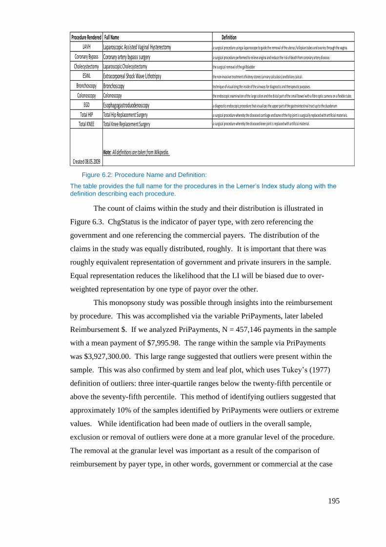
195
Figure 6.2: Procedure Name and Definition:
The table provides the full name for the procedures in the Lerner’s Index study along with the definition describing each procedure.
The count of claims within the study and their distribution is illustrated in
Figure 6.3. ChgStatus is the indicator of payer type, with zero referencing the
government and one referencing the commercial payers. The distribution of the
claims in the study was equally distributed, roughly. It is important that there was
roughly equivalent representation of government and private insurers in the sample.
Equal representation reduces the likelihood that the LI will be biased due to over-
weighted representation by one type of payor over the other.
This monopsony study was possible through insights into the reimbursement
by procedure. This was accomplished via the variable PriPayments, later labeled
Reimbursement $. If we analyzed PriPayments, N = 457,146 payments in the sample
with a mean payment of $7,995.98. The range within the sample via PriPayments
was $3,927,300.00. This large range suggested that outliers were present within the
sample. This was also confirmed by stem and leaf plot, which uses Tukey’s (1977)
definition of outliers: three inter-quartile ranges below the twenty-fifth percentile or
above the seventy-fifth percentile. This method of identifying outliers suggested that
approximately 10% of the samples identified by PriPayments were outliers or extreme
values. While identification had been made of outliers in the overall sample,
exclusion or removal of outliers were done at a more granular level of the procedure.
The removal at the granular level was important as a result of the comparison of
reimbursement by payer type, in other words, government or commercial at the case
Procedure Rendered Full Name Definition
LAVH Laparoscopic Assisted Vaginal Hysterectomy a surgical procedure using a laparoscope to guide the removal of the uterus,Fallopian tubes and ovaries through the vagina.
Coronary Bypass Coronary artery bypass surgery a surgical procedure performed to relieve angina and reduce the risk of death from coronary artery disease.
Cholecystectomy Laparoscopic Cholecystectomy the surgical removal of the gallbladder
ESWL Extracorporeal Shock Wave Lithotripsy the non-invasive treatment of kidney stones (urinary calculosis) and biliary calculi .
Bronchoscopy Bronchoscopy technique of visualizing the inside of the airways for diagnostic and therapeutic purposes.
Colonoscopy Colonoscopy the endoscopic examination of the large colon and the distal part of the small bowel with a fibre optic camera on a flexible tube.
EGD Esophagogastroduodenoscopy a diagnostic endoscopic procedure that visualizes the upper part of the gastrointestinal tract up to the duodenum
Total HIP Total Hip Replacement Surgery a surgical procedure whereby the diseased cartilage and bone of the hip joint is surgically replaced with artificial materials.
Total KNEE Total Knee Replacement Surgery a surgical procedure whereby the diseased knee joint is replaced with artificial material.
Note: All definitions are taken from Wikipedia.
Created 08.05.2009
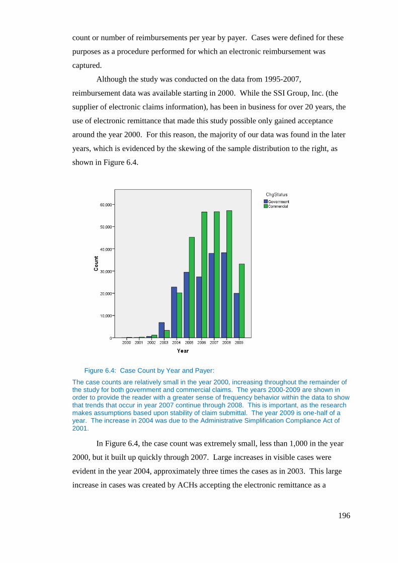
196
count or number of reimbursements per year by payer. Cases were defined for these
purposes as a procedure performed for which an electronic reimbursement was
captured.
Although the study was conducted on the data from 1995-2007,
reimbursement data was available starting in 2000. While the SSI Group, Inc. (the
supplier of electronic claims information), has been in business for over 20 years, the
use of electronic remittance that made this study possible only gained acceptance
around the year 2000. For this reason, the majority of our data was found in the later
years, which is evidenced by the skewing of the sample distribution to the right, as
shown in Figure 6.4.
Figure 6.4: Case Count by Year and Payer:
The case counts are relatively small in the year 2000, increasing throughout the remainder of the study for both government and commercial claims. The years 2000-2009 are shown in order to provide the reader with a greater sense of frequency behavior within the data to show that trends that occur in year 2007 continue through 2008. This is important, as the research makes assumptions based upon stability of claim submittal. The year 2009 is one-half of a year. The increase in 2004 was due to the Administrative Simplification Compliance Act of 2001.
In Figure 6.4, the case count was extremely small, less than 1,000 in the year
2000, but it built up quickly through 2007. Large increases in visible cases were
evident in the year 2004, approximately three times the cases as in 2003. This large
increase in cases was created by ACHs accepting the electronic remittance as a
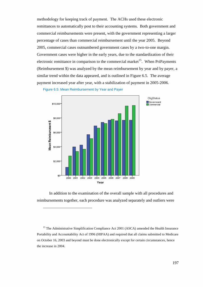
197
methodology for keeping track of payment. The ACHs used these electronic
remittances to automatically post to their accounting systems. Both government and
commercial reimbursements were present, with the government representing a larger
percentage of cases than commercial reimbursement until the year 2005. Beyond
2005, commercial cases outnumbered government cases by a two-to-one margin.
Government cases were higher in the early years, due to the standardization of their
electronic remittance in comparison to the commercial market15
. When PriPayments
(Reimbursement $) was analyzed by the mean reimbursement by year and by payer, a
similar trend within the data appeared, and is outlined in Figure 6.5. The average
payment increased year after year, with a stabilization of payment in 2005-2006.
Figure 6.5: Mean Reimbursement by Year and Payer
In addition to the examination of the overall sample with all procedures and
reimbursements together, each procedure was analyzed separately and outliers were
15 The Administrative Simplification Compliance Act 2001 (ASCA) amended the Health Insurance
Portability and Accountability Act of 1996 (HIPAA) and required that all claims submitted to Medicare
on October 16, 2003 and beyond must be done electronically except for certain circumstances, hence
the increase in 2004.
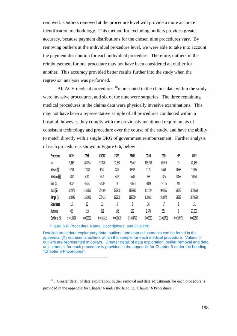
198
removed. Outliers removed at the procedure level will provide a more accurate
identification methodology. This method for excluding outliers provides greater
accuracy, because payment distributions for the chosen nine procedures vary. By
removing outliers at the individual procedure level, we were able to take into account
the payment distribution for each individual procedure. Therefore, outliers in the
reimbursement for one procedure may not have been considered an outlier for
another. This accuracy provided better results further into the study when the
regression analysis was performed.
All ACH medical procedures 16
represented in the claims data within the study
were invasive procedures, and six of the nine were surgeries. The three remaining
medical procedures in the claims data were physically invasive examinations. This
may not have been a representative sample of all procedures conducted within a
hospital; however, they comply with the previously mentioned requirements of
consistent technology and procedure over the course of the study, and have the ability
to match directly with a single DRG of government reimbursement. Further analysis
of each procedure is shown in Figure 6.6, below
Figure 6.6: Procedure Name, Descriptives, and Outliers:
Detailed procedure exploratory data, outliers, and data adjustments can be found in the appendix. (X) represents outliers within the sample for each medical procedure. Values of outliers are represented in dollars. Greater detail of data exploration, outlier removal and data adjustments for each procedure is provided in the appendix for Chapter 6 under the heading “Chapter 6 Procedures”.
16 . Greater detail of data exploration, outlier removal and data adjustments for each procedure is
provided in the appendix for Chapter 6 under the heading “Chapter 6 Procedures”.
Procedure LAVH CBYP CHOLX ESWL BRON COLO EGD HIP KNEE
(n) 9,143 141,054 52,120 12,532 22,467 118,253 61,019 75 40,483
Mean ($) 5730 12838 6142 4204 15945 1775 5640 14556 12496
Median ($) 3842 7044 4475 3205 5638 788 2375 10455 10260
min ($) -1024 -16050 -21264 0 -48614 -8443 -14116 247 1
max ($) 322971 1145851 354169 122910 1138980 611159 904256 59075 3878659
Range ($) 323995 1161901 375433 122910 1187594 619602 918372 58828 3878660
Skewness 15 10 12 6 8 36 17 2 151
Kurtosis 405 213 312 102 102 2,573 551 3 27,609
Outliers ($) x>=13804 x>=30692 X>=16312 X>=10639 X>=34755 X>=3069 X>=12701 X>=30972 X>=20507
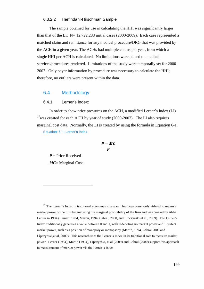
199
6.3.2.2 Herfindahl-Hirschman Sample
The sample obtained for use in calculating the HHI was significantly larger
than that of the LI: N= 12,722,238 initial cases (2000-2009). Each case represented a
matched claim and remittance for any medical procedure/DRG that was provided by
the ACH in a given year. The ACHs had multiple claims per year, from which a
single HHI per ACH is calculated. No limitations were placed on medical
services/procedures rendered. Limitations of the study were temporally set for 2000-
2007. Only payer information by procedure was necessary to calculate the HHI;
therefore, no outliers were present within the data.
6.4 Methodology
6.4.1 Lerner’s Index:
In order to show price pressures on the ACH, a modified Lerner’s Index (LI)
17was created for each ACH by year of study (2000-2007). The LI also requires
marginal cost data. Normally, the LI is created by using the formula in Equation 6-1.
Equation: 6-1: Lerner’s Index
P = Price Received
MC= Marginal Cost
17 The Lerner’s Index in traditional econometric research has been commonly utilized to measure
market power of the firm by analyzing the marginal profitability of the firm and was created by Abba
Lerner in 1934 (Lerner, 1934, Martin, 1994, Cabral, 2000, and Lipczynski et al., 2009). The Lerner’s
Index traditionally generates a value between 0 and 1, with 0 denoting no market power and 1 perfect
market power, such as a position of monopoly or monopsony (Martin, 1994, Cabral 2000 and
Lipczynski,et al, 2009). This research uses the Lerner’s Index in its traditional role to measure market
power. Lerner (1934), Martin (1994), Lipczynski, et al (2009) and Cabral (2000) support this approach
to measurement of market power via the Lerner’s Index.

200
Here, P is the price received within the market for the good, and MC is the
marginal cost associated with producing the good. The LI also provides a measure of
the monopoly power of each ACH. The LI traditionally provides an index from zero
to one, with one being true monopoly power, and zero possessing no monopoly
power. This is achieved, as, marginal cost (MC) equals price under perfect
competition. Effectively, the formula becomes price minus price under perfect
competition, as a proportion of price.
In this case, an adaptation of the LI was valuable to address concerns in the
previous research of Shibata (1973), Pauly (1998), Feldmand (2001), and Taylor
(2003), that ACHs are monopolistic in that the lower prices paid for services are a
function of monopoly busting and not a condition of monopsony. By utilizing the LI,
one can answer two questions: 1) what, if any, are the price pressures on ACHs (are
they price makers or price takers)? 2) Is there any concern of a monopoly power still
prevalent with ACHs? By analyzing price pressures, one is able to understand
whether ACHs are price takers or price makers within the market.
As market power for ACHs is bounded geographically, the research
considered the geographically bounded market power in order to reduce the likelihood
of misrepresenting market power due to the distortion of the geographically bounded
markets. A problem with creating the LI for each hospital for each of the years
studied was that marginal cost data was not provided via the MCR. Therefore,
another method was used to obtain access to cost data. This approach provided an
approximate value of the LI. This modified LI provided valuable information and
insight into market power of hospitals. In order to calculate the modified LI, the
average total cost was used instead of the marginal cost.
The average total cost (ATC) per procedure was calculated by taking the total
operating expenses provided in the MCR for each ACH per year, and dividing that by
the total number of inpatient and outpatient days provided by the ACH that year
which provided the average cost per patient day (ACPPD) for the ACH. The ACPPD
is then multiplied by the geometric length of stay (GMLOS). However, total
operating costs include depreciation and interest expenses along with general and
administrative expenses. These additional expenses can be regarded as fixed costs.
Therefore, in taking the ATC to equal the MC, we assume that the ATC= average
variable costs (AVC) (that is, the average fixed costs are close to zero), and that the

201
AVC are constant with respect to output (patient days) at output ranges observed in
practice. The ATC per procedure is represented in Equation 6-2. This is the fully
burdened cost of providing services to a patient per day. The ACHs utilize the total
cost per patient days to measure the productivity and efficiency of the firm.
Equation: 6-2: Average Total Cost Per Procedure
(
)
C = Avg. Total Cost (ATC)
j = procedure
E = Total Annual Operating Expenses
D= Total inpatient and outpatient days
g = Geometric Length of Stay
i = firm
t = Year
Each of the nine procedures outlined within the study were reimbursed by the
government utilizing a DRG. Each DRG is assigned a Geometric Mean Length of
Stay (GMLOS)18
, which is the geometric mean length of stay in days for that
particular procedure or diagnosis. Through studies, the government has determined
the GMLOS to be the amount of time for a patient to be in the hospital with each
particular procedure or illness treated, weighted by frequency of the number of days.
The commercial insurers also utilize this same geometric length of stay in order to
determine reimbursements, as well as to determine whether scrutiny of a claim is
necessary. In other words, this process is utilized to determine the appropriate length
of patient stay for the commercial and government payor alike.
An assumption made in this research was that the ACH incurs the geometric
length of stay cost of treating the patients. This assumed that a patient with a given
DRG actually stayed in the hospital the amount of time noted by the GMLOS. When
18 A table outlining the Geometric Length of Stay for each procedure and date range is provided in
The Appendix. This GMLOS provided for each procedure is listed in days. The date ranges
correspond to the time period of this research.

202
the actual patient time in the hospital differed from GMLOS, it is likely that the ATC
will not equal the average cost (AC).
The geometric length of stay is measured in patient days. Therefore, the AC
per patient day multiplied by the geometric length of stay for a specific procedure
equals the ATC for a given procedure. The ATC was calculated for each procedure
within the study by using the preceding equation, Equation 6-2. The ATC for each
procedure was calculated, and the approximation of the LI was created using the
formula in Equation 6-3.
Equation: 6-3: Lerner’s Index (Modified)
∑
(
)
L = Proxy for the Lerner’s Index
P= Price paid by the insurer
C= Average Total Cost (ATC)
i = individual ACH
t = year
j= procedure
n = total number of procedures within (t) for ACH (i)
By using the ATC, a modified LI was calculated for each claim within the
study, for a total of 273,399 LIs. The LIs were then summed by year and ACH, and
divided by the total number of procedures conducted in the study by the ACH for a
given year. This calculation yielded an average LI for each ACH for each year it
participated within the study. Using this methodology, 1,603 LIs were produced.
6.4.1.1 Lerner’s Index Hypotheses:
This research examined the lack of market power on behalf of ACHs in the
healthcare market, and its negative consequence for decisions of capital structure. In
order for the research to proceed under this premise, two conditions must be evident:
1) The LI values must be low to show lack of market power; and 2) The LI values
must positively correlate with the Real FCF. The hypothesis for this examination is
found in Hypothesis 6-6.
Pauly (1988) proposed that monopsony market power was a possibility given
the constructs of the U.S. healthcare market. He proposed that monopsony within this
market may not be beneficial from the supplier or consumer’s perspective, as it most
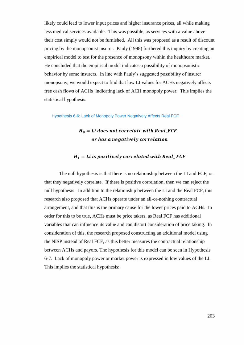
203
likely could lead to lower input prices and higher insurance prices, all while making
less medical services available. This was possible, as services with a value above
their cost simply would not be furnished. All this was proposed as a result of discount
pricing by the monopsonist insurer. Pauly (1998) furthered this inquiry by creating an
empirical model to test for the presence of monopsony within the healthcare market.
He concluded that the empirical model indicates a possibility of monopsonistic
behavior by some insurers. In line with Pauly’s suggested possibility of insurer
monopsony, we would expect to find that low LI values for ACHs negatively affects
free cash flows of ACHs indicating lack of ACH monopoly power. This implies the
statistical hypothesis:
Hypothesis 6-6: Lack of Monopoly Power Negatively Affects Real FCF
The null hypothesis is that there is no relationship between the LI and FCF, or
that they negatively correlate. If there is positive correlation, then we can reject the
null hypothesis. In addition to the relationship between the LI and the Real FCF, this
research also proposed that ACHs operate under an all-or-nothing contractual
arrangement, and that this is the primary cause for the lower prices paid to ACHs. In
order for this to be true, ACHs must be price takers, as Real FCF has additional
variables that can influence its value and can distort consideration of price taking. In
consideration of this, the research proposed constructing an additional model using
the NISP instead of Real FCF, as this better measures the contractual relationship
between ACHs and payors. The hypothesis for this model can be seen in Hypothesis
6-7. Lack of monopoly power or market power is expressed in low values of the LI.
This implies the statistical hypothesis:
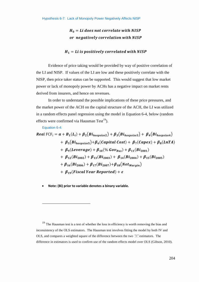
204
Hypothesis 6-7: Lack of Monopoly Power Negatively Affects NISP
Evidence of price taking would be provided by way of positive correlation of
the LI and NISP. If values of the LI are low and these positively correlate with the
NISP, then price taker status can be supported. This would suggest that low market
power or lack of monopoly power by ACHs has a negative impact on market rents
derived from insurers, and hence on revenues.
In order to understand the possible implications of these price pressures, and
the market power of the ACH on the capital structure of the ACH, the LI was utilized
in a random effects panel regression using the model in Equation 6-4, below (random
effects were confirmed via Hausman Test19
).
Equation 6-4:
( ) ( ) ( )
( )
( )
Note: (Bi) prior to variable denotes a binary variable.
19 The Hausman test is a test of whether the loss in efficiency is worth removing the bias and
inconsistency of the OLS estimators. The Hausman test involves fitting the model by both IV and
OLS, and compares a weighted square of the difference between the two estimators. The
difference in estimators is used to confirm use of the random effects model over OLS (Gibson, 2010).

205
The model provided an estimate of the strength and relationship of market
power measured in the LI and the real FCFs (FCF measured in real [1996] terms).
This relationship allowed for a better understanding of the real FCF created by the
market power of the ACH, and gave the research insight into the considerations of
managers who decide the capital structures of the ACHs. In addition, a second model
was constructed, with the LI as the primary independent variable and Net Income
from Service to Patients (NISP) as the dependent variable, as shown in Equation 6-5.
The additional model was to examine LI in relation to the NISP. The change to
utilizing the NISP was because the real FCF can be distorted by the variable Other
Income in the MCR. Other Income is the sources of income other than revenue from
service to patients, and was defined in Chapter 3. The NISP encompassed all revenue
streams derived from insurance reimbursement, and would better reflect monopoly
power or lack thereof, in relation to the payors. In other words, if ACHs are
monopolist and can obtain a higher price margin and therefore have a higher LI, then
this should be evident in the revenues derived from that monopoly power. Likewise,
if ACHs lack monopoly power and have low LIs, this too should be more evident in
the relationship with NISP.
The NISP was a better measure than Real FCF for price taker status because
the revenue stream was supported largely by payor reimbursement. The NISP is
defined as Net Patient Revenues minus Total Operating expenses. Net Patient
Revenues is defined as Total Patient Revenues minus Contractual Allowances. Total
Patient Revenues is defined from sources such as inpatient care, outpatient care,
ancillary services, home health, ambulance, outpatient rehab, ASC and hospice. It
was evident that the services included in NISP captures all revenue streams for which
insurance reimbursement is likely. The NISP is included in net income calculation in
the MCR; therefore, it affects the calculation of FCFs, and likewise, Real FCFs. If
lower Real FCFs affect capital structure, a low value of the LI and positive correlation
in the LI and NISP provide evidence of two things: price taker status for services to
patients and the lack of monopoly power on the part of the ACH for services to
patients, thus providing an alternative to examining monopoly power with just the
relationship of the LI and Real FCFs.
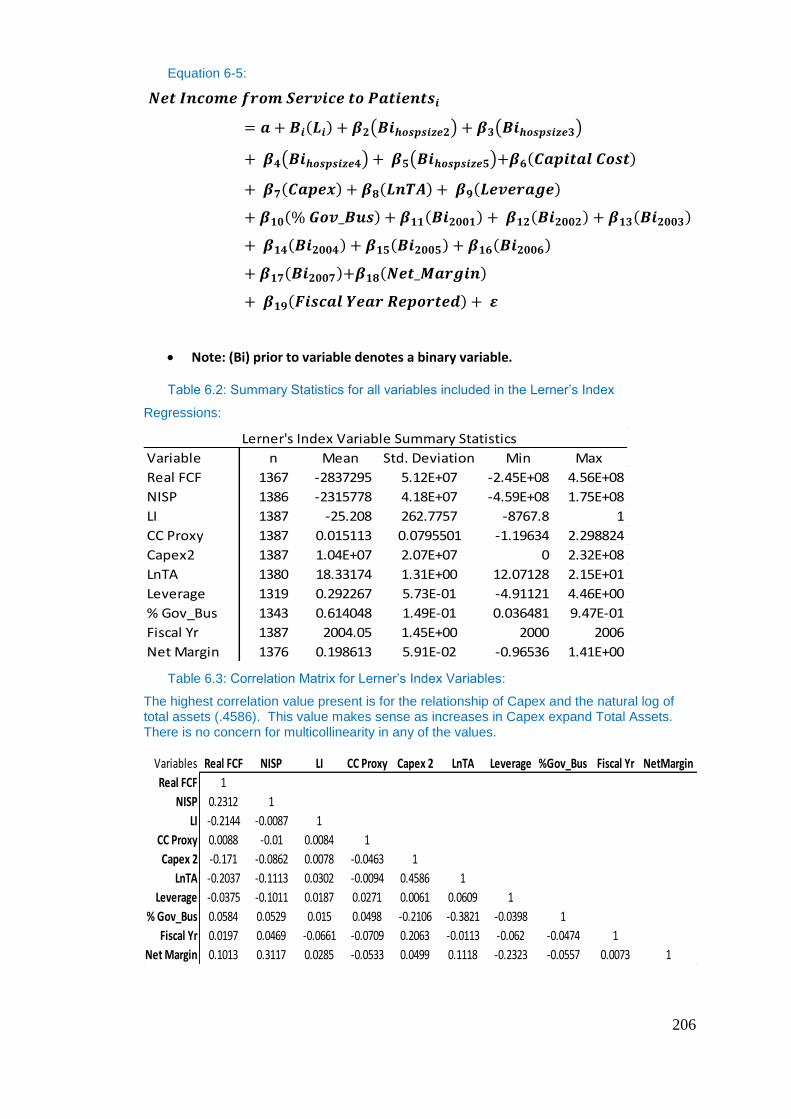
206
Equation 6-5:
( ) ( )
( ) ( )
Note: (Bi) prior to variable denotes a binary variable.
Table 6.2: Summary Statistics for all variables included in the Lerner’s Index
Regressions:
Table 6.3: Correlation Matrix for Lerner’s Index Variables:
The highest correlation value present is for the relationship of Capex and the natural log of total assets (.4586). This value makes sense as increases in Capex expand Total Assets. There is no concern for multicollinearity in any of the values.
Lerner's Index Variable Summary Statistics
Variable n Mean Std. Deviation Min Max
Real FCF 1367 -2837295 5.12E+07 -2.45E+08 4.56E+08
NISP 1386 -2315778 4.18E+07 -4.59E+08 1.75E+08
LI 1387 -25.208 262.7757 -8767.8 1
CC Proxy 1387 0.015113 0.0795501 -1.19634 2.298824
Capex2 1387 1.04E+07 2.07E+07 0 2.32E+08
LnTA 1380 18.33174 1.31E+00 12.07128 2.15E+01
Leverage 1319 0.292267 5.73E-01 -4.91121 4.46E+00
% Gov_Bus 1343 0.614048 1.49E-01 0.036481 9.47E-01
Fiscal Yr 1387 2004.05 1.45E+00 2000 2006
Net Margin 1376 0.198613 5.91E-02 -0.96536 1.41E+00
Variables Real FCF NISP LI CC Proxy Capex 2 LnTA Leverage %Gov_Bus Fiscal Yr NetMargin
Real FCF 1
NISP 0.2312 1
LI -0.2144 -0.0087 1
CC Proxy 0.0088 -0.01 0.0084 1
Capex 2 -0.171 -0.0862 0.0078 -0.0463 1
LnTA -0.2037 -0.1113 0.0302 -0.0094 0.4586 1
Leverage -0.0375 -0.1011 0.0187 0.0271 0.0061 0.0609 1
% Gov_Bus 0.0584 0.0529 0.015 0.0498 -0.2106 -0.3821 -0.0398 1
Fiscal Yr 0.0197 0.0469 -0.0661 -0.0709 0.2063 -0.0113 -0.062 -0.0474 1
Net Margin 0.1013 0.3117 0.0285 -0.0533 0.0499 0.1118 -0.2323 -0.0557 0.0073 1

207
Variable Definitions:
LI- (Lerner’s Index) was the primary independent variable and is a
measurement of market power of ACHs. Given the premise that monopsony by
payers exists within the healthcare market, and that ACHs presented as lacking
market power, we expected the Lerner’s Index, a measurement for market power, for
each ACH to have a strong positive correlation with the Real FCFs of ACHs and
NISP of ACHs. The lack of market power on behalf of ACHs was the primary reason
for the expectation of ACHs to be price takers. Therefore, a low value of a LI will
equate to a low Real FCF and NISP. There are limitations in the use of the LI in this
case as the LI is a modified LI, which uses average total cost instead of marginal
costs. However, it is assumed that ATC equals the MC, that ATC equals the average
variable costs (AVC) (that is, the average fixed costs are close to zero), and that AVC
are constant with respect to output (patient days) at output ranges observed in
practice.
Leverage – (Leverage) was used to measure the outstanding debt of the ACH.
Leverage is defined as total long-term liabilities divided by total assets. This is
included in the regressions to control for the effect Leverage has on Real FCFs. As
hospitals are heavily leveraged, inclusion of the variable allows the regression to
control for any effects or explanation it might have on Real FCFs. Leverage was
expected to have a negative correlation with Real FCFs. As leverage increases,
borrowing costs associated with leverage increase, thereby reducing FCFs. Leverage
was used to control for the amount of debt of an ACH. Leverage is a calculated
variable within the data. A definition for the variable can be found in the appendix for
Chapter 4 variable nomenclature and definitions. There were no limitations in
calculating the variable from the data.
Profitability – (Net Margin) was included as the control for profitability while
observing the relation between real FCF and LI. Profitability of the ACH affects the
generation of Real FCFs and therefore its inclusion in the regression as a control
variable is important. Net Margin has been deflated using the CPI for hospital
services (1996-2007; U.S. Bureau of Labor Statistics 2009). Net Income iis a primary
variable in calculating Net Margin; it therefore has and impact on the ability of an
ACH to generate free cash flows. Net Income is comprised of two revenue streams
208
for ACHs Net Income from Service to Patients and Other Income. Profitability was
expected to have a positive correlation with Real FCFs.
Size – (LnTA) the natural log of total assets used as a control for size in the
research. This logic followed previous research in its utilization to control for size.
Controlling for size takes into account the magnitude and production capability of the
ACH when looking at real FCFs and its relation to the LI. Total Assets is a variable
provided within the MCR. Total Assets has been deflated by the CPI for hospital
services (1996-2007; U.S. Bureau of Labor Statistics 2009).
In addition to LnTA, a binary variable was used to represent the size
categories created in Chapter 3. Four out of the five categories were represented by a
binary variable. Size was expected to have a positive correlation with Real FCF’s and
NISP. As assets increase, so too does the production capability of the ACH. There is
a limitation in using a binary size variable which is based upon licensed beds as
ACHs may not have all the licensed beds in production at all times which may cause
this variable to slightly overstate their production capabilities. The concern is
somewhat reduced as ACHs can quickly put these beds back in to production should
demand require it.
Time - (t) Fiscal year was the control for time. Its inclusion was to reduce
temporal effects within the model caused by time. Fiscal year is a provided variable
within the MCR. Time was controlled for by the inclusion of a binary variable for
each year of the study minus one. Therefore, while the data covered the years 2000-
2007, only 2001-2007 had a binary variable. Time was expected to have a positive
correlation with the Real FCFs and NISP as revenues are expected to increase slightly
with inflation and increasing costs.
Real FCF- (Real FCF) The Real FCF was the free cash flow of each ACH in
1996 dollars. It is the dependent variable in both the regression for the Lerner’s Index
and the Herfindahl-Hirschman Index. Free cash flows were presented in 1996 dollars
in order to remove changes in the FCF due to inflation during the longitudinal period
of this study. It is expected that Real FCF will have a negative correlation with the
Lerner’s Index and Herfindahl-Hirschman Index. A limitation in the use of Real FCF
comes from the underlying issues in calculating FCFs. As was mentioned previously
FCF is missing data on total depreciation and capital expenditures. The majority of
cases within the MCR data were missing both of these variables. Where both data
209
components are missing FCF may be may be slightly understated. It should also be
noted that free cash flows are calculated using net income as a starting point. Net
income is comprised of net income from services to patients (NISP) and other income.
While margins calculated using only the net income from service to patients were
negative for the time period of this study, margins calculated using both NISP and
Other Income were positive. This suggests that other income provides the necessary
revenues for ACHs to have positive margins overall. As the Lerner’s Index in this
research is a measure of margin on selected health services, it may present a problem
in the expected correlation between the LI and Real FCF’s.
Individual ACH – (i) was the individual ACH for which the all the variables
pertain.
Capital Expense - (Capex2) Capex2 was used as the control mechanisms for
the uses of free cash flow and leverage in acquiring assets. This allowed the model to
account for ACH free cash flow in light of capital spending. Capex was a calculated
variable that represented the change between old (time t-1) capital assets and new
capital assets (time t) as used in calculating the FCF and mentioned previously.
Capital expense was expected to have a negative relation with Real FCFs. Any
increase in Capex decreases the amount of FCFs available to the ACH. The use of
Capital Expense is limited by the number of cases, which originally contained value
for old and new capital assets. Where the data was missing, a zero was added. This
may cause the capital expenditures of ACHs to be over or under stated.
Cost of Capital - (CCProxy) was used in the study to control for cost of
capital associated with the size of debt. The study made an assumption that firms
with similar debt sizes would differentiate their use of cash flows when servicing debt
if the firms had different costs of capital. Taking total interest expense as a ratio to
total long-term liabilities created a proxy for cost of capital. One would expect that
similar to leverage, the cost of capital would negatively correlate to the FCF. The
basis for this is that the FCF is computed after all cash flows for maintenance of
leverage and short-term liabilities have been paid. The more it costs to maintain the
debt of an ACH, the more it reduces the FCF. Including this variable accounts for all
Real FCF fluctuation due to debt, both Leverage and its costs. A limitation in the
variable CCProxy is generated by the possibility of long term liabilities on the balance
210
sheet not requiring any interest to be paid. Where this is the case, it is likely that CC
Proxy is understated.
Percent of Government Business – (%Gov_Bus) was used within the study
to control for the amount of business an ACH receives from government payors.
Government payors typically pay less than private ones. The calculation for this
variable was provided in Chapter 4. Percent government business also controlled for
agency cost by taking into account the amount of the Real FCFs derived from the
government, and %Gov_Bus will have a negative correlation to the real FCFs, as per
Chapter 4. Limitations of the Percent of Government Business were fully discussed
in Chapter 4; these were generated by the difference in reimbursement between
government and private payors. In this case the government reimburses ACHs less for
a given patient days services, therefore it is likely that because the proxy is based
upon the use of patient days consumed by the government of total patient days
rendered by the ACHs, the proxy will overstated the revenues derived from
government sources. The said the proxy does capture the amount of resources
consumed by the government as ACHs output is measured in patient days.
Net Income from Service to Patients- (NISP) was the net income from
service to patients, comprised of net patient revenues minus total operating expenses.
The NISP was presented in 1996 dollars in order to remove influence in NISP due to
inflation during the longitudinal period. NISP was included as the dependent variable
in a subsequent Lerner’s Index model to analyze the correlation of the Lerner’s Index
with those revenues derived solely from services rendered to patients where
reimbursement was from the payors. This was done to exclude any distortion Other
Income may have had on the model analyzing LI with Real FCFs. It also provided a
better way for modeling price taking by ACH’s in comparison to payors.
6.4.2 Herfindahl Hirschman Index:
While the LI provided value in understanding price pressures that ACHs are
under and the possibly monopoly power that exist for ACHs (the suppliers) in their
markets, an additional understanding of market power contained within the payors
(the consumer or buyer) side of the market was required. While the research was not
able to measure the market power for the payor directly, it was able to achieve
measurement via use of an alternative approach. This alternative approach allowed the

211
research to infer a value for market power via The New Empirical Industrial
Organization (NEIO). While the NEIO model will be discussed later in more detail,
an important variable used to achieve this inference must be created and measured as
it provides the basis of the research to move forward under the NEIO model. The
research utilizes this alternative methodology using the NEIO by measuring
concentration of payors in the market faced by ACHs via the Herfindahl Hirschman
Index (HHI)20
. Measuring concentration of payors allowed the research to examine
concentrations effect on free cash flows via regression analysis possibly providing
evidence of collusive behavior. By combining concentration, collusion and demand
elasticity for the market of healthcare services the model seeks to infer a value for the
market power of the payors, which supports collusive monopsony.
Evidence of collusive monopsony was created in three basic steps: The
primary base to support collusive monopsony was the calculation of the HHI, which
measured concentration ofthe payor market faced by ACHs. The HHI value
supported concentration via its numerical value in comparison to that of acceptable
values applied by the U.S. Department of Justice for other instances of market power.
Secondly, concentration via the HHI was analyzed to observe its influence on Real
FCFs of ACHs to provide evidence of collusion of government and commercial
payors via random effects panel regression. Thirdly, using evidence of collusion, the
research combined both the concentration of the payor market via the HHI, an
estimate of demand elasticity for healthcare services and evidence of collusion via the
regression analysis into the NEIO to estimate the market power of the payor.
20 The Herfindahl-Hirschman Index is and index used to measure concentration of a market by
looking as the size of firms market share in relation to industry as an indicator of the competition
amongst them (Miller, 1982, Cahen and Sullivan, 1984 and Rhodes, 1993). Orris Herfindahl and
Albert Hirschman created the Herfindahl-Hirschman Index. It is widely used as an econometric
concept in competition or antitrust law. The HHI takes the sum of the squares of the market shares of
the 50 largest firms within an industry. This formula provides an average market share weighted by
market share. It provides a measurement from 0 to 1.0 with 0 representing large competition and 1
representing monopolistic or monopsonistic power. The HHI is often express as the value between 1
and 0 multiplied by 10,000. The use of this methodology is similar in approach to Hersch (1994).
Schramm and Renn (1984).

212
In order to proceed, an understanding of the HHI is necessary. The HHI is
defined by the U.S. Department of Justice and the Federal Trade Commission as:
“The HHI takes into account the relative size and distribution of the firms in a
market and approaches zero when a market consists of a large number of firms
of relatively equal size. The HHI increases both as the number of firms in the
market decreases and as the disparity in size between those firms increases.
Markets in which the HHI is between 1000 and 1800 points are considered to
be moderately concentrated and those in which the HHI is in excess of 1800
points are considered to be concentrated. Transactions that increase the HHI
by more than 100 points in concentrated markets presumptively raise antitrust
concerns under the Horizontal Merger Guidelines issued by the U.S.
Department of Justice and the Federal Trade Commission.” (DoJ, 2009)
The HHI is the best measurement due to its ability to indicate level of market
concentration similar to methodologies employed by Seth (2006). In Seth’s research,
the index measured concentration amongst health insurers and its effects upon
physician earnings and services. Similarly, in this study, the HHI measured the
concentration of insurers within the ACH market and its effects on the free cash flows
of ACHs. A problem that arises when using the HHI as a measurement within
healthcare is the geographically different markets of ACHs. Insurers/payers often are
restricted from crossing state lines, making it difficult to compete in a broad
geographic area. Therefore, ACHs face different competitive markets of insurers,
which vary according to location.
In order to overcome this estimation problem, buyer side concentration must
be analyzed by each individual ACH geographic region. This was accomplished by
taking the payer for each claim by ACH and Year, which was available within the
claims/remit database, and calculating the market share that the payer possessed out
of the total number of procedures of the ACH within the study that year. Then, this
value was squared and summed by ACH and year. The HHI formula is listed below
in Equation 6-6.
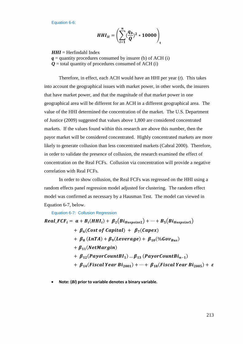
213
Equation 6-6:
(∑
)
HHI = Herfindahl Index
q = quantity procedures consumed by insurer (b) of ACH (i)
Q = total quantity of procedures consumed of ACH (i)
Therefore, in effect, each ACH would have an HHI per year (t). This takes
into account the geographical issues with market power, in other words, the insurers
that have market power, and that the magnitude of that market power in one
geographical area will be different for an ACH in a different geographical area. The
value of the HHI determined the concentration of the market. The U.S. Department
of Justice (2009) suggested that values above 1,800 are considered concentrated
markets. If the values found within this research are above this number, then the
payor market will be considered concentrated. Highly concentrated markets are more
likely to generate collusion than less concentrated markets (Cabral 2000). Therefore,
in order to validate the presence of collusion, the research examined the effect of
concentration on the Real FCFs. Collusion via concentration will provide a negative
correlation with Real FCFs.
In order to show collusion, the Real FCFs was regressed on the HHI using a
random effects panel regression model adjusted for clustering. The random effect
model was confirmed as necessary by a Hausman Test. The model can viewed in
Equation 6-7, below.
Equation 6-7: Collusion Regression
( ) ( )
Note: (Bi) prior to variable denotes a binary variable.
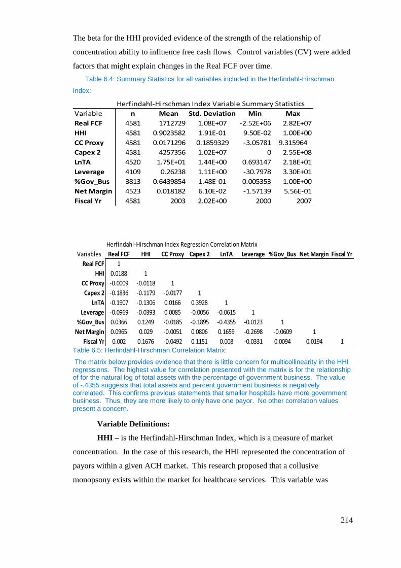
214
The beta for the HHI provided evidence of the strength of the relationship of
concentration ability to influence free cash flows. Control variables (CV) were added
factors that might explain changes in the Real FCF over time.
Table 6.4: Summary Statistics for all variables included in the Herfindahl-Hirschman
Index:
Table 6.5: Herfindahl-Hirschman Correlation Matrix:
The matrix below provides evidence that there is little concern for multicollinearity in the HHI regressions. The highest value for correlation presented with the matrix is for the relationship of for the natural log of total assets with the percentage of government business. The value of -.4355 suggests that total assets and percent government business is negatively correlated. This confirms previous statements that smaller hospitals have more government business. Thus, they are more likely to only have one payor. No other correlation values present a concern.
Variable Definitions:
HHI – is the Herfindahl-Hirschman Index, which is a measure of market
concentration. In the case of this research, the HHI represented the concentration of
payors within a given ACH market. This research proposed that a collusive
monopsony exists within the market for healthcare services. This variable was
Herfindahl-Hirschman Index Variable Summary Statistics
Variable n Mean Std. Deviation Min Max
Real FCF 4581 1712729 1.08E+07 -2.52E+06 2.82E+07
HHI 4581 0.9023582 1.91E-01 9.50E-02 1.00E+00
CC Proxy 4581 0.0171296 0.1859329 -3.05781 9.315964
Capex 2 4581 4257356 1.02E+07 0 2.55E+08
LnTA 4520 1.75E+01 1.44E+00 0.693147 2.18E+01
Leverage 4109 0.26238 1.11E+00 -30.7978 3.30E+01
%Gov_Bus 3813 0.6439854 1.48E-01 0.005353 1.00E+00
Net Margin 4523 0.018182 6.10E-02 -1.57139 5.56E-01
Fiscal Yr 4581 2003 2.02E+00 2000 2007
Herfindahl-Hirschman Index Regression Correlation Matrix
Variables Real FCF HHI CC Proxy Capex 2 LnTA Leverage %Gov_Bus Net Margin Fiscal Yr
Real FCF 1
HHI 0.0188 1
CC Proxy -0.0009 -0.0118 1
Capex 2 -0.1836 -0.1179 -0.0177 1
LnTA -0.1907 -0.1306 0.0166 0.3928 1
Leverage -0.0969 -0.0393 0.0085 -0.0056 -0.0615 1
%Gov_Bus 0.0366 0.1249 -0.0185 -0.1895 -0.4355 -0.0123 1
Net Margin 0.0965 0.029 -0.0051 0.0806 0.1659 -0.2698 -0.0609 1
Fiscal Yr 0.002 0.1676 -0.0492 0.1151 0.008 -0.0331 0.0094 0.0194 1

215
included in the regressions as it allowed the research to analyze the effect
concentration has on the real free cash flows of ACHs. Concentration affecting free
cash flows negatively provides evidence of collusion. As collusion was expected,
concentration, or the HHI, will have negative correlation with Real FCFs.
Concentration of the payor market would not have a negative impact on the Real
FCFs if collusion was not present. Concentration was calculated using the payor
count that a hospital submits electronically. Where this deviates from the actual
number of payors that an ACH submits bills to in any format, will cause the
concentration measurement to skew, with an overstatement of concentration being the
most likely. In order to control for this likelihood the research structures the models
and set limits within each model for the least amount of payors a hospital could
submit electronically. For instance, in the models the least amount of payors that an
ACH was allowed to submit electronically ranged from 7 in one model to 1 in
another. As the least allowable payor count approaches one, the model is more likely
to have error due to overstatement of concentration. Payor count was also controlled
for via direct variable inclusion within the model.
Payor Count - Payor Count was controlled for, as ACHs may have multiple
payors. The number of payors can affect real free cash flows. A binary variable was
created for each payor count up to 50. All payor counts above 50 were included in
one variable. An n-1 strategy was followed, meaning that there was one less binary
for the number of payor counts included in the model. Payor count was calculated
directly from the claims data by counting the exact number of different payors that an
ACH submitted bills electronically for. It was included also to account for the
variability in payment that comes with an increase in the number of payors. This is
important and most payors differ on reimbursement of the same procedure or health
service.
All other variables used in the HHI analysis have the same definitions as
described in the LI analysis.
6.4.2.1 Hypothesis for Collusive Monopsony Power based on the
Herfindahl Hirschman Index:
The null hypothesis is that there is no collusion; therefore, the HHI does not
have a negative correlation with Real_FCF. If the HHI does not correlate with Real

216
FCFs, then concentration does not affect the Real FCFs of ACHs, and therefore no
evidence of collusion can be shown. Likewise, if the HHI has a positive correlation
with Real FCFs, then concentration is having a positive effect on Real FCFs. In other
words, the more concentrated the insurer market faced by the ACH, the more the
ACH Real FCFs increase. Both of these situations undermine the presence of
collusion by the payors. However, the null hypothesis can be rejected if a negative
correlation is found, as this provides evidence of collusion. In this case, the presence
of collusion indicates that the payors are using market power to affect prices paid to
ACHs The interaction of concentration and collusion with market power via NEIO
are discussed in greater detail in Section 6.5.2.3. A negative correlation between
Real_FCF and HHI was expected, as per previous literature (Seth 2006). This
implies the statistical hypothesis:
Hypothesis 6-8: Collusion Hypothesis
6.4.3 Expected Results
The combination of the LI and the HHI allowed analysis through the research
to determine whether collusive monopsony is present. Based upon previous research,
the model will provide evidence of lower values for the LI of ACHs, indicating low
market power for ACHs. The low market power of ACHs will show and affect
capital structure via the FCF, and likewise, there will be positive correlation of the LI
of ACHs with the NISP and Real FCF, indicating that ACHs are price takers, as the
ACHs will be unable to demand prices paid. Thus, FCFs will suffer and will be
reduced. The reduction of FCFs will limit access to debt markets, as less FCFs will
be available to be promised to pay principle and interest on loans from borrowers.
This limitation on debt will change the way ACHs’ managers approach the capital
structures of their organizations. Additionally, measuring concentration through the
HHI of the ACH payor market will provide evidence of high concentration of the
ACH payor market, and that the higher concentration of the ACH payor market will
217
have negative effects upon free cash flows, indicating collusion in ACH markets with
concentrated markets. It is only by use of market power that concentration negatively
affects FCFs of ACHs. Concentrations negatively affecting FCFs suggest collusion.
Collusion provides the framework by which market power expresses itself.
Feldmand and Wholey (2001) suggested that lower reimbursement indicated
that conditions within the U.S. healthcare market were those of monopoly busting and
not of monopsony. If the conditions within the market were those of monopoly
busting, then one would expect to find that the HHI calculated for the payors has no
affect upon FCFs, and therefore, there is no evidence of collusion. In addition, one
would expect the LI (on behalf of the ACHs) to show evidence of market power. One
also would expect ACHs to be price makers, or at least not price takers within the
market. If a low value was found for the LI (on behalf of the ACH), this would
evidence a lack of monopoly power. Thus, ACHs as price takers would suggest that
payors are exploiting market power.
6.5 Results
6.5.1 Monopsony Results Using the Lerner’s Index
In an attempt to uncover market power on the part of ACHs, the LI was
calculated on behalf of the ACH. Calculating the LI for the ACH enabled the
researcher to analyze two questions within one calculation. The first was, is there
monopoly power on the part of the hospital? Thus alleviating the concerns expressed
in the research of Feldman and Wholey (2001). If the hospital had monopoly power,
then it would be reflected by a high LI. If however a low value for the LI was found,
then this would provide the research with the ability to refute the findings of Felman
and Wholey (2001). Feldman and Wholey (2001) had suggested that lower
reimbursement to hospitals by HMOs represented a breakup of monopoly power of
the ACH rather than traditional monopsony by the HMOs. The second question is if
ACHs are price takers. If ACHs are price takers then they will not be able to
determine prices paid for healthcare services rendered to patients. ACHs are more
likely to be price takers under a collusive monopsony as business terms are dictated
by the all or nothing contractual arrangement.

218
Figure 6.13: Lerner’s Index Descriptives by Fiscal Year:
All mean value of the LI is negative for all years. While there is some variation in the value of the mean LI over time, the values have a declining trend. This suggests that market power of ACHs was declining over the time presented in this study. This is supported via median values for the LI, which are also negative for all years, and they exhibit negative trending over time.
Observing mean values for the LI found in Figure 6.13, large negative values
were present in all years. While negative LI values normally are not considered a
possibility, two conditions allowed this to occur: One is that this LI used average
total costs, rather than marginal costs. The second is that low reimbursement by
payers is not enough to cover costs, whether marginal or average. Median values also
were negative in every year of the longitudinal study. These mean and median values
supported a lack of market power by ACHs because the LI is calibrated in such a way
that if the ACHs had market power, then the LI values would have approached one,
and one is a monopoly condition. The evidence provided in the low LI values
suggests that ACHs lack monopoly power. The lack of monopoly power affects on
capital structure via the FCF is analyzed in Model 1, and price-taking status is
analyzed in Model 2 by way of relationship with the NISP.
6.5.1.1 Lerner’s Index Correlation with Free Cash Flows
Two models were constructed for use with the ACH LI. Each regression was
conducted using random effects panel data regression. A Hausman Test confirmed
the use of the random effects model. Standard errors were adjusted for clustering
within each model based upon the case identifier (prv_num). This corrected the
model for the assumption that each value with the variable was independent of every
other value for the same case. In each model, the LI was used as the primary
independent variable.
In the first model, the Real FCFs were regressed upon the LI. Control
variables included size, capital cost, capital expenditures, leverage, amount of
government business, and time. Additional binary variables were included as control
variables for size and time.
Lerner's Index Values
Year 2000 2001 2002 2003 2004 2005 2006 2007
Mean -3.3886 -5.4785 -5.347 -6.8187 -6.342 -6.4891 -6.9472 -6.7088
Median -1.79 -2.68 -3.15 -4.81 -4.94 -4.94 -5.64 -5.69
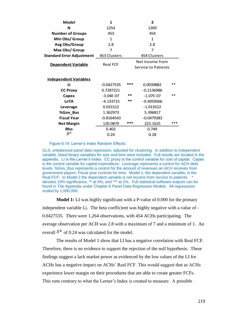
219
Figure 6.14: Lerner’s Index Random Effects:
GLS, unbalanced panel data regression, adjusted for clustering. In addition to independent variable, listed binary variables for size and time were included. Full results are located in the appendix. LI is the Lerner’s Index. CC proxy is the control variable for cost of capital. Capex is the control variable for capital expenditure. Leverage represents a control for ACH debt levels. %Gov_Bus represents a control for the amount of revenues an ACH receives from government payors. Fiscal year controls for time. Model 1, the dependent variable, is the Real FCF. In Model 2 the dependent variable is net income from service to patients. * denotes 10% significance, ** at 5%, and *** at 1%. Full statistical software outputs can be found in The Appendix under Chapter 6 Panel Data Regression Models. All regressions scaled by 1,000,000.
Model 1: LI was highly significant with a P-value of 0.000 for the primary
independent variable Li. The beta coefficient was highly negative with a value of -
0.0427535. There were 1,264 observations, with 454 ACHs participating. The
average observation per ACH was 2.8 with a maximum of 7 and a minimum of 1. An
overall of 0.24 was calculated for the model.
The results of Model 1 show that LI has a negative correlation with Real FCF.
Therefore, there is no evidence to support the rejection of the null hypothesis. These
findings suggest a lack market power as evidenced by the low values of the LI for
ACHs has a negative impact on ACHs’ Real FCF. This would suggest that as ACHs
experience lower margin on their procedures that are able to create greater FCFs.
This runs contrary to what the Lerner’s Index is created to measure. A possible
Model 1 2
N 1254 1269
Number of Groups 453 454
Min Obs/ Group 1 1
Avg Obs/Group 2.8 2.8
Max Obs/ Group 7 7
Standard Error Adjustment 453 Clusters 454 Clusters
Dependent Variable Real FCFNet Income from
Service to Patients
Independent Variables
LI -0.0427535 *** 0.0039882 **
CC Proxy 0.7287221 -0.2136986
Capex -3.04E-07 ** -1.07E-07 **
LnTA -4.133715 ** -0.4059566
Leverage 0.031512 -1.013522
%Gov_Bus 1.362973 5.396817
Fiscal Year -0.8164543 -0.0479383
Net Margin 120.0879 *** 223.1625 ***
Rho 0.402 0.749
0.24 0.28
220
reason for the outcome of this regression is that free cash flows are calculated using
Net Income from the MCR (Medicare Cost Report). Net Income is a combination of
two variables, NISP (Net Income from Service to Patients), and Other Income. In
context of the MCR, Other Income had great influence over Net Income in that Other
Income had values that represented income streams other than patient services. Other
Income included items such as contributions, donations, income from investments,
and revenues from television and phone. A more complete list was provided in
Chapter 3. The effect on Net Income can be seen in the difference between Net
Margin and Operating Margin that were expressed in Chapter 3, Table3.5. Net
Margin was calculated from Net Income, which included both NISP and Other
Income, while Operating Margin was derived solely from NISP.
In Chapter 3 Operating Margins were negative, while Net Income Margins
were positive. There were significant differences in the values between the margins
with a range between the two financial measures of 2% on the low end and 5% on the
high end. In each case, the Net Income Margin was always positive while the
Operating Income Margin was always negative. The divergence between these two
suggest that ACHs have negative margins on NISP as denoted by the negative
Operating Margins from Chapter 3, while Net Margins suggest that ACHs have
positive Net Margins as Other Income included in the Net Income equation is able to
compensate for any losses on NISP and thus provide a positive overall Net Income
Margin. The Lerner’s Index estimated for the ACHs was calculated based upon
services rendered to patients. Just as the Operating Margins shown in Table3.5 from
Chapter 3 is negative in all years reflected within the monopsony study, so too is the
Lerner’s Index. This is understandable as the Lerner’s Index is calculated using
procedures, which supply revenue via service to patients. These services to patients
are also representative of the operating margins expressed in Chapter 3, while FCF’s
are more representative of Net Income Margin, which is positive every year. Net
Income is a primary component in the calculation of both and is representative of all
income streams. This may explain the negative correlation between the Lerner’s
Index and Real FCFs, as the Lerner’s Index is representative of services rendered to
patients, while Real FCFs is representative of the combination of services rendered to
patients and other income streams. The negative correlation of the two variables
represented here highlights one of the concerns expressed previously that the

221
procedures used to calculate the Lerner’s Index may not fully represent all of the
procedures of the ACH or may not fully represent all the cash flows of the ACH.
These results do not allow the research to exam the consequence of the Lerner’s Index
for ACHs impact on decisions of capital structure. While Model 1 was the best for
examining ACH market power on decisions of capital structure, the model did not
provide an adequate basis to confirm price-taking status, hence Model 2.
Model 2: The Net_Income_from_Patient_Services was regressed upon LI.
The control variables included size, capital cost, capex, leverage, amount of
government business, and time. Additional binary variables were included as control
variables according to the methodology laid out previously in the methodology
section within this chapter. Model 2 was exactly the same model as Model 1, with
only a change in the dependent variable.
LI was highly significant with a P-value of 0.014. The beta coefficient was
positive with a value of 0.0039882. There were 1,269 observations, with 454 ACHs
participating. The average observation per ACH was 2.8 with a maximum of 7 and a
minimum of 1. An overall of 0.28 was calculated for the model.
The primary reason that Model 2 was able to confirm price taking is that the
NISP is a more accurate representation of income derived from insurers and is not
distorted by other revenues and/or other components of FCFs that may add noise
within the model. As the NISP is comprised primarily of revenues from insurers, it
provided a better variable to judge the price-taking status of ACHs. The model
confirmed that a lack of market power by the ACHs or lower LI values leads to lower
revenues derived from insurers. If this correlation is combined with the values of the
LI in Figure 6.13, then the lower average annual values for the LI for this study
suggests that two things are occurring. One is that the LI values presented were very
low. This provides evidence that for the study sample of procedures that ACHs on
average do not wield any considerable market power in setting prices on patient
services. The low values of the LI provides evidence that on average monopoly
power is not present. Second is that the annual average LI values decrease over the
period of the study, suggesting that ACHs on average have less market power each
subsequent year. This provided additional evidence that the all-or-nothing nature of
the contract with insurers has a negative impact on ACHs, at least in determining
price. Model 2 supports the lack of market power on behalf of ACHs. The regression
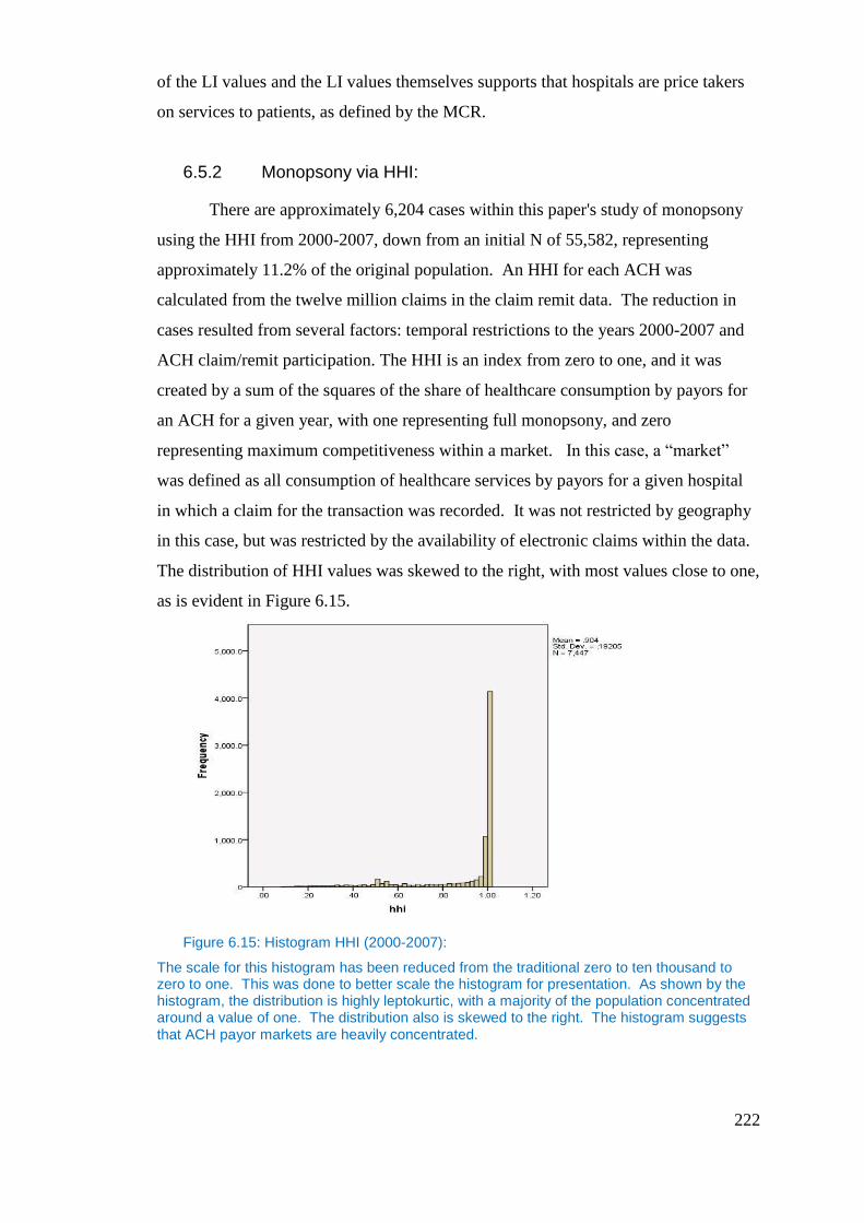
222
of the LI values and the LI values themselves supports that hospitals are price takers
on services to patients, as defined by the MCR.
6.5.2 Monopsony via HHI:
There are approximately 6,204 cases within this paper's study of monopsony
using the HHI from 2000-2007, down from an initial N of 55,582, representing
approximately 11.2% of the original population. An HHI for each ACH was
calculated from the twelve million claims in the claim remit data. The reduction in
cases resulted from several factors: temporal restrictions to the years 2000-2007 and
ACH claim/remit participation. The HHI is an index from zero to one, and it was
created by a sum of the squares of the share of healthcare consumption by payors for
an ACH for a given year, with one representing full monopsony, and zero
representing maximum competitiveness within a market. In this case, a “market”
was defined as all consumption of healthcare services by payors for a given hospital
in which a claim for the transaction was recorded. It was not restricted by geography
in this case, but was restricted by the availability of electronic claims within the data.
The distribution of HHI values was skewed to the right, with most values close to one,
as is evident in Figure 6.15.
Figure 6.15: Histogram HHI (2000-2007):
The scale for this histogram has been reduced from the traditional zero to ten thousand to zero to one. This was done to better scale the histogram for presentation. As shown by the histogram, the distribution is highly leptokurtic, with a majority of the population concentrated around a value of one. The distribution also is skewed to the right. The histogram suggests that ACH payor markets are heavily concentrated.

223
The resulting values close to one provided initial evidence of the high
concentration with which ACHs are confronted. The number of payors that ACHs
submit to electronically for reimbursement affected HHI values within the study. The
HHI or measure of market concentration was derived in this case by the amount of
healthcare consumed from a given hospital by payors. The ability to have an accurate
value for the HHI was determined by how many different payors and ACHs submitted
claims electronically. The lower the proportion of the number of payors submitting
electronically, the higher the likelihood that the HHI was skewed by not accounting
for all payors and services rendered. This may be the case, as some ACHs still submit
claims via paper.
In order to control for the payor count within the regression, a better
understanding of payor count is needed. In Figure 6.16, the box plot of the payor
count is very condensed and remains relatively compressed, with outliers present at
the upper end of the value range above 10 payors. The box plot is representative of
payor count values within the sample prior to the removal of outliers. The
distribution of payor count remained skewed to the left with high kurtosis. In Figure
6.17, a majority of the distribution of payor count values remained below a payor
count of 20.
Figure 6.16: Box Plot of Payor Count (2000-2007):
The box plot shows that the box and whiskers representing the normal distribution is being compressed by outliers within the sample.
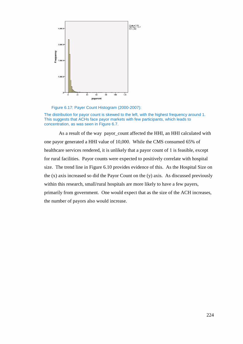
224
Figure 6.17: Payer Count Histogram (2000-2007):
The distribution for payor count is skewed to the left, with the highest frequency around 1. This suggests that ACHs face payor markets with few participants, which leads to concentration, as was seen in Figure 6.7.
As a result of the way payor_count affected the HHI, an HHI calculated with
one payor generated a HHI value of 10,000. While the CMS consumed 65% of
healthcare services rendered, it is unlikely that a payor count of 1 is feasible, except
for rural facilities. Payor counts were expected to positively correlate with hospital
size. The trend line in Figure 6.10 provides evidence of this. As the Hospital Size on
the (x) axis increased so did the Payor Count on the (y) axis. As discussed previously
within this research, small/rural hospitals are more likely to have a few payers,
primarily from government. One would expect that as the size of the ACH increases,
the number of payors also would increase.
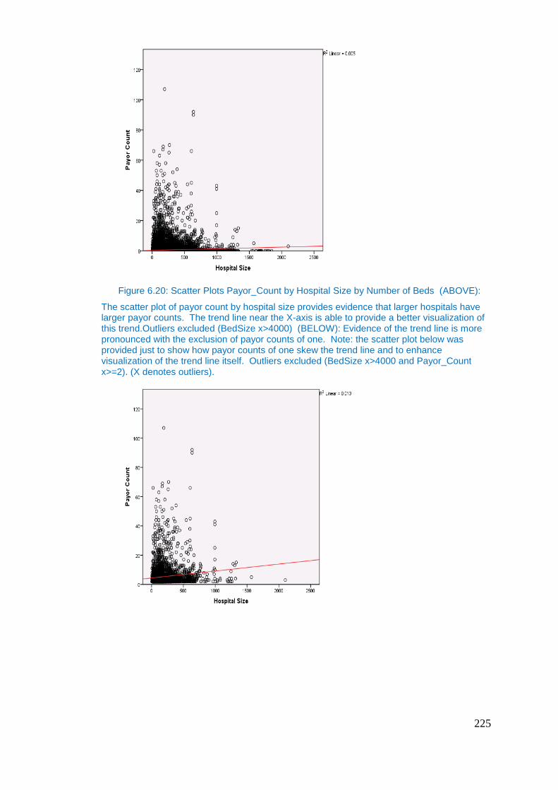
225
Figure 6.20: Scatter Plots Payor_Count by Hospital Size by Number of Beds (ABOVE):
The scatter plot of payor count by hospital size provides evidence that larger hospitals have larger payor counts. The trend line near the X-axis is able to provide a better visualization of this trend.Outliers excluded (BedSize x>4000) (BELOW): Evidence of the trend line is more pronounced with the exclusion of payor counts of one. Note: the scatter plot below was provided just to show how payor counts of one skew the trend line and to enhance visualization of the trend line itself. Outliers excluded (BedSize x>4000 and Payor_Count x>=2). (X denotes outliers).
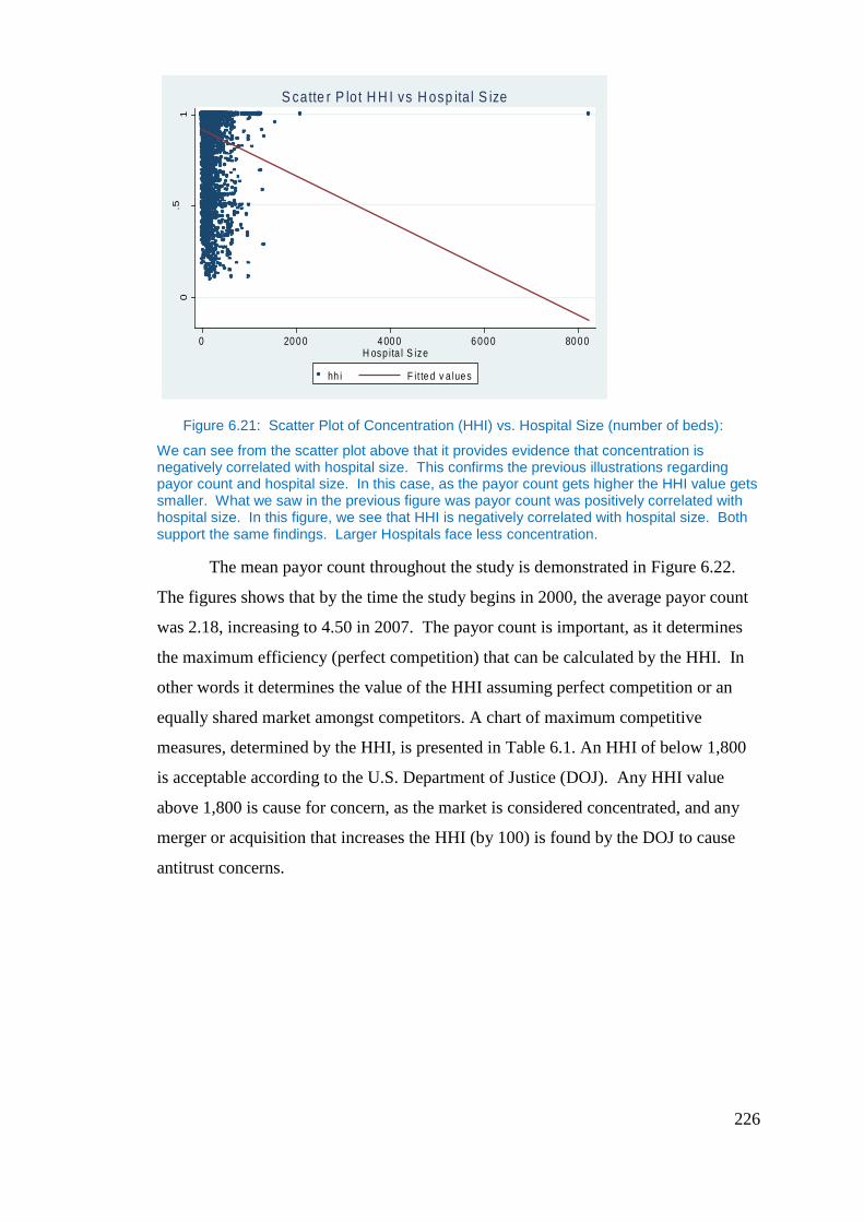
226
Figure 6.21: Scatter Plot of Concentration (HHI) vs. Hospital Size (number of beds):
We can see from the scatter plot above that it provides evidence that concentration is negatively correlated with hospital size. This confirms the previous illustrations regarding payor count and hospital size. In this case, as the payor count gets higher the HHI value gets smaller. What we saw in the previous figure was payor count was positively correlated with hospital size. In this figure, we see that HHI is negatively correlated with hospital size. Both support the same findings. Larger Hospitals face less concentration.
The mean payor count throughout the study is demonstrated in Figure 6.22.
The figures shows that by the time the study begins in 2000, the average payor count
was 2.18, increasing to 4.50 in 2007. The payor count is important, as it determines
the maximum efficiency (perfect competition) that can be calculated by the HHI. In
other words it determines the value of the HHI assuming perfect competition or an
equally shared market amongst competitors. A chart of maximum competitive
measures, determined by the HHI, is presented in Table 6.1. An HHI of below 1,800
is acceptable according to the U.S. Department of Justice (DOJ). Any HHI value
above 1,800 is cause for concern, as the market is considered concentrated, and any
merger or acquisition that increases the HHI (by 100) is found by the DOJ to cause
antitrust concerns.
0.5
1
0 20 0 0 4 00 0 6 0 0 0 80 0 0H osp ita l S ize
hh i F it te d v a lue s
S catte r P lo t H H I vs H osp ita l S ize
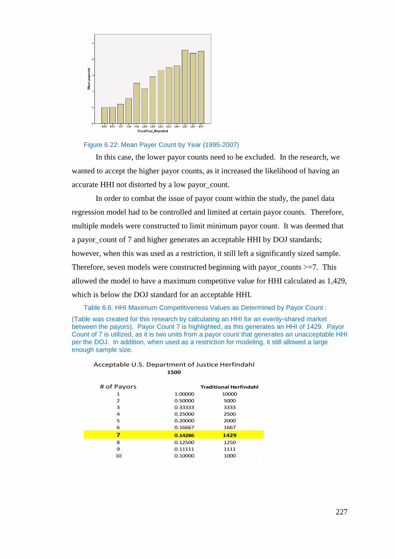
227
Figure 6.22: Mean Payer Count by Year (1995-2007)
In this case, the lower payor counts need to be excluded. In the research, we
wanted to accept the higher payor counts, as it increased the likelihood of having an
accurate HHI not distorted by a low payor_count.
In order to combat the issue of payor count within the study, the panel data
regression model had to be controlled and limited at certain payor counts. Therefore,
multiple models were constructed to limit minimum payor count. It was deemed that
a payor_count of 7 and higher generates an acceptable HHI by DOJ standards;
however, when this was used as a restriction, it still left a significantly sized sample.
Therefore, seven models were constructed beginning with payor_counts >=7. This
allowed the model to have a maximum competitive value for HHI calculated as 1,429,
which is below the DOJ standard for an acceptable HHI.
Table 6.6: HHI Maximum Competitiveness Values as Determined by Payor Count :
(Table was created for this research by calculating an HHI for an evenly-shared market between the payors). Payor Count 7 is highlighted, as this generates an HHI of 1429. Payor Count of 7 is utilized, as it is two units from a payor count that generates an unacceptable HHI per the DOJ. In addition, when used as a restriction for modeling, it still allowed a large enough sample size.
Acceptable U.S. Department of Justice Herfindahl1500
# of Payors Traditional Herfindahl
1 1.00000 10000
2 0.50000 5000
3 0.33333 3333
4 0.25000 2500
5 0.20000 2000
6 0.16667 1667
7 0.14286 1429
8 0.12500 1250
9 0.11111 1111
10 0.10000 1000
228
The correlation of number of payors and the traditional Herfindahl score can
be seen in Table 6.6. The calculated value assumed an equally-shared market
between all payors, thus creating the most competitive market, one with the lowest
possible HHI value for that number of payors. Acceptable DOJ values for the
Herfindahl were used in the study, as they present a marker for limits on other
markets in which the DOJ would interfere if concerns of monopoly were evident. To
qualify, monopoly is a form of inefficient market in which one supplier controls the
supply of a good for an entire market; it reflects the levels of market concentration of
supply. The buy side of the equation warrants the same concern as those on the supply
side, as they represent buyer market power and may cause consumer harm via
allocative inefficiency. Models then were constructed for payor_counts >=7, 6,
5…payor_counts>=1. The inclusion of all payor_counts allowed the maximum
sample to be utilized in the study.
The minimum mean HHI values, presented in Table 6.2, represent the smallest
HHI that could be calculated assuming equal pro-rata participation by all payors
within the research data for each year. While the minimum mean HHI values were of
concern when analyzed against the mean payor counts determined in the study, the
major concern was not the minimum mean HHI that could be calculated, but rather
the deviation of the actual mean HHI from that of the minimum mean HHI that could
be calculated. Table 6.2 shows the comparisons of the actual mean HHI with that of
the minimum mean HHI (most efficient). The deviation from the most efficient mean
HHI is quite extraordinary.
Even when the mean payor count moves to 4.56 in 2005, and an efficient
market HHI of 2,193 is possible, the actual mean HHI remains extremely high at
8,751. The evidence of market concentration is apparent in the difference in the
actual mean and the minimum mean possible. The high values of the HHI in Table
6.7, when compared against the acceptable DOJ standard of 1,800, verified that the
market is concentrated. In addition, the market is more highly concentrated than
would be available should all of the payors equally share the market equally. Given
the level of concentration on the buyers’ side of the market, as evidenced by the actual
mean HHI values, the question remains: Does such concentration of the buyer side of
the market have an effect upon the Real FCF?

229
Table 6.7: Efficient (minimum) HHI Possible to Actual Mean HHI by Fiscal Year Reported:
The mean payor count is the mean payor for each fiscal year of the study. The minimum mean HHI that has been calculated is the HHI value should the mean payor count have equal market share. This then is able to be compared with the actual mean HHI found within the study. The large deviation from the minimum mean provides evidence that the payor markets faced by ACHs are concentrated. The acceptable limit by the U.S. DOJ is an HHI value of 1,800.
All values above the minimum payor count for each model were allowed to
remain in the study. In theory, the large payor counts should generate lower HHI
values. Competition for acquiring service, in other words, increased demand for
healthcare products by payors, assuming a limited supply constrained at the number
of beds within a hospital should lead to increased prices, therefore more profit, and
greater FCFs for the ACHs. Similarly, if the level of competition for services
rendered is concentrated in the hands of a few payors, then more power would be
attributed to those consuming the services rendered. Concentration of buyer power
forces sellers to enter into transactions that are most likely less than optimum and are
inefficient. Under this condition, ACHs are more likely to have less profit and less
FCF, as was outlined previously.
By observing Figure 6.23, we can compare actual HHI versus the theoretical
competitive HHI values determined by the limitation of payor count on each model.
The theoretical competitive mean HHI was determined by taking the minimum payor
count allowed within the sample for each model and calculating an HHI based upon
equal sharing of the market. Therefore, in a market with seven payors, each payor
would have one-seventh of the market. If an HHI is calculated based upon this pro-
rata sharing of the market, we get an HHI value of 1,429. While higher payor count
values exist within the sample, by using the minimum, we set up the maximum
competitive HHI value achievable. The actual mean HHI was found to have a higher
value than that of the theoretical competitive HHI value for the same sample
limitations or payor count minimums. The difference between the actual and
Comparison Minimum HHI to Actual by Fiscal Year
Fiscal Year Mean Payor Count Minimum Mean HHI Actual Mean HHI
2000 2.18 4587 9434
2001 2.91 3436 9239
2002 3.33 3003 9148
2003 3.46 2890 9031
2004 3.59 2786 9050
2005 4.56 2193 8751
2006 4.37 2288 8458
2007 4.5 2222 8568
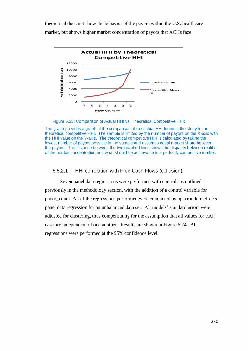
230
theoretical does not show the behavior of the payors within the U.S. healthcare
market, but shows higher market concentration of payors that ACHs face.
Figure 6.23: Comparison of Actual HHI vs. Theoretical Competitive HHI:
The graph provides a graph of the comparison of the actual HHI found in the study to the theoretical competitive HHI. The sample is limited by the number of payors on the X-axis with the HHI value on the Y-axis. The theoretical competitive HHI is calculated by taking the lowest number of payors possible in the sample and assumes equal market share between the payors. The distance between the two graphed lines shows the disparity between reality of the market concentration and what should be achievable in a perfectly competitive market.
6.5.2.1 HHI correlation with Free Cash Flows (collusion):
Seven panel data regressions were performed with controls as outlined
previously in the methodology section, with the addition of a control variable for
payor_count. All of the regressions performed were conducted using a random effects
panel data regression for an unbalanced data set. All models’ standard errors were
adjusted for clustering, thus compensating for the assumption that all values for each
case are independent of one another. Results are shown in Figure 6.24. All
regressions were performed at the 95% confidence level.
0
2000
4000
6000
8000
10000
12000
7 6 5 4 3 2 1
Herfi
ndah
l Hirs
chm
an In
dex
Payor Count >=
Actual HHI by Theoretical Competitive HHI
Actual Mean HHI
Competitive Mean HHI
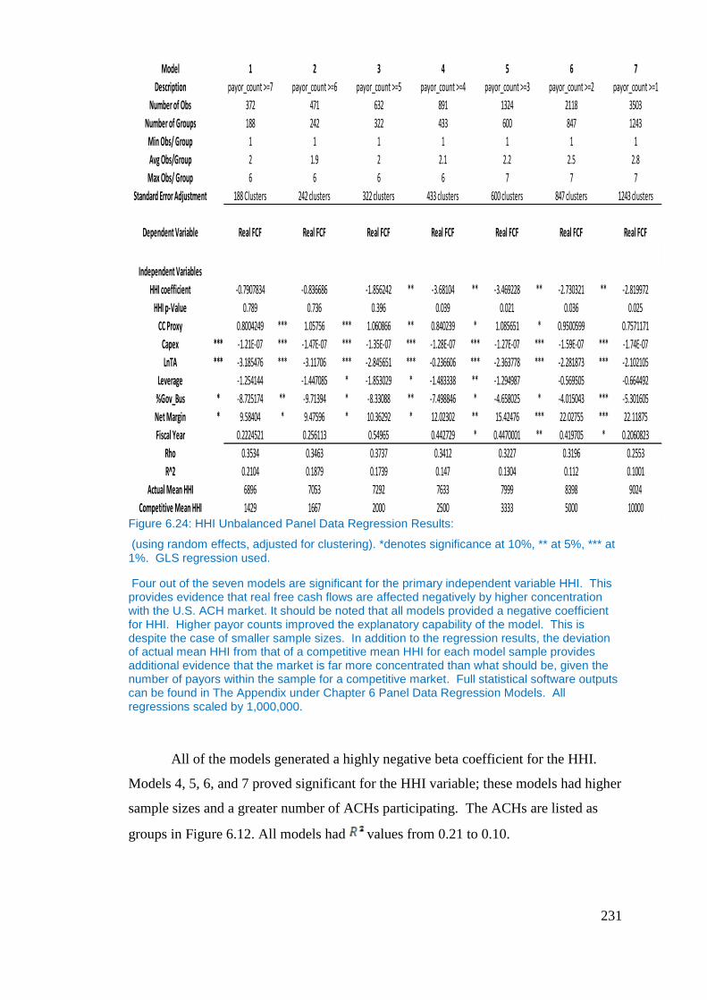
231
Figure 6.24: HHI Unbalanced Panel Data Regression Results:
(using random effects, adjusted for clustering). *denotes significance at 10%, ** at 5%, *** at 1%. GLS regression used.
Four out of the seven models are significant for the primary independent variable HHI. This provides evidence that real free cash flows are affected negatively by higher concentration with the U.S. ACH market. It should be noted that all models provided a negative coefficient for HHI. Higher payor counts improved the explanatory capability of the model. This is despite the case of smaller sample sizes. In addition to the regression results, the deviation of actual mean HHI from that of a competitive mean HHI for each model sample provides additional evidence that the market is far more concentrated than what should be, given the number of payors within the sample for a competitive market. Full statistical software outputs can be found in The Appendix under Chapter 6 Panel Data Regression Models. All regressions scaled by 1,000,000.
All of the models generated a highly negative beta coefficient for the HHI.
Models 4, 5, 6, and 7 proved significant for the HHI variable; these models had higher
sample sizes and a greater number of ACHs participating. The ACHs are listed as
groups in Figure 6.12. All models had values from 0.21 to 0.10.
Model 1 2 3 4 5 6 7
Description payor_count >=7 payor_count >=6 payor_count >=5 payor_count >=4 payor_count >=3 payor_count >=2 payor_count >=1
Number of Obs 372 471 632 891 1324 2118 3503
Number of Groups 188 242 322 433 600 847 1243
Min Obs/ Group 1 1 1 1 1 1 1
Avg Obs/Group 2 1.9 2 2.1 2.2 2.5 2.8
Max Obs/ Group 6 6 6 6 7 7 7
Standard Error Adjustment 188 Clusters 242 clusters 322 clusters 433 clusters 600 clusters 847 clusters 1243 clusters
Dependent Variable Real FCF Real FCF Real FCF Real FCF Real FCF Real FCF Real FCF
Independent Variables
HHI coefficient -0.7907834 -0.836686 -1.856242 ** -3.68104 ** -3.469228 ** -2.730321 ** -2.819972
HHI p-Value 0.789 0.736 0.396 0.039 0.021 0.036 0.025
CC Proxy 0.8004249 *** 1.05756 *** 1.060866 ** 0.840239 * 1.085651 * 0.9500599 0.7571171
Capex *** -1.21E-07 *** -1.47E-07 *** -1.35E-07 *** -1.28E-07 *** -1.27E-07 *** -1.59E-07 *** -1.74E-07
LnTA *** -3.185476 *** -3.11706 *** -2.845651 *** -0.236606 *** -2.363778 *** -2.281873 *** -2.102105
Leverage -1.254144 -1.447085 * -1.853029 * -1.483338 ** -1.294987 -0.569505 -0.664492
%Gov_Bus * -8.725174 ** -9.71394 * -8.33088 ** -7.498846 * -4.658025 * -4.015043 *** -5.301605
Net Margin * 9.58404 * 9.47596 * 10.36292 * 12.02302 ** 15.42476 *** 22.02755 *** 22.11875
Fiscal Year 0.2224521 0.256113 0.54965 0.442729 * 0.4470001 ** 0.419705 * 0.2060823
Rho 0.3534 0.3463 0.3737 0.3412 0.3227 0.3196 0.2553
R^2 0.2104 0.1879 0.1739 0.147 0.1304 0.112 0.1001
Actual Mean HHI 6896 7053 7292 7633 7999 8398 9024
Competitive Mean HHI 1429 1667 2000 2500 3333 5000 10000

232
Model 1 - which represented cases with payor counts >=7, and HHI was not
significant with a P-value of 0.789. The coefficient generated for HHI was -
0.7907834 Model 1 was constructed so that an efficient competitive market would
generate an HHI value below what the DOJ determined to be concentrated. Although
the coefficient was negative, the sample size was extremely small for a longitudinal
study, with only 372 observations and 188 hospitals participating for the duration of
over eight years. It was speculated that the small sample size prohibited the model
from being significant, as it was no longer representative of the population of ACHs
with a payor count greater than seven. On average, there were only 2 observations
per ACH, with a maximum number of observations of 6, and a minimum of 1.
Observing the HHI mean for the Model 1 sample showed that the actual mean HHI
was high, with a value of 6,896, in comparison to a competitive mean HHI of 1,429,
based upon the least payor count within the Model 1 sample.
Model 2 - represented cases with payor counts >= 6, and HHI was not significant
with a P-value of 0.736. The beta coefficient for the HHI variable was highly
negative with a value of -0.836686. Sample size remained small. There were 471
observations in total, with 242 participating ACHs. On average, there were 1.9
observations per ACH, with a maximum of 6 observations and a minimum of 1. The
HHI mean for Model 2 was 7,053, compared with a competitive HHI of 1,667, which
was based upon the minimum payor count within the sample for Model 2.
Model 3 - represented cases with payor counts >=5, and HHI was not significant,
with a P-value of 0.396. The beta coefficient for the HHI variable was highly
negative with a value of -1.856242. Sample size remained relatively small, with only
632 observations and 322 ACHs participating. On average, there were 2observations
per ACH, with a maximum of 6 and a minimum of 1. The actual mean HHI for
Model 3 was high, 7,292, in comparison to the competitive HHI value of 2,000. The
competitive value was the lowest HHI value that could be attained based upon the
minimum payor count within the sample.
Model 4 - represented cases with payor counts >=4, and HHI was significant for
with a P-value of 0.039. The beta coefficient for the variable HHI was highly
negative with a value of -3.68104. The sample size still was relatively small, with
831 observations; however, the number of ACHs participating had increased to 433
separate institutions. On average, there were 2 observations per ACH, with a
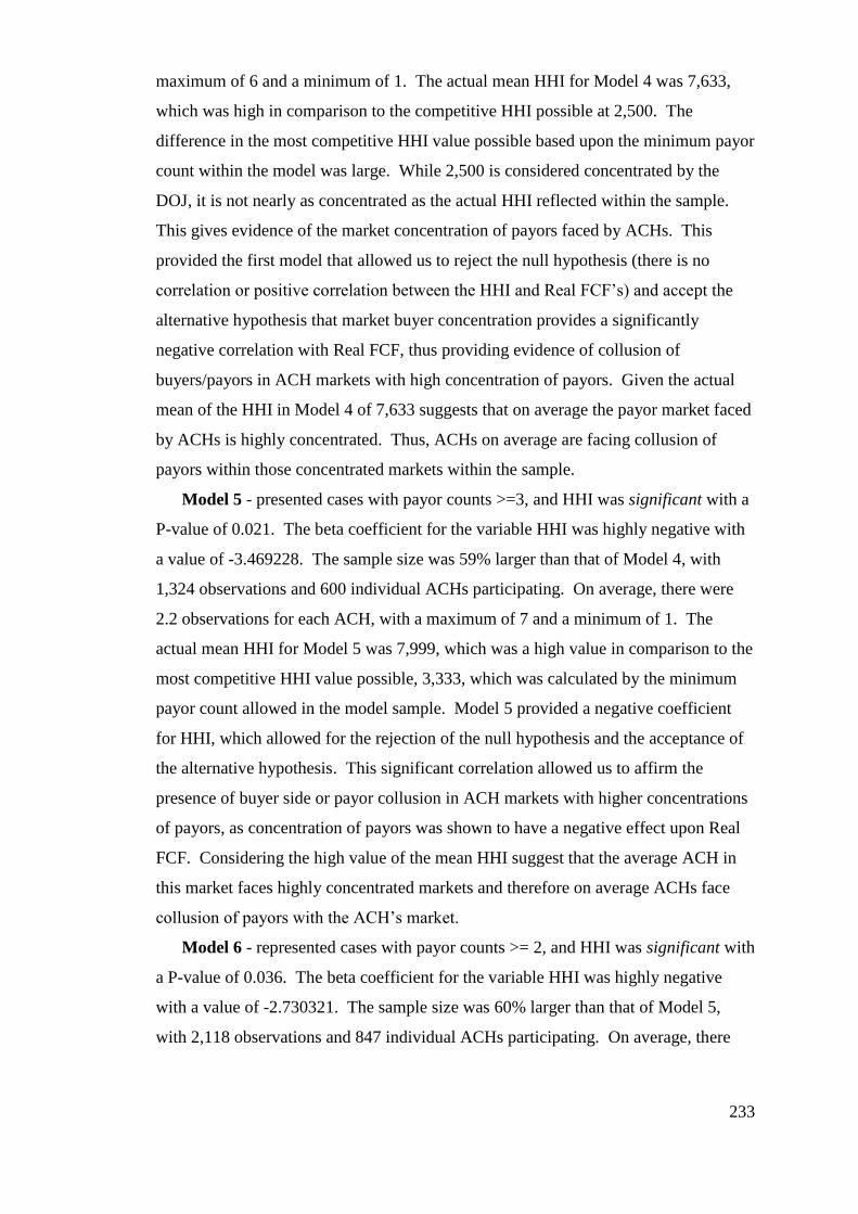
233
maximum of 6 and a minimum of 1. The actual mean HHI for Model 4 was 7,633,
which was high in comparison to the competitive HHI possible at 2,500. The
difference in the most competitive HHI value possible based upon the minimum payor
count within the model was large. While 2,500 is considered concentrated by the
DOJ, it is not nearly as concentrated as the actual HHI reflected within the sample.
This gives evidence of the market concentration of payors faced by ACHs. This
provided the first model that allowed us to reject the null hypothesis (there is no
correlation or positive correlation between the HHI and Real FCF’s) and accept the
alternative hypothesis that market buyer concentration provides a significantly
negative correlation with Real FCF, thus providing evidence of collusion of
buyers/payors in ACH markets with high concentration of payors. Given the actual
mean of the HHI in Model 4 of 7,633 suggests that on average the payor market faced
by ACHs is highly concentrated. Thus, ACHs on average are facing collusion of
payors within those concentrated markets within the sample.
Model 5 - presented cases with payor counts >=3, and HHI was significant with a
P-value of 0.021. The beta coefficient for the variable HHI was highly negative with
a value of -3.469228. The sample size was 59% larger than that of Model 4, with
1,324 observations and 600 individual ACHs participating. On average, there were
2.2 observations for each ACH, with a maximum of 7 and a minimum of 1. The
actual mean HHI for Model 5 was 7,999, which was a high value in comparison to the
most competitive HHI value possible, 3,333, which was calculated by the minimum
payor count allowed in the model sample. Model 5 provided a negative coefficient
for HHI, which allowed for the rejection of the null hypothesis and the acceptance of
the alternative hypothesis. This significant correlation allowed us to affirm the
presence of buyer side or payor collusion in ACH markets with higher concentrations
of payors, as concentration of payors was shown to have a negative effect upon Real
FCF. Considering the high value of the mean HHI suggest that the average ACH in
this market faces highly concentrated markets and therefore on average ACHs face
collusion of payors with the ACH’s market.
Model 6 - represented cases with payor counts >= 2, and HHI was significant with
a P-value of 0.036. The beta coefficient for the variable HHI was highly negative
with a value of -2.730321. The sample size was 60% larger than that of Model 5,
with 2,118 observations and 847 individual ACHs participating. On average, there

234
were 2.5 observations for each ACH, with a maximum of 7 and a minimum of 1. The
actual mean HHI for the sample of Model 6 was 8,398, with the mean competitive
HHI for the sample at 5,000. The difference between the two confirmed
concentration within the market by DOJ standards, as well as the deviation from the
most competitive HHI score possible based upon the minimum payor count within the
model. Model 6 also confirmed the alternative hypothesis and allowed us to reject the
null hypothesis. Concentration via high HHI values had a negative effect upon Real
FCFs; therefore, payor collusion is present in markets with higher payor
concentration. The high concentration represented by the mean HHI values in the
sample suggest on average ACHs in the sample face collusion of payors within the
ACHs market.
Model 7 - represented cases with payor counts >=1, and HHI was significant with
a P-value of 0.025. The beta coefficient for the variable HHI was highly negative
with a value of -2.819972. The sample size was 65% larger than that of Model 6,
with 3,503 observations representing 1,243 individual ACHs. On average, there were
2.8 observations per ACH participating, with a maximum of 7 and a minimum of 1.
The actual mean HHI for the sample was 9,024, with a competitive score of 10,000,
based upon the minimum payor count allowed in the sample of 1. Model 7 was
unique from the rest of the models created for the HHI in this research, as it was the
only one with a greater expected competitive HHI value than actually was found in
the sample in the model. The score of 9,024 provided evidence that the market was
more competitive than expected; however, it should be noted that 9,024 is still a
highly concentrated market. Of all the models created for this research, this model
provided the least evidence of collusion, even though it was significant.
6.5.2.2 Payor Concentration, Collusion, and NEIO:
The purpose of this section is to make use of the HHI and the findings of the
regressions within the section 6.5.2.1 along with the NEIO model to draw an
inference of the market power of payors within the healthcare market. This is
important, as no data is available to measure market power directly by calculating
Lerner’s index for payors within this research. The NEIO provides a methodology,
which allows the research to examine, and infer the market power of the payors by
inferring values of the payors Lerner’s Index. This allows the model to consider not

235
only market power of the ACHs (the consumer) via the previously calculated Lerner’s
Index for ACH’s, but also allows the research to exam market power for the other
market participant on the demand side of the transactions the payors.
While market concentration does not directly correlate with market power, we
know that cooperative pricing, as suggested via collusive monopsony, is more likely
in a concentrated market (Cabral, 2000). In addition, payors within the market are
competing with one another for inputs of healthcare services to deliver to their
insured. Payors [insurance companies] only can affect demand by their insured for
health services slightly via co-pays and deductibles. As payors do not compete for
inputs (health services) and cannot readily control demand for inputs (health services),
it is more likely that they will try to reduce the amount paid for inputs (health
services) to its minimum.
Ordinarily, in a competitive market with many payors, there would be
competition for inputs from ACHs. The demand for inputs of health services would
lead many payors to increase the prices paid to a more competitive price for the
inputs. In a concentrated market this is not so, as the competition for inputs is less.
Now, consider the opposite side of the equation for payors (health insurance
companies), in which they compete in a competitive market to supply financing of
healthcare services. Their product (healthcare financing) is the combination of price
and quality/breadth of coverage provided. In the market for healthcare financing
(health insurance), price is elastic to demand; therefore, the pricing of their product
(health insurance) has influence on demand and therefore revenues. If prices are
lowered to compete with other insurers, some revenues are forgone from the current
customer base in order to obtain new customers from competing firms. If payors are
to maintain margins, they must reduce their costs of coverage. Their largest expense
is the health services that they finance via insurance premiums. The lower they obtain
these inputs (health services), the better their margins, or the better they can compete
in the competitive market. Payors have tremendous incentive to obtain inputs at the
lowest possible price. Given the payor’s ability to obtain pricing information from the
price leader, Medicare and Medicaid, via public information, payors are able to utilize
this information to press ACHs into pricing for health service inputs parallel to those
of Medicare and Medicaid. In addition, one must consider that contracts are
negotiated with ACHs once a year, which gives payors additional strength in
236
negotiations, due to the renewals and length of contractual time periods. Given the all-
or-nothing contractual nature of payors with ACHs, this pricing does not take place on
the marginal cost curve, but rather on the average cost curve, as suggested by Taylor
(2003).
6.5.2.3 The New Empirical Industrial Organization (NEIO):
It has been suggested when using the NEIO21
that market power measured by
the LI is comprised of three main variables that determine market power:
concentration of the market, collusive behavior, and price elasticity of demand
(Cabral 2000). The relationship is expressed in Equation 6-8.
In order to show that payor concentration within the market for healthcare
services equates to collusion and market power, one must consider two variables that
have not been calculated yet within the research: price elasticity of demand and
collusive behavior. Evidence provided by previous research suggests that the moral
hazard of insurance is strong within the market for healthcare services and that
competition for patients is driven by quality of health services, not the price of
healthcare services, as patients are not exposed to price due to health insurance
(Nahata 2005). Given this characteristic of the market, one must assume that demand
for ACH services by patients is strongly inelastic to the price. Any change in price is
less likely to cause a large percentage change in demand by patients. Therefore, we
21 NEIO or The New Empirical Industrial Organization is an empirical methodology, which seeks
to use systematic statistical evidence in the effort to study single industries as opposed to a cross
section of industries, utilizing the relationship between demand elasticity, market concentration (as
measured by the Herfindahl Hirschman Index) and collusive behavior and market power (as measured
by the Lerner’s Index), (Cabral 2000). The main principles behind the use of the NEIO model is that
price cost margins cannot be observed, therefore an inference can be made from the behavior of
industry firms to identify changes in marginal cost (Waldman and Jensen, 1998). The primary focus of
the NEIO and most research that utilize this methodology is its use to measure the market power of
firms. The NEIO has been especially helpful to researchers seeking to find evidence of collusive
behavior and in research, which focuses on analysis of market structure, firm conduct and market
performance in oligopolistic markets (Martin 1994; Walden and Jensen 1998 and Cabral 2000). The
NEIO is meant to be an improvement on the Structure-Conduct-Performance model or SCP.

237
assume elasticity of demand for the industry as a constant value within the course of
this research. In addition to this, an assumption can be made for the value of elasticity
of demand: that it is most likely close to zero (a zero value denotes complete price
inelasticity).
The equation for market power (NEIO) shows that a constant value for the
elasticity of demand implies a positive correlation between the HHI and the LI. This
leaves the calculation of market power (Lerner’s Index) reliant on the presence of
collusive behavior within the market. If there is collusion, then there is market power,
and if no collusion is present, then no market power is present.
Equation 6-8: New Empirical Industrial Organization (NEIO)
L- Lerner’s Index (measuring market power of the Payors)
H- Herfindahl Hirschman Index (measures market concentration of the Payors)
Θ- Collusive Behavior (measures market collusion of Payors)
ε – Demand Elasticity (measure percentage change in quantity demanded per 1%
change in price)
We now explain why we believe that in Equation 6-8 that Θ has a value
indicating collusion in this industry. If the high concentration measured by the HHI
has a negative effect upon real free cash flows of ACHs, then collusion between
insurers is likely to exists. It is known from the regression analysis that payor HHI
values are correlated negatively with real free cash flows of ACHs. Therefore, a high
HHI in the payor market results in low real free cash of the ACH. Hence, collusion
must be present within the market. If there were no collusion by payors, then a more
concentrated market would not have a negative effect upon the real free cash flows of
ACHs.
The ACH market has shown a high concentration of payors within the market.
This is reflected in the high actual HHI values calculated in this research. In addition,
empirical evidence has shown that a high HHI has a negative effect upon free cash
flows of ACHs, resulting in the conclusion that this is the effect of the collusion of
payors.

238
Given the assumption of high inelasticity of demand within the market for
healthcare services, the presence of highly concentrated payor markets with clear
evidence of collusion reflects that payors within the ACH market wield market power.
Market power is manifesting itself in the empirical evidence via high HHI values
(measuring concentration) and the negative correlation of free cash flows (measuring
collusion) associated with the HHI. The evidence provided by the regression analysis
suggests two conditions exist within this U.S. ACH market: 1) There is collusion
present among the payors of the U.S. healthcare system in concentrated markets; and
2) There is high market power of insurers in markets with high concentration. If there
is no market power, there is no collusion. If there is no collusion, how is it that ACH
real free cash flows suffer when there is an increase in the payor concentration?
6.5.2.4 Payor Market Power and Cournot Equilibrium:
If one considers this market in light of the Cournot equilibrium, in which all
payors choose how many healthcare services to consume at the same time, Θ22
in the
NEIO model would be valued at one (no collusion). This would allow for a high LI
as well, and explain the correlation between the HHI and LI. The dilemma with this
inquiry is that in this case, payors do not choose the amount of healthcare services
consumed, rather, the individual patients covered by health insurance do. Therefore, a
Cournot equilibrium is not possible, as payors cannot choose consumption rates or
rather the output of healthcare insurance dollars. Therefore, Θ must represent either
collusion (1/H) or a value close to zero.
Assuming collusive behavior and the high inelasticity of demand in Equation
6-8, if the HHI is increased, the LI increases. Therefore, if there is a high HHI, then
one can equate the high value of the HHI in this case into a high LI. The high LI for
22 Definitions for the Possible Values of Theta:
1 = Cournot Equilibrium
0 = Bertrand Competition
1/H=Perfect Collusion
239
payors represents the market power of the payor, which in this case represents
collusive monopsony amongst payors.
The environment, which consists of payor market power, is one that is creating
inefficiencies within the market for ACHs. This inefficiency of payor market power
is having a negative effect on ACHs’ free cash flow, and is affecting capital structure
decisions accordingly. The lower the free cash flows, the greater the limitation ACHs
have accessing debt markets, and the higher the opportunity cost becomes for the uses
of those cash flows. We know that ACHs must compete on quality, as price greatly is
removed from the equation due to moral hazard; consequently, patients are choosing
ACHs upon perceived quality of care. This great reliance on the perceived quality of
care causes hospitals to invest in capital items that allow for increases in perceived
quality (Nahata 2005). As discussed in Chapter 4, the limitations placed on access to
capital and possibly an increased cost of capital hinder the organization’s growth, as
well as cause ACHs’ management to have higher requirements for the investment of
the capital that is available. Therefore, monopsony restricts choices of capital
structure, making ACHs more dependent on internal funds.
6.6 Conclusion
The primary goal of the research within this chapter was to provide evidence
of collusive monopsony and examine its effect upon decisions of capital structure.
This is important, as it has been proposed in previous research that the government
allows a collusive monopsony to exist in order to control the costs associated with
overinvestment. It also has been suggested that low prices compensating ACHs for
healthcare services resulted from a function of collusive monopsony impacting FCFs,
which consequently affected decisions of capital structure, as limiting FCF restricts
access to debt markets and causes ACHs to be more dependent on internal funds.
While the previously discussed literature of Pauly (1998), Sevilla (2005), and
Seth (2006) has suggested the presence of monopsony within the healthcare market,
others, such as Feldman and Wholey (2001), have suggested that conditions within
the healthcare market were not an effect of monopsony, but rather of monopoly-
busting behavior. For the research to proceed, it was prudent to provide evidence of
two phenomena: 1) the existence of collusive monopsony and the resulting negatively
240
impacted free cash flows of ACHs; and 2) ACHs do not possess market power and are
price takers within the market.
Evidence of monopsony was provided via a three-step process. An HHI value
was calculated for each ACH for each year of the study from claim and remittance
data. This provided a basis to measure market concentration of the payors within the
ACH market. The values calculated then were compared with values of the HHI
considered by the U.S. DOJ to be representative of a concentrated market.
Concentration was confirmed, as the lowest actual mean HHI of 8,458 compared with
the DOJ limit of 1,800 is proof of concentration of the market; however, more
remarkable was the actual mean HHI comparison to a value of HHI for equally shared
market of 2,288 for the same year.
Evidence of collusion of payors was provided by the panel data regression on
the Real FCFs, which shows the negative effects that concentration has upon Real
FCFs. The beta for the HHI was highly negative, and the P-value was significant in
Models 4-7. While Models 1, 2, and 3 were not significant, this can be construed as
the result of the small sample skewing the results. In all cases, the beta for the HHI
was highly negative, indicating that the HHI has a negative relationship to the Real
FCF. For every 1-unit increase in the HHI, Real FCFs were reduced by a range of
$2,730,321 to $3,681,040. Cabral (2000), suggested that collusion is more likely to
occur in markets with greater concentration.
The NEIO supports collusive monopsony by combining the concentration and
collusion of the payor market faced by ACHs. The NEIO provided a model with
which to examine the relationship of payor concentration, collusion, and demand
elasticity with market power. In this case, payor market power is interpreted as
collusive monopsony. An assumption was provided in the research for demand
elasticity of health services consumed by payors, which allowed the NEIO to support
market power by payors. The effect of concentrated payor markets on Real FCF was
shown to be collusion, as a Cournot equilibrium was ruled out.
The lack of monopoly power by ACHs was supported by the calculation of an
LI using payment information provided via the claims data. The LI is a measurement
of market power that analyzes the excess return captured by firms. Using nine health
procedures that are technologically stable throughout the longitudinal study, akin to
Sevilla (2005), LIs were calculated for each procedure. Then, all of the LIs were

241
averaged for each ACH each year. The LIs supported the lack of monopoly power by
ACHs, as all mean LI values presented were negative for each year of the study. Each
LI then was regressed upon the NISP to confirm price taker status. The regression
provided a positive correlation of the LI and NISP, suggesting that market power or
the lack thereof affects revenues derived from insurers. As each LI provided low
values, this suggested that the lack of market power by ACHs meant the lack of
market power was reflected in lower revenues derived from insurers, which supports
the price-taking status of ACHs.
The research provided evidence of collusion of payors equating to market
power of the payor, or monopsony. In addition, it showed that ACHs lack market
power and are price takers. Therefore, the research supported the previous findings of
Pauly (1998), Sevilla (2005), and Seth (2006), all of whom suggested that monopsony
has effects within the healthcare market. Likewise, the research was able to utilize
ACH price-taking status to confirm evidence of impact resulting from the all-or-
nothing contractual arrangement with ACHs. There is clear evidence of collusive
monopsony by payors in the ACH market. Collusive monopsony has a negative
impact on Real FCFs, restraining access to debt markets and increasing borrowing
costs. The restriction in access to debt markets limits choices of capital structure by
managers of ACHs; thus, ACHs are more reliant upon internal funds for investment.
Higher borrowing costs force managers to limit the use of debt. Reliance upon
limited internal funds for investment increases opportunity costs of investments, and
thus increases the requirements for performance of investments.
The increase in requirements for the performance of investments means
managers of ACHs are less likely to invest in questionable projects or projects that
might be viewed as over investment by the government. Thus, the government is able
to control overinvestment by allowing collusive monopsony to exist within the
market. This reduction in overinvestment lowers the costs of providing healthcare to
citizens covered by government programs, as costs associated with low return projects
usually were supported by increased costs to insurers, including Medicare and
Medicaid. Collusive monopsony is an effective tool in controlling ACH behavior.
Capital structure decisions are affected, as a reduction in FCFs limits access to
debt markets and leaves ACHs reliant upon internal cash flows in order to finance
projects. Given that ACHs compete on quality and must make heavy capital
242
investment in order to remain competitive, this restricts ACHs in their investment
opportunities, and as a result, they may be harmed fiscally by an inability to compete.
Because low FCFs limit access to debt markets, any debt taken on by the ACH
in such a condition may be burdened by the higher capital cost associated with such
debt. In all cases, whether totally reliant on internal funds or borrowing in restrained
debt markets, the ACH’s management is impacted negatively by the presence of
monopsony within the ACH healthcare markets. While some may view the presence
of monopsony within the market as a necessary construct to keep costs down, it is
unlikely that the true understanding of the impact on ACHs is being realized. It is in
the long run that the greatest harm due to exposure to monopsony is realized
(Bradfield 1990)
6.7 Contributions to Knowledge
These findings contradict the findings of Feldman and Wholey (2001), who
concluded that lower prices for healthcare services were emblematic of a breakup of
the ACHs’ monopoly power. The ACHs are impacted by collusive monopsony, and
combined with the lack of market power of ACHs, this means that ACHs’ decisions
of capital structure are affected heavily by the construct in the healthcare market.
This research concluded, similarly to Pauly (1998), Sevilla (2005), and Seth (2006)
that healthcare is affected by monopsony power. Although Sevilla (2005) analyzed
the laboratory market for services, the payment mechanisms are similar to the ACH
market, and similar behavior is found in both. While Pauly (1998) suggested that the
quantities of inputs consumed under lower prices would determine the possible
presence of monopsony, the present research added the consideration of the all-or-
nothing contractual arrangements, analogous to Sevilla (2005), under which many
ACH services are provided. This research showed evidence of monopsony power
using the NEIO framework. The research also considered both the market power of
the payor and the ACH within the same framework. A clearer understanding of
pricing and payor concentration by ACH was provided by a combination of the MCR
and claims data provided by the private sector. This combination of methodologies
and data was not used by previous research.
243
7. Thesis Summary and Conclusion
The goal of this research was to provide evidence of market distortions via
agency and collusive monopsony and examine the effect of such distortions on
decisions of capital structure of ACHs within the U.S. The MCR and a unique
proprietary database of electronic healthcare billings and remittances from 2000-2007,
allowed for the examination of the U.S. healthcare market and ACHs for these
distortions. The ACH financial data was examined for evidence of agency cost via
signaling and agency cost of free cash flows. Both were proposed to exist because of
the underlying principal-agent relationship created by the inability to form a complete
contract between the federal government and ACHs. This was suggested because the
U.S. Government covers or provides insurance for citizens via several government
programs, namely Medicare and Medicaid.
7.1 Agency Costs
Competition within the ACH market is driven by quality or the perception of
quality due to the moral hazard of insurance for patients. Previous research has
shown that competition on quality leads to overinvestment by ACHs in cutting-edge
technologies and services as well as facilities (Newhouse, 1981; Glied, 2003; Nahata,
2005). The excess cost of healthcare derived from overinvestment is of concern to
government, as it consumed 65% of health services delivered during the term of this
study (1995-2007). The government, concerned with overinvestment, seeks to control
free cash flows of ACHs, thereby limiting the overinvestment behavior and reducing
agency costs. Because the government does not provide healthcare services directly,
and must contract for these services, this research theorized that agency cost exists
and affects acute care hospitals financially. This is similar in structure to the way that
agency affects the traditional firms, as was proposed by Jensen and Meckling (1976)
and Jensen (1986), with an expansion of the principal agency relationship akin to
Milgram and Roberts (1992) and Ross (1973).
Two linear regression models were created to seek the existence of both
phenomena of the agency relationship. Signaling was tested via the regression of
debt on the percentage of government business, using an alternative hypothesis of
positive correlation of debt and government business. The model was designed to

244
show whether ACHs signaled efficiency via debt in order to obtain greater
government business. The ACHs signaled efficiency with the use of debt, thus
incorporating third-party monitoring, which reduces agency cost.
Agency cost of free cash flows was tested via a linear regression of the
percentage of government business on free cash flows of ACHs using an alternative
hypothesis: the higher the percentage of government, the lower the free cash flows.
While no evidence of signaling was found, there was significant evidence of agency
cost of free cash flows. For a one percent change in government business, free cash
flows of ACHs were reduced by a range of $953,518.00 to $1,166,087.00. The
presence of agency cost of free cash flows helps explain the lack of signaling present
within the market, as the reduction in free cash flows restricts access to debt markets,
thereby limiting ACHs’ ability to signal. In addition, the restriction in debt markets
limited via agency cost of free cash flow limits decisions of capital structure by
ACHs, as they are dependent upon internal funds for access to debt markets (Calem &
Rizzo 1995). As ACHs are more dependent on internal funds due to lower free cash
flows, the opportunity cost of investment increases, changing the performance
requirements for future projects and thereby reducing overinvestment.
7.2 Collusive Monopsony
Previous research by Pauly (1998), Sevilla (2005), and Seth (2006) suggested
that monopsony was or could be present in the U.S. healthcare market. The research
hypothesized a collusive monopsony to exist within the U.S. healthcare market, as the
U.S. Government via Medicare and Medicaid consumed, on average, 65% of health
services during the years of 1995-2007. In addition, the fee schedule and policies of
Medicare and Medicaid are made public, allowing other payors to obtain this
information. It was proposed that the use of this information by other payors allowed
them to change the prices paid for procedures in correlation with Medicare and
Medicaid, thus creating collusion and market power by allowing them to internalize
additional market rents above the competitive norm. Similar to Seth (2006), in order
to capture the concentration of the payor market relative to each ACH individually,
using unique claims data, an HHI was created for the payor market faced by each
ACH. This effectively measured the concentration of payors in each geographic
245
healthcare market. In addition, using the unique claims/remittance data for nine
patient procedures, a modified LI using average total cost was calculated for each
hospital, thereby allowing an examination of market power and price taker status of
the ACHs.
In order to provide evidence of collusion within the market, a regression was
conducted using panel data regression of the concentration of the payor (HHI) on the
real free cash flows of the hospital. This provided significant evidence of collusion, as
the concentration of payors was shown to have negative effects upon ACHs’ real free
cash flows. For every increase of one in the value of the HHI, real free cash flows
decreased, ranging from $2,730,321 to $3,681,040. This suggested that collusion
manifests in markets with higher payor concentration, as was expected (Cabral 2000;
Lipczynski et al 2009). An additional inference of the market power of payors was
made, as prior research had shown a high inelasticity of demand within the market
due to the moral hazard, which insulated patients from price (Maynard 2001; Gaynor
et al. 1999; Glied 2003; and Pauly 2004). While ruling out Cournot equilibrium, the
research was able to show via the New Empirical Industrial Organization NEIO
model that high concentration and collusion equates to market power of payors; thus,
a collusive monopsony is present in the U.S. ACH market.
The numerical value of the modified LI provided evidence of a lack of market
power, as the average modified LI for each year was negative. The low value of the LI
confirmed that ACHs have negative margins on the procedures rendered to patients of
payors. This suggested that ACHs have little market power. In order to provide
additional evidence of this, two models for the LI were proposed. First, a regression
of the LI on real free cash flows of the ACH that used panel data regression to
understand better the lack of market power of hospitals effect on decisions of capital
structure via free cash flows. The second, a regression of the LI on the NISP, which
provided support of ACHs as price takers. The use of both models provided an
alternative viewpoint to the results of the HHI.
The LI regression provided evidence that suggested that the FCFs were not
affected by the lack of market power of ACHs. The results did not match expected
outcomes as components within free cash flows were thought to be distorting the
effects of the lack of market power of ACHs. Namely revenues derived from other
income as defined by the MCR was thought to be skewing results as they are counter
246
balancing negative margins received by ACHs on services rendered to patients. This
intellection is supported by the evidence comparing the net income margin and
operating margin for ACHs. Net income margin, which comprised both Net Income
from Service to Patients and Other Income, was positive, while Operating Margins,
which comprised only revenues from services to patients, was negative during this
longitudinal study. Therefore, a further regression of the LI on the NISP was
conducted to show that market power as measured by the LI did significantly support
price taking within the ACH market for the NISP. This provided better results, as the
net income from patient services is income primarily received from insurers, and
therefore delivered a better indication of price taking. The result of the HHI and the LI
regressions supports the existence of collusive monopsony and the price-taker status
of the ACHs. In addition, collusive monopsony had a large negative influence on free
cash flows. Thus, collusive monopsony had negative consequences for decisions of
capital structure by reducing or limiting free cash flows.
7.3 Implications
The implications of these results require us to consider how the research may
effect, agency research, monopsony research , constructs in market that cause
distortional effects upon market participants and future research directions.
7.3.1 Agency Research
The research presented here has implications for future agency research. This
contends that agency costs are present in a principal-agent relationship which is not
considered amongst the traditional agency relationships. As such, this research
considers the agency problem more in line with Milgrom and Roberts (1992) and
therefore views agency relationships as more widespread in society than perhaps that
considered in the mainstream finance literature or as expressed by Jensen and
Meckling (1976). The presence of agency costs of free cash flows suggests that
researchers should look at markets and relationships where agency might not be
thought to exist and to realize that the implications of these agency costs could be
more detrimental to non-parties to the agency relationship, in this case patients.

247
7.3.2 Monopsony Research
The implications for monopsony research are not quite as obvious as those for
agency theory. The research presented evidence of collusive monopsony as proposed
by Taylor (2003) under the all or nothing contract. This presents a slight deviation
from the traditional monopsony approach, and the one in which the previous literature
had sought, unsuccessfully, for evidence of monopsony in healthcare, due to the
approach of examining the market for a reduction in consumption along with price.
This research, on the other hand, suggests that monopsony may in fact be present in
markets where previous empirical studies had suggested there was none, leaving one
to consider the validity or need to readdress current views as exppressed in prior
research on this topic. The contractual arrangements inherent within a market can
change how market power should be analysed and how a researcher might seek
evidence thereof. Likewise this research undertaken in this thesis may suggest that
more consideration be given to the detrimental effects of monopsony when regulating
a market for antitrust behaviour and policy determination. The findings presented
here suggests that monopsony’s presence while initially apparently a good outcome
for the payor and a benefit for the end consumer, ultimately may not be in the long
run as the distortions created by its presence take time to manifest.
7.3.3 Research Structure and Methodologies
The research presented novel ways of seeking evidence of both agency and
monopsony. Both the methodologies used were structured to analyse the data and
seek evidence of the primary theory along with an alternative, namley a mirror image
phenomena which would give negative results. In the case of the research on agency,
both a theory of signalling and agency cost of free cash flows were considered. No
evidence of signalling was found and yet evidence was found for the agency cost of
free cash flows. Combined these results provide evidence that a reduction in free cash
flows was effected by agency. It should come as no surprise that lower free cash
flows would reduce the ability of ACHs to signal via debt. So a lack of evidence of
one condition helps to support the evidence that another condition was present.
Likewise, when seeking evidence of monopsony, market power for both sides of
the market was considered (buyer and seller). This allowed the research to provide
248
evidence that collusive monopsony was present for buyers (payors) but lacking for
sellers (ACHs). This dual approach allowed the findings of a lack of market power on
the part of ACHs to support the findings that the payors have collusive monopsony
power. This is important as these twin approaches to the research may provide an
alternative method for finance and econometric research going forward to address
similar questions as to those covered in this thesis. In addition, the combination and
use of the Lerner’s Index, Herfindahl-Hirschman Index and the NEIO model in a
combined approach presents a possible consideration to move forward monopsony
research, especially in the area of healthcare. Finally, suitably adapted, the combined
approach used here might have implications for other areas of research in economics
and finance.
7.3.4 Market Implications
While agency cost of free cash flows was found to affect free cash flows of
ACHs, the influence of monopsony on real free cash flows of ACHs is much more
profound. In either case, managers of ACHs are placed under constraints in managing
capital structure, as free cash flows are limited by both distortions in the market. 23
The ACHs’ access to debt markets is limited, as they must promise future free cash
flows in order to obtain debt. Without access to or constraints on debt, ACHs find
themselves squeezed as they compete in a market that requires large capital
23 While some may suggest that reductions in free cash flows do not constrain decisions of capital
structure, let us consider if a reduction in free cash flows actually constrains the ability to obtain debt.
Lending institutions have lending limits, which usually encompass covenants, which require firms to
stay within a given ratio during the term of the financing. Likewise, firms falling below given financial
ratio requirements will not be able to raise debt. Further, let us consider moreover that lenders have a
maximum multiple of free cash flows they are willing to lend, for example a coverage ratio. Now let
us assume that hospitals always borrow at the maximum allowed by the lender. If the ACH
experiences a reduction in free cash flow then the lending limits allowed by the lender will be reduced
by the multiple of the reduction in free cash flows multiplied by the lenders maximum lending ratio.
This therefore limits the amount of debt that a lender is willing to consider providing to ACHs. This
reduction in debt capacity places a constraint on capital structure as it reduces that ability of ACHs to
take on additional projects, which would cause the ACH to exceed its debt capacity.

249
investments. In addition, moral hazard within the market insulates their consumers
from payment, so that ACHs compete more readily on quality or perceived quality
(Newhouse 1981; Nahata 2005). Therefore, if ACHs cannot take on projects that
enhance perceived quality, their competitiveness within the market is hindered. The
possibility of ACHs being marginalized financially in the presence of agency and
monopsony is possible, thus pushing already troubled ACHs into the margin or into
insolvency.
These findings are troubling for an industry that already is having financial
difficulties. Management of the ACHs in this current environment is challenging at
best, and at worst, impossible. The real concerns of these distortions, especially
monopsony, are that it is not the short-run effects that harm the industry, but rather the
long-run consequences 24
(Bradfield 1990). The ACHs deliver healthcare in a very
difficult market in which consumers seek the most advanced healthcare provider
covered by their insurance. Moving forward, because of the lack of free cash flows
and consequently limited or lacking access to debt markets, ACHs may choose not to
invest in additional capital projects, but to maximize utilization on older technologies.
While at first this may seem to be an excellent management choice for a firm’s
survival, given the healthcare market and the moral hazard, the quality of services will
ultimately suffer, as ACHs cannot afford to modernize, therefore perhaps leaving
better treatments for ACHs with better cash flows. This alludes to a reduction in
24 The long run consequences presented by both agency costs of free cash flows and collusive
monopsony are that cash flows of ACHs are negatively impacted. Mean net margins for ACHs over
the study range from 1% to 3%. Any slight decrease in free cash flows affects the ability of ACHs to
invest in future capital projects and/or services, as it limits both investment via internal funds, but also
reduces access to debt as ACHs have less cash flow to promise for debt repayment. As reimbursement
increases have not kept up with inflation in healthcare costs, this leads to an erosive effect in on two
fronts. One that free cash flows are reduced by increasing business with the federal government and/or
through negotiations with payors via collusive monopsony. This may lead to a scenario where margins
are squeezed as ACHs can only cut so much cost and efficiency before they affect quality of care. Two
is that if reimbursement scheme are kept low and increases do not match inflation then ACHs will be
losing revenues in real dollar terms. Neither of these facts immediately present themselves as a
problem in the short term, but rather in the long term become detrimental to ACHs financial wellbeing.
250
quality or breadth of healthcare services provided, which brings light to the concern
over long-term consumer harm. This is cause for concern as antitrust legislation, as it
is currently enforced, ignores consequences to consumer harm via indirect means.
Previous research has recognized the gaps between small, rural hospitals and large,
urban medical centers; these gaps only will widen under this scenario, making equal
access to healthcare difficult. The continuation of these market distortions is not
healthy for the ACH market or for the patients. This research may suggest that better
methods for controlling cost may need to be found as price paid by the payors has
little control over healthcare cost. Perhaps a more relevant strategy would be to
increase cost sharing by patients, thereby leaving a margin on which ACHs may
depend to remain valid providers of quality healthcare and relying on greater control
of consumption by the end consumer.
7.3.5 Policy Implications
The findings of this research presents a difficult problem for policy makers. The
U.S. Government has been under pressure by some in American society to expand its
role in supplying healthcare to its citizens. There are currently approximately 43
million uninsured in the U.S., which many say have little or no access to healthcare
(Jonas 2007). Additionally the U.S. has experienced significant rises in the costs of
healthcare as a percentage of GDP, which have been rising faster than inflation caused
by rising prices and demand distorted by the moral hazard of insurance. Theselead to
overconsumption of health resources (Glied 2003; Nahata 2005). This is complicated
by enormous waste due to the overtreatment of patients, failure to coordinate care,
administrative complexities of the healthcare system, high regulation of the system
and outright fraud, which accounts for 20% to 30% of health expenditures every year
(Khan 2011). These market phenomena have led to high healthcare costs and even
higher insurance premiums (White 2004).
Government efforts to manage these problems have led to legislation being
passed, which tries to provide a resolution via changes in policy and pricing
methodologies or by creating market constructs and/or participants. The research
conducted here suggest that the government’s efforts to manage its relationships with
ACHs via pricing methodologies meant to curb costs and abhorrent behavior, may be
creating a negative environment for ACHs moving forward as ACH cash flows are

251
reduced by both agency costs and monopsony costs within the market. This will
likely reduce some ACHs access to debt markets and thereby make them more
dependent on their own internal cash flows, as suggested by Calem and Rizzo (1995).
As discussed previously this may lead to a reduction in investment by ACHs perhaps
leading to lower quality of services or a lack of services in areas where ACHs are
unable to invest in new capital equipment and services. This makes the government’s
need to address equal access for all difficult, as the long run effects of both agency
and monopsony would seem to undermine processes and market constructs put in
place to solve these dilemmas. The government has recently passed The Affordable
Care Act, which institutes new market participants called Consumer Operated and
Oriented Plans. These effectively are a modern version of the MCO’s (Managed Care
Organizations). The Act seeks to reduce the premium cost for health insurance by
ensuring that consumers get most of the health insurance premiums back in the form
of services by limiting the use of insurance profits to covers certain expenses. This
likely means that insurers will seek to obtain their profit in different ways. Hence not
necessarily back from the consumer but by lowering reimbursement for health
services provided by ACHs. Thus creating a vicious cycle that is likely to continue
for some time to come until the long-term effects of these policies are fully
understood and a better understanding of the market drivers of demand are realized by
policy makers.
For now, policy makers will continue to try to manage healthcare delivery and
costs through improper methodologies that do more harm than good. This is
compounded by the further goal of The Act, which is to cover every American with
some form of health insurance either purchased by the individual or through
government programs. While at first this seems a noble goal however, the
mechanisms put in place only exacerbate problems already in existing in the market.
Government plans, which cover citizens, will continue to use market power to control
agency problems that arise due to lack of monitoring, fraud, over consumptions of
healthcare services and failures to coordinate care, by changing incentives for ACHs
via pricing. It is unlikely that prices paid to ACHs will go up in real terms and due to
the additional volume and limited dollars will mean the government will have to care
for more people with not a proportional increase in funding. This means that
government will seek to lower the average price per procedure. It is simple math.

252
Given the findings from this research, this suggests that ACHs will be worse off
financially under the new government programs. This is complicated by the fact that
all individuals, which are not covered by the government programs, will be required
to purchase insurance on their own. This means that consumers will purchase health
insurance based upon price and quality. However due to a promise of greater
consumer awareness of insurance products through the new insurance exchanges to be
set up in each state, plans will most likely be very similar in price and breadth of
coverage. This is not a problem. On the other hand, a problem exists on the other side
of the market between insurers and ACHs where ACHs are required under the act to
meet certain quality measures for patient care. Ensuring a minimum quality level
would seem like a good thing. It is for the patient, but these new regulations mean
that ACHs cannot vary quality with price and neither can the insurer. So if ACHs are
marginally profitable under the best rates and quality delivered, they cannot lower
quality delivered to match lower reimbursement and therefore will be straddled with
the costs of generating a certain level of quality product while not being able to
compensate via lower costs. This means profit margins will most likely go down
under this scenario. From the perspective of this research, this will have implications
on free cash flows and once again will have the potential to influence ACHs ability to
continue to invest in capital equipment and services. Thus current changes to
healthcare provision take us right back to where we started with these research
findings. Policy makers must understand the long run consequences of their
regulations and created market structures and participants. Until they fully
comprehend what the outcome will be, they will continue to make similar mistakes in
trying to manage the U.S. healthcare market.
7.4 Contributions of the Research
The research provided an excellent opportunity to examine the financial and
economic theories of agency and monopsony and their effects upon free cash flows of
ACHs and the consequences these effects have upon decisions of capital structure.
ACHs offered a unique subject with which to study impacts on capital structure. Prior
research indicated that the ownership structure (for-profit or non-for-profit) of the
ACHs considered within this study has no effects on their capital structure (Wedig et

253
al, 1988). By utilizing data on a single industry, this has allowed the present research
to avoid problems of systematic structural differences between industries, similar to
Calem and Rizzo(1995). The complementary approaches adopted in this thesis
allowed the present research to proceed under the recommendation made by Eisenhart
(1989) for agency research to include of secondary complementary theories which
may also explain possible outcomes. Furthermore, the analyses presented here were
able to take advantage of new data which had never been utilized for the study of
agency and monopsony by using the Medicare Cost Report data for ACHs and a
proprietary database of 12 million insurance claim records.
The research expanded the consideration of agency as expressed initially by
Jensen and Meckling (1976) and Meckling (1986), to included agency in line of
thought as expressed by Milgrom and Roberts (1992) and Ross (1973), which
considered principal agent relationship to exist at any place, organization, contract or
society where an agent acted on behalf of a principal, as in between employer and
employee or the state and the governed, essentially all contractual arrangements
(Ross1973; Milgrom and Roberts 1992). The agency research was able to consider a
slightly altered form of agency relationship than that which might be studied in
corporate finance. In this case the principal and agents primary communication
methodology was price as monitoring for quality and delivery of service remain
difficult during the period of time considered within this research.
The complementary theory of Monopsony (collusive) via the all or nothing
contractual arrangement akin to Taylor (2003) was considered, expanding upon the
previous research of Sevilla (2005), Pauly (1988 and 1998), The research was able to
examine a similar scenario to that of Sevilla (2005), where he studied reimbursement
for laboratory services for evidence of collusion amongst payors in the market for lab
services. This expansion of previous research is important as there is little previous
empirical evidence regarding monopsony in the U.S. healthcare market and none
found in regards to the impact such distortions caused by the market constructs
presented here have on decisions of capital structure.
Overall, the research provides an in-depth examination of the consequential
effects of both agency and monopsony on firms’ decisions of capital structure within
the same market utilizing the same data. The evidence provided in this research is
important as it may be used as a basis for understanding the consequence of
254
theoretical relationships and market constructs. This gives us new insights with
which to make future policy decisions regarding some of the problems of which have
been discussed previously.
The thesis contributed to knowledge by utilizing a novel approach to both agency
and monopsony research methodologies by seeking evidence of opposing theories of
explanation within the same research. In agency, this involved the combined use of
both signalling and agency cost of free cash flows theories. In monopsony, the
consideration of looking at market power for both sides of the healthcare services
market, buyer and seller, analysing both their effects on free cash flows.
7.5 Limitations of the Research
The research presented within this thesis employs a sound structure, organization
and methodology to provide evidence of agency and collusive monopsony and their
effect on capital structure via free cash flows. On the other hand, no research is
without its limitations. There are several limitations to this research and they
primarily fall into two categories: data and methodology.
7.5.1 Data
The limitations inherent in the data primarily presented themselves in the
Medicare Cost Report (MCR). The MCR is a non GAAP based presentation of
financial statements provided to CMS annually by all hospitals that accept payment
from CMS. Criticism by Kane (2001), suggested that the MCR was unreliable,
unauditable and vaguely defined. While the information provided in the MCR allowed
the present researcher to reconstruct an income statement and balance sheet there is
no statement of cash flows provided. The absence of a cash flow sheet is a major
deficiency (Largay and Stickney 1980; Sloan 1996; Magnus 2001). This meant that
the research had to create a statement of cash flows in order to calculate free cash
flows, which was one of the primary variables included within all regressions
performed in this research. In doing so, this presented certain problems, which were
that underlying variables used to create free cash flows were missing for some cases
and had to be excluded for those cases. This data problem was primarily driven by a
lack of information on capital expenditures and total depreciation, two of the primary

255
variables in calculating free cash flows. Consequently, this may have led to the cash
flows being slightly understated or overstated. This might mean that the regressions
where free cash flows was a variable suffer from being over or understated. However,
in the absence of evidence in the data and from other researchers that there are
systematic biases in the data, the large number of cases that were used, give some
comfort that while a problem this does not affect the validity of the results.
Problems also exist within the data for the creation of the Lerner’s Index utilizing
nine procedures. It potentially creates a problem as cases were included where a
claim or bill and a remit or payment could be matched together. This limited the
number of ACHs which could participate as well as the number of cases and types of
procedures which could be included. Additional parameters regarding the types of
services which could be included presented a limitation as they may not have been
representable of all the procedures rendered by a hospital. Likewise the procedures
included in calculating the Lerner’s Index were primarily of an inpatient basis and
therefore may not be able to represent any market power or marginal profit on
outpatient services. Likewise it may not have been representable of ACHs where
their volumes frequency of procedures or procedure types differed from those in the
sample. That said, the use of multiple procedures and different models for the number
of claims provides a robust structure for the approach used.
7.5.2 Methodologies
The methodologies contained within the research provided an excellent basis to study
both agency and monopsony as considered within this thesis. However there were
several areas where limitations may have affected the research. The concerns
primarily come from the use of the Lerner’s Index, the Herfindahl-Hirschman Index
and the New Empirical Industrial Organization (NEIO). The Lerner’s Index provided
an excellent measurement of market power for the ACH; however the lack of
marginal costs on hospital services is a limitation. The research used a way of
calculating the Lerner’s Index using an average Lerner’s Index which utilized average
total costs instead of marginal costs. In doing so, the models made the assumption
that ATC was equal to AVC and that AVC (average fixed costs were close to zero)
and that average variable costs were constant with respect to output (patient days) at

256
output ranges observed in practice and therefore ATC equalled MC over the long run.
This may have caused the value of the Lerner’s Index to be skewed.
The Herfindahl-Hirschman Index provided a well tried and tested approach to
calculate concentration of payors in the ACH market place. The regression utilizing
this along with free cash flows allowed the research to gain insight into the effects of
payor concentration on the free cash flows of ACHs. However, the HHI calculation
was sensitive to the variable payor count which was the number of payors which
consumed hospital services. Where the payor count approached one it created a value
within the HHI representing one buyer. The value of the HHI could be skewed if the
electronic claims data was missing payors or if the ACH filed claims with payors
electronically. This meant that the methodology was limited by the number of payors
electronically billed for by ACHs. This meant that as the payor count approached one,
the value of the HHI could be skewed as the use of electronically submitted claims
could not account for missing payors, which might have filed via paper. This might
have caused the HHI to be overstated. Where the HHI was overstated there may have
been a weaker positive correlation than that presented in the results.
The research made use of the New Empirical Industrial Organization model to
infer market power of the payors and consequently collusive monopsony via the
combination of the concentration of the payor market faced by ACHs, the effect of
concentrations effect on free cash flows (evidence of collusion) and an assumption of
price inelasticity within the healthcare market. While Milgrom and Roberts (1992),
Pauly (1986), Gaynor (2000), Smet (2002) and Glied (2003) all support the price
inelasticity in the market for healthcare services, no value was actually calculated nor
was price inelasticity measured directly. Therefore the assumption of price
inelasticity and value for this variable in the NEIO presents a limitation of the
research insofar as the underlying elasticity of demand differs from the values present
in the market place. To the extent that the actual values differ from assumed values,
then the NEIO would overstate market power on the part of the payor.
7.6 Recommendations for Further Research
The research presented within this thesis expanded our understanding and
knowledge of both agency and monopsony Costs inherent in the market for healthcare

257
services during the timeframe of this study. However, further research is suggested in
this area as many questions still remain. Additional questions remain regarding both
agency and monopsony and how they affect the quality of healthcare delivered. This
is important as this research suggests that presence of both of these costs manifesting
itself in the market place limit cash flows and therefore have a negative influence on
the ability of ACHs to access debt markets, akin to Calem and Rizzo (1995). The
question still remains as to whether this reduction in free cash flows and limitations in
access to debt markets actually affect the quality of care provided to patients or
whether it limits possible services, better quality and new equipment to hospitals with
better cash flows. As suggested by this research, the limitations of free cash flows
caused by both agency and monopsony may cause ACHs to be financially
marginalized or, ultimately, insolvent.
Additional research is recommended to see if agency and monopsony can explain
the volume and frequency of ACH bankruptcies. This would be important as current
policy and future policy still contemplate reimbursement strategies similar to those
that existed during the course of this research. If these strategies do indeed partially
explain bankruptcies then it might provide impetus for policy and market changes.
One may also suggest repeating the research contained herein with better data on
marginal costs. This would allow further research to have an accurate representation
of the Lerner’s Index. The researcher can also recommend a broader range of
procedures than just nine; however additional data may be required for this to be
possible. So one might encourage proprietary owners of relevant data to make these
available for such research purposes. In addition, one may also suggest seeking data
which might allow one to accurately measure the price inelasticity in healthcare, so
that it might not be an assumption in the calculation of market power presented within
the NEIO model.

258
Bibliography
(NCHS), N. C. (2007). NCHS Definitions. Retrieved January 7, 2007, from National
Centers for Health Services: www.cdc.gov/nchs/datawh/nchsdefs/list.htm
Aaron, H. (2003). Should Public Policy Seek To Control The Growth Of Health Care
Spending? Health Affairs-Web Exclusive, W3, 28-36.
Aaron, H. J. (1996). The Problem that won't go away, Reforming U.S. Health Care
Financing. Washington D.C.: The Brookings Institution.
Alexander, L. (2007). Monopsony and the Consumer Harm Standard. The
Georgetown Law Journal, 95, 1611-1643.
Altman, E. (1968, September). Financial Ratios, Discriminant analysis and the
Prediction of Corporate Bankruptcy. Journal of Finance, 589-609.
Anderson D.R., S. D. (n.d.). Introduction to management science: quantitative
approaches to decision making.
Anderson, B. H. (2008). Benchmarking Applications in Public Sector Principal-Agent
Relationships. Benchmarking: An International Journal, 15(6), 723-741.
Ang, A. a. (2006, July 6). Stock Return Predictability: Is it There?
Arnold, G. (2002,2005). Corporate Financial Management: Third Edition. Essex,
U.K.: Pearson Education Limited.
Arnold, P. H. (1994, June). The contemporary Discourse on Health Care Cost.
Conflicting Meanings and Meaningful Conflicts. Accounting, Auditing&
Accountablility Journal, 7(3), 50-67.
Arrow, K. J. (1963, December). "Uncertainty and the Welfare Economics of Medical
Care". The American Economic Review, LIII(5).
Austrin, M. (1999). Managed health care simplified: A glossary of terms. Albany, Ny:
Delmar.
Azzam, A. (1996). Testing Monopsony-Inefficiency Incentive for Backward
Integration. American Journal of Agricultural Economics, 78(3), 585-590.
Bamezai, A. Z. (1999). PRICE COMPETITION AND HOSPITAL COST GROWTH
IN THE UNITED STATES (1989-1994). Health Economics, 8, 233-243.
Barnes, B. (n.d.). Understanding Agency: social theory and responsible action.
Bazzoli, G. a. (1994, Summer). Hospital bankruptcies: an exploration of potential
causes and consequences. Heatlh Care Management Review, 19(3), 41-51.

259
Bazzoli, G. a. (1995, Winter). Consequences of hopital financial distress. Hospital
Health Services Administration, 40(4), 472-495.
Bazzoli, G. L. (2006). Did the Strong Get Stonger and the Weak Get Weaker?
Examining Changes in Hospital Financial Condition. Journal of Health Care
Finance, 33(2), 55-69.
Beaver, W. (1966). Financial Ratios As Predictors of Failure. Journal of Accounting
Research, 4, 71-111.
Becker, S. a. (2006). Hospitals and Health Systems: The Best of Times and the Worst
of Times. Journal of Health Care Finance, 1-7.
Begg, D. F. (2005). Economics: Eighth Edition. Bershire: McGraw-Hill Education
(UK).
Blaikie, N. (2000). Designing Social Research: the logice of anticipation. Polity
Press.
Blair, R. a. (1993). Monopsony: Antitrust Law and Economics. Princeton University
Press.
Bloch, R. a. (1994, SPRING). ANTITRUST, COMPETITION, AND HEALTH
CARE REFORM. HEALTH AFFAIRS, pp. 207-223.
Blume, H. (1995). The Charity Shops Handbook. London: W M Print Limited.
Bradfield, M. (1990). Long-Run Equilibrium under Pure Monopsony. The Canadian
Journal of Economics, 23(3), 700-704.
Brennan T., a. B. (1996). New Rules, Regulation, Markets and the Quality of
American Health Care. SanFrancisco, Ca, US: Jossey-Bass Publishers.
Bronsteen, J. M. (200-2008). ERISA, AGENCY COSTS, AND THE FUTURE OF
HEALTH CARE IN THE UNITED STATES. Fordham Law Review, 76,
2297-2332.
Buchanan, A. (1988). Buchan Principal-agent theory and decisionmaking in US
healthcare. Bioethics, 2(4), 317-333.
Bureau of Economic Analysis. (2007, April 27). WWW.BEA.GOV/BEA/RELS.HTM.
Retrieved 10 30, 2007, from Bureau of Economic Analysis, U.S.:
WWW.BEA.GOV/BEA/RELS.HTM.
Burnett, K. (2002). Relationship Fundraising. San Fransisco: Jossey-Bass.
Burns, L. C. (2000, Jan-Feb). The fall of the house of AHERF:the allegheny
bankruptcy. Health Affairs, 19(1), 7-41.

260
C., W. (2006). Key Managment Ratios. Harlow: Pearson Eductation Limited.
Cabral, L. (2000). Introduction to Industrial Organization. London, England: The
MIT Press.
Calem, P. a. (1995). Financing Constraints and Investment: New Evidence from
Hospital Industry Data. Journal of Money, Credit and Banking, 27(4), 1002-
1014.
Calvert, R. M. (1989). A Theory of Political Control and Agency Discretion.
American Journal of Political Science, 33(3), 588-611.
Carpenter, C. M. (2001). Association of Bond, Market , Operational, and Financial
Factors with Multi-Hospital System Bond Issues. Journal of Health Care
Finance , 28(2), 26-34.
Carpenter, C. M. (2003, Summer). The hospital bond market and the AHERF
bankruptcy. Journal of Health Care Finance, 29(4), 17.28.
Center for Medicare and Medicaid Services. (September 2010). National Health
Expenditure Projections 2009-2019. Washington D.C. U.S.A.: CMS.Gov.
Chalkley, M. a. (2005). Third Party Purchasing of Health Services: Patient Choice and
Agency. Journal of Health Economics, 24, 1132-1153.
Chen, K. a. (1981, Spring). An Empirical Analysis of Useful Financial Ratios.
Financial Management, 51-60.
Cleverly, W. (1992). Financial and Operating Performance of Systems.: Voluntary
Versus Investor- Owned. Topics in Health Care Financing, 18(4), 63-73.
Cleverly, W. a. (1983, November). A Survey Report: how hospitals measure liquidity.
Health Finance Management, 37(11), 66-72.
Cleverly, W. a. (1990). Profitability: Comparing Hospital Results with Other
Industries. Healthcare Financial Management, 44(3), 42-52.
Cleverly, W. a. (1992). Does Hospital Financial Performance Measure Up?
Healthcare Financial Mangement, 46(5), 21-26.
CMS Hospital Pay for Perfomance Workgroup with Assistance fro the RAND
Corporation,Brandeis University, Booz/Allen/Hamilton, and Boston
University. (2007). U.S. Department of Helath and Humand Services Mediare
Hosptial Value-Based Purchasing Plan Development. Health and Human
Services.

261
Cohen, N. a. (1983). The Herfindahl-Hirschman Index and the New Antitrust Merger
Guidelines:Concentrating on Concentration. Texas Law Review, 453-508.
Collins, S. a. (2006). Tranparency in Health Care: The Time Has Come. Energy and
Commerce Committee: Subcommittee on Health, U.S. House of
Representatives. Commonwealth Fund Publishers.
Collins, S. P. (2006). TRANSPARENCY IN HEALTH CARE: THE TIME HAS COME.
Energy and Commerce Committee Subcommittee on Health, U.S. House of
Representatives. Commonweatlh Fund pub. No. 903.
Counte, M. G. (1988, November 1). Using ratios to measure hopital financial
performance:can the process be simplified? Health Services Managment Res.,
1(3), 173-180.
Cowan, C. a. (2005, July). Financing Health Care: Businesses, Households, and
Governments, 1987-2003. Health Care Financing Review, 1(2), 1-26.
Cox, D. a. (2006). The Mathematics of Banking and Finance. West Sussex, England:
John Wiley & Sons Ltd.
Coye, M. (2001, November/December). No Toyotas In Health Care. Why Medical
Care Has Not Evolved To Meet Patients' Needs. Health Affairs, 20(6), 44-56.
Coyne, J. (1986, March-April). A financial model for assessing hospital performance:
an application to multi-institutional organizations. Hospital Health Services
Adminstration, 31(2), 28-40.
Cromwell, J. A. (2006). BBA Impacts on Hospital Residents, Finances, and Medicare
Subsidies. HEALTH CARE FINANCING REVIEW, 28(1), 117129.
Culyer, A. (1983). Public or Private Health Services? A Skeptic's View. Journal of
Policy Analysis and Management, 2(3), 386-402.
Cutler. (2002, September). Equality, Efficiency and Market Fundamentals: The
Dynamics of International Medical-Care Reform. Journal of Economic
Literature, 40(3), 881-906.
Davis, K. G. (1990). Health Care Cost Containment. Baltimore and London: Johns
Hopkins Universtiy Press.
Davy, P. e. (2007). Raising the bar: PF's guide to great fundraising. Leeds: Plaza
Publishing.
Day, J. W. (2008). Theme: Non-Profit Organizations. John W. Day, MBA.

262
de Fontenay, C. a. (2004). Can vertical integration by a monopsonist harm consumer
welfare? International Journal of Industrial Organization(22), 821-834.
Deakin, E. (1976, January). Distributions of financial accounting ratios: Some
empirical evidence. Accounting Review, 90-96.
DeBakey, M. (2006). The role of government in healthcare: a societal issue. The
American Journal of Surgery(191), 145-157.
Demski, J. a. (1978). Economic incentivees in budgetary control systems. Accounting
Review, 336-359.
Dennis, R. (2001). CBO Testimony "Robert Dennis Asistant Director Macroeconomic
Analysis Division" Issues Affecting the Burearu of Econonomic Analysis. U.S.
House of Representatives, Subcommittee on teh Census Committee on
Government Reform . Washington, D.C.: Congressional Budget Office.
Diamond, G. a. (2009). Evidence-Based Financial Incentives for Healthcare Reform:
Putting It Together. Journal of the American Heart Association(2), 134-140.
DiBona, G. J. (1990, April). The role of Governance in the financially distressed
hospital. Trustee, 43(4), 17,26.
Diez-Roux, A. (1998). Bringing Context Back into Epidemiology: Variables and
Fallacies in Multilevel Analysis. American Journal of Public Health, 88(2),
216-222.
Dixit, A. G. (1997). Common Agency and Coordination: General Theory and
Application to Goverment Policy Making. Journal of Political Economy,
105(4), 752-769.
Dixit, A. G. (1997). Common Agency and Coordination: General Theory and
Application to Government Policy Making. Journal of Political Economy,
105(4), 752-769.
DoJ. (2009, 10 31). U.S. Department of Justice. Retrieved 10 31, 2009, from U.S.
Department of Justice: http://www.justice.gov/atr/public/testimony/hhi.htm
Dranove, D. (2002). The Economic Evolution of American Health Care. Princeton:
Princeton University Press.
Dranove, D. a. (1987). Agency and the organization of health care delivery. Inquiry,
24(4), 405-415.
Dranove, D. a. (1989). Agency theory: new insights into the health care industry.
Journal of Medical Practice Management, 4(3), 165-169.

263
Dunleavy, P. (2003). Authoring a Ph.D. China: Palgrave Macmillan.
Eggleston, K. (2005). Multitasking and Mixed Systems for Provider Payment. Journal
of Health Economics, 24, 211-223.
Eisenhardt, K. M. (1989, January). Agency Theory: An Assessment and Review. The
Academy of Managment Review, 14(1), 57-74.
Eldridge, C. a. (2009). Performance- Based Payment: Some Reflections on the
Disclosure, Evidence and Unanswered Questions. Health Policy and
Planning, 24, 160-166.
Enthoven, A. a. (2002). Introducing Market Forces into Health Care. A Tale of Two
Countries. Fourth European Conference on Health Economics, (pp. 3-15).
Paris.
Ernst, R. a. (1985). Econometric and Statistical Studies of the Geographic
Distribution of Physicians. In R. a. Ernst, Physician Location and Specialty
Choice (pp. 179-226). Ann Arbor: Health Administration Press.
Esteghamat, K. a. (2002, November). Corporate policy distortions and indirect costs
of bankruptcy.
Every, N. C. (1998, August). Influence of insurance type on the use of procedures,
medications and hostpital outcome in patients with unstable angina. result
from the GUARANTEE registry. Journal of the American College of
Cardiology, 32(2), 387-392.
Fama, E. (1980). Agency Problems and the theory of the firm. The Journal of
Political Economy, 88(2), 288-307.
Fama, E. a. (1983). Agency problems and residual claims. Journal of Law and
Economics, 26, 327-349.
Fama, E. a. (1983). Separation of ownership and control. Journal of Law and
Economics, 26, 301-325.
Fama, E. a. (1985). Organizational Forms and Investment Decisions. Journal of
Finanacial Ecnonomics, 14, 101-119.
Fama, E. a. (1985). Organizational Forms and Invetsment Decisions. Journal of
Financial Ecnonomics, 14, 101-119.
Fama, E. a. (1988). Dividend Yields and Expected Stock Returns. Journal of
Financial Economics, 22, 3-25.

264
Fama, E. a. (1997). Industry costs of equity. Journal of Financial Economics(43),
153-193.
Feldmand, R. a. (2001). Do HMO's Have Monopsony Power. International Journal of
Health Care Finance Economics, 1, 7-22.
Folland, S. A. (1997). The economics of health and health care, New solutions a
journal of environmental and occupational health policy NS. 11(2).
Foreman, S. (2003). At the FTC/DOJ Hearings on Health Care Competition. Law and
Policy .
Frecka, T. a. (1983, January). The effect of outliers on the cross-sectional dirtibutional
properties of financial ratios. The Accounting Review, 115-128.
Friedman, M. (1976). Price Theory. Aldine de Gruyter.
Fuchs, V. (1972). Health care and the United States economic system: an essay in
abnormal physiology. Millbank Mem. Fund Quarterly, 50, 211-237.
Galloro, V. a. (2002, June 3). A successful operation. Modern Healthcare's annual
Hospital Systems Survey finds organizations are healthier operationally, but at
not-for-profits, the gains don't always show up on the bottom line. Modern
Healthcare, 32(22), 28-32,34.
Garson, A. J. (2000). President's Page. The U.S. healthcare sytem 2010. problems,
prinicples, and potential solutions. Retrieved February 26th, 2008, from
onlinejacc.org: http://content.onlinejacc.org/cgi/content/full/35/4/1048
Gaynor, M. a. (1995). Moral Hazard and Risk Spreading in Partnerships. Journal of
Economics, 26(4), 591-613.
Gaynor, M. a. (1999). ANTITRUST AND COMPETITION IN HEALTH CARE
MARKETS. Working Paper, NATIONAL BUREAU OF ECONOMIC
RESEARCH, Cambridge, MA.
Gaynor, M. a.-W. (1999). Change, Consolidation, and Competition in Health Care
Markets. The Journal of Economic Perspectives, 13(1), 141-164.
Gaynor, M. H.-W. (2000). Are Invisible Hands Good Hands? Moral Hazard,
Comptetition, and the Second-Best Health Care Makets. Journal of Political
Economy, 108(5), 992-1005.
Giaimo, S. a. (1999, December). Adapting the Welfare State: The Case of Health Care
Reform in Britain, Germany, and The United States. Comparative Political
Studies, 32(8), 967-1000.

265
Gibson, W. (2010, January 07). Retrieved January 07, 2010, from Universtiy of
Vermont:
http://www.uvm.edu/~wgibson/200f09/Technical_notes/Hausman.pdf
Gilchrist, K. (2002). Promoting Your Cause: A guide for fundraisers and
campaigners. London: The Directory of Social Change.
Ginn, G. Y. (1995). Business strategy and financial structure: an empirical analysis of
acute care hostpials. Hospital Health Service Administration, 40(2), 191-209.
Ginsberg, P. a. (1997). Trackign Halth Care Costs: An Update. Health Affairs, 16(4),
151-155.
Ginsberg, P. S. (2006, October 3). Tracking Health Care Costs: Continued Stability
But At High Rates In 2005. Health Affairs, pp. w486-w495.
Ginsburg, P. &. (1996). Tracking health care costs. Health Affairs, 15(3), 140-149.
Ginsburg, P. (2005). Competition In Health Care: Its Evolution Over The Past
Decade. Health Affairs, 24(6), 1512-1522.
Ginsburg, P. (2008). Don't Break Out the Champagne: Continued Slowing of Health
Care Spending Growth Unlikely To Last. Health Affairs, 27(1), 30-32.
Ginsburgh, P. a. (1998). Tracking Health Care Costs: What's New In 1998? Health
Affairs, 17(5), 141-146.
Glied, S. (2000). Managed Care. In A. a. Culyer, Handbook of Health Economics (p.
Chapter 13). New York: Elsevier.
Glied, S. (2003). Health Care Costs: On the Rise Again. The Journal of Economic
Perspectives, 17(2), 125-148.
Globerman, S. a. (1998, March). A Policy Perspective on "Mixed" Health Care
Financial Systems of Business and Economics. The Journal of Risk and
Insurance, 65(1), 57-80.
Goetzmann, W. a. (1993). Testing the Predictive Power of Dividend Yields. The
Journal of Finance, 48(2), 663-679.
Goldfarb, D. (1982, 2nd Quarter, Nov 1). Hospital financial performance. Hospitals,
56(21), 46,48.
Goldstein, H. (1979). The Design and Analysis of Longitudinl Studies: their role in
the measure of change. Academic Press Inc.
Gordon, C. (2003). Dead on Arrival, The Politics of Healthc Care in Twentieth-
Century America. Princeton, N.J.: Princeton University Press.

266
Gordon, R. B. (1996). Prevention and the Reforming U.S. Heath Care System. Annual
Review Public Health, 17, 489-509.
Goyal, A. a. (2003, December 16). A Note on "Predicting returns with Financial
Ratios". Yale ICF Working Paper No. 04-02.
Greene, J. (1992, July 6). "Distressed" hospitals likely targets. Modern Healthcare,
22(27), 10.
Grembowski, D. C. (2002). Managed care and the US health care system a social
exchange perspective. Social Science and Medicine, 54, 1167-1180.
Grembowski, D. C. (2002). Managed care and the US health care system asocial
exchange perspective. Social Science & Medicine, 54, 1167-1180.
Guterman, S. (1998). The Balance Budget Acto fo 1997: Will Hospitals Take a Hit on
Their PPS Margins? Health Affairs, 17(1), 159-166.
Hadley, J. Z. (1996). Financial pressure and competition. Changes in hospital
efficiency and cost-shifting behavior. Medical Care, 34(3), 205-219.
Hagopian, B. a. (n.d.). Introduction to Healthcare Economics.
Hahn, R. (1984). Market Power and Transferable Property. The Quarterly Journal of
Economics, 99(4), 753-765.
Hammer, P. a. (2003, November/December). Critical Issues In Hospital Antitrust
Law. HEALTH AFFAIRS, 22(6), pp. 88-100.
Hammer, P. a. (2004). Monopsony as an agency and reglatory problem in Health
Care. Antitrust Law Journal, 71(3), 949-988.
Harris, M. a. (1979). Optimal incentrive contracts with imperfect information. Journal
of Economic Theory, 20, 231-259.
Harrison, M. a. (2002, January/ February). The Financial Health of California
Hospitals: A Looming Crisis. HEALTH AFFAIRS, pp. 118-126.
Harvey, C. L. (2004). The effect of capital structure when expected agency costs are
extreme. Journal of Financial Economics, 74, 3-30.
Haugh, R. (2002, June). Hanging... by a thread. Hospitals and Health Networks.
Havighurst, C. a. (2005). Distributive Injustices in American Health Care. American
Law and Economics Association Annual Meetings, (pp. 1-39).
Health Insurance Associaton of America. (2002). Source Book of Health Insurance
Data. Washinton, D.C.: Health Insurance Associaton of America.

267
Hersch, P. (1984). Competition and the Performance of Hospital Markets. Review of
Industrial Organization, 1(4), 324-341.
Hill, N. (2000). Adoption of costing systems in US hopitals. An event history analysis
1980-1990. Journal of Accounting and Public Policy, 19, 41-71.
Himmelstein, D. a. (2001). Bleeding the patient:The consequiences of corporate
health care. Monroe, MA: Common Courage Press.
Hirth, S. a.-H. (2007, November 18). Investment Timing, Liquidity and Agency Costs
of Debt. 1-39.
Holmstrom, B. (1979). Moral hazard and observability. Bell Journal of Economics,
10, 74-91.
Holmstrom, B. a. (1991). Multitask Principal - Agent Analyses: Incentive Contracts,
Asset Ownership, and Job Design. Journal of Law, Economics and
Organization, 7 (Special Issue), 24-52.
Hsaio, W. B. (n.d.). 1988 Estimating physicians' work for a resource-based relative-
value scale. The New England Journal of Medicine,, 319(13), 835-841.
Hughes, J. (1982). Agency Theory and Stochastic Dominance. The Journal of
Financial and Quantitative Analysis, 17(3), 341-361.
Huskamp, H. P. (2006). Future Directions fo the National Health Expenditure
Accounts: Conference Overview. Health Care Financing Review, 28(1), 1-8.
Iacobucci, E. a. (2005). Asset Securtitazation and Asymmetric Information. Journal
of Legal Studies, 34, 161-206.
Iglehart, J. (1999). The American Health Care System: Medicare. The New England
Journal Of Medicine, 340(4), 327-332.
Inoue, A. a. (2006). Testing for the principal's monopsony power in agency contracts.
Empirical Economics(31), 717-734.
Jack, W. (2005). Purchasing health cares services from providers with unknown
altruism. Journal of Health Economics, 24, 73-93.
Jaklevic, M. (1999, April 26). Bad deals with docs. Miscalculated contracts help put
La. hospital on the block. Modern Healthcare , 29(17), 2,6.
Jantzen, R. L. (2003). Managed Care and U.S. Hospitals' Capital Costs. IAER, 9(3),
206-217.
Jarrett, J. (n.d.). Business Forcasting Methods.

268
Jensen. (1986, May). Agency Costs of Free Cash Flow, Corporate Finance, and
Takeovers. American Ecnonomic Review,, 76(2), 323-329.
Jensen, M. (1994, Summer). Self-Interest, Altruism, Incentives, and Agency Theory.
Journal of Applied Corporate Finance, 7(2).
Jensen, M. a. (1976, October). Theory of the Firm: Managerial Behavior, Agency
Costs and Ownership Structure. Journal of Financial Economics, 3(4), 305-
360.
John Henderson, A. M. (1987). Economics of health care, The New England Journal
of Medicine. 41(3), 712-714.
Johnson, J. (1992, August). 1992 Bond defaults provide key lessons for other
hospitals. Trustee, 45(8), 10-?
Joint Economic Committee, Vice Chairman Jim Saxton (R-NJ). (2004). AN
ANALYSIS OF SENATOR KERRY'S HEALTHPLAN. United States Congress,
Joint Economic Committee.
Jonas, S. G. (2007). An Introduction to the U.S. Health Care System (6th ed.). New
York: Springer Publishing Company.
Kahneman, D. a. (1979). Prospect theory: an analysis of decision under risk.
Econometrica, 47, 263-292.
Kane, N. (1991, July-August). Hospital profits, a misleading measure of financial
health. Journal of American Health Policy, 1(1), 27-35.
Kane, N. a. (2001, February). The Medicare Cost Report and the Limits of Hospital
Accountability: Improving Financial Accounting Data. Journal of Health
Politics, Policy and Law,, 26.
Kane. N.M. and Hendricks, A. (1994). Evaluating the Medicare Cost Report as a
Source of Cash Flow Data. Health Care Financing Administration.
Khan, H. (2011, 12 5). Retrieved 12 7, 2011, from ABC News:
http://abcnews.go.com/blogs/politics/2011/12/up-to-one-third-of-health-
spending-is-waste-former-cms-head-tells-nyt/
Kiecolt, K. a. (1985). Secondary Analysis of Survey Data. Sage University Press, 11-
14,46,62,69,71.
Kim, W. a. (1986). Evidence on the Impact of the Agency Costs of Debt on Corporate
Debt Policy. Journal of Financial and Quantitative Analysis, 21(2), 131-144.
Koop, C. (1996, Fall). Manage with care. Time.

269
Krafft, M. A. (2004). Relative explanatory power of agency theory and transaction
costs analysis in German salesforces. International Journal of Research in
Marketing(21), 265-283.
Langabeer. (2006). Predicting Financial Distress in Teaching Hosptials. Journal of
Heatlh Care Finance, 33(2), 84-92.
Largay, J. A. (1980). Cash Flows, Ratio Analysis, and the W. T.Grant Company
Bankruptcy. Financial Analysts Journal, 36(4), 51–54.
Lee, D. a. (2007). Evidence-Based Incentive Systems With an Application in Health
Care Delivery. Management Science.
Lee, S. a. (1999). Consequences of Organizational Change in U.S. Hospitals. Medical
Care Research and Review, 56(3), 227-276.
Leffler, K. (1983). Arizona, v. Maricopa County Medical Society: Maximum- Price
Agreements in Markets with Insured Buyers. Supreme Court Economic
Review, 2, 187-211.
Leland, H. (1998). Agency Costs, Risk Management, and Capital Structure. The
Journal of Finance, LIII(4), 1213-1243.
Lerner, A. (1934). The concept of Monopoly and The Measurement of Monopoly
Power. The Review of Economic Studies, 157-175.
Levit, K. S. (2001). Trends in u.S. Healthcare Spending. Health Affairs, 22(1), 154-
164.
Levit, K. S. (2002, january/february). Inflation Spurs Health Spending In 2000.
Helath Affairs, 21(1), 172-181.
Lewellen, J. (2004). Predicting returns with financial ratios. Journal of Financial
Economics, 74, 209-235.
Lipczynski, J. ,. (2009). Industrial organization : competition, strategy, policy (3rd
ed.). Harlow : FT Prentice Hall.
Long, H. (1976, Summer). Valuation as criterion in not-for-profit decision making.
Health Care Management Review, 1(3), 34-52.
Long, H. a. (1976). Health care reimbursement is federal taxation of tax-exempt
providers. (Winter, Ed.) Health Care Managemtn Review, 1(1), 19-22.
Longo, D. a. (1984, May). Structural determinants of hospital closure. Med Care,
22(5), 388-402.

270
Loubeau, P. a. (2005). U.S. Hospital Bond Ratings in the Managed Care Era. Journal
of Health Care Finance, 31(3), 41-51.
Love, H. a. (1999). A Strategic Rationale for Captive Supplies. Journall of
Agricultural and Resource Economics, 24(1), 1-18.
Lynn, M. a. (1993, November). Key financial ratios can foretell hosptial closures.
Health Financial Managment, 47(11), 66-70.
Magnus, S. W. (2004). The Association of Debt Financing with Not-for-Profit
Hospitals' Operational and Capital-Investment Efficiency. Journal of Health
Care Finance, 30(4), 33-45.
Mahar, M. (2007, February). Front page news/Why Market Competition Will Not
Mend Our Health Care System. Retrieved February 2007, from
www.managedcaremag.com.
Mahar, M. (2007, February). Why Market Competition Will Not Mend Our Health
Care System. Retrieved March 06, 2008, from Managed Care Magazine:
www.managedcaremag.com
Mamdani, B. a. (2001, Oct-Dec). Managed care in the USA. History and Structure.
Indian Journal of Medical Ethics, 9(4).
Manning, A. (n.d.). Monopsony in Motion: imperfect competition in labor markets.
Martin, S. (1994). Industrial Economics. N.Y., N.Y., U.S.: Macmillan publishing
Company, a division of Macmillan, Inc.
Matcha, D. A. (2003). Health Care Systems of the Developed World, How the United
States' System Remains an Outlier. Westport, CT: Praeger Publishers.
Materials Managment Health Care. (1998, March). Stats. Bottoms Up! Good news for
hospitals. Materials Managment Health Care, 7(3), 56.
Maynard, A. (1991). Developing the Health Care Market. The Economic Journal,
101(408), 1277-1286.
McCue M.J.and Clement, J. (1996, November). Assessing the characteristics of
hospital bond defaults. Med Care, 34(11), 1121-1134.
McCue, M. (1991, Summer). The use of cash flow to analyze finanacial distress in
California hospitals. Hospital Health Service Administration, 36(2), 223-241.
McCue, M. T.-M. (2000-2001). Association of market mission, operations, and
financial factors with hospital's level of cash and security investments.
Inquiry, 37(4), 411-422.

271
McGuire, A. H. (1988). Economics of Healthcare. Routledge.
McLean, R. A. (1989). Agency costs and complex contracts in healthcare
organizations. Health Care Management Review, 14(1), 65-71.
Medicare Payment Advisory Commission (MEDPAC). (2000). Report to Congress:
Medicare Payment Policy. Washinton, D.C.
Melnick, G. Z.-G. (1989). The growth and effects of hospital selective contracting.
Health Care Management Review, 14(3), 57-64.
Memes, J. (1991, November 11). Number of distressed hospitals steady- report.
Modern Healthcare, 45(6), 21.
Milgrom, P. a. (1992). Economics, Organizations and Management. Englewood
Cliffs, New Jersey: Prentice-Hall, Inc.
Miller, R. A. (1982). The Herfindahl-Hirschman Index as a market structure variable:
an exposition for antitrust practitioners. The Antitrust Bulletin, 593-618.
Mirmirani, S. a. (1993). HEALTH CARE SYSTEM COLLAPSE IN THE UNITED
STATES: CPTIALIST MARKET FAILURE!***. De Economist, 141(3).
Mooney, G. a. (1993). Agency in health care: getting beyond first principles. Journal
of Health Economics, 12, 125-135.
Morellec, E. (2004, Spring). Can Managerial Discretion Explain Observed Leverage
Ratios? The Review of Finanacial Studies, 17(1), 257-294.
Morellec, E. a. (2007). Agency Conflicts and Risk Managment. Review of Finance,
11, 1-22.
Moroney, S. a. (2003). Understanding Health Care Cost Drivers. National Institute of
Heatlh Policy. National Institute of Health Policy.
Mullner, R. a. (1987). A descriptive and financial ratio analysis of merged and
consolidated hopsitals: United States, 1980-1985. Adv Health Econ Health
Serv Res.(7), 41-58,115-117.
Nahata, B. O. (2005). Rising Health Care Expenditures: A Demand-Side Analysis.
Journal of Insurance Issues, 28(1), 88-102.
Nahata, B. O. (2005). Rising Health Care Expenditures: A Demand-Side Analysis.
Journal of Insurance Issues, 28(1), 88-102.
Nelson, C. a. (1993, June). Predictable Stock Returns: The Role of Small Sample
Bias. The Journal of Finance, 48(2), 641-661.

272
Nemes, J. (1990, July 23). 1 in 10 hospitals distressed. Modern Healthcare, 20(29),
3,6.
Nemes, J. (1991, March 4). Hospitals signaling distress. Modern Healthcare, 21(9),
37-8,40-44,48.
Nemes, J. (1991, Nov 11). Number of distressed hospitals steady---report. Modern
Healthcare, 21(45), 6.
Nemes, J. (1993, January 25). Distressed-Hospital level drops a few percentage
points. Modern Healthcare, 23(4), 4.
Newhouse, J. (1981). The Erosion of the Medical Marketplace. Advances in Health
Economics and Health Services, 2, 1-34.
Nichols, L. G. (2004, March/ April). Are Market Forces Strong Enough To Deliver
Efficient Health Care Systems? Confidence is Waning. Health Affairs, 23(2),
8-21.
Noreen, E. (1988). The Economics of Ethics: A New Perspective on Agency Theory.
Accounting Organizations and Society, 13(4), 359-369.
Oliver, T. (1991, Autumn). Health Care Market Reform in Congress. The Uncertain
Path from Proposal to Policy. Political Science Quarterly, 106(3), 453-477.
Orszag, P. (2008). Growth in Health Care Costs. Committee on the Budget, United
States Senate. Washinton D.C.: Congressional Budget Office.
Oswald, S. G. (1992). Indicators of hospital closure under PPS and Blue Cross/Blue
Shield cost-based reimbursements. Journal of Hospital Marketing, 6(2), 149-
182.
Ozcan, Y. a. (1996). Development of Financial Peformance Index for Hospitals: DEA
Approach. The Journal of the Operational Research Society, 47(1), 18-26.
Ozment, E. (1991, January). Early warning signs of hospital distress. Healthspan,
8(1), 15-7.
Pallarito, K. (1995, November 20). Moody's downgrades 4 New York hospitals.
Modern Healthcare, 25(47), 24.
Parrino, R. a. (1999). measuring investment distortions arising form stockholder-
bondholder conflicts. Journal of Financial Economics, 53, 3-42.
Pauly, M. (1986). Taxation, Health Insurance, and Market Failure in the Medical
Economy. Journal of Economic Literature, 24(2), 629-675.

273
Pauly, M. (1988). Market Power, Monopsony, and Health Insurance Markets. Journal
of Health Economics, 7, 111-128.
Pauly, M. (1998, December). Managed Care, Market Power, and Monopsony. Health
Services Research, 33(5), 1439-1460.
Pauly, M. (2004). Competition in Medical Servies and the Quality of care: Concepts
and History. International Journal of Health Care Finance and Economics(4),
113-130.
Pesaran, M. a. (2002, January 29). Market Timing and Return Prediction under Model
Instability. (F. Palm, Ed.)
Peterson, L. W. (2006). Does Pay for Performance Improve the Quality of Health
Care? Annals of Internal Medicine, 145, 265-272.
Pindyck, R. a. (2009). Microeconomics (7th Edition ed.). Upper Saddle River, New
Jersey: Pearson/ Prentice Hall.
Price Waterhouse Coopers (AHA). (2001). Patients or Paperwork? The regulatory
burden facing America's hospitals. Chicago: American Hospital Association.
Prince, T. a. (1994, Winter). Bond ratings, debt insurance, and hospital operating
performance. Health Care Management Revue, 19(1), 67-73.
Prince, T. a. (2000). Financial Viability, Medical Technology, and Hospital Closures.
Journal of Helath Care Finanace, 26(4), 1-18.
Prince, T. S. (2000, Summer). Financial viability, medical technology, and hospital
closures. Journal of Health Care Finance, 26(4), 1-18.
Quadagno, J. (1999). Creating A captial Investment Welfare State. The New
American Exceptionalism. 1998 Presidential Address. American Sociological
Review, 64(1), 1-11.
Radich, A. M. (2008, March 6). A Brief History of the Healthcare Industry in
America. Retrieved March 6, 2008, from Ohio Osteopathic Association:
www.ooanet.org/pdf/oucommnagedcare.pdf.
Raffel, M. a. (1980,1984,1989). The U.S. Health System, Origins and Function.
Albany, N.Y.: Delmar Publishers.
RAND Corporation, Brandeis University,Booz, Allen, Hamilton and Boston
University. (2007). U.S. Department of Helath and Human Services Medicare
Hospital Value-Based Purchasing Plan Development. U.S. Department of
Health and Human Services, Centers for Medicare and Medicaid Services.

274
Rees, B. (1990). Financial Analysis. Prentice Hall International.
Reinhardt, U. H. (2004, June). U.S. Health Care Spending In An International
Context. Health Affairs, 23(3), 10-25.
Reinhardt, U. H. (2004, MAY/JUNE). U.S. Health Care Spending In An International
Context. HEALTH AFFAIRS, 23(3), pp. 10-25.
Rhodes, S. A. (1993). The Herfindahl-Hirschman Index. Federal Reserve Bulletin,
188-189.
Rivenson, H. ,. (2000). Cash Management in Health Care Systems. Journal of Health
Care Finance, 26(4), 59-69.
Rivenson, H. W. (2000, Summer). Cash Managment in healther care systems. Journal
of Health care Finance, 26(4), 59-69.
Robinson, J. (2001). The End of Asymmetric Infomation. Journal of Helath Politics,
Policy and Law, 26(5), 1045-1053.
Robinson, J. a. (1985, Dec). The impact of hospital market structure on patient
volume, average length of stay, and the cost of care. Journal of Healthcare
Economics, 4(4), 333-56.
Robinson, M. a. (2005, March). Federal Budget Estimates for Fiscal Year 2006.
Survey of Current Business.
Roosevelt, J. J. (1988). Relationships between HMOs and health care providers. The
Medical Staff Counselor, 2(2), 41-47.
Rose, P. a. (1984). Prediting corporate bankruptcy: An analytical and empirical
evaluation. Review of Businss and Economic Research, 19, 1-12.
Rosenfelt, N. (2008). The Verdict on Monopsony. Loyola Consumer Law Review,
402-412.
Rosenthal, M. B. (2007). Nonpayment for Performance? Medicare's New
Reimbursement Rule. New England Journal of Medicine, 1573-1575.
Ross, S. (1973). The Economic Theory of Agency: The Principles Problem. The
American Economic Review, 63(2), 134-139.
Ruef, M. (1999, June). Social Ontology and the Dynamics of Organizational Forms.
Creating Market Actors in the Healthcare Field, 1966-1994. Social Forces,
77(4), 1403-1432.
Ryan, M. (1994). Agency in Health Care: Lessons for Economists from Sociologists.
American Journal of Economics and Sociology, 53(2), 207-217.

275
Rylko-Bauer, B. a. (2002). Managed care or Managed In equality? A Call for
Critiques of Market-Based Medicine. Medical Anthropology Quarterly, 16(4),
476-502.
S., L. H. (1981). Health Maintenance Organizations: Dimensions of Performance.
John Wiley.
Sach's, P. (1993, April). Hospitals in distress. Prolems and solutions. Journal of
Healthcare Materials Management, 11(3), 36,38-43.
Sage, W. a. (2002, Autumn). A Copernican View of Heatlh Care Antitrust. Law and
Contemorary Problems, 65(4), 241-290.
Scandlen, G. (2004, August). Commentary- How Consumer-Driven Health Care
Evolves in a Dynamic Market. Health Services Research, 39(4), 1113-1118.
Schieber, G. (1997). Innovations in Health Care Financing, Proceedings of a World
Bank Conference, March 10-11, 1997. Washington D.C.: THE WORLD
BANK.
Schieber, G. P. (1992). Advancing the debate on international spending comparisons.
Health Affairs, 199-201.
Schneider, H. a. (2006, July). Principal Agency Theory and Health Care Utilization.
Economic Inquiry, 44(3), 429-441.
Schramm, C. a. (1984). Hospital Mergers, Market Concentration and the Herfindahl-
Herschman Index. Emory Law Journal, 869-888.
Scott, R. W. (2000). Institutional Change and Healthcare Organizations, From
Professional Dominance ot Managed Care. Chicago: The University of
Chicago Press.
Sear, A. (1991). Comparison of efficiency and profitability of investor-owned
multihospital systems with not-for-profit hospitals. Health Care Management
Rev., 16(2), 31-37.
Sensenig, A. a. (2006, Fall). Improved Estimates of Capital Formation in the National
Heatlh Expenditure Accounts. Health Care Financing Review, 28(1), 9-23.
Services, D. o. (2009, September 9). Overview History. Retrieved September 9, 2009,
from Centers for Medicare and Medicaid Services:
http://www.cms.hhs.gov/History/
Seth, P. (2006, November 16). Effects of Health Insurer Monopsony. Boston College,
Department of Ecnonomics, Chestnut Hill, MA.

276
Sevilla, D. (2005). Resource-Based Relative Value Schedule as an Instrument for
Price Collusion in HealthCare Industry: A Collusive Monopsony Case.
Journal of Heatlh Care Finance, 31(3), 65-81.
Shavell, S. (1979). Risk sharing and incentirves int eh principle and agent
relationship. Bell Journal of Economics, 10, 53-73.
Shibata, H. (1973). Public Goods, Increasing Cost, and Monopsony:Comment. The
Journal of Political Economy, 81(1), 223-230.
Shortell, S. O. (1995). Assessing the impact of continuous quality improvement/total
quality management:concept versus implementation. Health Serv. Res., 30(2),
377-401.
Sloan, R. G. (1996). Do Stock Prices Fully Reflect Information in Accruals and
CashFlows About Future Earnings? . Accounting Review, 71(3), 289–315.
Sloggie, N. (2006). Tiny Essentials of Fundraising. London: The White Lion Press
Limited.
Smet, M. (2002). Cost characteristics of hospital. Social Science & Medicine, 55(6),
895-906.
Social Security Agency. (n.d.). Title XIX. Retrieved February 2009, from Social
Securtiy Agency: www.socialsecurity.gov/op_home/ssact/title19/1900.htm
Social Security Agency. (n.d.). Title XVIII. Retrieved February 2009, from Social
Securtiy.Gov: http://www.ssa.gov/op_home/ssact/title18/1800.htm
Soulam, R. a. (1991). Medicar's Prospective Payment System: A Critical Appraisal.
Health Care Financing Review Annual Supplement, 14(3), 45-77.
Spiegel, M. (2000). Schaum's easy outlines, Statistics. U.S.A. McGraw-Hill.
Spiller, P. (1990). Politicians, Interest Groups, and Regulators: A Multiple-Prinicipals
Agency Theory of Regulation, or "Let Them be Bribed". Journal of Law and
Economics, 33(1), 65-101.
Stein, J. (2001, June). Agency, Information and Corporate Investment. In M. H.
George Constantinides (Ed.), Handbook of the Economics of Finance.
Stiglitz, J. a. (1981, June). Credit Rationing in Markets with Imperfect Information.
American Economic Review, 393-410.
Stonehill, E. a. (1987). The Risks and opportunities of acquiring a destressed facility.
Heathcare Financial Management, 41(2), 46-54.

277
Strunk, B. a. (2003, June 11). Tracking Health Care Costs: Trends Stabilize But
Remain High in 2002. Health Affairs, pp. w3-266/w3-274.
Strunk, B. a. (2004, June 9). Tracking Health Care Costs: Trends Turn Downward In
2003. Health Affairs, pp. w4-354/w4-362.
Strunk, B. G. (2001, September 26). Tracking Health Care Costs. Health Affairs, pp.
w39-w50.
Strunk, B. G. (2002, September 25). Tracking Halth Care Costs: Growth Accelerates
Again In 2001. Health Affairs, pp. w299-w310.
Strunk, B. G. (2005, June 21). Tracking Health Care Costs: Declining Growth Trend
Pauses In 2004. Health Affairs, pp. w5-286/w5-295.
Stulz, R. (1990). Managerial discretion and ooptimal financil policies. Journal of
Financial Economics, 26, 3-27.
Stulz, R. (1990). Managerial discretion and optimal financing policies. Journal of
Financial Ecnonomics(26), 3-27.
Sultz, H. a. (2006). Health Care USA Understanding Its Organization and Delivery.
Sudbury, MA: Jones and Bartlett Publishers .
Swann, C. (2007, March). GDP and the Economy: Preliminary Estimates for the
Fourth Quarter. Survey of Current Business, 1-9.
Tabak, J. P. (2005). Probability and Statistics:the science of uncertainty. New York,
NY: Checkmark Books.
Tacq, J. (1997). Multivariate Analysis Techniques in Social Science Research. Sage
Publications.
Taylor, C. (2003, June). Monopsony and the All-or- Nothing Supply Curve: Putting
the Squeeze on Suppliers. 1-15.
The Institute of Fundraising. (2006). The Good Fundraising Guide Where To Start...
London: The Institute of Fundraising.
Tomes, N. (2001, September). Merchants of Health: Medicine an dConsumer Culture
in teh United States, 1900-1940. The Journal of American History, 88(2), 519-
547.
Town, R. W. (2004). Assessing the influence of incentives on physicians and medical
groups. Med.Care Res. Rev., 61(3, Spec.), 80s-118.
Traska, M. (1988, January 20). Will Operating Margins Limit Access to Capital?
Hospitals, 38-44.

278
Trude, S. A. (2006). Health Plan Pay-for-Performance Strategies. The American
Journal of Managed Care, 12, 537-542.
Tversky, A. a. (1986). Rational Choice and The Framing of Decisions. Journal of
Business, 59(4, part2), 251-277.
U.S. Bureau of Labor Statistics. (2009, August 31). Bureau of Labor Statistics.
Retrieved August 31, 2009, from United States Department of Labor:
http:data.bls.gov/PDQ/servlet/SurveyOutputServlet
Van Auken, B. (2003). Brand Aid. New York: AMACOM.
Veeder, N. a.-W. (2001). MANAGED CARE SERVICES, Policy, Programs and
Research. N.Y.,N.Y: Oxford University Press.
Waldman, D. a. (1998). Industrial Organization: Theory and Practice. Addison-
Wesley Educational Publishers, Inc.
Walker, M. (1989). Agency Theory: A Falsificationist Perspective. Accounting,
Organizations and Society, 14(5/6), 433-453.
Wallace, G. (. (2009, May 22). Working Paper "Trends in Liquidity and Capitals
Structure of U.S. Acute Care Hospitals with an explanation in Agency and
Monopsony Cost".
Wang, B. O. (1999). Trends in Hospital Efficiency Among Metropolitan Markets.
Journal of Medical Systems, 23(2), 83-97.
Warren, C. (2006, Jan 10). The Trends Towards Consumer-driven Healthcare. Bank
of America.
Watkins, A. (2000). Hospital financial ratio classification patterns revisted: Upon
considering nonfinancial information. Journal of Accounting and Public
Policy, 19, 73-95.
Webb, E. C. (2000). Unobtrusive Measures. Sage Publications.
Wedig, G. S. (1988, March). Capital Structure, Ownership, and Capital Payment
Policy: The Case of Hospitals. The Journal of Finance, 43(1), 21-40.
Weintraub, W. a. (2004). Is a Paradigm Shift in US Healthcare Reimbursement
Inevitable. Retrieved February 26, 2009, from circ.ahajournals.org:
http://circ.ahajournal.org/cgi/content/full/109/12/1448
Weisbrod, B. (1991, June). The Health Care Quadrilemma. An Essay on
Technological Change, Insurance, Quality of Care, andCost Containment.
Journal of Economic Literature, 29(2), 523-552.

279
Wells, R. a.-H. (2000). A critical review of recent US market level health care
strategy literature. Science and Medicine, 51, 639-656.
Wertheim, P. a. (1993). Developmnet of a Prediction Model for Hospital Closure
Using Financial Accounting Data. Decision Sciences, 24(3), 529-546.
White, W. (2004, April 4). Market Forces, Competitive Strategies, and Health Care
Regulation. University of Illinois Law Review, 2004, 137-166.
Williams, S. a. (2008). Introduction to Health Services. Clifton Park, N.Y.: Thomson
Delmar Learning.
Wilson, M. a. (n.d.). Introduction to Healthcare Economics.
World Health Organization. (2010). World Health Organization. Retrieved 08 21,
2010, from www.who.int: http://www.who.int/classifications/icd/en/
Zeller, T. S. (1996). A Revised Classification Pattern of Hospital Financial Ratios.
Journal of Accounting and Public Policy, 15, 161-182.
Zerbe Jr., R. O. (2005). Monopsony and the Ross-Simmons Case: A Comment on
Salop and Kirkwood. ANTITRUST L.J., 72 .
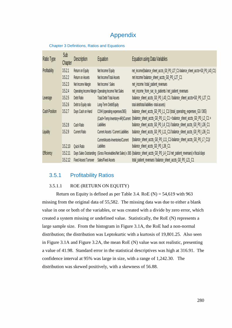
280
Appendix
Chapter 3 Definitions, Ratios and Equations
3.5.1 Profitability Ratios
3.5.1.1 ROE (RETURN ON EQUITY)
Return on Equity is defined as per Table 3.4. RoE (N) = 54,619 with 963
missing from the original data of 55,582. The missing data was due to either a blank
value in one or both of the variables, or was created with a divide by zero error, which
created a system missing or undefined value. Statistically, the RoE (N) represents a
large sample size. From the histogram in Figure 3.1A, the RoE had a non-normal
distribution; the distribution was Leptokurtic with a kurtosis of 19,801.25. Also seen
in Figure 3.1A and Figure 3.2A, the mean RoE (N) value was not realistic, presenting
a value of 41.98. Standard error in the statistical descriptives was high at 316.91. The
confidence interval at 95% was large in size, with a range of 1,242.30. The
distribution was skewed positively, with a skewness of 56.88.
Ratio Type Sub
ChapterDescription Equation Equation using Data Variables
Profitability 3.5.2.1 Return on Equity Net Income/ Equity net_income/(balance_sheet_accts_G0_P0_L27_C1-balance_sheet_accts+G0_P0_L43_C1)
3.5.2.2 Return on Assets Net Income/Total Assets net income/ balance_sheet_accts_G0_P0_L27_C1
3.5.2.3 Net Income Margin Net Income/ Sales net_income / total_patient_revenues
3.5.2.4 Operating Income Margin Operating Income/ Net Sales net_income_from_svc_to_patients / net_patient_revenues
Leverage 3.5.2.5 Debt Ratio Total Debt/ Total Assets balance_sheet_accts_G0_P0_L43_C1 / balance_sheet_accts+G0_P0_L27_C1
3.5.2.6 Debt to Equity ratio Long-Term Debt/Equity total debt/total liabilities- total assets)
Cash Position 3.5.2.7 Days Cash on Hand COH/ (operating expenses/365) balance_sheet_accts_G0_P0_L1_C1/ (total_operating_expenses_G3 / 365)
3.5.2.8 Cash Ratio
(Cash+Temp Inventory+AR)/Current
Liabilities
(balance_sheet_accts_G0_P0_L1_C1 + balance_sheet_accts_G0_P0_L2_C1 +
balance_sheet_accts_G0_P0_L4_C1) / balance_sheet_accts_G0_P0_L36_C1
Liquidity 3.5.2.9 Current Ratio Current Assets / Current Liabilities balance_sheet_accts_G0_P0_L11_C1/ balance_sheet_accts_G0_P0_L36_C1
3.5.2.10 Quick Ratio
CurrentAssets-Inventories/Current
Liabilites
(balance_sheet_accts_G0_P0_L11_C1-balance_sheet_accts_G0_P0_L7_C1)/
balance_sheet_accts_G0_P0_L36_C1
Efficiency 3.5.2.11 Days Sales Outstanding (Gross Receivables/Net Sales) x 365 (balance_sheet_accts_G0_P0_L4_C1/ net_patient_revenues) x fiscal days
3.5.2.12 Fixed Assest Turnover Sales/Fixed Assets total_patient_revenues / balance_sheet_accts_G0_P0_L21_C1
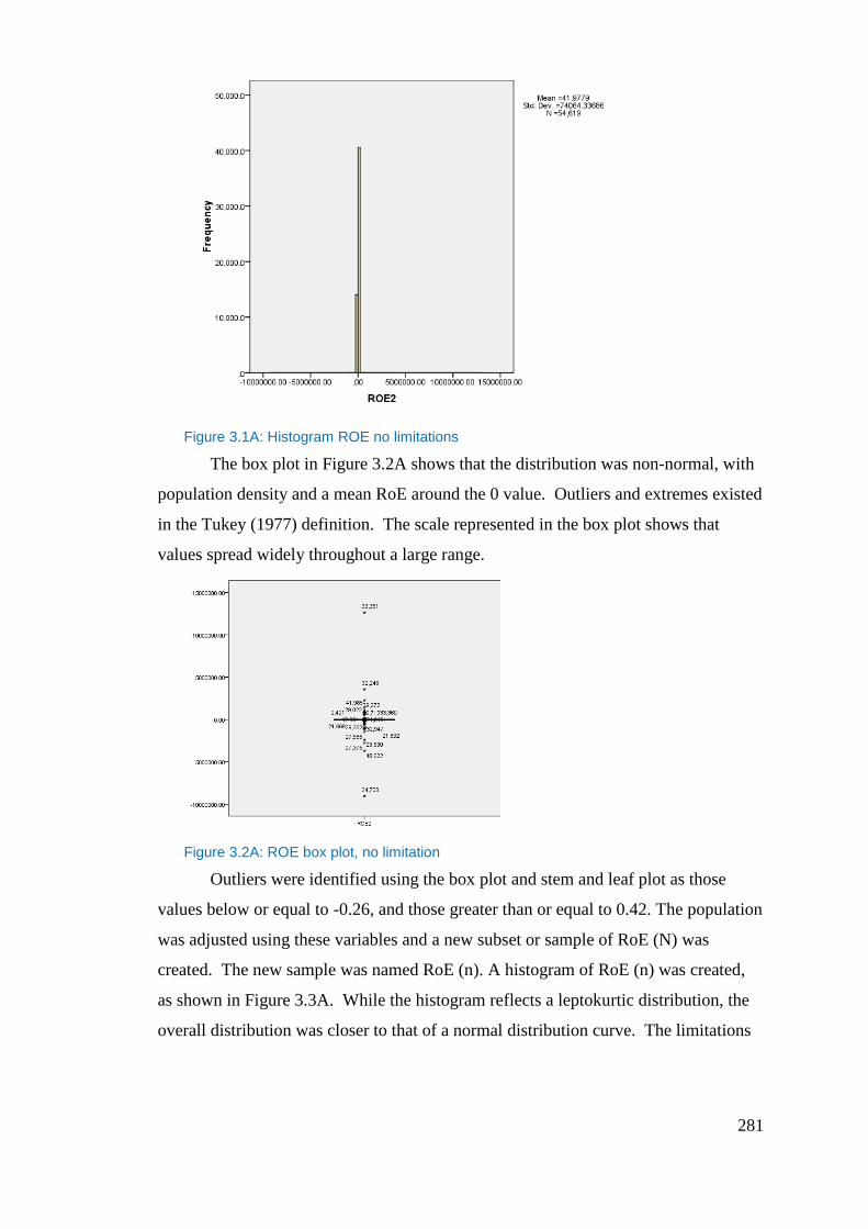
281
Figure 3.1A: Histogram ROE no limitations
The box plot in Figure 3.2A shows that the distribution was non-normal, with
population density and a mean RoE around the 0 value. Outliers and extremes existed
in the Tukey (1977) definition. The scale represented in the box plot shows that
values spread widely throughout a large range.
Figure 3.2A: ROE box plot, no limitation
Outliers were identified using the box plot and stem and leaf plot as those
values below or equal to -0.26, and those greater than or equal to 0.42. The population
was adjusted using these variables and a new subset or sample of RoE (N) was
created. The new sample was named RoE (n). A histogram of RoE (n) was created,
as shown in Figure 3.3A. While the histogram reflects a leptokurtic distribution, the
overall distribution was closer to that of a normal distribution curve. The limitations
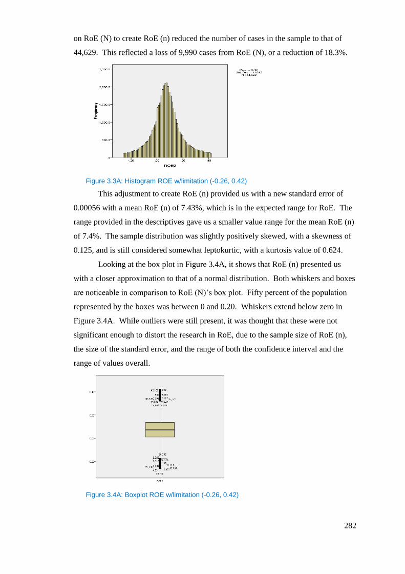
282
on RoE (N) to create RoE (n) reduced the number of cases in the sample to that of
44,629. This reflected a loss of 9,990 cases from RoE (N), or a reduction of 18.3%.
Figure 3.3A: Histogram ROE w/limitation (-0.26, 0.42)
This adjustment to create RoE (n) provided us with a new standard error of
0.00056 with a mean RoE (n) of 7.43%, which is in the expected range for RoE. The
range provided in the descriptives gave us a smaller value range for the mean RoE (n)
of 7.4%. The sample distribution was slightly positively skewed, with a skewness of
0.125, and is still considered somewhat leptokurtic, with a kurtosis value of 0.624.
Looking at the box plot in Figure 3.4A, it shows that RoE (n) presented us
with a closer approximation to that of a normal distribution. Both whiskers and boxes
are noticeable in comparison to RoE (N)’s box plot. Fifty percent of the population
represented by the boxes was between 0 and 0.20. Whiskers extend below zero in
Figure 3.4A. While outliers were still present, it was thought that these were not
significant enough to distort the research in RoE, due to the sample size of RoE (n),
the size of the standard error, and the range of both the confidence interval and the
range of values overall.
Figure 3.4A: Boxplot ROE w/limitation (-0.26, 0.42)
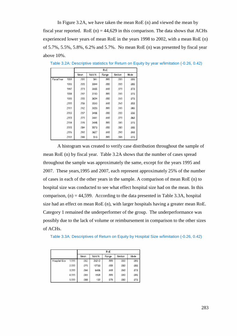
283
In Figure 3.2A, we have taken the mean RoE (n) and viewed the mean by
fiscal year reported. RoE (n) = 44,629 in this comparison. The data shows that ACHs
experienced lower years of mean RoE in the years 1998 to 2002, with a mean RoE (n)
of 5.7%, 5.5%, 5.8%, 6.2% and 5.7%. No mean RoE (n) was presented by fiscal year
above 10%.
Table 3.2A: Descriptive statistics for Return on Equity by year w/limitation (-0.26, 0.42)
A histogram was created to verify case distribution throughout the sample of
mean RoE (n) by fiscal year. Table 3.2A shows that the number of cases spread
throughout the sample was approximately the same, except for the years 1995 and
2007. These years,1995 and 2007, each represent approximately 25% of the number
of cases in each of the other years in the sample. A comparison of mean RoE (n) to
hospital size was conducted to see what effect hospital size had on the mean. In this
comparison, (n) = 44,599. According to the data presented in Table 3.3A, hospital
size had an effect on mean RoE (n), with larger hospitals having a greater mean RoE.
Category 1 remained the underperformer of the group. The underperformance was
possibly due to the lack of volume or reimbursement in comparison to the other sizes
of ACHs.
Table 3.3A: Descriptives of Return on Equity by Hospital Size w/limitation (-0.26, 0.42)
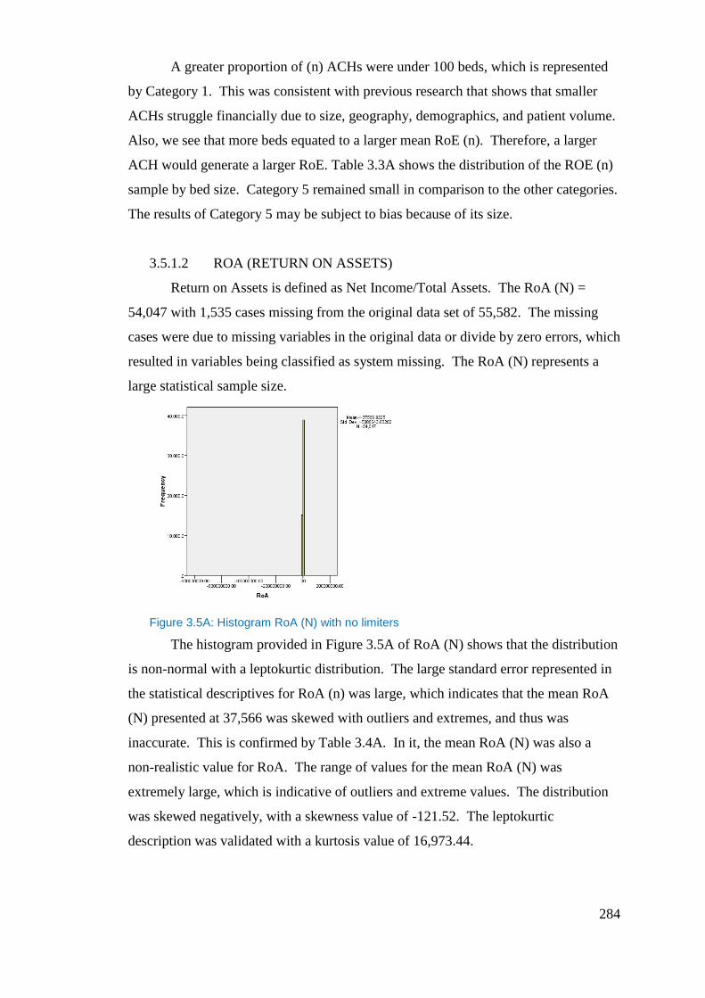
284
A greater proportion of (n) ACHs were under 100 beds, which is represented
by Category 1. This was consistent with previous research that shows that smaller
ACHs struggle financially due to size, geography, demographics, and patient volume.
Also, we see that more beds equated to a larger mean RoE (n). Therefore, a larger
ACH would generate a larger RoE. Table 3.3A shows the distribution of the ROE (n)
sample by bed size. Category 5 remained small in comparison to the other categories.
The results of Category 5 may be subject to bias because of its size.
3.5.1.2 ROA (RETURN ON ASSETS)
Return on Assets is defined as Net Income/Total Assets. The RoA (N) =
54,047 with 1,535 cases missing from the original data set of 55,582. The missing
cases were due to missing variables in the original data or divide by zero errors, which
resulted in variables being classified as system missing. The RoA (N) represents a
large statistical sample size.
Figure 3.5A: Histogram RoA (N) with no limiters
The histogram provided in Figure 3.5A of RoA (N) shows that the distribution
is non-normal with a leptokurtic distribution. The large standard error represented in
the statistical descriptives for RoA (n) was large, which indicates that the mean RoA
(N) presented at 37,566 was skewed with outliers and extremes, and thus was
inaccurate. This is confirmed by Table 3.4A. In it, the mean RoA (N) was also a
non-realistic value for RoA. The range of values for the mean RoA (N) was
extremely large, which is indicative of outliers and extreme values. The distribution
was skewed negatively, with a skewness value of -121.52. The leptokurtic
description was validated with a kurtosis value of 16,973.44.
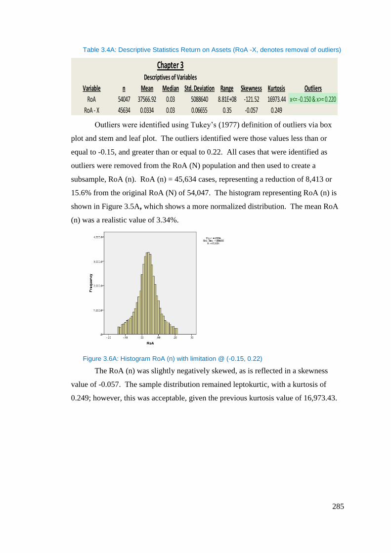
285
Table 3.4A: Descriptive Statistics Return on Assets (RoA -X, denotes removal of outliers)
Outliers were identified using Tukey’s (1977) definition of outliers via box
plot and stem and leaf plot. The outliers identified were those values less than or
equal to -0.15, and greater than or equal to 0.22. All cases that were identified as
outliers were removed from the RoA (N) population and then used to create a
subsample, RoA (n). RoA (n) = 45,634 cases, representing a reduction of 8,413 or
15.6% from the original RoA (N) of 54,047. The histogram representing RoA (n) is
shown in Figure 3.5A, which shows a more normalized distribution. The mean RoA
(n) was a realistic value of 3.34%.
Figure 3.6A: Histogram RoA (n) with limitation @ (-0.15, 0.22)
The RoA (n) was slightly negatively skewed, as is reflected in a skewness
value of -0.057. The sample distribution remained leptokurtic, with a kurtosis of
0.249; however, this was acceptable, given the previous kurtosis value of 16,973.43.
Chapter 3Descriptives of Variables
Variable n Mean Median Std. Deviation Range Skewness Kurtosis Outliers
RoA 54047 37566.92 0.03 5088640 8.81E+08 -121.52 16973.44 x<= -0.150 & x>= 0.220
RoA - X 45634 0.0334 0.03 0.06655 0.35 -0.057 0.249
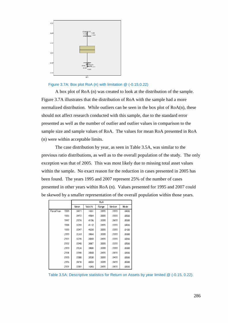
286
Figure 3.7A: Box plot RoA (n) with limitation @ (-0.15,0.22)
A box plot of RoA (n) was created to look at the distribution of the sample.
Figure 3.7A illustrates that the distribution of RoA with the sample had a more
normalized distribution. While outliers can be seen in the box plot of RoA(n), these
should not affect research conducted with this sample, due to the standard error
presented as well as the number of outlier and outlier values in comparison to the
sample size and sample values of RoA. The values for mean RoA presented in RoA
(n) were within acceptable limits.
The case distribution by year, as seen in Table 3.5A, was similar to the
previous ratio distributions, as well as to the overall population of the study. The only
exception was that of 2005. This was most likely due to missing total asset values
within the sample. No exact reason for the reduction in cases presented in 2005 has
been found. The years 1995 and 2007 represent 25% of the number of cases
presented in other years within RoA (n). Values presented for 1995 and 2007 could
be skewed by a smaller representation of the overall population within those years.
Table 3.5A: Descriptive statistics for Return on Assets by year limited @ (-0.15, 0.22).
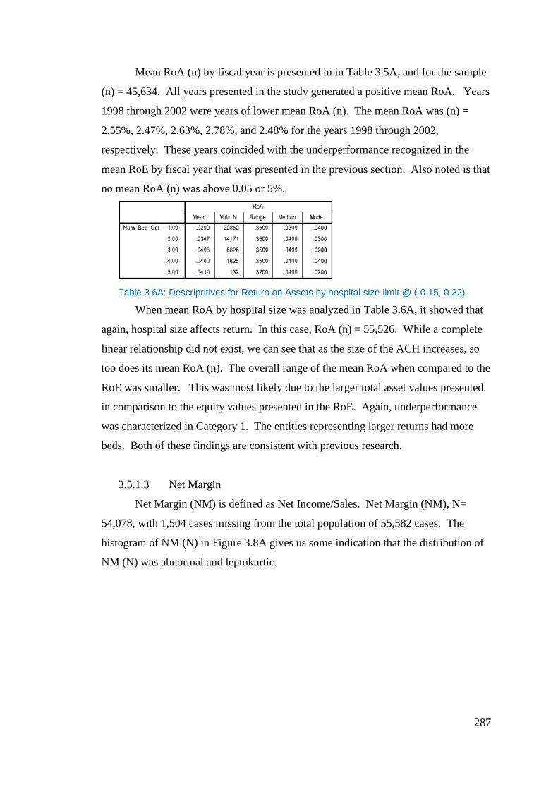
287
Mean RoA (n) by fiscal year is presented in in Table 3.5A, and for the sample
(n) = 45,634. All years presented in the study generated a positive mean RoA. Years
1998 through 2002 were years of lower mean RoA (n). The mean RoA was (n) =
2.55%, 2.47%, 2.63%, 2.78%, and 2.48% for the years 1998 through 2002,
respectively. These years coincided with the underperformance recognized in the
mean RoE by fiscal year that was presented in the previous section. Also noted is that
no mean RoA (n) was above 0.05 or 5%.
Table 3.6A: Descripritives for Return on Assets by hospital size limit @ (-0.15, 0.22).
When mean RoA by hospital size was analyzed in Table 3.6A, it showed that
again, hospital size affects return. In this case, RoA (n) = 55,526. While a complete
linear relationship did not exist, we can see that as the size of the ACH increases, so
too does its mean RoA (n). The overall range of the mean RoA when compared to the
RoE was smaller. This was most likely due to the larger total asset values presented
in comparison to the equity values presented in the RoE. Again, underperformance
was characterized in Category 1. The entities representing larger returns had more
beds. Both of these findings are consistent with previous research.
3.5.1.3 Net Margin
Net Margin (NM) is defined as Net Income/Sales. Net Margin (NM), N=
54,078, with 1,504 cases missing from the total population of 55,582 cases. The
histogram of NM (N) in Figure 3.8A gives us some indication that the distribution of
NM (N) was abnormal and leptokurtic.
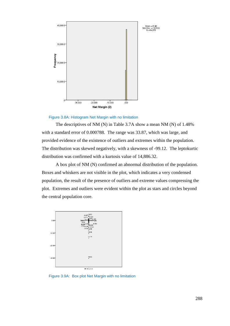
288
Figure 3.8A: Histogram Net Margin with no limitation
The descriptives of NM (N) in Table 3.7A show a mean NM (N) of 1.48%
with a standard error of 0.000788. The range was 33.87, which was large, and
provided evidence of the existence of outliers and extremes within the population.
The distribution was skewed negatively, with a skewness of -99.12. The leptokurtic
distribution was confirmed with a kurtosis value of 14,886.32.
A box plot of NM (N) confirmed an abnormal distribution of the population.
Boxes and whiskers are not visible in the plot, which indicates a very condensed
population, the result of the presence of outliers and extreme values compressing the
plot. Extremes and outliers were evident within the plot as stars and circles beyond
the central population core.
Figure 3.9A: Box plot Net Margin with no limitation
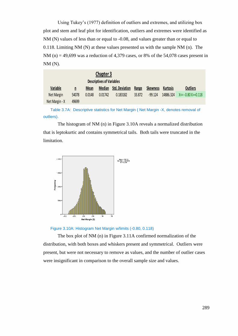
289
Using Tukey’s (1977) definition of outliers and extremes, and utilizing box
plot and stem and leaf plot for identification, outliers and extremes were identified as
NM (N) values of less than or equal to -0.08, and values greater than or equal to
0.118. Limiting NM (N) at these values presented us with the sample NM (n). The
NM (n) = 49,699 was a reduction of 4,379 cases, or 8% of the 54,078 cases present in
NM (N).
Table 3.7A: Descriptive statistics for Net Margin ( Net Margin -X, denotes removal of
outliers).
The histogram of NM (n) in Figure 3.10A reveals a normalized distribution
that is leptokurtic and contains symmetrical tails. Both tails were truncated in the
limitation.
Figure 3.10A: Histogram Net Margin w/limits (-0.80, 0.118)
The box plot of NM (n) in Figure 3.11A confirmed normalization of the
distribution, with both boxes and whiskers present and symmetrical. Outliers were
present, but were not necessary to remove as values, and the number of outlier cases
were insignificant in comparison to the overall sample size and values.
Chapter 3Descriptives of Variables
Variable n Mean Median Std. Deviation Range Skewness Kurtosis Outliers
Net Margin 54078 0.0148 0.01742 0.183182 33.872 -99.124 14886.324 X<= -0.80 X>=0.118
Net Margin - X 49699
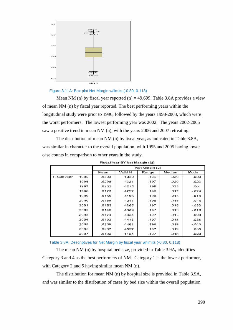
290
Figure 3.11A: Box plot Net Margin w/limits (-0.80, 0.118)
Mean NM (n) by fiscal year reported (n) = 49,699. Table 3.8A provides a view
of mean NM (n) by fiscal year reported. The best performing years within the
longitudinal study were prior to 1996, followed by the years 1998-2003, which were
the worst performers. The lowest performing year was 2002. The years 2002-2005
saw a positive trend in mean NM (n), with the years 2006 and 2007 retreating.
The distribution of mean NM (n) by fiscal year, as indicated in Table 3.8A,
was similar in character to the overall population, with 1995 and 2005 having lower
case counts in comparison to other years in the study.
Table 3.8A: Descriptives for Net Margin by fiscal year w/limits (-0.80, 0.118)
The mean NM (n) by hospital bed size, provided in Table 3.9A, identifies
Category 3 and 4 as the best performers of NM. Category 1 is the lowest performer,
with Category 2 and 5 having similar mean NM (n).
The distribution for mean NM (n) by hospital size is provided in Table 3.9A,
and was similar to the distribution of cases by bed size within the overall population
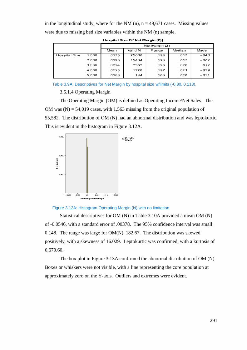
291
in the longitudinal study, where for the NM (n), n = 49,671 cases. Missing values
were due to missing bed size variables within the NM (n) sample.
Table 3.9A: Descriptives for Net Margin by hospital size w/limits (-0.80, 0.118).
3.5.1.4 Operating Margin
The Operating Margin (OM) is defined as Operating Income/Net Sales. The
OM was (N) = 54,019 cases, with 1,563 missing from the original population of
55,582. The distribution of OM (N) had an abnormal distribution and was leptokurtic.
This is evident in the histogram in Figure 3.12A.
Figure 3.12A: Histogram Operating Margin (N) with no limitation
Statistical descriptives for OM (N) in Table 3.10A provided a mean OM (N)
of -0.0546, with a standard error of .00378. The 95% confidence interval was small:
0.148. The range was large for OM(N), 182.67. The distribution was skewed
positively, with a skewness of 16.029. Leptokurtic was confirmed, with a kurtosis of
6,679.60.
The box plot in Figure 3.13A confirmed the abnormal distribution of OM (N).
Boxes or whiskers were not visible, with a line representing the core population at
approximately zero on the Y-axis. Outliers and extremes were evident.
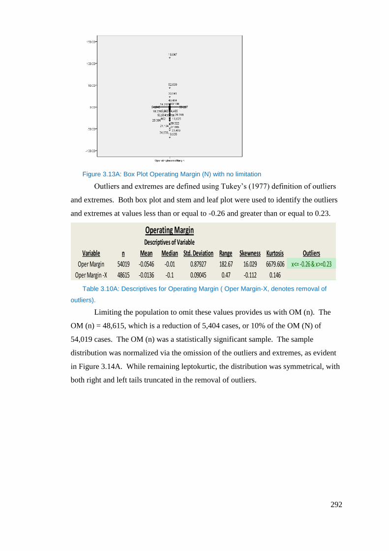
292
Figure 3.13A: Box Plot Operating Margin (N) with no limitation
Outliers and extremes are defined using Tukey’s (1977) definition of outliers
and extremes. Both box plot and stem and leaf plot were used to identify the outliers
and extremes at values less than or equal to -0.26 and greater than or equal to 0.23.
Table 3.10A: Descriptives for Operating Margin ( Oper Margin-X, denotes removal of
outliers).
Limiting the population to omit these values provides us with OM (n). The
OM (n) = 48,615, which is a reduction of 5,404 cases, or 10% of the OM (N) of
54,019 cases. The OM (n) was a statistically significant sample. The sample
distribution was normalized via the omission of the outliers and extremes, as evident
in Figure 3.14A. While remaining leptokurtic, the distribution was symmetrical, with
both right and left tails truncated in the removal of outliers.
Operating MarginDescriptives of Variable
Variable n Mean Median Std. Deviation Range Skewness Kurtosis Outliers
Oper Margin 54019 -0.0546 -0.01 0.87927 182.67 16.029 6679.606 x<= -0.26 & x>=0.23
Oper Margin -X 48615 -0.0136 -0.1 0.09045 0.47 -0.112 0.146
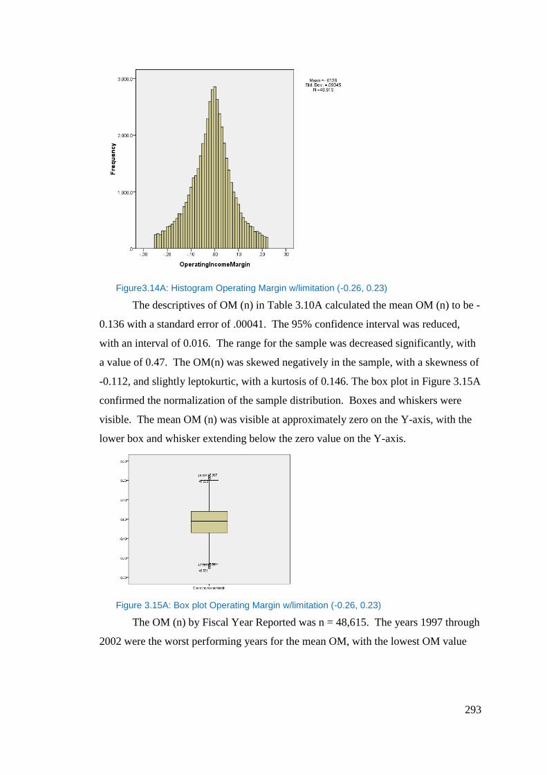
293
Figure3.14A: Histogram Operating Margin w/limitation (-0.26, 0.23)
The descriptives of OM (n) in Table 3.10A calculated the mean OM (n) to be -
0.136 with a standard error of .00041. The 95% confidence interval was reduced,
with an interval of 0.016. The range for the sample was decreased significantly, with
a value of 0.47. The OM(n) was skewed negatively in the sample, with a skewness of
-0.112, and slightly leptokurtic, with a kurtosis of 0.146. The box plot in Figure 3.15A
confirmed the normalization of the sample distribution. Boxes and whiskers were
visible. The mean OM (n) was visible at approximately zero on the Y-axis, with the
lower box and whisker extending below the zero value on the Y-axis.
Figure 3.15A: Box plot Operating Margin w/limitation (-0.26, 0.23)
The OM (n) by Fiscal Year Reported was n = 48,615. The years 1997 through
2002 were the worst performing years for the mean OM, with the lowest OM value
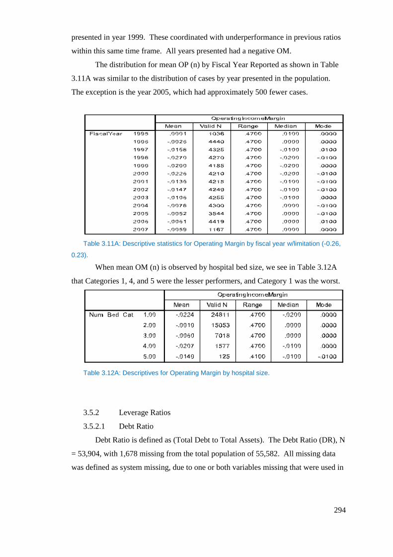
294
presented in year 1999. These coordinated with underperformance in previous ratios
within this same time frame. All years presented had a negative OM.
The distribution for mean OP (n) by Fiscal Year Reported as shown in Table
3.11A was similar to the distribution of cases by year presented in the population.
The exception is the year 2005, which had approximately 500 fewer cases.
Table 3.11A: Descriptive statistics for Operating Margin by fiscal year w/limitation (-0.26,
0.23).
When mean OM (n) is observed by hospital bed size, we see in Table 3.12A
that Categories 1, 4, and 5 were the lesser performers, and Category 1 was the worst.
Table 3.12A: Descriptives for Operating Margin by hospital size.
3.5.2 Leverage Ratios
3.5.2.1 Debt Ratio
Debt Ratio is defined as (Total Debt to Total Assets). The Debt Ratio (DR), N
= 53,904, with 1,678 missing from the total population of 55,582. All missing data
was defined as system missing, due to one or both variables missing that were used in
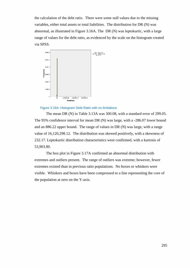
295
the calculation of the debt ratio. There were some null values due to the missing
variables, either total assets or total liabilities. The distribution for DR (N) was
abnormal, as illustrated in Figure 3.16A. The DR (N) was leptokurtic, with a large
range of values for the debt ratio, as evidenced by the scale on the histogram created
via SPSS.
Figure 3.16A: Histogram Debt Ratio with no limitations
The mean DR (N) in Table 3.13A was 300.08, with a standard error of 299.05.
The 95% confidence interval for mean DR (N) was large, with a -286.07 lower bound
and an 886.22 upper bound. The range of values in DR (N) was large, with a range
value of 16,120,298.12. The distribution was skewed positively, with a skewness of
232.17. Leptokurtic distribution characteristics were confirmed, with a kurtosis of
53,903.80.
The box plot in Figure 3.17A confirmed an abnormal distribution with
extremes and outliers present. The range of outliers was extreme; however, fewer
extremes existed than in previous ratio populations. No boxes or whiskers were
visible. Whiskers and boxes have been compressed to a line representing the core of
the population at zero on the Y-axis.
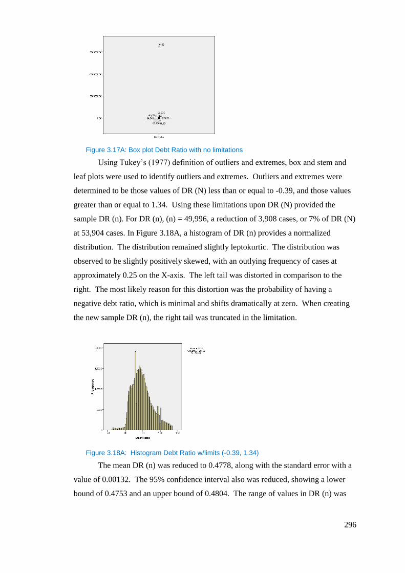
296
Figure 3.17A: Box plot Debt Ratio with no limitations
Using Tukey’s (1977) definition of outliers and extremes, box and stem and
leaf plots were used to identify outliers and extremes. Outliers and extremes were
determined to be those values of DR (N) less than or equal to -0.39, and those values
greater than or equal to 1.34. Using these limitations upon DR (N) provided the
sample DR (n). For DR (n), (n) = 49,996, a reduction of 3,908 cases, or 7% of DR (N)
at 53,904 cases. In Figure 3.18A, a histogram of DR (n) provides a normalized
distribution. The distribution remained slightly leptokurtic. The distribution was
observed to be slightly positively skewed, with an outlying frequency of cases at
approximately 0.25 on the X-axis. The left tail was distorted in comparison to the
right. The most likely reason for this distortion was the probability of having a
negative debt ratio, which is minimal and shifts dramatically at zero. When creating
the new sample DR (n), the right tail was truncated in the limitation.
Figure 3.18A: Histogram Debt Ratio w/limits (-0.39, 1.34)
The mean DR (n) was reduced to 0.4778, along with the standard error with a
value of 0.00132. The 95% confidence interval also was reduced, showing a lower
bound of 0.4753 and an upper bound of 0.4804. The range of values in DR (n) was

297
decreased to 1.71. The distribution remains positively skewed, and was confirmed
with a skewness of 0.5. A reduction in the leptokurtic characteristic was confirmed,
with a kurtosis of .084, in comparison to the previous kurtosis value presented in DR
(N) of 53,908.80.
Table 3.13A: Descriptive statistics for Debt Ratio (Debt Ratio-X, denotes removal of
outliers).
The box plot in Figure 3.19A of DR (n) confirmed normalization of the
distribution of the sample. Boxes and whiskers were visible in comparison to the box
plot presented of DR (N). Outliers were present beyond the upper and lower
whiskers. The outliers in this sample should not affect the calculation of mean DR (n).
Figure 3.19A: Box plot Debt Ratio w/limits (-0.39, 1.34)
The mean DR (n) by Fiscal Year Reported in Table 3.14A gave evidence of an
increasing mean DR (n) from the years 1995-2002, with a reduction from that time
until 2007. No mean DR(n) for any Fiscal Year was less than 0.45, with the greatest
value presented in 2007, with a Debt Ratio of approximately 0.5. The years 1995
through 2002 matched previous time frames for poorer values of financial ratios.
DR (n) by Fiscal Year Reported, n = 49,996, is presented in Table 3.14A,
below. The distribution matches all years in frequency of cases except for 2005,
Debt RatioDescriptives of Variable
Variable n Mean Median Std. Deviation Range Skewness Kurtosis Outliers
Debt Ratio 53904 300.075 0.45 69431.498 16120298 232.172 53903.798 X<=-0.39& X>=1.34
Debt Ratio - X 49996 0.4778 0.44 0.29558 1.71 0.5 0.084
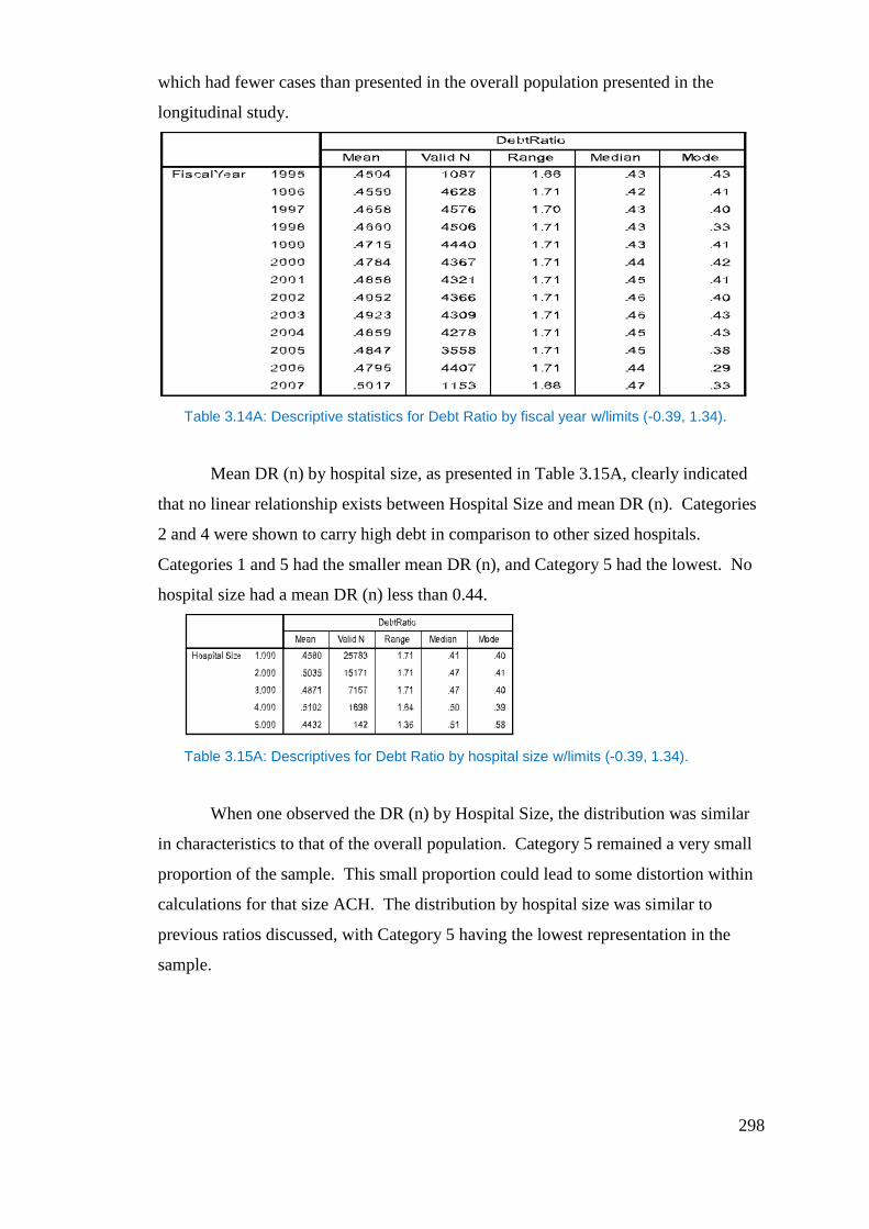
298
which had fewer cases than presented in the overall population presented in the
longitudinal study.
Table 3.14A: Descriptive statistics for Debt Ratio by fiscal year w/limits (-0.39, 1.34).
Mean DR (n) by hospital size, as presented in Table 3.15A, clearly indicated
that no linear relationship exists between Hospital Size and mean DR (n). Categories
2 and 4 were shown to carry high debt in comparison to other sized hospitals.
Categories 1 and 5 had the smaller mean DR (n), and Category 5 had the lowest. No
hospital size had a mean DR (n) less than 0.44.
Table 3.15A: Descriptives for Debt Ratio by hospital size w/limits (-0.39, 1.34).
When one observed the DR (n) by Hospital Size, the distribution was similar
in characteristics to that of the overall population. Category 5 remained a very small
proportion of the sample. This small proportion could lead to some distortion within
calculations for that size ACH. The distribution by hospital size was similar to
previous ratios discussed, with Category 5 having the lowest representation in the
sample.
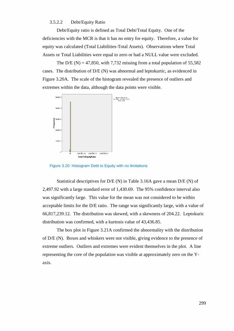
299
3.5.2.2 Debt/Equity Ratio
Debt/Equity ratio is defined as Total Debt/Total Equity. One of the
deficiencies with the MCR is that it has no entry for equity. Therefore, a value for
equity was calculated (Total Liabilities-Total Assets). Observations where Total
Assets or Total Liabilities were equal to zero or had a NULL value were excluded.
The D/E (N) = 47,850, with 7,732 missing from a total population of 55,582
cases. The distribution of D/E (N) was abnormal and leptokurtic, as evidenced in
Figure 3.20A. The scale of the histogram revealed the presence of outliers and
extremes within the data, although the data points were visible.
Figure 3.20: Histogram Debt to Equity with no limitations
Statistical descriptives for D/E (N) in Table 3.16A gave a mean D/E (N) of
2,497.92 with a large standard error of 1,430.69. The 95% confidence interval also
was significantly large. This value for the mean was not considered to be within
acceptable limits for the D/E ratio. The range was significantly large, with a value of
66,817,239.12. The distribution was skewed, with a skewness of 204.22. Leptokuric
distribution was confirmed, with a kurtosis value of 43,436.85.
The box plot in Figure 3.21A confirmed the abnormality with the distribution
of D/E (N). Boxes and whiskers were not visible, giving evidence to the presence of
extreme outliers. Outliers and extremes were evident themselves in the plot. A line
representing the core of the population was visible at approximately zero on the Y-
axis.
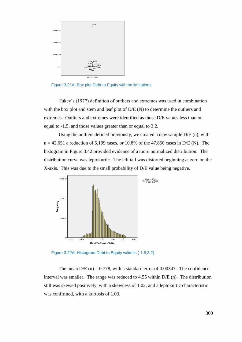
300
Figure 3.21A: Box plot Debt to Equity with no limitations
Tukey’s (1977) definition of outliers and extremes was used in combination
with the box plot and stem and leaf plot of D/E (N) to determine the outliers and
extremes. Outliers and extremes were identified as those D/E values less than or
equal to -1.5, and those values greater than or equal to 3.2.
Using the outliers defined previously, we created a new sample D/E (n), with
n = 42,651 a reduction of 5,199 cases, or 10.8% of the 47,850 cases in D/E (N). The
histogram in Figure 3.42 provided evidence of a more normalized distribution. The
distribution curve was leptokurtic. The left tail was distorted beginning at zero on the
X-axis. This was due to the small probability of D/E value being negative.
Figure 3.22A: Histogram Debt to Equity w/limits (-1.5,3.2)
The mean D/E (n) = 0.778, with a standard error of 0.00347. The confidence
interval was smaller. The range was reduced to 4.55 within D/E (n). The distribution
still was skewed positively, with a skewness of 1.02, and a leptokurtic characteristic
was confirmed, with a kurtosis of 1.03.
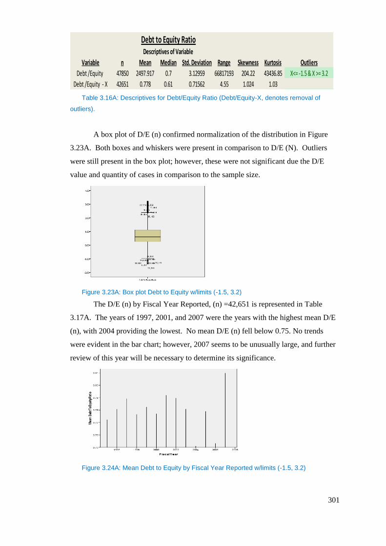
301
Table 3.16A: Descriptives for Debt/Equity Ratio (Debt/Equity-X, denotes removal of
outliers).
A box plot of D/E (n) confirmed normalization of the distribution in Figure
3.23A. Both boxes and whiskers were present in comparison to D/E (N). Outliers
were still present in the box plot; however, these were not significant due the D/E
value and quantity of cases in comparison to the sample size.
Figure 3.23A: Box plot Debt to Equity w/limits (-1.5, 3.2)
The D/E (n) by Fiscal Year Reported, (n) =42,651 is represented in Table
3.17A. The years of 1997, 2001, and 2007 were the years with the highest mean D/E
(n), with 2004 providing the lowest. No mean D/E (n) fell below 0.75. No trends
were evident in the bar chart; however, 2007 seems to be unusually large, and further
review of this year will be necessary to determine its significance.
Figure 3.24A: Mean Debt to Equity by Fiscal Year Reported w/limits (-1.5, 3.2)
Debt to Equity RatioDescriptives of Variable
Variable n Mean Median Std. Deviation Range Skewness Kurtosis Outliers
Debt /Equity 47850 2497.917 0.7 3.12959 66817193 204.22 43436.85 X<= -1.5 & X >= 3.2
Debt /Equity - X 42651 0.778 0.61 0.71562 4.55 1.024 1.03
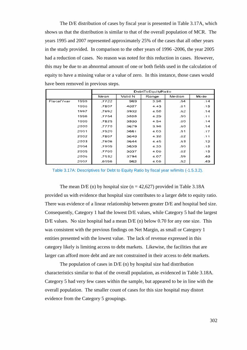
302
The D/E distribution of cases by fiscal year is presented in Table 3.17A, which
shows us that the distribution is similar to that of the overall population of MCR. The
years 1995 and 2007 represented approximately 25% of the cases that all other years
in the study provided. In comparison to the other years of 1996 -2006, the year 2005
had a reduction of cases. No reason was noted for this reduction in cases. However,
this may be due to an abnormal amount of one or both fields used in the calculation of
equity to have a missing value or a value of zero. In this instance, those cases would
have been removed in previous steps.
Table 3.17A: Descriptives for Debt to Equity Ratio by fiscal year w/limits (-1.5.3.2).
The mean D/E (n) by hospital size (n = 42,627) provided in Table 3.18A
provided us with evidence that hospital size contributes to a larger debt to equity ratio.
There was evidence of a linear relationship between greater D/E and hospital bed size.
Consequently, Category 1 had the lowest D/E values, while Category 5 had the largest
D/E values. No size hospital had a mean D/E (n) below 0.70 for any one size. This
was consistent with the previous findings on Net Margin, as small or Category 1
entities presented with the lowest value. The lack of revenue expressed in this
category likely is limiting access to debt markets. Likewise, the facilities that are
larger can afford more debt and are not constrained in their access to debt markets.
The population of cases in D/E (n) by hospital size had distribution
characteristics similar to that of the overall population, as evidenced in Table 3.18A.
Category 5 had very few cases within the sample, but appeared to be in line with the
overall population. The smaller count of cases for this size hospital may distort
evidence from the Category 5 groupings.
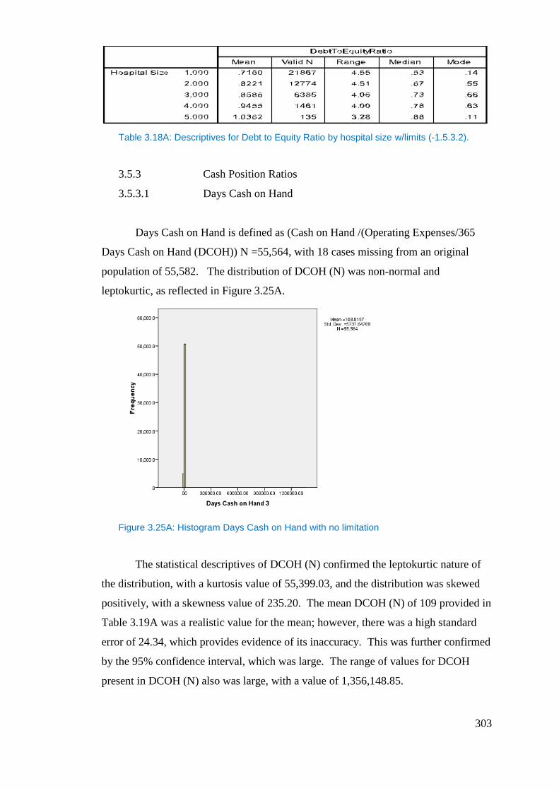
303
Table 3.18A: Descriptives for Debt to Equity Ratio by hospital size w/limits (-1.5.3.2).
3.5.3 Cash Position Ratios
3.5.3.1 Days Cash on Hand
Days Cash on Hand is defined as (Cash on Hand /(Operating Expenses/365
Days Cash on Hand (DCOH)) N =55,564, with 18 cases missing from an original
population of 55,582. The distribution of DCOH (N) was non-normal and
leptokurtic, as reflected in Figure 3.25A.
Figure 3.25A: Histogram Days Cash on Hand with no limitation
The statistical descriptives of DCOH (N) confirmed the leptokurtic nature of
the distribution, with a kurtosis value of 55,399.03, and the distribution was skewed
positively, with a skewness value of 235.20. The mean DCOH (N) of 109 provided in
Table 3.19A was a realistic value for the mean; however, there was a high standard
error of 24.34, which provides evidence of its inaccuracy. This was further confirmed
by the 95% confidence interval, which was large. The range of values for DCOH
present in DCOH (N) also was large, with a value of 1,356,148.85.
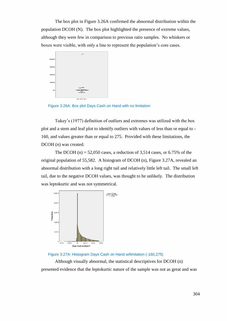
304
The box plot in Figure 3.26A confirmed the abnormal distribution within the
population DCOH (N). The box plot highlighted the presence of extreme values,
although they were few in comparison to previous ratio samples. No whiskers or
boxes were visible, with only a line to represent the population’s core cases.
Figure 3.26A: Box plot Days Cash on Hand with no limitation
Tukey’s (1977) definition of outliers and extremes was utilized with the box
plot and a stem and leaf plot to identify outliers with values of less than or equal to -
160, and values greater than or equal to 275. Provided with these limitations, the
DCOH (n) was created.
The DCOH (n) = 52,050 cases, a reduction of 3,514 cases, or 6.75% of the
original population of 55,582. A histogram of DCOH (n), Figure 3.27A, revealed an
abnormal distribution with a long right tail and relatively little left tail. The small left
tail, due to the negative DCOH values, was thought to be unlikely. The distribution
was leptokurtic and was not symmetrical.
Figure 3.27A: Histogram Days Cash on Hand w/limitation (-160,275)
Although visually abnormal, the statistical descriptives for DCOH (n)
presented evidence that the leptokurtic nature of the sample was not as great and was
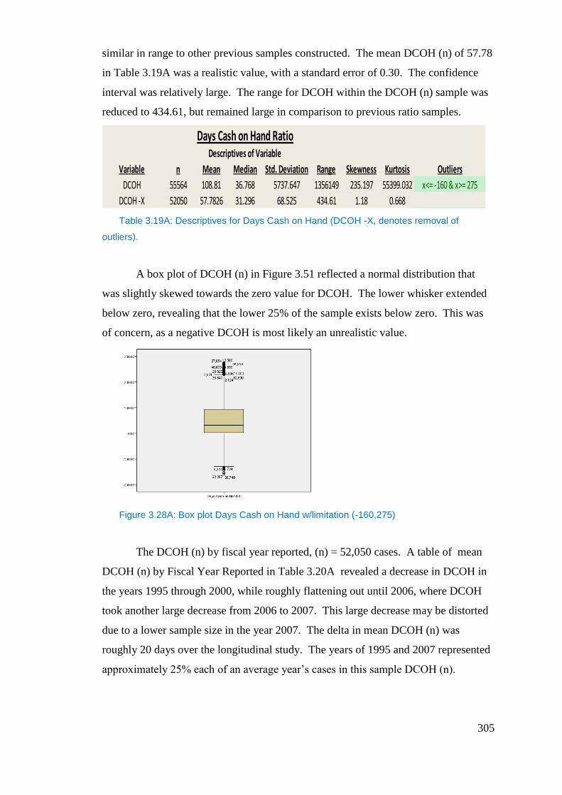
305
similar in range to other previous samples constructed. The mean DCOH (n) of 57.78
in Table 3.19A was a realistic value, with a standard error of 0.30. The confidence
interval was relatively large. The range for DCOH within the DCOH (n) sample was
reduced to 434.61, but remained large in comparison to previous ratio samples.
Table 3.19A: Descriptives for Days Cash on Hand (DCOH -X, denotes removal of
outliers).
A box plot of DCOH (n) in Figure 3.51 reflected a normal distribution that
was slightly skewed towards the zero value for DCOH. The lower whisker extended
below zero, revealing that the lower 25% of the sample exists below zero. This was
of concern, as a negative DCOH is most likely an unrealistic value.
Figure 3.28A: Box plot Days Cash on Hand w/limitation (-160,275)
The DCOH (n) by fiscal year reported, (n) = 52,050 cases. A table of mean
DCOH (n) by Fiscal Year Reported in Table 3.20A revealed a decrease in DCOH in
the years 1995 through 2000, while roughly flattening out until 2006, where DCOH
took another large decrease from 2006 to 2007. This large decrease may be distorted
due to a lower sample size in the year 2007. The delta in mean DCOH (n) was
roughly 20 days over the longitudinal study. The years of 1995 and 2007 represented
approximately 25% each of an average year’s cases in this sample DCOH (n).
Days Cash on Hand RatioDescriptives of Variable
Variable n Mean Median Std. Deviation Range Skewness Kurtosis Outliers
DCOH 55564 108.81 36.768 5737.647 1356149 235.197 55399.032 x<= -160 & x>= 275
DCOH -X 52050 57.7826 31.296 68.525 434.61 1.18 0.668
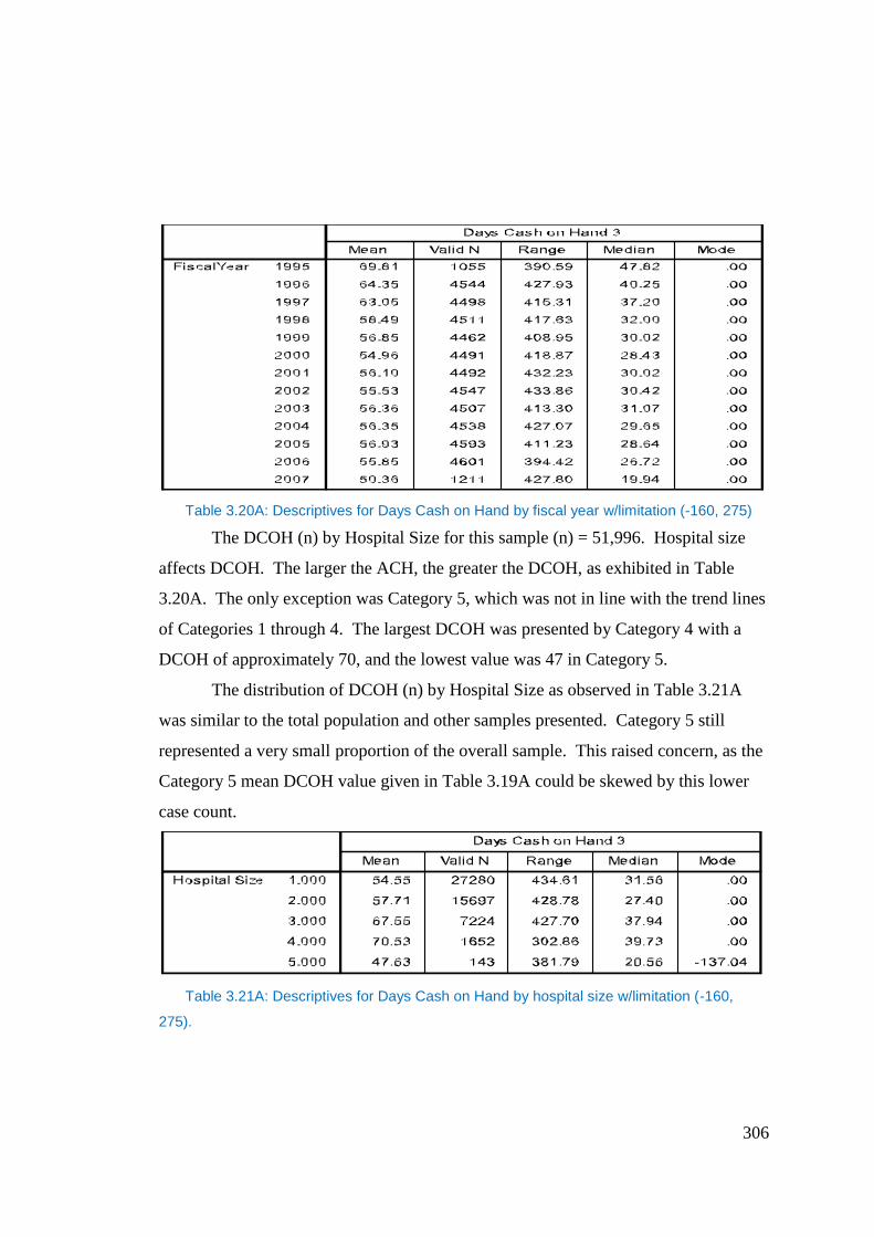
306
Table 3.20A: Descriptives for Days Cash on Hand by fiscal year w/limitation (-160, 275)
The DCOH (n) by Hospital Size for this sample (n) = 51,996. Hospital size
affects DCOH. The larger the ACH, the greater the DCOH, as exhibited in Table
3.20A. The only exception was Category 5, which was not in line with the trend lines
of Categories 1 through 4. The largest DCOH was presented by Category 4 with a
DCOH of approximately 70, and the lowest value was 47 in Category 5.
The distribution of DCOH (n) by Hospital Size as observed in Table 3.21A
was similar to the total population and other samples presented. Category 5 still
represented a very small proportion of the overall sample. This raised concern, as the
Category 5 mean DCOH value given in Table 3.19A could be skewed by this lower
case count.
Table 3.21A: Descriptives for Days Cash on Hand by hospital size w/limitation (-160,
275).
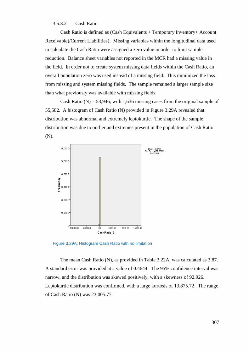
307
3.5.3.2 Cash Ratio
Cash Ratio is defined as (Cash Equivalents + Temporary Inventory+ Account
Receivable)/Current Liabilities). Missing variables within the longitudinal data used
to calculate the Cash Ratio were assigned a zero value in order to limit sample
reduction. Balance sheet variables not reported in the MCR had a missing value in
the field. In order not to create system missing data fields within the Cash Ratio, an
overall population zero was used instead of a missing field. This minimized the loss
from missing and system missing fields. The sample remained a larger sample size
than what previously was available with missing fields.
Cash Ratio (N) = 53,946, with 1,636 missing cases from the original sample of
55,582. A histogram of Cash Ratio (N) provided in Figure 3.29A revealed that
distribution was abnormal and extremely leptokurtic. The shape of the sample
distribution was due to outlier and extremes present in the population of Cash Ratio
(N).
Figure 3.29A: Histogram Cash Ratio with no limitation
The mean Cash Ratio (N), as provided in Table 3.22A, was calculated as 3.87.
A standard error was provided at a value of 0.4644. The 95% confidence interval was
narrow, and the distribution was skewed positively, with a skewness of 92.926.
Leptokurtic distribution was confirmed, with a large kurtosis of 13,875.72. The range
of Cash Ratio (N) was 23,005.77.
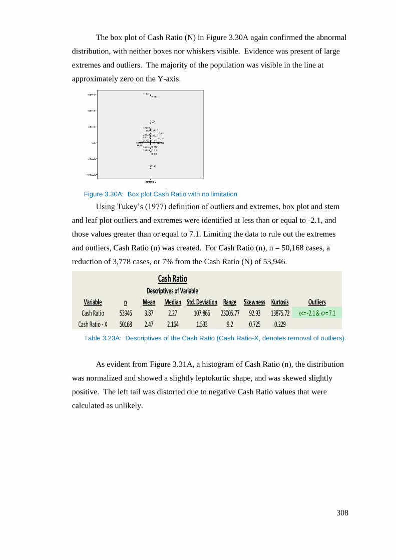
308
The box plot of Cash Ratio (N) in Figure 3.30A again confirmed the abnormal
distribution, with neither boxes nor whiskers visible. Evidence was present of large
extremes and outliers. The majority of the population was visible in the line at
approximately zero on the Y-axis.
Figure 3.30A: Box plot Cash Ratio with no limitation
Using Tukey’s (1977) definition of outliers and extremes, box plot and stem
and leaf plot outliers and extremes were identified at less than or equal to -2.1, and
those values greater than or equal to 7.1. Limiting the data to rule out the extremes
and outliers, Cash Ratio (n) was created. For Cash Ratio (n), n = 50,168 cases, a
reduction of 3,778 cases, or 7% from the Cash Ratio (N) of 53,946.
Table 3.23A: Descriptives of the Cash Ratio (Cash Ratio-X, denotes removal of outliers).
As evident from Figure 3.31A, a histogram of Cash Ratio (n), the distribution
was normalized and showed a slightly leptokurtic shape, and was skewed slightly
positive. The left tail was distorted due to negative Cash Ratio values that were
calculated as unlikely.
Cash RatioDescriptives of Variable
Variable n Mean Median Std. Deviation Range Skewness Kurtosis Outliers
Cash Ratio 53946 3.87 2.27 107.866 23005.77 92.93 13875.72 x<= -2.1 & x>= 7.1
Cash Ratio - X 50168 2.47 2.164 1.533 9.2 0.725 0.229
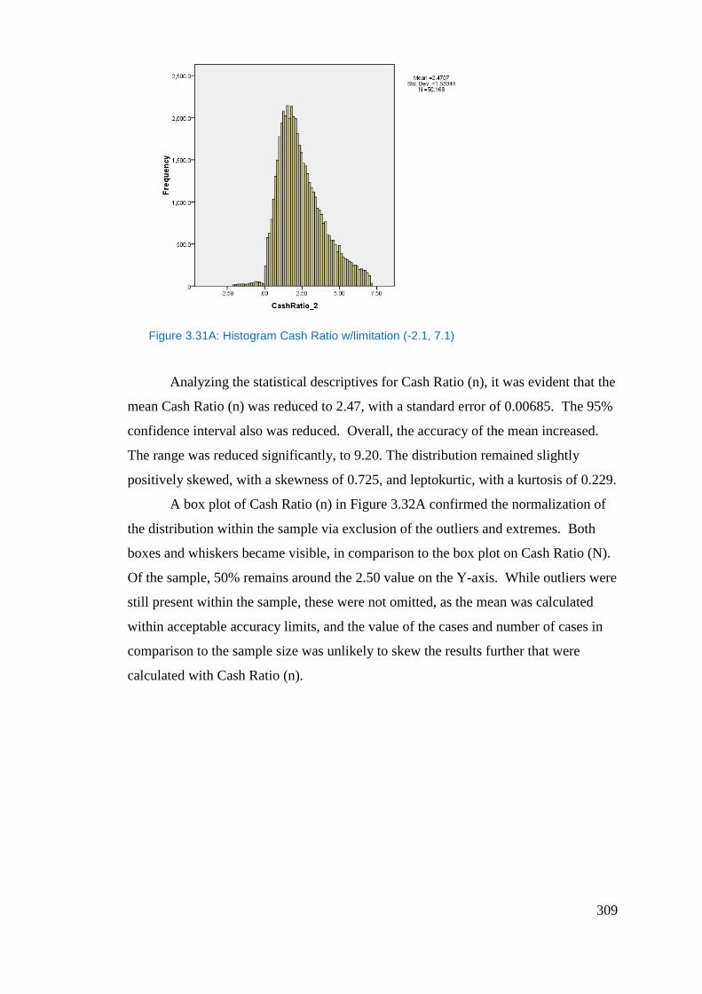
309
Figure 3.31A: Histogram Cash Ratio w/limitation (-2.1, 7.1)
Analyzing the statistical descriptives for Cash Ratio (n), it was evident that the
mean Cash Ratio (n) was reduced to 2.47, with a standard error of 0.00685. The 95%
confidence interval also was reduced. Overall, the accuracy of the mean increased.
The range was reduced significantly, to 9.20. The distribution remained slightly
positively skewed, with a skewness of 0.725, and leptokurtic, with a kurtosis of 0.229.
A box plot of Cash Ratio (n) in Figure 3.32A confirmed the normalization of
the distribution within the sample via exclusion of the outliers and extremes. Both
boxes and whiskers became visible, in comparison to the box plot on Cash Ratio (N).
Of the sample, 50% remains around the 2.50 value on the Y-axis. While outliers were
still present within the sample, these were not omitted, as the mean was calculated
within acceptable accuracy limits, and the value of the cases and number of cases in
comparison to the sample size was unlikely to skew the results further that were
calculated with Cash Ratio (n).
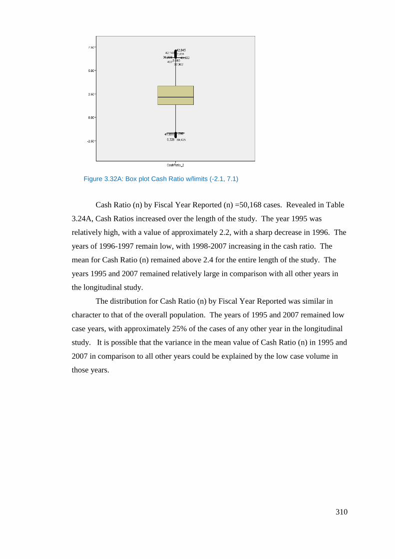
310
Figure 3.32A: Box plot Cash Ratio w/limits (-2.1, 7.1)
Cash Ratio (n) by Fiscal Year Reported (n) =50,168 cases. Revealed in Table
3.24A, Cash Ratios increased over the length of the study. The year 1995 was
relatively high, with a value of approximately 2.2, with a sharp decrease in 1996. The
years of 1996-1997 remain low, with 1998-2007 increasing in the cash ratio. The
mean for Cash Ratio (n) remained above 2.4 for the entire length of the study. The
years 1995 and 2007 remained relatively large in comparison with all other years in
the longitudinal study.
The distribution for Cash Ratio (n) by Fiscal Year Reported was similar in
character to that of the overall population. The years of 1995 and 2007 remained low
case years, with approximately 25% of the cases of any other year in the longitudinal
study. It is possible that the variance in the mean value of Cash Ratio (n) in 1995 and
2007 in comparison to all other years could be explained by the low case volume in
those years.
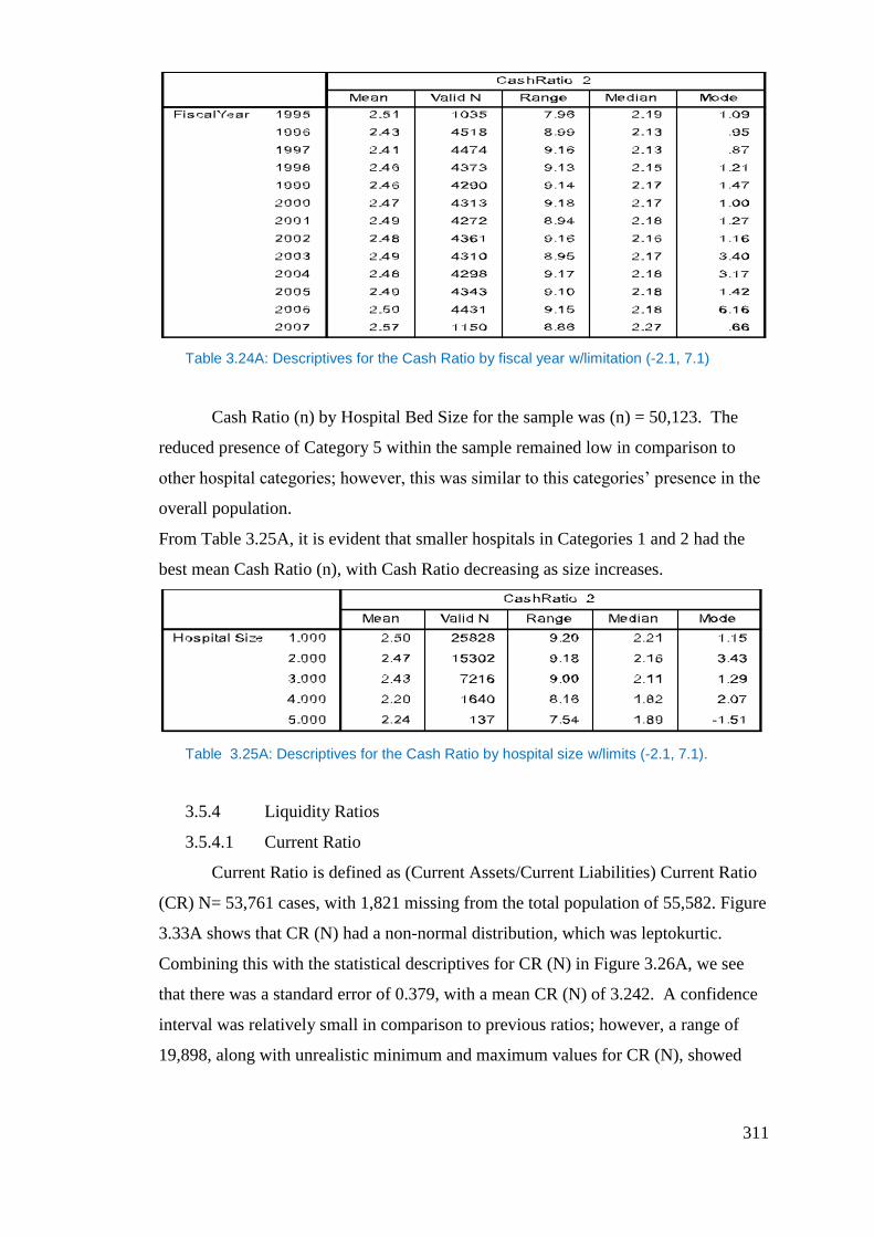
311
Table 3.24A: Descriptives for the Cash Ratio by fiscal year w/limitation (-2.1, 7.1)
Cash Ratio (n) by Hospital Bed Size for the sample was (n) = 50,123. The
reduced presence of Category 5 within the sample remained low in comparison to
other hospital categories; however, this was similar to this categories’ presence in the
overall population.
From Table 3.25A, it is evident that smaller hospitals in Categories 1 and 2 had the
best mean Cash Ratio (n), with Cash Ratio decreasing as size increases.
Table 3.25A: Descriptives for the Cash Ratio by hospital size w/limits (-2.1, 7.1).
3.5.4 Liquidity Ratios
3.5.4.1 Current Ratio
Current Ratio is defined as (Current Assets/Current Liabilities) Current Ratio
(CR) N= 53,761 cases, with 1,821 missing from the total population of 55,582. Figure
3.33A shows that CR (N) had a non-normal distribution, which was leptokurtic.
Combining this with the statistical descriptives for CR (N) in Figure 3.26A, we see
that there was a standard error of 0.379, with a mean CR (N) of 3.242. A confidence
interval was relatively small in comparison to previous ratios; however, a range of
19,898, along with unrealistic minimum and maximum values for CR (N), showed
312
that outliers and extremes were present and were distorting the mean. The
distribution was skewed positively, with a skewness of 83.43, and leptokurtic was
confirmed, with a kurtosis value of 13,976.81.
Figure 3.33A: Histogram Current Ratio with no limitations
The box plot in Figure 3.34A confirmed a non-normal distribution, with no
boxes or whiskers visible. Outliers and extremes were identified as extending above
and below the line present at the 0 mark, which represents 50% of the total
population.
Figure 3.34A: Box plot Current Ratio with no limitations
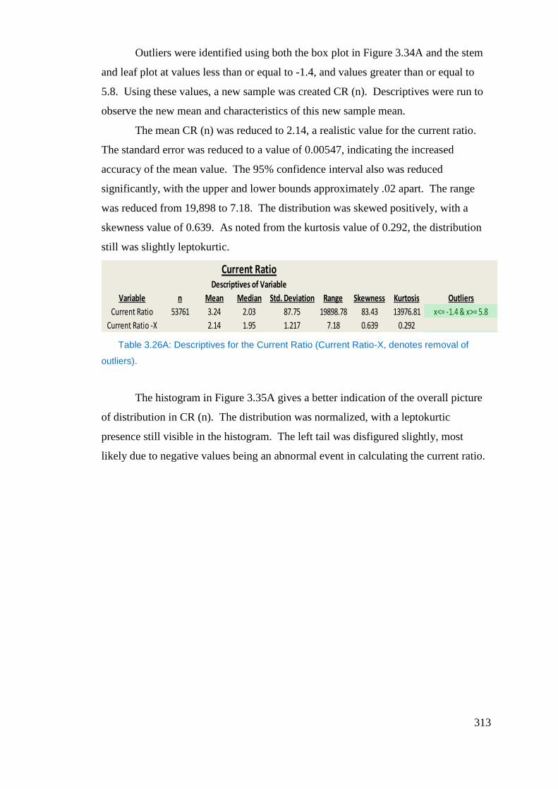
313
Outliers were identified using both the box plot in Figure 3.34A and the stem
and leaf plot at values less than or equal to -1.4, and values greater than or equal to
5.8. Using these values, a new sample was created CR (n). Descriptives were run to
observe the new mean and characteristics of this new sample mean.
The mean CR (n) was reduced to 2.14, a realistic value for the current ratio.
The standard error was reduced to a value of 0.00547, indicating the increased
accuracy of the mean value. The 95% confidence interval also was reduced
significantly, with the upper and lower bounds approximately .02 apart. The range
was reduced from 19,898 to 7.18. The distribution was skewed positively, with a
skewness value of 0.639. As noted from the kurtosis value of 0.292, the distribution
still was slightly leptokurtic.
Table 3.26A: Descriptives for the Current Ratio (Current Ratio-X, denotes removal of
outliers).
The histogram in Figure 3.35A gives a better indication of the overall picture
of distribution in CR (n). The distribution was normalized, with a leptokurtic
presence still visible in the histogram. The left tail was disfigured slightly, most
likely due to negative values being an abnormal event in calculating the current ratio.
Current RatioDescriptives of Variable
Variable n Mean Median Std. Deviation Range Skewness Kurtosis Outliers
Current Ratio 53761 3.24 2.03 87.75 19898.78 83.43 13976.81 x<= -1.4 & x>= 5.8
Current Ratio -X 2.14 1.95 1.217 7.18 0.639 0.292
314
Figure 3.35A: Histogram Current Ratio with Limitation (-1.4, 5.8)
The box plot in Figure 3.36A confirmed normalization of the data, with boxes
and whiskers fully visible. It was noted that the lower whisker extends below the zero
value, indicating that more than outliers and extremes were present below zero.
Outliers were still visible in the box plot; however, these should not affect further
research using this sample, due to the values of the CR or the number of outliers
present in comparison to the overall CR (n) case count. Standard error confirmed
accuracy in the mean CR (n) as well.
Figure 0.1.36A: Box plot of Current Ratio w/limitations (-1.4, 5.8)
Analyzing the mean CR (n) by Fiscal Year Reported in Table 3.27A (n
=49,524), the mean was reduced from the year 1995 with a value of 2.20, finishing in
2007 with a value of 2.12. While there was not a complete linear decline, the overall
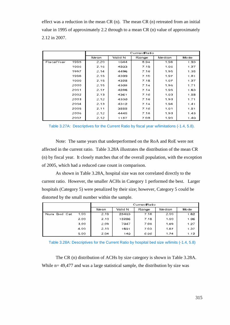
315
effect was a reduction in the mean CR (n). The mean CR (n) retreated from an initial
value in 1995 of approximately 2.2 through to a mean CR (n) value of approximately
2.12 in 2007.
Table 3.27A: Descriptives for the Current Ratio by fiscal year w/limitations (-1.4, 5.8).
Note: The same years that underperformed on the RoA and RoE were not
affected in the current ratio. Table 3.28A illustrates the distribution of the mean CR
(n) by fiscal year. It closely matches that of the overall population, with the exception
of 2005, which had a reduced case count in comparison.
As shown in Table 3.28A, hospital size was not correlated directly to the
current ratio. However, the smaller ACHs in Category 1 performed the best. Larger
hospitals (Category 5) were penalized by their size; however, Category 5 could be
distorted by the small number within the sample.
Table 3.28A: Descriptives for the Current Ratio by hospital bed size w/limits (-1.4, 5.8)
The CR (n) distribution of ACHs by size category is shown in Table 3.28A.
While n= 49,477 and was a large statistical sample, the distribution by size was
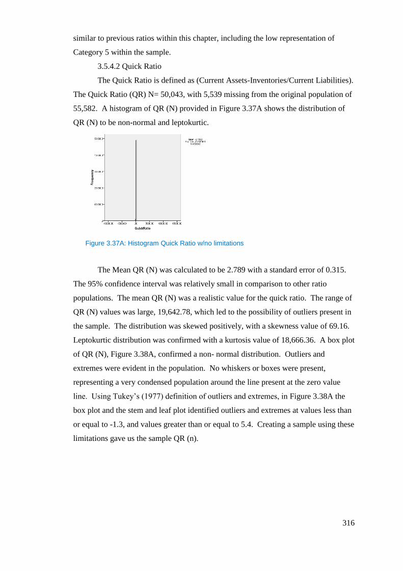
316
similar to previous ratios within this chapter, including the low representation of
Category 5 within the sample.
3.5.4.2 Quick Ratio
The Quick Ratio is defined as (Current Assets-Inventories/Current Liabilities).
The Quick Ratio (QR) N= 50,043, with 5,539 missing from the original population of
55,582. A histogram of QR (N) provided in Figure 3.37A shows the distribution of
QR (N) to be non-normal and leptokurtic.
Figure 3.37A: Histogram Quick Ratio w/no limitations
The Mean QR (N) was calculated to be 2.789 with a standard error of 0.315.
The 95% confidence interval was relatively small in comparison to other ratio
populations. The mean QR (N) was a realistic value for the quick ratio. The range of
QR (N) values was large, 19,642.78, which led to the possibility of outliers present in
the sample. The distribution was skewed positively, with a skewness value of 69.16.
Leptokurtic distribution was confirmed with a kurtosis value of 18,666.36. A box plot
of QR (N), Figure 3.38A, confirmed a non- normal distribution. Outliers and
extremes were evident in the population. No whiskers or boxes were present,
representing a very condensed population around the line present at the zero value
line. Using Tukey’s (1977) definition of outliers and extremes, in Figure 3.38A the
box plot and the stem and leaf plot identified outliers and extremes at values less than
or equal to -1.3, and values greater than or equal to 5.4. Creating a sample using these
limitations gave us the sample QR (n).
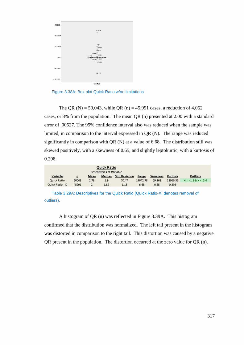
317
Figure 3.38A: Box plot Quick Ratio w/no limitations
The QR (N) = 50,043, while QR (n) = 45,991 cases, a reduction of 4,052
cases, or 8% from the population. The mean QR (n) presented at 2.00 with a standard
error of .00527. The 95% confidence interval also was reduced when the sample was
limited, in comparison to the interval expressed in QR (N). The range was reduced
significantly in comparison with QR (N) at a value of 6.68. The distribution still was
skewed positively, with a skewness of 0.65, and slightly leptokurtic, with a kurtosis of
0.298.
Table 3.29A: Descriptives for the Quick Ratio (Quick Ratio-X, denotes removal of
outliers).
A histogram of QR (n) was reflected in Figure 3.39A. This histogram
confirmed that the distribution was normalized. The left tail present in the histogram
was distorted in comparison to the right tail. This distortion was caused by a negative
QR present in the population. The distortion occurred at the zero value for QR (n).
Quick RatioDescriptives of Variable
Variable n Mean Median Std. Deviation Range Skewness Kurtosis Outliers
Quick Ratio 50043 2.78 1.9 70.47 19642.78 69.163 18666.36 X<= -1.3 & X>= 5.4
Quick Ratio - X 45991 2 1.82 1.13 6.68 0.65 0.298
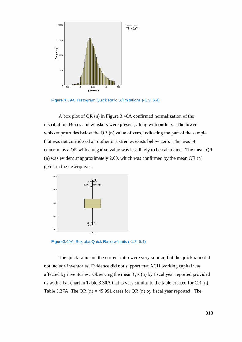
318
Figure 3.39A: Histogram Quick Ratio w/limitations (-1.3, 5.4)
A box plot of QR (n) in Figure 3.40A confirmed normalization of the
distribution. Boxes and whiskers were present, along with outliers. The lower
whisker protrudes below the QR (n) value of zero, indicating the part of the sample
that was not considered an outlier or extremes exists below zero. This was of
concern, as a QR with a negative value was less likely to be calculated. The mean QR
(n) was evident at approximately 2.00, which was confirmed by the mean QR (n)
given in the descriptives.
Figure3.40A: Box plot Quick Ratio w/limits (-1.3, 5.4)
The quick ratio and the current ratio were very similar, but the quick ratio did
not include inventories. Evidence did not support that ACH working capital was
affected by inventories. Observing the mean QR (n) by fiscal year reported provided
us with a bar chart in Table 3.30A that is very similar to the table created for CR (n),
Table 3.27A. The QR (n) = 45,991 cases for QR (n) by fiscal year reported. The
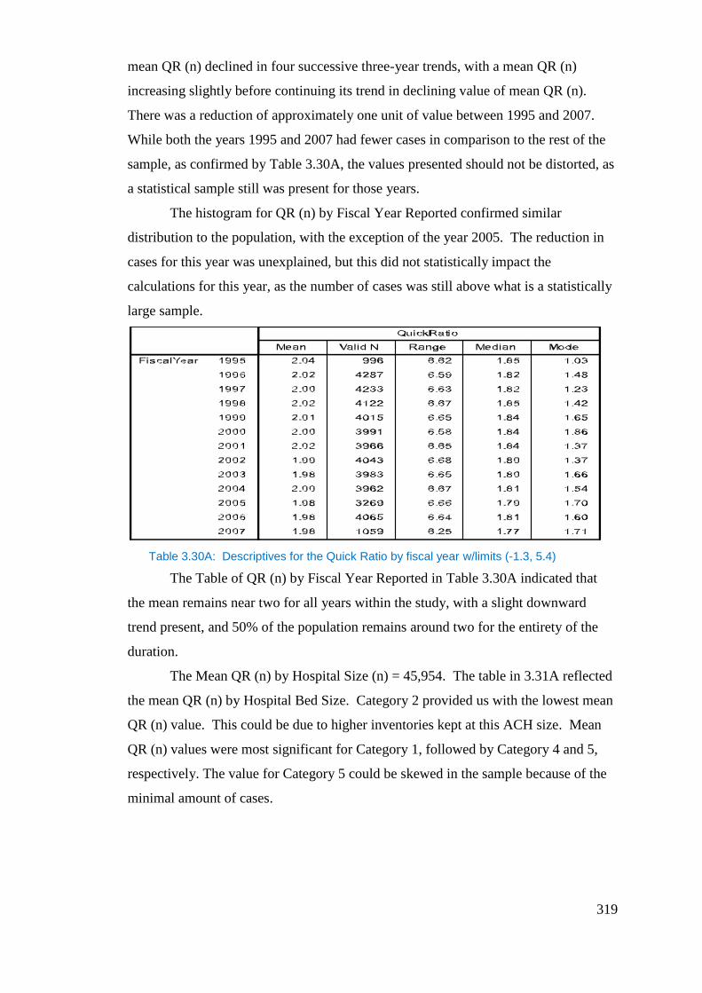
319
mean QR (n) declined in four successive three-year trends, with a mean QR (n)
increasing slightly before continuing its trend in declining value of mean QR (n).
There was a reduction of approximately one unit of value between 1995 and 2007.
While both the years 1995 and 2007 had fewer cases in comparison to the rest of the
sample, as confirmed by Table 3.30A, the values presented should not be distorted, as
a statistical sample still was present for those years.
The histogram for QR (n) by Fiscal Year Reported confirmed similar
distribution to the population, with the exception of the year 2005. The reduction in
cases for this year was unexplained, but this did not statistically impact the
calculations for this year, as the number of cases was still above what is a statistically
large sample.
Table 3.30A: Descriptives for the Quick Ratio by fiscal year w/limits (-1.3, 5.4)
The Table of QR (n) by Fiscal Year Reported in Table 3.30A indicated that
the mean remains near two for all years within the study, with a slight downward
trend present, and 50% of the population remains around two for the entirety of the
duration.
The Mean QR (n) by Hospital Size (n) = 45,954. The table in 3.31A reflected
the mean QR (n) by Hospital Bed Size. Category 2 provided us with the lowest mean
QR (n) value. This could be due to higher inventories kept at this ACH size. Mean
QR (n) values were most significant for Category 1, followed by Category 4 and 5,
respectively. The value for Category 5 could be skewed in the sample because of the
minimal amount of cases.
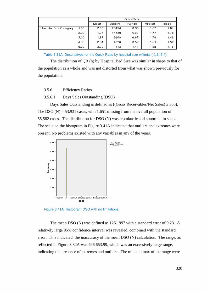
320
Table 3.31A: Descriptives for the Quick Ratio by hospital size w/limits (-1.3, 5.4)
The distribution of QR (n) by Hospital Bed Size was similar in shape to that of
the population as a whole and was not distorted from what was shown previously for
the population.
3.5.6 Efficiency Ratios
3.5.6.1 Days Sales Outstanding (DSO)
Days Sales Outstanding is defined as ((Gross Receivables/Net Sales) x 365).
The DSO (N) = 53,931 cases, with 1,651 missing from the overall population of
55,582 cases. The distribution for DSO (N) was leptokurtic and abnormal in shape.
The scale on the histogram in Figure 3.41A indicated that outliers and extremes were
present. No problems existed with any variables in any of the years.
Figure 3.41A: Histogram DSO with no limitations
The mean DSO (N) was defined as 126.1997 with a standard error of 9.23. A
relatively large 95% confidence interval was revealed, combined with the standard
error. This indicated the inaccuracy of the mean DSO (N) calculation. The range, as
reflected in Figure 3.32A was 496,653.99, which was an excessively large range,
indicating the presence of extremes and outliers. The min and max of the range were
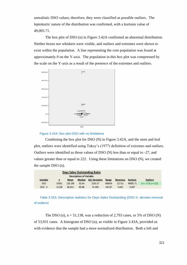
321
unrealistic DSO values; therefore, they were classified as possible outliers. The
leptokurtic nature of the distribution was confirmed, with a kurtosis value of
49,005.71.
The box plot of DSO (n) in Figure 3.42A confirmed an abnormal distribution.
Neither boxes nor whiskers were visible, and outliers and extremes were shown to
exist within the population. A line representing the core population was found at
approximately 0 on the Y-axis. The population in this box plot was compressed by
the scale on the Y-axis as a result of the presence of the extremes and outliers.
Figure 3.42A: Box plot DSO with no limitations
Combining the box plot for DSO (N) in Figure 3.42A, and the stem and leaf
plot, outliers were identified using Tukey’s (1977) definition of extremes and outliers.
Outliers were identified as those values of DSO (N) less than or equal to -27, and
values greater than or equal to 222. Using these limitations on DSO (N), we created
the sample DSO (n).
Table 3.32A: Descriptive statistics for Days Sales Outstanding (DSO-X, denotes removal
of outliers)
The DSO (n), n = 51,138, was a reduction of 2,793 cases, or 5% of DSO (N)
of 53,931 cases. A histogram of DSO (n), as visible in Figure 3.43A, provided us
with evidence that the sample had a more normalized distribution. Both a left and
Days Sales Outstanding RatioDescriptives of Variable
Variable n Mean Median Std. Deviation Range Skewness Kurtosis Outliers
DSO 53931 126.199 92.64 2143.57 496654 217.61 49005.71 x<= -27 & x>=222
DSO - X 51138 96.813 89.88 41.905 245.87 0.655 0.097
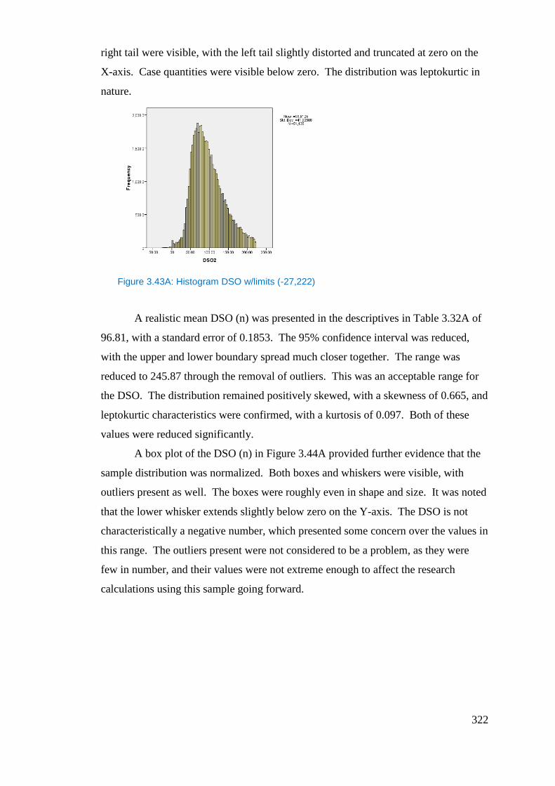
322
right tail were visible, with the left tail slightly distorted and truncated at zero on the
X-axis. Case quantities were visible below zero. The distribution was leptokurtic in
nature.
Figure 3.43A: Histogram DSO w/limits (-27,222)
A realistic mean DSO (n) was presented in the descriptives in Table 3.32A of
96.81, with a standard error of 0.1853. The 95% confidence interval was reduced,
with the upper and lower boundary spread much closer together. The range was
reduced to 245.87 through the removal of outliers. This was an acceptable range for
the DSO. The distribution remained positively skewed, with a skewness of 0.665, and
leptokurtic characteristics were confirmed, with a kurtosis of 0.097. Both of these
values were reduced significantly.
A box plot of the DSO (n) in Figure 3.44A provided further evidence that the
sample distribution was normalized. Both boxes and whiskers were visible, with
outliers present as well. The boxes were roughly even in shape and size. It was noted
that the lower whisker extends slightly below zero on the Y-axis. The DSO is not
characteristically a negative number, which presented some concern over the values in
this range. The outliers present were not considered to be a problem, as they were
few in number, and their values were not extreme enough to affect the research
calculations using this sample going forward.
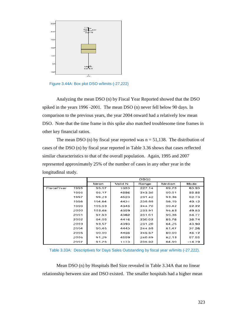
323
Figure 3.44A: Box plot DSO w/limits (-27,222)
Analyzing the mean DSO (n) by Fiscal Year Reported showed that the DSO
spiked in the years 1996 -2001. The mean DSO (n) never fell below 90 days. In
comparison to the previous years, the year 2004 onward had a relatively low mean
DSO. Note that the time frame in this spike also matched troublesome time frames in
other key financial ratios.
The mean DSO (n) by fiscal year reported was n = 51,138. The distribution of
cases of the DSO (n) by fiscal year reported in Table 3.36 shows that cases reflected
similar characteristics to that of the overall population. Again, 1995 and 2007
represented approximately 25% of the number of cases in any other year in the
longitudinal study.
Table 3.33A: Descriptives for Days Sales Outstanding by fiscal year w/limits (-27,222).
Mean DSO (n) by Hospitals Bed Size revealed in Table 3.34A that no linear
relationship between size and DSO existed. The smaller hospitals had a higher mean
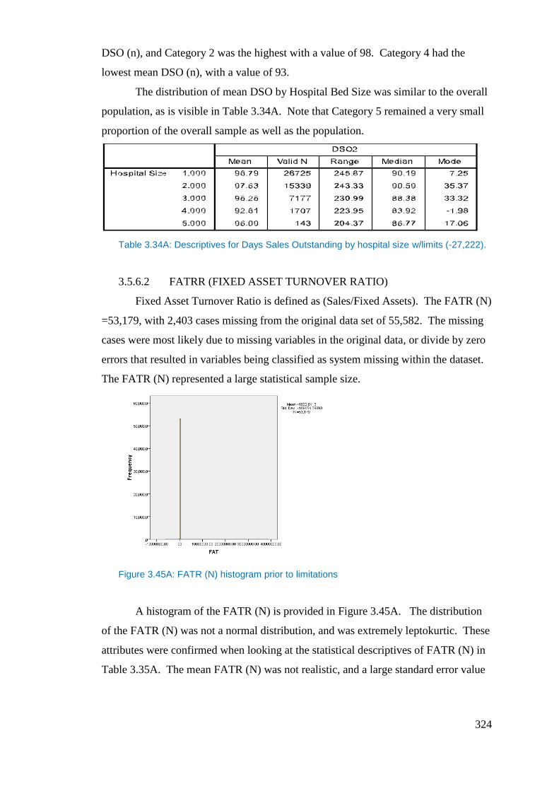
324
DSO (n), and Category 2 was the highest with a value of 98. Category 4 had the
lowest mean DSO (n), with a value of 93.
The distribution of mean DSO by Hospital Bed Size was similar to the overall
population, as is visible in Table 3.34A. Note that Category 5 remained a very small
proportion of the overall sample as well as the population.
Table 3.34A: Descriptives for Days Sales Outstanding by hospital size w/limits (-27,222).
3.5.6.2 FATRR (FIXED ASSET TURNOVER RATIO)
Fixed Asset Turnover Ratio is defined as (Sales/Fixed Assets). The FATR (N)
=53,179, with 2,403 cases missing from the original data set of 55,582. The missing
cases were most likely due to missing variables in the original data, or divide by zero
errors that resulted in variables being classified as system missing within the dataset.
The FATR (N) represented a large statistical sample size.
Figure 3.45A: FATR (N) histogram prior to limitations
A histogram of the FATR (N) is provided in Figure 3.45A. The distribution
of the FATR (N) was not a normal distribution, and was extremely leptokurtic. These
attributes were confirmed when looking at the statistical descriptives of FATR (N) in
Table 3.35A. The mean FATR (N) was not realistic, and a large standard error value
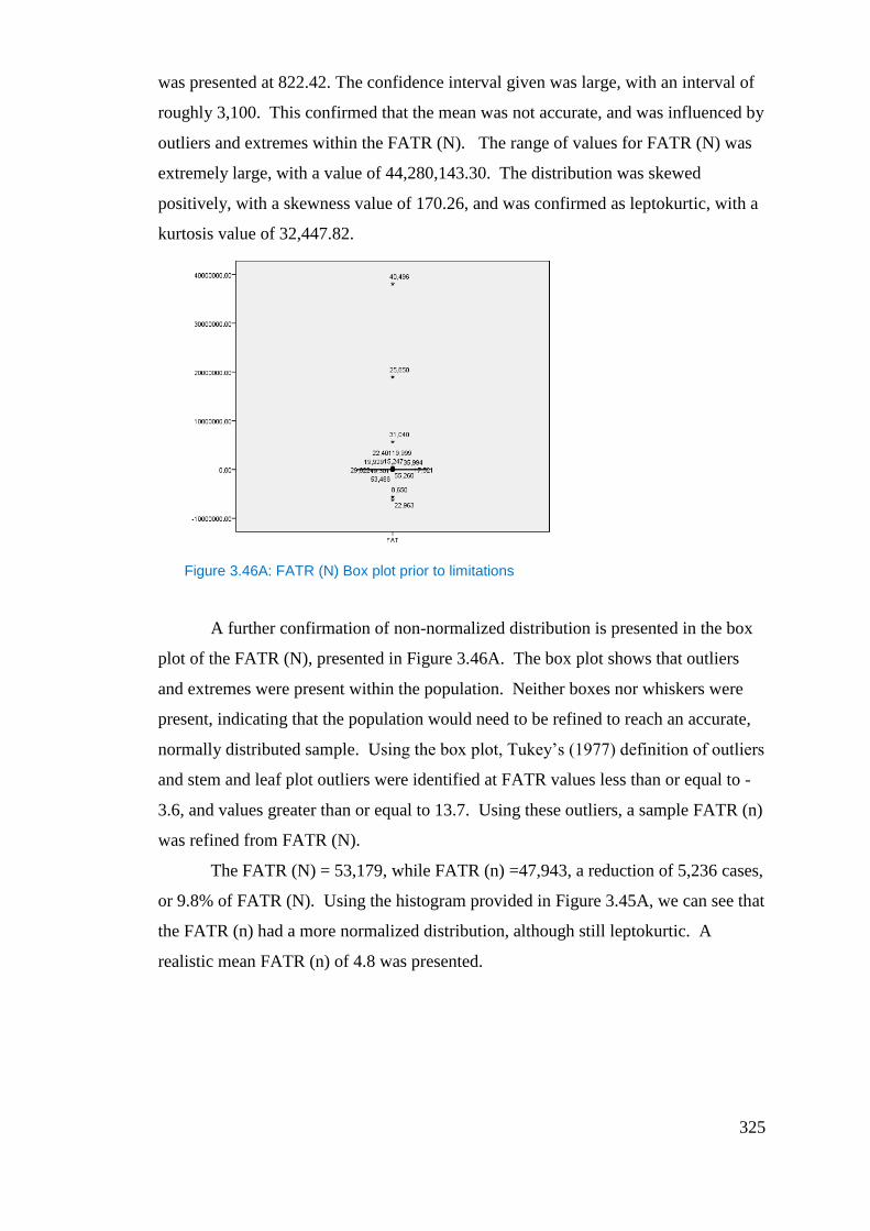
325
was presented at 822.42. The confidence interval given was large, with an interval of
roughly 3,100. This confirmed that the mean was not accurate, and was influenced by
outliers and extremes within the FATR (N). The range of values for FATR (N) was
extremely large, with a value of 44,280,143.30. The distribution was skewed
positively, with a skewness value of 170.26, and was confirmed as leptokurtic, with a
kurtosis value of 32,447.82.
Figure 3.46A: FATR (N) Box plot prior to limitations
A further confirmation of non-normalized distribution is presented in the box
plot of the FATR (N), presented in Figure 3.46A. The box plot shows that outliers
and extremes were present within the population. Neither boxes nor whiskers were
present, indicating that the population would need to be refined to reach an accurate,
normally distributed sample. Using the box plot, Tukey’s (1977) definition of outliers
and stem and leaf plot outliers were identified at FATR values less than or equal to -
3.6, and values greater than or equal to 13.7. Using these outliers, a sample FATR (n)
was refined from FATR (N).
The FATR (N) = 53,179, while FATR (n) =47,943, a reduction of 5,236 cases,
or 9.8% of FATR (N). Using the histogram provided in Figure 3.45A, we can see that
the FATR (n) had a more normalized distribution, although still leptokurtic. A
realistic mean FATR (n) of 4.8 was presented.
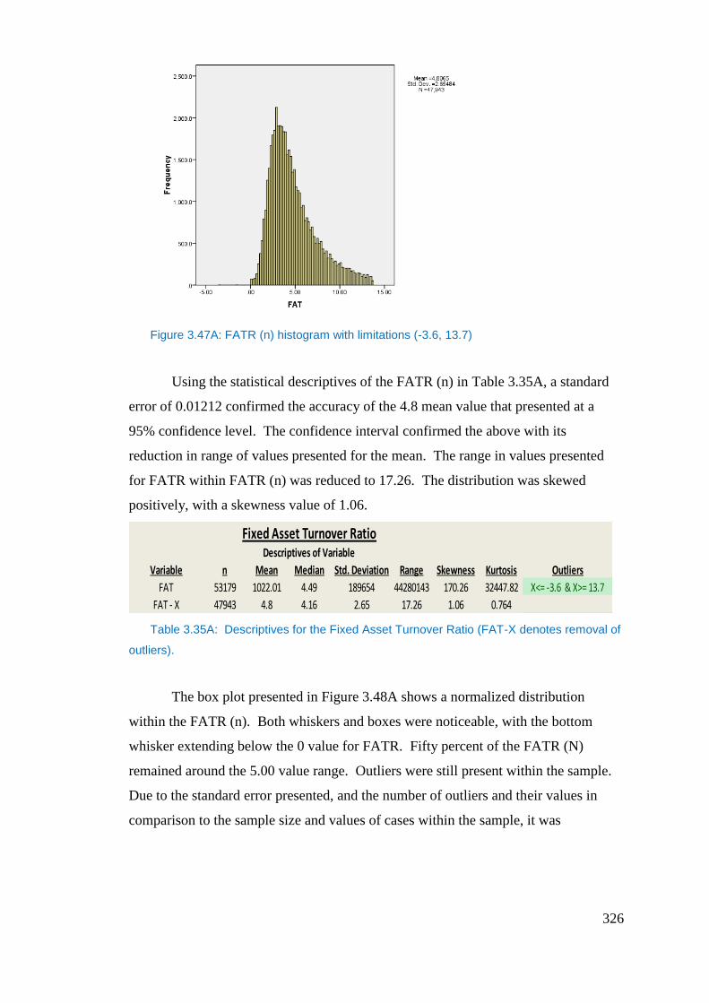
326
Figure 3.47A: FATR (n) histogram with limitations (-3.6, 13.7)
Using the statistical descriptives of the FATR (n) in Table 3.35A, a standard
error of 0.01212 confirmed the accuracy of the 4.8 mean value that presented at a
95% confidence level. The confidence interval confirmed the above with its
reduction in range of values presented for the mean. The range in values presented
for FATR within FATR (n) was reduced to 17.26. The distribution was skewed
positively, with a skewness value of 1.06.
Table 3.35A: Descriptives for the Fixed Asset Turnover Ratio (FAT-X denotes removal of
outliers).
The box plot presented in Figure 3.48A shows a normalized distribution
within the FATR (n). Both whiskers and boxes were noticeable, with the bottom
whisker extending below the 0 value for FATR. Fifty percent of the FATR (N)
remained around the 5.00 value range. Outliers were still present within the sample.
Due to the standard error presented, and the number of outliers and their values in
comparison to the sample size and values of cases within the sample, it was
Fixed Asset Turnover RatioDescriptives of Variable
Variable n Mean Median Std. Deviation Range Skewness Kurtosis Outliers
FAT 53179 1022.01 4.49 189654 44280143 170.26 32447.82 X<= -3.6 & X>= 13.7
FAT - X 47943 4.8 4.16 2.65 17.26 1.06 0.764
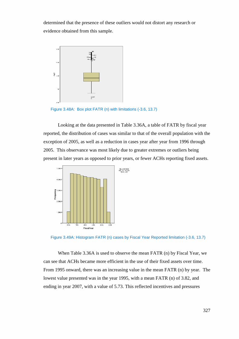
327
determined that the presence of these outliers would not distort any research or
evidence obtained from this sample.
Figure 3.48A: Box plot FATR (n) with limitations (-3.6, 13.7)
Looking at the data presented in Table 3.36A, a table of FATR by fiscal year
reported, the distribution of cases was similar to that of the overall population with the
exception of 2005, as well as a reduction in cases year after year from 1996 through
2005. This observance was most likely due to greater extremes or outliers being
present in later years as opposed to prior years, or fewer ACHs reporting fixed assets.
Figure 3.49A: Histogram FATR (n) cases by Fiscal Year Reported limitation (-3.6, 13.7)
When Table 3.36A is used to observe the mean FATR (n) by Fiscal Year, we
can see that ACHs became more efficient in the use of their fixed assets over time.
From 1995 onward, there was an increasing value in the mean FATR (n) by year. The
lowest value presented was in the year 1995, with a mean FATR (n) of 3.82, and
ending in year 2007, with a value of 5.73. This reflected incentives and pressures
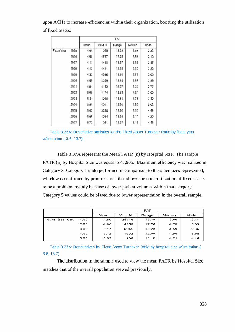
328
upon ACHs to increase efficiencies within their organization, boosting the utilization
of fixed assets.
Table 3.36A: Descriptive statistics for the Fixed Asset Turnover Ratio by fiscal year
w/limitation (-3.6, 13.7)
Table 3.37A represents the Mean FATR (n) by Hospital Size. The sample
FATR (n) by Hospital Size was equal to 47,905. Maximum efficiency was realized in
Category 3. Category 1 underperformed in comparison to the other sizes represented,
which was confirmed by prior research that shows the underutilization of fixed assets
to be a problem, mainly because of lower patient volumes within that category.
Category 5 values could be biased due to lower representation in the overall sample.
Table 3.37A: Descriptives for Fixed Asset Turnover Ratio by hospital size w/limitation (-
3.6, 13.7)
The distribution in the sample used to view the mean FATR by Hospital Size
matches that of the overall population viewed previously.

329
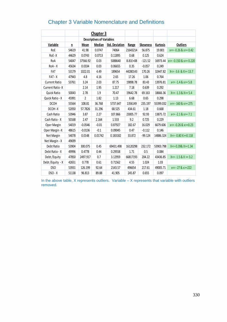
330
Chapter 3 Variable Nomenclature and Definitions
In the above table, X represents outliers. Variable – X represents that variable with outliers removed.
Chapter 3Descriptives of Variables
Variable n Mean Median Std. Deviation Range Skewness Kurtosis Outliers
RoE 54619 41.98 0.0747 74064 21643214 56.875 19.801 x<= -0.26 & x>= 0.42
RoE -X 44629 0.0743 0.0713 0.11895 0.68 0.125 0.624
RoA 54047 37566.92 0.03 5088640 8.81E+08 -121.52 16973.44 x<= -0.150 & x>= 0.220
RoA - X 45634 0.0334 0.03 0.06655 0.35 -0.057 0.249
FAT 53179 1022.01 4.49 189654 44280143 170.26 32447.82 X<= -3.6 & X>= 13.7
FAT - X 47943 4.8 4.16 2.65 17.26 1.06 0.764
Current Ratio 53761 3.24 2.03 87.75 19898.78 83.43 13976.81 x<= -1.4 & x>= 5.8
Current Ratio -X 2.14 1.95 1.217 7.18 0.639 0.292
Quick Ratio 50043 2.78 1.9 70.47 19642.78 69.163 18666.36 X<= -1.3 & X>= 5.4
Quick Ratio - X 45991 2 1.82 1.13 6.68 0.65 0.298
DCOH 55564 108.81 36.768 5737.647 1356149 235.197 55399.032 x<= -160 & x>= 275
DCOH -X 52050 57.7826 31.296 68.525 434.61 1.18 0.668
Cash Ratio 53946 3.87 2.27 107.866 23005.77 92.93 13875.72 x<= -2.1 & x>= 7.1
Cash Ratio - X 50168 2.47 2.164 1.533 9.2 0.725 0.229
Oper Margin 54019 -0.0546 -0.01 0.87927 182.67 16.029 6679.606 x<= -0.26 & x>=0.23
Oper Margin -X 48615 -0.0136 -0.1 0.09045 0.47 -0.112 0.146
Net Margin 54078 0.0148 0.01742 0.183182 33.872 -99.124 14886.324 X<= -0.80 X>=0.118
Net Margin - X 49699
Debt Ratio 53904 300.075 0.45 69431.498 16120298 232.172 53903.798 X<=-0.39& X>=1.34
Debt Ratio - X 49996 0.4778 0.44 0.29558 1.71 0.5 0.084
Debt /Equity 47850 2497.917 0.7 3.12959 66817193 204.22 43436.85 X<= -1.5 & X >= 3.2
Debt /Equity - X 42651 0.778 0.61 0.71562 4.55 1.024 1.03
DSO 53931 126.199 92.64 2143.57 496654 217.61 49005.71 x<= -27 & x>=222
DSO - X 51138 96.813 89.88 41.905 245.87 0.655 0.097

331
Chapter 4 Variable Nomenclature and Definitions
Variable Variable Nomenclature Provided Calculated Outliers Definitionhospital size Num_Bed X Hospital size denoted by number of beds
hospital size Hospital Size X Hospital size catergorized by the number of beds ( 5 categories)
Percent Government Business % Gov_Bus X X<=0.25 (TitleXVII +Title XIX)patient days/ (total In/Outpatient Days)
Debt to Equity Ratio D/E X X<= -1.5&X>=3.2 Total Debt /Equity
Cash Position cash position X Total Cash/Total Assets
Leverage Leverage X X<= -0.37 & X>=0.96 Total Longterm Liabilities/Total Assets
Leverage 2 Leverage_2 X X >= 0.99 Leverage ( non-negative value)
Current Ratio Current Ratio X x<= -1.4 & x>= 5.8 Current Assets/Current Liabilities
Quick Ratio Quick Ratio X X<= -1.3 & X>= 5.4 (Current Assets- Inventories)/ Current Liabilities
Liquidity Liquidity X X<= -0.11 & X >=0.79 Current Assets/ Total Assets
Debt Ratio debt_ratio X X<=-0.39& X>=1.34 Total Liabilities/ Total Assets
Debt Ratio 2 debt_ratio_2 X X >= 1.34 Debt Ratio (non- negative values)
Total Assets TA X
Natural Log Total Assets LnTA X natural log of Total Assets
fiscal year Fiscal Year X Fiscal Year
Net Margin net_marg X X<= -0.80 X>=0.118 Net Income/ Sales
Capital Cost Proxy CCProxy X Total Interest Expense/ Total Liabilities
Operating Cash Flows OCF X X<= -27,995,730 & X > 40,069,436 FCF + CAPEX
Free Cash Flows FCF X X<= -32,186,314 & X > 36,290,518 net income+(amortization,depreciation)-delta working capital- capex
Change in Free Cash Flows Delta_FCF x X<=-70227629 & X>=63609001 FCF - Prev_Yr_FCF
% Change in Free Cash Flows %_Delta_FCF x X<=-5.1 & X>=2.3 (FCF - Prev_Yr_FCF)/Prev_Yr_FCF
Capital Expenditures CAPEX X X <= 0 & X >= 38209778
Capital Expenditures 2 CAPEX 2 X X<= 0 & X >= 12,375,048 CAPEX (non- negative values)
Change in Fixed Assets Delta FA X X<= -23 & X>= 27 FA- Prev_Yr_FA
Change in Fixed Assets 2 Delta FA2 X X<= 0 & X>= 27 Delta FA (non-negative values)
Depreciation Depreciation X Depreciation
Depreciation 2 X X>=9509812 Depreciation (non-negative values)
RoE RoE2 X x<= -0.26 & x>=0.42 Net Income/ Shareholders Equity
RoA RoA X x<= -0.150 & x>=0.220 Net Income/ Total Assets
FAT FAT X X<= -3.6 & X>= 13.7 Sales / Fixed Assets
Days Cash on Hand Days Cash on Hand 3 X x<= -160 & x>=275 (Cash on Hand+investments+temp investments)/ operating expenses/365
Working Capital X current assets - current liabilities
Cash Ratio CashRatio_2 X x<= -2.1 &x>=7.1 (cash equilvilents+temp investments+AR)/ Current Liabilities
Operating Income Margin OperatingIncomeMargin X x<= -0.26 & x>=0.23 operating income/ net sales
Cash Turnover Cash Turnover X Net Sales/ Cash
Total Asset Turnover TA_turnover X Net Sales/Avg Total Assets
DSO DSO2 X x<= -27 & x>=222 Gross Recievables/ net sales/365
X denotes outliers beyond three standard deviations.
Note: Not all ratios listed were used in the final study… Some ratios were removed due to reduced sample size due to missing values or could not be computed due to lack of information.
They are listed to better understand the scope of research performed.
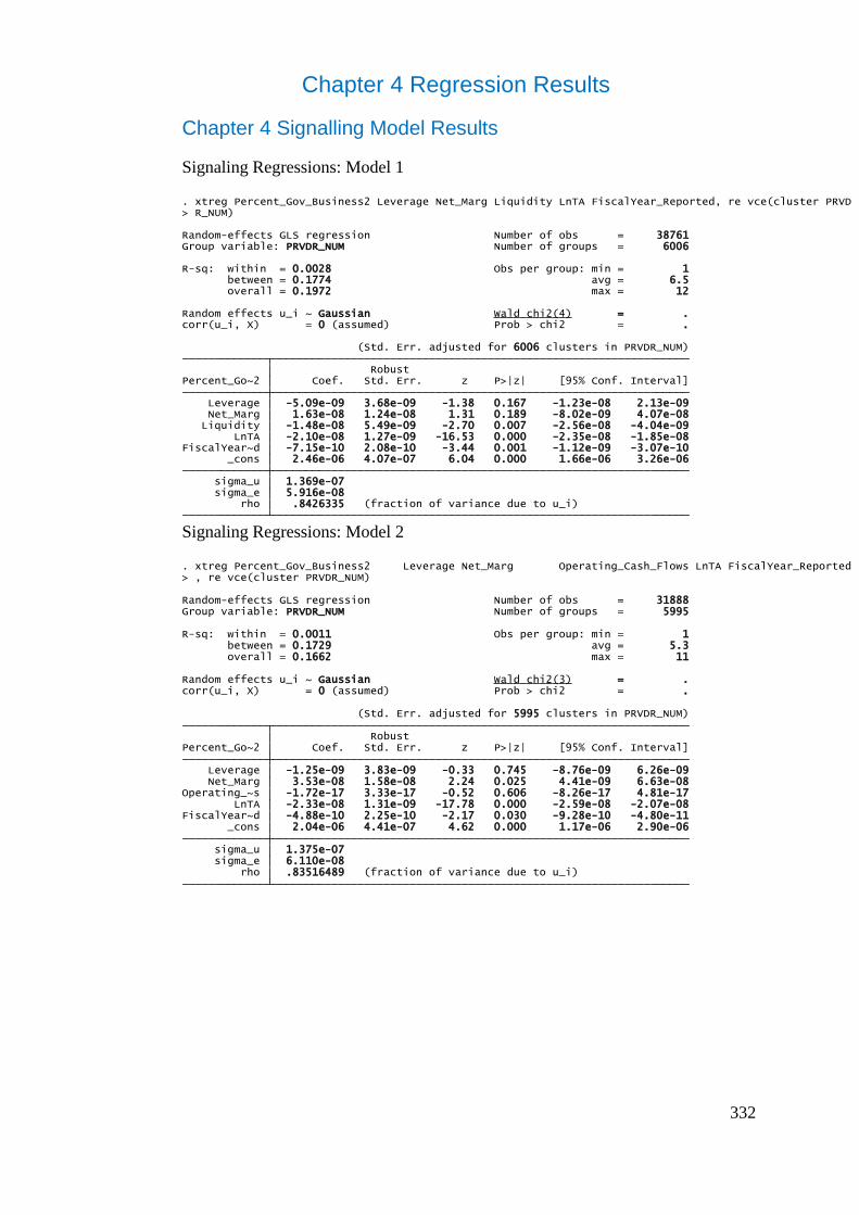
332
Chapter 4 Regression Results
Chapter 4 Signalling Model Results
Signaling Regressions: Model 1
Signaling Regressions: Model 2
rho .8426335 (fraction of variance due to u_i) sigma_e 5.916e-08 sigma_u 1.369e-07 _cons 2.46e-06 4.07e-07 6.04 0.000 1.66e-06 3.26e-06FiscalYear~d -7.15e-10 2.08e-10 -3.44 0.001 -1.12e-09 -3.07e-10 LnTA -2.10e-08 1.27e-09 -16.53 0.000 -2.35e-08 -1.85e-08 Liquidity -1.48e-08 5.49e-09 -2.70 0.007 -2.56e-08 -4.04e-09 Net_Marg 1.63e-08 1.24e-08 1.31 0.189 -8.02e-09 4.07e-08 Leverage -5.09e-09 3.68e-09 -1.38 0.167 -1.23e-08 2.13e-09 Percent_Go~2 Coef. Std. Err. z P>|z| [95% Conf. Interval] Robust (Std. Err. adjusted for 6006 clusters in PRVDR_NUM)
corr(u_i, X) = 0 (assumed) Prob > chi2 = .Random effects u_i ~ Gaussian Wald chi2(4) = .
overall = 0.1972 max = 12 between = 0.1774 avg = 6.5R-sq: within = 0.0028 Obs per group: min = 1
Group variable: PRVDR_NUM Number of groups = 6006Random-effects GLS regression Number of obs = 38761
> R_NUM). xtreg Percent_Gov_Business2 Leverage Net_Marg Liquidity LnTA FiscalYear_Reported, re vce(cluster PRVD
rho .83516489 (fraction of variance due to u_i) sigma_e 6.110e-08 sigma_u 1.375e-07 _cons 2.04e-06 4.41e-07 4.62 0.000 1.17e-06 2.90e-06FiscalYear~d -4.88e-10 2.25e-10 -2.17 0.030 -9.28e-10 -4.80e-11 LnTA -2.33e-08 1.31e-09 -17.78 0.000 -2.59e-08 -2.07e-08Operating_~s -1.72e-17 3.33e-17 -0.52 0.606 -8.26e-17 4.81e-17 Net_Marg 3.53e-08 1.58e-08 2.24 0.025 4.41e-09 6.63e-08 Leverage -1.25e-09 3.83e-09 -0.33 0.745 -8.76e-09 6.26e-09 Percent_Go~2 Coef. Std. Err. z P>|z| [95% Conf. Interval] Robust (Std. Err. adjusted for 5995 clusters in PRVDR_NUM)
corr(u_i, X) = 0 (assumed) Prob > chi2 = .Random effects u_i ~ Gaussian Wald chi2(3) = .
overall = 0.1662 max = 11 between = 0.1729 avg = 5.3R-sq: within = 0.0011 Obs per group: min = 1
Group variable: PRVDR_NUM Number of groups = 5995Random-effects GLS regression Number of obs = 31888
> , re vce(cluster PRVDR_NUM). xtreg Percent_Gov_Business2 Leverage Net_Marg Operating_Cash_Flows LnTA FiscalYear_Reported
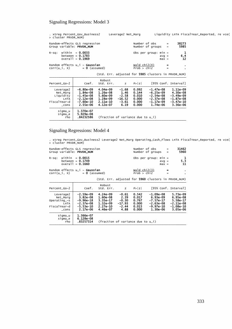
333
Signaling Regressions: Model 3
Signaling Regressions: Model 4
rho .84232586 (fraction of variance due to u_i) sigma_e 5.929e-08 sigma_u 1.370e-07 _cons 2.55e-06 4.12e-07 6.19 0.000 1.74e-06 3.36e-06FiscalYear~d -7.60e-10 2.11e-10 -3.61 0.000 -1.17e-09 -3.47e-10 LnTA -2.12e-08 1.28e-09 -16.52 0.000 -2.37e-08 -1.87e-08 Liquidity -1.45e-08 5.60e-09 -2.58 0.010 -2.54e-08 -3.49e-09 Net_Marg 1.84e-08 1.26e-08 1.46 0.144 -6.25e-09 4.30e-08 Leverage2 -6.80e-09 4.04e-09 -1.68 0.092 -1.47e-08 1.11e-09 Percent_Go~2 Coef. Std. Err. z P>|z| [95% Conf. Interval] Robust (Std. Err. adjusted for 5985 clusters in PRVDR_NUM)
corr(u_i, X) = 0 (assumed) Prob > chi2 = .Random effects u_i ~ Gaussian Wald chi2(4) = .
overall = 0.1969 max = 12 between = 0.1783 avg = 6.4R-sq: within = 0.0033 Obs per group: min = 1
Group variable: PRVDR_NUM Number of groups = 5985Random-effects GLS regression Number of obs = 38273
> cluster PRVDR_NUM). xtreg Percent_Gov_Business2 Leverage2 Net_Marg Liquidity LnTA FiscalYear_Reported, re vce(
rho .83257314 (fraction of variance due to u_i) sigma_e 6.128e-08 sigma_u 1.366e-07 _cons 2.17e-06 4.46e-07 4.88 0.000 1.30e-06 3.05e-06FiscalYear~d -5.53e-10 2.27e-10 -2.44 0.015 -9.97e-10 -1.08e-10 LnTA -2.37e-08 1.32e-09 -17.93 0.000 -2.63e-08 -2.11e-08Operating_~s -9.96e-18 3.35e-17 -0.30 0.767 -7.57e-17 5.58e-17 Net_Marg 3.82e-08 1.60e-08 2.39 0.017 6.93e-09 6.95e-08 Leverage2 -2.59e-09 4.24e-09 -0.61 0.542 -1.09e-08 5.73e-09 Percent_Go~2 Coef. Std. Err. z P>|z| [95% Conf. Interval] Robust (Std. Err. adjusted for 5960 clusters in PRVDR_NUM)
corr(u_i, X) = 0 (assumed) Prob > chi2 = .Random effects u_i ~ Gaussian Wald chi2(3) = .
overall = 0.1660 max = 11 between = 0.1749 avg = 5.3R-sq: within = 0.0015 Obs per group: min = 1
Group variable: PRVDR_NUM Number of groups = 5960Random-effects GLS regression Number of obs = 31462
> cluster PRVDR_NUM). xtreg Percent_Gov_Business2 Leverage2 Net_Marg Operating_Cash_Flows LnTA FiscalYear_Reported, re vce(
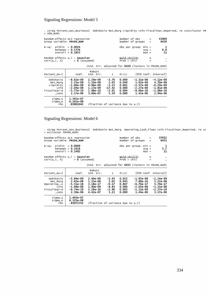
334
Signaling Regressions: Model 5
Signaling Regressions: Model 6
rho .83861042 (fraction of variance due to u_i) sigma_e 6.101e-08 sigma_u 1.391e-07 _cons 2.17e-06 3.89e-07 5.59 0.000 1.41e-06 2.94e-06FiscalYear~d -5.77e-10 1.98e-10 -2.91 0.004 -9.66e-10 -1.88e-10 LnTA -2.04e-08 1.17e-09 -17.42 0.000 -2.27e-08 -1.81e-08 Liquidity -1.60e-08 4.96e-09 -3.23 0.001 -2.57e-08 -6.29e-09 Net_Marg 2.25e-08 1.10e-08 2.05 0.040 1.02e-09 4.39e-08 DebtRatio -8.62e-09 2.29e-09 -3.76 0.000 -1.31e-08 -4.12e-09 Percent_Go~2 Coef. Std. Err. z P>|z| [95% Conf. Interval] Robust (Std. Err. adjusted for 6420 clusters in PRVDR_NUM)
corr(u_i, X) = 0 (assumed) Prob > chi2 = .Random effects u_i ~ Gaussian Wald chi2(4) = .
overall = 0.1853 max = 11 between = 0.1734 avg = 6.8R-sq: within = 0.0024 Obs per group: min = 1
Group variable: PRVDR_NUM Number of groups = 6420Random-effects GLS regression Number of obs = 43909
> VDR_NUM). xtreg Percent_Gov_Business2 DebtRatio Net_Marg Liquidity LnTA FiscalYear_Reported, re vce(cluster PR
rho .83071742 (fraction of variance due to u_i) sigma_e 6.335e-08 sigma_u 1.403e-07 _cons 2.30e-06 4.42e-07 5.21 0.000 1.44e-06 3.17e-06FiscalYear~d -6.74e-10 2.28e-10 -2.96 0.003 -1.12e-09 -2.27e-10 LnTA -1.68e-08 1.90e-09 -8.83 0.000 -2.05e-08 -1.31e-08Operating_~s -5.31e-18 3.18e-17 -0.17 0.867 -6.76e-17 5.70e-17 Net_Marg 2.65e-08 1.31e-08 2.02 0.043 7.88e-10 5.22e-08 DebtRatio -5.84e-09 2.40e-09 -2.43 0.015 -1.05e-08 -1.14e-09 Percent_Go~2 Coef. Std. Err. z P>|z| [95% Conf. Interval] Robust (Std. Err. adjusted for 6455 clusters in PRVDR_NUM)
corr(u_i, X) = 0 (assumed) Prob > chi2 = .Random effects u_i ~ Gaussian Wald chi2(3) = .
overall = 0.1492 max = 11 between = 0.1616 avg = 5.7R-sq: within = 0.0009 Obs per group: min = 1
Group variable: PRVDR_NUM Number of groups = 6455Random-effects GLS regression Number of obs = 37052
> e(cluster PRVDR_NUM). xtreg Percent_Gov_Business2 DebtRatio Net_Marg Operating_Cash_Flows LnTA FiscalYear_Reported, re vc
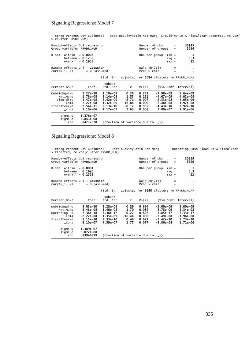
335
Signaling Regressions: Model 7
Signaling Regressions: Model 8
rho .84712878 (fraction of variance due to u_i) sigma_e 5.843e-08 sigma_u 1.376e-07 _cons 1.10e-06 4.17e-07 2.63 0.008 2.80e-07 1.91e-06FiscalYear~d -2.54e-11 2.13e-10 -0.12 0.905 -4.43e-10 3.92e-10 LnTA -2.22e-08 1.32e-09 -16.84 0.000 -2.48e-08 -1.97e-08 Liquidity -1.47e-08 5.42e-09 -2.71 0.007 -2.53e-08 -4.05e-09 Net_Marg 1.78e-08 1.14e-08 1.55 0.121 -4.67e-09 4.02e-08DebtToEqui~o 3.27e-10 1.18e-09 0.28 0.781 -1.98e-09 2.64e-09 Percent_Go~2 Coef. Std. Err. z P>|z| [95% Conf. Interval] Robust (Std. Err. adjusted for 5694 clusters in PRVDR_NUM)
corr(u_i, X) = 0 (assumed) Prob > chi2 = .Random effects u_i ~ Gaussian Wald chi2(4) = .
overall = 0.1933 max = 11 between = 0.1738 avg = 6.3R-sq: within = 0.0006 Obs per group: min = 1
Group variable: PRVDR_NUM Number of groups = 5694Random-effects GLS regression Number of obs = 36145
> cluster PRVDR_NUM). xtreg Percent_Gov_Business2 DebtToEquityRatio Net_Marg Liquidity LnTA FiscalYear_Reported, re vce(
rho .83946899 (fraction of variance due to u_i) sigma_e 6.072e-08 sigma_u 1.389e-07 _cons 8.10e-07 4.59e-07 1.77 0.077 -8.86e-08 1.71e-06FiscalYear~d 1.15e-10 2.33e-10 0.49 0.621 -3.42e-10 5.73e-10 LnTA -2.22e-08 1.35e-09 -16.44 0.000 -2.49e-08 -1.96e-08Operating_~s 7.38e-18 3.36e-17 0.22 0.826 -5.85e-17 7.33e-17 Net_Marg 2.48e-08 1.46e-08 1.70 0.089 -3.78e-09 5.34e-08DebtToEqui~o 5.03e-10 1.28e-09 0.39 0.694 -2.00e-09 3.00e-09 Percent_Go~2 Coef. Std. Err. z P>|z| [95% Conf. Interval] Robust (Std. Err. adjusted for 5690 clusters in PRVDR_NUM)
corr(u_i, X) = 0 (assumed) Prob > chi2 = .Random effects u_i ~ Gaussian Wald chi2(3) = .
overall = 0.1558 max = 11 between = 0.1620 avg = 5.3R-sq: within = 0.0001 Obs per group: min = 1
Group variable: PRVDR_NUM Number of groups = 5690Random-effects GLS regression Number of obs = 30229
> Reported, re vce(cluster PRVDR_NUM). xtreg Percent_Gov_Business2 DebtToEquityRatio Net_Marg Operating_Cash_Flows LnTA FiscalYear_
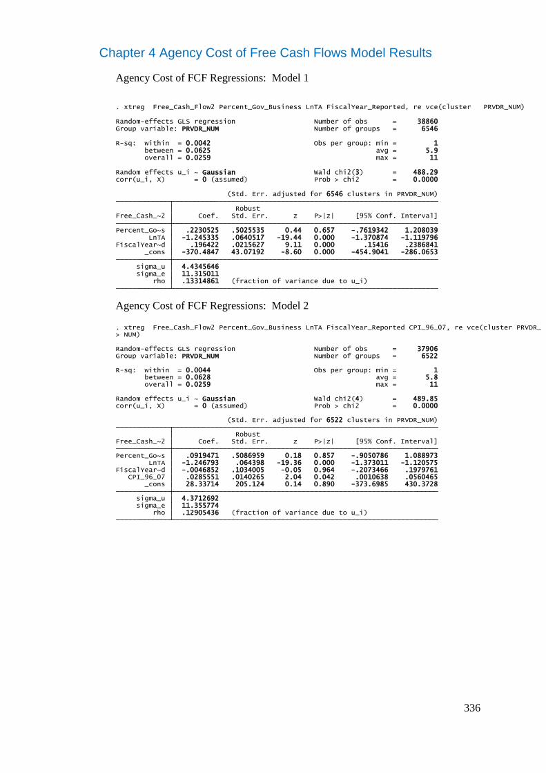
336
Chapter 4 Agency Cost of Free Cash Flows Model Results
Agency Cost of FCF Regressions: Model 1
Agency Cost of FCF Regressions: Model 2
rho .13314861 (fraction of variance due to u_i) sigma_e 11.315011 sigma_u 4.4345646 _cons -370.4847 43.07192 -8.60 0.000 -454.9041 -286.0653FiscalYear~d .196422 .0215627 9.11 0.000 .15416 .2386841 LnTA -1.245335 .0640517 -19.44 0.000 -1.370874 -1.119796Percent_Go~s .2230525 .5025535 0.44 0.657 -.7619342 1.208039 Free_Cash_~2 Coef. Std. Err. z P>|z| [95% Conf. Interval] Robust (Std. Err. adjusted for 6546 clusters in PRVDR_NUM)
corr(u_i, X) = 0 (assumed) Prob > chi2 = 0.0000Random effects u_i ~ Gaussian Wald chi2(3) = 488.29
overall = 0.0259 max = 11 between = 0.0625 avg = 5.9R-sq: within = 0.0042 Obs per group: min = 1
Group variable: PRVDR_NUM Number of groups = 6546Random-effects GLS regression Number of obs = 38860
. xtreg Free_Cash_Flow2 Percent_Gov_Business LnTA FiscalYear_Reported, re vce(cluster PRVDR_NUM)
rho .12905436 (fraction of variance due to u_i) sigma_e 11.355774 sigma_u 4.3712692 _cons 28.33714 205.124 0.14 0.890 -373.6985 430.3728 CPI_96_07 .0285551 .0140265 2.04 0.042 .0010638 .0560465FiscalYear~d -.0046852 .1034005 -0.05 0.964 -.2073466 .1979761 LnTA -1.246793 .064398 -19.36 0.000 -1.373011 -1.120575Percent_Go~s .0919471 .5086959 0.18 0.857 -.9050786 1.088973 Free_Cash_~2 Coef. Std. Err. z P>|z| [95% Conf. Interval] Robust (Std. Err. adjusted for 6522 clusters in PRVDR_NUM)
corr(u_i, X) = 0 (assumed) Prob > chi2 = 0.0000Random effects u_i ~ Gaussian Wald chi2(4) = 489.85
overall = 0.0259 max = 11 between = 0.0628 avg = 5.8R-sq: within = 0.0044 Obs per group: min = 1
Group variable: PRVDR_NUM Number of groups = 6522Random-effects GLS regression Number of obs = 37906
> NUM). xtreg Free_Cash_Flow2 Percent_Gov_Business LnTA FiscalYear_Reported CPI_96_07, re vce(cluster PRVDR_
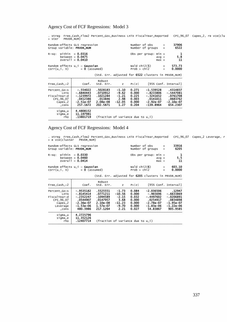
337
Agency Cost of FCF Regressions: Model 3
Agency Cost of FCF Regressions: Model 4
rho .13801719 (fraction of variance due to u_i) sigma_e 11.197981 sigma_u 4.4808152 _cons 257.1672 202.5871 1.27 0.204 -139.8964 654.2307 Capex_2 -2.51e-07 2.08e-08 -12.05 0.000 -2.92e-07 -2.10e-07 CPI_96_07 .0412386 .013846 2.98 0.003 .0141011 .0683762FiscalYear~d -.1239972 .1021284 -1.21 0.225 -.3241652 .0761708 LnTA -.6840443 .0710912 -9.62 0.000 -.8233806 -.5447081Percent_Go~s -.554022 .5028183 -1.10 0.271 -1.539528 .4314837 Free_Cash_~2 Coef. Std. Err. z P>|z| [95% Conf. Interval] Robust (Std. Err. adjusted for 6522 clusters in PRVDR_NUM)
corr(u_i, X) = 0 (assumed) Prob > chi2 = 0.0000Random effects u_i ~ Gaussian Wald chi2(5) = 573.73
overall = 0.0410 max = 11 between = 0.0475 avg = 5.8R-sq: within = 0.0316 Obs per group: min = 1
Group variable: PRVDR_NUM Number of groups = 6522Random-effects GLS regression Number of obs = 37906
> ster PRVDR_NUM). xtreg Free_Cash_Flow2 Percent_Gov_Business LnTA FiscalYear_Reported CPI_96_07 Capex_2, re vce(clu
rho .12407714 (fraction of variance due to u_i) sigma_e 11.352126 sigma_u 4.2725796 _cons 480.3986 217.1264 2.21 0.027 54.83867 905.9585 Leverage -1.53e-06 1.57e-07 -9.70 0.000 -1.83e-06 -1.22e-06 Capex_2 -2.36e-07 2.10e-08 -11.23 0.000 -2.78e-07 -1.95e-07 CPI_96_07 .0544907 .0147957 3.68 0.000 .0254917 .0834898FiscalYear~d -.2352247 .1094589 -2.15 0.032 -.4497602 -.0206891 LnTA -.8145414 .0771211 -10.56 0.000 -.965696 -.6633869Percent_Go~s -.9535182 .5525551 -1.73 0.084 -2.036506 .12947 Free_Cash_~2 Coef. Std. Err. z P>|z| [95% Conf. Interval] Robust (Std. Err. adjusted for 6205 clusters in PRVDR_NUM)
corr(u_i, X) = 0 (assumed) Prob > chi2 = 0.0000Random effects u_i ~ Gaussian Wald chi2(6) = 603.10
overall = 0.0414 max = 11 between = 0.0460 avg = 5.5R-sq: within = 0.0330 Obs per group: min = 1
Group variable: PRVDR_NUM Number of groups = 6205Random-effects GLS regression Number of obs = 33916
> e vce(cluster PRVDR_NUM). xtreg Free_Cash_Flow2 Percent_Gov_Business LnTA FiscalYear_Reported CPI_96_07 Capex_2 Leverage, r
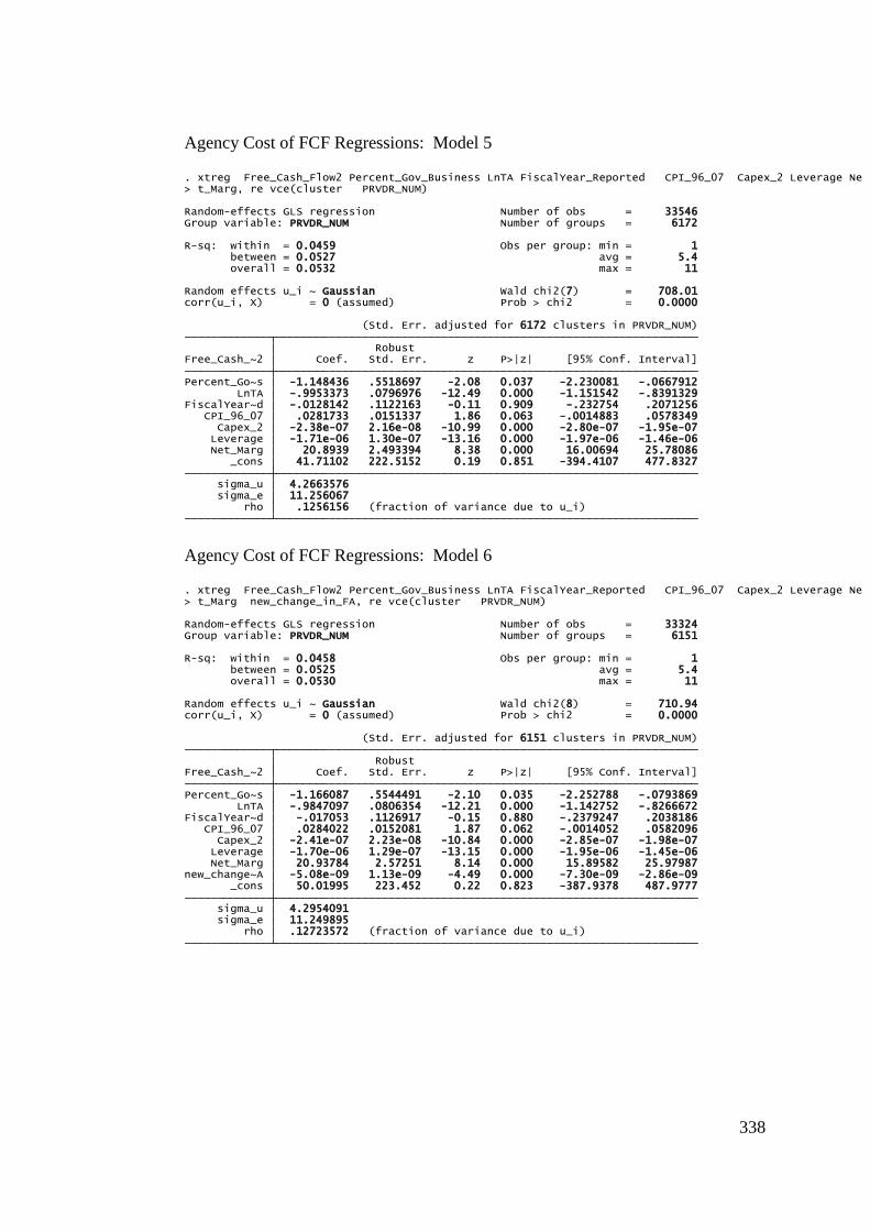
338
Agency Cost of FCF Regressions: Model 5
Agency Cost of FCF Regressions: Model 6
rho .1256156 (fraction of variance due to u_i) sigma_e 11.256067 sigma_u 4.2663576 _cons 41.71102 222.5152 0.19 0.851 -394.4107 477.8327 Net_Marg 20.8939 2.493394 8.38 0.000 16.00694 25.78086 Leverage -1.71e-06 1.30e-07 -13.16 0.000 -1.97e-06 -1.46e-06 Capex_2 -2.38e-07 2.16e-08 -10.99 0.000 -2.80e-07 -1.95e-07 CPI_96_07 .0281733 .0151337 1.86 0.063 -.0014883 .0578349FiscalYear~d -.0128142 .1122163 -0.11 0.909 -.232754 .2071256 LnTA -.9953373 .0796976 -12.49 0.000 -1.151542 -.8391329Percent_Go~s -1.148436 .5518697 -2.08 0.037 -2.230081 -.0667912 Free_Cash_~2 Coef. Std. Err. z P>|z| [95% Conf. Interval] Robust (Std. Err. adjusted for 6172 clusters in PRVDR_NUM)
corr(u_i, X) = 0 (assumed) Prob > chi2 = 0.0000Random effects u_i ~ Gaussian Wald chi2(7) = 708.01
overall = 0.0532 max = 11 between = 0.0527 avg = 5.4R-sq: within = 0.0459 Obs per group: min = 1
Group variable: PRVDR_NUM Number of groups = 6172Random-effects GLS regression Number of obs = 33546
> t_Marg, re vce(cluster PRVDR_NUM). xtreg Free_Cash_Flow2 Percent_Gov_Business LnTA FiscalYear_Reported CPI_96_07 Capex_2 Leverage Ne
rho .12723572 (fraction of variance due to u_i) sigma_e 11.249895 sigma_u 4.2954091 _cons 50.01995 223.452 0.22 0.823 -387.9378 487.9777new_change~A -5.08e-09 1.13e-09 -4.49 0.000 -7.30e-09 -2.86e-09 Net_Marg 20.93784 2.57251 8.14 0.000 15.89582 25.97987 Leverage -1.70e-06 1.29e-07 -13.15 0.000 -1.95e-06 -1.45e-06 Capex_2 -2.41e-07 2.23e-08 -10.84 0.000 -2.85e-07 -1.98e-07 CPI_96_07 .0284022 .0152081 1.87 0.062 -.0014052 .0582096FiscalYear~d -.017053 .1126917 -0.15 0.880 -.2379247 .2038186 LnTA -.9847097 .0806354 -12.21 0.000 -1.142752 -.8266672Percent_Go~s -1.166087 .5544491 -2.10 0.035 -2.252788 -.0793869 Free_Cash_~2 Coef. Std. Err. z P>|z| [95% Conf. Interval] Robust (Std. Err. adjusted for 6151 clusters in PRVDR_NUM)
corr(u_i, X) = 0 (assumed) Prob > chi2 = 0.0000Random effects u_i ~ Gaussian Wald chi2(8) = 710.94
overall = 0.0530 max = 11 between = 0.0525 avg = 5.4R-sq: within = 0.0458 Obs per group: min = 1
Group variable: PRVDR_NUM Number of groups = 6151Random-effects GLS regression Number of obs = 33324
> t_Marg new_change_in_FA, re vce(cluster PRVDR_NUM). xtreg Free_Cash_Flow2 Percent_Gov_Business LnTA FiscalYear_Reported CPI_96_07 Capex_2 Leverage Ne
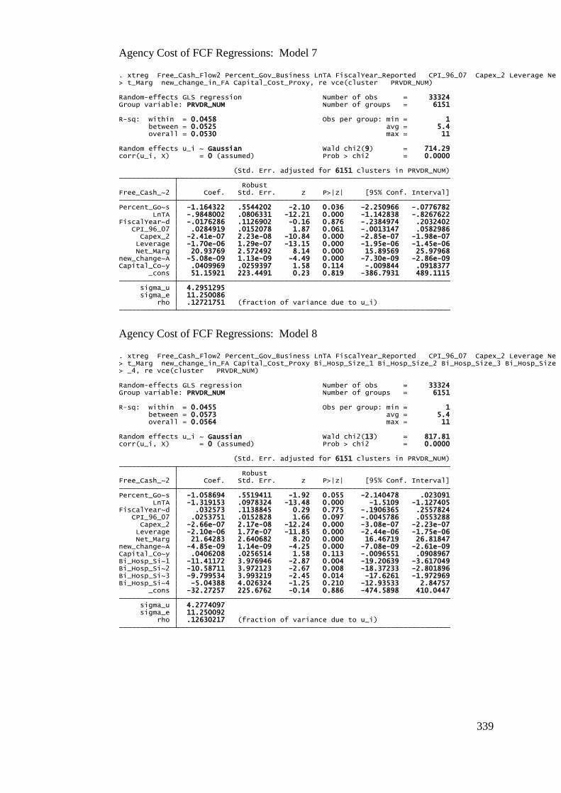
339
Agency Cost of FCF Regressions: Model 7
Agency Cost of FCF Regressions: Model 8
rho .12721751 (fraction of variance due to u_i) sigma_e 11.250086 sigma_u 4.2951295 _cons 51.15921 223.4491 0.23 0.819 -386.7931 489.1115Capital_Co~y .0409969 .0259397 1.58 0.114 -.009844 .0918377new_change~A -5.08e-09 1.13e-09 -4.49 0.000 -7.30e-09 -2.86e-09 Net_Marg 20.93769 2.572492 8.14 0.000 15.89569 25.97968 Leverage -1.70e-06 1.29e-07 -13.15 0.000 -1.95e-06 -1.45e-06 Capex_2 -2.41e-07 2.23e-08 -10.84 0.000 -2.85e-07 -1.98e-07 CPI_96_07 .0284919 .0152078 1.87 0.061 -.0013147 .0582986FiscalYear~d -.0176286 .1126902 -0.16 0.876 -.2384974 .2032402 LnTA -.9848002 .0806331 -12.21 0.000 -1.142838 -.8267622Percent_Go~s -1.164322 .5544202 -2.10 0.036 -2.250966 -.0776782 Free_Cash_~2 Coef. Std. Err. z P>|z| [95% Conf. Interval] Robust (Std. Err. adjusted for 6151 clusters in PRVDR_NUM)
corr(u_i, X) = 0 (assumed) Prob > chi2 = 0.0000Random effects u_i ~ Gaussian Wald chi2(9) = 714.29
overall = 0.0530 max = 11 between = 0.0525 avg = 5.4R-sq: within = 0.0458 Obs per group: min = 1
Group variable: PRVDR_NUM Number of groups = 6151Random-effects GLS regression Number of obs = 33324
> t_Marg new_change_in_FA Capital_Cost_Proxy, re vce(cluster PRVDR_NUM). xtreg Free_Cash_Flow2 Percent_Gov_Business LnTA FiscalYear_Reported CPI_96_07 Capex_2 Leverage Ne
rho .12630217 (fraction of variance due to u_i) sigma_e 11.250092 sigma_u 4.2774097 _cons -32.27257 225.6762 -0.14 0.886 -474.5898 410.0447Bi_Hosp_Si~4 -5.04388 4.026324 -1.25 0.210 -12.93533 2.84757Bi_Hosp_Si~3 -9.799534 3.993219 -2.45 0.014 -17.6261 -1.972969Bi_Hosp_Si~2 -10.58711 3.972123 -2.67 0.008 -18.37233 -2.801896Bi_Hosp_Si~1 -11.41172 3.976946 -2.87 0.004 -19.20639 -3.617049Capital_Co~y .0406208 .0256514 1.58 0.113 -.0096551 .0908967new_change~A -4.85e-09 1.14e-09 -4.25 0.000 -7.08e-09 -2.61e-09 Net_Marg 21.64283 2.640682 8.20 0.000 16.46719 26.81847 Leverage -2.10e-06 1.77e-07 -11.85 0.000 -2.44e-06 -1.75e-06 Capex_2 -2.66e-07 2.17e-08 -12.24 0.000 -3.08e-07 -2.23e-07 CPI_96_07 .0253751 .0152828 1.66 0.097 -.0045786 .0553288FiscalYear~d .032573 .1138845 0.29 0.775 -.1906365 .2557824 LnTA -1.319153 .0978324 -13.48 0.000 -1.5109 -1.127405Percent_Go~s -1.058694 .5519411 -1.92 0.055 -2.140478 .023091 Free_Cash_~2 Coef. Std. Err. z P>|z| [95% Conf. Interval] Robust (Std. Err. adjusted for 6151 clusters in PRVDR_NUM)
corr(u_i, X) = 0 (assumed) Prob > chi2 = 0.0000Random effects u_i ~ Gaussian Wald chi2(13) = 817.81
overall = 0.0564 max = 11 between = 0.0573 avg = 5.4R-sq: within = 0.0455 Obs per group: min = 1
Group variable: PRVDR_NUM Number of groups = 6151Random-effects GLS regression Number of obs = 33324
> _4, re vce(cluster PRVDR_NUM)> t_Marg new_change_in_FA Capital_Cost_Proxy Bi_Hosp_Size_1 Bi_Hosp_Size_2 Bi_Hosp_Size_3 Bi_Hosp_Size. xtreg Free_Cash_Flow2 Percent_Gov_Business LnTA FiscalYear_Reported CPI_96_07 Capex_2 Leverage Ne
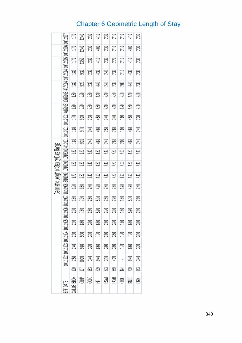
340
Chapter 6 Geometric Length of Stay
Geom
etric L
ength o
f Stay
by Dat
e Rang
eEF
F_DATE
10/1/1
99210/
1/1993
10/1/1
99410/
1/1995
10/1/1
99610/
1/1997
10/1/1
9983/1
/1999
10/1/1
99910/
1/2000
4/1/20
0110/
1/2001
10/1/2
0024/1
/2003
10/1/2
0034/1
/2004
10/1/2
00410/
1/2005
10/1/2
00610/
1/2007
GMLO
SBRO
N100
2.50
2.40
2.30
2.10
2.00
1.80
1.70
1.70
1.8
0
1.8
0
1.8
0
1.80
1.70
1.70
1.8
0
1.8
0
1.80
1.70
1.70
1.70
CBYP
10710.
20
9.80
9.30
8.60
7.80
7.30
9.50
9.50
9.3
0
9.2
0
9.2
0
9.70
9.20
9.20
9.2
0
9.2
0
9.30
13.50
12.
40
12.40
COLO
1833.4
0
3.2
0
3.1
0
3.0
0
2.8
0
2.6
0
2.4
0
2.4
0
2.40
2.40
2.40
2.4
0
2.3
0
2.3
0
2.30
2.30
2.3
0
2.3
0
2.3
0
2.3
0
HIP209
9.40
8.60
7.70
6.80
5.90
5.30
4.90
4.90
4.6
0
4.6
0
4.6
0
4.60
4.50
4.50
4.4
0
4.4
0
4.30
4.10
4.00
4.10
ESWL
3233.1
0
3.0
0
2.9
0
2.8
0
2.7
0
2.5
0
2.4
0
2.4
0
2.40
2.40
2.40
2.5
0
2.4
0
2.4
0
2.40
2.40
2.4
0
2.3
0
2.3
0
2.3
0
LAVH
3594.2
0
3.9
0
3.5
0
3.2
0
3.0
0
2.9
0
2.8
0
2.8
0
2.70
2.60
2.60
2.6
0
2.4
0
2.4
0
2.30
2.30
2.3
0
2.2
0
2.1
0
2.1
0
CHOL
494-
1.70
1.70
1.80
1.80
1.80
1.90
1.90
2.0
0
2.0
0
2.0
0
1.90
1.90
1.90
2.0
0
2.0
0
2.10
2.10
2.10
2.10
KNEE
2099.4
0
8.6
0
7.7
0
6.8
0
5.9
0
5.3
0
4.9
0
4.9
0
4.60
4.60
4.60
4.6
0
4.5
0
4.5
0
4.40
4.40
4.3
0
4.1
0
4.0
0
4.1
0
EGD
1833.4
0
3.2
0
3.1
0
3.0
0
2.8
0
2.6
0
2.4
0
2.4
0
2.40
2.40
2.40
2.4
0
2.3
0
2.3
0
2.30
2.30
2.3
0
2.3
0
2.3
0
2.3
0
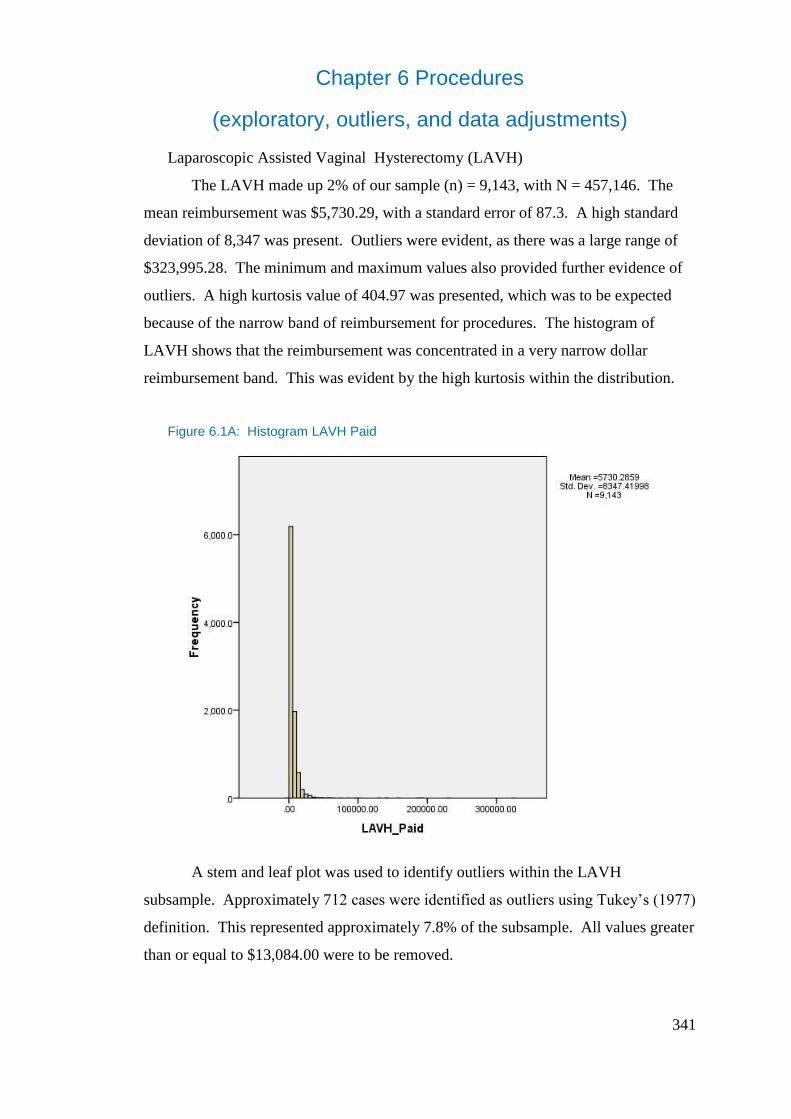
341
Chapter 6 Procedures
(exploratory, outliers, and data adjustments)
Laparoscopic Assisted Vaginal Hysterectomy (LAVH)
The LAVH made up 2% of our sample (n) = 9,143, with N = 457,146. The
mean reimbursement was $5,730.29, with a standard error of 87.3. A high standard
deviation of 8,347 was present. Outliers were evident, as there was a large range of
$323,995.28. The minimum and maximum values also provided further evidence of
outliers. A high kurtosis value of 404.97 was presented, which was to be expected
because of the narrow band of reimbursement for procedures. The histogram of
LAVH shows that the reimbursement was concentrated in a very narrow dollar
reimbursement band. This was evident by the high kurtosis within the distribution.
Figure 6.1A: Histogram LAVH Paid
A stem and leaf plot was used to identify outliers within the LAVH
subsample. Approximately 712 cases were identified as outliers using Tukey’s (1977)
definition. This represented approximately 7.8% of the subsample. All values greater
than or equal to $13,084.00 were to be removed.
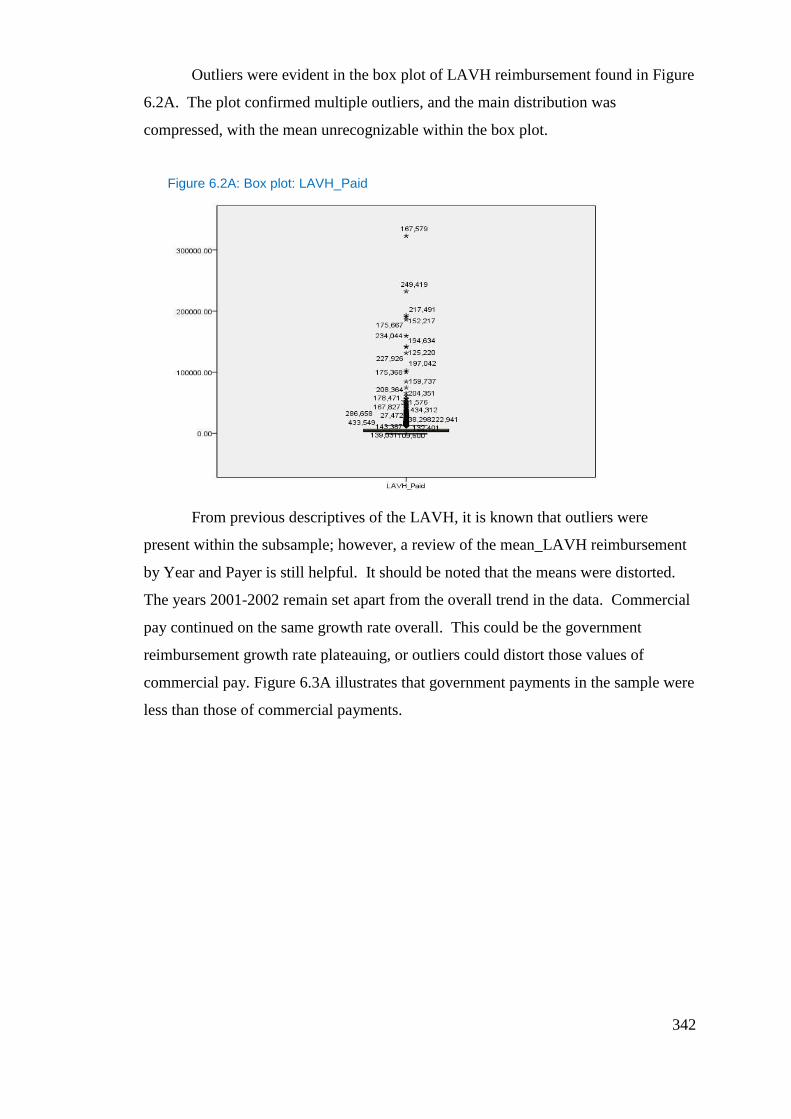
342
Outliers were evident in the box plot of LAVH reimbursement found in Figure
6.2A. The plot confirmed multiple outliers, and the main distribution was
compressed, with the mean unrecognizable within the box plot.
Figure 6.2A: Box plot: LAVH_Paid
From previous descriptives of the LAVH, it is known that outliers were
present within the subsample; however, a review of the mean_LAVH reimbursement
by Year and Payer is still helpful. It should be noted that the means were distorted.
The years 2001-2002 remain set apart from the overall trend in the data. Commercial
pay continued on the same growth rate overall. This could be the government
reimbursement growth rate plateauing, or outliers could distort those values of
commercial pay. Figure 6.3A illustrates that government payments in the sample were
less than those of commercial payments.
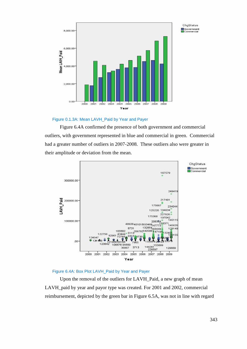
343
Figure 0.1.3A: Mean LAVH_Paid by Year and Payer
Figure 6.4A confirmed the presence of both government and commercial
outliers, with government represented in blue and commercial in green. Commercial
had a greater number of outliers in 2007-2008. These outliers also were greater in
their amplitude or deviation from the mean.
Figure 6.4A: Box Plot LAVH_Paid by Year and Payer
Upon the removal of the outliers for LAVH_Paid, a new graph of mean
LAVH_paid by year and payor type was created. For 2001 and 2002, commercial
reimbursement, depicted by the green bar in Figure 6.5A, was not in line with regard
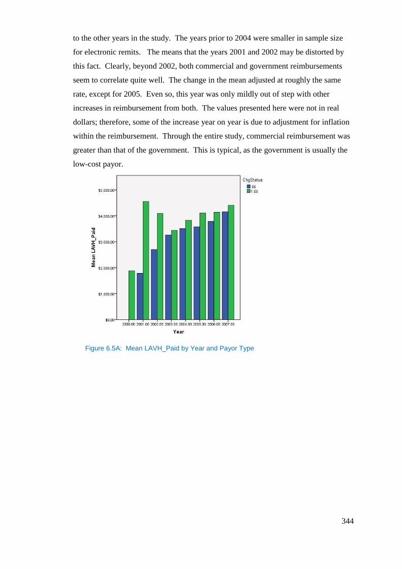
344
to the other years in the study. The years prior to 2004 were smaller in sample size
for electronic remits. The means that the years 2001 and 2002 may be distorted by
this fact. Clearly, beyond 2002, both commercial and government reimbursements
seem to correlate quite well. The change in the mean adjusted at roughly the same
rate, except for 2005. Even so, this year was only mildly out of step with other
increases in reimbursement from both. The values presented here were not in real
dollars; therefore, some of the increase year on year is due to adjustment for inflation
within the reimbursement. Through the entire study, commercial reimbursement was
greater than that of the government. This is typical, as the government is usually the
low-cost payor.
Figure 6.5A: Mean LAVH_Paid by Year and Payor Type
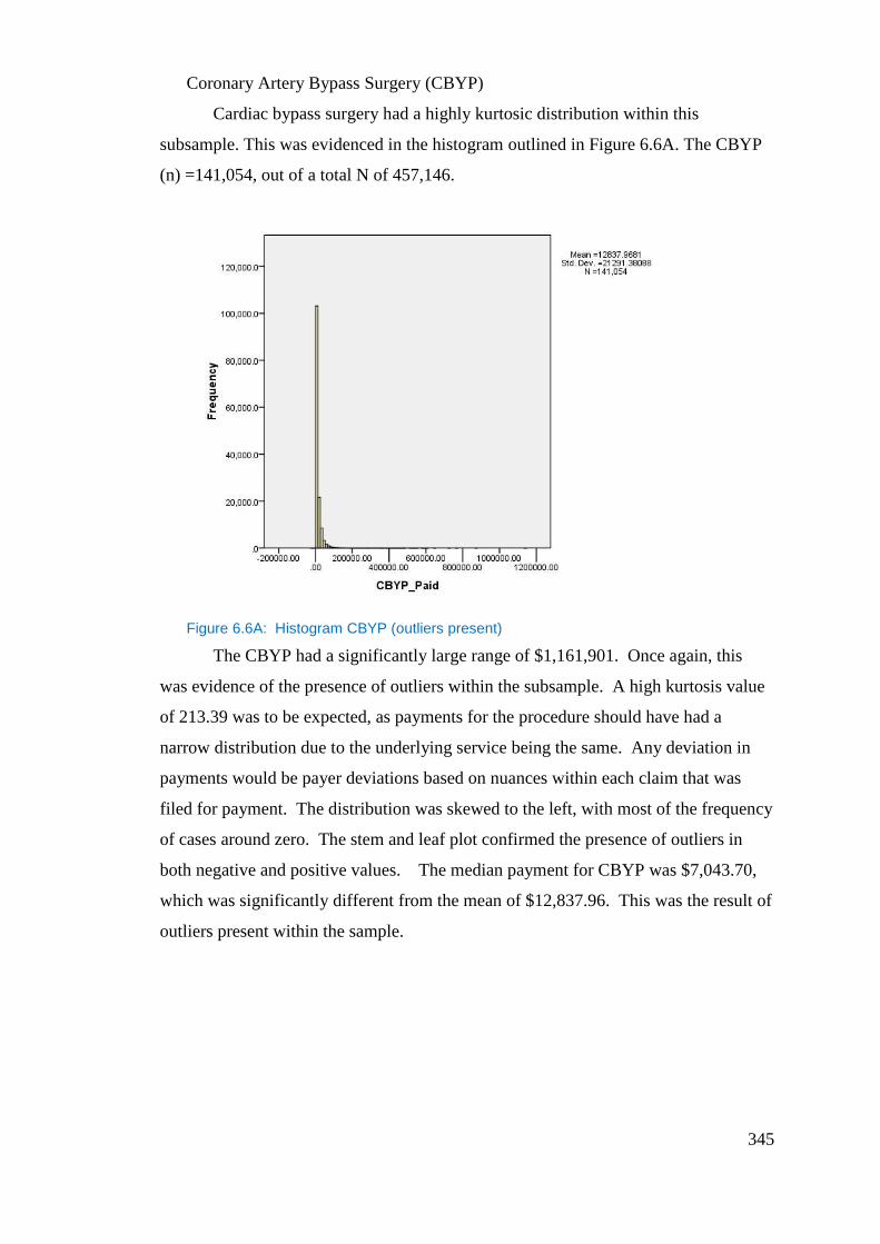
345
Coronary Artery Bypass Surgery (CBYP)
Cardiac bypass surgery had a highly kurtosic distribution within this
subsample. This was evidenced in the histogram outlined in Figure 6.6A. The CBYP
(n) =141,054, out of a total N of 457,146.
Figure 6.6A: Histogram CBYP (outliers present)
The CBYP had a significantly large range of $1,161,901. Once again, this
was evidence of the presence of outliers within the subsample. A high kurtosis value
of 213.39 was to be expected, as payments for the procedure should have had a
narrow distribution due to the underlying service being the same. Any deviation in
payments would be payer deviations based on nuances within each claim that was
filed for payment. The distribution was skewed to the left, with most of the frequency
of cases around zero. The stem and leaf plot confirmed the presence of outliers in
both negative and positive values. The median payment for CBYP was $7,043.70,
which was significantly different from the mean of $12,837.96. This was the result of
outliers present within the sample.
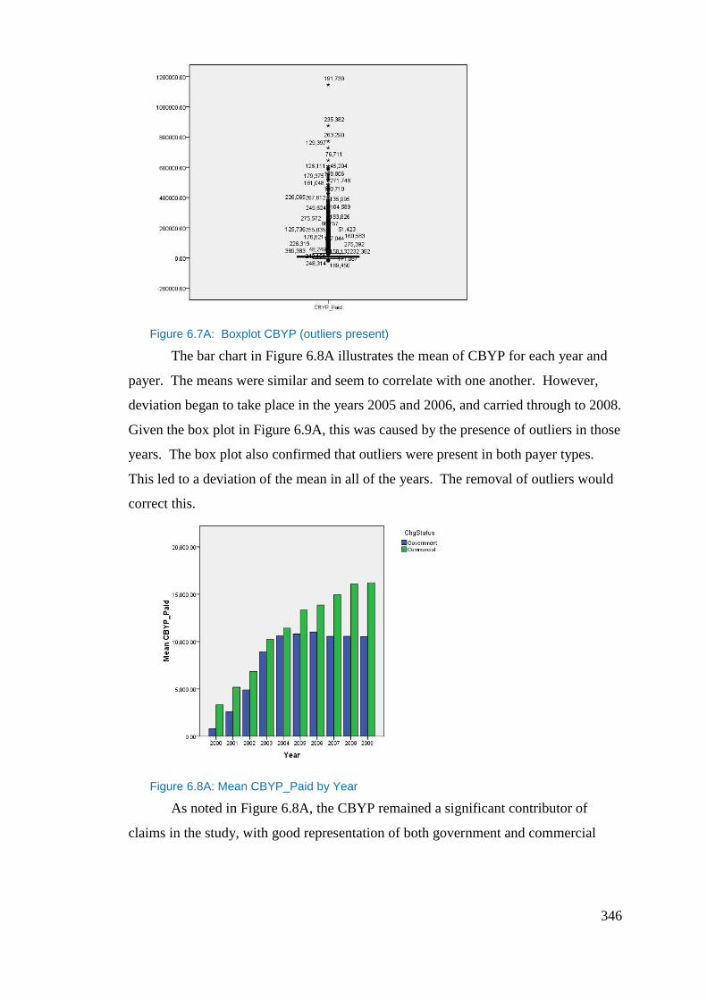
346
Figure 6.7A: Boxplot CBYP (outliers present)
The bar chart in Figure 6.8A illustrates the mean of CBYP for each year and
payer. The means were similar and seem to correlate with one another. However,
deviation began to take place in the years 2005 and 2006, and carried through to 2008.
Given the box plot in Figure 6.9A, this was caused by the presence of outliers in those
years. The box plot also confirmed that outliers were present in both payer types.
This led to a deviation of the mean in all of the years. The removal of outliers would
correct this.
Figure 6.8A: Mean CBYP_Paid by Year
As noted in Figure 6.8A, the CBYP remained a significant contributor of
claims in the study, with good representation of both government and commercial
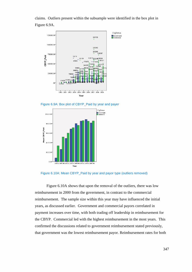
347
claims. Outliers present within the subsample were identified in the box plot in
Figure 6.9A.
Figure 6.9A: Box plot of CBYP_Paid by year and payer
Figure 6.10A: Mean CBYP_Paid by year and payor type (outliers removed)
Figure 6.10A shows that upon the removal of the outliers, there was low
reimbursement in 2000 from the government, in contrast to the commercial
reimbursement. The sample size within this year may have influenced the initial
years, as discussed earlier. Government and commercial payors correlated in
payment increases over time, with both trading off leadership in reimbursement for
the CBYP. Commercial led with the highest reimbursement in the most years. This
confirmed the discussions related to government reimbursement stated previously,
that government was the lowest reimbursement payor. Reimbursement rates for both
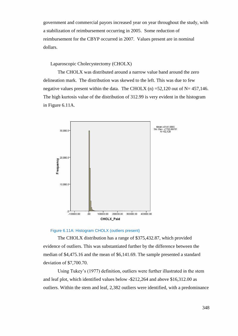
348
government and commercial payors increased year on year throughout the study, with
a stabilization of reimbursement occurring in 2005. Some reduction of
reimbursement for the CBYP occurred in 2007. Values present are in nominal
dollars.
Laparoscopic Cholecystectomy (CHOLX)
The CHOLX was distributed around a narrow value band around the zero
delineation mark. The distribution was skewed to the left. This was due to few
negative values present within the data. The CHOLX (n) =52,120 out of N= 457,146.
The high kurtosis value of the distribution of 312.99 is very evident in the histogram
in Figure 6.11A.
Figure 6.11A: Histogram CHOLX (outliers present)
The CHOLX distribution has a range of $375,432.87, which provided
evidence of outliers. This was substantiated further by the difference between the
median of $4,475.16 and the mean of $6,141.69. The sample presented a standard
deviation of $7,700.70.
Using Tukey’s (1977) definition, outliers were further illustrated in the stem
and leaf plot, which identified values below -$212,264 and above $16,312.00 as
outliers. Within the stem and leaf, 2,382 outliers were identified, with a predominance
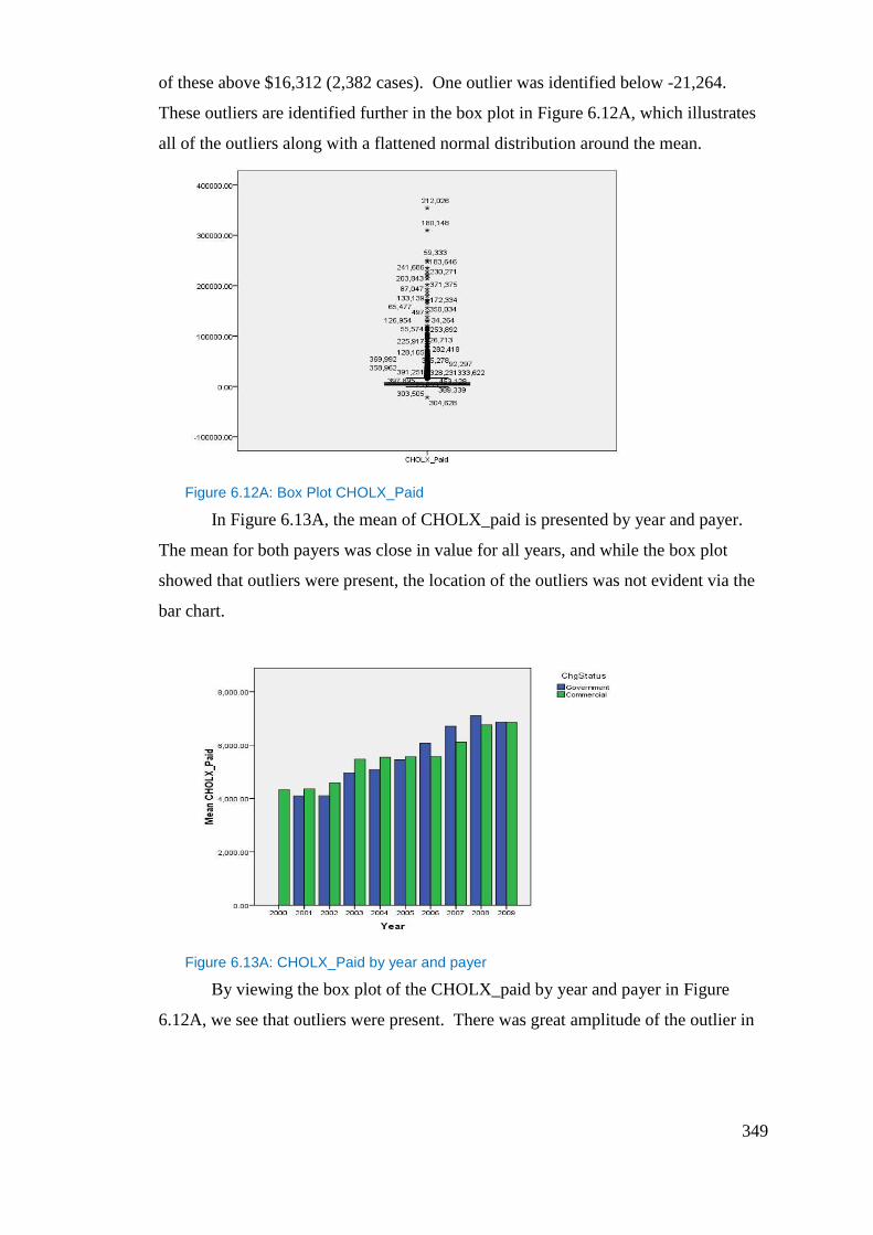
349
of these above $16,312 (2,382 cases). One outlier was identified below -21,264.
These outliers are identified further in the box plot in Figure 6.12A, which illustrates
all of the outliers along with a flattened normal distribution around the mean.
Figure 6.12A: Box Plot CHOLX_Paid
In Figure 6.13A, the mean of CHOLX_paid is presented by year and payer.
The mean for both payers was close in value for all years, and while the box plot
showed that outliers were present, the location of the outliers was not evident via the
bar chart.
Figure 6.13A: CHOLX_Paid by year and payer
By viewing the box plot of the CHOLX_paid by year and payer in Figure
6.12A, we see that outliers were present. There was great amplitude of the outlier in
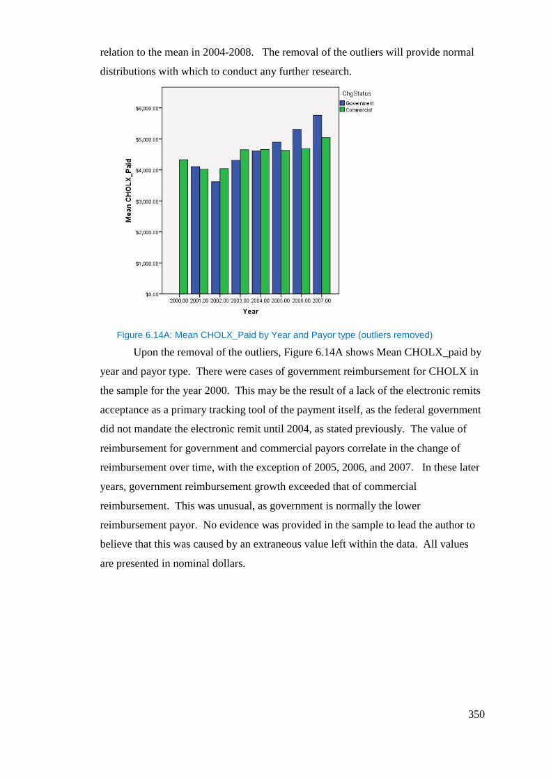
350
relation to the mean in 2004-2008. The removal of the outliers will provide normal
distributions with which to conduct any further research.
Figure 6.14A: Mean CHOLX_Paid by Year and Payor type (outliers removed)
Upon the removal of the outliers, Figure 6.14A shows Mean CHOLX_paid by
year and payor type. There were cases of government reimbursement for CHOLX in
the sample for the year 2000. This may be the result of a lack of the electronic remits
acceptance as a primary tracking tool of the payment itself, as the federal government
did not mandate the electronic remit until 2004, as stated previously. The value of
reimbursement for government and commercial payors correlate in the change of
reimbursement over time, with the exception of 2005, 2006, and 2007. In these later
years, government reimbursement growth exceeded that of commercial
reimbursement. This was unusual, as government is normally the lower
reimbursement payor. No evidence was provided in the sample to lead the author to
believe that this was caused by an extraneous value left within the data. All values
are presented in nominal dollars.
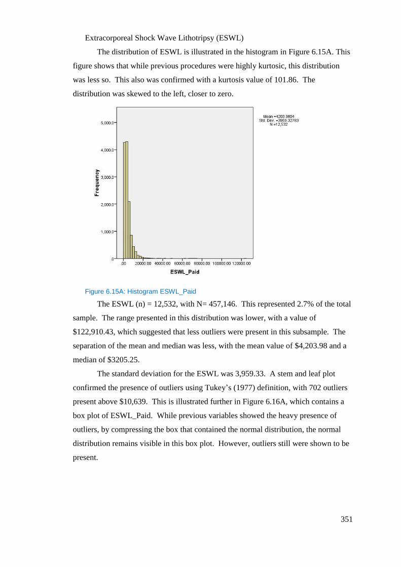
351
Extracorporeal Shock Wave Lithotripsy (ESWL)
The distribution of ESWL is illustrated in the histogram in Figure 6.15A. This
figure shows that while previous procedures were highly kurtosic, this distribution
was less so. This also was confirmed with a kurtosis value of 101.86. The
distribution was skewed to the left, closer to zero.
Figure 6.15A: Histogram ESWL_Paid
The ESWL (n) = 12,532, with N= 457,146. This represented 2.7% of the total
sample. The range presented in this distribution was lower, with a value of
$122,910.43, which suggested that less outliers were present in this subsample. The
separation of the mean and median was less, with the mean value of $4,203.98 and a
median of $3205.25.
The standard deviation for the ESWL was 3,959.33. A stem and leaf plot
confirmed the presence of outliers using Tukey’s (1977) definition, with 702 outliers
present above $10,639. This is illustrated further in Figure 6.16A, which contains a
box plot of ESWL_Paid. While previous variables showed the heavy presence of
outliers, by compressing the box that contained the normal distribution, the normal
distribution remains visible in this box plot. However, outliers still were shown to be
present.
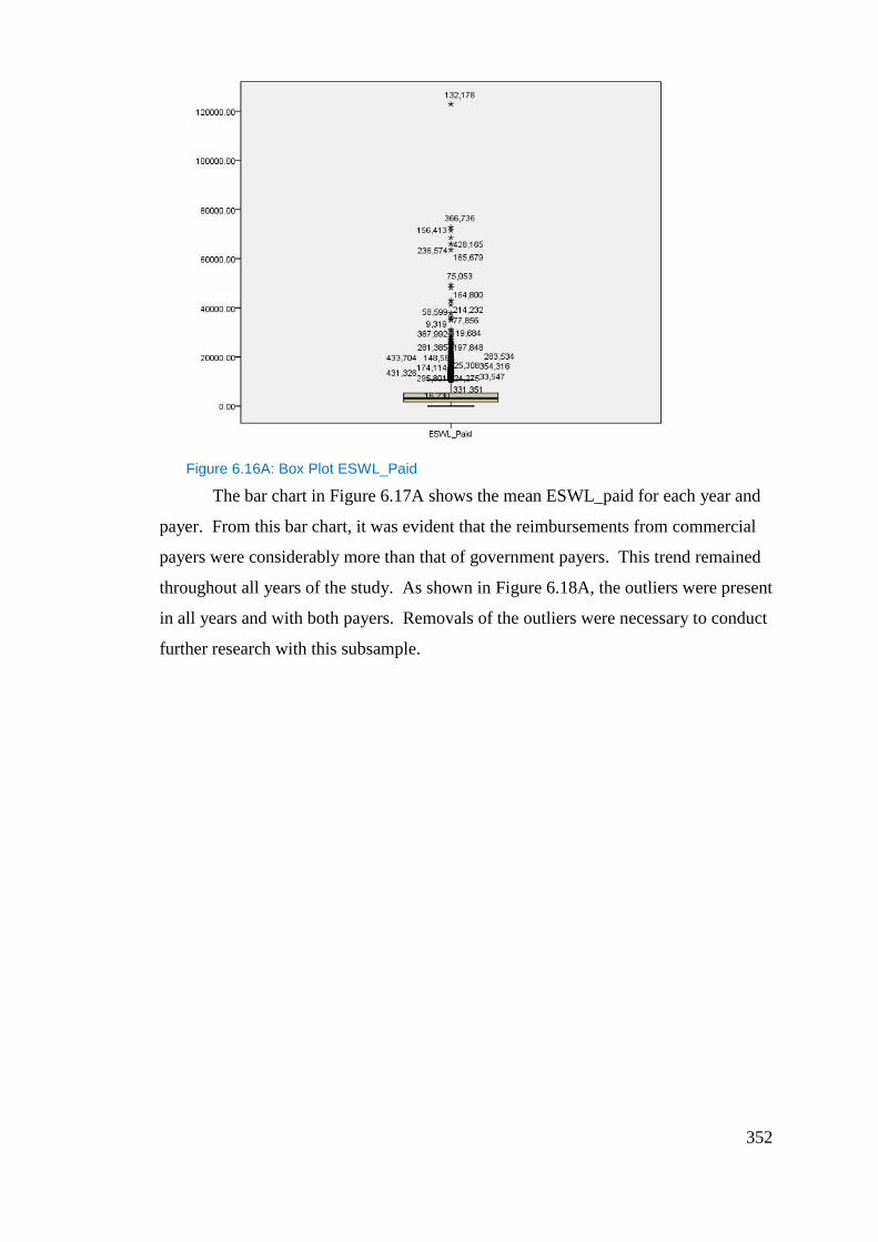
352
Figure 6.16A: Box Plot ESWL_Paid
The bar chart in Figure 6.17A shows the mean ESWL_paid for each year and
payer. From this bar chart, it was evident that the reimbursements from commercial
payers were considerably more than that of government payers. This trend remained
throughout all years of the study. As shown in Figure 6.18A, the outliers were present
in all years and with both payers. Removals of the outliers were necessary to conduct
further research with this subsample.
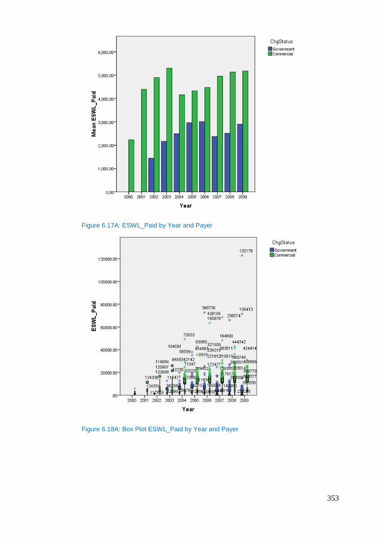
353
Figure 6.17A: ESWL_Paid by Year and Payer
Figure 6.18A: Box Plot ESWL_Paid by Year and Payer
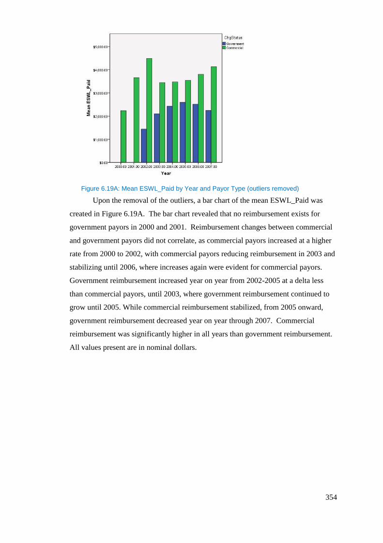
354
Figure 6.19A: Mean ESWL_Paid by Year and Payor Type (outliers removed)
Upon the removal of the outliers, a bar chart of the mean ESWL_Paid was
created in Figure 6.19A. The bar chart revealed that no reimbursement exists for
government payors in 2000 and 2001. Reimbursement changes between commercial
and government payors did not correlate, as commercial payors increased at a higher
rate from 2000 to 2002, with commercial payors reducing reimbursement in 2003 and
stabilizing until 2006, where increases again were evident for commercial payors.
Government reimbursement increased year on year from 2002-2005 at a delta less
than commercial payors, until 2003, where government reimbursement continued to
grow until 2005. While commercial reimbursement stabilized, from 2005 onward,
government reimbursement decreased year on year through 2007. Commercial
reimbursement was significantly higher in all years than government reimbursement.
All values present are in nominal dollars.
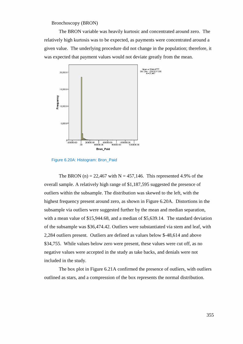
355
Bronchoscopy (BRON)
The BRON variable was heavily kurtosic and concentrated around zero. The
relatively high kurtosis was to be expected, as payments were concentrated around a
given value. The underlying procedure did not change in the population; therefore, it
was expected that payment values would not deviate greatly from the mean.
Figure 6.20A: Histogram: Bron_Paid
The BRON (n) = 22,467 with N = 457,146. This represented 4.9% of the
overall sample. A relatively high range of $1,187,595 suggested the presence of
outliers within the subsample. The distribution was skewed to the left, with the
highest frequency present around zero, as shown in Figure 6.20A. Distortions in the
subsample via outliers were suggested further by the mean and median separation,
with a mean value of $15,944.68, and a median of $5,639.14. The standard deviation
of the subsample was $36,474.42. Outliers were substantiated via stem and leaf, with
2,284 outliers present. Outliers are defined as values below $-48,614 and above
$34,755. While values below zero were present, these values were cut off, as no
negative values were accepted in the study as take backs, and denials were not
included in the study.
The box plot in Figure 6.21A confirmed the presence of outliers, with outliers
outlined as stars, and a compression of the box represents the normal distribution.
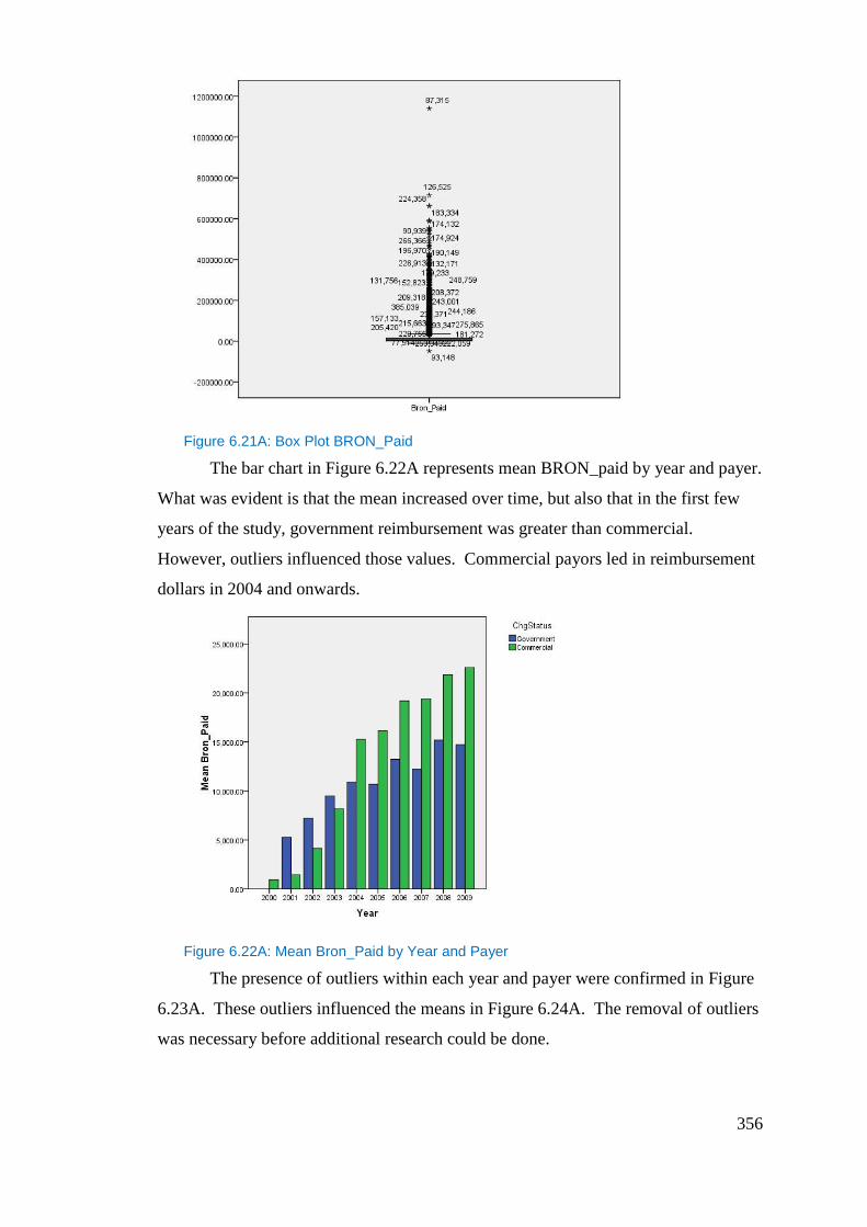
356
Figure 6.21A: Box Plot BRON_Paid
The bar chart in Figure 6.22A represents mean BRON_paid by year and payer.
What was evident is that the mean increased over time, but also that in the first few
years of the study, government reimbursement was greater than commercial.
However, outliers influenced those values. Commercial payors led in reimbursement
dollars in 2004 and onwards.
Figure 6.22A: Mean Bron_Paid by Year and Payer
The presence of outliers within each year and payer were confirmed in Figure
6.23A. These outliers influenced the means in Figure 6.24A. The removal of outliers
was necessary before additional research could be done.
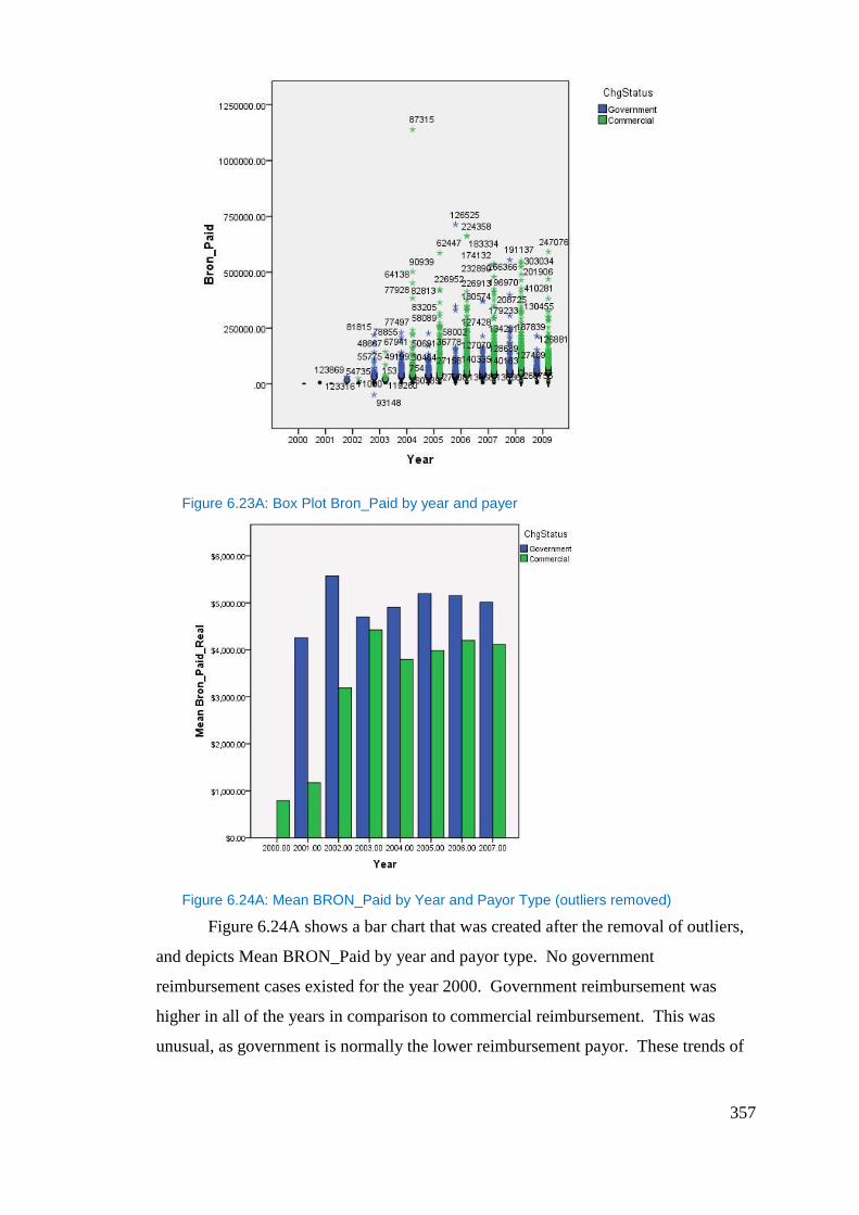
357
Figure 6.23A: Box Plot Bron_Paid by year and payer
Figure 6.24A: Mean BRON_Paid by Year and Payor Type (outliers removed)
Figure 6.24A shows a bar chart that was created after the removal of outliers,
and depicts Mean BRON_Paid by year and payor type. No government
reimbursement cases existed for the year 2000. Government reimbursement was
higher in all of the years in comparison to commercial reimbursement. This was
unusual, as government is normally the lower reimbursement payor. These trends of

358
higher payment existed throughout the entire time frame of the study. Changes in
reimbursement for government and commercial did not correlate at any time within
the time frame of the study. Both payors increased reimbursement for BRON
procedures year on year until 2004, when commercial payors reduced reimbursement.
A decrease in government reimbursement occurred two years later in 2006. The
differentiation in payment between government and commercial may have been
driven by the average age of the patients who receive bronchoscopies; however, this is
pure speculation by the author. All values presented are in nominal dollars.
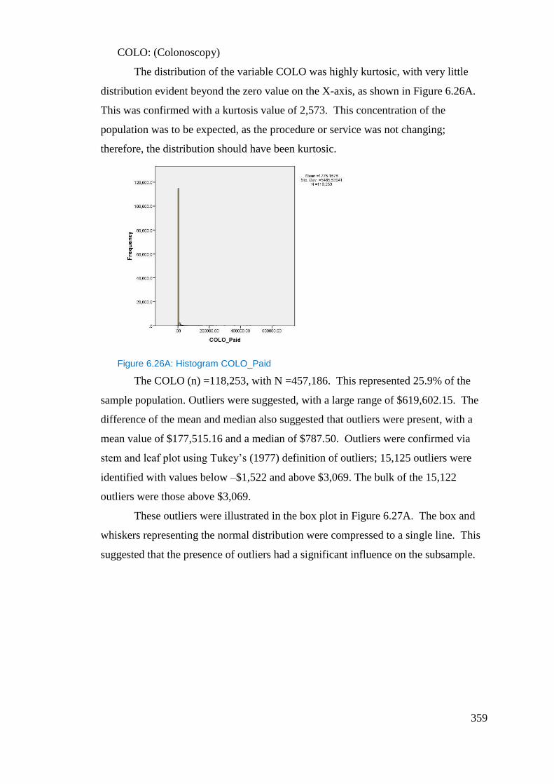
359
COLO: (Colonoscopy)
The distribution of the variable COLO was highly kurtosic, with very little
distribution evident beyond the zero value on the X-axis, as shown in Figure 6.26A.
This was confirmed with a kurtosis value of 2,573. This concentration of the
population was to be expected, as the procedure or service was not changing;
therefore, the distribution should have been kurtosic.
Figure 6.26A: Histogram COLO_Paid
The COLO (n) =118,253, with N =457,186. This represented 25.9% of the
sample population. Outliers were suggested, with a large range of $619,602.15. The
difference of the mean and median also suggested that outliers were present, with a
mean value of $177,515.16 and a median of $787.50. Outliers were confirmed via
stem and leaf plot using Tukey’s (1977) definition of outliers; 15,125 outliers were
identified with values below –$1,522 and above $3,069. The bulk of the 15,122
outliers were those above $3,069.
These outliers were illustrated in the box plot in Figure 6.27A. The box and
whiskers representing the normal distribution were compressed to a single line. This
suggested that the presence of outliers had a significant influence on the subsample.
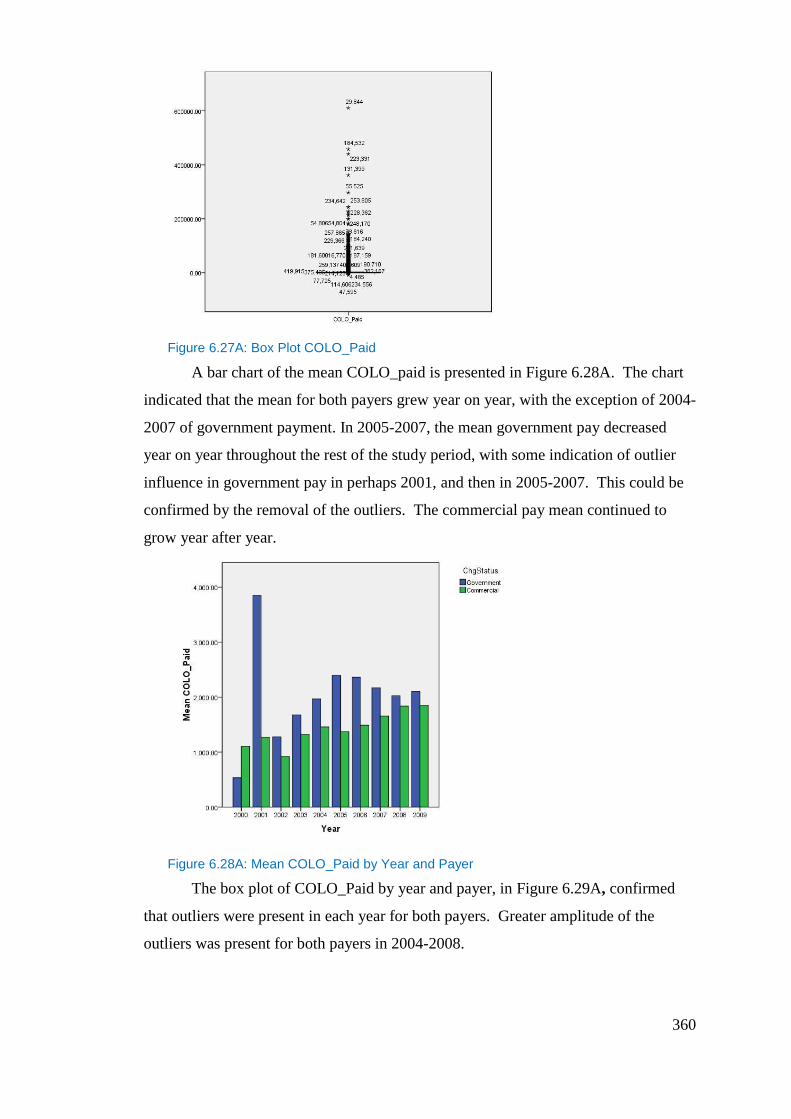
360
Figure 6.27A: Box Plot COLO_Paid
A bar chart of the mean COLO_paid is presented in Figure 6.28A. The chart
indicated that the mean for both payers grew year on year, with the exception of 2004-
2007 of government payment. In 2005-2007, the mean government pay decreased
year on year throughout the rest of the study period, with some indication of outlier
influence in government pay in perhaps 2001, and then in 2005-2007. This could be
confirmed by the removal of the outliers. The commercial pay mean continued to
grow year after year.
Figure 6.28A: Mean COLO_Paid by Year and Payer
The box plot of COLO_Paid by year and payer, in Figure 6.29A, confirmed
that outliers were present in each year for both payers. Greater amplitude of the
outliers was present for both payers in 2004-2008.
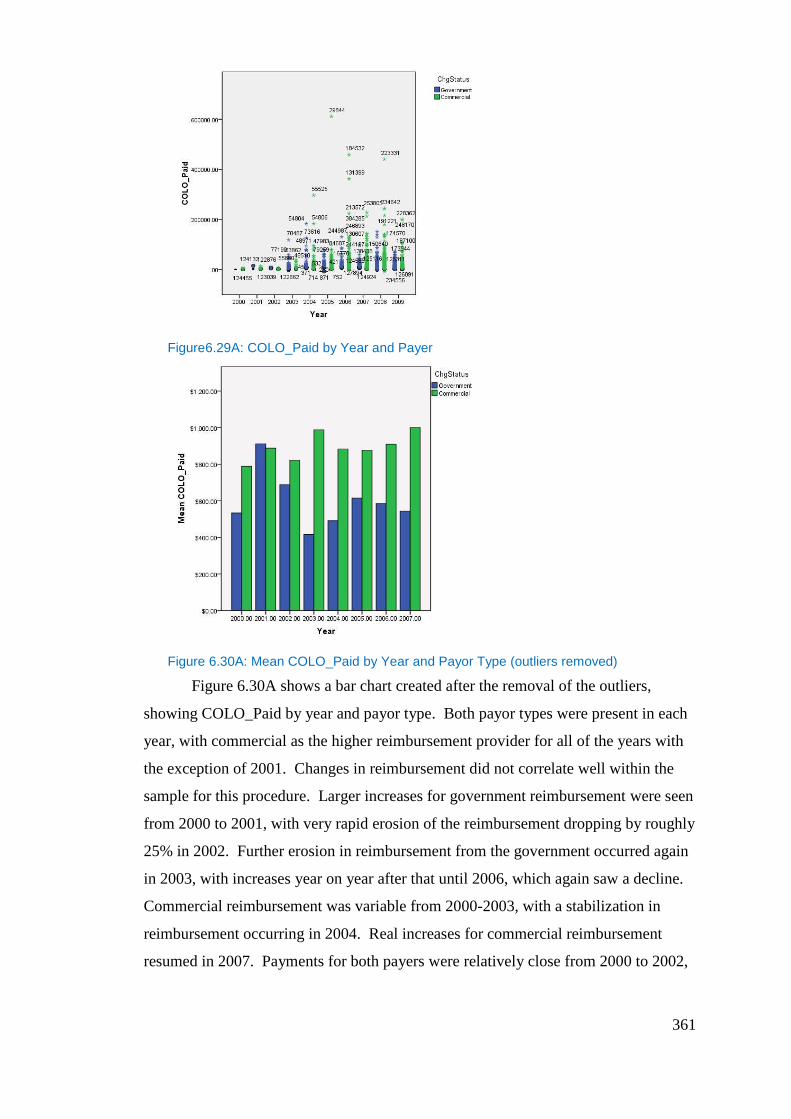
361
Figure6.29A: COLO_Paid by Year and Payer
Figure 6.30A: Mean COLO_Paid by Year and Payor Type (outliers removed)
Figure 6.30A shows a bar chart created after the removal of the outliers,
showing COLO_Paid by year and payor type. Both payor types were present in each
year, with commercial as the higher reimbursement provider for all of the years with
the exception of 2001. Changes in reimbursement did not correlate well within the
sample for this procedure. Larger increases for government reimbursement were seen
from 2000 to 2001, with very rapid erosion of the reimbursement dropping by roughly
25% in 2002. Further erosion in reimbursement from the government occurred again
in 2003, with increases year on year after that until 2006, which again saw a decline.
Commercial reimbursement was variable from 2000-2003, with a stabilization in
reimbursement occurring in 2004. Real increases for commercial reimbursement
resumed in 2007. Payments for both payers were relatively close from 2000 to 2002,

362
with a large divergence in reimbursement occurring thereafter. Commercial
reimbursement from 2002 onwards was approximately 25% to 50% more than
government in any one year. All values presented are in nominal dollars.
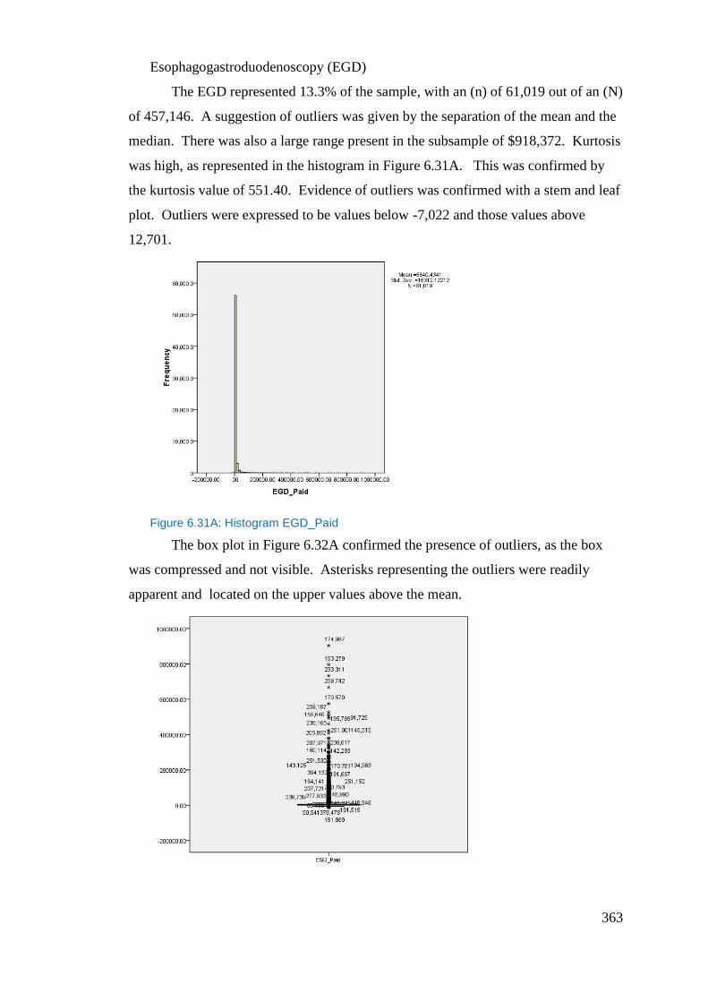
363
Esophagogastroduodenoscopy (EGD)
The EGD represented 13.3% of the sample, with an (n) of 61,019 out of an (N)
of 457,146. A suggestion of outliers was given by the separation of the mean and the
median. There was also a large range present in the subsample of $918,372. Kurtosis
was high, as represented in the histogram in Figure 6.31A. This was confirmed by
the kurtosis value of 551.40. Evidence of outliers was confirmed with a stem and leaf
plot. Outliers were expressed to be values below -7,022 and those values above
12,701.
Figure 6.31A: Histogram EGD_Paid
The box plot in Figure 6.32A confirmed the presence of outliers, as the box
was compressed and not visible. Asterisks representing the outliers were readily
apparent and located on the upper values above the mean.
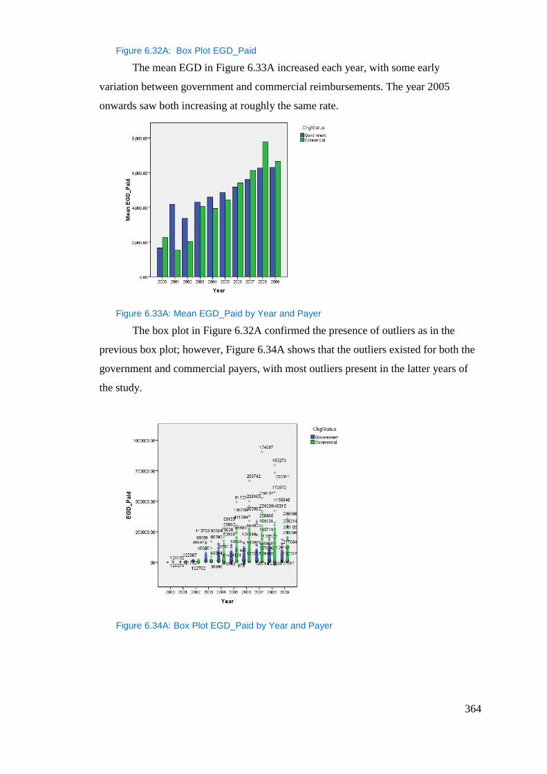
364
Figure 6.32A: Box Plot EGD_Paid
The mean EGD in Figure 6.33A increased each year, with some early
variation between government and commercial reimbursements. The year 2005
onwards saw both increasing at roughly the same rate.
Figure 6.33A: Mean EGD_Paid by Year and Payer
The box plot in Figure 6.32A confirmed the presence of outliers as in the
previous box plot; however, Figure 6.34A shows that the outliers existed for both the
government and commercial payers, with most outliers present in the latter years of
the study.
Figure 6.34A: Box Plot EGD_Paid by Year and Payer
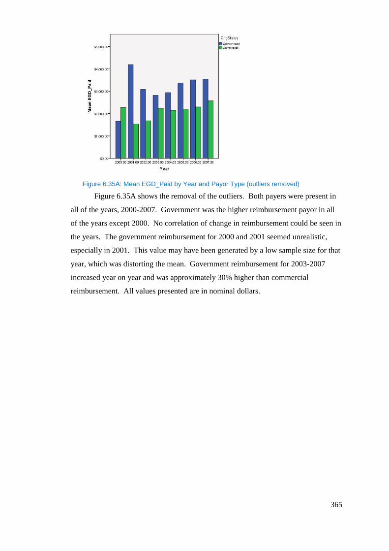
365
Figure 6.35A: Mean EGD_Paid by Year and Payor Type (outliers removed)
Figure 6.35A shows the removal of the outliers. Both payers were present in
all of the years, 2000-2007. Government was the higher reimbursement payor in all
of the years except 2000. No correlation of change in reimbursement could be seen in
the years. The government reimbursement for 2000 and 2001 seemed unrealistic,
especially in 2001. This value may have been generated by a low sample size for that
year, which was distorting the mean. Government reimbursement for 2003-2007
increased year on year and was approximately 30% higher than commercial
reimbursement. All values presented are in nominal dollars.
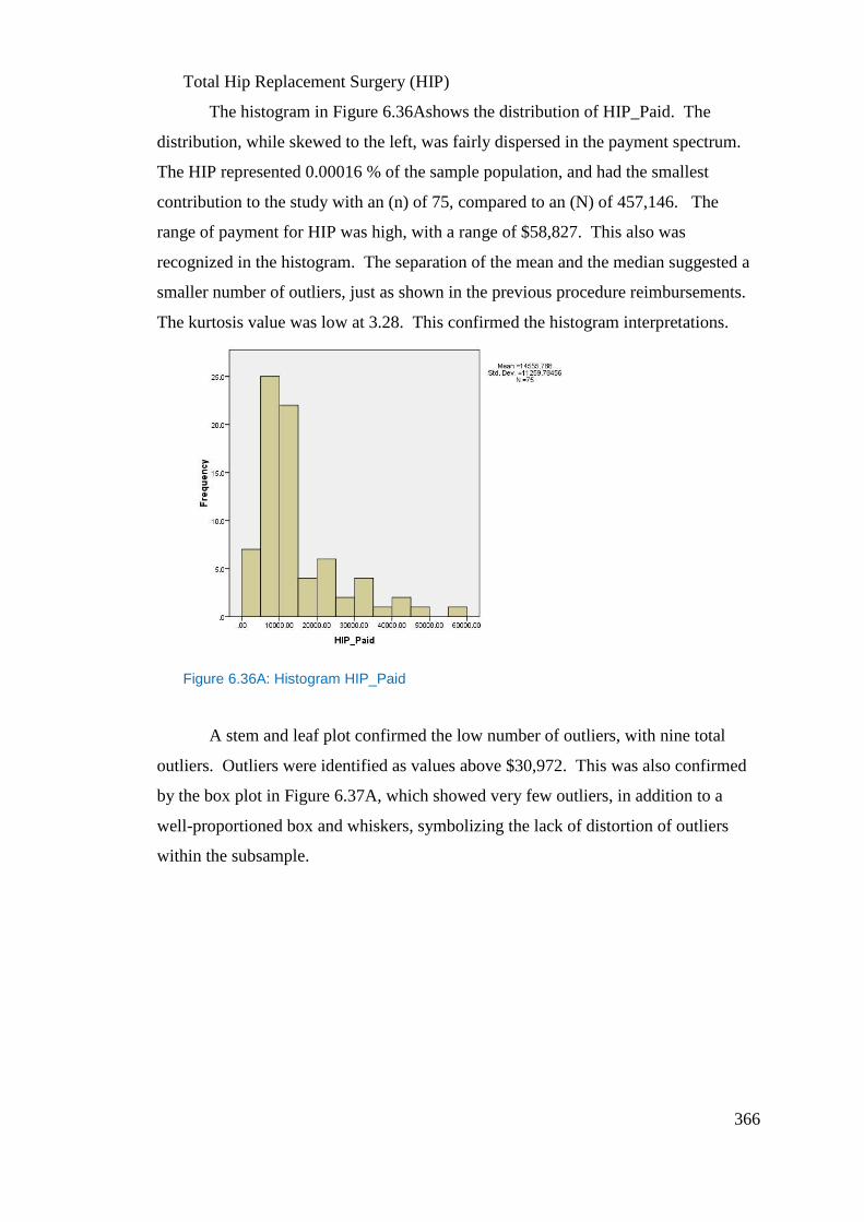
366
Total Hip Replacement Surgery (HIP)
The histogram in Figure 6.36Ashows the distribution of HIP_Paid. The
distribution, while skewed to the left, was fairly dispersed in the payment spectrum.
The HIP represented 0.00016 % of the sample population, and had the smallest
contribution to the study with an (n) of 75, compared to an (N) of 457,146. The
range of payment for HIP was high, with a range of $58,827. This also was
recognized in the histogram. The separation of the mean and the median suggested a
smaller number of outliers, just as shown in the previous procedure reimbursements.
The kurtosis value was low at 3.28. This confirmed the histogram interpretations.
Figure 6.36A: Histogram HIP_Paid
A stem and leaf plot confirmed the low number of outliers, with nine total
outliers. Outliers were identified as values above $30,972. This was also confirmed
by the box plot in Figure 6.37A, which showed very few outliers, in addition to a
well-proportioned box and whiskers, symbolizing the lack of distortion of outliers
within the subsample.
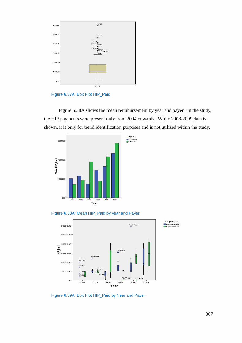
367
Figure 6.37A: Box Plot HIP_Paid
Figure 6.38A shows the mean reimbursement by year and payer. In the study,
the HIP payments were present only from 2004 onwards. While 2008-2009 data is
shown, it is only for trend identification purposes and is not utilized within the study.
Figure 6.38A: Mean HIP_Paid by year and Payer
Figure 6.39A: Box Plot HIP_Paid by Year and Payer
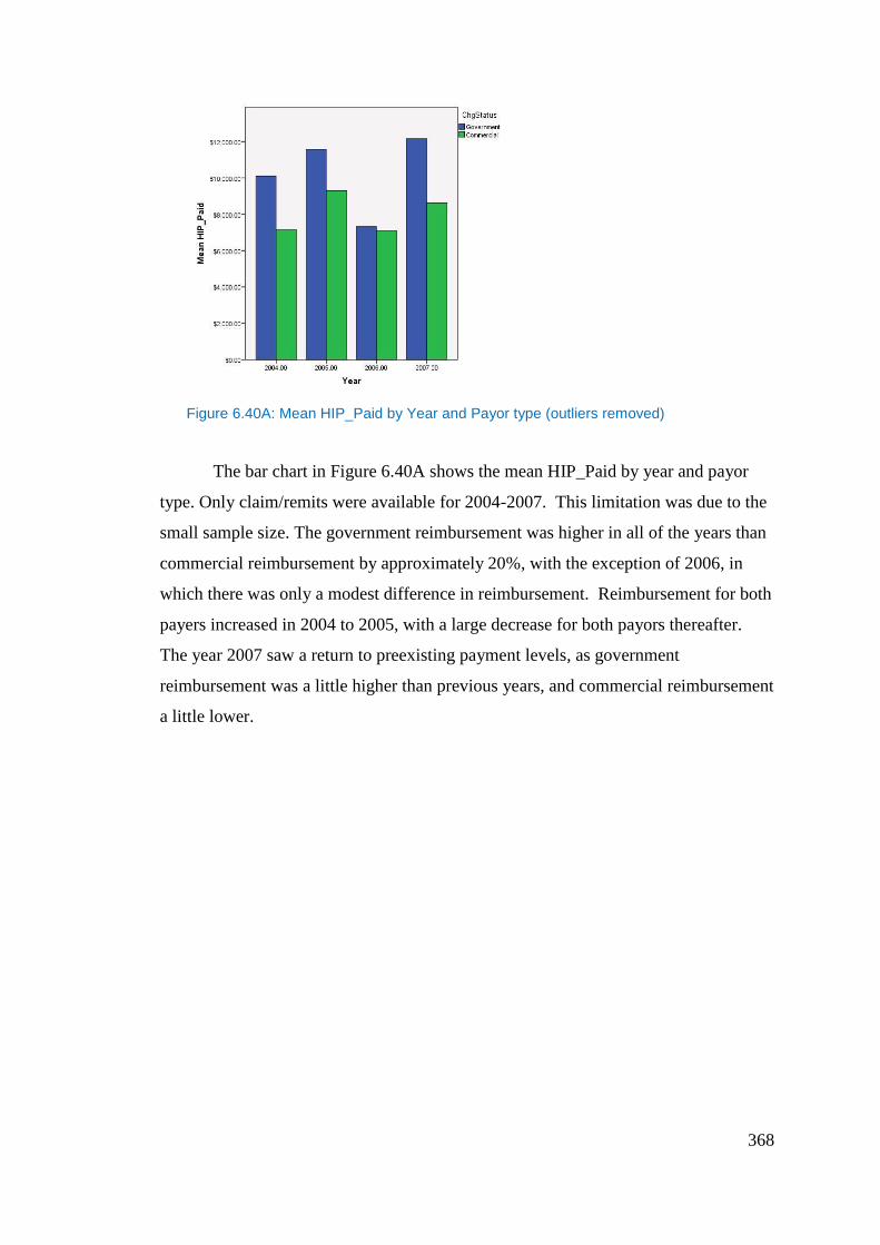
368
Figure 6.40A: Mean HIP_Paid by Year and Payor type (outliers removed)
The bar chart in Figure 6.40A shows the mean HIP_Paid by year and payor
type. Only claim/remits were available for 2004-2007. This limitation was due to the
small sample size. The government reimbursement was higher in all of the years than
commercial reimbursement by approximately 20%, with the exception of 2006, in
which there was only a modest difference in reimbursement. Reimbursement for both
payers increased in 2004 to 2005, with a large decrease for both payors thereafter.
The year 2007 saw a return to preexisting payment levels, as government
reimbursement was a little higher than previous years, and commercial reimbursement
a little lower.
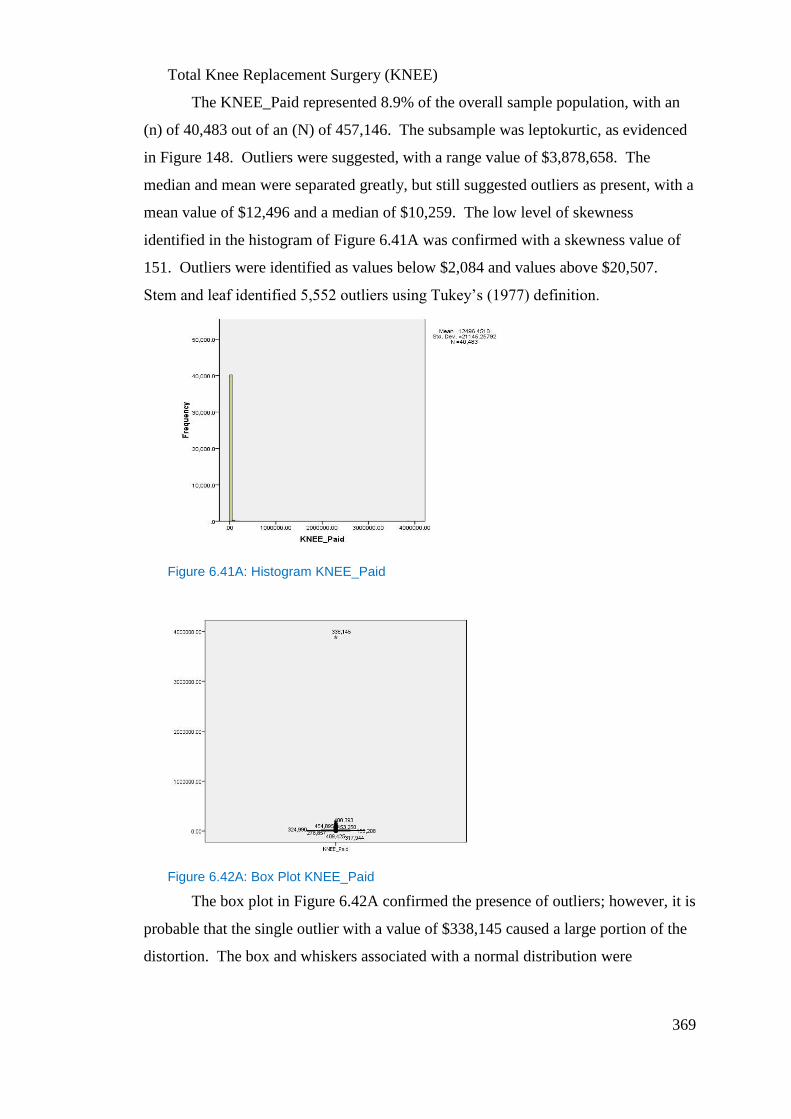
369
Total Knee Replacement Surgery (KNEE)
The KNEE_Paid represented 8.9% of the overall sample population, with an
(n) of 40,483 out of an (N) of 457,146. The subsample was leptokurtic, as evidenced
in Figure 148. Outliers were suggested, with a range value of $3,878,658. The
median and mean were separated greatly, but still suggested outliers as present, with a
mean value of $12,496 and a median of $10,259. The low level of skewness
identified in the histogram of Figure 6.41A was confirmed with a skewness value of
151. Outliers were identified as values below $2,084 and values above $20,507.
Stem and leaf identified 5,552 outliers using Tukey’s (1977) definition.
Figure 6.41A: Histogram KNEE_Paid
Figure 6.42A: Box Plot KNEE_Paid
The box plot in Figure 6.42A confirmed the presence of outliers; however, it is
probable that the single outlier with a value of $338,145 caused a large portion of the
distortion. The box and whiskers associated with a normal distribution were
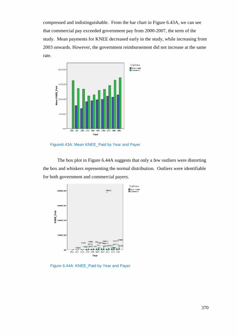
370
compressed and indistinguishable. From the bar chart in Figure 6.43A, we can see
that commercial pay exceeded government pay from 2000-2007, the term of the
study. Mean payments for KNEE decreased early in the study, while increasing from
2003 onwards. However, the government reimbursement did not increase at the same
rate.
Figure6.43A: Mean KNEE_Paid by Year and Payer
The box plot in Figure 6.44A suggests that only a few outliers were distorting
the box and whiskers representing the normal distribution. Outliers were identifiable
for both government and commercial payers.
Figure 6.44A: KNEE_Paid by Year and Payer
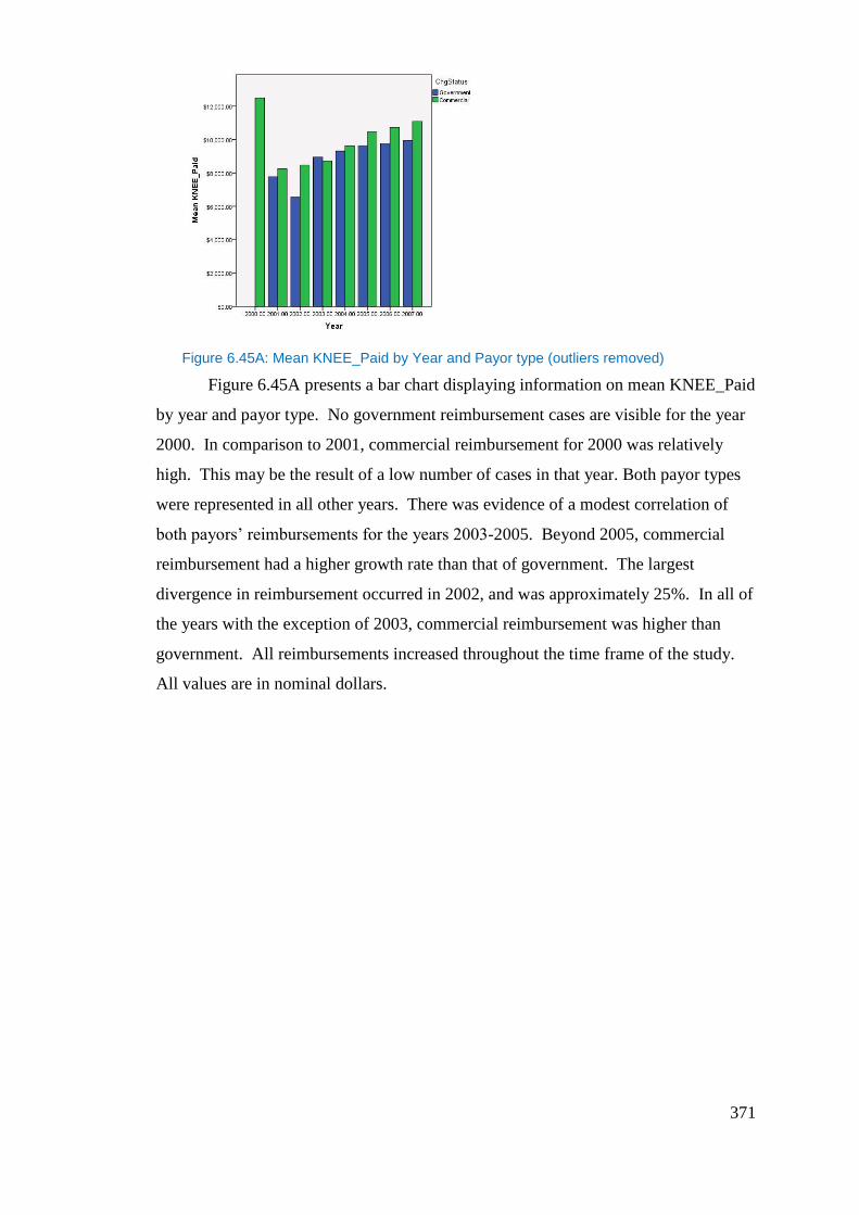
371
Figure 6.45A: Mean KNEE_Paid by Year and Payor type (outliers removed)
Figure 6.45A presents a bar chart displaying information on mean KNEE_Paid
by year and payor type. No government reimbursement cases are visible for the year
2000. In comparison to 2001, commercial reimbursement for 2000 was relatively
high. This may be the result of a low number of cases in that year. Both payor types
were represented in all other years. There was evidence of a modest correlation of
both payors’ reimbursements for the years 2003-2005. Beyond 2005, commercial
reimbursement had a higher growth rate than that of government. The largest
divergence in reimbursement occurred in 2002, and was approximately 25%. In all of
the years with the exception of 2003, commercial reimbursement was higher than
government. All reimbursements increased throughout the time frame of the study.
All values are in nominal dollars.
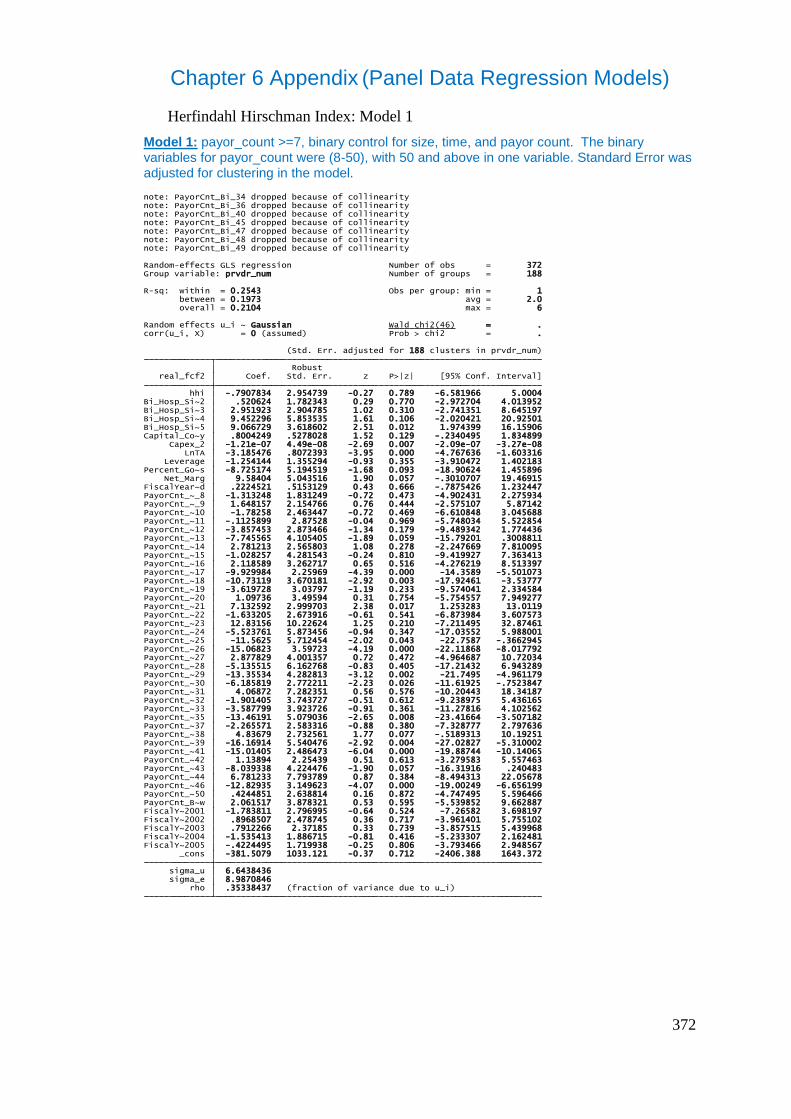
372
Chapter 6 Appendix (Panel Data Regression Models)
Herfindahl Hirschman Index: Model 1
Model 1: payor_count >=7, binary control for size, time, and payor count. The binary variables for payor_count were (8-50), with 50 and above in one variable. Standard Error was adjusted for clustering in the model.
rho .35338437 (fraction of variance due to u_i) sigma_e 8.9870846 sigma_u 6.6438436 _cons -381.5079 1033.121 -0.37 0.712 -2406.388 1643.372FiscalY~2005 -.4224495 1.719938 -0.25 0.806 -3.793466 2.948567FiscalY~2004 -1.535413 1.886715 -0.81 0.416 -5.233307 2.162481FiscalY~2003 .7912266 2.37185 0.33 0.739 -3.857515 5.439968FiscalY~2002 .8968507 2.478745 0.36 0.717 -3.961401 5.755102FiscalY~2001 -1.783811 2.796995 -0.64 0.524 -7.26582 3.698197PayorCnt_B~w 2.061517 3.878321 0.53 0.595 -5.539852 9.662887PayorCnt_~50 .4244851 2.638814 0.16 0.872 -4.747495 5.596466PayorCnt_~46 -12.82935 3.149623 -4.07 0.000 -19.00249 -6.656199PayorCnt_~44 6.781233 7.793789 0.87 0.384 -8.494313 22.05678PayorCnt_~43 -8.039338 4.224476 -1.90 0.057 -16.31916 .240483PayorCnt_~42 1.13894 2.25439 0.51 0.613 -3.279583 5.557463PayorCnt_~41 -15.01405 2.486473 -6.04 0.000 -19.88744 -10.14065PayorCnt_~39 -16.16914 5.540476 -2.92 0.004 -27.02827 -5.310002PayorCnt_~38 4.83679 2.732561 1.77 0.077 -.5189313 10.19251PayorCnt_~37 -2.265571 2.583316 -0.88 0.380 -7.328777 2.797636PayorCnt_~35 -13.46191 5.079036 -2.65 0.008 -23.41664 -3.507182PayorCnt_~33 -3.587799 3.923726 -0.91 0.361 -11.27816 4.102562PayorCnt_~32 -1.901405 3.743727 -0.51 0.612 -9.238975 5.436165PayorCnt_~31 4.06872 7.282351 0.56 0.576 -10.20443 18.34187PayorCnt_~30 -6.185819 2.772211 -2.23 0.026 -11.61925 -.7523847PayorCnt_~29 -13.35534 4.282813 -3.12 0.002 -21.7495 -4.961179PayorCnt_~28 -5.135515 6.162768 -0.83 0.405 -17.21432 6.943289PayorCnt_~27 2.877829 4.001357 0.72 0.472 -4.964687 10.72034PayorCnt_~26 -15.06823 3.59723 -4.19 0.000 -22.11868 -8.017792PayorCnt_~25 -11.5625 5.712454 -2.02 0.043 -22.7587 -.3662945PayorCnt_~24 -5.523761 5.873456 -0.94 0.347 -17.03552 5.988001PayorCnt_~23 12.83156 10.22624 1.25 0.210 -7.211495 32.87461PayorCnt_~22 -1.633205 2.673916 -0.61 0.541 -6.873984 3.607573PayorCnt_~21 7.132592 2.999703 2.38 0.017 1.253283 13.0119PayorCnt_~20 1.09736 3.49594 0.31 0.754 -5.754557 7.949277PayorCnt_~19 -3.619728 3.03797 -1.19 0.233 -9.574041 2.334584PayorCnt_~18 -10.73119 3.670181 -2.92 0.003 -17.92461 -3.53777PayorCnt_~17 -9.929984 2.25969 -4.39 0.000 -14.3589 -5.501073PayorCnt_~16 2.118589 3.262717 0.65 0.516 -4.276219 8.513397PayorCnt_~15 -1.028257 4.281543 -0.24 0.810 -9.419927 7.363413PayorCnt_~14 2.781213 2.565803 1.08 0.278 -2.247669 7.810095PayorCnt_~13 -7.745565 4.105405 -1.89 0.059 -15.79201 .3008811PayorCnt_~12 -3.857453 2.873466 -1.34 0.179 -9.489342 1.774436PayorCnt_~11 -.1125899 2.87528 -0.04 0.969 -5.748034 5.522854PayorCnt_~10 -1.78258 2.463447 -0.72 0.469 -6.610848 3.045688PayorCnt_~_9 1.648157 2.154766 0.76 0.444 -2.575107 5.87142PayorCnt_~_8 -1.313248 1.831249 -0.72 0.473 -4.902431 2.275934FiscalYear~d .2224521 .5153129 0.43 0.666 -.7875426 1.232447 Net_Marg 9.58404 5.043516 1.90 0.057 -.3010707 19.46915Percent_Go~s -8.725174 5.194519 -1.68 0.093 -18.90624 1.455896 Leverage -1.254144 1.355294 -0.93 0.355 -3.910472 1.402183 LnTA -3.185476 .8072393 -3.95 0.000 -4.767636 -1.603316 Capex_2 -1.21e-07 4.49e-08 -2.69 0.007 -2.09e-07 -3.27e-08Capital_Co~y .8004249 .5278028 1.52 0.129 -.2340495 1.834899Bi_Hosp_Si~5 9.066729 3.618602 2.51 0.012 1.974399 16.15906Bi_Hosp_Si~4 9.452296 5.853535 1.61 0.106 -2.020421 20.92501Bi_Hosp_Si~3 2.951923 2.904785 1.02 0.310 -2.741351 8.645197Bi_Hosp_Si~2 .520624 1.782343 0.29 0.770 -2.972704 4.013952 hhi -.7907834 2.954739 -0.27 0.789 -6.581966 5.0004 real_fcf2 Coef. Std. Err. z P>|z| [95% Conf. Interval] Robust (Std. Err. adjusted for 188 clusters in prvdr_num)
corr(u_i, X) = 0 (assumed) Prob > chi2 = .Random effects u_i ~ Gaussian Wald chi2(46) = .
overall = 0.2104 max = 6 between = 0.1973 avg = 2.0R-sq: within = 0.2543 Obs per group: min = 1
Group variable: prvdr_num Number of groups = 188Random-effects GLS regression Number of obs = 372
note: PayorCnt_Bi_49 dropped because of collinearitynote: PayorCnt_Bi_48 dropped because of collinearitynote: PayorCnt_Bi_47 dropped because of collinearitynote: PayorCnt_Bi_45 dropped because of collinearitynote: PayorCnt_Bi_40 dropped because of collinearitynote: PayorCnt_Bi_36 dropped because of collinearitynote: PayorCnt_Bi_34 dropped because of collinearity

373
Herfindahl Hirschman Index: Model 2
Model 2: payor_count >=6, binary control for size, time, and payor count. The binary variables for payor_count were (7-50), with 50 and above in one variable. Standard Error was adjusted for clustering in the model.
rho .34628039 (fraction of variance due to u_i) sigma_e 8.9087856 sigma_u 6.4839058 _cons -450.4745 803.9166 -0.56 0.575 -2026.122 1125.173FiscalY~2005 .7688406 1.463165 0.53 0.599 -2.09891 3.636591FiscalY~2004 -1.007094 1.561207 -0.65 0.519 -4.067004 2.052816FiscalY~2003 .1400753 1.958551 0.07 0.943 -3.698614 3.978764FiscalY~2002 .5696517 2.09207 0.27 0.785 -3.53073 4.670034FiscalY~2001 -.2308872 2.496359 -0.09 0.926 -5.123662 4.661887PayorCnt_B~w 2.074541 3.805137 0.55 0.586 -5.38339 9.532472PayorCnt_~50 1.738038 2.484988 0.70 0.484 -3.132449 6.608524PayorCnt_~46 -13.54832 3.140258 -4.31 0.000 -19.70311 -7.393525PayorCnt_~44 7.142922 7.44888 0.96 0.338 -7.456614 21.74246PayorCnt_~43 -6.227932 4.336697 -1.44 0.151 -14.7277 2.271838PayorCnt_~42 1.31608 1.970187 0.67 0.504 -2.545415 5.177576PayorCnt_~41 -15.16885 2.688445 -5.64 0.000 -20.4381 -9.899591PayorCnt_~39 -16.20656 5.835999 -2.78 0.005 -27.64491 -4.768211PayorCnt_~38 5.073881 2.819659 1.80 0.072 -.4525487 10.60031PayorCnt_~37 -1.865154 2.731862 -0.68 0.495 -7.219506 3.489198PayorCnt_~35 -13.41653 4.106737 -3.27 0.001 -21.46559 -5.367473PayorCnt_~33 -2.635527 4.178623 -0.63 0.528 -10.82548 5.554424PayorCnt_~32 -1.201851 3.466374 -0.35 0.729 -7.99582 5.592117PayorCnt_~31 5.226138 6.856835 0.76 0.446 -8.21301 18.66529PayorCnt_~30 -3.953716 2.751921 -1.44 0.151 -9.347381 1.43995PayorCnt_~29 -12.50335 3.700258 -3.38 0.001 -19.75573 -5.250982PayorCnt_~28 -4.608916 5.448305 -0.85 0.398 -15.2874 6.069566PayorCnt_~27 4.022255 3.924292 1.02 0.305 -3.669216 11.71373PayorCnt_~26 -13.30193 2.997575 -4.44 0.000 -19.17707 -7.426794PayorCnt_~25 -10.69801 5.341924 -2.00 0.045 -21.16798 -.2280274PayorCnt_~24 -5.207758 6.207737 -0.84 0.402 -17.3747 6.959182PayorCnt_~23 13.94187 9.914308 1.41 0.160 -5.489814 33.37356PayorCnt_~22 -.1569702 2.867373 -0.05 0.956 -5.776918 5.462978PayorCnt_~21 7.151199 2.69631 2.65 0.008 1.866527 12.43587PayorCnt_~20 1.043676 3.45569 0.30 0.763 -5.729353 7.816704PayorCnt_~19 -2.33376 2.857604 -0.82 0.414 -7.934562 3.267041PayorCnt_~18 -10.35763 3.479787 -2.98 0.003 -17.17789 -3.537378PayorCnt_~17 -9.115063 2.105031 -4.33 0.000 -13.24085 -4.989279PayorCnt_~16 2.493433 3.174535 0.79 0.432 -3.728541 8.715408PayorCnt_~15 -.2424922 4.130975 -0.06 0.953 -8.339054 7.85407PayorCnt_~14 2.598777 2.652206 0.98 0.327 -2.599452 7.797005PayorCnt_~13 -7.113977 4.097109 -1.74 0.083 -15.14416 .916208PayorCnt_~12 -3.101275 2.75047 -1.13 0.260 -8.492097 2.289548PayorCnt_~11 .2038708 2.661228 0.08 0.939 -5.012041 5.419782PayorCnt_~10 -.8219982 2.435224 -0.34 0.736 -5.59495 3.950954PayorCnt_~_9 2.388259 2.104629 1.13 0.256 -1.736739 6.513257PayorCnt_~_8 -1.054818 1.924334 -0.55 0.584 -4.826443 2.716808PayorCnt_~_7 .5156602 1.554173 0.33 0.740 -2.530462 3.561783FiscalYear~d .2561131 .4008228 0.64 0.523 -.5294852 1.041711 Net_Marg 9.47596 5.210856 1.82 0.069 -.7371306 19.68905Percent_Go~s -9.71394 4.648209 -2.09 0.037 -18.82426 -.6036188 Leverage -1.447085 1.185254 -1.22 0.222 -3.77014 .8759711 LnTA -3.11706 .7588358 -4.11 0.000 -4.604351 -1.629769 Capex_2 -1.47e-07 3.96e-08 -3.71 0.000 -2.25e-07 -6.93e-08Capital_Co~y 1.05756 .3936477 2.69 0.007 .2860248 1.829095Bi_Hosp_Si~5 9.249199 3.31492 2.79 0.005 2.752075 15.74632Bi_Hosp_Si~4 11.14671 5.284668 2.11 0.035 .7889481 21.50447Bi_Hosp_Si~3 3.602507 2.489165 1.45 0.148 -1.276166 8.48118Bi_Hosp_Si~2 .6874729 1.58319 0.43 0.664 -2.415522 3.790467 hhi -.8366864 2.483555 -0.34 0.736 -5.704365 4.030992 real_fcf2 Coef. Std. Err. z P>|z| [95% Conf. Interval] Robust (Std. Err. adjusted for 242 clusters in prvdr_num)
corr(u_i, X) = 0 (assumed) Prob > chi2 = .Random effects u_i ~ Gaussian Wald chi2(47) = .
overall = 0.1879 max = 6 between = 0.1716 avg = 1.9R-sq: within = 0.2206 Obs per group: min = 1
Group variable: prvdr_num Number of groups = 242Random-effects GLS regression Number of obs = 471
note: PayorCnt_Bi_49 dropped because of collinearitynote: PayorCnt_Bi_48 dropped because of collinearitynote: PayorCnt_Bi_47 dropped because of collinearitynote: PayorCnt_Bi_45 dropped because of collinearitynote: PayorCnt_Bi_40 dropped because of collinearitynote: PayorCnt_Bi_36 dropped because of collinearitynote: PayorCnt_Bi_34 dropped because of collinearity
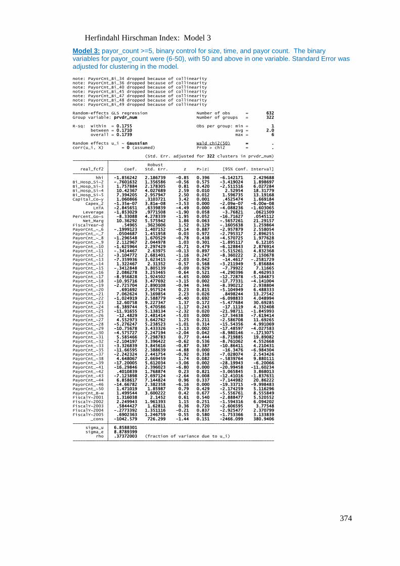
374
Herfindahl Hirschman Index: Model 3
Model 3: payor_count >=5, binary control for size, time, and payor count. The binary variables for payor_count were (6-50), with 50 and above in one variable. Standard Error was adjusted for clustering in the model.
rho .37372003 (fraction of variance due to u_i) sigma_e 8.8789399 sigma_u 6.8588301 _cons -1042.579 726.299 -1.44 0.151 -2466.099 380.9406FiscalY~2005 .6902363 1.246759 0.55 0.580 -1.753366 3.133839FiscalY~2004 -.2773392 1.351116 -0.21 0.837 -2.925477 2.370799FiscalY~2003 .5844427 1.62811 0.36 0.720 -2.606595 3.77548FiscalY~2002 2.249943 1.961393 1.15 0.251 -1.594316 6.094202FiscalY~2001 1.316038 2.1452 0.61 0.540 -2.888477 5.520552PayorCnt_B~w 1.499544 3.600222 0.42 0.677 -5.556761 8.555849PayorCnt_~50 1.471019 1.85987 0.79 0.429 -2.174259 5.116296PayorCnt_~46 -14.66782 2.382358 -6.16 0.000 -19.33715 -9.998483PayorCnt_~44 6.858617 7.144824 0.96 0.337 -7.144982 20.86222PayorCnt_~43 -7.123898 2.697124 -2.64 0.008 -12.41016 -1.837631PayorCnt_~42 .4010839 1.768874 0.23 0.821 -3.065845 3.868013PayorCnt_~41 -16.29846 2.396023 -6.80 0.000 -20.99458 -11.60234PayorCnt_~39 -17.20005 5.612034 -3.06 0.002 -28.19943 -6.20066PayorCnt_~38 4.648067 2.669459 1.74 0.082 -.5839764 9.880111PayorCnt_~37 -2.242324 2.441754 -0.92 0.358 -7.028074 2.543426PayorCnt_~35 -11.66595 2.388639 -4.88 0.000 -16.3476 -6.984304PayorCnt_~33 -3.326839 3.845616 -0.87 0.387 -10.86411 4.210431PayorCnt_~32 -2.104197 3.396422 -0.62 0.536 -8.761062 4.552668PayorCnt_~31 5.585466 7.298783 0.77 0.444 -8.719885 19.89082PayorCnt_~30 -4.575727 2.247194 -2.04 0.042 -8.980146 -.1713075PayorCnt_~29 -10.75678 3.433326 -3.13 0.002 -17.48597 -4.027583PayorCnt_~28 -5.276247 5.238523 -1.01 0.314 -15.54356 4.991069PayorCnt_~27 4.552973 3.642762 1.25 0.211 -2.586708 11.69265PayorCnt_~26 -12.4829 2.481414 -5.03 0.000 -17.34638 -7.619414PayorCnt_~25 -11.91655 5.138134 -2.32 0.020 -21.98711 -1.845993PayorCnt_~24 -6.389744 5.470586 -1.17 0.243 -17.1119 4.332408PayorCnt_~23 12.60758 9.227347 1.37 0.172 -5.477684 30.69285PayorCnt_~22 -1.024919 2.588779 -0.40 0.692 -6.098833 4.048994PayorCnt_~21 7.062624 3.169854 2.23 0.026 .8498244 13.27542PayorCnt_~20 .691692 2.957524 0.23 0.815 -5.104949 6.488333PayorCnt_~19 -2.725704 2.890108 -0.94 0.346 -8.390212 2.938804PayorCnt_~18 -10.95716 3.477692 -3.15 0.002 -17.77331 -4.141004PayorCnt_~17 -8.956828 1.924502 -4.65 0.000 -12.72878 -5.184873PayorCnt_~16 2.086278 3.253465 0.64 0.521 -4.290396 8.462953PayorCnt_~15 -.3412848 3.805139 -0.09 0.929 -7.79922 7.11665PayorCnt_~14 1.322467 2.31352 0.57 0.568 -3.211949 5.856884PayorCnt_~13 -7.359936 3.623415 -2.03 0.042 -14.4617 -.2581729PayorCnt_~12 -3.104772 2.681401 -1.16 0.247 -8.360222 2.150678PayorCnt_~11 -.3414467 2.63975 -0.13 0.897 -5.515261 4.832368PayorCnt_~10 -1.625964 2.297429 -0.71 0.479 -6.128843 2.876914PayorCnt_~_9 2.112967 2.044978 1.03 0.301 -1.895117 6.12105PayorCnt_~_8 -1.296548 1.670529 -0.78 0.438 -4.570725 1.977628PayorCnt_~_7 .0504687 1.451958 0.03 0.972 -2.795317 2.896255PayorCnt_~_6 -.1999123 1.407152 -0.14 0.887 -2.957879 2.558054FiscalYear~d .54965 .3623606 1.52 0.129 -.1605638 1.259864 Net_Marg 10.36292 5.575942 1.86 0.063 -.5657261 21.29157Percent_Go~s -8.33088 4.278339 -1.95 0.052 -16.71627 .0545112 Leverage -1.853029 .9771508 -1.90 0.058 -3.76821 .0621509 LnTA -2.845651 .6339839 -4.49 0.000 -4.088236 -1.603065 Capex_2 -1.35e-07 3.81e-08 -3.53 0.000 -2.09e-07 -6.00e-08Capital_Co~y 1.060866 .3103721 3.42 0.001 .4525474 1.669184Bi_Hosp_Si~5 7.394205 2.957947 2.50 0.012 1.596735 13.19168Bi_Hosp_Si~4 10.42367 4.027689 2.59 0.010 2.52954 18.31779Bi_Hosp_Si~3 1.757884 2.178305 0.81 0.420 -2.511516 6.027284Bi_Hosp_Si~2 -.7601632 1.356586 -0.56 0.575 -3.419024 1.898697 hhi -1.856242 2.186739 -0.85 0.396 -6.142171 2.429688 real_fcf2 Coef. Std. Err. z P>|z| [95% Conf. Interval] Robust (Std. Err. adjusted for 322 clusters in prvdr_num)
corr(u_i, X) = 0 (assumed) Prob > chi2 = .Random effects u_i ~ Gaussian Wald chi2(50) = .
overall = 0.1739 max = 6 between = 0.1710 avg = 2.0R-sq: within = 0.1755 Obs per group: min = 1
Group variable: prvdr_num Number of groups = 322Random-effects GLS regression Number of obs = 632
note: PayorCnt_Bi_49 dropped because of collinearitynote: PayorCnt_Bi_48 dropped because of collinearitynote: PayorCnt_Bi_47 dropped because of collinearitynote: PayorCnt_Bi_45 dropped because of collinearitynote: PayorCnt_Bi_40 dropped because of collinearitynote: PayorCnt_Bi_36 dropped because of collinearitynote: PayorCnt_Bi_34 dropped because of collinearity
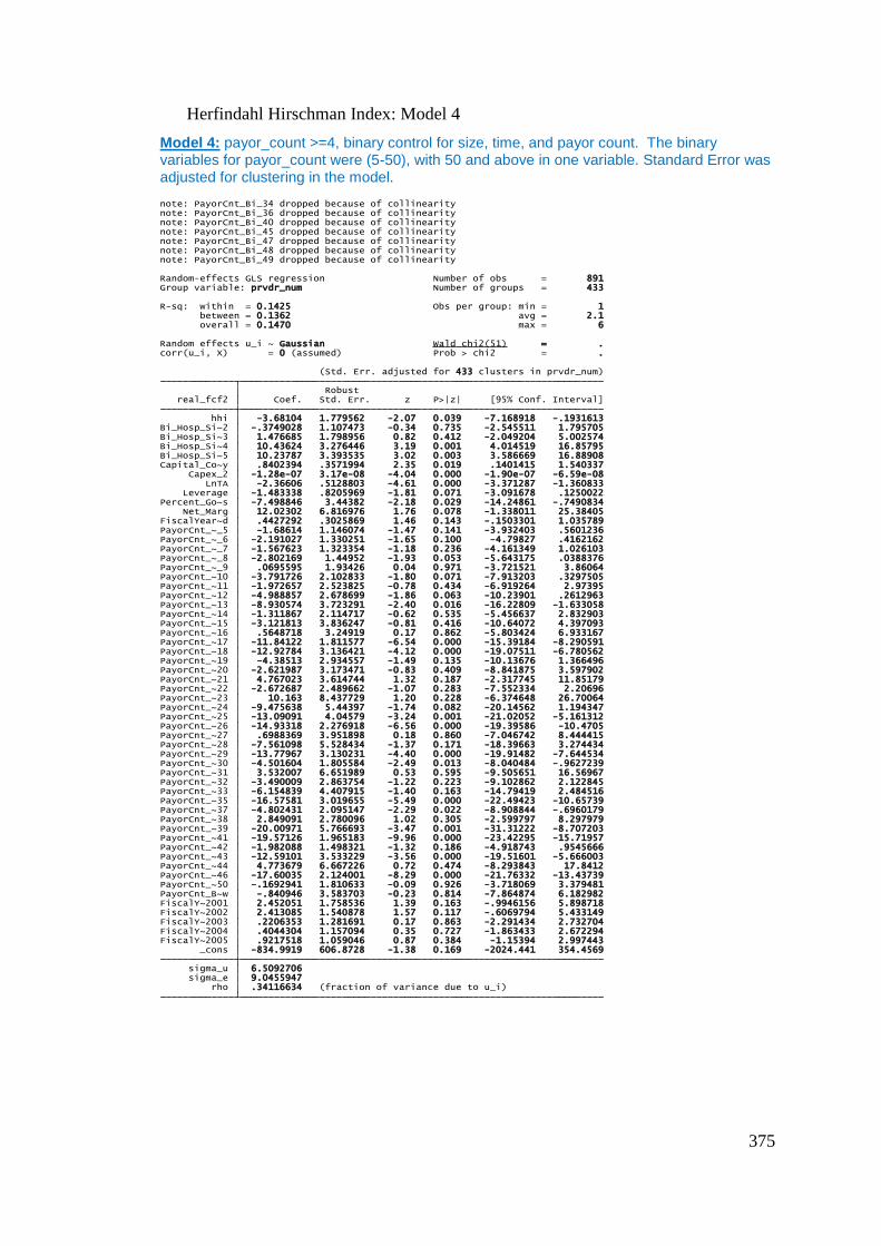
375
Herfindahl Hirschman Index: Model 4
Model 4: payor_count >=4, binary control for size, time, and payor count. The binary variables for payor_count were (5-50), with 50 and above in one variable. Standard Error was adjusted for clustering in the model.
rho .34116634 (fraction of variance due to u_i) sigma_e 9.0455947 sigma_u 6.5092706 _cons -834.9919 606.8728 -1.38 0.169 -2024.441 354.4569FiscalY~2005 .9217518 1.059046 0.87 0.384 -1.15394 2.997443FiscalY~2004 .4044304 1.157094 0.35 0.727 -1.863433 2.672294FiscalY~2003 .2206353 1.281691 0.17 0.863 -2.291434 2.732704FiscalY~2002 2.413085 1.540878 1.57 0.117 -.6069794 5.433149FiscalY~2001 2.452051 1.758536 1.39 0.163 -.9946156 5.898718PayorCnt_B~w -.840946 3.583703 -0.23 0.814 -7.864874 6.182982PayorCnt_~50 -.1692941 1.810633 -0.09 0.926 -3.718069 3.379481PayorCnt_~46 -17.60035 2.124001 -8.29 0.000 -21.76332 -13.43739PayorCnt_~44 4.773679 6.667226 0.72 0.474 -8.293843 17.8412PayorCnt_~43 -12.59101 3.533229 -3.56 0.000 -19.51601 -5.666003PayorCnt_~42 -1.982088 1.498321 -1.32 0.186 -4.918743 .9545666PayorCnt_~41 -19.57126 1.965183 -9.96 0.000 -23.42295 -15.71957PayorCnt_~39 -20.00971 5.766693 -3.47 0.001 -31.31222 -8.707203PayorCnt_~38 2.849091 2.780096 1.02 0.305 -2.599797 8.297979PayorCnt_~37 -4.802431 2.095147 -2.29 0.022 -8.908844 -.6960179PayorCnt_~35 -16.57581 3.019655 -5.49 0.000 -22.49423 -10.65739PayorCnt_~33 -6.154839 4.407915 -1.40 0.163 -14.79419 2.484516PayorCnt_~32 -3.490009 2.863754 -1.22 0.223 -9.102862 2.122845PayorCnt_~31 3.532007 6.651989 0.53 0.595 -9.505651 16.56967PayorCnt_~30 -4.501604 1.805584 -2.49 0.013 -8.040484 -.9627239PayorCnt_~29 -13.77967 3.130231 -4.40 0.000 -19.91482 -7.644534PayorCnt_~28 -7.561098 5.528434 -1.37 0.171 -18.39663 3.274434PayorCnt_~27 .6988369 3.951898 0.18 0.860 -7.046742 8.444415PayorCnt_~26 -14.93318 2.276918 -6.56 0.000 -19.39586 -10.4705PayorCnt_~25 -13.09091 4.04579 -3.24 0.001 -21.02052 -5.161312PayorCnt_~24 -9.475638 5.44397 -1.74 0.082 -20.14562 1.194347PayorCnt_~23 10.163 8.437729 1.20 0.228 -6.374648 26.70064PayorCnt_~22 -2.672687 2.489662 -1.07 0.283 -7.552334 2.20696PayorCnt_~21 4.767023 3.614744 1.32 0.187 -2.317745 11.85179PayorCnt_~20 -2.621987 3.173471 -0.83 0.409 -8.841875 3.597902PayorCnt_~19 -4.38513 2.934557 -1.49 0.135 -10.13676 1.366496PayorCnt_~18 -12.92784 3.136421 -4.12 0.000 -19.07511 -6.780562PayorCnt_~17 -11.84122 1.811577 -6.54 0.000 -15.39184 -8.290591PayorCnt_~16 .5648718 3.24919 0.17 0.862 -5.803424 6.933167PayorCnt_~15 -3.121813 3.836247 -0.81 0.416 -10.64072 4.397093PayorCnt_~14 -1.311867 2.114717 -0.62 0.535 -5.456637 2.832903PayorCnt_~13 -8.930574 3.723291 -2.40 0.016 -16.22809 -1.633058PayorCnt_~12 -4.988857 2.678699 -1.86 0.063 -10.23901 .2612963PayorCnt_~11 -1.972657 2.523825 -0.78 0.434 -6.919264 2.97395PayorCnt_~10 -3.791726 2.102833 -1.80 0.071 -7.913203 .3297505PayorCnt_~_9 .0695595 1.93426 0.04 0.971 -3.721521 3.86064PayorCnt_~_8 -2.802169 1.44952 -1.93 0.053 -5.643175 .0388376PayorCnt_~_7 -1.567623 1.323354 -1.18 0.236 -4.161349 1.026103PayorCnt_~_6 -2.191027 1.330251 -1.65 0.100 -4.79827 .4162162PayorCnt_~_5 -1.68614 1.146074 -1.47 0.141 -3.932403 .5601236FiscalYear~d .4427292 .3025869 1.46 0.143 -.1503301 1.035789 Net_Marg 12.02302 6.816976 1.76 0.078 -1.338011 25.38405Percent_Go~s -7.498846 3.44382 -2.18 0.029 -14.24861 -.7490834 Leverage -1.483338 .8205969 -1.81 0.071 -3.091678 .1250022 LnTA -2.36606 .5128803 -4.61 0.000 -3.371287 -1.360833 Capex_2 -1.28e-07 3.17e-08 -4.04 0.000 -1.90e-07 -6.59e-08Capital_Co~y .8402394 .3571994 2.35 0.019 .1401415 1.540337Bi_Hosp_Si~5 10.23787 3.393535 3.02 0.003 3.586669 16.88908Bi_Hosp_Si~4 10.43624 3.276446 3.19 0.001 4.014519 16.85795Bi_Hosp_Si~3 1.476685 1.798956 0.82 0.412 -2.049204 5.002574Bi_Hosp_Si~2 -.3749028 1.107473 -0.34 0.735 -2.545511 1.795705 hhi -3.68104 1.779562 -2.07 0.039 -7.168918 -.1931613 real_fcf2 Coef. Std. Err. z P>|z| [95% Conf. Interval] Robust (Std. Err. adjusted for 433 clusters in prvdr_num)
corr(u_i, X) = 0 (assumed) Prob > chi2 = .Random effects u_i ~ Gaussian Wald chi2(51) = .
overall = 0.1470 max = 6 between = 0.1362 avg = 2.1R-sq: within = 0.1425 Obs per group: min = 1
Group variable: prvdr_num Number of groups = 433Random-effects GLS regression Number of obs = 891
note: PayorCnt_Bi_49 dropped because of collinearitynote: PayorCnt_Bi_48 dropped because of collinearitynote: PayorCnt_Bi_47 dropped because of collinearitynote: PayorCnt_Bi_45 dropped because of collinearitynote: PayorCnt_Bi_40 dropped because of collinearitynote: PayorCnt_Bi_36 dropped because of collinearitynote: PayorCnt_Bi_34 dropped because of collinearity
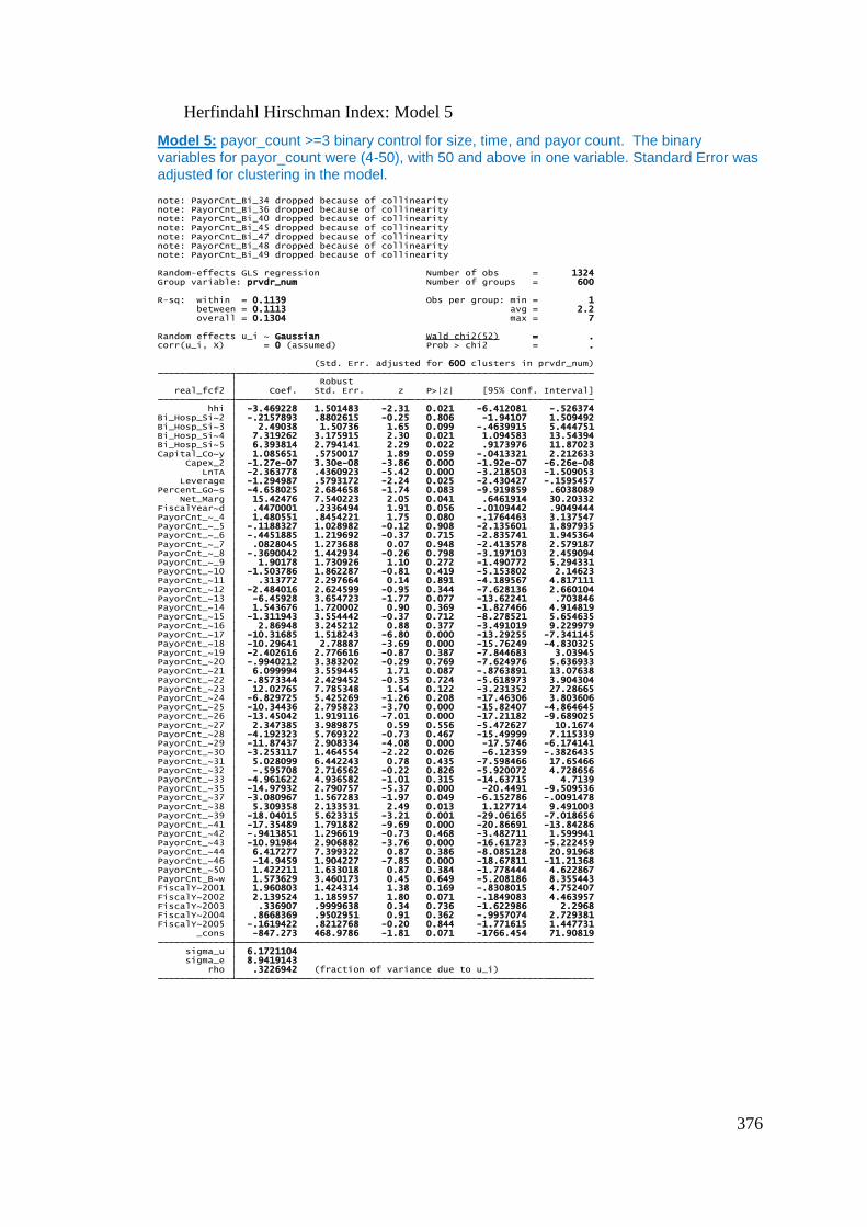
376
Herfindahl Hirschman Index: Model 5
Model 5: payor_count >=3 binary control for size, time, and payor count. The binary variables for payor_count were (4-50), with 50 and above in one variable. Standard Error was adjusted for clustering in the model.
rho .3226942 (fraction of variance due to u_i) sigma_e 8.9419143 sigma_u 6.1721104 _cons -847.273 468.9786 -1.81 0.071 -1766.454 71.90819FiscalY~2005 -.1619422 .8212768 -0.20 0.844 -1.771615 1.447731FiscalY~2004 .8668369 .9502951 0.91 0.362 -.9957074 2.729381FiscalY~2003 .336907 .9999638 0.34 0.736 -1.622986 2.2968FiscalY~2002 2.139524 1.185957 1.80 0.071 -.1849083 4.463957FiscalY~2001 1.960803 1.424314 1.38 0.169 -.8308015 4.752407PayorCnt_B~w 1.573629 3.460173 0.45 0.649 -5.208186 8.355443PayorCnt_~50 1.422211 1.633018 0.87 0.384 -1.778444 4.622867PayorCnt_~46 -14.9459 1.904227 -7.85 0.000 -18.67811 -11.21368PayorCnt_~44 6.417277 7.399322 0.87 0.386 -8.085128 20.91968PayorCnt_~43 -10.91984 2.906882 -3.76 0.000 -16.61723 -5.222459PayorCnt_~42 -.9413851 1.296619 -0.73 0.468 -3.482711 1.599941PayorCnt_~41 -17.35489 1.791882 -9.69 0.000 -20.86691 -13.84286PayorCnt_~39 -18.04015 5.623315 -3.21 0.001 -29.06165 -7.018656PayorCnt_~38 5.309358 2.133531 2.49 0.013 1.127714 9.491003PayorCnt_~37 -3.080967 1.567283 -1.97 0.049 -6.152786 -.0091478PayorCnt_~35 -14.97932 2.790757 -5.37 0.000 -20.4491 -9.509536PayorCnt_~33 -4.961622 4.936582 -1.01 0.315 -14.63715 4.7139PayorCnt_~32 -.595708 2.716562 -0.22 0.826 -5.920072 4.728656PayorCnt_~31 5.028099 6.442243 0.78 0.435 -7.598466 17.65466PayorCnt_~30 -3.253117 1.464554 -2.22 0.026 -6.12359 -.3826435PayorCnt_~29 -11.87437 2.908334 -4.08 0.000 -17.5746 -6.174141PayorCnt_~28 -4.192323 5.769322 -0.73 0.467 -15.49999 7.115339PayorCnt_~27 2.347385 3.989875 0.59 0.556 -5.472627 10.1674PayorCnt_~26 -13.45042 1.919116 -7.01 0.000 -17.21182 -9.689025PayorCnt_~25 -10.34436 2.795823 -3.70 0.000 -15.82407 -4.864645PayorCnt_~24 -6.829725 5.425269 -1.26 0.208 -17.46306 3.803606PayorCnt_~23 12.02765 7.785348 1.54 0.122 -3.231352 27.28665PayorCnt_~22 -.8573344 2.429452 -0.35 0.724 -5.618973 3.904304PayorCnt_~21 6.099994 3.559445 1.71 0.087 -.8763891 13.07638PayorCnt_~20 -.9940212 3.383202 -0.29 0.769 -7.624976 5.636933PayorCnt_~19 -2.402616 2.776616 -0.87 0.387 -7.844683 3.03945PayorCnt_~18 -10.29641 2.78887 -3.69 0.000 -15.76249 -4.830325PayorCnt_~17 -10.31685 1.518243 -6.80 0.000 -13.29255 -7.341145PayorCnt_~16 2.86948 3.245212 0.88 0.377 -3.491019 9.229979PayorCnt_~15 -1.311943 3.554442 -0.37 0.712 -8.278521 5.654635PayorCnt_~14 1.543676 1.720002 0.90 0.369 -1.827466 4.914819PayorCnt_~13 -6.45928 3.654723 -1.77 0.077 -13.62241 .703846PayorCnt_~12 -2.484016 2.624599 -0.95 0.344 -7.628136 2.660104PayorCnt_~11 .313772 2.297664 0.14 0.891 -4.189567 4.817111PayorCnt_~10 -1.503786 1.862287 -0.81 0.419 -5.153802 2.14623PayorCnt_~_9 1.90178 1.730926 1.10 0.272 -1.490772 5.294331PayorCnt_~_8 -.3690042 1.442934 -0.26 0.798 -3.197103 2.459094PayorCnt_~_7 .0828045 1.273688 0.07 0.948 -2.413578 2.579187PayorCnt_~_6 -.4451885 1.219692 -0.37 0.715 -2.835741 1.945364PayorCnt_~_5 -.1188327 1.028982 -0.12 0.908 -2.135601 1.897935PayorCnt_~_4 1.480551 .8454221 1.75 0.080 -.1764463 3.137547FiscalYear~d .4470001 .2336494 1.91 0.056 -.0109442 .9049444 Net_Marg 15.42476 7.540223 2.05 0.041 .6461914 30.20332Percent_Go~s -4.658025 2.684658 -1.74 0.083 -9.919859 .6038089 Leverage -1.294987 .5793172 -2.24 0.025 -2.430427 -.1595457 LnTA -2.363778 .4360923 -5.42 0.000 -3.218503 -1.509053 Capex_2 -1.27e-07 3.30e-08 -3.86 0.000 -1.92e-07 -6.26e-08Capital_Co~y 1.085651 .5750017 1.89 0.059 -.0413321 2.212633Bi_Hosp_Si~5 6.393814 2.794141 2.29 0.022 .9173976 11.87023Bi_Hosp_Si~4 7.319262 3.175915 2.30 0.021 1.094583 13.54394Bi_Hosp_Si~3 2.49038 1.50736 1.65 0.099 -.4639915 5.444751Bi_Hosp_Si~2 -.2157893 .8802615 -0.25 0.806 -1.94107 1.509492 hhi -3.469228 1.501483 -2.31 0.021 -6.412081 -.526374 real_fcf2 Coef. Std. Err. z P>|z| [95% Conf. Interval] Robust (Std. Err. adjusted for 600 clusters in prvdr_num)
corr(u_i, X) = 0 (assumed) Prob > chi2 = .Random effects u_i ~ Gaussian Wald chi2(52) = .
overall = 0.1304 max = 7 between = 0.1113 avg = 2.2R-sq: within = 0.1139 Obs per group: min = 1
Group variable: prvdr_num Number of groups = 600Random-effects GLS regression Number of obs = 1324
note: PayorCnt_Bi_49 dropped because of collinearitynote: PayorCnt_Bi_48 dropped because of collinearitynote: PayorCnt_Bi_47 dropped because of collinearitynote: PayorCnt_Bi_45 dropped because of collinearitynote: PayorCnt_Bi_40 dropped because of collinearitynote: PayorCnt_Bi_36 dropped because of collinearitynote: PayorCnt_Bi_34 dropped because of collinearity

377
Herfindahl Hirschman Index: Model 6
Model 6: payor_count >=2 binary control for size, time, and payor count. The binary variables for payor_count were (3-50), with 50 and above in one variable. Standard Error was adjusted for clustering in the model.
rho .31960603 (fraction of variance due to u_i) sigma_e 9.0789247 sigma_u 6.2224535 _cons -794.3081 361.6525 -2.20 0.028 -1503.134 -85.48231FiscalY~2005 .3140344 .6825318 0.46 0.645 -1.023703 1.651772FiscalY~2004 .5043008 .746121 0.68 0.499 -.9580695 1.966671FiscalY~2003 -.3361836 .7541581 -0.45 0.656 -1.814306 1.141939FiscalY~2002 1.233776 .9010122 1.37 0.171 -.5321753 2.999728FiscalY~2001 2.753071 1.029123 2.68 0.007 .7360265 4.770115PayorCnt_B~w .8178675 3.431579 0.24 0.812 -5.907904 7.543639PayorCnt_~50 .0405295 1.841856 0.02 0.982 -3.569442 3.650501PayorCnt_~46 -16.51599 1.689513 -9.78 0.000 -19.82738 -13.20461PayorCnt_~44 5.820901 7.320395 0.80 0.427 -8.52681 20.16861PayorCnt_~43 -9.844519 3.6828 -2.67 0.008 -17.06267 -2.626365PayorCnt_~42 -1.811335 1.164596 -1.56 0.120 -4.093901 .4712298PayorCnt_~41 -18.19559 1.566908 -11.61 0.000 -21.26667 -15.12451PayorCnt_~39 -19.74678 5.664866 -3.49 0.000 -30.84971 -8.643845PayorCnt_~38 4.376198 1.987516 2.20 0.028 .4807388 8.271657PayorCnt_~37 -3.729736 2.464409 -1.51 0.130 -8.559888 1.100416PayorCnt_~35 -16.09842 2.354722 -6.84 0.000 -20.71359 -11.48325PayorCnt_~33 -5.111546 5.220263 -0.98 0.327 -15.34307 5.119982PayorCnt_~32 -.2357601 2.581991 -0.09 0.927 -5.29637 4.82485PayorCnt_~31 4.159428 5.707523 0.73 0.466 -7.027112 15.34597PayorCnt_~30 -4.28706 1.349263 -3.18 0.001 -6.931566 -1.642553PayorCnt_~29 -13.02842 2.600624 -5.01 0.000 -18.12555 -7.931293PayorCnt_~28 -5.324272 4.627197 -1.15 0.250 -14.39341 3.744868PayorCnt_~27 1.758303 3.784448 0.46 0.642 -5.659078 9.175684PayorCnt_~26 -13.80567 1.716733 -8.04 0.000 -17.1704 -10.44093PayorCnt_~25 -11.05028 2.657943 -4.16 0.000 -16.25975 -5.840806PayorCnt_~24 -7.166011 6.014396 -1.19 0.233 -18.95401 4.621989PayorCnt_~23 12.09672 7.622352 1.59 0.113 -2.842812 27.03626PayorCnt_~22 -1.237881 2.242157 -0.55 0.581 -5.632429 3.156667PayorCnt_~21 5.609239 3.577598 1.57 0.117 -1.402725 12.6212PayorCnt_~20 -2.604937 3.517756 -0.74 0.459 -9.499612 4.289737PayorCnt_~19 -2.876996 2.739945 -1.05 0.294 -8.24719 2.493198PayorCnt_~18 -11.36945 2.931735 -3.88 0.000 -17.11554 -5.623354PayorCnt_~17 -11.27527 1.470685 -7.67 0.000 -14.15776 -8.39278PayorCnt_~16 1.882334 3.150051 0.60 0.550 -4.291652 8.056321PayorCnt_~15 -2.276258 3.677803 -0.62 0.536 -9.484621 4.932104PayorCnt_~14 .3869989 1.778249 0.22 0.828 -3.098304 3.872302PayorCnt_~13 -7.031105 3.463672 -2.03 0.042 -13.81978 -.2424331PayorCnt_~12 -3.440894 2.655737 -1.30 0.195 -8.646043 1.764255PayorCnt_~11 -.8499334 1.992054 -0.43 0.670 -4.754287 3.054421PayorCnt_~10 -2.473704 1.881198 -1.31 0.189 -6.160784 1.213375PayorCnt_~_9 1.151586 1.730659 0.67 0.506 -2.240443 4.543615PayorCnt_~_8 -1.105027 1.464367 -0.75 0.450 -3.975132 1.765079PayorCnt_~_7 -.9846462 1.255808 -0.78 0.433 -3.445984 1.476692PayorCnt_~_6 -1.213739 1.157262 -1.05 0.294 -3.481931 1.054453PayorCnt_~_5 -.8767582 1.009993 -0.87 0.385 -2.856307 1.102791PayorCnt_~_4 .7039098 .7504156 0.94 0.348 -.7668777 2.174697PayorCnt_~_3 -.7944862 .6149912 -1.29 0.196 -1.999847 .4108744FiscalYear~d .4197049 .1803349 2.33 0.020 .0662551 .7731547 Net_Marg 22.02755 8.467436 2.60 0.009 5.431683 38.62342Percent_Go~s -4.015043 2.302029 -1.74 0.081 -8.526937 .4968509 Leverage -.5695055 .4799009 -1.19 0.235 -1.510094 .371083 LnTA -2.281873 .3415583 -6.68 0.000 -2.951315 -1.612431 Capex_2 -1.59e-07 3.43e-08 -4.64 0.000 -2.27e-07 -9.19e-08Capital_Co~y .9500599 .5076786 1.87 0.061 -.0449718 1.945092Bi_Hosp_Si~5 3.886303 3.412474 1.14 0.255 -2.802023 10.57463Bi_Hosp_Si~4 7.153569 2.722199 2.63 0.009 1.818156 12.48898Bi_Hosp_Si~3 3.102911 1.240283 2.50 0.012 .6720017 5.533821Bi_Hosp_Si~2 .1470463 .7125235 0.21 0.836 -1.249474 1.543567 hhi -2.730321 1.302367 -2.10 0.036 -5.282913 -.177728 real_fcf2 Coef. Std. Err. z P>|z| [95% Conf. Interval] Robust (Std. Err. adjusted for 847 clusters in prvdr_num)
corr(u_i, X) = 0 (assumed) Prob > chi2 = .Random effects u_i ~ Gaussian Wald chi2(52) = .
overall = 0.1120 max = 7 between = 0.0886 avg = 2.5R-sq: within = 0.1075 Obs per group: min = 1
Group variable: prvdr_num Number of groups = 847Random-effects GLS regression Number of obs = 2118
note: PayorCnt_Bi_49 dropped because of collinearitynote: PayorCnt_Bi_48 dropped because of collinearitynote: PayorCnt_Bi_47 dropped because of collinearitynote: PayorCnt_Bi_45 dropped because of collinearitynote: PayorCnt_Bi_40 dropped because of collinearitynote: PayorCnt_Bi_36 dropped because of collinearitynote: PayorCnt_Bi_34 dropped because of collinearity> FiscalYear_Bi_2003 FiscalYear_Bi_2004 FiscalYear_Bi_2005, re vce(cluster prvdr_num)

378
Herfindahl Hirschman Index: Model 7
Model 7: payor_count >=1 binary control for size, time, and payor count. The binary variables for payor_count were (2-50), with 50 and above in one variable. Standard Error was adjusted for clustering in the model.
rho .25533037 (fraction of variance due to u_i) sigma_e 9.2708149 sigma_u 5.4285936 _cons -368.4784 242.412 -1.52 0.128 -843.5973 106.6404FiscalY~2005 .9084199 .5480397 1.66 0.097 -.1657182 1.982558FiscalY~2004 .7243343 .5626771 1.29 0.198 -.3784925 1.827161FiscalY~2003 .2185834 .555177 0.39 0.694 -.8695436 1.30671FiscalY~2002 .8640418 .620855 1.39 0.164 -.3528116 2.080895FiscalY~2001 1.469391 .6327748 2.32 0.020 .2291753 2.709607PayorCnt_B~w .3219108 3.425352 0.09 0.925 -6.391656 7.035478PayorCnt_~50 -.6303428 2.007579 -0.31 0.754 -4.565125 3.30444PayorCnt_~46 -15.31294 1.426433 -10.74 0.000 -18.1087 -12.51718PayorCnt_~44 5.265068 7.247503 0.73 0.468 -8.939777 19.46991PayorCnt_~43 -9.453109 4.411611 -2.14 0.032 -18.09971 -.8065105PayorCnt_~42 -2.35852 .9475945 -2.49 0.013 -4.215771 -.5012687PayorCnt_~41 -17.46933 1.233328 -14.16 0.000 -19.88661 -15.05205PayorCnt_~39 -19.3586 5.440825 -3.56 0.000 -30.02242 -8.694781PayorCnt_~38 4.138105 2.188148 1.89 0.059 -.1505857 8.426796PayorCnt_~37 -3.892487 2.390762 -1.63 0.103 -8.578294 .7933202PayorCnt_~35 -17.18462 1.994532 -8.62 0.000 -21.09384 -13.27541PayorCnt_~33 -5.921308 6.057179 -0.98 0.328 -17.79316 5.950546PayorCnt_~32 .0860434 2.145022 0.04 0.968 -4.118122 4.290209PayorCnt_~31 3.204792 4.886873 0.66 0.512 -6.373304 12.78289PayorCnt_~30 -4.095672 1.213186 -3.38 0.001 -6.473474 -1.717871PayorCnt_~29 -15.70899 2.274833 -6.91 0.000 -20.16758 -11.2504PayorCnt_~28 -6.258881 4.796827 -1.30 0.192 -15.66049 3.142728PayorCnt_~27 1.034251 3.954578 0.26 0.794 -6.716579 8.785081PayorCnt_~26 -13.76232 1.55347 -8.86 0.000 -16.80707 -10.71758PayorCnt_~25 -10.92357 2.908792 -3.76 0.000 -16.6247 -5.222444PayorCnt_~24 -6.636527 6.459553 -1.03 0.304 -19.29702 6.023964PayorCnt_~23 12.53385 8.12399 1.54 0.123 -3.388879 28.45657PayorCnt_~22 -1.473535 2.240974 -0.66 0.511 -5.865763 2.918694PayorCnt_~21 5.51943 3.794629 1.45 0.146 -1.917905 12.95677PayorCnt_~20 -1.98451 3.894976 -0.51 0.610 -9.618522 5.649503PayorCnt_~19 -3.690554 2.699331 -1.37 0.172 -8.981145 1.600037PayorCnt_~18 -11.38905 2.672264 -4.26 0.000 -16.6266 -6.151514PayorCnt_~17 -12.40509 1.325356 -9.36 0.000 -15.00274 -9.807439PayorCnt_~16 1.817993 3.000647 0.61 0.545 -4.063166 7.699153PayorCnt_~15 -2.11841 3.640458 -0.58 0.561 -9.253576 5.016757PayorCnt_~14 .5879253 1.939563 0.30 0.762 -3.213548 4.389398PayorCnt_~13 -6.342086 3.558726 -1.78 0.075 -13.31706 .6328885PayorCnt_~12 -3.425387 2.524934 -1.36 0.175 -8.374166 1.523392PayorCnt_~11 -1.198571 2.109234 -0.57 0.570 -5.332594 2.935452PayorCnt_~10 -2.497127 1.7619 -1.42 0.156 -5.950389 .9561342PayorCnt_~_9 1.491006 1.751595 0.85 0.395 -1.942057 4.924069PayorCnt_~_8 -1.164051 1.442162 -0.81 0.420 -3.990636 1.662535PayorCnt_~_7 -1.011645 1.253705 -0.81 0.420 -3.468862 1.445572PayorCnt_~_6 -1.431907 1.214966 -1.18 0.239 -3.813196 .9493825PayorCnt_~_5 -.9996961 1.020951 -0.98 0.327 -3.000723 1.001331PayorCnt_~_4 .5241562 .7714336 0.68 0.497 -.9878259 2.036138PayorCnt_~_3 -1.040766 .6037075 -1.72 0.085 -2.224011 .1424786PayorCnt_~_2 -.2881746 .4902564 -0.59 0.557 -1.249059 .6727102FiscalYear~d .2060823 .1209313 1.70 0.088 -.0309386 .4431033 Net_Marg 22.11875 6.168397 3.59 0.000 10.02891 34.20859Percent_Go~s -5.301605 1.735829 -3.05 0.002 -8.703768 -1.899442 Leverage -.6644917 .4207146 -1.58 0.114 -1.489077 .1600938 LnTA -2.102105 .2642452 -7.96 0.000 -2.620016 -1.584194 Capex_2 -1.74e-07 3.05e-08 -5.71 0.000 -2.34e-07 -1.14e-07Capital_Co~y .7571171 .4975404 1.52 0.128 -.2180441 1.732278Bi_Hosp_Si~5 4.29351 3.078214 1.39 0.163 -1.739679 10.3267Bi_Hosp_Si~4 6.388939 2.080755 3.07 0.002 2.310734 10.46714Bi_Hosp_Si~3 2.801098 .9932411 2.82 0.005 .8543812 4.747815Bi_Hosp_Si~2 .4140993 .5592943 0.74 0.459 -.6820973 1.510296 hhi -2.819972 1.254893 -2.25 0.025 -5.279517 -.3604268 real_fcf2 Coef. Std. Err. z P>|z| [95% Conf. Interval] Robust (Std. Err. adjusted for 1243 clusters in prvdr_num)
corr(u_i, X) = 0 (assumed) Prob > chi2 = .Random effects u_i ~ Gaussian Wald chi2(53) = .
overall = 0.1001 max = 7 between = 0.0964 avg = 2.8R-sq: within = 0.0747 Obs per group: min = 1
Group variable: prvdr_num Number of groups = 1243Random-effects GLS regression Number of obs = 3503
note: PayorCnt_Bi_49 dropped because of collinearitynote: PayorCnt_Bi_48 dropped because of collinearitynote: PayorCnt_Bi_47 dropped because of collinearitynote: PayorCnt_Bi_45 dropped because of collinearitynote: PayorCnt_Bi_40 dropped because of collinearitynote: PayorCnt_Bi_36 dropped because of collinearitynote: PayorCnt_Bi_34 dropped because of collinearity> iscalYear_Bi_2003 FiscalYear_Bi_2004 FiscalYear_Bi_2005, re vce(cluster prvdr_num)> ayorCnt_Bi_47 PayorCnt_Bi_48 PayorCnt_Bi_49 PayorCnt_Bi_50 PayorCnt_Bi_Other_New FiscalYear_Bi_2001 FiscalYear_Bi_2002 F> ayorCnt_Bi_39 PayorCnt_Bi_40 PayorCnt_Bi_41 PayorCnt_Bi_42 PayorCnt_Bi_43 PayorCnt_Bi_44 PayorCnt_Bi_45 PayorCnt_Bi_46 P> ayorCnt_Bi_31 PayorCnt_Bi_32 PayorCnt_Bi_33 PayorCnt_Bi_34 PayorCnt_Bi_35 PayorCnt_Bi_36 PayorCnt_Bi_37 PayorCnt_Bi_38 P> ayorCnt_Bi_23 PayorCnt_Bi_24 PayorCnt_Bi_25 PayorCnt_Bi_26 PayorCnt_Bi_27 PayorCnt_Bi_28 PayorCnt_Bi_29 PayorCnt_Bi_30 P> ayorCnt_Bi_15 PayorCnt_Bi_16 PayorCnt_Bi_17 PayorCnt_Bi_18 PayorCnt_Bi_19 PayorCnt_Bi_20 PayorCnt_Bi_21 PayorCnt_Bi_22 P> 6 PayorCnt_Bi_7 PayorCnt_Bi_8 PayorCnt_Bi_9 PayorCnt_Bi_10 PayorCnt_Bi_11 PayorCnt_Bi_12 PayorCnt_Bi_13 PayorCnt_Bi_14 P> e Percent_Gov_Business Net_Marg FiscalYear_Reported PayorCnt_Bi_2 PayorCnt_Bi_3 PayorCnt_Bi_4 PayorCnt_Bi_5 PayorCnt_Bi_. xtreg real_fcf2 hhi Bi_Hosp_Size_2 Bi_Hosp_Size_3 Bi_Hosp_Size_4 Bi_Hosp_Size_5 Capital_Cost_Proxy Capex_2 LnTA Leverag

379
Lerner’s Index: Model 1
Model 1: DV= Lerner’s Index IV= Real FCF
Binary control for size and time. Standard Error was adjusted for clustering in the model.
Lerner’s Index Model 2
Model 2: DV= Lerner’s Index IV= Net Income from Services to Patients
Binary control for size and time. Standard Error was adjusted for clustering in the model.
rho .40184127 (fraction of variance due to u_i) sigma_e 34.346331 sigma_u 28.151361 _cons 1711.312 2714.653 0.63 0.528 -3609.311 7031.935FiscalY~2005 1.404589 3.300931 0.43 0.670 -5.065117 7.874295FiscalY~2004 .8560525 3.797454 0.23 0.822 -6.586821 8.298926FiscalY~2003 -5.84609 4.49839 -1.30 0.194 -14.66277 2.970593FiscalY~2002 -3.083524 5.904363 -0.52 0.601 -14.65586 8.488815FiscalY~2001 1.560297 9.763459 0.16 0.873 -17.57573 20.69633FiscalYear~d -.8164543 1.355821 -0.60 0.547 -3.473814 1.840905 Net_Marg 120.0879 24.02219 5.00 0.000 73.00528 167.1705Percent_Go~s 1.362973 11.7487 0.12 0.908 -21.66406 24.39001 Leverage .031512 1.941936 0.02 0.987 -3.774613 3.837636 LnTA -4.133715 1.977951 -2.09 0.037 -8.010427 -.2570026 Capex_2 -3.04e-07 1.29e-07 -2.35 0.019 -5.58e-07 -5.08e-08Capital_Co~y .7287221 6.387819 0.11 0.909 -11.79117 13.24862Bi_Hosp_Si~5 161.795 82.78411 1.95 0.051 -.4588348 324.0489Bi_Hosp_Si~4 -33.41622 13.25473 -2.52 0.012 -59.39502 -7.437424Bi_Hosp_Si~3 -8.280589 6.171817 -1.34 0.180 -20.37713 3.815949Bi_Hosp_Si~2 1.414423 3.945032 0.36 0.720 -6.317698 9.146544 li -.0427535 .009118 -4.69 0.000 -.0606245 -.0248824 real_fcf2 Coef. Std. Err. z P>|z| [95% Conf. Interval] Robust (Std. Err. adjusted for 453 clusters in prvdr_num)
corr(u_i, X) = 0 (assumed) Prob > chi2 = 0.0000Random effects u_i ~ Gaussian Wald chi2(17) = 145.80
overall = 0.2325 max = 7 between = 0.2383 avg = 2.8R-sq: within = 0.1611 Obs per group: min = 1
Group variable: prvdr_num Number of groups = 453Random-effects GLS regression Number of obs = 1254
> _Bi_2002 FiscalYear_Bi_2003 FiscalYear_Bi_2004 FiscalYear_Bi_2005, re vce(cluster prvdr_num)> apex_2 LnTA Leverage Percent_Gov_Business Net_Marg FiscalYear_Reported FiscalYear_Bi_2001 FiscalYear. xtreg real_fcf2 li Bi_Hosp_Size_2 Bi_Hosp_Size_3 Bi_Hosp_Size_4 Bi_Hosp_Size_5 Capital_Cost_Proxy C
rho .74895433 (fraction of variance due to u_i) sigma_e 14.535562 sigma_u 25.106324 _cons 96.55552 1532.167 0.06 0.950 -2906.437 3099.548FiscalY~2005 .3397996 1.308645 0.26 0.795 -2.225097 2.904696FiscalY~2004 1.476432 2.061085 0.72 0.474 -2.563221 5.516085FiscalY~2003 .3996427 2.446591 0.16 0.870 -4.395588 5.194873FiscalY~2002 .6661878 3.126132 0.21 0.831 -5.460919 6.793294FiscalY~2001 .8914405 3.58207 0.25 0.803 -6.129287 7.912168FiscalYear~d -.0479383 .7643484 -0.06 0.950 -1.546034 1.450157 Net_Marg 223.1625 48.27511 4.62 0.000 128.545 317.78Percent_Go~s 5.396817 6.776293 0.80 0.426 -7.884473 18.67811 Leverage -1.013522 1.495551 -0.68 0.498 -3.944748 1.917705 LnTA -.4059566 .9876097 -0.41 0.681 -2.341636 1.529723 Capex_2 -1.07e-07 4.81e-08 -2.23 0.026 -2.01e-07 -1.30e-08Capital_Co~y -.2136986 1.98724 -0.11 0.914 -4.108618 3.681221Bi_Hosp_Si~5 -121.1134 124.365 -0.97 0.330 -364.8644 122.6375Bi_Hosp_Si~4 -10.66408 8.077534 -1.32 0.187 -26.49576 5.167596Bi_Hosp_Si~3 5.617467 2.907799 1.93 0.053 -.0817148 11.31665Bi_Hosp_Si~2 -.2099495 1.412734 -0.15 0.882 -2.978857 2.558958 li .0039882 .0016261 2.45 0.014 .000801 .0071754 net_income~2 Coef. Std. Err. z P>|z| [95% Conf. Interval] Robust (Std. Err. adjusted for 454 clusters in prvdr_num)
corr(u_i, X) = 0 (assumed) Prob > chi2 = 0.0000Random effects u_i ~ Gaussian Wald chi2(17) = 82.53
overall = 0.2776 max = 7 between = 0.2649 avg = 2.8R-sq: within = 0.3249 Obs per group: min = 1
Group variable: prvdr_num Number of groups = 454Random-effects GLS regression Number of obs = 1269
> ter prvdr_num)> Year_Bi_2001 FiscalYear_Bi_2002 FiscalYear_Bi_2003 FiscalYear_Bi_2004 FiscalYear_Bi_2005, re vce(clus> _5 Capital_Cost_Proxy Capex_2 LnTA Leverage Percent_Gov_Business Net_Marg FiscalYear_Reported Fiscal. xtreg net_income_from_svc_to_patients2 li Bi_Hosp_Size_2 Bi_Hosp_Size_3 Bi_Hosp_Size_4 Bi_Hosp_Size

380