205-1

Geostatistical Reservoir Characterization of McMurray Formation by 2-D Modeling

Weishan Ren, Oy Leuangthong and Clayton V. Deutsch

Department of Civil & Environmental Engineering,

University of Alberta

Abstract

This paper presents a 2-D geostatistical modeling method to characterize the reservoir quality for an area of the McMurray formation. Different maps are generated to reveal different aspects of reservoir properties. Trend maps and prior maps are used to understand each variable independently. Correlation matrices and the likelihood maps are used to understand the correlation between the variables and to show the predictive information contained in secondary structural data. The Bayesian updating method is used to generate a model containing the information from the well data and the secondary data. Sequence stratigraphy, petrophysical well log, and seismic data can be integrated in the modeling. The local uncertainty is accessed by the 2-D models, and the P10, P50, and P90 maps provide information on heterogeneity and uncertainty. Global uncertainty must be assessed by simulation. Examples are shown.

Introduction

The McMurray formation bears one of largest oil sands deposit in the world. A small portion of oil sands can be recovered by surface mining; however, most of bitumen reserve will be produced by advanced heavy oil recovery technology such as the Steam Assisted Gravity Drainage (SAGD) process. Several oil sands recovery projects are underway in the McMurray formation. Reservoir characterization of McMurray formation is very important for the success of those projects. The “Guide to SAGD Reservoir Characterization Using Geostatistics” prepared by the CCG in April of 2003 was followed to construct the models illustrated in this paper. This paper adds some implementation details and another example of modeling the McMurray formation.

A major contribution of geostatistics is the construction of 2-D maps with an associated measure of uncertainty. Full 3-D modeling of heterogeneity is useful; however, the advantages of using the 2-D geostatistical modeling are (1) it can provide a best estimate at locations without wells, (2) it also provides uncertainty at each location, (3) it is simpler and faster than the 3-D modeling, and especially useful in modeling a very large area where the complex 3-D geostatistical models may not be practical. This paper demonstrates the application of 2-D geostatistical modeling to characterize the bitumen reservoir in the McMurray formation.

This paper will show some results that are loosely based on a recent case study. Only a few of the wells will be used, only some of the variables will be shown, a subset of the area will be shown, and the units have been altered. The contribution of this paper is in the verification of the applicability of modern geostatistical methodology.

Several reservoir parameters are crucial for screening a reservoir for applying SAGD. The thickness of net pay or net continuous bitumen thickness (NCB) is related to the height of the

205-2

steam chamber and is very important. The bulk oil weight (BOW) measures the quality of bitumen in a formation. It is the fraction of the bitumen weight in the total rock weight. The porosity (φ) and oil saturation (1-Sw) over the net continuous bitumen are related to the recoverable bitumen by the SAGD process. An important feature of many areas of the McMurray is the presence of top water and top gas that can provide a sink for the injected steam and adversely affect recovery. These upper units are sometimes referred to as thief zones for the injected steam. Each project and company identifies different critical parameters. The typical project will involve predicting 20 to 30 variables at each 2-D location. Only a few variables will be described in this review paper. Most of the data is derived from well logs and core data.

The available data variables are divided into two types: primary variables that we must predict and secondary variables that are fairly well established and that can be used to constrain the prediction at unsampled locations. The secondary variables are primarily structural variables that are mapped from well data and seismic data (if available). The structure of McMurray formation can be inferred from well logs, sequence stratigraphy and seismic data. Three structural surfaces will be used in this paper: (1) the bottom surface of the McMurray formation (BSM), (2) the top surface of the McMurray formation (TSM), and (3) the Wabiskaw-McMurray surface (WMS), which is a maximum flooding surface above the McMurray formation. These structural data are usually quite reliable because they are the fundamental variables for all geological models, and they are usually derived from a variety of different sources. Therefore, these three variables and the calculated gross thickness (GTM) of the McMurray are treated as independent secondary variables for the 2-D modeling.

The synthetic data represents a 10,000m by 15,000m area. Each well has many variables, but we show four independent secondary data and four commonly used dependent variables (Table 1). A resolution of 100m by 100m is used for all the maps.

Table 1: Summary of the data for 2-D modeling

Secondary Data Reservoir Quality Parameters

1 2 3 4 5 6 7 8

BSM TSM WMS GTM NCB BOW φ Sw

Methodology of 2-D modeling

To model a variable with information from the variable itself and from the secondary data, the data of each variable need to be transformed into a standard normal or Gaussian distribution. The mathematical calculations are all performed using the normal scores. The final results are back transformed to original units. The methodology is adopted from S. Zanon and C.V. Deutsch’s paper from last year’s CCG Report. The following procedure is used to build a 2-D multiGaussian model:

1. Build a prior model by the kriging of the normal score dependent variables. It is a Gaussian distribution defined by y*

k and σ2K (the mean and variance).

2. Establish an N by N matrix of correlation coefficients from N variables that are each univariate Gaussian. The matrix of correlation coefficients is symmetric, that is, ρij=ρji. The diagonal elements are ρii=1 for standard Gaussian variables. The correlation

205-3

coefficients are calculated directly from available data. The more data available the better informed the correlation coefficients.

3. Calculate the multivariate likelihood model by using the correlation matrix and secondary data. The likelihood distribution is defined by the estimate y*

L and the variance σ2L.

These values define all of the information carried in all secondary data regarding the variable being predicted. Consider n secondary data, which are normal scores, yi, i=1,…,n. Using the correlation coefficients between the secondary variables and between the secondary variable and the predict variable, the weights λj, j=1,…,n can be calculated by solving the n by n system of linear equations:

, ,01

1, ,n

j i j ij

i nλ ρ ρ=

= =∑ i … (1)

The estimate of likelihood is given exactly by a weighted linear estimator:

*

1

n

L i ii

y yλ=

= ∑ i (2)

And the variance of the likelihood:

2,0

1

1n

L i ii

σ λ ρ=

= − ∑ i (3)

4. Update the prior distribution with the likelihood distribution by using the Bayesian updating method. The final distribution is a non-standard Gaussian distribution defined by the mean y and variance σ2.

* * * *

* *(1 )( 1) 1L K K L

L K

y yy σ σσ σ

+=

− − + (4)

* *

2* *(1 )( 1) 1

K L

L K

σ σσσ σ

=− − +

(5)

5. Back transform the final distribution to real units. The back transformation is non-linear, so the mean cannot be back transformed directly. Quantiles can be back transformed with no bias, therefore, the back transform of the final distribution requires transforming a large number of quantiles. The mean and variance in real units can be calculated using these transformed quantiles.

2-D mapping

During the multivariate statistical modeling, five types of maps are generated for each reservoir parameter. The trend map is used to reveal the large scale trend in each parameter. The prior map is the kriging map of each parameter after being transformed to a Gaussian variable. These two maps are created for understanding each parameter independently. A correlation matrix plots the correlation between the variables. Based on the correlations, the likelihood map is created

205-4

with the secondary data. The correlation matrix and the likelihood map provide information for understanding the correlation between the variables. Then, the Bayesian updating approach is applied to merge the prior models and likelihood models. This approach is similar to collocated cokriging, and is implemented in the Gaussian space. The updated model contains the information from well data and from secondary data. The updated map shows the results of Bayesian updating in the Gaussian space. The updated Gaussian distributions must be back transformed to real units and are often summarized by the final maps, which are the P10/P50/P90 maps of each parameter or the probability maps of these reservoir quality parameters at certain threshold.

Trend Maps

The trend map is used to provide the overall trend of each variable in the entire study area. This map is created by simple kriging with a variogram designed to reveal large scale features. Usually, a long range variogram with modest nugget effect is used. All reservoir parameters are mapped with this trend variogram. As an example, the trend maps of the NCB and BOW are shown in Figure 1. Some high value zones are shown in the left of the study area for NCB.

Prior Maps

The prior model is also created by kriging but with the data in Gaussian space and the variogram calculated and fit from the data. Therefore, the well data need to be transformed to a standard normal distribution (normal scores values) before the kriging. With the normal score data, the variogram can be calculated. Variogram maps are helpful to find the direction of continuity in each parameter. Then, it can be used to calculate the variogram of each parameter.

The experimental variograms are modeled using a semi-automatic variogram fitting algorithm. The variogram and the model of the NCB are shown in Figure 2.

Kriging was then performed using these variogram models and the normal score data. The prior model is generated with an uncertainty distribution at each location. The uncertainty is a nonstandard normal distribution with kriged mean and variance. The map of the kriged mean is the prior map. The prior map for the NCB and BOW are also shown in Figure 1. They look similar to their trend maps but have more detailed small scale features. The values on these maps are only conditional to surrounding data of the same type; we still must consider the secondary data.

Correlation Matrix and Likelihood Maps

The cross plot of each pair of the variables should be plotted to check the data and determine the correlation between the pair of variables. Problem data should be reviewed and perhaps eliminated to obtain a more representative correlation between the variables. The final correlation coefficients are summarized and shown in a correlation matrix (Figure 3).

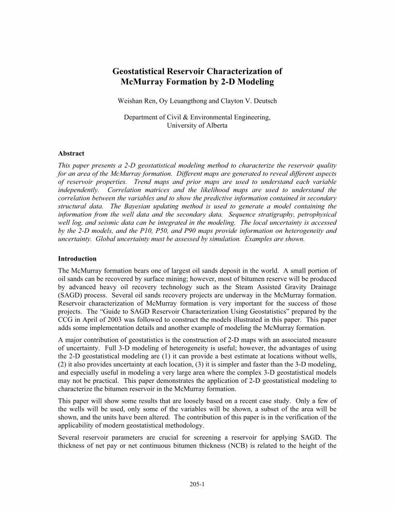
With the correlations between a reservoir parameter and the independent variables, we can use the secondary data to calculate the likelihood for these reservoir parameters. The four variables used for the secondary data are shown in Figure 4. The likelihood model provides a conditional distribution of each variable at each location conditional to collocated data of other types. The likelihood results are mapped to show the information from the secondary data. The likelihood maps of NCB and BOW are shown in Figure 5.

205-5

Updated Maps and Final Maps

The Bayesian updating is used to merge the prior models and likelihood models. The resulting model is called the updated model. The uncertainty of each parameter at each location is generated from the information of well data and the secondary data. The uncertainty distribution is also a nonstandard normal distribution with updated mean and variance. The updated map shows the updated means in Gaussian space. The updated maps of NCB and BOW are also shown in Figure 5.

The updated distribution needs to be transformed to real units to show the best estimate and the uncertainty at each location in real values. Usually, these features are summarized by P10, P50 and P90 values. The final maps show the three values of each reservoir parameter. The P50 values provide estimates of each reservoir parameter at each location. We also consider the P10 and P90 values at those locations. The P10 values provide a conservative estimate because there is a 90% probability of being larger than this value. The P10 map can also be used to identify the high value areas because when the P10 value is high then the value is surely high. The P90 values provide an optimistic estimate because there is a 90% probability of being less than this value. The P90 map can be used to identify the low valued areas because when the P90 value is low then the value is surely low.

All variables are predicted. The P10, P50 and P90 maps for NCB are shown in the Figure 6. The green color in the P10 map shows where there is a 90% chance to have more than 25 meters of net continuous bitumen. The blue color in the P90 map shows where there is a 90% chance to be less than 20 meters of net continuous bitumen.

Validation

Reservoir modeling consists of many interdependent modeling steps with ample opportunity for mistakes. It is impossible to completely validate models; however, there are some basic checks that can be used to identify problem data or errors in the geostatistical modeling. Cross validation is used to estimate the variables at locations where we know the true value. The actual data are deleted one at a time and re-estimated from the remaining neighboring wells. Then, we can check the accuracy of the predicted distributions of uncertainty to evaluate the goodness of modeling parameters.

All well locations were used for cross validation. Likelihood calculations and updating were performed. Cross validation was performed with the Gaussian transforms of the original variables. The results were back transformed to original units.

Figure 7 shows the accuracy plots of the NCB and BOW. In the accuracy plot, the points on the 45o line means that the model is both accurate and precise. If the points fall above the line, the model is accurate but not precise. If the points fall below the line, the model is neither accurate nor precise. Figure 7 shows that the model for NCB is accurate and precise.

A number of wells were drilled after these models were constructed. The goodness of the probabilistic estimates can be checked and compared to the new drilled wells. The results are shown in Figure 8. The model for NCB worked out extremely well.

205-6

Joint Uncertainty

The uncertainty at small scale (100m by 100m) is represented by distributions of uncertainty in all of the variables used to calculate the OOIP and categorize the reservoir by economic viability and/or thief zone type. The steps described above permit the calculation of uncertainty in each variable; however, there are two aspects of joint uncertainty that require simulation:

• The uncertainty in derived variables such as the OOIP (simple equation below) requires a combination of the uncertainty in the multiple (three in this case) variables. Simulation is required to combine the correlated uncertainty in constituent variables into uncertainty in the OOIP variable.

OOIP = 6.29 x 104 • NCB • φnet • So

• There is interest in the recoverable bitumen resource over large areas such as a lease boundary or pad location. Local uncertainty, as described above cannot simply be added up to obtain the joint uncertainty over larger scales.

Different techniques are required to assess multivariate uncertainty at a location and to assess global uncertainty over large volumes.

Accounting for the correlation between NCB, φ, and So is done with LU simulation. Multiple realizations (say 100) of the three variables are drawn accounting for the correlation between the variables (see yellow shaded squares in the table below). Then, the OOIP is calculated with each set of numbers. The uncertainty in the OOIP (or any other derived property) can be assembled from the realizations. A schematic table is shown below. Each set of three numbers (in yellow) is drawn by LU simulation using, for example, the LUSIM program from GSLIB.

Realization Number NCB φnet So Calculated

OOIP

1 10 0.30 0.85 160000 bbl

2 9 0.28 0.82 130000 bbl

… … … … …

100 11 0.27 0.83 155000 bbl

The LU method (named after the Cholesky LU matrix decomposition method) has been around for a long time and is suitable when the problem is small. The use of the LU method to simulate multiple dependent variables is straightforward. Only the correlation matrix between the three variables is required, and a set of correlated normal scores is required to account for the spatial correlation of the variables. The latter requirement is easily satisfied by generating unconditional realizations using sequential Gaussian simulation for each of the three variables. The procedure to calculate the LU simulation results is as follows:

The simulated value ys can be obtained by

sy w= L i

205-7

where L is the lower matrix of the correlation matrix, and w is the correlated normal scores.

Obtain the non-standardized simulated values using the updated mean and variance for each variable.

ns sy y σ µ= +i

where σ and µ are the standard deviation and mean, respectively, from the updated 2D mapping results.

Back transform the final simulated value to original units.

Assessing global uncertainty over a large area requires drawing values of each variable simultaneously over many grid nodes. There is correlation between the different variables (as described above) and spatial correlation between the variables. The LU method could also be used to model this joint multivariate and spatial correlation; however, the number of variables and locations is too large. For this reason, a P-field simulation technique is used for the spatial simulation (see the PFSIM program in GSLIB). The key idea is to simulate a set of spatially correlated probability values and then simultaneously draw the variable of interest at multiple locations. Uncertainty in larger areas is assembled from the sets of realizations.

This provides a reasonable assessment of joint uncertainty; however, uncertainty in the input parameters is not considered in this analysis. A technique such as the spatial bootstrap (see paper 401 in this report for more details) could be used to assess uncertainty in the input parameters.

Conclusion

A 2-D geostatistical modeling process is demonstrated to characterize the reservoir quality of the McMurray formation. Many different maps were created to reveal different aspects of the reservoir properties and their uncertainty. Trend maps and prior maps can be used to understand the variability of the reservoir parameter independent of any secondary information. The likelihood maps can be used to show the information from the secondary data. The updated maps contain the information from the well data as well as from the secondary data. The local uncertainty is accessed by the 2-D models, and the P10, P50, and P90 maps provide heterogeneity and uncertainty information on the bitumen reservoir properties. Moreover, the global uncertainty can be assessed by post process methods.

References

C.V. Deutsch and A.G. Journel, GSLIB: Geostatistical Software Library and User’s Guide, Oxford University Press, New York, 1998

J. McLennan and C.V. Deutsch, Guide to SAGD Reservoir Characterization Using Geostatistics, Center for Computational Geostatistics, University of Alberta, Edmonton, Alberta, April 2003

S. Zanon and C.V. Deutsch. Reservoir Performance Predicted with Multiple Geological, Geophysical, and Engineering Variables. In Center for Computational Geostatistics Report Five, University of Alberta, Edmonton, Alberta, September 2003..

205-8

Figure 1: The trend maps of NCB and BOW are shown on the top, and the Prior maps are shown on the bottom.

205-9

Figure 2: The variogram models of NCB and BOW.

205-10

Figure 3: The correlation matrix of the 11 variables

Figure 4: The maps of the four secondary data

205-11

Figure 5: The likelihood maps (top) and the updated maps (bottom) of NCB and BOW.

205-12

Figure 6: The final maps of NCB and BOW

205-13

Figure 7: The accuracy plots of cross validation results for NCB and BOW.

205-14

Figure 8: Accuracy plot of 2-D model vs. new wells