geostatistical analysis and scaling of grapevine root ... · geostatistical analysis and scaling of...

Geostatistical Analysis and Scaling of Grapevine Root Distribution

A.W. Linsenmeier, 0. Löhnertz and R. Lehnart

Forschungsanstalt Geisenheim, Fachgebiet Bodenkunde und Pflanzenernahrung, von Lade Strasse 1, D-65366 Geisenheim, Gennany

Submitted for publication: March 2011 Accepted for publication: July 2011

Key words: Fractal dimension, geostatistics, root distribution, spatial analysis, variogram, vitis

Geostatistical analysis was conducted for the root distribution of Vitis berlandieri x Vitis riparia using dispersion index, fractal dimension, autocorrelation and semivariance. The data were derived from the observation of roots of six 12-year old Riesllng/5C vine plants in a field experiment using minirhizothron technique. The dispersion index (DI) indicated the clustering of roots. Autocorrelation as a function of the distance lag showed that a higher DI was related to higher autocorrelation at small lags. Small scale (<3cm) spatial analysis using variograms, showed a clustering of roots at short distances (<6cm), but also a periodicity at greater distances (16cm) with hole effects in the variograms. The spatial variance for small scale was 60-85% within a range of 5-8cm. At medium scale (5-10cm) the spatial variance decreased to 0-20%. Geostatistical analysis is a useful tool to demonstrate variation in root distribution at plant level and to improve root sampling. Although the different geostatistical tools were related, it was not possible to deduce one result from the other quantitatively.

Abbreviations: RLD - root length density, DI— dispersion index, D - fractal dimension, mrss - minimum residual sum of squares

INTRODUCTION Roots are known to have high variability.(Smit et al., 2000). When quantitative estimates of root parameters are required, a high number of replicates are necessary to increase precision in measurement. Recently scientists have begun to investigate the source of variation instead of seeing it as a nuisance (Bengough et al., 2000). Accordingly, geostatistic techniques can be used to study the spatial variations of roots. Matheron (1965) established the theory of regionalized variables in the minery context and as a result introduced quantitative geostatistical methods. In contrast to classical statistics, variance is calculated as a function of the distance between measurement points, rather than a scalar variance. This function is called an experimental variogram. A mathematical function, called a model variogram can be applied to this experimental variogram. Using the model variogram, the radius of influence of environmental variability (range) can be determined and variance can be divided into random (nugget) and spatially-related (sill) components. Knowledge about spatial variability can be used to predict values for unknown locations by using algorithms where unknown points in the neighbourhood of the sampled points are weighted according to their distance and autocorrelation. Furthermore it can help to optimize sampling. These methods were first used in geology studies, but have recently also been applied in ecology and in plant and soil science (Dahiya et al., 1984; Böttcher and Strebel, 1988; Aiken et al., 1991;

Jackson and Caldwell, 1993). Nevertheless, studies on root distribution using variograms are extremely rare. Stoyan et al. (2000) calculated variograms for poplar and wheat root weight, Vamerali et al. (2008) used this method for maize hybrids and Scatollin et al. (2008) examined the spatial distribution of vital root tips of spruce.

Another popular tool in geostatistics is the fractal dimension, introduced by Mandelbrot (1983) and used in his pioneering work for the fractal theory in the seventies. With the fractal dimension, natural objects with non integer dimension can be described. This method is used in different fields such as economy, agronomy and environmental science, to characterise plant variety according to leaf form (Manusco, 1999) and even root distribution (Van Noordwijk et al., 1994; Nielsen et al., 1999; Salas et al., 2004).

Further geostatistic methods used in this study were autocorrelation and dispersion. In this project, vitis root observation was carried out in a field experiment using minirhizotron techniques. Results concerning dynamics in vilis root patterns were published in Lehnart et al. (2008). The degree and scale of variability in root distribution were analysed. The original data set with a fine granularity of one root length density (RLD) observation per 1.35cm was modified to coarser granularity with one RLD value per 2.70, 5.40 and 10.80cm soil layer respectively to investigate scaling effects. Furthermore, the

* Corresponding author: [email protected]

S. Afr. J. Enol. Vitic., Vol. 32, No. 2,2011 211

Geostatistics of Root Disfribution 212

relations among the parameters for spatial analysis were examined.

The aim of this work was to provide a preliminary geostatistical analysis of vitis root distribution at single plant scale, especially considering that the technique is underused in root research. Root length density (RLD) is considered as one of the best parameters related to water and nutrition uptake (Böhm, 1979). For modelling water uptake, the knowledge of RLD distribution is important, especially for non-regular root distribution because the difference in the water potential between root and soil increases with root clumping (Tardieu, 1988b, Tardieu, 1994). Geostatistical analysis can help to better describe root distribution and to improve sampling data by better estimates of unsampled regions.

MATERJALS AND METHODS Experimental designs The field experiment was carried out in April 1996 in the Rheingau, Gennany, (50°N, 8°E) in a vineyard of Vilis vinfera Riesling grapevines on 5C (Vitis berlandieri x Vilis riparia) rootstock planted in 1988. Spacing was of 2.5m2 between vine plants with perinanent green cover in every row. During root observation the areas around the vine plants were kept weed free mechanically. The soil was loamy sand with a pH of 7.4. Investigations were conducted on six vine plants labelled "A", "-I_a", "" , "D", "E" and "F".

Minirhizotron root observations Clear acrylic minirhizotron tubes with an external diameter of 6cm were used. Three 130cm long tubes were inserted for each plant: one vertically, one at an angle of 60° to the soil surface and one at an angle of 450 Roots were observed with a camera which could be advanced with increments of 1.35cm. Root observations were made with the camera facing the vine and from a perpendicular perspective. The number ofroots in the observation rectangle was converted to root length density (RLD). More details of the minirhizotron method used in this trial are given in Linsenmeier et al. (2010). The original data set with 76 observations per minirhizotron transect was modified by combining 2,4 and 8 neighbouring values. Thus resulting in RLD values for then 1.35cm (origin), 2.70cm, 5.40cm and 10.80cm layers.

Geostatistics The classical statistic tests assume that each datum is independent of all the other data. This assumption often is not true for spatial data. Geostatistical tools describe how data are related.

The concept of autocorrelation is derived from the concept of correlation of two variables in classical statistics. Autocorrelation was calculated as the correlation of the values of a single variable for all pairs separated by a distance h (Dale et al., 2002).

Dispersion is a concept describing spatial arrangement. There are three alternative models: (a) a random pattern occurs when observations are independent of each other. (b) Clumped dispersion means that an observation increases the probability of another observation in the neighbourhood. (c) When the presence of an observation decreases the

probability of finding another one nearby, the pattern is called overdispersed (or regular). The dispersion index (DI) of the root number observations was calculated as variance-to-mean ratio (see equation [1] below), sometimes also called the Fango index. With DI, the spatial pattern can be categorized as random (DI=1), clumped (DI>1) or overdispersed (DI<1) (Dale et al., 2002).

DI = CY

J_t [1]

Regionalized variable theory considers differences between data pairs separated by a distance vector h (lag h). For geostatistical analysis the assumption of stationarity has to be considered, which means that the variance between two points is the same everywhere and does not depend on the position. This is not true for root distribution. In this experiment a spatial trend can be found which on average is a quadratic function (Fig. 2). Before calculating the variograms, this spatial trend was removed by subtracting the RLD value of the regression from the corresponding original RLD value. As a consequence, the mean for the transformed data set was constant for all soil depths (stationarity), while the variance especially for higher lag distance, was smaller compared to the original data set. Semivariance was calculated according to equation [2] below, where z(x 1) is the observed RLD at position x1 and m(h) is the number of data pairs z(x 1), z(xl+h) separated by the distance h. As variance is half the square of the difference (equation [2]), the quantity y(h) was called semivariance. Nevertheless y(h) is the variance and represents the degree of statistical independence between data pairs.

1 1 m(h) 2

r(h)= m(h) Lz(xi)-z(xi+h)1 j=1 [2]

The graph of semivariance versus lag h is called an experimental variogram or semivariogram. A mathematical model called the model variogram can be fitted to the curve up to range a (Dutter, 1985). With this model variogram nugget variance, spatial variance and the range can be found (Fig.4). The nugget variance C O is the theoretical variance of two observations at a distance of 0 cm. This is due to RLD variance at the same place, or more exactly to spatial variation that occurs at distances smaller than the sampling distance, and measurement or experimental errors. The range a is the lag distance, where two points show the highest variance. Points situated at a shorter distance than the range show spatial dependence. The sill C is the maximum variance due to distance (range a) and the difference between sill and nugget variance (C-0 0) is the portion of the variance due to spatial effects. C-0 0 is zero when there is no spatial structure. When there is no sill because the semivariogram is unbound, there is usually a spatial trend (Bengough et al., 2000). Due to the modified data set, the smallest observation distance h was 1.35cm for the original data set and 2.70cm, 5.40cm and 10.80cm for the combined data set. Semivariance was calculated for each of the six observation

S. Afr. J. EnoL Vitic., VoL 32, No. 2,2011

RLD [cm/cm3 ]

0.0 0.5 1.0 1.5 2.0

DI

a 20 • ab 3.3

ab 2.7

_ 40> \ • bc 4.6 E

•A bcd 4.8

60 A• cd 67 A cd 7.5

Cn 80 - A cd 6.0

d A79

100 AED A bcd 5.2 • A ab 7.6

7 120

AC AD oE •F —Mean ......Regr

Geostatistics ofRoot Disfribution 213

0

10

20

30

40

e 50

Go 60

70

80

90

100

RLD [cm/cm3]

0 1 2 3 4 5 6

3 S -

-

o o In(r)

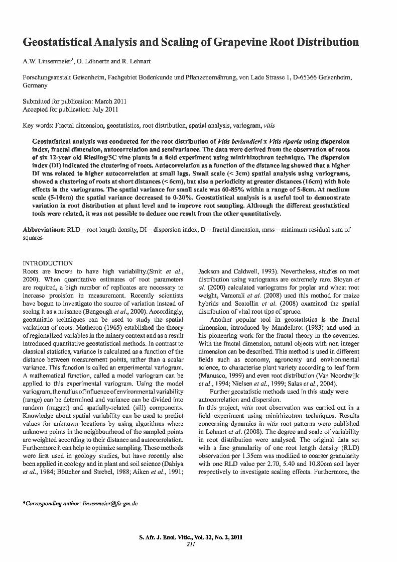
FIGURE 1 Mean root length density (RLD) of six minirhizotron

observation transects of vine plant "A" in soil depth 0-100 cm with the grid (here: r=2) used for the box counting

method. Small figure: Intersects N(r) according to the box counting method for vine plant "A", as a function of the

side length of the boxes: 2/r cm/cm 3 for RLD and 20/r cm for the soil depth respectively.

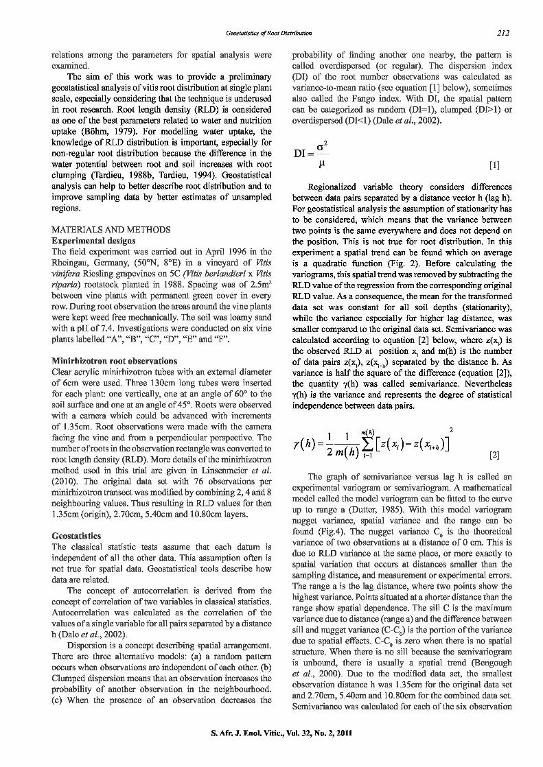
FIGURE 2 Root length density (RLD) of the six vines ("A"-"F"), mean and quadratic regression (Regr) and dispersion index (DI) in soil depth 0-120cm. For each vine the values of the six

minirhizotron observation transects have been combined to soil layers of 10cm depth. Error bars indicate the standard

error of mean RLD values.

transects per plant, so the minimum number of pairs per lag class used for model variogram fitting was 408 (origin data set), 108 (2.70cm layer), 66 (5.40cm layer), 27 (10.80cm layer). Model variograms (see equations below for spherical [3], exponential [4] and linear [5]) for the original data set as well as for the combined data sets up to lag distances of 8 units (4 units for 10.80cm layer) have been fitted. In the equations h is the distance lag, a is the range, C is the sill and CO is the nugget variance. In equation [5] m is the slope and b is the y-axis intercept according to linear regression. The best model for a data set was chosen based on the minimum residual sum of squares (mrss) and maximum coefficient of determination (Isaaks & Srivastava, 1989).

y(h)=C 1(C- Co)1 lh

2a [3]

y(h)=C [(C- c)[ expE a [4]

y(h)=mh b+ [5]

Mandelbrot (1983) introduced the term 'fractal' to describe natural objects with non integer dimension. The dimension of an area is 2; the dimension of a curve is 1. The classical example for fractal objects is the coastline where length gets longer when it is measured at smaller scale. It has a dimension between 1 and 2 (e.g. Germany: 1.16; Great Britain: 1.25). Another example is the peano curve, a space filling curve with the fractal dimension 2. A fundamental characteristic of fractal objects with a broken fractal dimension is self-similarity. Fractal dimension was calculated according to the box counting method: a cartesian coordinate system with initial box side length b was superimposed on the RLD curve (see Figure 1 as example for the vine plant "A") and the number of boxes N(r) which intersect the curves were counted as a function of r, where the side lengths of the boxes were b/r. For a range of values of r the fractal dimension was estimated as the slope m of the curve ln(N(r)) as a function of ln(r) (Barnsley, 1988; Dale et al., 2002). For RLD the initial side length b was 2cm/cm 3 ;

for soil depth it was 20cm. The range of r was from 1 to 10 (n=6). Fractal dimension was determined by the mean RLD curves of the single vines.

S. Afr. J. Enol. Vitic., Vol. 32, No. 2,2011


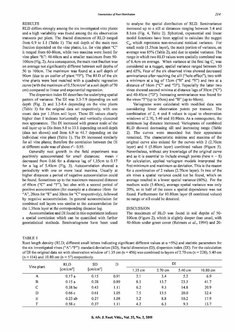
RESULTS RLD differs strongly among the six investigated vine plants and a high variability was found among the six observation transects per plant. The fractal dimension of RLD ranged from 0.9 to 1.1 (Table 1). The soil depth of the main root fraction depended on the vine plants, i.e. for vine plant "C" it ranged from 60-80cm, while two maxima were found for vine plant "E": 40-60cm and a smaller maximum from 90-100cm (Fig. 2). As a consequence, the main root fraction was on average not significantly different between soil depths of 50 to 100cm. The maximum was found at a soil depth of 90cm (due to an outlier of plant "D"). The RLD of the six vine plants were best matched with a quadratic regression curve (with the maximum of 0.55cm/cm 3 at a soil depth of 70 cm) compared to linear and exponential regression.

The dispersion index DI describes the underlying spatial pattern of variance. The DI was 3.3-7.9 depending on soil depth (Fig. 2) and 3.2-8.4 depending on the vine plants (Table 1) for the original data set respectively, with one count data per 1.35cm soil layer. These DI values clearly higher than 1 indicate horizontally and vertically clustered root appearance. The DI increased with greater scale of the soil layer up to DIs from 5.8 to 33.1 depending on soil depth (data not shown) and from 6.9 to 41.7 depending on the individual vine plant (Table 1). The DI increased similarly for all vine plants; therefore the correlation between the DI at different scale was of about r 2= 0.95.

Generally root growth in the field experiment was positively autocorrelated for small distances: mean r decreased from 0.66 for a distance lag of 1.35cm to 0.17 for a lag of 5.40cm (Fig. 3). Autocorrelation showed a periodicity with one or more local maxima. Usually at higher distances a period of negative autocorrelation could be found. Sometimes up to the maximum measured distance of 60cm ("C" and "F"), but also with a second period of positive autocorrelation (for example at a distance 10cm for "A", 20cm for "E" and 30cm for "C" respectively), followed by negative autocorrelation. In general autocorrelation for combined soil layers was similar to the autocorrelation for the 1.35cm layer at the corresponding distance lag.

Autocorrelation and DI found in this experiment indicate a spatial correlation which can be quantffied with further geostatistical methods. Semivariograms have been used

to analyse the spatial distribution of RLD. Semivariance increased up to a sill at distances ranging between 5.4 and 8.1cm (Fig. 4, Table 2). Spherical, exponential and linear model functions have been applied to calculate the nugget Co, which represents non-structural residual variance. For small scale (1.35cm layer), the main portion of variance, on average was 85% (Table 2), and due to spatial variance. The range in which two RLD values were spatially correlated was of 6.4cm on average. When variance at the first lag C 1 was considered as a nugget, spatial variance ranged between 50 and 65%. Four of the six observed vines showed decreased semivariance after reaching the sill ("hole effect"), two with a minimum at a lag of 12cm ("B" and "E") and two at a distance of 16cm ("C" and "D"). Especially the latter two vines showed second minima at distance lags of 30cm ("C") and 40-45cm ("D"). Increasing semivariance was found for the vines "F"(up to 50cm) and "B" (up to 60cm).

Variograms were calculated with modified data sets considering fewer observation points per transect. The combination of 2, 4 and 8 values is equal to observation windows of 2.70, 5.40 and 10.80cm. As a consequence, the minimum lag distance increased. Variograms of combined RLD showed decreasing sill and increasing range (Table 2). The curves were smoothed but their appearance remained. The characteristic minima and maxima of the original curve also existed for the curves with 2 (2.70cm layer) and 4 (5.80cm layer) combined values (Figure 5). Nevertheless, without any knowledge of the original curve and as it is essential to include enough points (here n = 8) for calculation, applied variogram models interpreted the first minimum and maximum as deviation. This is the reason for a combination of 2 values (2.70cm layer). In two of the six vines a spatial variance could not be found, which on average resulted in a lower spatial variance (60%). For the medium scale (5.40cm), average spatial variance was only 20%, as in half of the cases a spatial dependence was not found. Furthermore for 10.80cm layer (8 combined values) no range or sill could be detected.

DISCUSSION The maximum of RLD was found in soil depths of 50- 100cm (Figure 2), which is slightly deeper than usual, with 40-60cm under green cover (Reimers et al., 1994) and 20-

TABLE 1 Root length density (RLD; different small letters indicating signfficant different values at a =5%) and statistic parameters for the six investigated vines ("A"-"F"): standard deviation (SD), fractal dimension (D), dispersion index (DI). For the calculation of DI the original data set with observation window of 1.35 cm (n = 456) was combined to layers of 2.70 cm (n = 228), 5.40 cm (n = 114) and 10.80cm (n = 57) respectively.

Vine plant RLD 3 [cm/cm]

SD 3 [cm/cm ]

D 1.35 cm 2.70 cm

DI

5.40 cm 10.80 cm A 0.17 a 0.15 0.91 2.1 3.4 5.2 6.9 B 0.15 a 0.28 0.89 8.3 13.7 23.3 41.7 C 0.38bc 0.43 1.11 6.2 9.3 14.8 20.9 D 0.66c 0.61 1.05 7.5 13.5 20.0 32.4 E 0.23 ab 0.27 1.08 5.2 8.8 10.2 17.9 F 0.58c 0.37 1.11 4.2 6.3 9.3 13.7


215 Geostatistics ofRoot Disfribution

1.0 z A -.-- 1.35 cmLayer -0--- 2.70 cml.ayer 1.0 a B 1.35 cm[4yer -0--- 2.70 cm[4yer

01020 405060 Lag cm) Lag cm)

C - 1.35 cm[4yer -0--- 2.70 cmLayer D 1.35 cm[4yer -0--- 2.70 cm[4yer 1.0 1.0

0 10 20 g jQ() 40 50 60 0 10 20 Jg°() 40 50 60

E 1.35 cmLayer -0--- 2.70 cml2yer F -s--- 1.35 cm[4yer 1.0 1.0

-o- 2.70 cm[4yer 5.40 cmLayer A1O.8O cmLayer 5.40 cm[4yer

0.5 \ '..

0.5 A. 10.80 cm[4yer 1.:.•

S..

0 10 20L-JO(-)40 50 60 0 10 20 Jgm) 40 50 60

FIGURE 3 Autocorrelation of RLD data as a function of observation distance h with the vine plants "A"-"F". The original RLD data

(one value per 1.35cm layer) were combined to 2.70, 5.40 and 10.80cm layers respectively.

l)oA.Bc ADDE -F 2)0 A • B A C

AD 0 E • F -A -B -C -D -E -F Mean Spherical

- E 1.0 120 U

/ I A A A A

WO Sill . .

0.8 / 80

0.6 60

____ .. SPatiahariance

C0A •••• n 40

.02 p •'

DO . 020

- ____________________________ - Nugget ariance 0.0 0

0 / 10 20

0 / 10 20

Range a Lag h [cm] Range a Lag h [cm]

FIGURE 4 Experimental variograms of RLD distribution for the individual plants ("A"-"F") with the fitted model variograms (solid

lines) up to lag h=12 cm. Semivariance y (h) is given in 1) absolute values [(cm/cm 3)2] and in 2) relative values [% of C]. Model parameters range (a), sill (C = total variance), nugget variance (lag h=0: CO ; lag h=1: C) and spatial variance (C- C0)

IC are indicated for vine plant "D" in 1) and for the mean in 2)

40cm without green cover (McLean et al., 1992; Reimers et al., 1994). This discrepancy can be explained in part by interaction between soil and minirhizotron (Upchurch & Ritchie, 1983; McMichael & Taylor, 1987; Vos and

Groenwold, 1987). Root observation is mostly not done on individual plants

but on populations, so root-root interactions have to be considered. Competition among apple trees influences root



0.2 A_• 1.35 cmLayer -0--- 2.70 cmLayer 0.8 B_• 1.35 cm Layer -0--- 2.70 cmLayer

- --A- - - 5.40cmLayer - - - s-- - 10.80cmLayer - --A- - - 5.40 cmLayer - - -A- - - 10.80 cmLayer

nno C • 1.35 cmLayer -0--- 2.70 cmLayer

1.0 - - -A-- - 5.40cmLayer - -- s- - - 10.80cmLayer j

0 10 20 30 40 50 60 Lag h [cm]

0 10 20 30 40 50 60 Lagh [cm]

D • 1.35 cm Layer -0--- 2.70 cm Layer - - -A- - - 5.40 cm Layer - - -- - - 10.80 cm Layer

0 10 20 30 40 50 60 Lag h [cm]

0 10 20 30 40 50 60 Lag h [cm]

' 0.4 E • 1.35cmLayer -0--- 2.70cmLayer 0.8 - - -A- - - 5.40 cmLayer - - -A- - - 10.80 cmLayer

0

0.2 IY. fo_o 0-o0 0.4

0.0

F • 1.35 cm Layer -0--- 2.70 cm Layer

- --A- - - 5.40 cmLayer - - -A-- -10.80 cmLayer

f,r , %A- . 4 . -A% 'A.

0 10 20 30 40 50 60 Lagh [cm]

0 10 20 30 40 50 60 Lag h [cm]

FIGURE 5 The semivariance of RLD distribution for the original data set (1.35cm layer) and for combined RLD values for the vine

plants "A" to "F" (2.70, 5.40 and 10.80cm layers: two, four and eight values were combined respectively).

distribution with depth (Atkinson, 2000). In a Riesling/5C vineyard 1km from the location of this trial and under similar conditions using the monolith method, Viehauser and Adam (2005) found the highest RLD in soil depths of 70-85cm when vines were spaced 2.4 x 2.Om and at a maximum in depths of 130-145cm when planted spaced 0.6 x 2.0m. When comparing root depth, the plant density has to be considered.

The fractal dimension D differs from the concept of the other geostatistic parameters used here, because D does not describe clustering but "self-similarity". Self-similarity in this case is not concerned with the three-dimensional branching of root, but with the one-dimensional RLD curve. When calculating the fractal dimension D, the range in which box count is done is important. In this experiment, the boxes ranged from 2cm/cm 3 x 20cm to 0.3cm/cm 3 x 3cm. As a result, D ranged between 0.9 and 1.1 depending on the individual plant, which was not correlated with DI, autocorrelation and spatial variance.

The results show that vitis roots were not regularly

distributed in the soil. The dispersion index DI - one of the simplest geostatistic parameters - indicated root clustering (Fig. 2). This was confirmed by autocorrelation (Fig. 3) and semivariance (Figs 4 and 5), which specffied the type of clustering. The DI ranged from 2.1 ("A") - 8.3 ("B"). Higher values of DI indicated a more intense clustering and increased with increasing autocorrelation for small lags. In response to soil structure, the clustering of roots was also found by Tardieu and Manichon (1986), Tardieu (1988a,b,c), Logsdon and Allmaras (1991) and Vamerali et al. (2008) for maize. In the variograms, the sill indicates the maximum of variance depending on the observation distance. This sill was reached at ranges of 5.4-8.1cm for small scale (1.35cm soil layer). Where the autocorrelation was highest, the sill was reached at a greater distance. Vine plants "C" and "D" showed an autocorrelation of 0.8 at lag 1.35cm, and 0.4-0.5 at lag 4cm respectively, compared to plants "A" and "E" with an autocorrelation of about 0.5 at lag 1.35cm and an autocorrelation of 0.2 and -0.1 at lag 4cm


217

Geostatistics ofRoot Disfribution

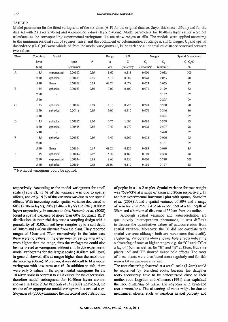
TABLE 2 Model parameters for the fitted variograms of the six vines (A-F) for the original data set (layer thickness 1.35cm) and for the data set with 2 (layer 2.70cm) and 4 combined values (layer 5.40cm). Model parameters for 10.40cm layer values were not calculated as the corresponding experimental variograms did not show ranges or sills. The models were applied according to the minimum residual sum of squares (mrss) and the coefficient of determination r 2. Range a, sill C, nugget CO and spatial dependence (C- C 0)/C were calculated from the model variograms. C 1 is the variance at the smallest distance observed between two values. Plant Combined

layer

(cm)

Model

mrss

(cm/cm3)2

r2

Range

a

cm

Sill

C

(cm/cm3)2

Nugget

C0 C1

(cm/cm3)2 (cm/cm3)2

Spatial dependence

C- C0/C

%

A 1.35 exponential 0.00002 0.99 5.60 0.113 0.000 0.052 100

2.70 spherical 0.00001 0.96 8.10 0.089 0.020 0.053 78

5.40 linear 0.00003 0.39 43.20 0.078 0.053 0.053 32

B 1.35 spherical 0.00083 0.89 7.00 0.400 0.071 0.179 82

2.70 - 0.137

5.40 - 0.205 0*

C 1.35 spherical 0.00012 0.99 8.10 0.725 0.220 0.330 70

2.70 spherical 0.00116 0.89 9.00 0.510 0.070 0.246 86

5.40 - 0.294

D 1.35 spherical 0.00017 1.00 6.75 1.090 0.080 0.369 93

2.70 spherical 0.00535 0.86 7.40 0.970 0.020 0.507 98

5.40 - 0.498

E 1.35 spherical 0.00041 0.89 5.40 0.260 0.013 0.096 95

2.70 - 0.131

5.40 linear 0.00004 0.67 43.20 0.126 0.083 0.080 35

F 1.35 spherical 0.00042 0.97 5.40 0.460 0.100 0.228 78

2.70 exponential 0.00034 0.98 8.60 0.350 0.000 0.210 100

5.40 spherical 0.00024 0.95 33.00 0.310 0.130 0.167 58

* No model variogram could be applied.

respectively. According to the model variograms for small scale (Table 2), 85 % of the variance was due to spatial effects, and only 15 % of the variance was due to non spatial effects. With increasing scale, spatial variance decreased to 60% (2.70cm layer), 20% (5.40cm layer) and 0% (10.80cm layer) respectively. In contrast to this, Vamerali et al. (2008) found a spatial variance of more than 60% for maize RLD distribution. In their trial they used a sampling design with a granularity of 10.00cm soil layer samples up to a soil depth of 100cm and a 40cm distance from the plant. They reported ranges of 57cm and 77cm respectively. In the latter case there were no values in the experimental variograms which were higher than the range, thus the variograms could also be interpreted as variograms without sill. In this experiment, model variograms for the largest scale (10.40cm soil layer) in general showed sills at ranges higher than the maximum distance lag (60cm). Moreover, it was difficult to fit a model variogram with low mrrs and r2. In addition to this, there were only S values in the experimental variograms for the 10.40cm scale in contrast to> 10 values for the other scales, therefore model varioagrams for 10.40cm layers are not shown 1 in Table 2. As Vamerali et al. (2008) mentioned, the choice of an appropriate model variogram is a critical step. Stoyan et al. (2000) examined the horizontal root distribution

of poplar in a 1 x 2 m plot. Spatial variance for root weight was 75%-93% at a range of 85cm and 20cm respectively. In another experimental horizontal plot with spruce, Scattolin et al. (2008) found a spatial variance of 50% and a range of 7cm for vital root tips in an experiment at a soil depth of 35cm and a horizontal distance of 350cm from the collar.

Although spatial variance and autocorrelation are qualitatively interdependent phenomena, it was difficult to deduce the quantitative values of autocorrelation from spatial variance. Moreover, the DI did not correlate with spatial variance although both are parameters that qualify clustering. Variograms often showed hole effects indicating a clustering of roots at higher ranges, e.g. for "C" and "D" at a lag of 16cm as well as for "B" and "E" at 12cm. But vine plants "A" and "F" showed minor hole effects. The roots of these plants were distributed more regularly and for this reason DI values were smallest. The root clustering observed at a small scale (1-2cm) could be explained by branched roots, because the daughter roots necessarily have to be concentrated close to their mother root. Logsdon and Allmaras (1991) also explained the root clustering of maize and soybean with branched root connections. The clustering of roots might be due to mechanical effects, such as variation in soil porosity and


Geostatistics of Root Disfribution

218

soil strength which influence root growth. In addition, root elongation decreases with compaction of soil or growth might be prevented if the strength of the soil is too high (Barley, 1962). As roots are deflected by obstacles in the soil and since the anysotropy of vitis roots is oriented mainly vertically, there are zones with lower RLD below obstacles. Tardieu (1988a) called this a 'shadow effect'. On the other hand, especially in compact soils, roots prefer growing in pores like cracks and earthworm channels (Tardieu 1988a). Soil pores can also be caused by inferior soil-to-minirhizotron contact.

Variation in water and nutrients in the soil are further reasons for root clustering (Robinson, 1994). Water or nutrient patches might result in clustering at small scale (1.35cm) and also at greater scale (10.40cm). In this experiment, the clustering of roots could also be found at dm scale as it was indicated by trend regression and the DI. 'Vitis root distribution followed a systematic trend with an RLD maximum at a soil depth of 70cm. Before calculating the variograms, this trend was removed from the original data due to the condition of stationarity. Therefore, variograms indicated no spatial clustering at greater scale.

CONCLUSION Various parameters of geostatistical analysis showed spatial dependence for vertical RLD distribution for vitis. For data measured at a small scale, a spatial variance of about 85% could be found at a range of Scm (1.35cm soil layer sample) and about 60% up to a range of 8cm (2.70cm soil layer sample) respectively. This autocorrelation of root distribution can be explained by soil heterogeneity and root branching. At medium scale (5-10cm) the spatial variance decreased to 0-20%. Variograms are a useful tool to improve root sampling. According to this trial, unknown points of a sample can be estimated up to a distance of 5cm. As this experiment was restricted to vertical root distribution, further investigations should evaluate variograms for horizontal RLD data.

LITERATURE CITED

Aiken, R.M., Jawson, M.D., Grahammer, K. & Polymenopoulos, A.D., 1991. Positional, spatially correlated and random components of variability in carbon dioxide efflux. J. Environ. Qual. 20, 301-308.

Atkinson, D., 2000. Root characteristics: Why and what to measure. In: Smit, A.L., Benough, AG., Engels, C., Van Noordwijk, M., Pellerin, S. & Van de Gejin, S.C., (eds). Root Methods - A Handbook. Berlin, Heidelberg, New York, 1-32.

Barnsley, M., 1988. Fractals everywhere. Academic Press, London.

Bengough, AG., Castrignano, A., Pages, L. & Van Noordwijk, L., 2000. Sampling strategies, scaling, and statistics. In: Smit, A.L., Benough, AG., Engels, C., Van Noordwijk, M., Pellerin, S. & Van de Gejin, S.C., (eds). Root Methods Handbook. Berlin, Heidelberg, New York, 147-174.

Böhm, W., 1979. Methods of Studying Root Systems. Ecological Studies 33, Springer, Berlin, Heidelberg, New York, p. 187.

Bottcher, J. & Strebel, 0., 1988. Spatial variability of groundwater solute concentrations at the water table under arable land and coniferous forest. Parti: Methods for quantif'ing spatial variability (geostatistics, time series analysis, Fourier transform smoothing). Z. Pflanzenernahr. Bodenk. 151, 185-190.

Buckland, ST., Campbell, C.D., Mackie-Dawson, L.A., Horgan, G.W. & Duff, El., 1993. A method for counting roots observed in minirhizotrons and their theoretical conversion to root length density. Plant Soil 153, 1-9.

Dahiya, IS., Anlauf, R., Kersebaum, K.C. & Richter, J., 1984. Spatial variability of some nutrient constituents of an Alfisol from loss. II. Geostatistical analysis. Z. Pflanzenernähr. Bodenk. 148, 268-277.

Dale, M.R.T., Dixon, P., Fortin, M.-J., Legrende, P., Myers, D.E. & Rosenberg, MS., 2002. Conceptual and mathematical relationships among methods for spatial analysis. Ecography 25, 55 8-577.

Dutter, R., 1985. Geostatistik. BG Teubner, Stuttgart.

Fitter, A.H., 1991. Characteristics and functions of root systems. In: Waisel, Y., Eshel, A. & Kafkafi, U., (eds) Plant Roots, the Hidden Half. Marchel Dekker Inc. New York, pp. 3-25.

Isaaks, E.H. & Srivastava, R.M., 1989. Applied Geostatistics, Oxford Univ. Press, New York.

Jackson, B.B. & Caldwell, M.M., 1993. Geostatistical patterns of soil heterogeneity around individual perennial plants. J. Ecol. 81, 683-692.

Lehnart, R., Michel, H., Lohnertz, 0. & Linsenmeier, A., 2008. Root dynamics and pattern of Riesling on SC rootstock using minirhizotron. Vitis 47, 197-200.

Linsenmeier, A., Lehnart, R., Lohnertz, 0. & Michel, H., 2010. Investigation of grapevine root distribution by in situ minirhizotron observation. Vitis 49, 1-6.

Logsdon, S.D. & Alhnaras, R.R., 1991. Maize and soybean clustering as indicated by root mapping. Plant Soil 131, 169-176.

Mandelbrot, B.B., 1983. The fractal Geometry of Nature. Freeman, New York, USA, p. 468.

McLean, M., Howell, G.S. & Smucker, A.J.M., 1992. A minirhizotron system for in situ root observation studies of seyval grapevines. Am. J. Enol. Vitic. 43, 87-89.

Manusco, 5., 1999. Fractal geometry-based image analysis of grapevine leaves using the box counting algorithm. Vitis 38, 97-100.

Matheron, G., 1965. Les variables regionalisées et leur estimation. Thesis, Masson, Paris.

McMichael, B.L., Taylor, H.M., 1987. Application and Limitations of Rhizotrons and Minirhizotrons. In: Taylor, H.M., (ed) Minirhizotron Observation Tubes: Methods and Applications for Measuring Rhizophere Dynamics, ASA Special Publication Number 50, 1-13.

Mohr, H.D., 1989. Untersuchungen zum Wachstum von Rebwurzeln in Wurzelbeobachtungskasten. Deutsches Weinbau-Jahrbuch 40, 87-96.

McMichael & Taylor, 1987.

Nielsen, K.L., Miller, C.R., Beck, D. & Lynch, J.P., 1999. Fractal geometry of root systems: Field observations of contrasting genotypes of common bean (Phaseolus vulgaris L.) grown under different phosphorus regimes. Plant Soil 206, 181-190.

Reimers, H., Steinberg, B. & Kiefer, W., 1994. Ergebnisse von Wurzeluntersuchungen an Reben bei offenem und begruntem Boden. Vitic. Enol. Sci. 49, 136-145.

Robinson, D., 1994. The responses of plants to non-uniform supplies of nutrients. New Phytol. 127, 63 5-674.

Salas, E., Ozier-Lafontaine, H. & Nygren, P., 2004. A fractal root model applied for estimating the root biomass and architecture in two tropical legume tree species. Ann. For. Sci. 61, 337-345.

S. Afr. J. EnoL Vitic., Vol. 32, No. 2,2011

219 Geostatistics ofRoot Disfribution

Scattolin, L., Boizon P. & Montecchio, L., 2008. A geostatistical model Tardieu, F., 1994. Growth and function of roots and of root systems to describe root vitality and ectomycorrhization in Norway spruce. Plant subjected to soil compaction. Towards a system with multiple signalling. Biosystems 142 (2), 391-400. Soil Tillage Res. 30, 217-243.

Smart, D.R., Schwass, E., Lasko, A. & Morano, L., 2006. Grapevine rooting patterns: A comprehensive analysis and review. Am. J. Enol. Vitic. 57, 89-104.

Smit, A.L., George, E. & Groenwold, J., 2000. Root observation and measurements at (transparent) interfaces with soil. In: Smit, A.L., Benough, A.G., Engels, C., Van Noordwijk, M., Pellerin, S. & Van de Gejin, S.C., (eds). Root Methods - A Handbook. Berlin, Heidelberg, New York, pp. 23 5-272.

Southey, J.M., 1992. Root distribution of different grapevine rootstocks on a relatively saline soil. S. Afr. J. Enol. Vitic. 13, 1-9.

Stoyan, H., De-Pollo, H., Böhm, S., Robertson, G.P. and Paul, E.A. 2000. Spatial heterogeneity of soil respiration and related properties at the plant scale. Plant Soil 222, 203-214.

Tardieu, F., 1988a. Analysis of spatial variability of maize root density. I. Effect of wheel compaction on the spatial arrangement of roots. Plant Soil 107,259-266.

Tardieu, F., 1988b. Analysis of spatial variability of maize root density. II. Distances between roots. Plant Soil 107, 267-272.

Tardieu, F., 1988c. Analysis of spatial variability of maize root density. ifi. Effect of wheel compaction on water extraction. Plant Soil 109, 257-262.

Tardieu, F. & Manichon, H., 1986. Caractérisation en tant que capteur d'eau de l'encrainement du mais en parcelle cultivée. II. Une méthode d'étude de la repartition verticale et horizontale des racines. Agronomie 6, 4 15-425.

Upchurch, D.R. & Ritchie, J.T., 1983. Root observations using a video recording system in mini-rhizotrons. Agron. 1 75, 1009-1015.

Van Noordwijk, M., Spek, L.Y. & De Willigen, P., 1994. Proximal root diameter as predictor of total root size for fractal branching models. I. Theory. Plant Soil 164, 107-117.

Vamerali, T., Guarise, M., Ganis, A., Zanetti, F. & Mosca, G., 2008. Studying root distribution with geostatistics. Plant Biosystems 142(2), 428-433.

Viehauser, Y. & Adam, A., 2005. Untersuchungen zum Wurzel- und Nahrstoflh,rofil bei unterschiedlichen Pflanzdichten bei der Rebsorte Riesling. Thesis Fachhochschule Wiesbaden, Fachbereich Geisenheim, Germany.

Vos, J., Groenwold, J., 1987. The Relation between Root Growth along Observation Tubes and in Bulk Soil. In: Taylor, H.M., (ed) Minirhizotron Observation Tubes: Methods and Applications for Measuring Rhizophere Dynamics. ASA Special Puplication Number 50, 127-156.


geostatistical analysis and scaling of grapevine root ... · geostatistical analysis and scaling of...

Documents