geoscience australia record 2006/xx · geoscience australia, record 2007/11, 133pp. correspondence...
TRANSCRIPT
G E O S C I E N C E A U S T R A L I A
S P A T I A L I N F O R M A T I O N F O R T H E N A T I O N
i
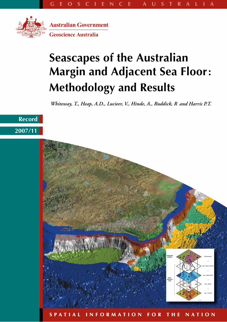
Geoscience Australia Record 2007/11
Seascapes of the Australian Margin and Adjacent Sea Floor
Methodology and Results
Tanya Whiteway1, Andrew D. Heap1, Vanessa Lucieer2, Alan Hinde*1, Ryan Ruddick1,
and Peter T. Harris1
1. Geoscience Australia, GPO Box 378, Canberra, ACT 2601 2. Tasmanian Aquaculture and Fisheries Institute, Private Bag 49, Hobart, TAS 7053
* retired.
ii
Department of Industry, Tourism & Resources Minister for Industry, Tourism & Resources: Senator The Hon. Ian Macfarlane, MP Parliamentary Secretary: The Hon. Bob Baldwin, MP Secretary: Mark Paterson
Geoscience Australia Chief Executive Officer: Dr Neil Williams © Commonwealth of Australia 2007 This work is copyright. Apart from any fair dealings for the purposes of study, research, criticism or review, as permitted under the Copyright Act 1968, no part may be reproduced by any process without written permission. Copyright is the responsibility of the Chief Executive Officer, Geoscience Australia. Requests and enquiries should be directed to the Chief Executive Officer, Geoscience Australia, GPO Box 378, Canberra City, ACT 2601, Australia. ISSN: 1448 - 2177 ISBN: 978 1 921236 38 9 (Hardcopy) ISBN: 978 1 921236 40 2 (Web) GeoCat No. 65152 Bibliographic reference: Whiteway, T., Heap, A.D., Lucieer, V., Hinde, A., Ruddick, R. & Harris, P.T. (2007). Seascapes of the Australia Margin and Adjacent Sea Floor: Methodology and Results. Geoscience Australia, Record 2007/11, 133pp. Correspondence for feedback: Sales Centre Geoscience Australia GPO Box 378 Canberra ACT 2601 [email protected] Geoscience Australia has tried to make the information in this product as accurate as possible. However, it does not guarantee that the information is totally accurate or complete. Therefore, you should not rely solely on this information when making a commercial decision.
iii
Contents Page List of Figures .......................................................................................................vi List of Tables ........................................................................................................ x Acknowledgements............................................................................................ xi Executive Summary............................................................................................xii Part 1 – Introduction........................................................................................... 13
1.1. Introduction ............................................................................................................. 13 1.2. The Seascape Approach.......................................................................................... 14 1.3. Application of Biophysical Data for Seascapes................................................... 16
Part 2 – Seascape Classifications ..................................................................... 20
2.1. Introduction ............................................................................................................. 20 2.2. Aim............................................................................................................................ 20 2.3. Methodology............................................................................................................ 20
2.3.1. Study Areas .......................................................................................................... 20 2.3.2. Input Data ............................................................................................................ 23 2.3.3. Iterations............................................................................................................... 26 2.3.4. Classification Methodology................................................................................... 29 2.3.5. Cluster Validation................................................................................................. 33 2.3.6. Classification Analysis ......................................................................................... 34
2.4. Results....................................................................................................................... 35 2.4.1. Iteration 1 – National Marine Bioregionalisation 2005 ....................................... 35 2.4.2. Iteration 2 – Application to Regional Marine Planning. ..................................... 35
2.5. Discussion................................................................................................................. 42 2.5.1. General Discussion of Results .............................................................................. 42 2.5.2. Potential Improvements........................................................................................ 44
2.6. Conclusion................................................................................................................ 45 Part 3 – Uncertainty Analysis and Methodology Verification .................. 47
3.1. Introduction ............................................................................................................. 47 3.2. Aim............................................................................................................................ 47 3.3. Methodology............................................................................................................ 47
3.3.1. Study Area ............................................................................................................ 47 3.3.2. Input Data ............................................................................................................48 3.3.3. Classification Methodology................................................................................... 49 3.3.4. Fuzzy Classification for Selected Class Numbers................................................. 50 3.3.5. Uncertainty Analysis – Confusion Maps............................................................. 50
3.4. Results....................................................................................................................... 51 3.4.1. Cluster Validity Analysis ..................................................................................... 51
iv
Page 3.4.2. Uncertainty Analysis – Confusion Maps .............................................................51 3.4.3. Final Classification Results ..................................................................................53
3.5. Discussion.................................................................................................................55 3.5.1. General Discussion of Results ..............................................................................55
3.6. Conclusion................................................................................................................59 Part 4 – Focal Variety Analyses........................................................................ 60
4.1. Introduction..............................................................................................................60 4.2. Aim ............................................................................................................................60 4.3. Methodology ............................................................................................................60
4.3.1. Study Areas...........................................................................................................60 4.3.2. Input Data.............................................................................................................60 4.3.3. Focal Variety Analysis ..........................................................................................60
4.4. Results .......................................................................................................................64 4.4.1. Focal Variety Analysis Results .............................................................................64
4.5. Discussion.................................................................................................................69 4.6. Conclusion / Recommendation .............................................................................71
Part 5 – References.............................................................................................. 72 Part 6 – Appendices............................................................................................ 76
6.1. Appendix A – Crisp Cluster Validity Measures .................................................76 6.1.1. Distance Ratio and Weighted Distance Ratio.......................................................76 6.1.2. Calinski-Harabasz Pseudo F-statistic ...................................................................77
6.2. Appendix B – Iteration 1 Results...........................................................................78 6.2.1. Initial Classifications ............................................................................................78 6.2.2. Addition of Sea Floor Temperature .......................................................................87 6.2.3. Addition of Slope, Primary Production and Effective Disturbance......................94
6.3. Appendix C – Iteration 2 Results (Northern Planning Region) ......................108 6.3.1. Northern Planning Area (Run 1, Original Boundary) ......................................108 6.3.2. Northern Planning Area (Run 2, Original Boundary) ......................................108 6.3.3. Northern Planning Area (Run 3, Original Boundary) ......................................112 6.3.4. Northern Planning Area – Reduced Variable Set (Runs 4 & 5, Original
Boundary)...........................................................................................................1156.3.5. Northern Planning Region (Run 6NPR, Revised Boundary) ............................118
6.4. Appendix D – Iteration 2 Results (South West Planning Region) ..................125 6.4.1. South West Planning Region (Run 1SWPR).....................................................125 6.4.2. South West Planning Region – Sea Floor Temperature Extrapolated
(Run 2SWPR). ...................................................................................................125 6.4.3. South West Planning Region – Revised Gravel and Mud (Run
3SWPR) .............................................................................................................128 6.5. Appendix E – Fuzzy Cluster Validity Measures...............................................132
6.5.1. Bezdek’s PC and PE Indices................................................................................132 6.5.2. Fuzzy Hyper Volume ..........................................................................................132 6.5.3. Xie-Beni (XBM) Index........................................................................................132

v
6.5.4. PBMF Index ....................................................................................................... 132 6.5.5. Partition Coefficient and Exponential Separation Index (PCAES).................... 133
vi
List of Figures Page Part 1 – Introduction .......................................................................................... 13
Figure 1.1. Schematic diagram of seascapes. ..............................................................15 Figure 1.2. Hierarchical classification of marine habitats. ........................................16 Figure 1.3. Distribution of sediment samples in MARS database. ..........................17 Figure 1.4. Photographs of North West Shelf seabed habitats. ................................19
Part 2 – Seascape Classifications ..................................................................... 20
Figure 2.1. Map of extents for areas in initial trial classifications. ...........................21 Figure 2.2. Map of marine planning regions as defined by DEW. ..........................21 Figure 2.3. Map of Northern Planning Area (Original Boundary). .........................22 Figure 2.4. Map of Northern Planning Area (Final Version)....................................23 Figure 2.5. Map of South West Planning Area. ..........................................................24 Figure 2.6. Map of different cluster boundaries. ........................................................32 Figure 2.7. Graph of distance ratio for NPR classes (Run 7NPR). ...........................37 Figure 2.8. Map of seascapes for NPR (Run 7NPR). ..................................................37 Figure 2.9. Class means for NPR (Run 7NPR). ...........................................................38 Figure 2.10. Graph of distance ratio for SWPR (Run 4SWPR – on-shelf). ................38 Figure 2.11. Map of seascapes for SWPR (Run 4SWPR – on-shelf). ..........................39 Figure 2.12. Class means for SWPR (Run 4SWPR – on-shelf). ...................................39 Figure 2.13. Class means for SWPR (Run 4SWPR – off-shelf). ...................................40 Figure 2.14. Graph of distance ratio for SWPR (Run 4SWPR – off-shelf). ................41 Figure 2.15. Map of seascapes for SWPR (Run 4SWPR – off-shelf). ..........................41 Figure 2.16. Map of environmental cluster regions for NPR......................................43
Part 3 – Uncertainty Analysis and Methodology Verification .................. 47
Figure 3.1. Map showing study area for methodology verification. .......................48 Figure 3.2. Cluster validity plot for XBm. ...................................................................52 Figure 3.3. Cluster validity plot for PCAES. ...............................................................52 Figure 3.4. Graph of distance ratio for the crisp classification method...................52 Figure 3.5. Confusion map for 4 classes using the FCM algorithm.........................54 Figure 3.6. Confusion map for 6 classes using the FCM algorithm.........................54 Figure 3.7. Plot of data frequency for confusion map of 4 classes. ..........................55 Figure 3.8. Plot of data frequency for confusion map of 6 classes. ..........................55 Figure 3.9. Maximum likelihood classification maps for 4 classes. .........................56 Figure 3.10. Maximum likelihood classification maps for 6 classes. .........................57 Figure 3.11. Final 4 class classification map using fuzzy c-means.............................58 Figure 3.12. Final 4 class classification map using crisp classification. .....................58
Part 4 – Focal Variety Analyses........................................................................ 60
Figure 4.1. Geomorphology map of the Northern Planning Region.......................61 Figure 4.2. Geomorphology map of the South West Planning Region. ..................61 Figure 4.3. Schematic diagram of focal variety analysis. ..........................................62
vii
Page Figure 4.4. Map of seascape focal variety analysis for NPR..................................... 65 Figure 4.5. Map of geomorphology focal variety analysis for NPR. ....................... 65 Figure 4.6. Map of combined seascape and geomorphology focal variety
analysis for the Northern Planning Region. ........................................ 66 Figure 4.7. Map of seascape focal variety analysis for the South West
Planning Region (off-shelf). ................................................................... 67 Figure 4.8. Map of geomorphology focal variety analysis for the South
West Planning Region (off-shelf). ......................................................... 67 Figure 4.9. Map of combined seascape and geomorphology focal variety
analysis for the South West Planning Region (off-shelf). .................. 68 Figure 4.10. Map of seascape focal variety analysis for the South West
Planning Region (on-shelf)..................................................................... 69 Figure 4.11. Map of geomorphology focal variety analysis for the South
West Planning Region (on-shelf)........................................................... 70 Figure 4.12. Map of combined seascape and geomorphology focal variety
analysis for the South West Planning Region (on-shelf).................... 70 Part 6 – Appendices ............................................................................................ 76
Figure 6.1. Graph of distance ratio for East region. ................................................... 78 Figure 6.2. Map of seascapes for East region.............................................................. 79 Figure 6.3. Class means for East region....................................................................... 80 Figure 6.4. Graph of distance ratio for South West region. ...................................... 81 Figure 6.5. Class means for South West region. ......................................................... 81 Figure 6.6. Map of seascapes for South West region. ................................................ 82 Figure 6.7. Graph of distance ratio for North West region....................................... 83 Figure 6.8. Map of seascapes for North West region................................................. 84 Figure 6.9. Class means for North West region.......................................................... 85 Figure 6.10. Graphs of distance ratio for Gulf of Carpentaria region. ...................... 86 Figure 6.11. Map of seascapes for Gulf of Carpentaria region................................... 86 Figure 6.12. Class means for Gulf of Carpentaria region............................................ 87 Figure 6.13. Graphs of distance ratio for East region (sea floor temperature
added). ...................................................................................................... 88 Figure 6.14. Class means for East region (sea floor temperature added). ................ 88 Figure 6.15. Map of seascapes for East region (sea floor temperature
added). ...................................................................................................... 89 Figure 6.16. Graphs of distance ratio for East region (wave, tide and
temperature added)................................................................................. 90 Figure 6.17. Map of seascapes for East region (wave, tide and temperature
added). ...................................................................................................... 91 Figure 6.18. Class means for East region (wave, tide and temperature
added). ...................................................................................................... 92 Figure 6.19. Graphs of distance ratio for Gulf of Carpentaria region (sea
floor temperature added). ...................................................................... 92 Figure 6.20. Map of seascapes for Gulf of Carpentaria region (sea floor
temperature added)................................................................................. 93

viii
Page Figure 6.21. Class means for Gulf of Carpentaria region (sea floor
temperature added).................................................................................94 Figure 6.22. Graphs of distance ratio for East region (effective disturbance
added)........................................................................................................95 Figure 6.23. Map of seascapes for East region (effective disturbance added)..........96 Figure 6.24. Class means for East region (effective disturbance added)...................97 Figure 6.25. Graphs of distance ratio for South West region (effective
disturbance added)..................................................................................97 Figure 6.26. Map of seascapes for South West region (effective disturbance
added)........................................................................................................98 Figure 6.27. Class means for South West region (effective disturbance
added)........................................................................................................99 Figure 6.28. Graphs of distance ratio for North West region (effective
disturbance added)................................................................................100 Figure 6.29. Map of seascapes for North West region (effective disturbance
added)......................................................................................................100 Figure 6.30. Class means for North West region (effective disturbance
added)......................................................................................................101 Figure 6.31. Graphs of distance ratio for Gulf of Carpentaria region
(effective disturbance added)...............................................................101 Figure 6.32. Map of seascapes for Gulf of Carpentaria region (effective
disturbance added)................................................................................102 Figure 6.33. Class means for Gulf of Carpentaria region (effective
disturbance added)................................................................................103 Figure 6.34. Graphs of distance ratio for East and North West regions
(reduced variable set). ...........................................................................103 Figure 6.35. Map of seascapes for the East and North West regions
(reduced variable set). ...........................................................................104 Figure 6.36. Class means for the East and North West regions (reduced
variable set).............................................................................................110 Figure 6.37. Graphs of distance ratio for South West region (reduced
variable set).............................................................................................105 Figure 6.38. Map of seascapes for the South West region (reduced variable
set). ...........................................................................................................106 Figure 6.39. Class means for the South West region (reduced variable set)...........107 Figure 6.40. Graphs of distance ratio for Run 1 – Northern Planning
Region......................................................................................................109 Figure 6.41. Map of seascapes for Run 1 – Northern Planning Area.......................109 Figure 6.42. Class means for Run 1 – Northern Planning Area. ..............................110 Figure 6.43. Graphs of distance ratio for Run 2 – Northern Planning Area
(reduced variable set, effective disturbance added). ........................110 Figure 6.44. Map of seascapes for Run 2 – Northern Planning Area
(reduced variable set, effective disturbance added). ........................111 Figure 6.45. Class means for Run 2 – Northern Planning Area (reduced
variable set, effective disturbance added)..........................................111
ix
Page Figure 6.46. Graph of eigenvalues for correlation matrix for the Northern
Planning Area. ....................................................................................... 114 Figure 6.47. Graphs of distance ratio for Northern Planning Area (principal
component analysis). ............................................................................ 115 Figure 6.48. Class means for Northern Planning Area using the first six
principal components. .......................................................................... 116 Figure 6.49. Graph of distance ratio for the Northern Planning Area using 3
factors (principal component analysis). ............................................. 116 Figure 6.50. Map of seascapes for Run 3 – Northern Planning Area
(principal component analysis). .......................................................... 117 Figure 6.51. Class means for Run 3 – Northern Planning Area using the
first three principal components. ........................................................ 117 Figure 6.52. Graph of distance ratio for Run 4 – Northern Planning Area
(reduced variable set)............................................................................ 118 Figure 6.53. Map of seascapes for Run 4 – Northern Planning Area
(reduced variable set)............................................................................ 119 Figure 6.54. Class means for Run 4 – Northern Planning Area (reduced
variable set). ........................................................................................... 120 Figure 6.55. Graphs of distance ratio for Run 5 – Northern Planning Area
(smoothed log slope, reduced variable set). ...................................... 120 Figure 6.56. Map of seascapes for Run 5 – Northern Planning Area
(smoothed log slope, reduced variable set). ...................................... 121 Figure 6.57. Map of seascapes for Run 5 – Northern Planning Area
(smoothed log slope, reduced variable set). ...................................... 122 Figure 6.58. Graph of distance ratio for Run 6 – Northern Planning Region
(new boundary). .................................................................................... 122 Figure 6.59. Map of seascapes for Run 6 – Northern Planning Region (new
boundary). .............................................................................................. 123 Figure 6.60. Class means for Run 6 – Northern Planning Region (new
boundary). .............................................................................................. 124 Figure 6.61. Graph of distance ratio for the SWPR (Run 2SWPR)........................... 126 Figure 6.62. Map of seascapes for the SWPR (Run 2SWPR)..................................... 126 Figure 6.63. Class means for SWPR (Run 2SWPR) .................................................... 127 Figure 6.64. Map of available sea floor temperature data for SWPR. ..................... 127 Figure 6.65. Graphs of distance ratio for SWPR (sea floor temperature
extrapolated). ......................................................................................... 128 Figure 6.66. Map of seascapes for SWPR (sea floor temperature
extrapolated............................................................................................ 128 Figure 6.67. Class means for SWPR (sea floor temperature extrapolated)............. 129 Figure 6.68. Graph of distance ratio for SWPR (mud & gravel included).............. 129 Figure 6.69. Map of seascapes for SWPR (mud & gravel included)........................ 130 Figure 6.70. Class means for SWPR (mud & gravel included)................................. 130

x
List of Tables Page Part 1 – Introduction .......................................................................................... 13
Table 1.1. Physical seabed properties shown to correlate with benthic biota. ..........................................................................................................14
Part 2 – Seascape Classifications ..................................................................... 20
Table 2.1. List of classifications undertaken in iteration 1. .....................................27 Table 2.2. List of classifications undertaken in iteration 2. .....................................30
Part 3 – Uncertainty Analysis and Methodology Verification .................. 47
Table 3.1. Comparison of the number of classes preferred by each validity measure. .....................................................................................51
Table 3.2. Statistics of confusion maps for 4 and 6 classes. .....................................53 Part 4 – Focal Variety Analyses........................................................................ 60
Table 4.1. Parameters used in the focal variety analysis for the Northern and South West Planning Regions. .......................................................62
Part 6 – Appendices............................................................................................ 76
Table 6.1. Run 3 – Principal components for the 14 variables used for the Northern Planning Area (principal component analysis). ..............113
Table 6.2. Run 3 – Eigenvalues of the correlation matrix for the Northern Planning Area (principal component analysis). ................................114
xi
Acknowledgements This record is published with permission of the Chief Executive Officer, Geoscience Australia.
xii
Executive Summary Geoscience Australia has undertaken a classification of biophysical datasets to create seabed habitat maps (termed ‘seascapes’) for the Australian margin and adjacent sea floor. Seascapes describe a layer of ecologically meaningful biophysical properties that spatially represents potential seabed habitats. Each seascape area corresponds to a region of the seabed that contains similar biophysical properties and, by association, potential habitats and communities. The procedure adopted is inspired by the shelf classification applied in eastern Canada where physical properties (sediment type, physiography, bed roughness, wave and current regime) were used to define ecologically meaningful habitats on the Scotian Shelf. Creating seascapes as proxies for benthic marine biological communities using biophysical data is required because it is impossible to count and map the distribution of every organism in the ocean.
This report describes the iterative methods used to create the seascapes, including a detailed appendix documenting the different datasets used in each planning zone. Creating the seascapes is necessarily an iterative process whereby the available datasets are integrated in different combinations, or added as they become available, using the ERMapper™ unsupervised, crisp ISOclass classification program. In each classification only biophysical properties that have consistent and definable relationships with the benthic biota and are known in sufficient detail across Australia’s entire marine region are used to create the seascapes. An initial validation of the classification technique has been undertaken on a subset of the data for the shelf surrounding Tasmania using an alternative unsupervised fuzzy classification. Results of this validation indicate that the unsupervised classification methodology provides consistent and reliable classes for defining the seascapes.
Finally, a quantitative method designed to determine where the greatest seabed heterogeneity occurs to assist with the selection of potential sites for Marine Protected Areas was trialled on the final seascapes. This Focal Variety method conducted in ArcGIS simply counts up the number of seascape types within a specified radius (in this case 20 km). Focal variety analyses were conducted separately on the seascapes (which comprise continuous spatial data) and geomorphology (which comprise categorical spatial data) and the results combined. Areas where many different seascapes occur are considered as potential habitat diversity hotspots.
The mandate for creating the seascapes comes directly from the United Nations Convention on Biological Diversity (CBD), which Australia ratified in 1994. The CBD requires Australia to set up a system of marine protected areas for the conservation and sustainable use of threatened species, habitats and living marine resources and ecological processes. We believe that the seascapes provide a useful method for assisting in the development of this system of MPA’s by spatially representing seabed heterogeneity in a consistent, objective and robust way.
The future of seascapes and surrogacy research is to work collaboratively with marine biologists and ecologists in the formation of seascapes for marine biodiversity prediction, including undertaking targeted marine surveys to collect further physical and biological data and building combined databases that permit direct correlation of data. This research will improve the accuracy and precision with which we can predict Australia’s marine biodiversity and thus strengthen confidence in decisions about the conservation and sustainable use of Australia’s marine resources.
13
PART 1 – Introduction The purpose of this report is to detail the methods undertaken to create seascapes for the Australian margin and adjacent sea floor. The report contains sections that detail and discuss the verification and uncertainty techniques applied to create the seascapes, and to further interpret the outputs for marine management purposes. This report does not include previous work undertaken investigating the links between physical properties and the biota, upon which the seascapes are based. Further information on this concept of biophysical surrogacy is detailed in many other references (e.g., Thouzeau et al., 1991; Kostylev et al., 2001; Pitcher et al., 2002; Post et al., 2006).
1.1. INTRODUCTION Australia’s Environment Protection and Biodiversity Conservation Act, 1999 provides direction for marine management in Australian waters, including “the conservation of biodiversity by providing strong protection for threatened species and ecological communities, migratory, marine and other protected species” (Department of the Environment and Heritage (DEH), 2005; now the Department of the Environment and Water Resources (DEW). A key component of the policy is the creation of Regional Marine Plans (RMP) and a national system of representative Marine Protected Areas (NSRMPA) to help conserve marine biodiversity. The Australian government is presently preparing RMP’s and designing marine protected areas (MPA) for the area of ocean between the Australian coastline and outer boundary of the Australian Exclusive Economic Zone (AEEZ), an area of >8.4 million km2 (DEH, 2005).
Mapping benthic biota and habitats is one approach providing marine managers with information to support the RMP and MPA design process. On a smaller scale (i.e., bays and estuaries) in coastal waters an approach using seabed sampling, side-scan imagery, underwater video, and transect analysis are viable techniques, providing managers with high-resolution information to manage the whole range of biota. However, it is impossible to observe all of Australia’s marine biodiversity with current technologies and impractical to count every organism, with much of the deep-sea inaccessible to comprehensive biological sampling. To make informed decisions about the conservation and sustainable use of Australia’s marine resources would require high-quality biological data across the nation’s entire marine region, but such data do not exist. To make decisions now, managers must use what is available.
An alternative approach pioneered the United States (Greene et al., 1995) and later applied in countries including Canada (Roff & Taylor, 2000) and Ireland (Golding at al., 2004) is the classification of biophysical parameters to create broad-scale benthic habitat maps (seascapes) that can be used as a substitute for habitat type and biotic variability. Many important ecological constraints are geophysical in nature; water temperature, sediment type, depth, and bottom disturbance are major factors influencing the type and abundance of marine organisms (Golding et al., 2004). The seascape map (akin to a landscape map for underwater landscapes) can be applied as a surrogate to identify where potential benthic marine habitats may occur.
Biophysical datasets can be analysed using Geographic Information Systems (GIS) with statistical methods, to integrate spatial (quantitative) data and determine relationships between the data layers. The final integrated data layer (or seascape) is a map of potential
Seascapes of the Australian Margin
14
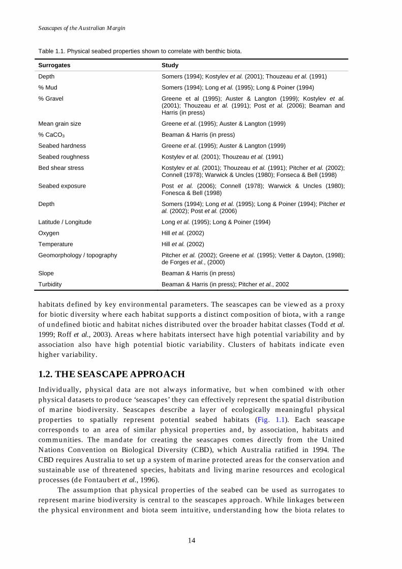
Table 1.1. Physical seabed properties shown to correlate with benthic biota.
Surrogates Study
Depth Somers (1994); Kostylev et al. (2001); Thouzeau et al. (1991)
% Mud Somers (1994); Long et al. (1995); Long & Poiner (1994)
% Gravel Greene et al (1995); Auster & Langton (1999); Kostylev et al. (2001); Thouzeau et al. (1991); Post et al. (2006); Beaman and Harris (in press)
Mean grain size Greene et al. (1995); Auster & Langton (1999)
% CaCO3 Beaman & Harris (in press)
Seabed hardness Greene et al. (1995); Auster & Langton (1999)
Seabed roughness Kostylev et al. (2001); Thouzeau et al. (1991)
Bed shear stress Kostylev et al. (2001); Thouzeau et al. (1991); Pitcher et al. (2002); Connell (1978); Warwick & Uncles (1980); Fonseca & Bell (1998)
Seabed exposure Post et al. (2006); Connell (1978); Warwick & Uncles (1980); Fonesca & Bell (1998)
Depth Somers (1994); Long et al. (1995); Long & Poiner (1994); Pitcher et al. (2002); Post et al. (2006)
Latitude / Longitude Long et al. (1995); Long & Poiner (1994)
Oxygen Hill et al. (2002)
Temperature Hill et al. (2002)
Geomorphology / topography Pitcher et al. (2002); Greene et al. (1995); Vetter & Dayton, (1998); de Forges et al., (2000)
Slope Beaman & Harris (in press)
Turbidity Beaman & Harris (in press); Pitcher et al., 2002
habitats defined by key environmental parameters. The seascapes can be viewed as a proxy for biotic diversity where each habitat supports a distinct composition of biota, with a range of undefined biotic and habitat niches distributed over the broader habitat classes (Todd et al. 1999; Roff et al., 2003). Areas where habitats intersect have high potential variability and by association also have high potential biotic variability. Clusters of habitats indicate even higher variability.
1.2. THE SEASCAPE APPROACH Individually, physical data are not always informative, but when combined with other physical datasets to produce ‘seascapes’ they can effectively represent the spatial distribution of marine biodiversity. Seascapes describe a layer of ecologically meaningful physical properties to spatially represent potential seabed habitats (Fig. 1.1). Each seascape corresponds to an area of similar physical properties and, by association, habitats and communities. The mandate for creating the seascapes comes directly from the United Nations Convention on Biological Diversity (CBD), which Australia ratified in 1994. The CBD requires Australia to set up a system of marine protected areas for the conservation and sustainable use of threatened species, habitats and living marine resources and ecological processes (de Fontaubert et al., 1996).
The assumption that physical properties of the seabed can be used as surrogates to represent marine biodiversity is central to the seascapes approach. While linkages between the physical environment and biota seem intuitive, understanding how the biota relates to

Introduction
15
Figure 1.1. Schematic diagram showing derivation of seascapes from multiple spatial layers of physical data. The seascapes represent the integrated product of the individual physical data.
physical properties is only half the story. It is equally essential to identify which physical properties are relevant. Those physical properties that show the strongest relationship with the biota (as defined by some measure of goodness of fit) are considered to be the most relevant as surrogates for biodiversity.
Relationships between physical properties and biota have been shown to exist in many studies of the marine environment (e.g., Thouzeau et al., 1991; Snelgrove & Butman, 1994; Bax & Williams, 2001; Ramey & Snelgrove, 2003). These studies show that, broadly, seabed biota have measurable and consistent relationships with many easily measured physical seabed properties (Table 1.1). A Geoscience Australia study of associations between sediment properties and benthic biota in the southern Gulf of Carpentaria (Post et al., 2006) shows that spatial changes in seabed biota are strongly related to mud and gravel content, seabed disturbance from waves and currents, water depth, and geomorphology. Specific details regarding the “surrogacy” relationships between physical variables and the biota are not treated here. More details can be found in Post et al. (2006) and the studies cited above.
While surrogates provide important clues as to how the biota are related to physical properties and which physical properties are most relevant, those studies are at a spatial scale that is generally too small to help managers make informed decisions about the conservation and sustainable use of Australia’s entire marine region. We must take the results of these studies and extrapolate them over larger distances by creating seascapes.
Geoscience Australia in conjunction with the DEW and CSIRO have prepared baseline biophysical datasets and are currently undertaking analyses of data to identify areas of highest potential habitat heterogeneity through the creation of seascapes. The information and datasets created as part of this program will be supplied to DEW. DEW, in
Seascapes of the Australian Margin
16
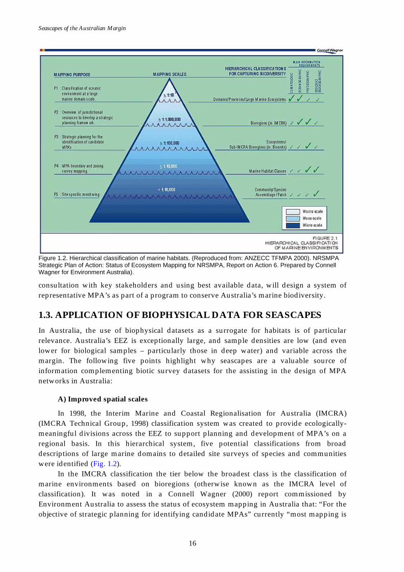
Figure 1.2. Hierarchical classification of marine habitats. (Reproduced from: ANZECC TFMPA 2000). NRSMPA Strategic Plan of Action: Status of Ecosystem Mapping for NRSMPA, Report on Action 6. Prepared by Connell Wagner for Environment Australia).
consultation with key stakeholders and using best available data, will design a system of representative MPA’s as part of a program to conserve Australia’s marine biodiversity.
1.3. APPLICATION OF BIOPHYSICAL DATA FOR SEASCAPES In Australia, the use of biophysical datasets as a surrogate for habitats is of particular relevance. Australia’s EEZ is exceptionally large, and sample densities are low (and even lower for biological samples – particularly those in deep water) and variable across the margin. The following five points highlight why seascapes are a valuable source of information complementing biotic survey datasets for the assisting in the design of MPA networks in Australia:
A) Improved spatial scales
In 1998, the Interim Marine and Coastal Regionalisation for Australia (IMCRA) (IMCRA Technical Group, 1998) classification system was created to provide ecologically-meaningful divisions across the EEZ to support planning and development of MPA’s on a regional basis. In this hierarchical system, five potential classifications from broad descriptions of large marine domains to detailed site surveys of species and communities were identified (Fig. 1.2).
In the IMCRA classification the tier below the broadest class is the classification of marine environments based on bioregions (otherwise known as the IMCRA level of classification). It was noted in a Connell Wagner (2000) report commissioned by Environment Australia to assess the status of ecosystem mapping in Australia that: “For the objective of strategic planning for identifying candidate MPAs” currently “most mapping is
Introduction
17
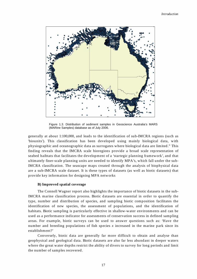
Figure 1.3. Distribution of sediment samples in Geoscience Australia’s MARS (MARine Samples) database as of July 2006.
generally at about 1:100,000, and leads to the identification of sub-IMCRA regions (such as 'biounits'). This classification has been developed using mainly biological data, with physiographic and oceanographic data as surrogates where biological data are limited.” This finding reveals that the IMCRA scale bioregions provide a broad scale representation of seabed haibtats that facilitates the development of a ‘startegic planning framework’, and that ultimately finer-scale planning units are needed to identify MPA’s, which fall under the sub- IMCRA classification. The seascape maps created through the analysis of biophysical data are a sub-IMCRA scale dataset. It is these types of datasets (as well as biotic datasets) that provide key information for designing MPA networks
B) Improved spatial coverage
The Connell Wagner report also highlights the importance of biotic datasets in the sub-IMCRA marine classification process. Biotic datasets are essential in order to quantify the type, number and distribution of species, and sampling biotic composition facilitates the identification of new species, the assessment of populations, and the identification of habitats. Biotic sampling is particularly effective in shallow-water environments and can be used as a performance indicator for assessments of conservation success in defined sampling areas. For example, biotic surveys can be used to answer questions such as: ‘Have the number and breeding populations of fish species x increased in the marine park since its establishment?’
Conversely, biotic data are generally far more difficult to obtain and analyse than geophysical and geological data. Biotic datasets are also far less abundant in deeper waters where the great water depths restrict the ability of divers to survey for long periods and limit the number of samples recovered.
Seascapes of the Australian Margin
18
Geophysical and geological data cover a much wider area, and samples can be collected in far greater concentrations than biotic samples from all water depths and seabed types (Fig. 1.3). The wide distribution of physical samples lends itself to interpolation where the data voids between sample points are filled with data based on their relationship with actual data points. In this way geophysical datasets are mapped at large scales and can cover the entire area of the AEEZ.
The relatively large distribution of geophysical and geological data means that analyses can be undertaken for the majority of the AEEZ, providing information on potential habitats for the whole region. Undertaking biotic sampling for the entire area of the AEEZ would potentially take hundreds of years. A combination of seascape mapping and biotic sampling provides datasets that can be used for rapid, initial identification of potential MPA sites in timeframes required to support the design of a national representative system of MPA’s and environmental assessments.
C) Habitat stability/disturbance (temporal scaling)
Another factor complicating the use of biotic surveys to create a complete representation of the AEEZ is that the data captured only represents a snapshot in time. As such, biotic surveys provide data about the current biodiversity but do not incorporate temporal variability. Disturbance events such as seabed slumping, river floods and cyclones have the potential to change the composition of the seabed and water properties, and can influence community and species composition and distribution, and the ability of new species to colonise a location. Even local scale disturbances such as those resulting from varying current velocity (e.g., tides) and wave power (e.g., storms) can have a profound effect on habitat and community type.
It is possible to estimate size and distribution of potential disturbances using geophysical and geological properties. For instance slope can be used to identify the location of potential slumping events, and to show the location and size of previous slumping events. In combination with records quantifying monitored disturbance events and their potential impacts on the seabed composition, potential habitat changes can be mapped through time at a larger event scale.
D) Habitats are an integral part of biodiversity
Biodiversity comprises three components: habitats (communities), species and genetics (e.g., Day & Roff, 2000), but is frequently referred to in terms of species. Without habitats species can not survive, and hence their genetic diversity will not be preserved. It is therefore just as important to recognise and protect habitats (Bax & Williams, 2001). If habitats are protected, the associated species and their genetic diversity are also protected. This is particularly important in order to conserve the potentially thousands of species that have not been scientifically described or that have yet to be discovered. Protecting a range of habitats protects a range of biodiversity. Seascape mapping is a rapid way of defining potential seabed habitats for the whole AEEZ. Using the seascapes to guide the development of MPA’s can assist in conserving a representative suite of species and their genetic variability.
E) Capturing human disturbance
One major difference between the singular application of biotic samples instead of a combined biotic and seascapes approach is the way in which anthropogenic impacts are
Introduction
19
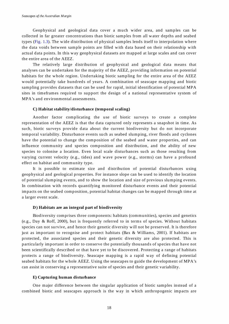
Figure 1.4. Photographs of the North West Shelf of Australia where trawling has not been undertaken (left) and where trawling has been undertaken (right). Source: Dr Keith Sainsbury, CSIRO.
treated. Seascapes maps are created based on biophysical properties, which (apart from natural disturbance regimes) do not change greatly. Therefore seascapes show potential habitats and are not biased by human impacts. In contrast, biological surveys provide information of the current (possibly disturbed) benthos. Areas that have been subject to bottom trawling can be completely stripped of any surface biota (Fig. 1.4). Moreover, humans have had a large influence on the composition and abundance marine biota. Biological surveys sample what is there, not what could be there.
Seascape mapping using geophysical and geological datasets allows for the prediction of habitat extent unbiased by the influence of human impacts. The seascape map allows inferences to be made about what biota could (or should) potentially be there. Therefore conservation measures that include protection of a percentage of all seascape habitats will include some areas of high human impact. These areas can allow for potential rehabilitation of marine biota.
20
PART 2 – Seascape Classifications
2.1. INTRODUCTION A combination of biophysical factors creates a habitat; a specialised set of conditions that influence the type and abundance of species that can live in a specific geographic province. Known relationships between biophysical properties and species can be used to map habitat and potential species distributions in the terrestrial domain, but remain largely unexplored in marine environments.
This use of biophysical datasets to map potential benthic habitats has particular appeal in Australian waters for the reasons outlined in Part 1. In the analysis presented here, biophysical data describing the seafloor morphology, substrate type and environmental parameters (water temperature and depth) are combined in a single classification whereby the input datasets are broken down into logical classes distinguished by their statistical differences. These classes likely represent different benthic (seabed) marine habitats and therefore provide a first approximation of seabed biodiversity. The following section describes methods and results for a multivariate, unsupervised classification of input datasets to create a marine habitat (or seascape) map.
2.2. AIM The aim of this work is to develop a methodology for the objective classification of marine geophysical datasets to create potential habitat maps (seascapes).
2.3. METHODOLOGY Seascapes are carried out for a number of geographic regions of offshore Australia. The methodology utilises ERMapper's ISOCLASS unsupervised classification and statistical analysis to create a number of seascape classes from input data sets available for the regions.
2.3.1. Study Areas The first step in the classification process was to determine the individual areas to be classified. An overall classification for all of Australia was excluded because some key datasets do not have complete coverage of the Australian Exclusive Economic Zone (AEEZ). Choosing smaller regions allows optimal use of the available data, and has the advantage of dividing the problem into manageable subsets.
2.3.1.1. Initial Trail Classification Areas Four areas were initially created to make maximum use of the available data. The
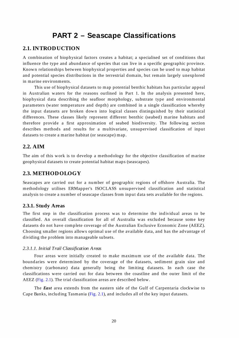
boundaries were determined by the coverage of the datasets, sediment grain size and chemistry (carbonate) data generally being the limiting datasets. In each case the classifications were carried out for data between the coastline and the outer limit of the AEEZ (Fig. 2.1). The trial classification areas are described below.
The East area extends from the eastern side of the Gulf of Carpentaria clockwise to Cape Banks, including Tasmania (Fig. 2.1), and includes all of the key input datasets.
Classification
21
Figure 2.1. Map showing the extent of areas classified in initial trial classifications.
Figure 2.2. Marine planning regions as defined by DEW, and as used for seascape classifications.

Seascapes of the Australian Margin
22
Figure 2.3. Northern Planning Area (original) boundary as originally defined by DEW, later modified.
The South West area extends along the south Australian margin from Cape Banks clockwise to Perth (Fig. 2.1), and includes no sediment data.
The North West area extends along the north west Australian margin from Exmouth clockwise to the Wessell Islands (Fig. 2.1), and includes all of the key input datasets.
The Gulf of Carpentaria area encompasses the Gulf of Carpentaria (Fig. 2.1), and does not contain carbonate data.
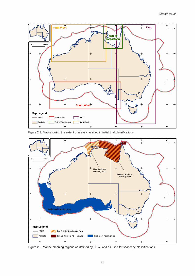
2.3.1.1. Final Classification Regions Seascapes were later created for selected planning areas (the North and South West
Planning Regions) as defined by the DEW, for MPA planning purposes. The MPA regions used in classification trials are described below.
The Original Northern Planning Area (NPA) includes the Gulf of Carpentaria and Torres Strait and extends west to the Golburn Islands in the Arafura Sea (Figs. 2.2 & 2.3). In the north it is bounded by the outer limit of the AEEZ, and to the south by the Australian coastline. It covers an area of approximately 572,000 km2 (Passlow et al., 2005).
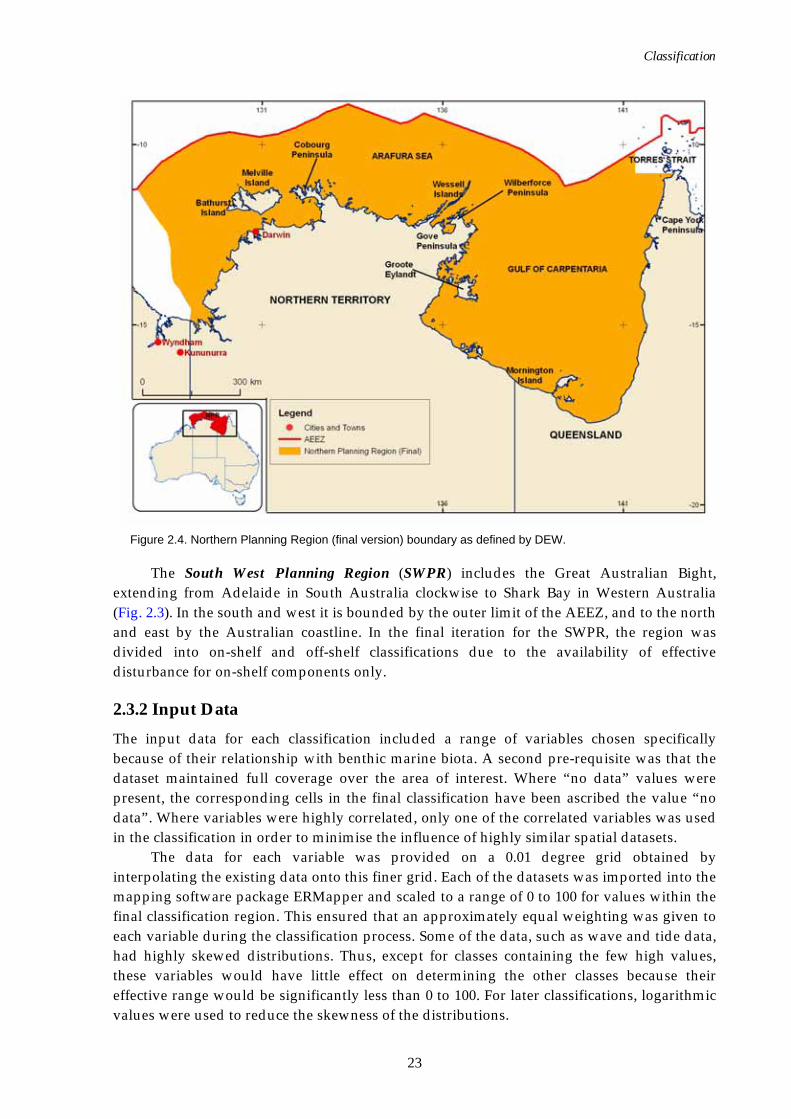
The Northern Planning Region (Final) boundary was re-defined by DEW in May 2006, and henceforth the modified area is referred to as the Northern Planning Region (NPR). The new region includes the Gulf of Carpentaria and extends west to the Northern Territory and Western Australia border (Fig. 2.4). Torres Strait is excluded. In the north it is bounded by the outer limit of the AEEZ, and to the south by the Australian coastline. It covers an area of approximately 718,590 km2 (Passlow et al., 2005).
Classification
23
Figure 2.4. Northern Planning Region (final version) boundary as defined by DEW.
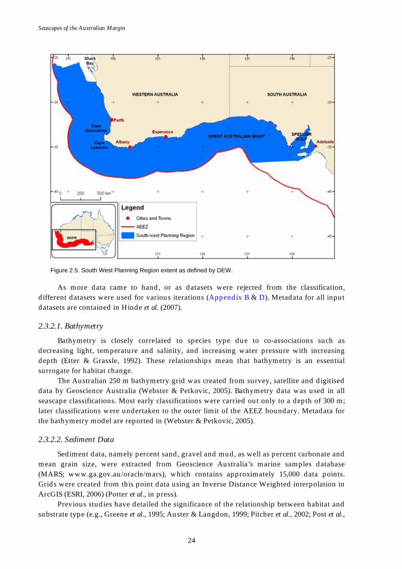
The South West Planning Region (SWPR) includes the Great Australian Bight, extending from Adelaide in South Australia clockwise to Shark Bay in Western Australia (Fig. 2.3). In the south and west it is bounded by the outer limit of the AEEZ, and to the north and east by the Australian coastline. In the final iteration for the SWPR, the region was divided into on-shelf and off-shelf classifications due to the availability of effective disturbance for on-shelf components only.
2.3.2 Input Data The input data for each classification included a range of variables chosen specifically because of their relationship with benthic marine biota. A second pre-requisite was that the dataset maintained full coverage over the area of interest. Where “no data” values were present, the corresponding cells in the final classification have been ascribed the value “no data”. Where variables were highly correlated, only one of the correlated variables was used in the classification in order to minimise the influence of highly similar spatial datasets.
The data for each variable was provided on a 0.01 degree grid obtained by interpolating the existing data onto this finer grid. Each of the datasets was imported into the mapping software package ERMapper and scaled to a range of 0 to 100 for values within the final classification region. This ensured that an approximately equal weighting was given to each variable during the classification process. Some of the data, such as wave and tide data, had highly skewed distributions. Thus, except for classes containing the few high values, these variables would have little effect on determining the other classes because their effective range would be significantly less than 0 to 100. For later classifications, logarithmic values were used to reduce the skewness of the distributions.
Seascapes of the Australian Margin
24
Figure 2.5. South West Planning Region extent as defined by DEW.
As more data came to hand, or as datasets were rejected from the classification, different datasets were used for various iterations (Appendix B & D). Metadata for all input datasets are contained in Hinde et al. (2007).
2.3.2.1. Bathymetry
Bathymetry is closely correlated to species type due to co-associations such as decreasing light, temperature and salinity, and increasing water pressure with increasing depth (Etter & Grassle, 1992). These relationships mean that bathymetry is an essential surrogate for habitat change.
The Australian 250 m bathymetry grid was created from survey, satellite and digitised data by Geoscience Australia (Webster & Petkovic, 2005). Bathymetry data was used in all seascape classifications. Most early classifications were carried out only to a depth of 300 m; later classifications were undertaken to the outer limit of the AEEZ boundary. Metadata for the bathymetry model are reported in (Webster & Petkovic, 2005).
2.3.2.2. Sediment Data
Sediment data, namely percent sand, gravel and mud, as well as percent carbonate and mean grain size, were extracted from Geoscience Australia’s marine samples database (MARS; www.ga.gov.au/oracle/mars), which contains approximately 15,000 data points. Grids were created from this point data using an Inverse Distance Weighted interpolation in ArcGIS (ESRI, 2006) (Potter et al., in press).
Previous studies have detailed the significance of the relationship between habitat and substrate type (e.g., Greene et al., 1995; Auster & Langdon, 1999; Pitcher et al., 2002; Post et al.,
Classification
25
2006). These show that the substrate type influences the location of benthic organisms. Geoscience Australia’s sediment data provides key information on the various sediment substrates in the marine environments. Further work is currently being undertaken to map the substrate for the whole of the AEEZ into hard (rock) and soft (sediment) types.
Initially all sediment data variables were included in the classification, however, sand, gravel and mud must add up to 100%. Consequently, only gravel and mud were used for later classifications, and sand became implicit in the output classification graphs. Carbonate was used in numerous iterations, but was dropped from Northern Planning Area, Gulf of Carpentaria and South West iterations because it did not have full coverage. It was finally included in the South West Planning Area iteration after further sample data were collected.
2.3.2.3. Geomorphology
The geomorphology of Australia’s continental margin was created by Geoscience Australia using techniques outlined in Harris et al. (2003). Metadata for geomorphology is contained in a DEW report (DEH, 2005). Geomorphology is considered to be broadly linked to habitats and communities. For instance, both seamounts and submarine canyons are recognised as high diversity areas, whereas the diversity across the shelf is relatively less varied.
The geomorphology dataset was used in the early classifications, although, the results were influenced by that fact that geomorphology is not a continuous variable and consisted of 21 pre-defined classes. In later classifications this dataset was used to identify further habitat variability once the seascape classification had been completed (see PART 4).
2.3.2.4. Sea Floor Temperature
Sea floor temperature (DEH, 2005) became available, and was added to the classification variables after the initial classifications had been completed. Sea floor temperature is correlated with bathymetry and hence may not add much to the classifications. However, this variable was used in all later classifications due to the fact that sea floor temperature varies with latitude (xo / degree of latitude) as well as depth, and this variation was considered important in distinguishing seascapes from the warmer northern provinces of each classification, versus those seascapes in the cooler southern provinces.
2.3.2.5. Effective Disturbance
Wave and tide excedence (percentage of time the near-bed wave and tide currents exceed bed load transport thresholds for the mean grain size), and mean wave energy, maximum tide speed were initially used as an indication of seabed exposure to energy regimes. For later classifications, these variables were replaced by effective disturbance, a single variable representing currents associated with waves, tides and low-frequency ocean currents (e.g., ocean circulation) (Hemer, 2006).
2.3.2.6. Slope
For later classifications, the slope dataset was added. The slope was initially created in ArcGIS, but was found to be inaccurate due to stepping within the input dataset in flat areas due to the cell size. This caused lines of high slope along the change in depth followed by flat areas where there was no apparent change in depth. The final slope dataset used in the
Seascapes of the Australian Margin
26
classification process was created from the bathymetry grid using ERMapper’s slope (degrees) algorithm. This algorithm applies an averaging function, thus removing the stepping artefact.
2.3.2.7. Primary Production
The primary productivity dataset created by CSIRO in 2004 using analysed satellite imagery was used in later analyses as an indication of areas where high levels of available nutrients occur. In some cases (particularly in the Northern Planning Region) this dataset picked up turbid waters as high productivity areas where they possibly were not highly productive. Although an artefact, this pattern captures differences in the coastal zone due to high turbidity.
2.3.3. Iterations Two classification iterations were undertaken using the unsupervised ISOclass classification methodology. In iteration 1 the classifications were undertaken for areas as defined by the National Marine Bioregionalisation of Australia. In iteration 2 the classifications were undertaken on Marine Planning Areas as defined by DEW.
2.3.3.1. Iteration 1 The first seascape classifications were produced in 2004 for the National Marine
Bioregionalisation of Australia (DEH, 2005). Some input datasets did not cover all coastal waters due to irregular distributions of input point sample data. As a result there is variation in the datasets used for each region as summarised in Table 2.1. In each area numerous runs were undertaken with various combinations of available input datasets in order to establish a suitable combination of input variables (refer to Table 2.1 for input datasets, and Appendix B for results). The first iterations (Run 1) were run using all available data, which included:
• bathymetry, • % carbonate, • % gravel, • % mud, • wave excedence, • tide excedence, • mean grain size, • geomorphology, • mean wave energy, and • maximum tide speed.
Later in the analysis a sea floor temperature dataset was developed and included in future classifications (Run 2). Finally, datasets for slope, primary production and effective disturbance were also produced, and were subsequently added to further classifications (Run 3). These datasets were transformed using a logarithmic transformation due to the high level of skewness in their distributions.
Classification
27
Table 2.1. List of classifications undertaken in iteration 1 (general areas). For each iteration, bold text highlights data that has been added or modified since the previous run.
Run No Area Classified Datasets used Comments
1 East
bathymetry % carbonate % gravel % mud wave excedence tide excedence mean grain size geomorphology
Initial Datasets Available (Refer to Appendix B)
1 South West
bathymetry geomorphology mean wave energy maximum tide speed
Initial Datasets Available (Refer to Appendix B)
1 North West
bathymetry % carbonate % gravel % mud wave excedence tide excedence mean grain size geomorphology
Initial Datasets Available (Refer to Appendix B)
1 Gulf of Carpentaria
bathymetry % gravel % mud wave excedence tide excedence mean grain size geomorphology
Initial Datasets Available (Refer to Appendix B)
2 East
bathymetry % carbonate % gravel % mud wave excedence tide excedence mean grain size geomorphology sea floor temperature
Addition of: • sea floor temperature
(Refer to Appendix B)
2 East (Version2)
bathymetry % carbonate % gravel % mud wave excedence tide excedence mean grain size geomorphology mean wave energy maximum tide speed sea floor temperature
Addition of: • sea floor temperature, • mean wave energy • tide excedence
(Refer to Appendix B)
2 Gulf of Carpentaria
bathymetry % gravel % mud wave excedence tide excedence mean grain size geomorphology sea floor temperature
Addition of: • sea floor temperature
(Refer to Appendix B)
Seascapes of the Australian Margin
28
Table 2.1. continued.
Run No Area Classified Datasets used Comments
3 East
bathymetry % carbonate % gravel % mud mean grain size geomorphology sea floor temperature log slope primary production log effective disturbance
Addition of: • log slope • primary production • log effective disturbance
(Refer to Appendix B)
3 South West
bathymetry geomorphology sea floor temperature log slope primary production log effective disturbance
Addition of: • log slope • primary production • log effective disturbance
(Refer to Appendix B)
3 North West
bathymetry % carbonate % gravel % mud mean grain size geomorphology sea floor temperature log slope primary production log effective disturbance
Addition of: • log slope • primary production • log effective disturbance
(Refer to Appendix B)
3 Gulf of Carpentaria
bathymetry % gravel % mud mean grain size geomorphology sea floor temperature log slope primary production log effective disturbance
Addition of: • log slope • primary production • log effective disturbance
(Refer to Appendix B)
4 East
bathymetry % carbonate % gravel % mud log sea Floor Temperature log slope log primary production log effective disturbance
Reduced Variable Set (Refer to Appendix B)
4 North West
bathymetry % carbonate % gravel % mud log sea floor temperature log slope log primary production log effective disturbance
Reduced Variable Set (Refer to Appendix B)
4 South West
bathymetry sea floor temperature log slope log primary production log effective disturbance
Reduced Variable Set (Refer to Appendix B)
Classification
29
2.3.3.2. Iteration 2 The second iteration was undertaken for the marine planning regions as defined by
DEW. The classifications in this iteration were carried out to provide supporting information for devising regional marine plans and identification of MPA’s in two planning areas: the Northern Planning Region and the South West Planning Region (Figs. 2.4 & 2.5, respectively). The iterations undertaken for these areas are detailed in Table 2.2.
Many of the input variables used in the first iterations were found to create confusion in the output maps and often input datasets correlated, causing artefacts in the final seascape maps. As a result the number of input datasets was reduced in the final iteration of classifications to include only:
• bathymetry, • % carbonate, • % gravel, • % mud, • log sea floor temperature, • log slope, • log primary production, and • log effective disturbance.
Geomorphology was removed at this point as it is not a continuous variable. Mean grain size, which being related to sand, gravel and mud content, did not add to the classifications and was also removed. Finally, wave and tide data were removed and replaced with effective disturbance. The East and North West regions were combined to provide a more uniform classification, as these two regions contained the same datasets.
2.3.4. Classification Methodology
2.3.4.1. Supervised and Unsupervised Classifications
There are two broad multivariate classification techniques available, supervised and unsupervised. Supervised classifications require user input to help define the class boundaries. Unsupervised classifications use the statistics of the input datasets to define which samples are similar in the combined effect of the variables, and then groups these into clusters (ESRI, 2006). Using an unsupervised classification provides a solution based on an objective, multivariate statistical analysis. As such, the unsupervised classification methodology was chosen to classify the multiple datasets by their natural statistical properties. Initially, the unsupervised classification methodology was chosen to limit the amount of bias potentially introduced by the operator.
2.3.4.2. Crisp and Fuzzy Classifications
In an unsupervised classification there are two methods of defining boundaries between classes: crisp and fuzzy. Crisp methodologies rely on the binary division of boundaries where each point is either a member of a specified class or not a member of a specified class, and each point is limited to only one class. However, in the natural environment hard boundaries are rare and often there is a gradient between classes where a point could belong to either class (Burrough & McDonnell, 1998).
Seascapes of the Australian Margin
30
Table 2.2. List of classifications undertaken in iteration 2 (Planning Areas). Bold text refers to data that has been added or modified from the previous run.
Run No Area Classified Datasets used Comments
1NPA Northern Planning Area
bathymetry % gravel % mud log wave excedence tide Excedence mean grain size geomorphology sea floor temperature log mean wave energy log maximum wave energy log mean tide current log maximum tide current slope primary production
(Refer to Appendix C)
2NPA Northern Planning Area
bathymetry % gravel % mud mean grain size geomorphology sea floor temperature log slope primary production log effective disturbance
Reduced variable set, and inclusion of log effective disturbance. (Refer to Appendix C)
3NPA Northern Planning Area
bathymetry % gravel % mud log wave excedence log tide excedence mean grain size geomorphology sea floor temperature log mean wave energy log maximum wave energy log maximum tide current log mean tide current log slope primary production
Principle Component Analysis (Refer to Appendix C)
4NPA Northern Planning Area
bathymetry % gravel % mud sea floor temperature log slope log primary production log effective disturbance
Removal of mean grain size due to correlation between grain size and % sediment (Refer to Appendix C)
5NPA Northern Planning Area
bathymetry % gravel % mud sea floor temperature log slope smoothed log primary production log effective disturbance
Slope smoothed in this classification to reduce effect of artefacts in slope grid (Refer to Appendix C)
6NPR
Northern Planning Region
(MODIFIED AREA)
bathymetry % gravel % mud sea floor temperature log slope log primary production log effective disturbance
Classification undertaken on modified NPA (Refer to Appendix C)
Classification
31
Table 2.2. Continued.
7NPR
Northern Planning Region
(MODIFIED AREA)
bathymetry % gravel % mud sea floor temperature log slope smoothed log primary production log effective disturbance
Improved sediment datasets used in this classification, and slope was smoothed (Refer to Section 2.4.2.1)
1SWPR South West Planning Region
bathymetry log slope primary production
Small number of variables due to the lack of data out to the EEZ. (Refer to Appendix D)
2SWPR South West Planning Region
bathymetry log slope primary production sea floor temperature (extrapolated)
Sea floor temperature data was extrapolated out to the EEZ by fitting a linear regression to the available temperature data (Refer to Appendix D)
3SWPR South West Planning Region
bathymetry % gravel % mud log slope smoothed log primary production sea floor temperature (extrapolated)
% mud and % gravel data were added to the classification after becoming available. Slope data also smoothed to remove artefacts from original input grid. (Refer to Appendix D)
4SWPR ON-SHELF
South West Planning Region
bathymetry % gravel % mud log slope smoothed primary production log effective disturbance sea floor temperature (extrapolated)
Effective disturbance was added to the classification after becoming available (only available for on-shelf areas). (Refer to Section 2.4.2.2)
4SWPR OFF-SHELF
South West Planning Region
bathymetry % gravel % mud log slope smoothed primary production log sea floor temperature (extrapolated)
Effective disturbance available for on-shelf areas, therefore off-shelf areas have been classified separately. (Refer to Section 2.4.2.3)
There are many solutions to defining a boundary for a class as shown in Figure 2.6: is the boundary within the yellow circle or is it within the blue circle? Either boundary includes some of the red colour and therefore has some level of accuracy, but an assessment must be made about which is the more accurate line to describe the class boundary.
One way of assessing gradient changes is using the fuzzy classification first introduced by Zadeh (1965) as detailed in Burrough and McDonnell (1998). In a fuzzy classification, each point can belong to more than one class, where the grade of possibility of membership is expressed in terms of a scale that can vary continuously between 0 and 1. Data points close to the class core have values of the membership function close to or equal to 1; those further away have smaller values nearing 0.
Initially, a crisp classification was used to classify the data using the available software. To validate this approach, a fuzzy classification of the same dataset was undertaken by the University of Tasmania as part of the uncertainty analysis (Part 3).
2.3.4.3. ISOclass Classification Technique
Of the numerous unsupervised crisp classification techniques available and commonly
Seascapes of the Australian Margin
32
Figure 2.6. Map showing different definitions in cluster boundaries. In a fuzzy definition there is a gradient of membership so that one cell could belong so more than one class.
used, the Iterative Self Organising Classification (ISOclass) method was initially used to create the seascapes. The final seascape map shows potential marine habitats created based on the multivariate analysis of the biophysical properties.
The classifications were run using ERMapper's 'unsupervised ISOclass' classification method (Earth Resources Mapping Ltd, 2007). A full keystroke methodology is contained in Hinde et al., (2007).
Most of the default ER Mapper values for the classifications were used, except that the desired percent unchanged was set to 100% to ensure that at the final iteration the cells had no other possible location. The classification was first run for the raw input variables (logged but not scaled) with an arbitrary class number. In some cases, the classification process did not reach 100% convergence and had to be stopped manually, usually near 100% convergence. This could be overcome by reducing the 'Min. distance between class centres' parameter. In some cases, the number of initial classes was increased to obtain 100% convergence instead.
The initial output classified dataset was used to create statistics for the input variables that did not include cells where a null value occurred (in any of the input variable grids). Based on these statistics, each variable was scaled from 0 to 100 to give each variable an equal weight in the classification. The classification was then run on the scaled datasets for 3 to 20 classes. These classified datasets were the input data for the class selection process (below).
Classification
33
2.3.5. Cluster Validation A further essential component of multivariate classification is the selection of the optimal number of clusters and location of the best class boundaries. Statistically there will be an optimal number of classes into which the data can be divided that will minimise the uncertainty of the analysis. The selection of too many classes will force the classification model to break the data in inappropriate places (non-statistically significant places) in order to fit the data to the specified number of classes. Consequently, there could be a lack of statistical difference between the output classes. Selection of too few classes will have a similar effect whereby there will not be significant statistical differences between classes, with insufficient within-variable variation in too few classes.
The problem of finding an optimal number of clusters (c) is called cluster validity (Wu & Yang, 2005). The objective is to find optimal c clusters that can validate the best description of the data structure. Most validity indexes measure the degree of compactness and separation for the data structure in the clusters (Pakhira et al., 2005; Wu & Yang, 2005). The optimal c cluster is compact and separated from the other clusters.
ERMapper's ISOclass algorithm classifies variables into a number of classes as defined by the user. The ISOclass algorithm does not determine the optimum number of classes, which must be undertaken using another method. Several good cluster validity indices are available in the literature, both for crisp and fuzzy clusters. For crisp clustering, indices include the DB index (Davies & Bouldin, 1979), Dunn's index (Dunn, 1973) and the Calinski-Harabasz pseudo F-statistic (Calinski & Harabasz, 1974). The following three appropriate methods were used to identify the optimal number of classes for our analyses:
• the distance ratio; • the weighted distance ratio; and • the Calinski-Harabasz pseudo F-statistic (FCH).
2.3.5.1. Distance Ratio and Weighted Distance Ratio The distance ratio is the ratio of the average of the mean distance of each class member
from its class mean to the overall average distance of each member from the overall mean. The weighted distance ratio is calculated using the weighted average of the mean distance of each class member from its class mean, weighted using the number of members in each class. These methods are described in detail in Appendix A.
The distance ratios give an indication of how good the classification is, in that the smaller the value, the closer on average the individual class members are to their class means. In cases where there is a wide range in the number of members of each class, the weighted distance ratio is more meaningful because it takes into account the size of each class.
For the purpose of determining the optimum number of classes for each of the study areas, a plot of distance ratio and weighted distance ratio, versus number of classes was calculated for a range of classes, typically 5 to 20 classes (classifications were limited to a maximum of 20 classes). These plots often have a local minimum indicating the optimum number of classes. In other cases, there is no local minimum but there is often a point where, after an initial decline, the curve flattens out, indicating that little will be gained by increasing the number of classes. Where the number of data points in each class differed a lot, greater notice was taken of the weighted distance ratio.
Seascapes of the Australian Margin
34
Subsequent modification of the final number of classes, by manually splitting or combining classes, was also done in some cases after considering the results of the statistical analysis described below.
2.3.5.2. The Calinski-Harabasz Pseudo F-statistic An alternative method for determining the optimum number of classes is to find the
maximum of the Calinski-Harabasz pseudo F-statistic (FCH) (Orpin & Kostylev, 2006) the definition of which is given in Appendix A. This statistic was not used until the later classifications. In most cases no maximum was found for FCH so the distance ratios were used instead.
2.3.6. Classification Analysis The classification obtained for the chosen optimum number of classes was further analysed using the statistical software package Statistica™. Classes were given a ‘habitat’ name and the classes the classes were displayed in a georeferenced map. Histograms and tables of the statistical analysis were also produced.
2.3.6.1. Basic Statistics and Histograms Basic statistics of the input data produced included mean, standard deviation,
minimum and maximum values, and correlation coefficients. Histograms for each variable, as well as histograms for each variable in each class were provided. The histograms were sometimes useful for naming the classes where distributions were bimodal or very spread out; these are features that are not apparent in the mean value alone.
2.3.6.2. Analysis of Variance The one-way analysis of variance function in Statistica™ provides a plot of the class
means for each class and each variable making it easy to determine how the variables contribute to each class. It also provides tests for significant differences in the means of each variable for each class. Because of the large number of sample points (points on the 0.01 degree grid) there was always an overall very significant difference in the means. Occasionally, individual variables have no significant difference between two specific classes. Conversely, visually it often appeared that some of the means were quite close and this could suggest the advantage of amalgamating the classes.
2.3.6.3. Class Names In the initial classifications, the name consisted generally of a sediment type (mostly
sand, mud or carbonate) qualified by a number of descriptors. The sediment type was determined by the dominant particle-size present using the analysis of variance means in a relative sense. Thus, those classes that had the highest average mud content, for example, were called ‘muds’.
The descriptors were chosen from those means that had extreme values again relative to the values in each class. Thus 'deep' was used for those classes that had the highest mean values of bathymetry, while 'shallow' was used for those with the lowest. For some classes, a descriptor would be constructed from the variable name by appending a 'y' to indicate a high level of the variable but not an extreme value. For example, 'muddy' might be used to qualify a ‘carbonate’ class because that class also had relatively high mud content.
Classification
35
The histograms for each class were referred to if the analysis of variance means did not provide enough information, even so, there were some classes that did not stand out in any particular variable and its name was thus less informative.
In later classifications the naming convention was modified to more closely represent the factors that distinguished the classes. Each class is named first for its sediment type based on the 3 types of sediment used in the classifications: sand, gravel, and mud, as follows:
• Where a class is dominated by one sediment type greater than 80%, the final sediment type is labelled for the dominant sediment (i.e., 10% mud, 5% gravel and 85% sand = sand);
• If there were large proportions of two sediment types the name would be a combination of each of the sediment types (i.e., 40% mud, 50% sand and 10% gravel = muddy sand, which indicates that the sand is the dominant sediment type, but there is also a significant proportion of mud; and
• Classes with equal mixes of all three sediment types were denoted as mixed sediment.
In final iterations the sediment classes were named based on the Folk classification system (Folk, 1966) where proportions of gravel, mud and sand are used to identify the sediment type based on where they plot on a triangular diagram.
2.4 RESULTS
2.4.1. Iteration 1 – National Marine Bioregionalisation 2005 In 2004 the first classifications were produced for the National Marine Bioregionalisation of Australia (DEH, 2005). Included in this iteration were Runs 1, 2, 3 and 4. Results for these runs are presented in Appendix B.
2.4.2. Iteration 2 – Application to Regional Marine Planning Numerous classifications for each planning region were produced. The final classification results for all areas (final run for each area) are presented below (sections 2.4.2.1 and 2.4.2.2). Results for the Northern Planning Area (NPA) are presented in Appendix C, and results for the South West Planning Region (SWPR) are presented in Appendix D.
2.4.2.1. Northern Planning Region - (Run 7NPR) Seven different classifications were undertaken in the Northern Planning Area (NPA)
and in the revised Northern Planning Region (NPR) (Table 2.2). Although a change in area occurred, the NPR classification iterations succeed the NPA classifications. In addition to the normal classification, a principal component analysis (PCA) was also undertaken to determine if there was any advantage in this method. However, PCA results were not useful and were therefore discontinued.
The first five classifications were undertaken on the NPA with results shown in Appendix C. The final two classifications, Run 6 (Appendix C) and 7 were undertaken on the NPR (revised NPA boundary) (Fig. 2.4). The reduced variable set classification (run 7) was the final iteration (to date) undertaken for the Northern Planning Region and the results are shown below.
The data used in this classification were: • bathymetry,
Seascapes of the Australian Margin
36
• % gravel, • % mud, • sea floor temperature, • log slope, • log primary production, and • log effective disturbance.
The optimum number of classes was determined using the plot of distance ratio versus number of classes, determined over a range of 3 to 15 classes (Fig. 2.7). Only the distance ratio was used to determine the optimum number of classes as the weighted distance ratio and Calinski-Harabasz F-statistic decrease monotonically and smoothly from 3 to 15 classes. A total of 8 classes were initially chosen because the distance ratio flattens and has a local minimum, however, one class was broken into two individual classes to differentiate areas in deeper water.
The final classification consisted of various types of mud and sand with low proportions of gravel (Figs. 2.8 & 2.9). The classes 1, 5, 8 and 7, occurring mainly in the Gulf of Carpentaria and Arafura Sea, show very similar sediment composition. Class 9 occurs predominantly at the mouth of rivers with sediment dominated by slightly gravely, mud. High primary production featured in three classes, 5, 6 and 9, occurring around the coastal areas of the NPR, related to areas of high coastal turbidity. Low primary production regions occur in classes 3 and 8 to the deeper north-west offshore and central Gulf of Carpentaria. Class 4 has highlighted particular features with steep slope and higher disturbance, occurring around the south and east edges of Groote Eylandt, local reefs and to the west of Bathurst Island. Deep, cool and steep areas are depicted by classes 2 and 3, mainly occurring in the north-west outer edge of the NPR.
2.4.2.2. South West Planning Region – (Run 4SWPR – On-shelf) Three different classifications were undertaken in the South West Planning Region
(Table 2.2). Results for the first two classifications are displayed in Appendix C. The final classification iteration for the SWPR (to date) was broken into on-shelf and off-shelf zones due to the availability of data for effective disturbance only for the on-shelf zone.
In order to increase the number of variables, sea floor temperature was extrapolated to the outer boundary of AEEZ, and included in the classification. New sediment data was also generated for the SWPR and this information was used to interpolate new input grids for the classification (Potter et al., in press). In this classification mud and gravel grids were used.
The data used for this classification were: • bathymetry, • % gravel, • % mud, • sea floor temperature, • log slope, • log primary production, and • log effective disturbance.
The log slope data was smoothed for this classification due the effects of interpolation artefacts in the bathymetry grid. The optimum number of classes was determined using the plot of distance ratio versus number of classes, determined over a range of 3 to 15 classes (Fig. 2.10). The distance ratio has a local minimum at 6 classes which were chosen for the classification.
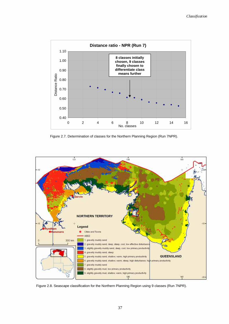
Classification
37
Figure 2.7. Determination of classes for the Northern Planning Region (Run 7NPR).
Figure 2.8. Seascape classification for the Northern Planning Region using 9 classes (Run 7NPR).
Distance ratio - NPR (Run 7)
0.40
0.50
0.60
0.70
0.80
0.90
1.00
1.10
0 2 4 6 8 10 12 14 16 No. classes
Dis
tanc
e R
atio
8 classes initially chosen, 9 classes finally chosen to
differentiate class means further
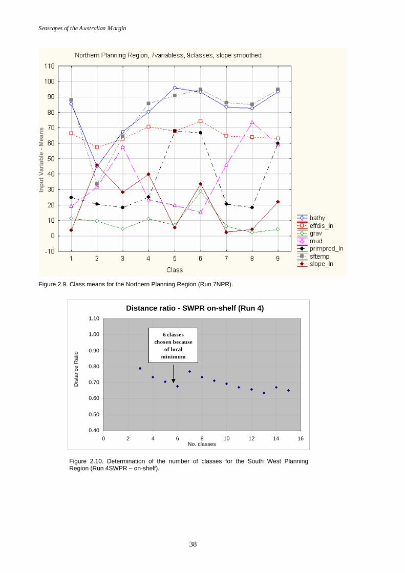
Seascapes of the Australian Margin
38
Figure 2.9. Class means for the Northern Planning Region (Run 7NPR).
Figure 2.10. Determination of the number of classes for the South West Planning Region (Run 4SWPR – on-shelf).
Distance ratio - SWPR on-shelf (Run 4)
0.40
0.50
0.60
0.70
0.80
0.90
1.00
1.10
0 2 4 6 8 10 12 14 16 No. classes
Dis
tanc
e R
atio
6 classes chosen because
of local minimum
Inpu
t Var
iabl
e - M
eans
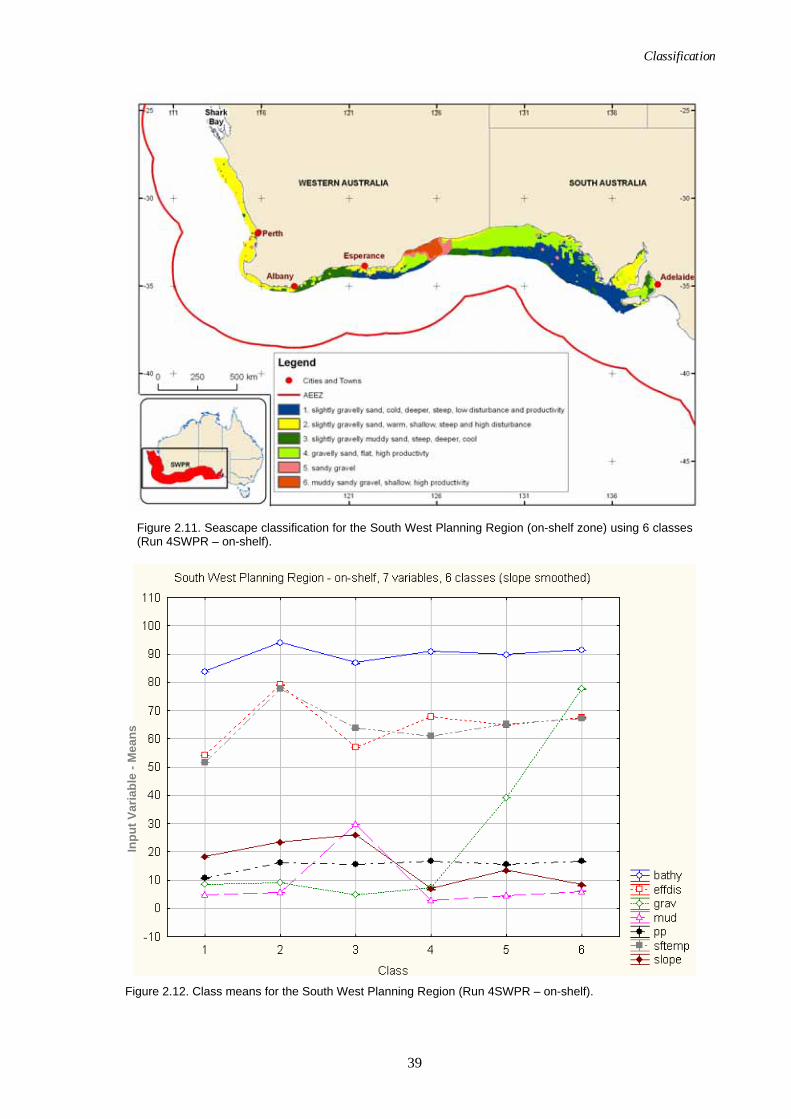
Classification
39
Figure 2.11. Seascape classification for the South West Planning Region (on-shelf zone) using 6 classes (Run 4SWPR – on-shelf).
Figure 2.12. Class means for the South West Planning Region (Run 4SWPR – on-shelf).
Inpu
t Var
iabl
e - M
eans
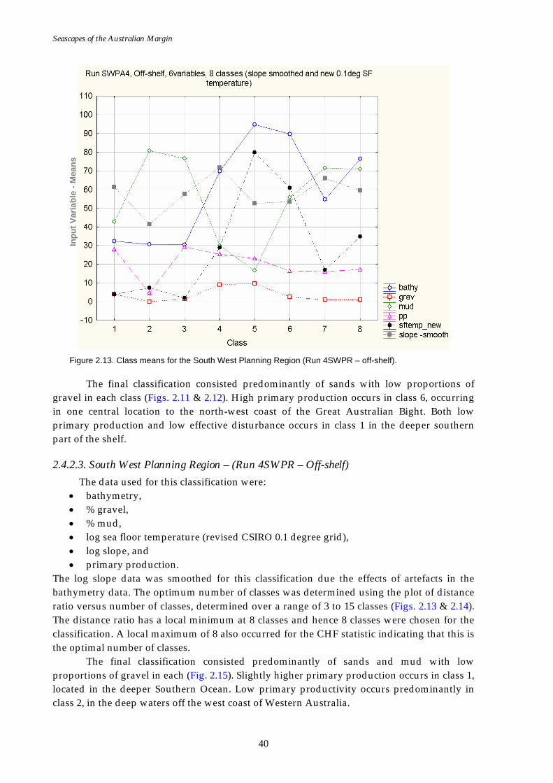
Seascapes of the Australian Margin
40
Figure 2.13. Class means for the South West Planning Region (Run 4SWPR – off-shelf).
The final classification consisted predominantly of sands with low proportions of gravel in each class (Figs. 2.11 & 2.12). High primary production occurs in class 6, occurring in one central location to the north-west coast of the Great Australian Bight. Both low primary production and low effective disturbance occurs in class 1 in the deeper southern part of the shelf.
2.4.2.3. South West Planning Region – (Run 4SWPR – Off-shelf) The data used for this classification were:
• bathymetry, • % gravel, • % mud, • log sea floor temperature (revised CSIRO 0.1 degree grid), • log slope, and • primary production.
The log slope data was smoothed for this classification due the effects of artefacts in the bathymetry data. The optimum number of classes was determined using the plot of distance ratio versus number of classes, determined over a range of 3 to 15 classes (Figs. 2.13 & 2.14). The distance ratio has a local minimum at 8 classes and hence 8 classes were chosen for the classification. A local maximum of 8 also occurred for the CHF statistic indicating that this is the optimal number of classes.
The final classification consisted predominantly of sands and mud with low proportions of gravel in each (Fig. 2.15). Slightly higher primary production occurs in class 1, located in the deeper Southern Ocean. Low primary productivity occurs predominantly in class 2, in the deep waters off the west coast of Western Australia.
Inpu
t Var
iabl
e - M
eans

Classification
41
Figure 2.14. Determination of the number of classes for the South West Planning Region (Run 4SWPR – off-shelf).
Figure 2.15. Seascape classification for the South West Planning Region (off-shelf zone) using 8 classes (Run 4SWPR – off-shelf).
Distance ratio - SWPR off-shelf (Run 4)
0.45
0.50
0.55
0.60
0.65
0.70
0.75
0 2 4 6 8 10 12 14 16 No. classes
Dis
tanc
e R
atio
8 classes
chosen because of local
minimum
Seascapes of the Australian Margin
42
2.5. DISCUSSION
2.5.1. General Discussion of Results The seascape datasets comprise integrated ecologically meaningful physical properties that represent potential distributions of various seabed habitats. Each seascape area corresponds to an area of similar biophysical properties and, by association, habitats and biological communities.
A total of 9 seascapes were defined for the NPR, which is comprised entirely of shelf (<200 m) environments, while only 6 seascapes were defined on the shelf for the SWPR. While we cannot discount the influence of data density on the composition of the final seascapes, this result implies that seabed environments in the north are potentially more diverse than those in the south.
In the NPR, the seascapes form a concentric pattern in the Gulf of Carpentaria which corresponds to increasing mud concentrations towards the central west of the gulf. A key feature of the seascapes in the gulf and on the coastal zone of Gove Peninsula and the Coburg Peninsula and is the location of Seascape 9 “slightly gravelly mud, shallow, warm, high primary productivity” at the mouths of the major rivers, which corresponds to distal delta deposits. Seascape 4 “gravelly muddy sand, steep” corresponds to relatively steep regions of the seabed such as the submerged reef margins in the southern gulf (cf. Harris et al., 2004), submarine canyons in the Arafura Sea, and Sahul Banks west of Bathurst Island. In the Arafura Sea, Seascape 8 “slightly gravelly sand, low primary productivity” corresponds to a region of relatively high terrigenous mud concentrations (Jongsma, 1974). Seascape 5 “gravelly muddy sand, shallow, warm, high primary productivity” defines a relatively contiguous coastal region in the Gulf of Carpentaria defined by warm water and elevated primary productivity. The latter property we treat with caution as the elevated values are more likely associated with high coastal turbidity from wave activity (high effective disturbance) and possibly seabed reflectance. Despite this, this seascape defines a distinct region of probable low light and disturbance, thus influencing the seabed biota. Seascape 6 is the equivalent region in the Joseph Bonaparte Gulf, but is characterised by a high level of effective disturbance and relatively coarse-grained sediments resulting from strong tidal currents associated with large tides (>4 m) and narrow coastal passages between islands. Seascape 9, located the Arafura Sea characterises a coastal region with relatively fine-grained sediments and reduced effective disturbance (tide and wave currents), with likely influence from the muddy facies located in the central Arafura Sea (Seascape 8). Seascapes 2 “gravelly muddy sand, deep, steep, cool, low effective disturbance” and 3 “slightly gravelly muddy sand, deep, cool, low primary productivity” characterise the deepest regions of the NPR, where water temperatures are much cooler and the effective disturbance is lower due to the greater water depths. Lower water temperatures are probably also influenced by up-welling onto the shelf from the Arafura Depression (cf. Harris et al., 2005). Cool-water coral species observed at relatively shallow water depths would seem to support this assertion (Logan et al., 2006).
An alternative seabed classification for the Northern Planning Region has been undertaken by Rochester et al. (2007) (Fig. 2.16). Importantly, this classification was based not only on physical data (e.g., sedimentology, bathymetry) but also used biological data (demersal fish, invertebrates) in reaching an optimal solution of 9 clusters. Moreover, the clustering methodology used in the Rochester et al. (2007) classification was different to that used by GA. While the GA seascape classification results in more spatial heterogeneity of the

Classification
43
Figure 2.16. Environmental cluster regions for the Northern Planning Region as defined by Rochester et al., (2007).
potential seabed habitats, the GA and Rochester et al. (2007) classifications provide broadly similar spatial distributions of the classes. Larger, more-contiguous classes occur in the Gulf of Carpentaria and smaller less-contiguous classes occur in the Arafura Sea and Joseph Bonaparte Gulf. Comparison of the classifications shows that Seascape 4 “gravelly muddy sand, steep” in the GA classification and Cluster 4 of the Rochester et al. (2007) classification have very similar distributions. The same is evident for Seascape 2 “gravelly muddy sand, deep, steep, cool, low effective disturbance” and Cluster 1, Seascape 6 “gravelly muddy sand, shallow, warm, steep, high disturbance, high primary productivity” and Cluster 8, as well as Seascape 8 “slightly gravelly sand, low primary productivity” and Cluster 3. The main difference is that the Rochester et al. (2007) classification shows slightly more diversity along the coast and inner shelf of the Gulf of Carpentaria, while the GA classification shows more differentiation in the central regions. The similarity of the two biophysical classifications for the Northern Planning Region indicates that the seascapes method provides a reasonably robust representation of the seabed environments and biota at a broad scale.
In the SWPR, most spatial heterogeneity in the seascapes occurs on the shelf between Albany and Esperance. However, a key feature of the shelf seascape distributions is the distinct division between seabed environments on the western and southern margins. The west is dominated by Seascape 2 “slightly gravelly sand, warm, shallow, steep and high disturbance” while Seascapes 1 “slightly gravelly sand, cold, deeper, steep, low disturbance and productivity” and 4 “gravelly sand, flat, high productivity” occupy most of the southern margin. This partitioning between the seascapes coincides with warmer seafloor temperatures and shallower depths, but also broadly corresponds with a change in sediment facies dominated
Seascapes of the Australian Margin
44
by algal/coralline grains on the western margin to sediment dominated by molluscan-foraminifera and bryozoan grains on the southern margin (James et al., 1997, 1999).
There is also a prominent inner-shelf/outer-shelf division in the seascapes, with Seascapes 1 and 4 bisecting much of the southern shelf (Fig. 2.11). The partitioning of the shelf environments as depicted by these two seascapes reflects an offshore increase in mud concentrations (Potter et al., in press), increase in primary productivity, and decrease in sea floor temperature. Seascape 1 is also characterised by lower disturbance from the predominant swell waves due to the greater water depths. This shelf parallel distribution in the seascapes corresponds to a shelf-parallel distribution in the surface sediment facies from inner-shelf bryozoan and bivalve sands to mid- and outer-shelf bryozoan and foraminiferal sand (James et al., 2001).
Another feature of the shelf of the southern margin is the presence of a large patch of sediment with high gravel concentrations. This area is the largest zone of gravel on the SWPR (Potter et al., in press). This region does not correspond to a significant change in the composition of the sediments but is a site of active carbonate production on the shelf (James et al., 2001).
In the SWPR, off the shelf, most heterogeneity in the seascapes occurs on the slope, with a shore-parallel distribution. The seascapes on the slope (4-8) are present on both the west and southern margins, with Seascape 5 “gravelly mud, shallow and warm” being continuous along the margins. These seascape distributions imply that the physical environments on the slope between the west and southern margins are similar. Broadly, seascapes 6 “slightly gravelly muddy sand, shallow and warm”, 7 “slightly gravelly muddy sand, steep”, and 8 “slightly gravelly muddy sand” correspond to regions where the slope has been incised by submarine canyons. These regions also correspond to known up-welling zones and active carbonate production on the shelf (James et al., 2001). The shore-parallel zonation of the slope appears to mostly coincide with increasing mud concentrations with water depth (Potter et al., in press). On the abyssal plain / deep ocean floor (AP/DOF) the seascapes are more homogeneous and contiguous. Interestingly, the strong west-south differentiation shown by the seascapes on the shelf is also apparent in the seascapes on the AP/DOF, with the seabed of the Perth Abyssal Plain (Seascape 1 “slightly gravelly muddy sand, high primary productivity, deep and cool”) being different to the seabed on the Southern Ocean (2 “slightly gravelly muddy sand, flat, low primary productivity, deep and cool” & 3 “slightly gravelly mud, high primary productivity, deep and cool”). Seascape 1 on the AP/DOF and 5 on the slope correspond to regions of relatively high mud concentrations (Potter et al., in press) and year-round down-welling and off-shelf sediment transport from the outer shelf-upper slope (James et al., 2001).
2.5.2. Potential Improvements The extent and distribution of raw seabed data is the most fundamental factor controlling the ultimate quality of the output seascape datasets. Increasing the quantity and quality of the input data will reduce the potential for artefacts to appear in the derived grids that could influence the final classifications. Increasing the data density will also improve the degree to which the input data represent the actual spatial distribution of seabed properties. GA has strict data quality assurance processes in place, but given that data for the Australian EEZ are still relatively sparse, a program is currently underway to collect and collate new samples, focussed on those areas of poorest data quality and/or density. If data density
Classification
45
increases enough it may be possible to decrease the cell grid size, and portray the seabed properties at a much better spatial resolution than is currently possible.
As such, the seascape datasets produced so far are not intended to provide highly detailed, local habitat information. The input cell size for these iterations is 0.01° which means that every cell covers an area of approximately 1 km2 and hence all datasets comprise an average value for that area of seabed. We believe that the outputs provide a broad guide to potential habitats at the sub-IMCRA scale (IMCRA Technical Group, 1998). Further data collection should be a priority to ensure that the very best interpolations and predictions can be made for the seabed.
It is also a long term aim to improve the accuracy of the input datasets through refinement of the methods used to interpolate the raw data points into input grids. In this analysis, the Inverse Distance Weighted method has been employed to ensure that the raw point values are preserved in the grid. However, there are many spatial interpolation methods available that use a variety of mathematical functions that are yet to be fully explored in the seascape classification procedure.
One aspect of the classification procedure that could be reviewed is the use of the unsupervised classification versus a supervised classification which permits more influence by the user in creating the final seascapes. A supervised classification can be useful if the user knows something about the relationships between the variables, allowing the application of scientific-based knowledge to be incorporated into the classification. For example, scientific knowledge can be introduced to help guide the classification through differential weighting of variables known to have strong associations which can affect their contribution(s) to the final classification. Despite this, the supervised classification methodology runs the risk of weighting variables inappropriately or inaccurately. Unlike the unsupervised classification where the lack of user input creates its integrity, the user input in a supervised classification provides meaning to the selection of class breaks. Conversely, without rigorous testing of processes and input data, increased user input can potentially have adverse effects such as:
• Application of scientific theory that is not accurate or not accurate for the area being investigated that causes the classification of data into clusters that are not representative or true to the real environment;
• Assignment of incorrect weightings to each (or combinations of) variable(s); and • Inclusion of user defined breaks in classes that result in the loss of naturally defined
breaks which are just as useful and meaningful as those described by the user. It is clear that where used appropriately, the inclusion of crucial scientific knowledge
can lead to more robust and meaningful seascapes. Ultimately, any classification should be supported with rigorous field testing or ground truthing to ensure that the classification produces defensible and reliable solutions.
2.6. CONCLUSION The seascape maps provide 100% spatial coverage based on an objective, multivariate statistical analysis of marine environmental data that define key attributes of the seabed. This approach offers essential information for managers and stakeholders who are involved with designing Australia’s national MPA system. Confidence in the process is enhanced by this reproducible, science-based approach for classifying seabed environments and thus identifying conservation priorities.

Seascapes of the Australian Margin
46
Importantly, a seascapes approach is not a replacement for direct sampling and mapping of seabed biodiversity. Areas indicated by the seascapes to be high in biodiversity based on physical surrogates must be validated by field surveys. Seascapes and the physical and biophysical data upon which they are based are useful complementary means for identifying locations where biodiversity conservation can be optimised when designing an MPA system, and to augment and provide surrogates for biological data.
The creation of the seascapes represents one method of overcoming the large biodiversity information gap that otherwise exists for most of the AEEZ, and therefore provides a degree of confidence for managers and stakeholders. The spatial analysis methods outlined in this section are part of a larger program presently underway at Geoscience Australia that will have applications to conservation planning and management of the AEEZ in future.

47
PART 3 – Uncertainty Analysis and Methodology Verification
3.1. INTRODUCTION In any attempt to describe components of the real world using models or classifications of data it is essential that a suitable validation process is undertaken, and that uncertainty is described.
Three methods were identified that could be used to validate the classification method presented in Part 2:
1. Application of a different classification method using the same data to ensure that the method is robust;
2. Comparison between seascape classes and sampled biophysical data (collected in previously non-sampled areas) to ensure that the classes defined by the seascape classification are depicting an accurate representation of what actually occurs on the ocean floor; and
3. Collation and analysis of benthic biotic survey data to determine if the species composition is distinguishable from one seascape class to the next.
The technique chosen to assess the validity of the seascape method was the application of another classification method to the same input data (Method 1). The second classification using Fuzzy c-means was undertaken by the University of Tasmania and was used to verify that: 1) the number of classes selected was the same for both methods, and 2) the final output classifications showed similar patterns and class boundaries.
This validation methodology was chosen initially over the other two methods because it could be undertaken without the requirement of further data collection. Additionally, the fuzzy c-means classification has an uncertainty analysis component. It was therefore possible to both verify the unsupervised crisp classification method and define areas of uncertainty in the classification.
Part 3 of this report describes the application and results from the unsupervised, fuzzy c-means classification and contrasts these results with those gained from the initial classification approach. Validation methods two and three above have been identified as future requirements, particularly the application of method three to further justify the use of seascape classification as a method of identifying seabed habitats and predicting potential biodiversity.
3.2. AIM The main aim is to compare and contrast results from two different classification methods to ensure that the unsupervised crisp classification method developed by GA to create the seascapes was robust and produced reliable results. The second aim is to identify areas of uncertainty in the seascape boundaries to target future work.
3.3. METHODOLOGY
3.3.1. Study Area The study area selected includes coastal waters off Tasmania and Victoria (Fig. 3.1).
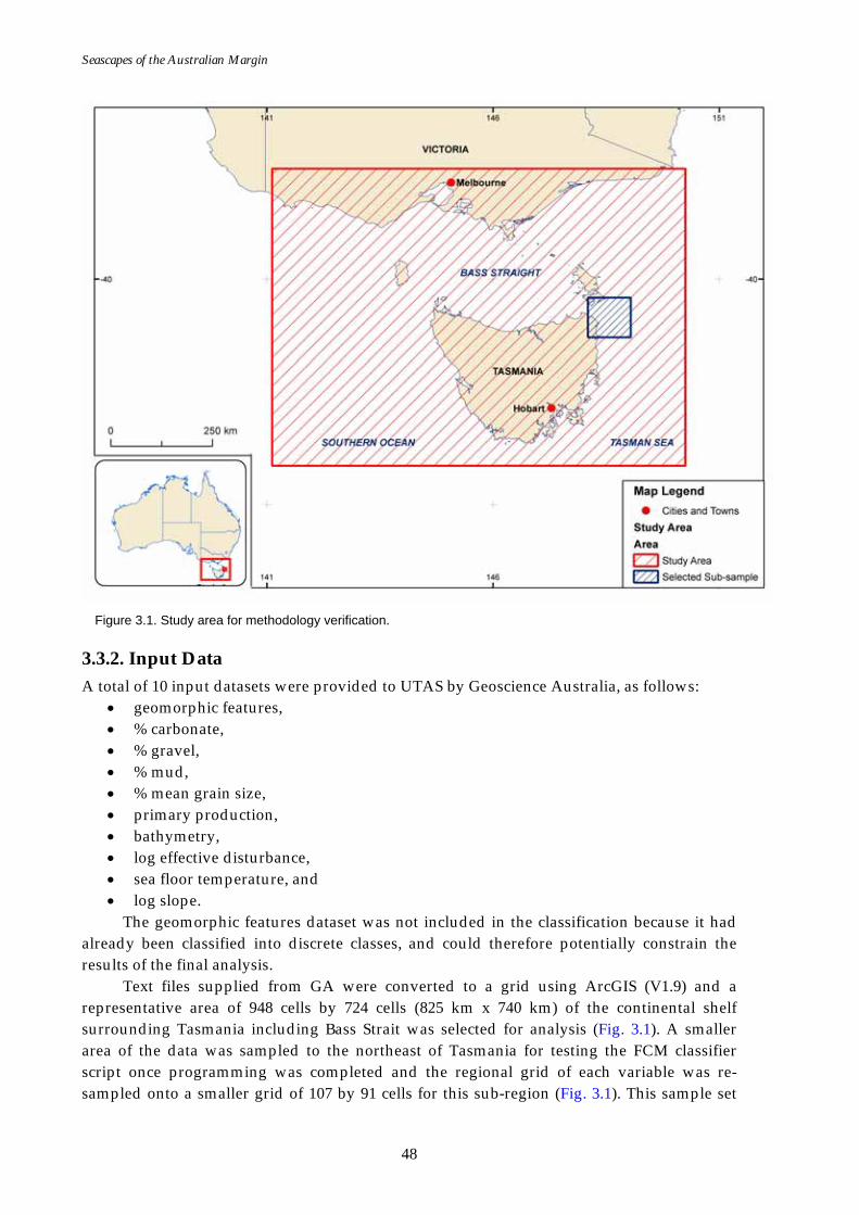
Seascapes of the Australian Margin
48
Figure 3.1. Study area for methodology verification.
3.3.2. Input Data A total of 10 input datasets were provided to UTAS by Geoscience Australia, as follows:
• geomorphic features, • % carbonate, • % gravel, • % mud, • % mean grain size, • primary production, • bathymetry, • log effective disturbance, • sea floor temperature, and • log slope.
The geomorphic features dataset was not included in the classification because it had already been classified into discrete classes, and could therefore potentially constrain the results of the final analysis.
Text files supplied from GA were converted to a grid using ArcGIS (V1.9) and a representative area of 948 cells by 724 cells (825 km x 740 km) of the continental shelf surrounding Tasmania including Bass Strait was selected for analysis (Fig. 3.1). A smaller area of the data was sampled to the northeast of Tasmania for testing the FCM classifier script once programming was completed and the regional grid of each variable was re-sampled onto a smaller grid of 107 by 91 cells for this sub-region (Fig. 3.1). This sample set
Uncertainty and Validation
49
was generated to test the FCM classifier script as the processing time required for the Tasmanian regional data set was much greater (x10).
3.3.3. Classification Methodology
3.3.3.1. Fuzzy c-means
In the initial unsupervised crisp classification method was chosen to ensure that bias was limited. The unsupervised approach was also applied in the Fuzzy c-means analysis to ensure that the two methods were comparable (both based on statistical analysis of the data and not driven by expert opinion).
Unlike the crisp classification approach, the fuzzy c-means classification methodology can describe the variation inherent in biophysical datasets. The fuzzy c-means method is applied to explore the data and define class boundaries for a user-defined number of classes.
3.3.3.2. Cluster Validation
The selection of the optimal number of clusters and location of the best class boundaries is a key component of unsupervised classifications. For fuzzy clustering there are a number of cluster validation methods reported in the literature, including; XB index (Xie & Beni, 1991), and Bezdek’s PE and PC indices (Bezdek, 1974; 1992, Bezdek et al., 1984). In this study seven cluster validity measures were used in conjunction with the fuzzy c-means algorithm (FCM); Partition Coefficient (PC), Partition Entropy (PE), Monotonic Partition Coefficient (MPC), Fuzzy Hyper Volume (FHV), Xie-Beni (XBm), PBMF and the Partition coefficient and exponential separation index (PCAES).
All of these indices are either the most cited or the newest validity measures proposed in the literature for fuzzy clustering. All of these indices have the common objective of finding a good estimate of a cluster number so that each one of the clusters is compact and separated from the others. A brief description of each validation index is included, with full equations for each, in Appendix E.
There are two components to the cluster validity measures applied in this study: 1) the compactness, which quantifies how compact the clusters are (the more compact the better), and 2) the distance between cluster centroids, which quantifies the distance between the cluster centroids in feature space (the larger and the further the centroids are apart, the better the separation). The XBm, PBMF, and PCAES are a combination of these two measures and vary only slightly in their definitions. PE, PC, MPC, and FHV only try to model the compactness of the clusters.
In this analysis, two scenarios for clustering were used: the XBm cluster validity measure and the PCAES index. The PCAES index differs slightly to the others in that it measures the potential to see whether an identified cluster has the ability to be a good cluster or not. Under this criterion, a noisy point would not have enough potential to form a cluster. The XBm cluster validity measure was chosen as it produces a number of classes that is the closest representation to the number of classes generated by the unsupervised crisp classification methodology. The two cluster validation indexes used are detailed below. A full description of the relevant equations is provided in Appendix E.
The XBm index was developed by Xie and Beni (1991) and identifies the optimal number of clusters through selection of the minimum index value. A large Partition Coefficient and Exponential separation index (PCAES) (Wu & Yang, 2005) means that each of
Seascapes of the Australian Margin
50
the c clusters is compact and separated from the other clusters. This is a new validity index for fuzzy clustering.
3.3.4. Fuzzy Classification for Selected Class Numbers The original script for fuzzy c-means classification (Burrough et al., 2000) was programmed first using Python (2.1), but due to computational effort it was reprogrammed in IDL. Seven validation indices were chosen to perform the initial partitioning of the datasets. The cluster validation measures generates plots showing the number of iterations the clustering algorithm needed to run to generate clusters that were compact and well distributed. This is a controlled procedure where the number of iterations is first established by the user. Between 2 and 40 iterations were suggested by the convergence graphs. From the plots generated by the validation indices we could select the optimal number of classes from either the minimum or maximum number of suggested classes to be input into the FCM Classifier.
The fuzzy c-means algorithm is described in detail in Burrough and McDonnell (1998) and Burrough et al. (2000). The Seascapes classification was regenerated for the optimum number of classes using both the class numbers suggested by the PCAES index and the XBm index. The hardclass maps were then compared to the seascape classification generated from the unsupervised crisp classification. The FCM classifier generates three main results: 1) a hardclass map, 2) a confusion map, and 3) a membership map for each of the classes.
3.3.5. Uncertainty Analysis – Confusion Maps An additional output from the fuzzy classification is a confusion index map (CI Map), which gives an indication of how confident the model is that each data point has been placed in the correct class. In this way confusion between overlapping classes (where the fuzziness occurs) can be explained as expressed by Burrough et al. (1997), as follows:
CI = (µ(max-1)i) / (µmaxi) (Eq. 3.1)
where µmaxi is the membership value of the class with the maximum µk at site i and µmax-1 is the second largest membership value at the same site.
The values of the CI map are scaled between 0 and 1. If the confusion index approaches 1, then both µi values are near equal and there is confusion about the class to which the site nearly belongs (high uncertainty and low confidence). If the confusion index approaches 0, then both µi values are not equal and there is little overlap, one class dominates and there is little confusion (high confidence, low uncertainty) (Burrough et al., 2000). There may be regions where µi and µj values are very similar for multiple points, in which case confusion exists because it would be hard to determine which class dominates.
3.3.5.1. Validation of Cluster Selection Using Confusion Maps
CI maps were created primarily to validate the process of class selection (cluster validation). As described above, different cluster validation techniques identify the optimal number of classes using various methods, and consequently the results are often greatly varied. In this study numerous cluster validity approaches were applied, with finally two cluster validation techniques selected for further analysis. CI Maps were created for optimal number of classes as indicated by these two cluster validation methods. The CI maps provide an immediate visual and statistical representation of the confidence of the classifications, and are then used to select the number of classes that causes the least confusion.
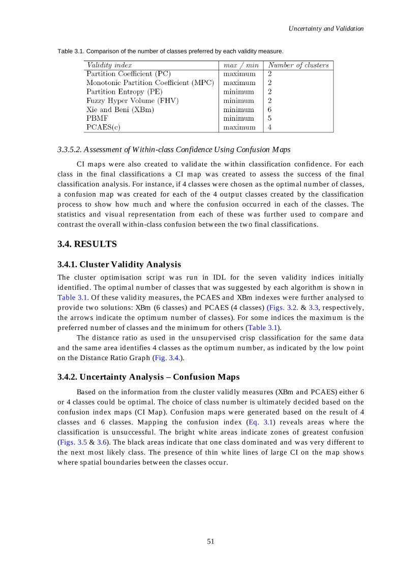
Uncertainty and Validation
51
Table 3.1. Comparison of the number of classes preferred by each validity measure.
3.3.5.2. Assessment of Within-class Confidence Using Confusion Maps
CI maps were also created to validate the within classification confidence. For each class in the final classifications a CI map was created to assess the success of the final classification analysis. For instance, if 4 classes were chosen as the optimal number of classes, a confusion map was created for each of the 4 output classes created by the classification process to show how much and where the confusion occurred in each of the classes. The statistics and visual representation from each of these was further used to compare and contrast the overall within-class confusion between the two final classifications.
3.4. RESULTS
3.4.1. Cluster Validity Analysis The cluster optimisation script was run in IDL for the seven validity indices initially identified. The optimal number of classes that was suggested by each algorithm is shown in Table 3.1. Of these validity measures, the PCAES and XBm indexes were further analysed to provide two solutions: XBm (6 classes) and PCAES (4 classes) (Figs. 3.2. & 3.3, respectively, the arrows indicate the optimum number of classes). For some indices the maximum is the preferred number of classes and the minimum for others (Table 3.1).
The distance ratio as used in the unsupervised crisp classification for the same data and the same area identifies 4 classes as the optimum number, as indicated by the low point on the Distance Ratio Graph (Fig. 3.4.).
3.4.2. Uncertainty Analysis – Confusion Maps Based on the information from the cluster validly measures (XBm and PCAES) either 6
or 4 classes could be optimal. The choice of class number is ultimately decided based on the confusion index maps (CI Map). Confusion maps were generated based on the result of 4 classes and 6 classes. Mapping the confusion index (Eq. 3.1) reveals areas where the classification is unsuccessful. The bright white areas indicate zones of greatest confusion (Figs. 3.5 & 3.6). The black areas indicate that one class dominated and was very different to the next most likely class. The presence of thin white lines of large CI on the map shows where spatial boundaries between the classes occur.
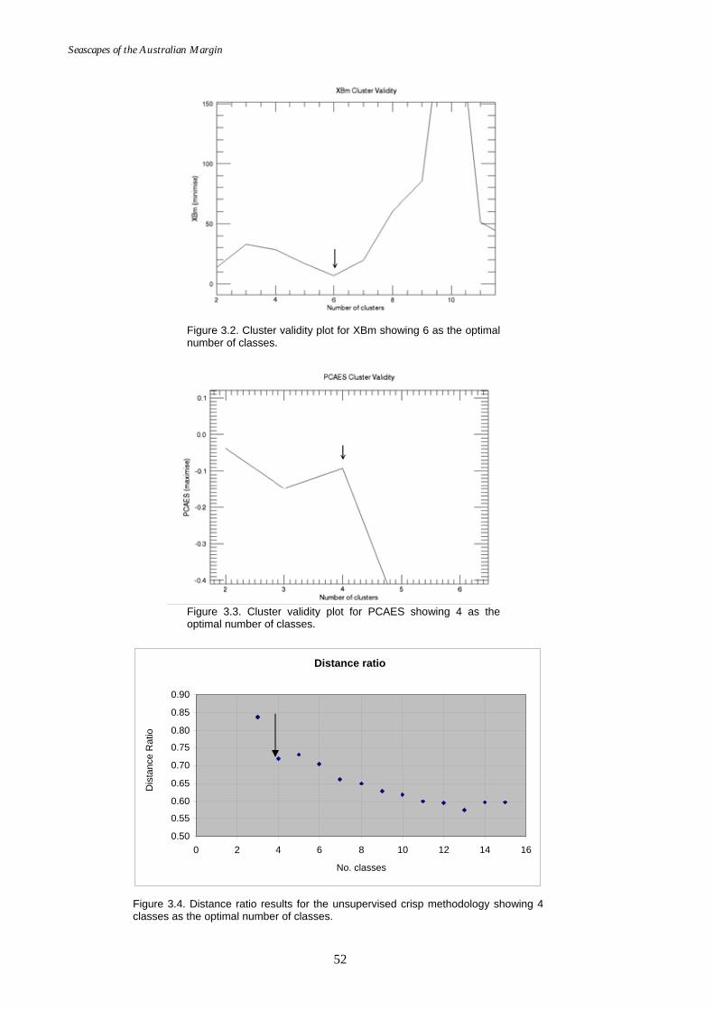
Seascapes of the Australian Margin
52
Figure 3.2. Cluster validity plot for XBm showing 6 as the optimal number of classes.
Figure 3.3. Cluster validity plot for PCAES showing 4 as the optimal number of classes.
Figure 3.4. Distance ratio results for the unsupervised crisp methodology showing 4 classes as the optimal number of classes.
Distance ratio
0.50 0.55 0.60 0.65 0.70 0.75 0.80 0.85 0.90
0 2 4 6 8 10 12 14 16 No. classes
Dis
tanc
e R
atio
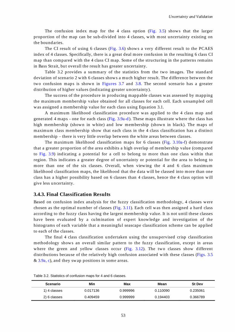
Uncertainty and Validation
53
The confusion index map for the 4 class option (Fig. 3.5) shows that the larger proportion of the map can be sub-divided into 4 classes, with most uncertainty existing on the boundaries.
The CI result of using 6 classes (Fig. 3.6) shows a very different result to the PCAES index of 4 classes. Specifically, there is a great deal more confusion in the resulting 6 class CI map than compared with the 4 class CI map. Some of the structuring in the patterns remains in Bass Strait, but overall the result has greater uncertainty.
Table 3.2 provides a summary of the statistics from the two images. The standard deviation of scenario 2 with 6 classes shows a much higher result. The difference between the two confusion maps is shown in Figures 3.7 and 3.8. The second scenario has a greater distribution of higher values (indicating greater uncertainty).
The success of the procedure in producing mappable classes was assessed by mapping the maximum membership value obtained for all classes for each cell. Each unsampled cell was assigned a membership value for each class using Equation 3.1.
A maximum likelihood classification procedure was applied to the 4 class map and generated 4 maps - one for each class (Fig. 3.9a-d). These maps illustrate where the class has high membership (shown in white) and low membership (shown in black). The maps of maximum class membership show that each class in the 4 class classification has a distinct membership – there is very little overlap between the white areas between classes.
The maximum likelihood classification maps for 6 classes (Fig. 3.10a-f) demonstrate that a greater proportion of the area exhibits a high overlap of membership value (compared to Fig. 3.9) indicating a potential for a cell to belong to more than one class within that region. This indicates a greater degree of uncertainty or potential for the area to belong to more than one of the six classes. Overall, when viewing the 4 and 6 class maximum likelihood classification maps, the likelihood that the data will be classed into more than one class has a higher possibility based on 6 classes than 4 classes, hence the 4 class option will give less uncertainty.
3.4.3. Final Classification Results Based on confusion index analysis for the fuzzy classification methodology, 4 classes were chosen as the optimal number of classes (Fig. 3.11). Each cell was then assigned a hard class according to the fuzzy class having the largest membership value. It is not until these classes have been evaluated by a culmination of expert knowledge and investigation of the histograms of each variable that a meaningful seascape classification scheme can be applied to each of the classes.
The final 4 class classification undertaken using the unsupervised crisp classification methodology shows an overall similar pattern to the fuzzy classification, except in areas where the green and yellow classes occur (Fig. 3.12). The two classes show different distributions because of the relatively high confusion associated with these classes (Figs. 3.5 & 3.9a, c), and they swap positions in some areas.
Table 3.2. Statistics of confusion maps for 4 and 6 classes.
Scenario Min Max Mean St Dev
1) 4 classes 0.017136 0.999996 0.110090 0.235061
2) 6 classes 0.409459 0.999999 0.194403 0.366789
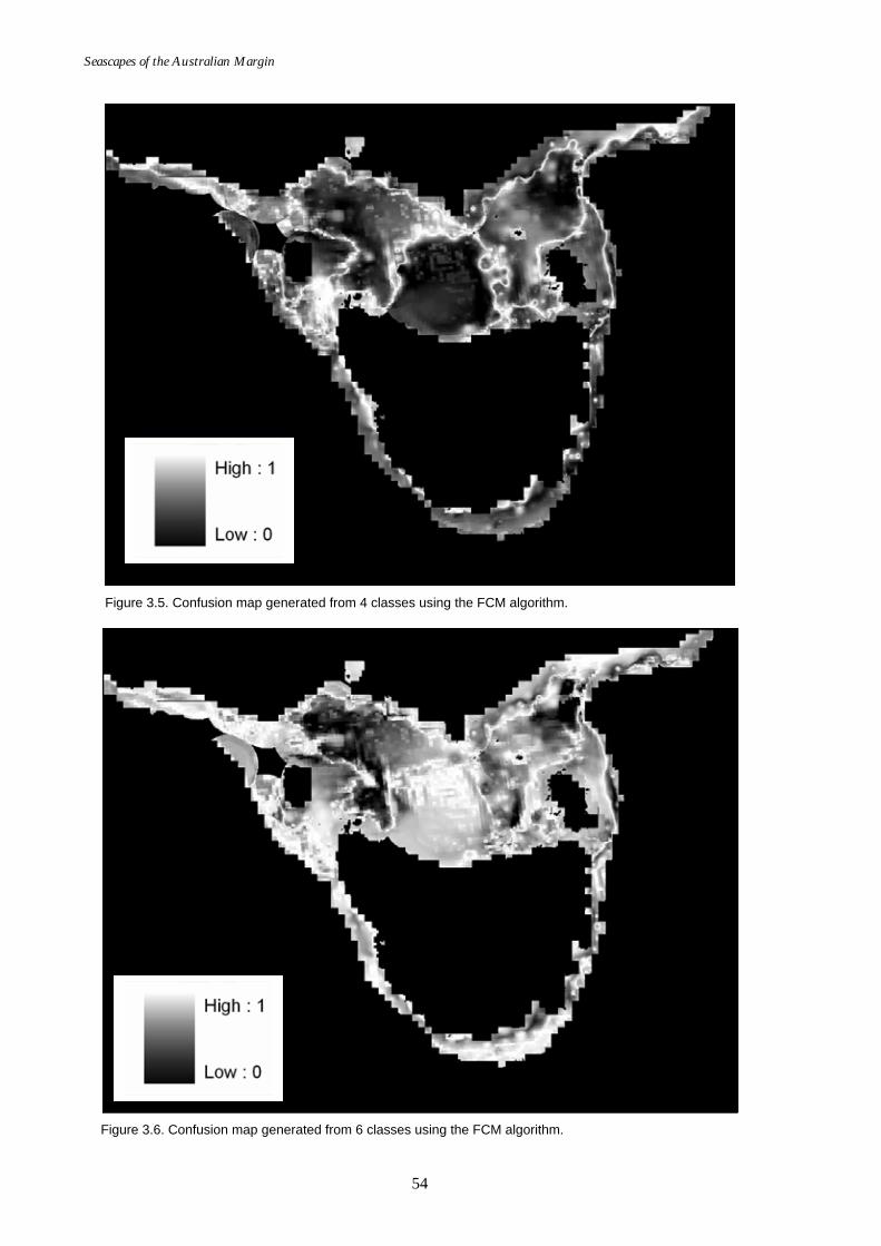
Seascapes of the Australian Margin
54
Figure 3.5. Confusion map generated from 4 classes using the FCM algorithm.
Figure 3.6. Confusion map generated from 6 classes using the FCM algorithm.

Uncertainty and Validation
55
Figure 3.7. Plot showing the frequency of data values for confusion map 4 classes.
Figure 3.8. Plot showing the frequency of data values for confusion map 6 classes.
3.5. DISCUSSION
3.5.1. General Discussion of Results Results from each of the cluster validity measures show that no single index can be used exclusively on the biophysical data to create the seascapes, given the interpolation methods used and the heterogenous data distributions. Sophisticated classification or interpolation methods do not result in continuity in the attributes or contiguity in geographical space if the distribution of the input data is very heterogenous across the study area. However, the two methods employed here to validate the seascape classification show that the fuzzy c-means approach can locate potential boundaries between multiple seabed properties and the membership of each grid cell to each seascape. The result is spatially contiguous and
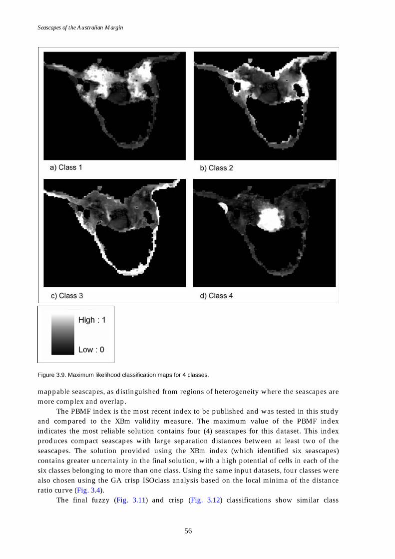
Seascapes of the Australian Margin
56
Figure 3.9. Maximum likelihood classification maps for 4 classes.
mappable seascapes, as distinguished from regions of heterogeneity where the seascapes are more complex and overlap.
The PBMF index is the most recent index to be published and was tested in this study and compared to the XBm validity measure. The maximum value of the PBMF index indicates the most reliable solution contains four (4) seascapes for this dataset. This index produces compact seascapes with large separation distances between at least two of the seascapes. The solution provided using the XBm index (which identified six seascapes) contains greater uncertainty in the final solution, with a high potential of cells in each of the six classes belonging to more than one class. Using the same input datasets, four classes were also chosen using the GA crisp ISOclass analysis based on the local minima of the distance ratio curve (Fig. 3.4).
The final fuzzy (Fig. 3.11) and crisp (Fig. 3.12) classifications show similar class
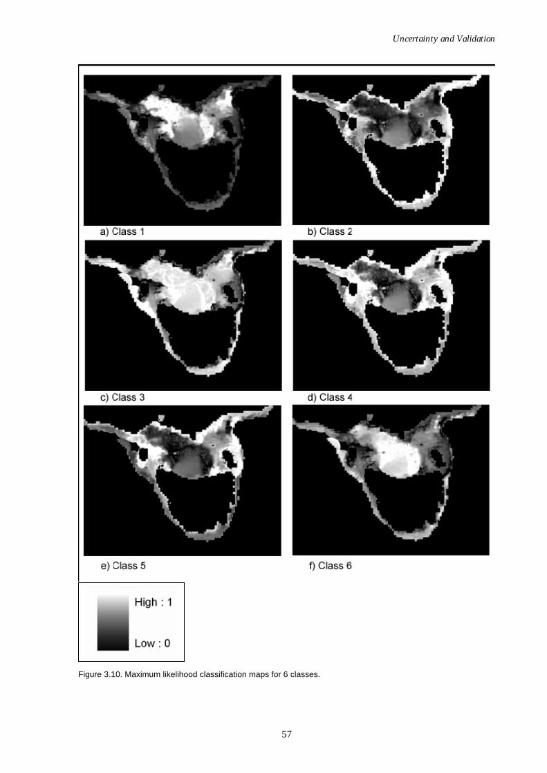
Uncertainty and Validation
57
Figure 3.10. Maximum likelihood classification maps for 6 classes.
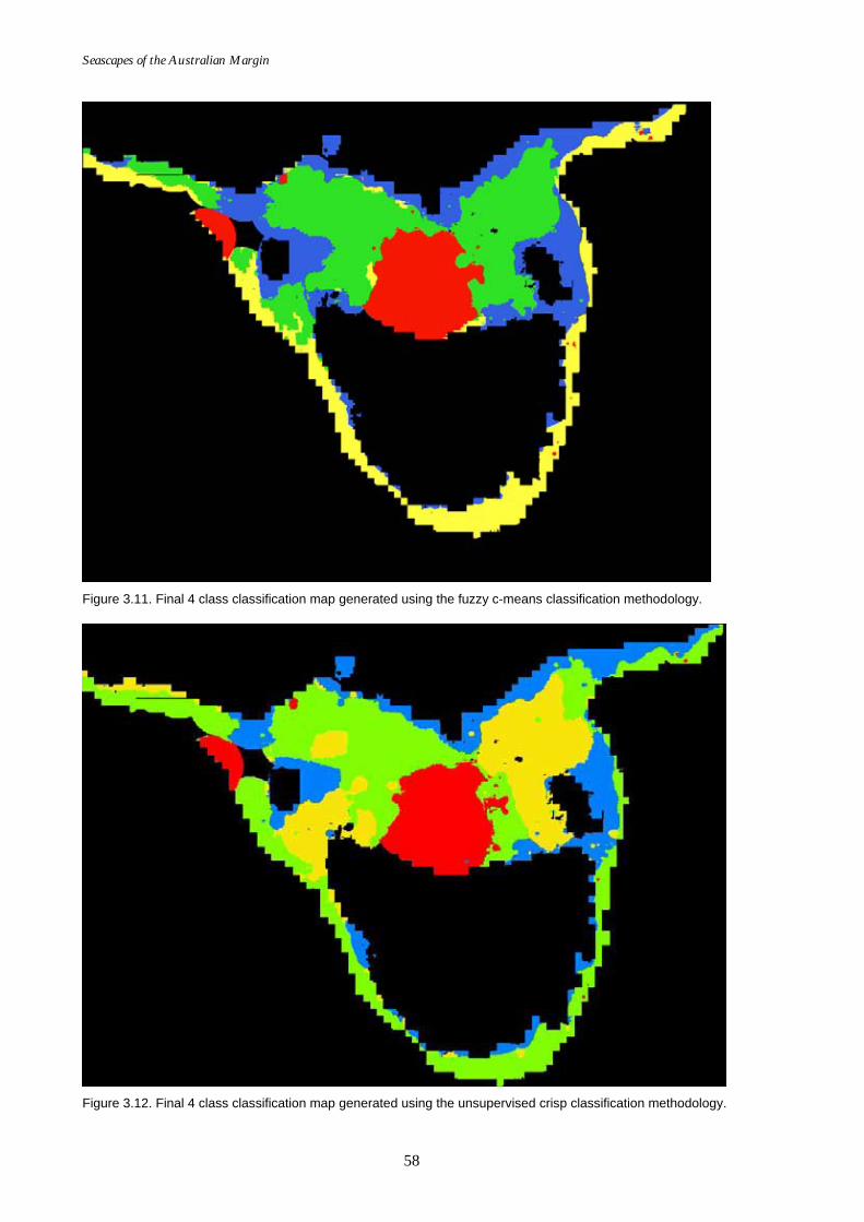
Seascapes of the Australian Margin
58
Figure 3.11. Final 4 class classification map generated using the fuzzy c-means classification methodology.
Figure 3.12. Final 4 class classification map generated using the unsupervised crisp classification methodology.
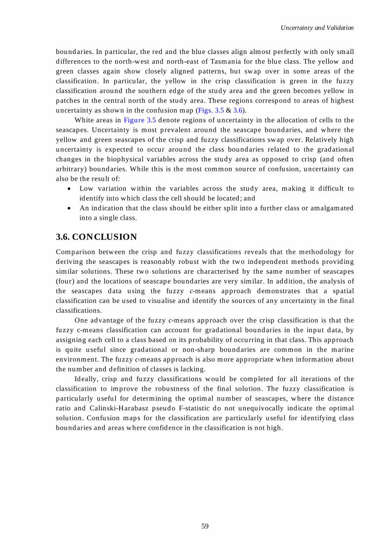
Uncertainty and Validation
59
boundaries. In particular, the red and the blue classes align almost perfectly with only small differences to the north-west and north-east of Tasmania for the blue class. The yellow and green classes again show closely aligned patterns, but swap over in some areas of the classification. In particular, the yellow in the crisp classification is green in the fuzzy classification around the southern edge of the study area and the green becomes yellow in patches in the central north of the study area. These regions correspond to areas of highest uncertainty as shown in the confusion map (Figs. 3.5 & 3.6).
White areas in Figure 3.5 denote regions of uncertainty in the allocation of cells to the seascapes. Uncertainty is most prevalent around the seascape boundaries, and where the yellow and green seascapes of the crisp and fuzzy classifications swap over. Relatively high uncertainty is expected to occur around the class boundaries related to the gradational changes in the biophysical variables across the study area as opposed to crisp (and often arbitrary) boundaries. While this is the most common source of confusion, uncertainty can also be the result of:
• Low variation within the variables across the study area, making it difficult to identify into which class the cell should be located; and
• An indication that the class should be either split into a further class or amalgamated into a single class.
3.6. CONCLUSION Comparison between the crisp and fuzzy classifications reveals that the methodology for deriving the seascapes is reasonably robust with the two independent methods providing similar solutions. These two solutions are characterised by the same number of seascapes (four) and the locations of seascape boundaries are very similar. In addition, the analysis of the seascapes data using the fuzzy c-means approach demonstrates that a spatial classification can be used to visualise and identify the sources of any uncertainty in the final classifications.
One advantage of the fuzzy c-means approach over the crisp classification is that the fuzzy c-means classification can account for gradational boundaries in the input data, by assigning each cell to a class based on its probability of occurring in that class. This approach is quite useful since gradational or non-sharp boundaries are common in the marine environment. The fuzzy c-means approach is also more appropriate when information about the number and definition of classes is lacking.
Ideally, crisp and fuzzy classifications would be completed for all iterations of the classification to improve the robustness of the final solution. The fuzzy classification is particularly useful for determining the optimal number of seascapes, where the distance ratio and Calinski-Harabasz pseudo F-statistic do not unequivocally indicate the optimal solution. Confusion maps for the classification are particularly useful for identifying class boundaries and areas where confidence in the classification is not high.
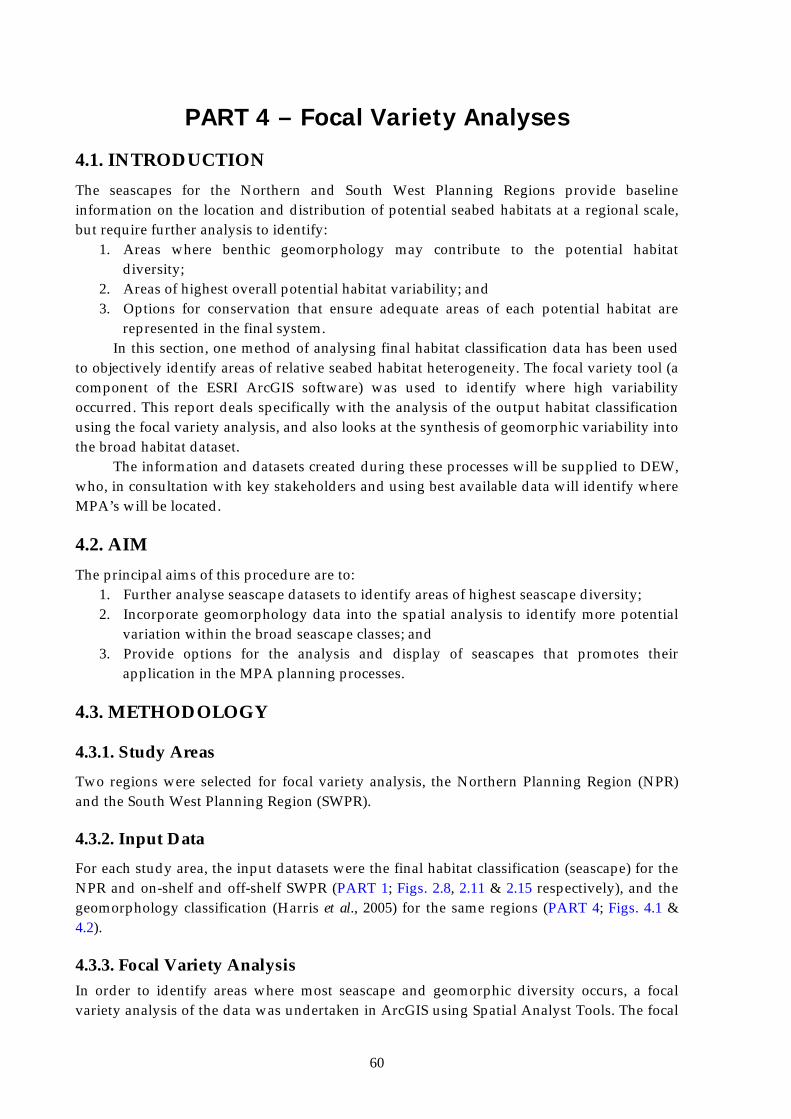
60
PART 4 – Focal Variety Analyses
4.1. INTRODUCTION The seascapes for the Northern and South West Planning Regions provide baseline information on the location and distribution of potential seabed habitats at a regional scale, but require further analysis to identify:
1. Areas where benthic geomorphology may contribute to the potential habitat diversity;
2. Areas of highest overall potential habitat variability; and 3. Options for conservation that ensure adequate areas of each potential habitat are
represented in the final system. In this section, one method of analysing final habitat classification data has been used
to objectively identify areas of relative seabed habitat heterogeneity. The focal variety tool (a component of the ESRI ArcGIS software) was used to identify where high variability occurred. This report deals specifically with the analysis of the output habitat classification using the focal variety analysis, and also looks at the synthesis of geomorphic variability into the broad habitat dataset.
The information and datasets created during these processes will be supplied to DEW, who, in consultation with key stakeholders and using best available data will identify where MPA’s will be located.
4.2. AIM The principal aims of this procedure are to:
1. Further analyse seascape datasets to identify areas of highest seascape diversity; 2. Incorporate geomorphology data into the spatial analysis to identify more potential
variation within the broad seascape classes; and 3. Provide options for the analysis and display of seascapes that promotes their
application in the MPA planning processes.
4.3. METHODOLOGY
4.3.1. Study Areas Two regions were selected for focal variety analysis, the Northern Planning Region (NPR) and the South West Planning Region (SWPR).
4.3.2. Input Data For each study area, the input datasets were the final habitat classification (seascape) for the NPR and on-shelf and off-shelf SWPR (PART 1; Figs. 2.8, 2.11 & 2.15 respectively), and the geomorphology classification (Harris et al., 2005) for the same regions (PART 4; Figs. 4.1 & 4.2).
4.3.3. Focal Variety Analysis In order to identify areas where most seascape and geomorphic diversity occurs, a focal variety analysis of the data was undertaken in ArcGIS using Spatial Analyst Tools. The focal
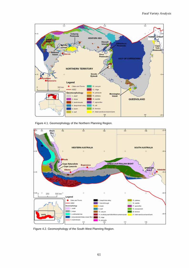
Focal Variety Analysis
61
Figure 4.1. Geomorphology of the Northern Planning Region.
Figure 4.2. Geomorphology of the South West Planning Region.
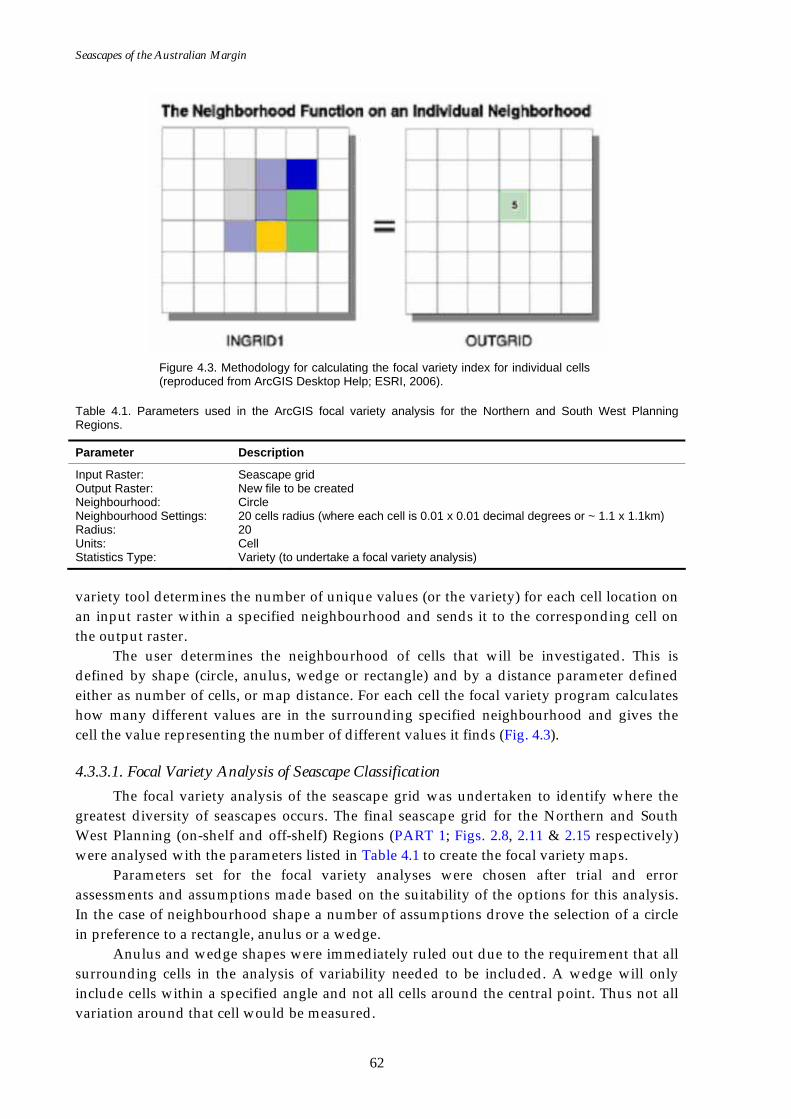
Seascapes of the Australian Margin
62
Figure 4.3. Methodology for calculating the focal variety index for individual cells (reproduced from ArcGIS Desktop Help; ESRI, 2006).
Table 4.1. Parameters used in the ArcGIS focal variety analysis for the Northern and South West Planning Regions.
Parameter Description
Input Raster: Output Raster: Neighbourhood: Neighbourhood Settings: Radius: Units: Statistics Type:
Seascape grid New file to be created Circle 20 cells radius (where each cell is 0.01 x 0.01 decimal degrees or ~ 1.1 x 1.1km) 20 Cell Variety (to undertake a focal variety analysis)
variety tool determines the number of unique values (or the variety) for each cell location on an input raster within a specified neighbourhood and sends it to the corresponding cell on the output raster.
The user determines the neighbourhood of cells that will be investigated. This is defined by shape (circle, anulus, wedge or rectangle) and by a distance parameter defined either as number of cells, or map distance. For each cell the focal variety program calculates how many different values are in the surrounding specified neighbourhood and gives the cell the value representing the number of different values it finds (Fig. 4.3).
4.3.3.1. Focal Variety Analysis of Seascape Classification The focal variety analysis of the seascape grid was undertaken to identify where the
greatest diversity of seascapes occurs. The final seascape grid for the Northern and South West Planning (on-shelf and off-shelf) Regions (PART 1; Figs. 2.8, 2.11 & 2.15 respectively) were analysed with the parameters listed in Table 4.1 to create the focal variety maps.
Parameters set for the focal variety analyses were chosen after trial and error assessments and assumptions made based on the suitability of the options for this analysis. In the case of neighbourhood shape a number of assumptions drove the selection of a circle in preference to a rectangle, anulus or a wedge.
Anulus and wedge shapes were immediately ruled out due to the requirement that all surrounding cells in the analysis of variability needed to be included. A wedge will only include cells within a specified angle and not all cells around the central point. Thus not all variation around that cell would be measured.
Focal Variety Analysis
63
An anulus can be set to omit one or many cells from the centre of the circle. In this study no central cells needed to be omitted, and the central point was considered important. Potentially the inside cell could have a different habitat type to the surrounding cells, and this variation would need to be shown in the final grid. If the central point was omitted from the analysis it could show no variation, even though it is itself different from surrounding cells. This would show up on a grid as a low variation point surrounded by high variation, when it should show up as all high variation.
In the case of the circle or square neighbourhood type, a circle was chosen because its appearance more closely represented natural features, without straight lines and corners. The natural boundaries of the features are predominantly curved, and a circle focal variety analysis better matches that pattern.
A radius of 20 cells was chosen after trials of 10, 15, 20 and 30 circle radii. It is possible to have extremely large radii in the focal variety analysis to include more cells in each neighbourhood. However, the larger the radius, the more variability each cell will have, and eventually distant variability will be included in the results displaying areas with high variability, when they are not particularly variable at a more local scale. Conversely, the values of 10 and 15 did not highlight the medium variability areas well. With cell radii set to 10 or 15, there was no connectivity between each isolated point of high variability. Therefore a final radius of 20 cells was chosen because it showed the highest variability areas and some broader patterns of variability without including areas of high variability driven by cells too distant from the central cell.
Running the focal variety analysis with these parameters will produce a new grid showing the variability (or heterogeneity) of the benthic habitat based on a circle radius of 20 cells.
4.3.3.2. Analysis of Geomorphology with Seascape Classifications Broad-scale geomorphology of the ocean floor (slope, terrace, basin etc), readily
mapped using bathymetric data, can provide within class differentiation of broad scale seabed or benthic habitats (Harris et al., 2003). Locations where seascapes and a range of geomorphic features intersect indicate high potential habitat variability, and therefore high potential biotic variability (Day & Roff, 2000).
The geomorphology dataset was analysed using the focal variety tool as described in section 3.3.1, with all parameters remaining the same. This produced a grid showing areas of high geomorphic variability.
The focal variety analysis outputs grids for seascapes and geomorphology were then scaled (so they were evenly weighted) and combined (addition) using the ArcToolbox/Spatial Analyst Tools/ Math/Plus Tool. For each cell the tool adds the value from the focal variety analysis of the seascapes to the focal variety of the geomorphology to give a total variability for the combined datasets.
The aim of this final dataset is to identify areas where there is a combination of high seascape variability and high geomorphic variability, and hence high potential biotic heterogeneity.
Seascapes of the Australian Margin
64
4.4. RESULTS
4.4.1. Focal Variety Analysis Results
4.4.1.1. Northern Planning Region – Seascapes The focal variety output grid of the 9 class seascape classification for the NPR has a
range of 1 through to 8, where 8 indicates that there are 8 different seascapes in the neighbourhood of that cell, and 1 indicates that there is only 1 seascape in the neighbourhood of that cell (Fig. 4.4).
The majority of the Torres Straight and the Gulf of Carpentaria Basin shows very low (dark blue; 1 seascape type in 20 km radius) seascape variation, and only moderate variation in the Arafura Sea area. High (orange; 6-7 seascapes) seascape variation occurs:
• On the southern coastal zone of the Arafura Sea; • On the southern coastal zone of the Gulf of Carpentaria; • East and west of the Wessell Islands continuing south east down the Gove Peninsula;
and • South and east of Groote Eylandt.
4.4.1.2. Northern Planning Region – Geomorphology Of the 21 classes of geomorphology represented in Australian waters, only 19 of these
classes are represented in the NPR. Here, the focal variety output grid of the 19 class geomorphology dataset has a range of 1 through to 8 (Fig. 4.5), where 8 indicates that there are 8 different geomorphology types in the neighbourhood of that cell, and 1 indicates that there is only 1 geomorphology type in the neighbourhood of that cell. The majority of the Gulf of Carpentaria Basin shows very low (dark blue; 1 seascape) variation of geomorphology, and only moderate variation to the west of Darwin.
High geomorphology variation occurs to the north of the Gove Peninsula in the Wessell Islands. Very high (orange; 6-7 seascapes) geomorphology variation occurs to the north of the Gove Peninsula in the Wessell Islands, around Groote Eylandt and to the north and east of Mornington Island in the south of the Gulf of Carpentaria. A large area of very high geomorphologic variation (red; 8 seascapes) occurs around the Wessell Islands.
4.4.1.3. Northern Planning Region – Combined Dataset In the NPR, the combination of the focal variety of geomorphology and seascapes has a
range of 2 through to 15, where 15 indicates that there is high combined seascape and geomorphic variability, and 2 indicates that there is low combined seascape and geomorphic variability (Fig. 4.6). The majority of the output grid has low variation and only moderate variation to the north-west of Darwin. High variation (orange, 11-13 seascapes) occurs:
• North of the Gove Peninsula in the Wessell Islands; • East and south of Groote Eylandt; and • North and east of Mornington Island in the south of the Gulf of Carpentaria.
The highest variation (red) occurs only in one small location off Cape Wilberforce.
4.4.1.4. South West Planning Region Off-shelf – Seascapes In the off-shelf zone of the SWPR, the focal variety output grid of the 8 class seascape
has a range of 1 through to 7 (Fig. 4.7). The majority of the focal variety grid shows very low
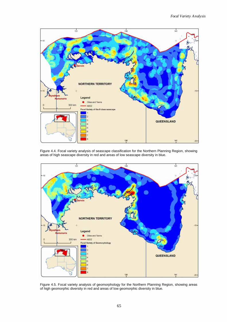
Focal Variety Analysis
65
Figure 4.4. Focal variety analysis of seascape classification for the Northern Planning Region, showing areas of high seascape diversity in red and areas of low seascape diversity in blue.
Figure 4.5. Focal variety analysis of geomorphology for the Northern Planning Region, showing areas of high geomorphic diversity in red and areas of low geomorphic diversity in blue.
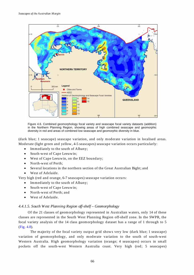
Seascapes of the Australian Margin
66
Figure 4.6. Combined geomorphology focal variety and seascape focal variety datasets (addition) in the Northern Planning Region, showing areas of high combined seascape and geomorphic diversity in red and areas of combined low seascape and geomorphic diversity in blue.
(dark blue; 1 seascape) seascape variation, and only moderate variation in localised areas. Moderate (light green and yellow, 4-5 seascapes) seascape variation occurs particularly:
• Immediately to the south of Albany; • South-west of Cape Leeuwin; • West of Cape Leeuwin, on the EEZ boundary; • North-west of Perth; • Several locations in the northern section of the Great Australian Bight; and • West of Adelaide.
Very high (red and orange, 6-7 seascapes) seascape variation occurs: • Immediately to the south of Albany; • South-west of Cape Leeuwin; • North-west of Perth; and • West of Adelaide.
4.4.1.5. South West Planning Region off-shelf – Geomorphology Of the 21 classes of geomorphology represented in Australian waters, only 14 of these
classes are represented in the South West Planning Region off-shelf zone. In the SWPR, the focal variety analysis of the 14 class geomorphology dataset has a range of 1 through to 5 (Fig. 4.8).
The majority of the focal variety output grid shows very low (dark blue; 1 seascape) variation of geomorphology, and only moderate variation to the south of south-west Western Australia. High geomorphology variation (orange; 4 seascapes) occurs in small pockets off the south-west Western Australia coast. Very high (red; 5 seascapes)
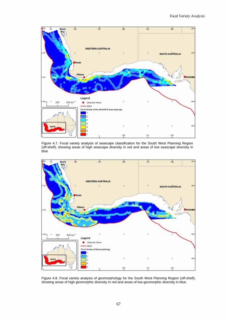
Focal Variety Analysis
67
Figure 4.7. Focal variety analysis of seascape classification for the South West Planning Region (off-shelf), showing areas of high seascape diversity in red and areas of low seascape diversity in blue
Figure 4.8. Focal variety analysis of geomorphology for the South West Planning Region (off-shelf), showing areas of high geomorphic diversity in red and areas of low geomorphic diversity in blue.
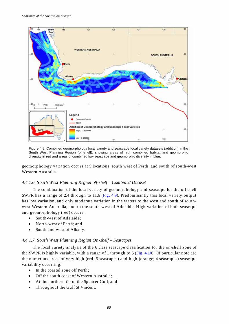
Seascapes of the Australian Margin
68
Figure 4.9. Combined geomorphology focal variety and seascape focal variety datasets (addition) in the South West Planning Region (off-shelf), showing areas of high combined habitat and geomorphic diversity in red and areas of combined low seascape and geomorphic diversity in blue.
geomorphology variation occurs at 5 locations, south west of Perth, and south of south-west Western Australia.
4.4.1.6. South West Planning Region off-shelf – Combined Dataset The combination of the focal variety of geomorphology and seascape for the off-shelf
SWPR has a range of 2.4 through to 11.6 (Fig. 4.9). Predominantly this focal variety output has low variation, and only moderate variation in the waters to the west and south of south-west Western Australia, and to the south-west of Adelaide. High variation of both seascape and geomorphology (red) occurs:
• South-west of Adelaide; • North-west of Perth; and • South and west of Albany.
4.4.1.7. South West Planning Region On-shelf – Seascapes The focal variety analysis of the 6 class seascape classification for the on-shelf zone of
the SWPR is highly variable, with a range of 1 through to 5 (Fig. 4.10). Of particular note are the numerous areas of very high (red; 5 seascapes) and high (orange; 4 seascapes) seascape variability occurring:
• In the coastal zone off Perth; • Off the south coast of Western Australia; • At the northern tip of the Spencer Gulf; and • Throughout the Gulf St Vincent.
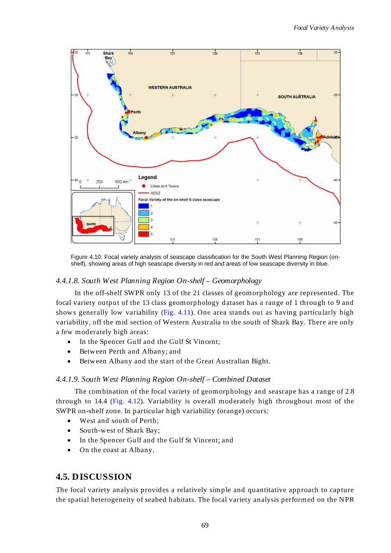
Focal Variety Analysis
69
Figure 4.10. Focal variety analysis of seascape classification for the South West Planning Region (on-shelf), showing areas of high seascape diversity in red and areas of low seascape diversity in blue.
4.4.1.8. South West Planning Region On-shelf – Geomorphology In the off-shelf SWPR only 13 of the 21 classes of geomorphology are represented. The
focal variety output of the 13 class geomorphology dataset has a range of 1 through to 9 and shows generally low variability (Fig. 4.11). One area stands out as having particularly high variability, off the mid section of Western Australia to the south of Shark Bay. There are only a few moderately high areas:
• In the Spencer Gulf and the Gulf St Vincent; • Between Perth and Albany; and • Between Albany and the start of the Great Australian Bight.
4.4.1.9. South West Planning Region On-shelf – Combined Dataset The combination of the focal variety of geomorphology and seascape has a range of 2.8
through to 14.4 (Fig. 4.12). Variability is overall moderately high throughout most of the SWPR on-shelf zone. In particular high variability (orange) occurs:
• West and south of Perth; • South-west of Shark Bay; • In the Spencer Gulf and the Gulf St Vincent; and • On the coast at Albany.
4.5. DISCUSSION The focal variety analysis provides a relatively simple and quantitative approach to capture the spatial heterogeneity of seabed habitats. The focal variety analysis performed on the NPR
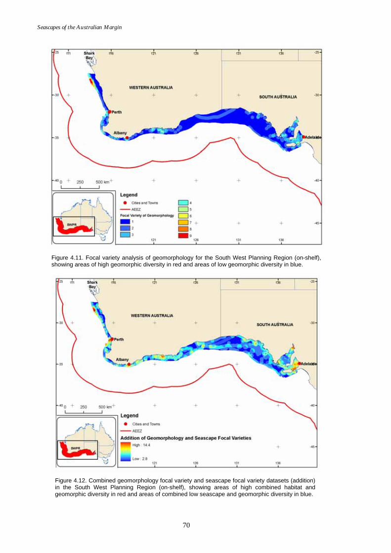
Seascapes of the Australian Margin
70
Figure 4.11. Focal variety analysis of geomorphology for the South West Planning Region (on-shelf), showing areas of high geomorphic diversity in red and areas of low geomorphic diversity in blue.
Figure 4.12. Combined geomorphology focal variety and seascape focal variety datasets (addition) in the South West Planning Region (on-shelf), showing areas of high combined habitat and geomorphic diversity in red and areas of combined low seascape and geomorphic diversity in blue.
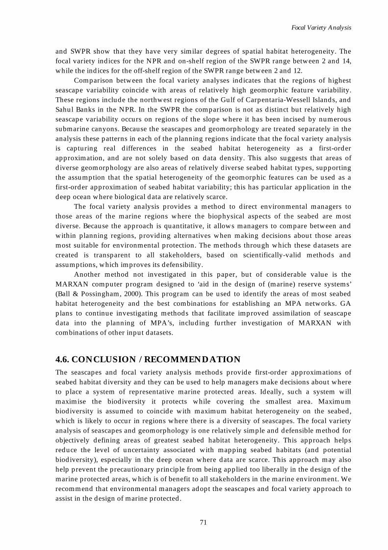
Focal Variety Analysis
71
and SWPR show that they have very similar degrees of spatial habitat heterogeneity. The focal variety indices for the NPR and on-shelf region of the SWPR range between 2 and 14, while the indices for the off-shelf region of the SWPR range between 2 and 12.
Comparison between the focal variety analyses indicates that the regions of highest seascape variability coincide with areas of relatively high geomorphic feature variability. These regions include the northwest regions of the Gulf of Carpentaria-Wessell Islands, and Sahul Banks in the NPR. In the SWPR the comparison is not as distinct but relatively high seascape variability occurs on regions of the slope where it has been incised by numerous submarine canyons. Because the seascapes and geomorphology are treated separately in the analysis these patterns in each of the planning regions indicate that the focal variety analysis is capturing real differences in the seabed habitat heterogeneity as a first-order approximation, and are not solely based on data density. This also suggests that areas of diverse geomorphology are also areas of relatively diverse seabed habitat types, supporting the assumption that the spatial heterogeneity of the geomorphic features can be used as a first-order approximation of seabed habitat variability; this has particular application in the deep ocean where biological data are relatively scarce.
The focal variety analysis provides a method to direct environmental managers to those areas of the marine regions where the biophysical aspects of the seabed are most diverse. Because the approach is quantitative, it allows managers to compare between and within planning regions, providing alternatives when making decisions about those areas most suitable for environmental protection. The methods through which these datasets are created is transparent to all stakeholders, based on scientifically-valid methods and assumptions, which improves its defensibility.
Another method not investigated in this paper, but of considerable value is the MARXAN computer program designed to ‘aid in the design of (marine) reserve systems’ (Ball & Possingham, 2000). This program can be used to identify the areas of most seabed habitat heterogeneity and the best combinations for establishing an MPA networks. GA plans to continue investigating methods that facilitate improved assimilation of seascape data into the planning of MPA’s, including further investigation of MARXAN with combinations of other input datasets.
4.6. CONCLUSION / RECOMMENDATION The seascapes and focal variety analysis methods provide first-order approximations of seabed habitat diversity and they can be used to help managers make decisions about where to place a system of representative marine protected areas. Ideally, such a system will maximise the biodiversity it protects while covering the smallest area. Maximum biodiversity is assumed to coincide with maximum habitat heterogeneity on the seabed, which is likely to occur in regions where there is a diversity of seascapes. The focal variety analysis of seascapes and geomorphology is one relatively simple and defensible method for objectively defining areas of greatest seabed habitat heterogeneity. This approach helps reduce the level of uncertainty associated with mapping seabed habitats (and potential biodiversity), especially in the deep ocean where data are scarce. This approach may also help prevent the precautionary principle from being applied too liberally in the design of the marine protected areas, which is of benefit to all stakeholders in the marine environment. We recommend that environmental managers adopt the seascapes and focal variety approach to assist in the design of marine protected.

72
PART 5 - References Auster, P.J., and Langton, R.W., 1999. The effects of fishing on fish habitat. American Fisheries
Society Symposium 22, 150-187.
Ball, I.R., and Possingham, H., 2000. MarXan V1.2 - Marine reserve design using spatially explicit annealing, a manual prepared for the Great Barrier Reef Marine Park Authority. University of Queensland, Brisbane. www.uq.edu.au.
Bax, N.J., and Williams, A., 2001. Seabed habitat on the southeast Australian continental shelf - context, vulnerability and monitoring. Marine and Freshwater Research 52, 491-512.
Beaman, R.J., and Harris, P.T., in press. Geophysical variables as predictors of megabenthos assemblages from the northern Great Barrier Reef, Australia. In: Todd, B.J., Greene, H.G., (Eds), Mapping the Seafloor for Habitat Characterization. Geological Association of Canada, Special Paper.
Bezdek, J.C., 1974. Cluster validity with fuzzy sets. Journal of Cybernetics 3, 58-73.
Bezdek, J.C., 1992. Computing with uncertainty. IEEE Communications Magazine 1, 24-36.
Bezdek, J.C., Erhlich, R., and Full, W., 1984. FCM: The fuzzy c-means clustering algorithm. Computers and Geosciences 10, 191-203.
Burrough, P.A., van Gaans, P.F.M, and Hootsmans, R.J., 1997. Continuous classification in soil survey: Spatial correlation, confusion and boundaries. Geoderma 77,115-135.
Burrough, P.A., and McDonnell, R.A., 1998. Principles of Geographic Information Systems. Oxford University Press, USA.
Burrough, P.A., van Gaans, P., and MacMillan, R., 2000. High-resolution landform classification using fuzzy k-means. Fuzzy Sets and Systems 113, 37-52.
Calinski, T., and Harabasz, J., 1974. A dendrite method for cluster analysis. Communications in Statistics 3, 1-27.
Connell, J.H. 1978. Diversity in Tropical Rain Forests and Coral Reefs. Science 199, 1302-1310.
Connell Wagner, 2000. NRSMPA Strategic Plan of Action: Status of Ecosystem Mapping for NRSMPA, Report on Action 6. Environment Australia, Canberra.
Davies, D.L., and Bouldin, D.W., 1979. A cluster separation measure. IEEE Transactions on Pattern Analysis and Machine Intelligence 1, 224-227.
Day, J.C. and Roff, J.C., 2000. Planning for Representative Marine Protected Areas: A Framework for Canada’s Oceans. WWF Canada, Toronto. 147pp.
de Fontaubert, A.C., Downes, D.R., and Agardy, T.S., 1996. Biodiversity in the Seas: Implementing the Convention on Biological Diversity in Marine and Coastal Habitats. IUCN, Gland.
de Forges, G.R., Koslow, J.A., and Poore, G.C.B., 2000. Diversity and endemism of the benthic seamount fauna in the southwest Pacific. Nature 405, 944-947.
Department of the Environment and Heritage, 2005. National Marine Bioregionalisation of Australia 2005. DVD and Summary booklet. Commonwealth of Australia, Canberra.
References
73
Dunn, J.C., 1973. A fuzzy relative of the isodata process and its use in detecting compact well separated clusters. Journal of Cybernetics 28, 32-57.
Earth Resources Mapping Ltd. (ER Mapper), 2007. ER Mapper v 7.1 User Guide, USA.
Environmental Systems Research Institute, Inc. (ESRI), 2006. ArcGIS v9.1 Online Help Menu, California, USA.
Etter, R.J., and Grassle, J.F., 1992. Patterns of species diversity in the deep sea as a function of sediment particle size diversity. Nature 360, 576-578.
Folk, R.L., 1966. A review of grain-size parameters. Sedimentology 6, 79-93.
Fonseca, M.S., and Bell, S.S., 1998. Influence of physical setting on seagrass landscapes near Neaufort, North Carolina, USA. Marine Ecology Progress Series 171, 109-121.
Gath, I. and Geva, A.B., 1989. Unsupervised optimal fuzzy clustering. IEEE Transactions of Pattern Analysis and Machine Intelligence 11, 773-781.
Golding, N., Vincent, M.A., and Connor, D.W., 2004. Irish Sea Pilot - Report on the development of a marine landscape classification for the Irish Sea 346. Joint Nature Conservation Committee, Peterborough, U.K. www.jncc.gov.uk/irishseapilot.
Greene, H.G., Yoklavich, M.M., Sullivan, D., and Cailliet, G.M., 1995. A geophysical approach to classifying marine benthic habitats: Monterey Bay as a model. In: O'Connell, T., and Wakefield, W., (Eds), Applications of side-scan sonar and laser-line systems in fisheries research. Alaska Fish and Game Species Publication 9. p. 15-30.
Harris, P.T., Heap, A.D., Passlow, V., Hughes, M., Daniell, J., Hemer, M., and Anderson, O., 2005. Tidally incised valleys on tropical carbonate shelves: An example from the northern Great Barrier Reef, Australia. Marine Geology 220, 181-204.
Harris, P.T., Heap, A.D., Wassenberg, T., and Passlow, V., 2004. Submerged coral reefs in the Gulf of Carpentaria, Australia. Marine Geology 207, 185-191.
Harris, P., Heap, A., Passlow, V., Sbaffi, L., Fellows, M., Porter-Smith, R., Buchanan, C., and Daniell, J., 2003. Geomorphic Features of the Continental Margin of Australia. Geoscience Australia, Record 2003/30. Geoscience Australia, Canberra. 141pp.
Hemer, M.A., 2006. The magnitude and frequency of combined flow bed shear stress as a measure of exposure on the Australian continental shelf. Continental Shelf Research 26, 1258-1280.
Hill, B.J., Haywood, M., Venables, B., Gordon, S.R., Condie, S., Ellis, N.R., Tyre, A., Vance, D., Dunn, J., Mansbridge, J., Moeseneder, C., Bustamante, R., and Pantus, F., 2002. Surrogates I - Predictors, impacts, management and conservation of the benthic biodiversity of the Northern Prawn Fishery. Final Report on FRDC Project 2000/160. CSIRO, Cleveland.
Hinde A., Ruddick, R., Whiteway, T., and Heap, A.D., 2007. Seascapes of the Australian Margin and Adjacent Sea Floor: Keystroke Methodology. Geoscience Australia, Record 2007/10. Geoscience Australia, Canberra. 56pp.
IMCRA Technical Group, 1998. Interim Marine and Coastal Regionalisation for Australia: An ecosystem-based classification for marine and coastal environments. Version 3.3. Environment Australia, Canberra. 104pp.
Seascapes of the Australian Margin
74
James, N.P., Bone, Y., Collins, L.B., and Kyser, T.K., 2001. Surficial sediments of the Great Australian Bight: Facies dynamics and oceanography of a vast cool-water carbonate shelf. Journal of Sedimentary Research, Section B: Stratigraphy and Global Studies 71, 549-567.
James, N.P., Collins, L.B., Bone, Y., and Hallock, P., 1999. Subtropical carbonates in a temperate realm: Modern sediments on the southwest Australian shelf. Journal of Sedimentary Research 69, 1297-1321.
James, N.P., Bone, Y., Hageman, S.J., Feary, D.A., and Gostin, V.A., 1997. Cool-water carbonate sedimentation during the terminal Quaternary sea-level cycle: Lincoln Shelf, southern Australia. In: James, N.P. and Clarke, J.A.D., (Eds), Cool-water Carbonates. SEPM (Society for Sedimentary Geology) Special Publication 56, pp.53-75.
Jongsma, D., 1974. Marine Geology of the Arafura Sea. Bureau of Mineral Resources Bulletin, 157. 73pp.
Kostylev, V.E., Todd, B.J., Fader, G.B.J., Courtney, R.C., Cameron, G.D.M., and Pickrill, R.A., 2001. Benthic habitat mapping on the Scotian Shelf based on multibeam bathymetry, surficial geology and sea floor photographs. Marine Ecology Progress Series 219, 121-137.
Logan, G.A., Rollet, N., Glenn, K., Grosjean, E., Ryan, G.J., and Shipboard Party, 2006. Shallow Gas and Benthic Habitat Mapping, Arafura Sea. Geoscience Australia, Record 2006/19. 338pp.
Long, B.G. and Poiner, I.R., 1994. Infaunal benthic community structure and function in the Gulf of Carpentaria, Northern Australia. Australian Journal of Marine and Freshwater Research 45, 293-316.
Long, B.G., Poiner, I.R., and Wassenberg, T.J., 1995. Distribution, biomass and community structure of megabenthos of the Gulf of Carpentaria, Australia. Marine Ecology Progress Series 129, 127-139.
Orpin, A. R., and Kostylev, V. E., 2006, Towards a statistically valid method of textural sea floor characterization of benthic habitats. Marine Geology 225, 209-222.
Pakhira, M.K., Bandyopadhyay, S., and Maulik, U., 2005. A study of some fuzzy cluster validity indices, genetic clustering and application to pixel classification. Fuzzy Sets and Systems 155, 191-214.
Pal, N.R. and Bezdek, J.C., 1995. On cluster validity for the fuzzy c-means model. IEEE Transactions of Fuzzy Systems 3, 370-379.
Passlow, T., Rogis, J., Hancock, A., Hemer, M., Kriton, G., Habib, A., 2005. National Marine Sediments Database and Seafloor Characteristics Project. Geoscience Australia, Record 2005/08. Geoscience Australia, Canberra. 110pp.
Pitcher, R., Venables, B., Pantus, F., Ellis, N., McLeod, I., Austin, M., Gribble, N., and Doherty, P., 2002. GBR Seabed Biodiversity Mapping Project: Phase 1. Draft Report to CRC-Reef. CSIRO Marine Research, Cleveland.
Post, A.L., Wassenburg, T., and Passlow, V. 2006. Physical surrogates for macrofaunal distributions and abundance in a tropical gulf. Marine and Freshwater Research 57, 469-483.
References
75
Potter, A., Southby, C., and Heap, A.D., in press. Sedimentology and Geomorphology of the South West Planning Region of Australia. Geoscience Australia, Record. Geoscience Australia, Canberra.
Ramey, P.A., and Snelgrove, P.V.R., 2003. Spatial patterns in sedimentary macrofaunal communities on the south coast of Newfoundland in relation to surface oceanography and sediment characteristics. Marine Ecology Progress Series 262, 215-227
Rochester, W.A., Milton, D.A., Moeseneder, C.H., Miller, M.J., Fry, G.C., Pillans, R.D., Bustamante, R.H., Butler, A.J., 2007. The North Marine Region Marine Bioregional Plan: Information and Analysis for the Regional Profile. Final report to the Department of the Environment and Heritage. CSIRO, Cleveland.
Roff, J.C., and Taylor, M.E., 2000. National frameworks for marine conservation - a hierarchical geophysical approach. Aquatic Conservation: Marine and Freshwater Ecosystems 10, 209-223.
Roff, J.C., Taylor, M.E., and Laughren, J., 2003. Geophysical approaches to the classification, delineation and monitoring of marine habitats and their communities. Aquatic Conservation: Marine and Freshwater Ecosystems 13, 77-90.
Snelgrove, P.V.R., and Butman, C.A., 1994. Animal sediment relationships revisited: cause versus effect. Oceanography and Marine Biology: An Annual Review 32, 111-127.
Somers, I.F., 1994. Species composition and distribution of commercial penaeid prawn catches in the Gulf of Carpentaria, Australia, in relation to depth and sediment type. Australian Journal of Marine and Freshwater Research 45, 317-335.
Thouzeau, G., Robert, G., and Ugarte, R., 1991. Faunal assemblages of benthic megainvertebrates inhabiting sea scallop grounds from eastern Georges Bank, in relation to environmental factors. Marine Ecology Progress Series 74, 61-82.
Todd, B.J., Fader, G.B.J., Courtney, R.C., and Pickrill, R.A., 1999. Quaternary geology and surficial sediment processes, Browns Bank, Scotian Shelf, based on multibeam bathymetry. Marine Geology 162, 165-214.
Vetter, E.W. and Dayton, P.K., 1998. Macrofaunal communities within and adjacent to a detritus-rich submarine canyon system. Deep-Sea Research II 45, 25-54.
Warwick, R.M., and Uncles, R.J., 1980. Distribution of benthic macrofaunal associations in the Bristol Channel in relation to tidal stress. Marine Ecology Progress Series 3, 97-103.
Webster, M., and Petkovic, P., 2005. Australian Bathymetry and Topography Grid. GA Record 2005/12. Geoscience Australia, Canberra. 2x DVD.
Wu, K.L., and Yang, M., 2005. Alternative c-means clustering algorithms. Pattern Recognition 35, 2267-2278.
Xie, X.L., and Beni, G., 1991. A validity measure for fuzzy clustering. IEEE Transactions on Pattern Analysis 13, 841-847.
Zadeh, L.A., 1965. Fuzzy Sets. Information Control 8, 338-353.
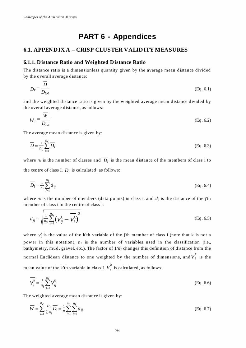
Seascapes of the Australian Margin
76
PART 6 - Appendices
6.1. APPENDIX A – CRISP CLUSTER VALIDITY MEASURES
6.1.1. Distance Ratio and Weighted Distance Ratio The distance ratio is a dimensionless quantity given by the average mean distance divided by the overall average distance:
DD
Dtot
r = (Eq. 6.1)
and the weighted distance ratio is given by the weighted average mean distance divided by the overall average distance, as follows:
DW
Wtot
r = (Eq. 6.2)
The average mean distance is given by:
∑=
=n
ic
c
iDD n
1
1 (Eq. 6.3)
where nc is the number of classes and Di is the mean distance of the members of class i to
the centre of class I. Di is calculated, as follows:
∑=
=ni
iji
ij
dD n1
1 (Eq. 6.4)
where ni is the number of members (data points) in class i, and dij is the distance of the j'th member of class i to the centre of class i:
∑ −=
=n
ki
kijvij
v
kvvnd
1)(
21 (Eq. 6.5)
where vkij is the value of the k'th variable of the j'th member of class i (note that k is not a
power in this notation), nv is the number of variables used in the classification (i.e., bathymetry, mud, gravel, etc.). The factor of 1/nv changes this definition of distance from the
normal Euclidean distance to one weighted by the number of dimensions, andVki is the
mean value of the k'th variable in class I. Vki is calculated, as follows:
∑=
=ni k
iji
ki
jvv n
1
1 (Eq. 6.6)
The weighted average mean distance is given by:
∑∑∑= ==
==∑
nc niijni
nc
nii
i ji
dDnW1 11
1 (Eq. 6.7)

Appendices
77
where n = Σni is the total number of data points in all classes. The overall average distance is given by:
∑∑ ∑= = =
−=n n n
kkijv
totc
i
i
j
v
kVVD nn
1 1 1
2)(11 (Eq. 6.8)
where Vk is the mean value of the k'th variable and calculated as follows:
∑∑==
=nn ic
j
k
iji
ic
kVV nn
11
11 (Eq. 6.9)
6.1.2. Calinski-Harabasz Pseudo F-statistic The Calinski-Harabasz pseudo F-statistic is defined as:
⎟⎠
⎞⎜⎝
⎛−−
⎟⎠
⎞⎜⎝
⎛−
=
nnR
nR
F
c
cCH 1
12
2
(Eq. 6.10)
where n = Σni is the total number of data points in all classes, nc is the number of classes, and
SSTSSESST
R−
=2 (Eq. 6.11)
where SST is the total sum of squared distances to the overall mean (similar to the between-groups sum of squares). SST is calculated, as follows:
∑∑∑ −= = =
=n n n
VVSSTc
i
i
j
v
k
kkij
1 1 1
2)( (Eq. 6.12)
and SSE is the sum of squared distances of the data points to their own class means (similar to the within group sum of squares). SSE is calculated, as follows:
∑∑∑ −= = =
=n n n
VVSSEc
i
i
j
v
k
ki
kij
1 1 1
2)( (Eq. 6.12)
where ni is the number of members (data points) in class i, nv is the number of variables used
in the classification (bathymetry, mud, gravel, etc.), vkij is the value of the k'th variable of the
j'th member of class i (note that k is not a power in this notation), Vk is the mean value of the
k'th variable, and Vki is the mean over all observations of the k'th variable in class i. For
computational purposes, FCH is more conveniently written as:
⎟⎟⎠
⎞⎜⎜⎝
⎛−−
⎟⎠⎞
⎜⎝⎛ −=
11
nnn
SSESST
Fc
cCH
(Eq. 6.13)
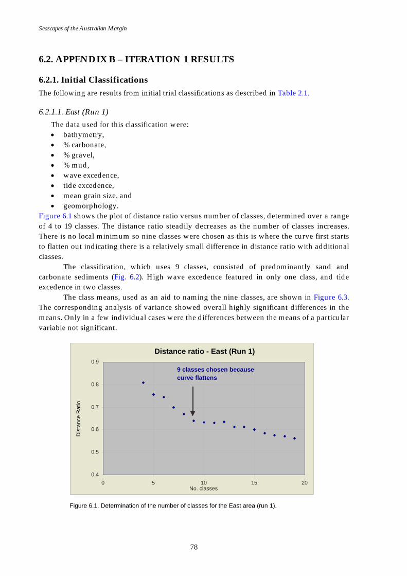
Seascapes of the Australian Margin
78
6.2. APPENDIX B – ITERATION 1 RESULTS
6.2.1. Initial Classifications The following are results from initial trial classifications as described in Table 2.1.
6.2.1.1. East (Run 1) The data used for this classification were: • bathymetry, • % carbonate, • % gravel, • % mud, • wave excedence, • tide excedence, • mean grain size, and • geomorphology.
Figure 6.1 shows the plot of distance ratio versus number of classes, determined over a range of 4 to 19 classes. The distance ratio steadily decreases as the number of classes increases. There is no local minimum so nine classes were chosen as this is where the curve first starts to flatten out indicating there is a relatively small difference in distance ratio with additional classes.
The classification, which uses 9 classes, consisted of predominantly sand and carbonate sediments (Fig. 6.2). High wave excedence featured in only one class, and tide excedence in two classes.
The class means, used as an aid to naming the nine classes, are shown in Figure 6.3. The corresponding analysis of variance showed overall highly significant differences in the means. Only in a few individual cases were the differences between the means of a particular variable not significant.
Figure 6.1. Determination of the number of classes for the East area (run 1).
Distance ratio - East (Run 1)
0.4
0.5
0.6
0.7
0.8
0.9
0 5 10 15 20 No. classes
9 classes chosen because curve flattens
Dis
tanc
e R
atio
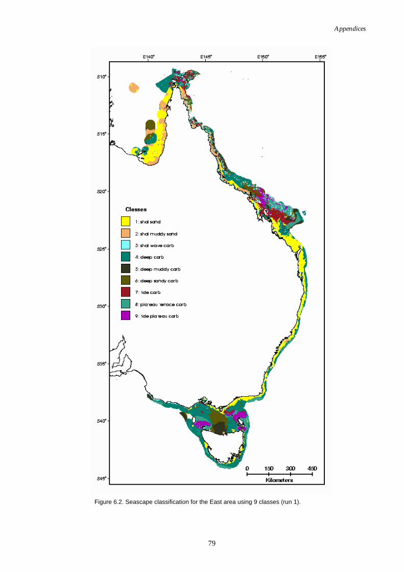
Appendices
79
Figure 6.2. Seascape classification for the East area using 9 classes (run 1).
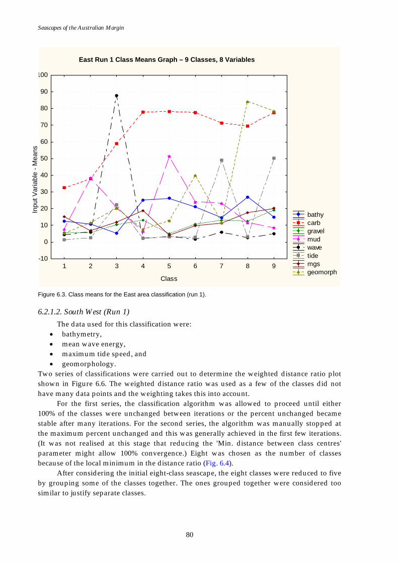
Seascapes of the Australian Margin
80
East - 9 classes - LS meansWilks lambda=.00126, F(64, 3188E3)=1086E2, p=0.0000
bathy carb gravel mud wave tide mgs geomorph
1 2 3 4 5 6 7 8 9
Class
-10
0
10
20
30
40
50
60
70
80
90
100
Figure 6.3. Class means for the East area classification (run 1).
6.2.1.2. South West (Run 1) The data used for this classification were:
• bathymetry, • mean wave energy, • maximum tide speed, and • geomorphology.
Two series of classifications were carried out to determine the weighted distance ratio plot shown in Figure 6.6. The weighted distance ratio was used as a few of the classes did not have many data points and the weighting takes this into account.
For the first series, the classification algorithm was allowed to proceed until either 100% of the classes were unchanged between iterations or the percent unchanged became stable after many iterations. For the second series, the algorithm was manually stopped at the maximum percent unchanged and this was generally achieved in the first few iterations. (It was not realised at this stage that reducing the 'Min. distance between class centres' parameter might allow 100% convergence.) Eight was chosen as the number of classes because of the local minimum in the distance ratio (Fig. 6.4).
After considering the initial eight-class seascape, the eight classes were reduced to five by grouping some of the classes together. The ones grouped together were considered too similar to justify separate classes.
Inpu
t Var
iabl
e - M
eans
East Run 1 Class Means Graph – 9 Classes, 8 Variables
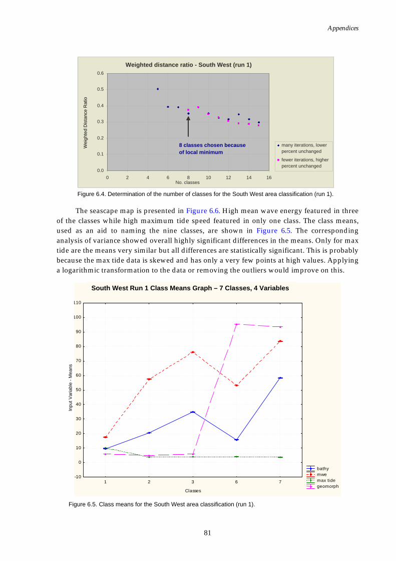
Appendices
81
Figure 6.4. Determination of the number of classes for the South West area classification (run 1).
The seascape map is presented in Figure 6.6. High mean wave energy featured in three of the classes while high maximum tide speed featured in only one class. The class means, used as an aid to naming the nine classes, are shown in Figure 6.5. The corresponding analysis of variance showed overall highly significant differences in the means. Only for max tide are the means very similar but all differences are statistically significant. This is probably because the max tide data is skewed and has only a very few points at high values. Applying a logarithmic transformation to the data or removing the outliers would improve on this.
South West - 5 classes from 8 classes - LS MeansWilks lambda=.00231, F(16, 8381E2)=3297E2, p=0.0000
bathy mwe max tide geomorph
1 2 3 6 7
Classes
-10
0
10
20
30
40
50
60
70
80
90
100
110
Figure 6.5. Class means for the South West area classification (run 1).
Weighted distance ratio - South West (run 1)
0.0
0.1
0.2
0.3
0.4
0.5
0.6
0 2 4 6 8 10 12 14 16No. classes
many iterations, lower percent unchanged fewer iterations, higherpercent unchanged
8 classes chosen because of local minimum
Wei
ghte
d D
ista
nce
Rat
io
Inpu
t Var
iabl
e - M
eans
South West Run 1 Class Means Graph – 7 Classes, 4 Variables
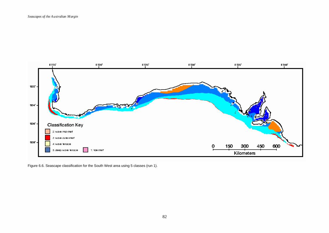
Seascapes of the Australian Margin
82
Figure 6.6. Seascape classification for the South West area using 5 classes (run 1).
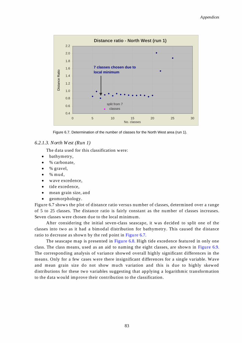
Appendices
83
Figure 6.7. Determination of the number of classes for the North West area (run 1).
6.2.1.3. North West (Run 1) The data used for this classification were:
• bathymetry, • % carbonate, • % gravel, • % mud, • wave excedence, • tide excedence, • mean grain size, and • geomorphology.
Figure 6.7 shows the plot of distance ratio versus number of classes, determined over a range of 5 to 25 classes. The distance ratio is fairly constant as the number of classes increases. Seven classes were chosen due to the local minimum.
After considering the initial seven-class seascape, it was decided to split one of the classes into two as it had a bimodal distribution for bathymetry. This caused the distance ratio to decrease as shown by the red point in Figure 6.7.
The seascape map is presented in Figure 6.8. High tide excedence featured in only one class. The class means, used as an aid to naming the eight classes, are shown in Figure 6.9. The corresponding analysis of variance showed overall highly significant differences in the means. Only for a few cases were there insignificant differences for a single variable. Wave and mean grain size do not show much variation and this is due to highly skewed distributions for these two variables suggesting that applying a logarithmic transformation to the data would improve their contribution to the classification.
Distance ratio - North West (run 1)
split from 7 classes
0.4 0.6
0.8 1.0 1.2
1.4 1.6 1.8
2.0 2.2
0 5 10 15 20 25 30 No. classes
7 classes chosen due to local minimum
Dis
tanc
e R
atio
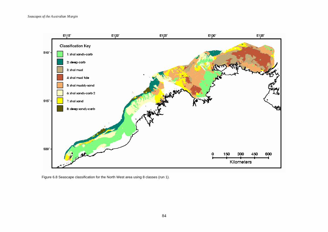
Seascapes of the Australian Margin
84
Figure 6.8 Seascape classification for the North West area using 8 classes (run 1).
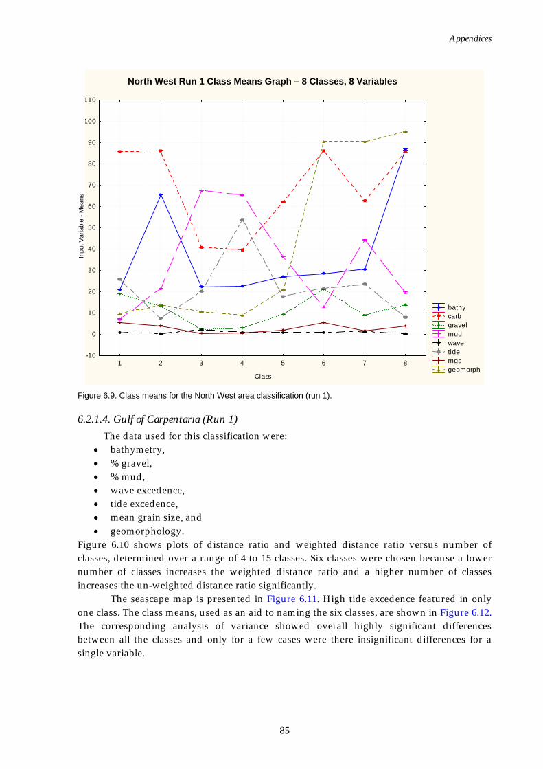
Appendices
85
North West - 8 classes (7 split) - LS MeansWilks lambda=.00441, F(56, 2681E3)=83179., p=0.0000
bathy carb gravel mud wave tide mgs geomorph
1 2 3 4 5 6 7 8
Class
-10
0
10
20
30
40
50
60
70
80
90
100
110
Figure 6.9. Class means for the North West area classification (run 1).
6.2.1.4. Gulf of Carpentaria (Run 1) The data used for this classification were:
• bathymetry, • % gravel, • % mud, • wave excedence, • tide excedence, • mean grain size, and • geomorphology.
Figure 6.10 shows plots of distance ratio and weighted distance ratio versus number of classes, determined over a range of 4 to 15 classes. Six classes were chosen because a lower number of classes increases the weighted distance ratio and a higher number of classes increases the un-weighted distance ratio significantly.
The seascape map is presented in Figure 6.11. High tide excedence featured in only one class. The class means, used as an aid to naming the six classes, are shown in Figure 6.12. The corresponding analysis of variance showed overall highly significant differences between all the classes and only for a few cases were there insignificant differences for a single variable.
Inpu
t Var
iabl
e - M
eans
North West Run 1 Class Means Graph – 8 Classes, 8 Variables
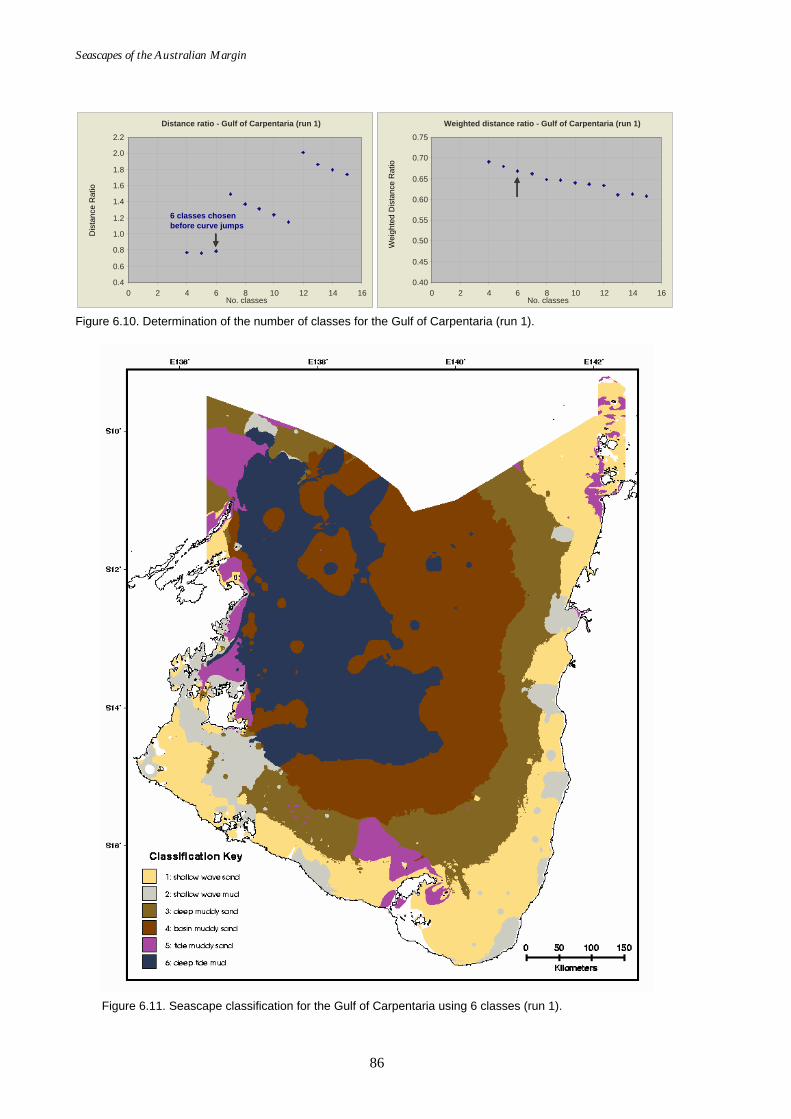
Seascapes of the Australian Margin
86
Figure 6.10. Determination of the number of classes for the Gulf of Carpentaria (run 1).
Figure 6.11. Seascape classification for the Gulf of Carpentaria using 6 classes (run 1).
Distance ratio - Gulf of Carpentaria (run 1)
0.4 0.6 0.8 1.0 1.2 1.4 1.6 1.8 2.0 2.2
0 2 4 6 8 10 12 14 16No. classes
6 classes chosen before curve jumps
Dis
tanc
e R
atio
Weighted distance ratio - Gulf of Carpentaria (run 1)
0.40
0.45
0.50
0.55
0.60
0.65
0.70
0.75
0 2 4 6 8 10 12 14 16No. classes
Wei
ghte
d D
ista
nce
Rat
io
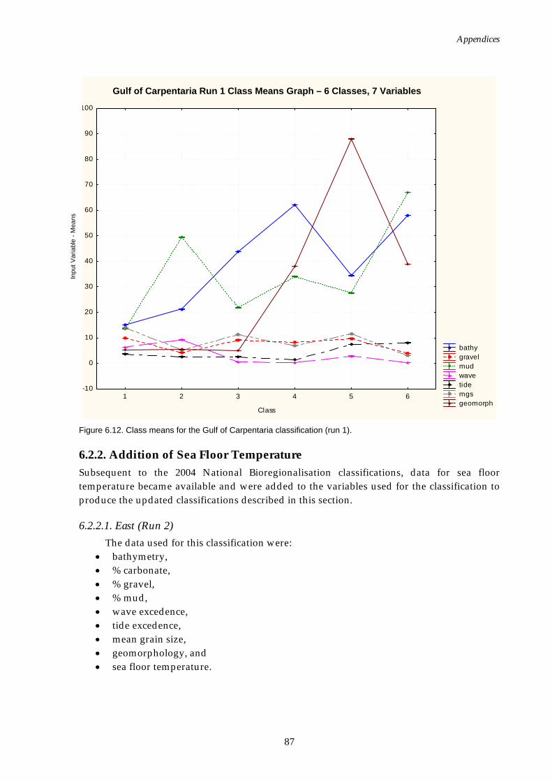
Appendices
87
Gulf of Carpentaria - 6 classes - LS MeansWilks lambda=.00511, F(35, 1464E3)=1048E2, p=0.0000
bathy gravel mud wave tide mgs geomorph
1 2 3 4 5 6
Class
-10
0
10
20
30
40
50
60
70
80
90
100
Figure 6.12. Class means for the Gulf of Carpentaria classification (run 1).
6.2.2. Addition of Sea Floor Temperature Subsequent to the 2004 National Bioregionalisation classifications, data for sea floor temperature became available and were added to the variables used for the classification to produce the updated classifications described in this section.
6.2.2.1. East (Run 2) The data used for this classification were:
• bathymetry, • % carbonate, • % gravel, • % mud, • wave excedence, • tide excedence, • mean grain size, • geomorphology, and • sea floor temperature.
Inpu
t Var
iabl
e - M
eans
Gulf of Carpentaria Run 1 Class Means Graph – 6 Classes, 7 Variables
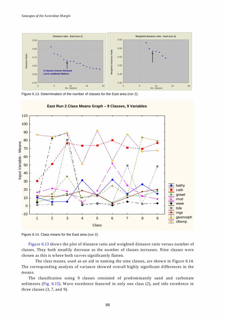
Seascapes of the Australian Margin
88
Figure 6.13. Determination of the number of classes for the East area (run 2).
East sft - 9 classes - LS meansWilks lambda=.00056, F(72, 3362E3)=1134E2, p=0.0000
bathy carb gravel mud wave tide mgs geomorph sftemp
1 2 3 4 5 6 7 8 9
Class
-10
0
10
20
30
40
50
60
70
80
90
100
110
Figure 6.14. Class means for the East area (run 2).
Figure 6.13 shows the plot of distance ratio and weighted distance ratio versus number of classes. They both steadily decrease as the number of classes increases. Nine classes were chosen as this is where both curves significantly flatten.
The class means, used as an aid to naming the nine classes, are shown in Figure 6.14. The corresponding analysis of variance showed overall highly significant differences in the means.
The classification using 9 classes consisted of predominantly sand and carbonate sediments (Fig. 6.15). Wave excedence featured in only one class (2), and tide excedence in three classes (3, 7, and 9).
Distance ratio - East (run 2)
0.40
0.50
0.60
0.70
0.80
0.90
0 5 10 15 20No. classes
9 classes chosen because curve suddenly flattens
Dis
tanc
e R
atio
Weighted distance ratio - East (run 2)
0.40
0.45
0.50
0.55
0.60
0.65
0 5 10 15 20No. classes
Wei
ghte
d D
ista
nce
Rat
io
Inpu
t Var
iabl
e - M
eans
East Run 2 Class Means Graph – 9 Classes, 9 Variables

Appendices
89
Figure 6.15. Seascape classification for East area using 9 classes (run 2).
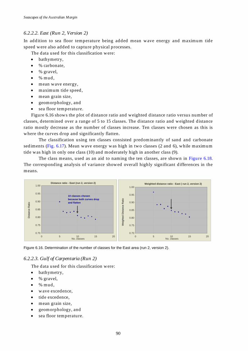
Seascapes of the Australian Margin
90
6.2.2.2. East (Run 2, Version 2) In addition to sea floor temperature being added mean wave energy and maximum tide speed were also added to capture physical processes.
The data used for this classification were: • bathymetry, • % carbonate, • % gravel, • % mud, • mean wave energy, • maximum tide speed, • mean grain size, • geomorphology, and • sea floor temperature. Figure 6.16 shows the plot of distance ratio and weighted distance ratio versus number of
classes, determined over a range of 5 to 15 classes. The distance ratio and weighted distance ratio mostly decrease as the number of classes increase. Ten classes were chosen as this is where the curves drop and significantly flatten.
The classification using ten classes consisted predominantly of sand and carbonate sediments (Fig. 6.17). Mean wave energy was high in two classes (2 and 6), while maximum tide was high in only one class (10) and moderately high in another class (9).
The class means, used as an aid to naming the ten classes, are shown in Figure 6.18. The corresponding analysis of variance showed overall highly significant differences in the means.
Figure 6.16. Determination of the number of classes for the East area (run 2, version 2).
6.2.2.3. Gulf of Carpentaria (Run 2) The data used for this classification were: • bathymetry, • % gravel, • % mud, • wave excedence, • tide excedence, • mean grain size, • geomorphology, and • sea floor temperature.
Distance ratio - East (run 2, version 2)
0.70
0.75
0.80
0.85
0.90
0.95
1.00
0 5 10 15 20No. classes
10 classes chosen because both curves drop and flatten
Dis
tanc
e R
atio
Weighted distance ratio - East ( run 2, version 2)
0.70
0.75
0.80
0.85
0.90
0.95
1.00
0 5 10 15 20No. classes
Wei
ghte
d D
ista
nce
Rat
io
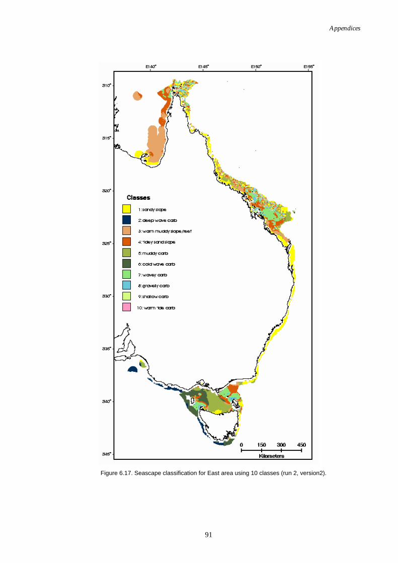
Appendices
91
Figure 6.17. Seascape classification for East area using 10 classes (run 2, version2).

Seascapes of the Australian Margin
92
East (mwe & max tide) + sf temp - 10 classes - LS MeansWilks lambda=.00832, F(81, 2781E3)=37700., p=0.0000
bathy carb gravel mud mwe max tide mgs geomorph sf temp
1 2 3 4 5 6 7 8 9 10
Class
-10
0
10
20
30
40
50
60
70
80
90
100
110
Figure 6.18. Class means for the East area (run 2, version 2).
Figure 6.19. Determination of the number of classes for the Gulf of Carpentaria (run 2).
Figure 6.19 shows plots of distance ratio and weighted distance ratio versus number of classes, determined over a range of 5 to 15 classes. The weighted distance ratio curve steadily decreases with a notable flattening at 6 classes, whereas the unweighted distance ratio is more erratic with a minimum at 11 classes. The weighted curve justifies fewer classes (6) due to its flattening.
The classification consisted mainly of muds and sands with one gravel class (Fig. 6.20). Tide excedence was high in two classes (2 and 5) while wave excedence was rather low in all classes. The distributions for both these variables are highly skewed indicating that it would be better to use logarithms.
The class means, used as an aid to naming the six classes, are shown in Figure 6.21. The corresponding analysis of variance showed overall highly significant differences in the means. Only for a few cases were there insignificant differences for a single variable.
Distance ratio - Gulf of Carpentaria (run 2)
0.80
0.90
1.00
1.10
1.20
1.30
0 2 4 6 8 10 12 14 16No. classes
Dis
tanc
e R
atio
Weighted distance ratio - Gulf of Carpentaria (run 2)
0.70
0.75
0.80
0.85
0.90
0.95
1.00
0 2 4 6 8 10 12 14 16No. classes
6 classes chosen because curve flattens W
eigh
ted
Dis
tanc
e R
atio
Inpu
t Var
iabl
e - M
eans
East Run 2, version 2 Class Means Graph – 10 Classes, 9 Variables
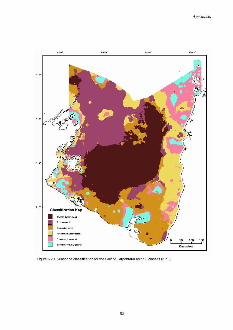
Appendices
93
Figure 6.20. Seascape classification for the Gulf of Carpentaria using 6 classes (run 2).
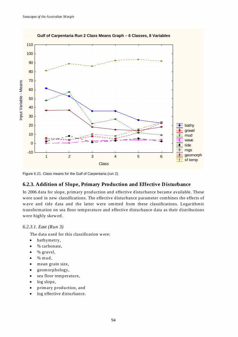
Seascapes of the Australian Margin
94
Gulf of Carpentaria + sft - LS MeansWilks lambda=.02556, F(40, 1490E3)=49142., p=0.0000
bathy gravel mud wave tide mgs geomorph sf temp
1 2 3 4 5 6
Class
-10
0
10
20
30
40
50
60
70
80
90
100
110
Figure 6.21. Class means for the Gulf of Carpentaria (run 2).
6.2.3. Addition of Slope, Primary Production and Effective Disturbance In 2006 data for slope, primary production and effective disturbance became available. These were used in new classifications. The effective disturbance parameter combines the effects of wave and tide data and the latter were omitted from these classifications. Logarithmic transformation on sea floor temperature and effective disturbance data as their distributions were highly skewed.
6.2.3.1. East (Run 3) The data used for this classification were: • bathymetry, • % carbonate, • % gravel, • % mud, • mean grain size, • geomorphology, • sea floor temperature, • log slope, • primary production, and • log effective disturbance.
Inpu
t Var
iabl
e - M
eans
Gulf of Carpentaria Run 2 Class Means Graph – 6 Classes, 8 Variables
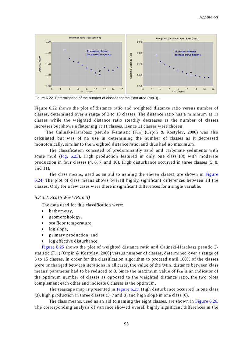
Appendices
95
Figure 6.22. Determination of the number of classes for the East area (run 3).
Figure 6.22 shows the plot of distance ratio and weighted distance ratio versus number of classes, determined over a range of 3 to 15 classes. The distance ratio has a minimum at 11 classes while the weighted distance ratio steadily decreases as the number of classes increases but shows a flattening at 11 classes. Hence 11 classes were chosen.
The Calinski-Harabasz pseudo F-statistic (FCH) (Orpin & Kostylev, 2006) was also calculated but was of no use in determining the number of classes as it decreased monotonically, similar to the weighted distance ratio, and thus had no maximum.
The classification consisted of predominantly sand and carbonate sediments with some mud (Fig. 6.23). High production featured in only one class (3), with moderate production in four classes (4, 6, 7, and 10). High disturbance occurred in three classes (5, 8, and 11).
The class means, used as an aid to naming the eleven classes, are shown in Figure 6.24. The plot of class means shows overall highly significant differences between all the classes. Only for a few cases were there insignificant differences for a single variable.
6.2.3.2. South West (Run 3) The data used for this classification were: • bathymetry, • geomorphology, • sea floor temperature, • log slope, • primary production, and • log effective disturbance. Figure 6.25 shows the plot of weighted distance ratio and Calinski-Harabasz pseudo F-
statistic (FCH) (Orpin & Kostylev, 2006) versus number of classes, determined over a range of 3 to 15 classes. In order for the classification algorithm to proceed until 100% of the classes were unchanged between iterations in all cases, the value of the 'Min. distance between class means' parameter had to be reduced to 3. Since the maximum value of FCH is an indicator of the optimum number of classes as opposed to the weighted distance ratio, the two plots complement each other and indicate 8 classes is the optimum.
The seascape map is presented in Figure 6.25. High disturbance occurred in one class (3), high production in three classes (3, 7 and 8) and high slope in one class (6).
The class means, used as an aid to naming the eight classes, are shown in Figure 6.26. The corresponding analysis of variance showed overall highly significant differences in the
Distance ratio - East (run 3)
0.50
0.60
0.70
0.80
0.90
0 2 4 6 8 10 12 14 16No. classes
11 classes chosen because curve jumps
Dis
tanc
e R
atio
Weighted Distance ratio - East (run 3)
0.50
0.60
0.70
0.80
0.90
0 2 4 6 8 10 12 14 16No. classes
11 classes chosen because curve flattens
Wei
ghte
d D
ista
nce
Rat
io
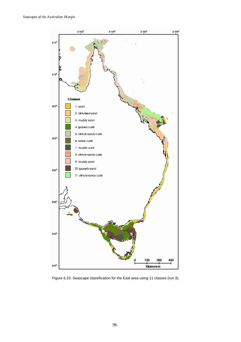
Seascapes of the Australian Margin
96
Figure 6.23. Seascape classification for the East area using 11 classes (run 3).

Appendices
97
East (effective disturbance) 10 vars; Class; LS MeansWilks lambda=.00034, F(100, 3540E3)=72535., p=0.0000
bathymetry carbonate gravel mud mean grain size geomorph sea floor temp ln slope 5000 primary prodn log effective disturbance
1 2 3 4 5 6 7 8 9 10 11
Class
-10
0
10
20
30
40
50
60
70
80
90
100
Figure 6.24. Class means for the East area (run 3).
Figure 6.25. Determination of the number of classes for South West area (run 3).
means. The only means with no statistical difference are between classes 1 and 6 for log effective disturbance. Note that the geomorphology for classes 1 to 4 are very similar, being mostly shelf, and those for classes 5 to 8 are also similar being mostly terrace.
Weighted distance ratio - South West (run 3)
0.95
0.96
0.97
0.98
0.99
1.00
0 2 4 6 8 10 12 14 16No. classes
8 classes chosen because of minimum
Wei
ghte
d D
ista
nce
Rat
io
CH F-statistic - South West (run 3)
0
200
400
600
800
1000
0 2 4 6 8 10 12 14 16No. classes
8 classes chosen because of maximum
Inpu
t Var
iabl
e - M
eans
East Run 3 Class Means Graph – 11 Classes, 10 Variables
CH
F-S
tatis
tic

Seascapes of the Australian Margin
98
Figure 6.26. Seascape classification for the South West area using 8 classes (run 3).
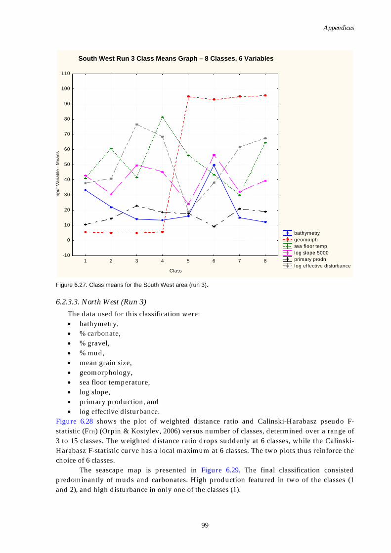
Appendices
99
South West (ED) 6 vars; Class; LS MeansWilks lambda=.00097, F(42, 1358E3)=1096E2, p=0.0000
bathymetry geomorph sea floor temp log slope 5000 primary prodn log effective disturbance
1 2 3 4 5 6 7 8
Class
-10
0
10
20
30
40
50
60
70
80
90
100
110
Figure 6.27. Class means for the South West area (run 3).
6.2.3.3. North West (Run 3) The data used for this classification were: • bathymetry, • % carbonate, • % gravel, • % mud, • mean grain size, • geomorphology, • sea floor temperature, • log slope, • primary production, and • log effective disturbance.
Figure 6.28 shows the plot of weighted distance ratio and Calinski-Harabasz pseudo F-statistic (FCH) (Orpin & Kostylev, 2006) versus number of classes, determined over a range of 3 to 15 classes. The weighted distance ratio drops suddenly at 6 classes, while the Calinski-Harabasz F-statistic curve has a local maximum at 6 classes. The two plots thus reinforce the choice of 6 classes.
The seascape map is presented in Figure 6.29. The final classification consisted predominantly of muds and carbonates. High production featured in two of the classes (1 and 2), and high disturbance in only one of the classes (1).
Inpu
t Var
iabl
e - M
eans
South West Run 3 Class Means Graph – 8 Classes, 6 Variables
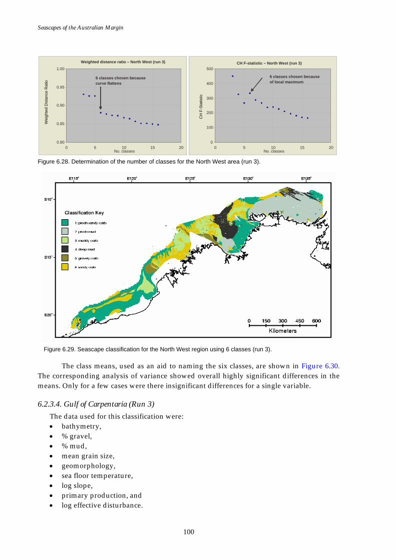
Seascapes of the Australian Margin
100
Figure 6.28. Determination of the number of classes for the North West area (run 3).
Figure 6.29. Seascape classification for the North West region using 6 classes (run 3).
The class means, used as an aid to naming the six classes, are shown in Figure 6.30. The corresponding analysis of variance showed overall highly significant differences in the means. Only for a few cases were there insignificant differences for a single variable.
6.2.3.4. Gulf of Carpentaria (Run 3) The data used for this classification were: • bathymetry, • % gravel, • % mud, • mean grain size, • geomorphology, • sea floor temperature, • log slope, • primary production, and • log effective disturbance.
Weighted distance ratio – North West (run 3)
0.80
0.85
0.90
0.95
1.00
0 5 10 15 20No. classes
6 classes chosen because curve flattens
Wei
ghte
d D
ista
nce
Rat
io
CH F-statistic – North West (run 3)
0
100
200
300
400
500
0 5 10 15 20No. classes
6 classes chosen because of local maximum
CH
F-S
tatis
tic
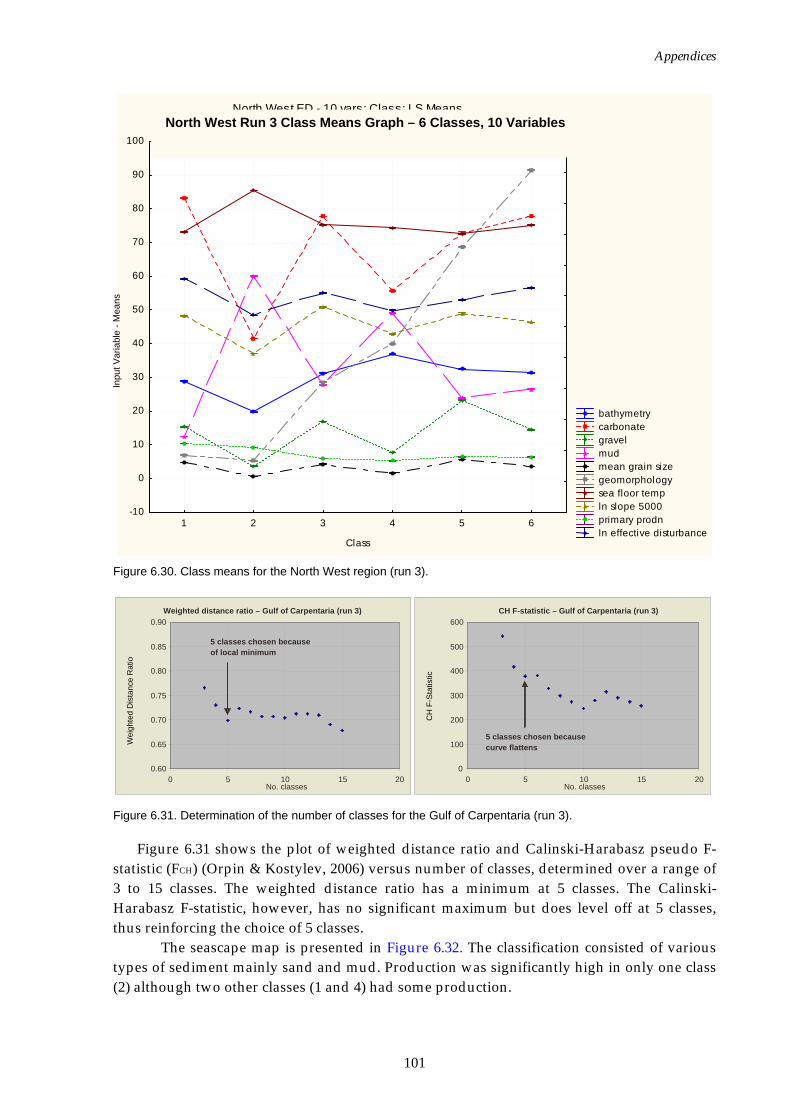
Appendices
101
North West ED - 10 vars; Class; LS MeansWilks lambda=.02837, F(50, 2216E3)=52477., p=0.0000
bathymetry carbonate gravel mud mean grain size geomorphology sea floor temp ln slope 5000 primary prodn ln effective disturbance
1 2 3 4 5 6
Class
-10
0
10
20
30
40
50
60
70
80
90
100
Figure 6.30. Class means for the North West region (run 3).
Figure 6.31. Determination of the number of classes for the Gulf of Carpentaria (run 3).
Figure 6.31 shows the plot of weighted distance ratio and Calinski-Harabasz pseudo F-statistic (FCH) (Orpin & Kostylev, 2006) versus number of classes, determined over a range of 3 to 15 classes. The weighted distance ratio has a minimum at 5 classes. The Calinski-Harabasz F-statistic, however, has no significant maximum but does level off at 5 classes, thus reinforcing the choice of 5 classes.
The seascape map is presented in Figure 6.32. The classification consisted of various types of sediment mainly sand and mud. Production was significantly high in only one class (2) although two other classes (1 and 4) had some production.
Weighted distance ratio – Gulf of Carpentaria (run 3)
0.60 0.65
0.70 0.75
0.80 0.85
0.90
0 5 10 15 20No. classes
5 classes chosen because of local minimum
Wei
ghte
d D
ista
nce
Rat
io
CH F-statistic – Gulf of Carpentaria (run 3)
0
100
200
300
400
500
600
0 5 10 15 20No. classes
5 classes chosen because curve flattens
CH
F-S
tatis
tic
Inpu
t Var
iabl
e - M
eans
North West Run 3 Class Means Graph – 6 Classes, 10 Variables
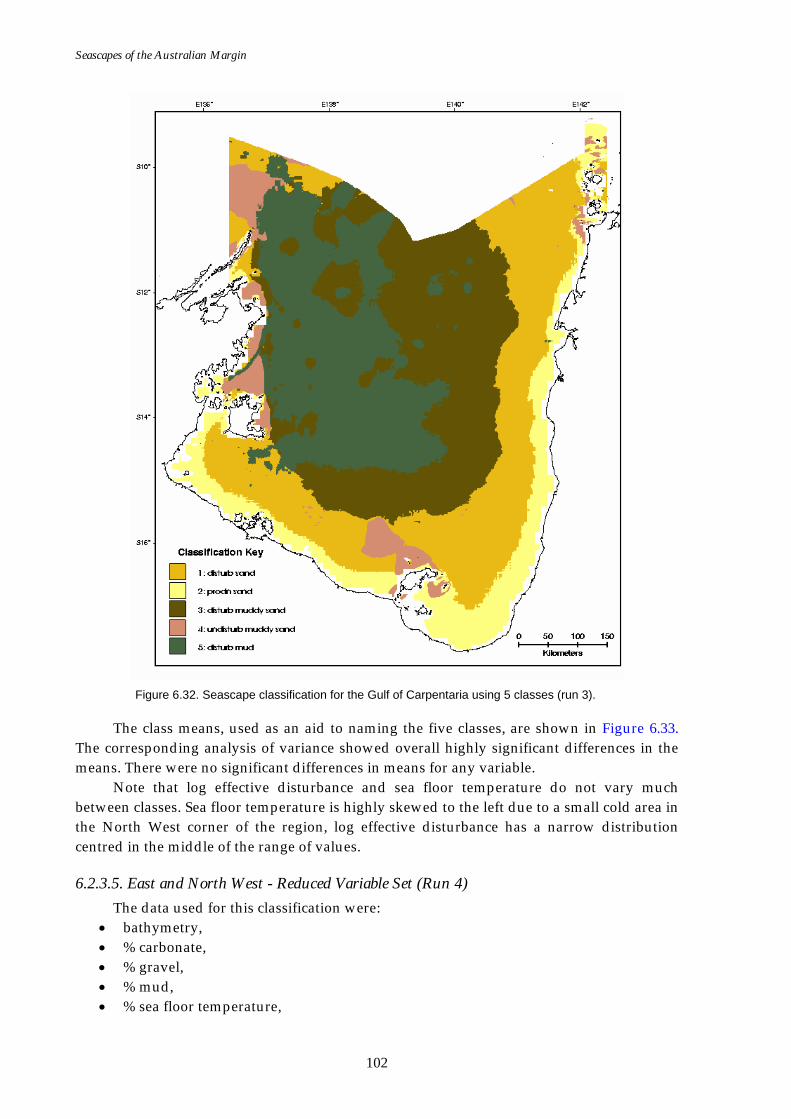
Seascapes of the Australian Margin
102
Figure 6.32. Seascape classification for the Gulf of Carpentaria using 5 classes (run 3).
The class means, used as an aid to naming the five classes, are shown in Figure 6.33. The corresponding analysis of variance showed overall highly significant differences in the means. There were no significant differences in means for any variable.
Note that log effective disturbance and sea floor temperature do not vary much between classes. Sea floor temperature is highly skewed to the left due to a small cold area in the North West corner of the region, log effective disturbance has a narrow distribution centred in the middle of the range of values.
6.2.3.5. East and North West - Reduced Variable Set (Run 4) The data used for this classification were:
• bathymetry, • % carbonate, • % gravel, • % mud, • % sea floor temperature,
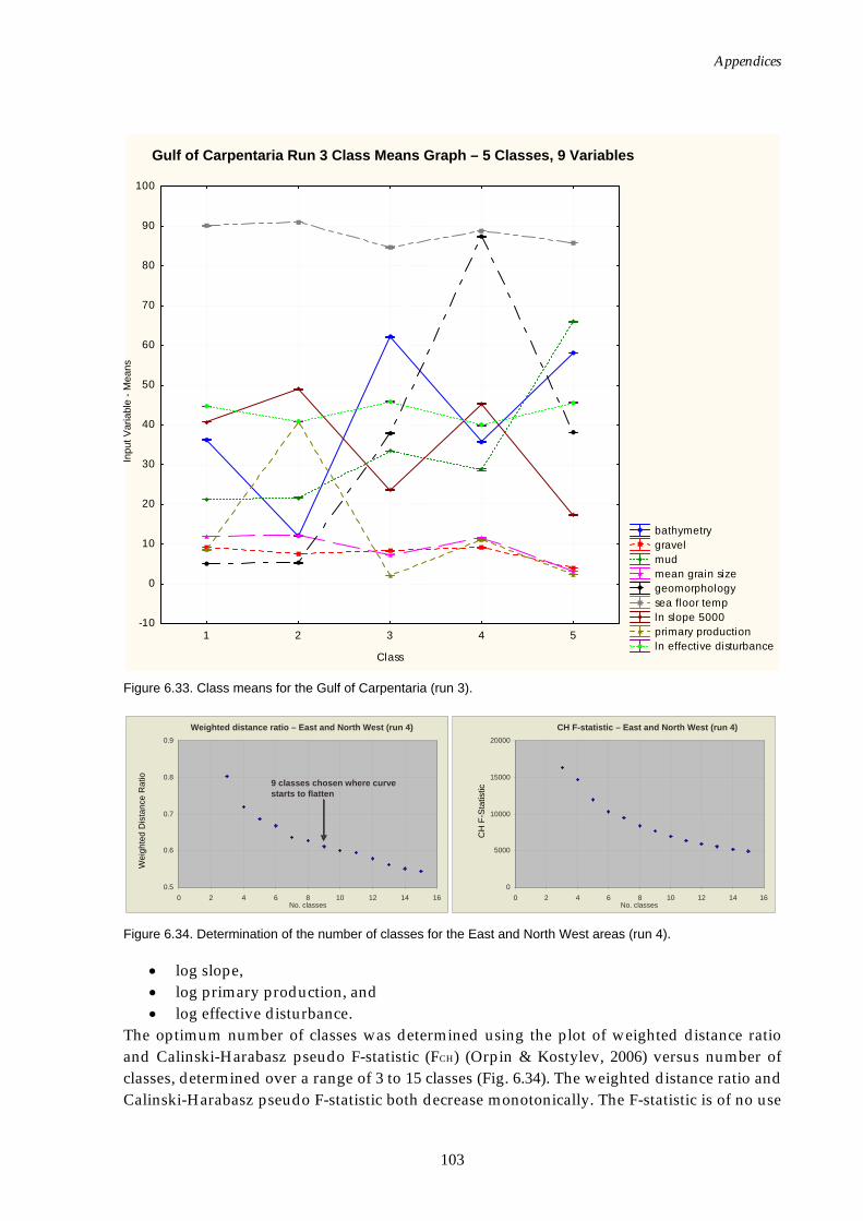
Appendices
103
Gulf of Carpentaria (ED) - 9 vars; Class; LS MeansWilks lambda=.00519, F(36, 1253E3)=1069E2, p=0.0000
bathymetry gravel mud mean grain size geomorphology sea floor temp ln slope 5000 primary production ln effective disturbance
1 2 3 4 5
Class
-10
0
10
20
30
40
50
60
70
80
90
100
Figure 6.33. Class means for the Gulf of Carpentaria (run 3).
Figure 6.34. Determination of the number of classes for the East and North West areas (run 4).
• log slope, • log primary production, and • log effective disturbance.
The optimum number of classes was determined using the plot of weighted distance ratio and Calinski-Harabasz pseudo F-statistic (FCH) (Orpin & Kostylev, 2006) versus number of classes, determined over a range of 3 to 15 classes (Fig. 6.34). The weighted distance ratio and Calinski-Harabasz pseudo F-statistic both decrease monotonically. The F-statistic is of no use
Weighted distance ratio – East and North West (run 4)
0.5
0.6
0.7
0.8
0.9
0 2 4 6 8 10 12 14 16No. classes
9 classes chosen where curve starts to flatten
Wei
ghte
d D
ista
nce
Rat
io
CH F-statistic – East and North West (run 4)
0
5000
10000
15000
20000
0 2 4 6 8 10 12 14 16No. classes
CH
F-S
tatis
tic
Inpu
t Var
iabl
e - M
eans
Gulf of Carpentaria Run 3 Class Means Graph – 5 Classes, 9 Variables
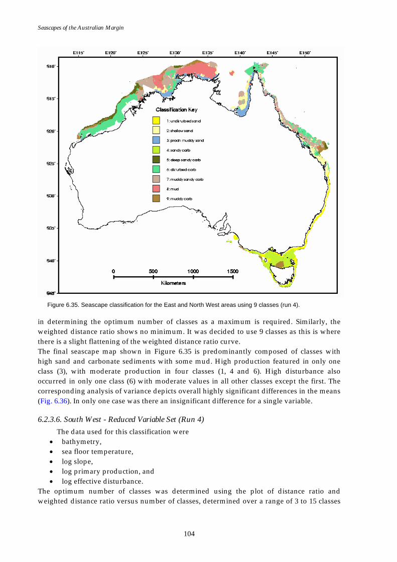
Seascapes of the Australian Margin
104
Figure 6.35. Seascape classification for the East and North West areas using 9 classes (run 4).
in determining the optimum number of classes as a maximum is required. Similarly, the weighted distance ratio shows no minimum. It was decided to use 9 classes as this is where there is a slight flattening of the weighted distance ratio curve. The final seascape map shown in Figure 6.35 is predominantly composed of classes with high sand and carbonate sediments with some mud. High production featured in only one class (3), with moderate production in four classes (1, 4 and 6). High disturbance also occurred in only one class (6) with moderate values in all other classes except the first. The corresponding analysis of variance depicts overall highly significant differences in the means (Fig. 6.36). In only one case was there an insignificant difference for a single variable.
6.2.3.6. South West - Reduced Variable Set (Run 4) The data used for this classification were
• bathymetry, • sea floor temperature, • log slope, • log primary production, and • log effective disturbance.
The optimum number of classes was determined using the plot of distance ratio and weighted distance ratio versus number of classes, determined over a range of 3 to 15 classes
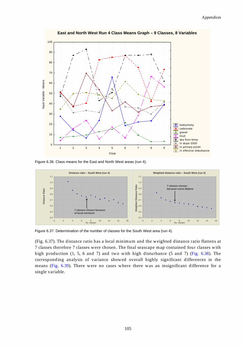
Appendices
105
East & NorthWest ED; Class; LS MeansWilks lambda=.00218, F(64, 5672E3)=1678E2, p=0.0000
bathymetry carbonate gravel mud sea floor temp ln slope 5000 ln primary prodn ln effective disturbance
1 2 3 4 5 6 7 8 9
Class
0
10
20
30
40
50
60
70
80
90
100
Figure 6.36. Class means for the East and North West areas (run 4).
Figure 6.37. Determination of the number of classes for the South West area (run 4).
(Fig. 6.37). The distance ratio has a local minimum and the weighted distance ratio flattens at 7 classes therefore 7 classes were chosen. The final seascape map contained four classes with high production (1, 5, 6 and 7) and two with high disturbance (5 and 7) (Fig. 6.38). The corresponding analysis of variance showed overall highly significant differences in the means (Fig. 6.39). There were no cases where there was an insignificant difference for a single variable.
Distance ratio – South West (run 4)
0.4 0.5 0.6 0.7 0.8 0.9 1.0 1.1
0 2 4 6 8 10 12 14 16No. classes
7 classes chosen because of local minimum
Dis
tanc
e R
atio
Weighted distance ratio – South West (run 4)
0.4
0.5
0.6
0.7
0.8
0.9
1.0
1.1
0 2 4 6 8 10 12 14 16No. classes
7 classes chosen because curve flattens
Wei
ghte
d D
ista
nce
Rat
io
Inpu
t Var
iabl
e - M
eans
East and North West Run 4 Class Means Graph – 9 Classes, 8 Variables
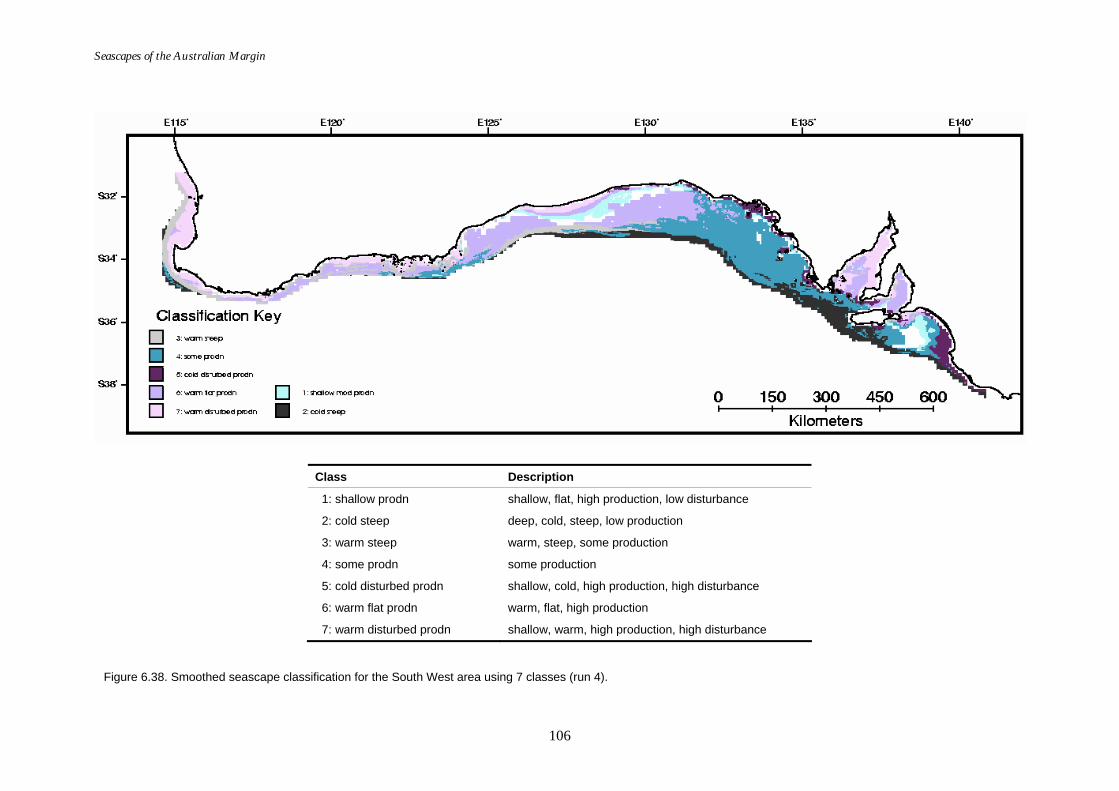
Seascapes of the Australian Margin
106
Class Description
1: shallow prodn shallow, flat, high production, low disturbance
2: cold steep deep, cold, steep, low production
3: warm steep warm, steep, some production
4: some prodn some production
5: cold disturbed prodn shallow, cold, high production, high disturbance
6: warm flat prodn warm, flat, high production
7: warm disturbed prodn shallow, warm, high production, high disturbance
Figure 6.38. Smoothed seascape classification for the South West area using 7 classes (run 4).
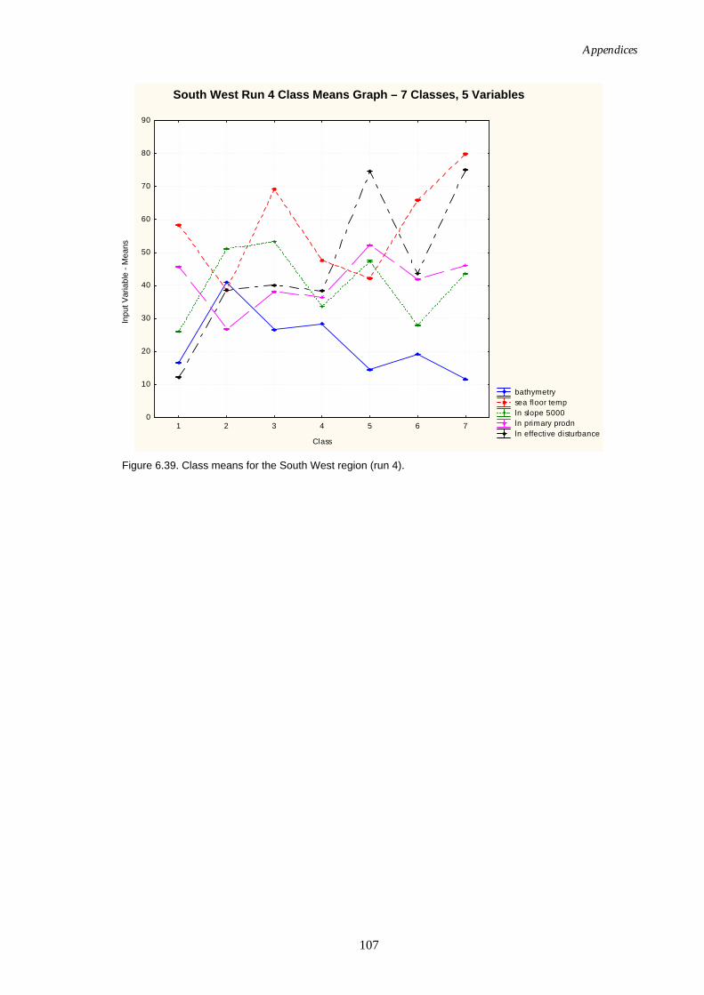
Appendices
107
SouthWest (ED2); Class; LS MeansWilks lambda=.01959, F(30, 1167E3)=65070., p=0.0000
bathymetry sea floor temp ln slope 5000 ln primary prodn ln effective disturbance
1 2 3 4 5 6 7
Class
0
10
20
30
40
50
60
70
80
90
Figure 6.39. Class means for the South West region (run 4).
Inpu
t Var
iabl
e - M
eans
South West Run 4 Class Means Graph – 7 Classes, 5 Variables
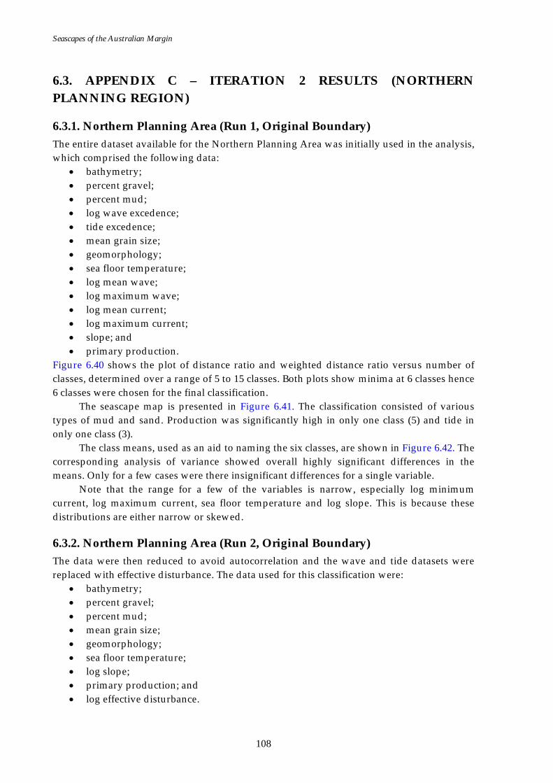
Seascapes of the Australian Margin
108
6.3. APPENDIX C – ITERATION 2 RESULTS (NORTHERN PLANNING REGION)
6.3.1. Northern Planning Area (Run 1, Original Boundary) The entire dataset available for the Northern Planning Area was initially used in the analysis, which comprised the following data:
• bathymetry; • percent gravel; • percent mud; • log wave excedence; • tide excedence; • mean grain size; • geomorphology; • sea floor temperature; • log mean wave; • log maximum wave; • log mean current; • log maximum current; • slope; and • primary production.
Figure 6.40 shows the plot of distance ratio and weighted distance ratio versus number of classes, determined over a range of 5 to 15 classes. Both plots show minima at 6 classes hence 6 classes were chosen for the final classification.
The seascape map is presented in Figure 6.41. The classification consisted of various types of mud and sand. Production was significantly high in only one class (5) and tide in only one class (3).
The class means, used as an aid to naming the six classes, are shown in Figure 6.42. The corresponding analysis of variance showed overall highly significant differences in the means. Only for a few cases were there insignificant differences for a single variable.
Note that the range for a few of the variables is narrow, especially log minimum current, log maximum current, sea floor temperature and log slope. This is because these distributions are either narrow or skewed.
6.3.2. Northern Planning Area (Run 2, Original Boundary) The data were then reduced to avoid autocorrelation and the wave and tide datasets were replaced with effective disturbance. The data used for this classification were:
• bathymetry; • percent gravel; • percent mud; • mean grain size; • geomorphology; • sea floor temperature; • log slope; • primary production; and • log effective disturbance.
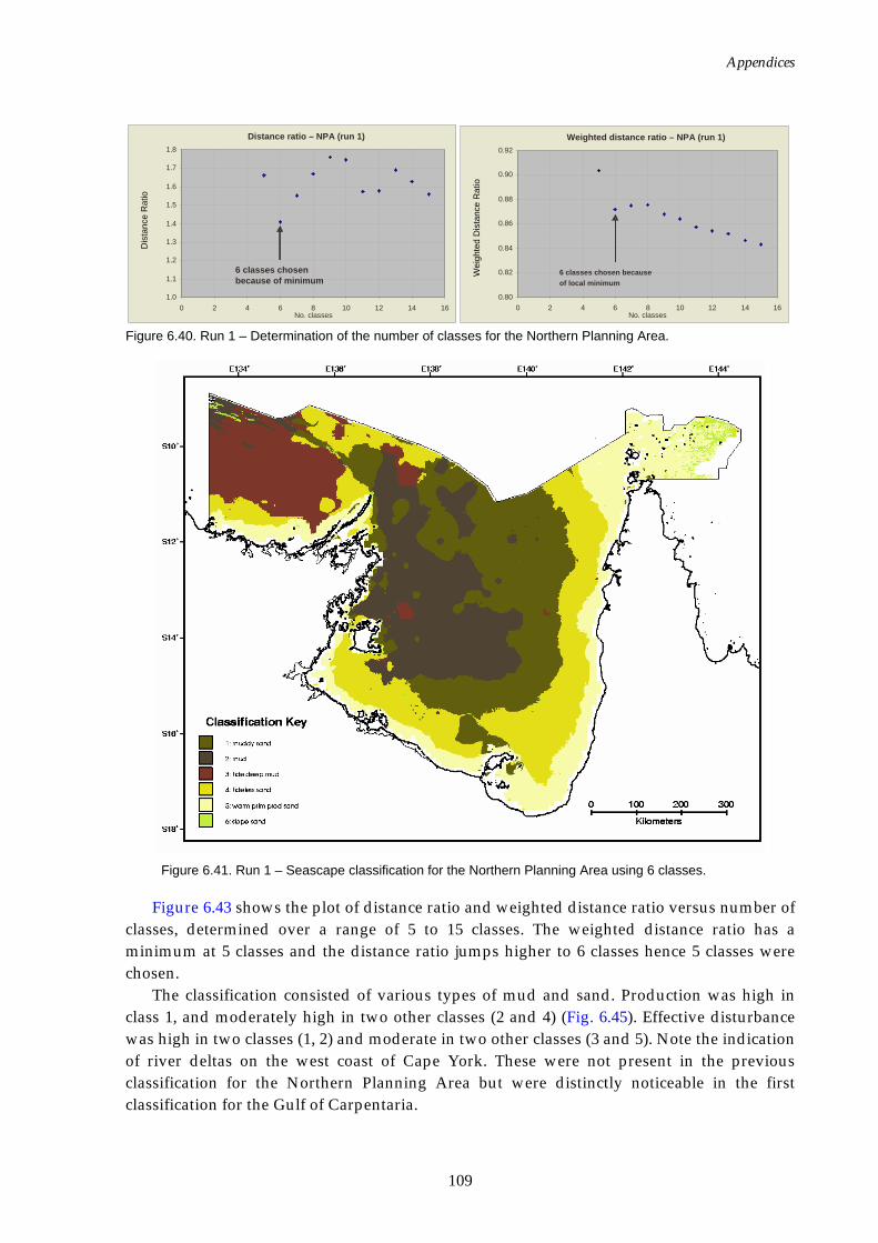
Appendices
109
Figure 6.40. Run 1 – Determination of the number of classes for the Northern Planning Area.
Figure 6.41. Run 1 – Seascape classification for the Northern Planning Area using 6 classes.
Figure 6.43 shows the plot of distance ratio and weighted distance ratio versus number of classes, determined over a range of 5 to 15 classes. The weighted distance ratio has a minimum at 5 classes and the distance ratio jumps higher to 6 classes hence 5 classes were chosen.
The classification consisted of various types of mud and sand. Production was high in class 1, and moderately high in two other classes (2 and 4) (Fig. 6.45). Effective disturbance was high in two classes (1, 2) and moderate in two other classes (3 and 5). Note the indication of river deltas on the west coast of Cape York. These were not present in the previous classification for the Northern Planning Area but were distinctly noticeable in the first classification for the Gulf of Carpentaria.
Distance ratio – NPA (run 1)
1.0 1.1 1.2 1.3 1.4 1.5 1.6 1.7 1.8
0 2 4 6 8 10 12 14 16No. classes
6 classes chosen because of minimum
Dis
tanc
e R
atio
Weighted distance ratio – NPA (run 1)
0.80
0.82
0.84
0.86
0.88
0.90
0.92
0 2 4 6 8 10 12 14 16No. classes
6 classes chosen because of local minimum
Wei
ghte
d D
ista
nce
Rat
io
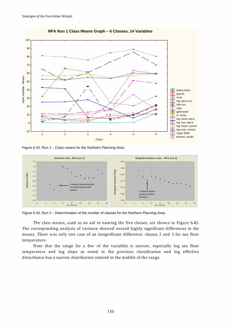
Seascapes of the Australian Margin
110
Northern planning area - 14 v ariables - 6 classes
Wilks lambda=.00421, F(70, 2032E3)=62554., p=0.0000
bathy metry grav el mud log wav e exc tide exc mgs geomorph sf temp log mean wav e log max wav e log mean current log max current slope 5000 primary prodn
1 2 3 4 5 6
Class
-10
0
10
20
30
40
50
60
70
80
90
100
Figure 6.42. Run 1 – Class means for the Northern Planning Area.
Figure 6.43. Run 2 – Determination of the number of classes for the Northern Planning Area.
The class means, used as an aid to naming the five classes, are shown in Figure 6.45. The corresponding analysis of variance showed overall highly significant differences in the means. There was only one case of an insignificant difference: classes 2 and 3 for sea floor temperature.
Note that the range for a few of the variables is narrow, especially log sea floor temperature and log slope as noted in the previous classification and log effective disturbance has a narrow distribution centred in the middle of the range.
Distance ratio - NPA (run 2)
0.5 0.6 0.7 0.8 0.9 1.0 1.1 1.2 1.3
0 2 4 6 8 10 12 14 16No. classes
5 classes chosen because of sudden jump up at 6 classes D
ista
nce
Rat
io
Weighted distance ratio – NPA (run 2)
0.60
0.65
0.70
0.75
0.80
0.85
0.90
0 2 4 6 8 10 12 14 16No. classes
5 classes chosen because of local minimum
Wei
ghte
d D
ista
nce
Rat
io
Inpu
t Var
iabl
e - M
eans
NPA Run 1 Class Means Graph – 6 Classes, 14 Variables
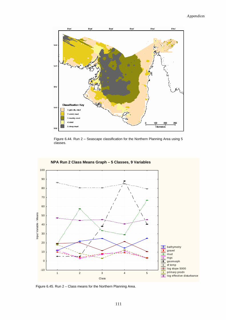
Appendices
111
Figure 6.44. Run 2 – Seascape classification for the Northern Planning Area using 5 classes.
Northern Planning Area (9 vars with effective disturbance and log slope) Class; LS MeansWilks lambda=.00933, F(36, 1602E3)=1104E2, p=0.0000
bathymetry gravel mud mgs geomorph sf temp log slope 5000 primary prodn log effective disturbance
1 2 3 4 5
Class
-10
0
10
20
30
40
50
60
70
80
90
100
Figure 6.45. Run 2 – Class means for the Northern Planning Area.
Inpu
t Var
iabl
e - M
eans
NPA Run 2 Class Means Graph – 5 Classes, 9 Variables
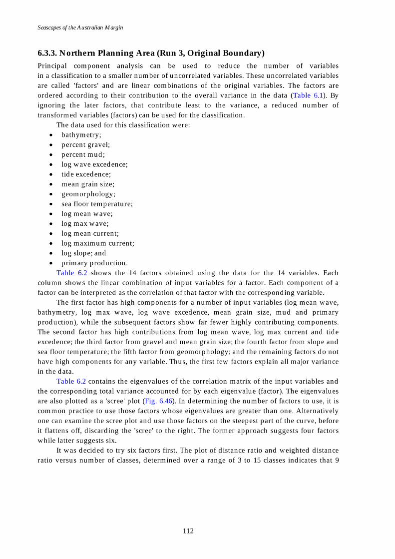
Seascapes of the Australian Margin
112
6.3.3. Northern Planning Area (Run 3, Original Boundary) Principal component analysis can be used to reduce the number of variables in a classification to a smaller number of uncorrelated variables. These uncorrelated variables are called 'factors' and are linear combinations of the original variables. The factors are ordered according to their contribution to the overall variance in the data (Table 6.1). By ignoring the later factors, that contribute least to the variance, a reduced number of transformed variables (factors) can be used for the classification.
The data used for this classification were: • bathymetry; • percent gravel; • percent mud; • log wave excedence; • tide excedence; • mean grain size; • geomorphology; • sea floor temperature; • log mean wave; • log max wave; • log mean current; • log maximum current; • log slope; and • primary production.
Table 6.2 shows the 14 factors obtained using the data for the 14 variables. Each column shows the linear combination of input variables for a factor. Each component of a factor can be interpreted as the correlation of that factor with the corresponding variable.
The first factor has high components for a number of input variables (log mean wave, bathymetry, log max wave, log wave excedence, mean grain size, mud and primary production), while the subsequent factors show far fewer highly contributing components. The second factor has high contributions from log mean wave, log max current and tide excedence; the third factor from gravel and mean grain size; the fourth factor from slope and sea floor temperature; the fifth factor from geomorphology; and the remaining factors do not have high components for any variable. Thus, the first few factors explain all major variance in the data.
Table 6.2 contains the eigenvalues of the correlation matrix of the input variables and the corresponding total variance accounted for by each eigenvalue (factor). The eigenvalues are also plotted as a 'scree' plot (Fig. 6.46). In determining the number of factors to use, it is common practice to use those factors whose eigenvalues are greater than one. Alternatively one can examine the scree plot and use those factors on the steepest part of the curve, before it flattens off, discarding the 'scree' to the right. The former approach suggests four factors while latter suggests six.
It was decided to try six factors first. The plot of distance ratio and weighted distance ratio versus number of classes, determined over a range of 3 to 15 classes indicates that 9
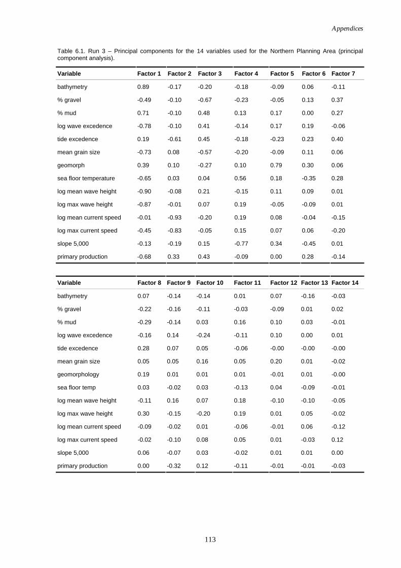
Appendices
113
Table 6.1. Run 3 – Principal components for the 14 variables used for the Northern Planning Area (principal component analysis).
Variable Factor 1 Factor 2 Factor 3 Factor 4 Factor 5 Factor 6 Factor 7
bathymetry 0.89 -0.17 -0.20 -0.18 -0.09 0.06 -0.11
% gravel -0.49 -0.10 -0.67 -0.23 -0.05 0.13 0.37
% mud 0.71 -0.10 0.48 0.13 0.17 0.00 0.27
log wave excedence -0.78 -0.10 0.41 -0.14 0.17 0.19 -0.06
tide excedence 0.19 -0.61 0.45 -0.18 -0.23 0.23 0.40
mean grain size -0.73 0.08 -0.57 -0.20 -0.09 0.11 0.06
geomorph 0.39 0.10 -0.27 0.10 0.79 0.30 0.06
sea floor temperature -0.65 0.03 0.04 0.56 0.18 -0.35 0.28
log mean wave height -0.90 -0.08 0.21 -0.15 0.11 0.09 0.01
log max wave height -0.87 -0.01 0.07 0.19 -0.05 -0.09 0.01
log mean current speed -0.01 -0.93 -0.20 0.19 0.08 -0.04 -0.15
log max current speed -0.45 -0.83 -0.05 0.15 0.07 0.06 -0.20
slope 5,000 -0.13 -0.19 0.15 -0.77 0.34 -0.45 0.01
primary production -0.68 0.33 0.43 -0.09 0.00 0.28 -0.14
Variable Factor 8 Factor 9 Factor 10 Factor 11 Factor 12 Factor 13 Factor 14
bathymetry 0.07 -0.14 -0.14 0.01 0.07 -0.16 -0.03
% gravel -0.22 -0.16 -0.11 -0.03 -0.09 0.01 0.02
% mud -0.29 -0.14 0.03 0.16 0.10 0.03 -0.01
log wave excedence -0.16 0.14 -0.24 -0.11 0.10 0.00 0.01
tide excedence 0.28 0.07 0.05 -0.06 -0.00 -0.00 -0.00
mean grain size 0.05 0.05 0.16 0.05 0.20 0.01 -0.02
geomorphology 0.19 0.01 0.01 0.01 -0.01 0.01 -0.00
sea floor temp 0.03 -0.02 0.03 -0.13 0.04 -0.09 -0.01
log mean wave height -0.11 0.16 0.07 0.18 -0.10 -0.10 -0.05
log max wave height 0.30 -0.15 -0.20 0.19 0.01 0.05 -0.02
log mean current speed -0.09 -0.02 0.01 -0.06 -0.01 0.06 -0.12
log max current speed -0.02 -0.10 0.08 0.05 0.01 -0.03 0.12
slope 5,000 0.06 -0.07 0.03 -0.02 0.01 0.01 0.00
primary production 0.00 -0.32 0.12 -0.11 -0.01 -0.01 -0.03
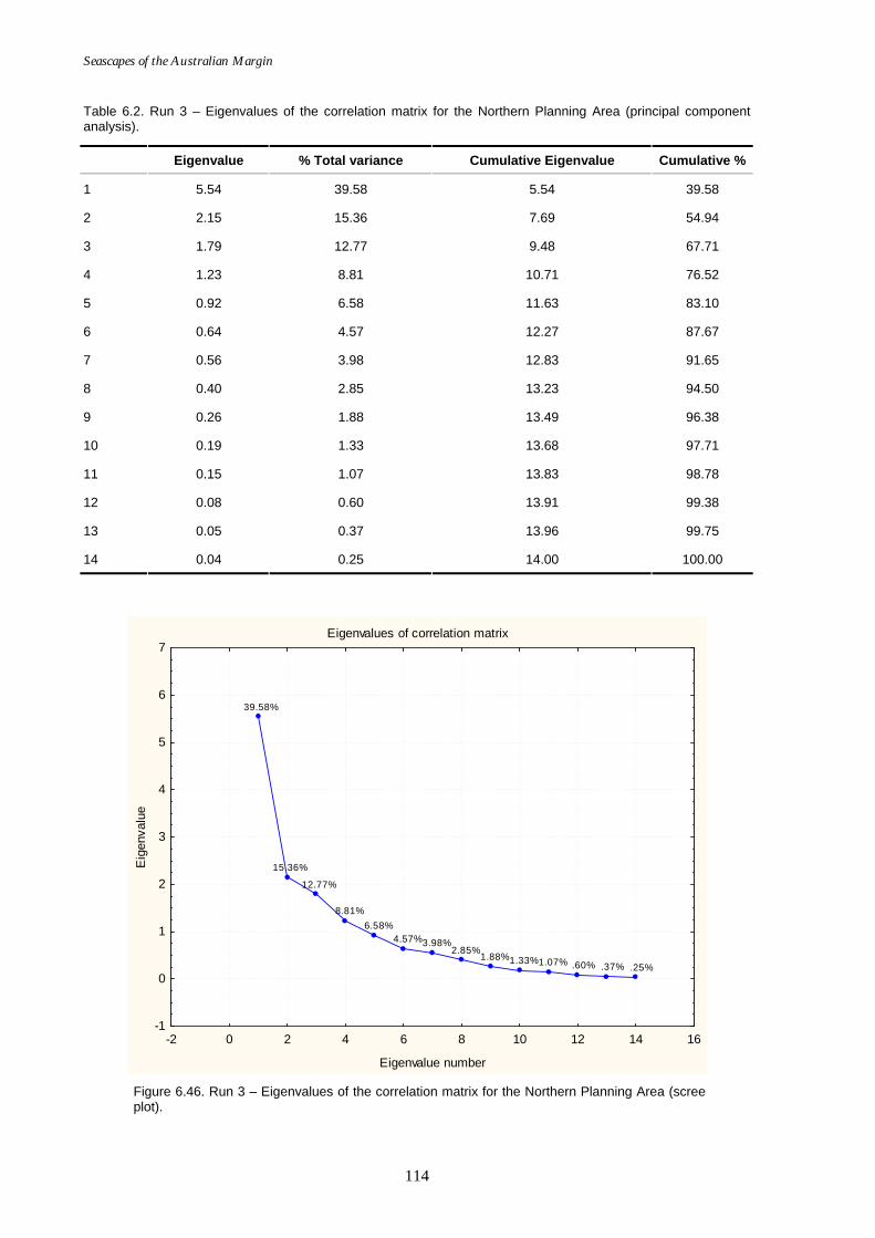
Seascapes of the Australian Margin
114
Table 6.2. Run 3 – Eigenvalues of the correlation matrix for the Northern Planning Area (principal component analysis).
Eigenvalue % Total variance Cumulative Eigenvalue Cumulative %
1 5.54 39.58 5.54 39.58
2 2.15 15.36 7.69 54.94
3 1.79 12.77 9.48 67.71
4 1.23 8.81 10.71 76.52
5 0.92 6.58 11.63 83.10
6 0.64 4.57 12.27 87.67
7 0.56 3.98 12.83 91.65
8 0.40 2.85 13.23 94.50
9 0.26 1.88 13.49 96.38
10 0.19 1.33 13.68 97.71
11 0.15 1.07 13.83 98.78
12 0.08 0.60 13.91 99.38
13 0.05 0.37 13.96 99.75
14 0.04 0.25 14.00 100.00
Eigenvalues of correlation matrix
39.58%
15.36%
12.77%
8.81% 6.58%
4.57% 3.98% 2.85%
1.88% 1.33% 1.07% .60% .37% .25%
-2 0 2 4 6 8 10 12 14 16
Eigenvalue number
-1
0
1
2
3
4
5
6
7
Eig
enva
lue
Figure 6.46. Run 3 – Eigenvalues of the correlation matrix for the Northern Planning Area (scree plot).
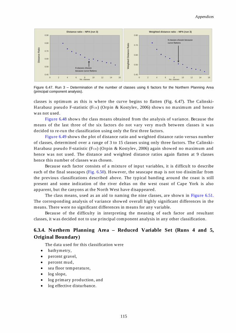
Appendices
115
Figure 6.47. Run 3 – Determination of the number of classes using 6 factors for the Northern Planning Area (principal component analysis).
classes is optimum as this is where the curve begins to flatten (Fig. 6.47). The Calinski-Harabasz pseudo F-statistic (FCH) (Orpin & Kostylev, 2006) shows no maximum and hence was not used.
Figure 6.48 shows the class means obtained from the analysis of variance. Because the means of the last three of the six factors do not vary very much between classes it was decided to re-run the classification using only the first three factors.
Figure 6.49 shows the plot of distance ratio and weighted distance ratio versus number of classes, determined over a range of 3 to 15 classes using only three factors. The Calinski-Harabasz pseudo F-statistic (FCH) (Orpin & Kostylev, 2006) again showed no maximum and hence was not used. The distance and weighted distance ratios again flatten at 9 classes hence this number of classes was chosen.
Because each factor consists of a mixture of input variables, it is difficult to describe each of the final seascapes (Fig. 6.50). However, the seascape map is not too dissimilar from the previous classifications described above. The typical banding around the coast is still present and some indication of the river deltas on the west coast of Cape York is also apparent, but the canyons at the North West have disappeared.
The class means, used as an aid to naming the nine classes, are shown in Figure 6.51. The corresponding analysis of variance showed overall highly significant differences in the means. There were no significant differences in means for any variable.
Because of the difficulty in interpreting the meaning of each factor and resultant classes, it was decided not to use principal component analysis in any other classification.
6.3.4. Northern Planning Area – Reduced Variable Set (Runs 4 and 5, Original Boundary)
The data used for this classification were • bathymetry, • percent gravel, • percent mud, • sea floor temperature, • log slope, • log primary production, and • log effective disturbance.
Distance ratio – NPA (run 3)
0.40
0.50
0.60
0.70
0.80
0.90
0 2 4 6 8 10 12 14 16No. classes
9 classes chosen because curve flattens
Dis
tanc
e R
atio
Weighted distance ratio – NPA (run 3)
0.40
0.50
0.60
0.70
0.80
0 2 4 6 8 10 12 14 16No. classes
9 classes chosen because curve flattens
Wei
ghte
d D
ista
nce
Rat
io
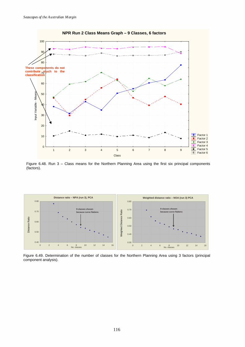
Seascapes of the Australian Margin
116
Figure 6.48. Run 3 – Class means for the Northern Planning Area using the first six principal components (factors).
Figure 6.49. Determination of the number of classes for the Northern Planning Area using 3 factors (principal component analysis).
Northern Planning Area - Principal Component Analysis Class; LS MeansWilks lambda=.00381, F(48, 2101E3)=92004., p=0.0000
Factor 1 Factor 2 Factor 3 Factor 4 Factor 5 Factor 6
1 2 3 4 5 6 7 8 9
Class
0
10
20
30
40
50
60
70
80
90
100
These components do not contribute much to the classification
Inpu
t Var
iabl
e - M
eans
NPR Run 2 Class Means Graph – 9 Classes, 6 factors
Distance ratio – NPA (run 3), PCA
0.40
0.50
0.60
0.70
0.80
0 2 4 6 8 10 12 14 16No. classes
9 classes chosen because curve flattens
Dis
tanc
e R
atio
Weighted distance ratio – NOA (run 3) PCA
0.30
0.40
0.50
0.60
0.70
0.80
0 2 4 6 8 10 12 14 16No. classes
9 classes chosen because curve flattens
Wei
ghte
d D
ista
nce
Rat
io
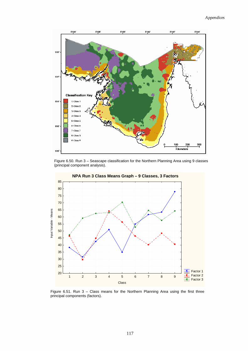
Appendices
117
Figure 6.50. Run 3 – Seascape classification for the Northern Planning Area using 9 classes (principal component analysis).
Northern Planning Area - 3 Factors; LS Means
Factor 1 Factor 2 Factor 3
1 2 3 4 5 6 7 8 9
Class
20
25
30
35
40
45
50
55
60
65
70
75
80
85
Figure 6.51. Run 3 – Class means for the Northern Planning Area using the first three principal components (factors).
Inpu
t Var
iabl
e - M
eans
NPA Run 3 Class Means Graph – 9 Classes, 3 Factors
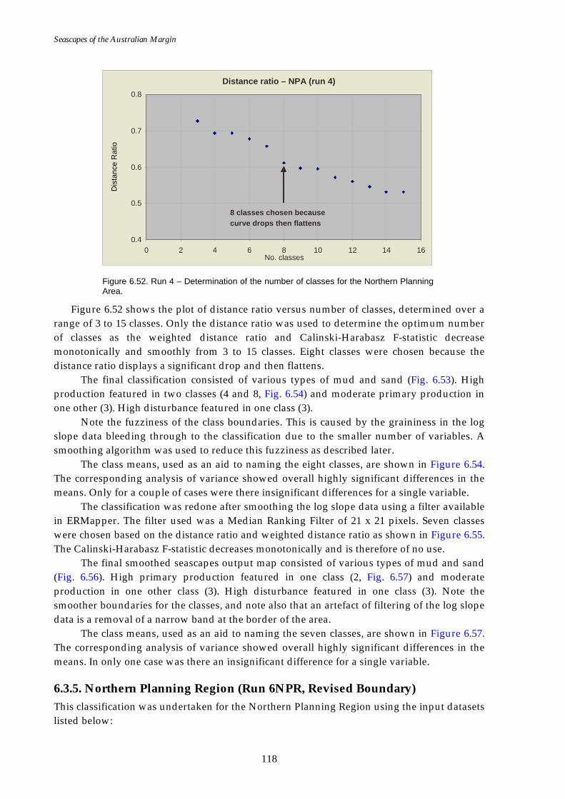
Seascapes of the Australian Margin
118
Figure 6.52. Run 4 – Determination of the number of classes for the Northern Planning Area.
Figure 6.52 shows the plot of distance ratio versus number of classes, determined over a range of 3 to 15 classes. Only the distance ratio was used to determine the optimum number of classes as the weighted distance ratio and Calinski-Harabasz F-statistic decrease monotonically and smoothly from 3 to 15 classes. Eight classes were chosen because the distance ratio displays a significant drop and then flattens.
The final classification consisted of various types of mud and sand (Fig. 6.53). High production featured in two classes (4 and 8, Fig. 6.54) and moderate primary production in one other (3). High disturbance featured in one class (3).
Note the fuzziness of the class boundaries. This is caused by the graininess in the log slope data bleeding through to the classification due to the smaller number of variables. A smoothing algorithm was used to reduce this fuzziness as described later.
The class means, used as an aid to naming the eight classes, are shown in Figure 6.54. The corresponding analysis of variance showed overall highly significant differences in the means. Only for a couple of cases were there insignificant differences for a single variable.
The classification was redone after smoothing the log slope data using a filter available in ERMapper. The filter used was a Median Ranking Filter of 21 x 21 pixels. Seven classes were chosen based on the distance ratio and weighted distance ratio as shown in Figure 6.55. The Calinski-Harabasz F-statistic decreases monotonically and is therefore of no use.
The final smoothed seascapes output map consisted of various types of mud and sand (Fig. 6.56). High primary production featured in one class (2, Fig. 6.57) and moderate production in one other class (3). High disturbance featured in one class (3). Note the smoother boundaries for the classes, and note also that an artefact of filtering of the log slope data is a removal of a narrow band at the border of the area.
The class means, used as an aid to naming the seven classes, are shown in Figure 6.57. The corresponding analysis of variance showed overall highly significant differences in the means. In only one case was there an insignificant difference for a single variable.
6.3.5. Northern Planning Region (Run 6NPR, Revised Boundary) This classification was undertaken for the Northern Planning Region using the input datasets listed below:
Distance ratio – NPA (run 4)
0.4
0.5
0.6
0.7
0.8
0 2 4 6 8 10 12 14 16 No. classes
8 classes chosen because curve drops then flattens
Dis
tanc
e R
atio
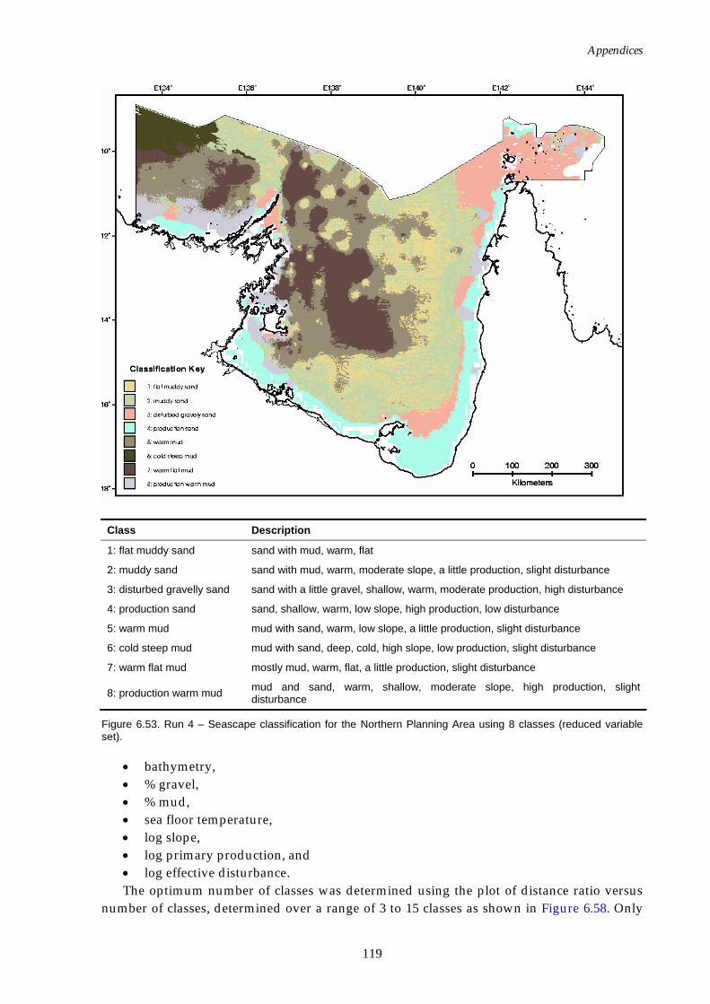
Appendices
119
Class Description
1: flat muddy sand sand with mud, warm, flat
2: muddy sand sand with mud, warm, moderate slope, a little production, slight disturbance
3: disturbed gravelly sand sand with a little gravel, shallow, warm, moderate production, high disturbance
4: production sand sand, shallow, warm, low slope, high production, low disturbance
5: warm mud mud with sand, warm, low slope, a little production, slight disturbance
6: cold steep mud mud with sand, deep, cold, high slope, low production, slight disturbance
7: warm flat mud mostly mud, warm, flat, a little production, slight disturbance
8: production warm mud mud and sand, warm, shallow, moderate slope, high production, slight disturbance
Figure 6.53. Run 4 – Seascape classification for the Northern Planning Area using 8 classes (reduced variable set).
• bathymetry, • % gravel, • % mud, • sea floor temperature, • log slope, • log primary production, and • log effective disturbance. The optimum number of classes was determined using the plot of distance ratio versus
number of classes, determined over a range of 3 to 15 classes as shown in Figure 6.58. Only
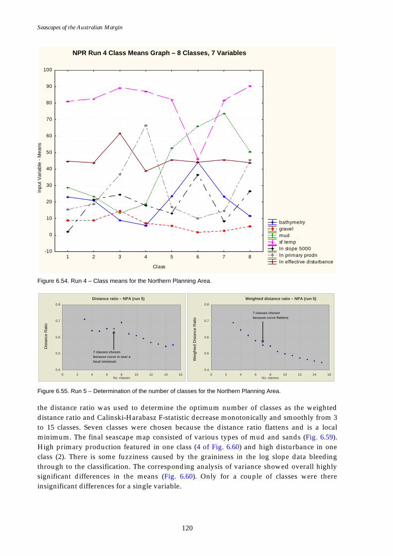
Seascapes of the Australian Margin
120
Northern Planning Area (ED2); Class; LS MeansWilks lambda=.00607, F(49, 2164E3)=76518., p=0.0000
bathymetry gravel mud sf temp ln slope 5000 ln primary prodn ln effective disturbance
1 2 3 4 5 6 7 8
Class
-10
0
10
20
30
40
50
60
70
80
90
100
Figure 6.54. Run 4 – Class means for the Northern Planning Area.
Figure 6.55. Run 5 – Determination of the number of classes for the Northern Planning Area.
the distance ratio was used to determine the optimum number of classes as the weighted distance ratio and Calinski-Harabasz F-statistic decrease monotonically and smoothly from 3 to 15 classes. Seven classes were chosen because the distance ratio flattens and is a local minimum. The final seascape map consisted of various types of mud and sands (Fig. 6.59). High primary production featured in one class (4 of Fig. 6.60) and high disturbance in one class (2). There is some fuzziness caused by the graininess in the log slope data bleeding through to the classification. The corresponding analysis of variance showed overall highly significant differences in the means (Fig. 6.60). Only for a couple of classes were there insignificant differences for a single variable.
Distance ratio – NPA (run 5)
0.4
0.5
0.6
0.7
0.8
0 2 4 6 8 10 12 14 16No. classes
7 classes chosen because curve is near a local minimum
Dis
tanc
e R
atio
Weighted distance ratio – NPA (run 5)
0.4
0.5
0.6
0.7
0.8
0 2 4 6 8 10 12 14 16No. classes
7 classes chosen because curve flattens
Wei
ghte
d D
ista
nce
Rat
io
Inpu
t Var
iabl
e - M
eans
NPR Run 4 Class Means Graph – 8 Classes, 7 Variables

Appendices
121
Class Description
1: sand sand, warm, a little production, slight disturbance
2: production sand sand, shallow, warm, high production, low disturbance
3: disturbed gravelly sand sand with a little gravel, shallow, warm, steep, moderate production, high disturbance
4: muddy sand sand with mud, warm, flat, low production
5: warm flat mud mostly mud, warm, flat, a little production, slight disturbance
6: cold steep mud mud with sand, deep, cold, high slope, low production, slight disturbance
7: warm mud mud with sand, warm, some production, slight disturbance
Figure 6.56. Run 5 – Smoothed seascape classification for the Northern Planning Area using 7 classes.
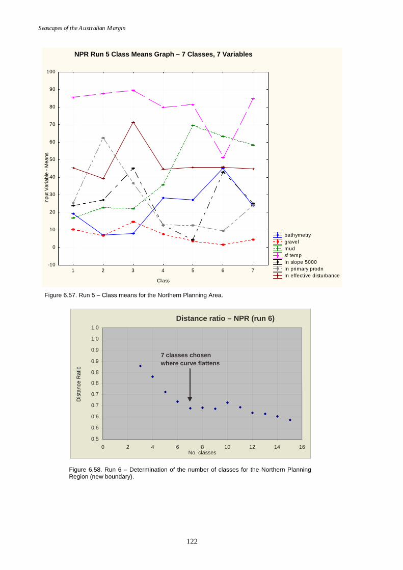
Seascapes of the Australian Margin
122
Northern Planning Area (ED2) filtered; Class; LS MeansWilks lambda=.00470, F(42, 1887E3)=95994., p=0.0000
bathymetry gravel mud sf temp ln slope 5000 ln primary prodn ln effective disturbance
1 2 3 4 5 6 7
Class
-10
0
10
20
30
40
50
60
70
80
90
100
Figure 6.57. Run 5 – Class means for the Northern Planning Area.
Figure 6.58. Run 6 – Determination of the number of classes for the Northern Planning Region (new boundary).
Distance ratio – NPR (run 6)
0.5 0.6 0.6 0.7 0.7 0.8 0.8 0.9 0.9 1.0 1.0
0 2 4 6 8 10 12 14 16 No. classes
7 classes chosen where curve flattens
Dis
tanc
e R
atio
Inpu
t Var
iabl
e - M
eans
NPR Run 5 Class Means Graph – 7 Classes, 7 Variables
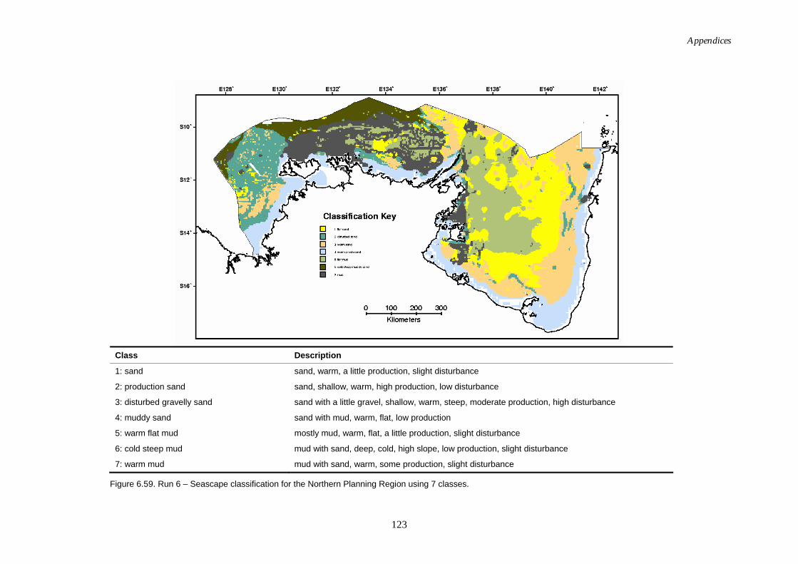
Appendices
123
Class Description
1: sand sand, warm, a little production, slight disturbance
2: production sand sand, shallow, warm, high production, low disturbance
3: disturbed gravelly sand sand with a little gravel, shallow, warm, steep, moderate production, high disturbance
4: muddy sand sand with mud, warm, flat, low production
5: warm flat mud mostly mud, warm, flat, a little production, slight disturbance
6: cold steep mud mud with sand, deep, cold, high slope, low production, slight disturbance
7: warm mud mud with sand, warm, some production, slight disturbance
Figure 6.59. Run 6 – Seascape classification for the Northern Planning Region using 7 classes.
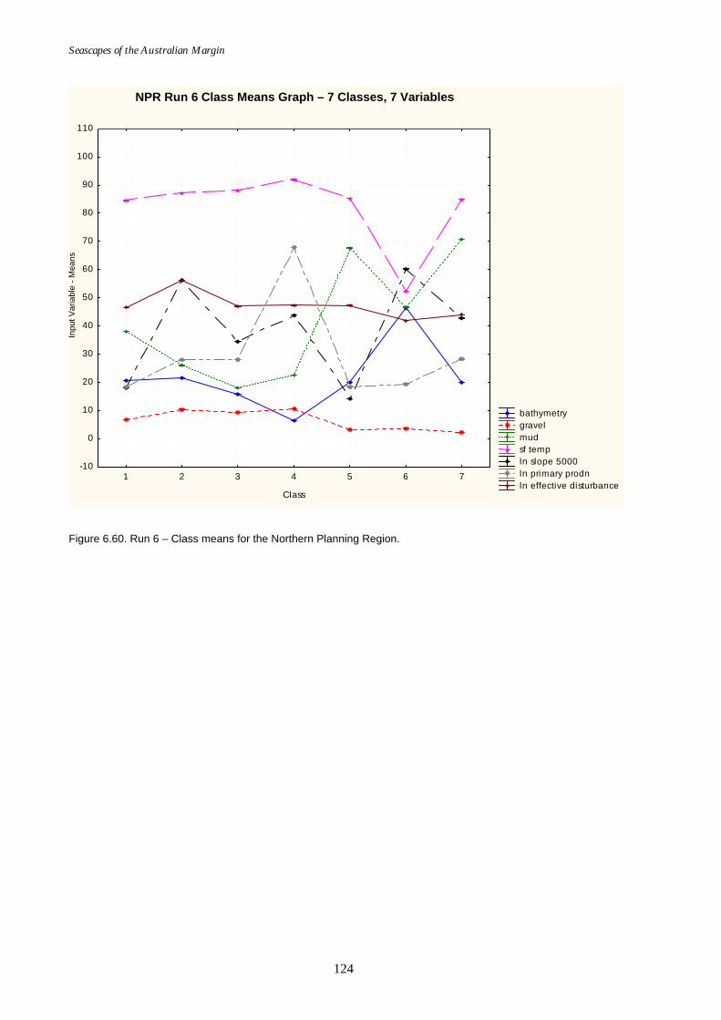
Seascapes of the Australian Margin
124
New Northern Planning Area (ED2);Class; LS MeansWilks lambda=.00883, F(42, 2543E3)=1054E2, p=0.0000
bathymetry gravel mud sf temp ln slope 5000 ln primary prodn ln effective disturbance
1 2 3 4 5 6 7
Class
-10
0
10
20
30
40
50
60
70
80
90
100
110
Figure 6.60. Run 6 – Class means for the Northern Planning Region.
Inpu
t Var
iabl
e - M
eans
NPR Run 6 Class Means Graph – 7 Classes, 7 Variables
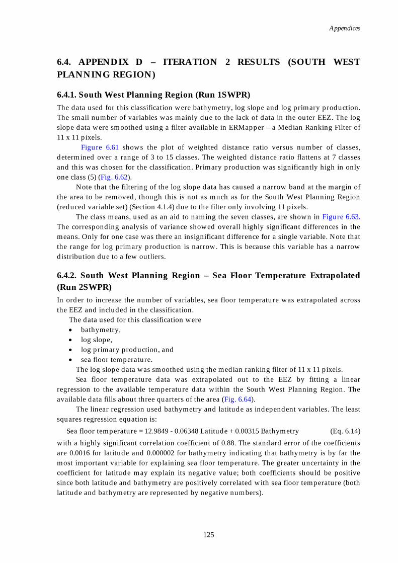
Appendices
125
6.4. APPENDIX D – ITERATION 2 RESULTS (SOUTH WEST PLANNING REGION)
6.4.1. South West Planning Region (Run 1SWPR) The data used for this classification were bathymetry, log slope and log primary production. The small number of variables was mainly due to the lack of data in the outer EEZ. The log slope data were smoothed using a filter available in ERMapper – a Median Ranking Filter of 11 x 11 pixels.
Figure 6.61 shows the plot of weighted distance ratio versus number of classes, determined over a range of 3 to 15 classes. The weighted distance ratio flattens at 7 classes and this was chosen for the classification. Primary production was significantly high in only one class (5) (Fig. 6.62).
Note that the filtering of the log slope data has caused a narrow band at the margin of the area to be removed, though this is not as much as for the South West Planning Region (reduced variable set) (Section 4.1.4) due to the filter only involving 11 pixels.
The class means, used as an aid to naming the seven classes, are shown in Figure 6.63. The corresponding analysis of variance showed overall highly significant differences in the means. Only for one case was there an insignificant difference for a single variable. Note that the range for log primary production is narrow. This is because this variable has a narrow distribution due to a few outliers.
6.4.2. South West Planning Region – Sea Floor Temperature Extrapolated (Run 2SWPR) In order to increase the number of variables, sea floor temperature was extrapolated across the EEZ and included in the classification.
The data used for this classification were • bathymetry, • log slope, • log primary production, and • sea floor temperature.
The log slope data was smoothed using the median ranking filter of 11 x 11 pixels. Sea floor temperature data was extrapolated out to the EEZ by fitting a linear
regression to the available temperature data within the South West Planning Region. The available data fills about three quarters of the area (Fig. 6.64).
The linear regression used bathymetry and latitude as independent variables. The least squares regression equation is:
Sea floor temperature = 12.9849 - 0.06348 Latitude + 0.00315 Bathymetry (Eq. 6.14)with a highly significant correlation coefficient of 0.88. The standard error of the coefficients are 0.0016 for latitude and 0.000002 for bathymetry indicating that bathymetry is by far the most important variable for explaining sea floor temperature. The greater uncertainty in the coefficient for latitude may explain its negative value; both coefficients should be positive since both latitude and bathymetry are positively correlated with sea floor temperature (both latitude and bathymetry are represented by negative numbers).
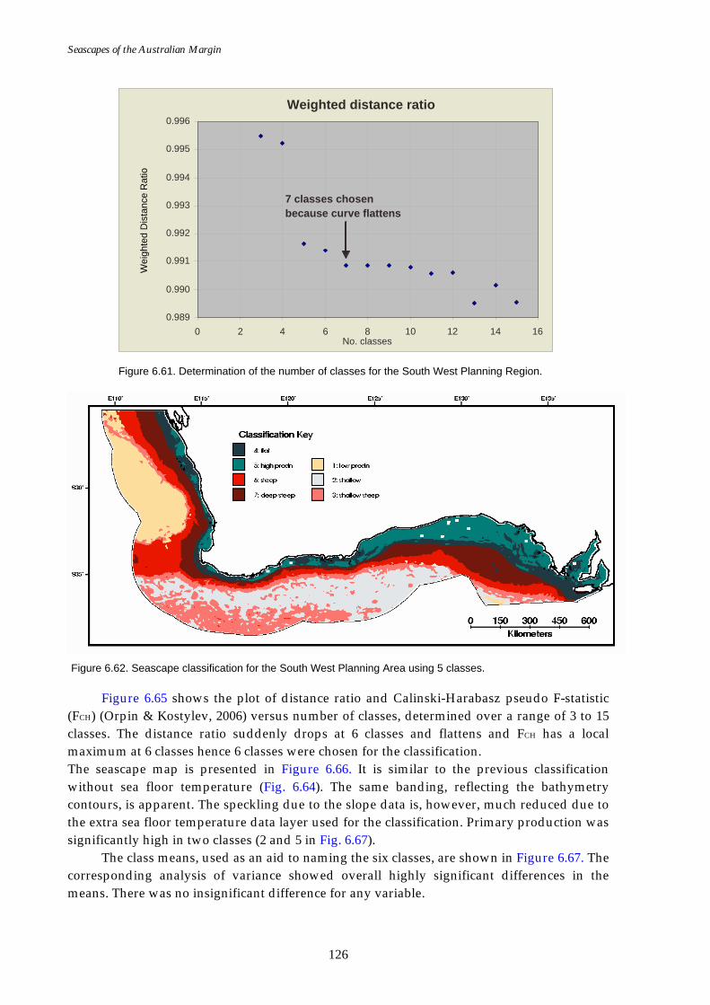
Seascapes of the Australian Margin
126
Figure 6.61. Determination of the number of classes for the South West Planning Region.
Figure 6.62. Seascape classification for the South West Planning Area using 5 classes.
Figure 6.65 shows the plot of distance ratio and Calinski-Harabasz pseudo F-statistic (FCH) (Orpin & Kostylev, 2006) versus number of classes, determined over a range of 3 to 15 classes. The distance ratio suddenly drops at 6 classes and flattens and FCH has a local maximum at 6 classes hence 6 classes were chosen for the classification. The seascape map is presented in Figure 6.66. It is similar to the previous classification without sea floor temperature (Fig. 6.64). The same banding, reflecting the bathymetry contours, is apparent. The speckling due to the slope data is, however, much reduced due to the extra sea floor temperature data layer used for the classification. Primary production was significantly high in two classes (2 and 5 in Fig. 6.67).
The class means, used as an aid to naming the six classes, are shown in Figure 6.67. The corresponding analysis of variance showed overall highly significant differences in the means. There was no insignificant difference for any variable.
Weighted distance ratio
0.989
0.990
0.991
0.992
0.993
0.994
0.995
0.996
0 2 4 6 8 10 12 14 16 No. classes
7 classes chosen because curve flattens
Wei
ghte
d D
ista
nce
Rat
io
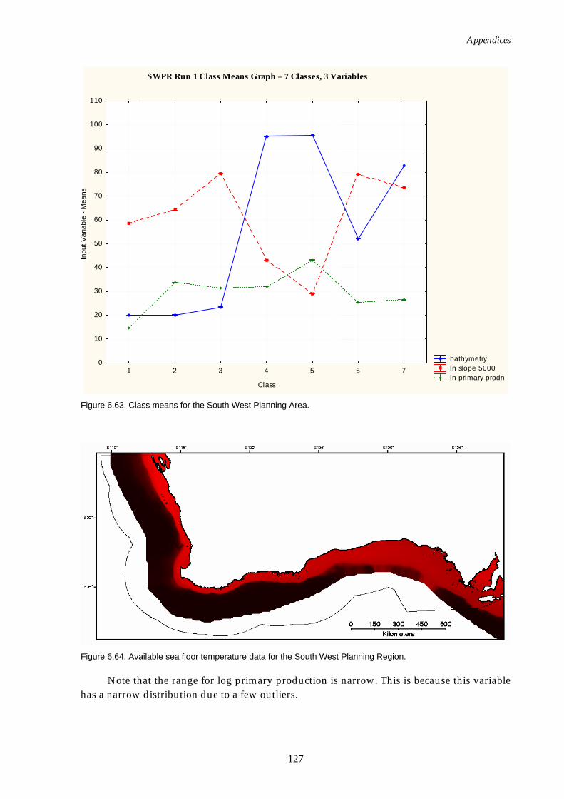
Appendices
127
Southern Planning Area (ED2); Class; LS MeansWilks lambda=.00372, F(18, 2226E3)=7703E2, p=0.0000
bathymetry ln slope 5000 ln primary prodn
1 2 3 4 5 6 7
Class
0
10
20
30
40
50
60
70
80
90
100
110
Figure 6.63. Class means for the South West Planning Area.
Figure 6.64. Available sea floor temperature data for the South West Planning Region.
Note that the range for log primary production is narrow. This is because this variable has a narrow distribution due to a few outliers.
Inpu
t Var
iabl
e - M
eans
SWPR Run 1 Class Means Graph – 7 Classes, 3 Variables
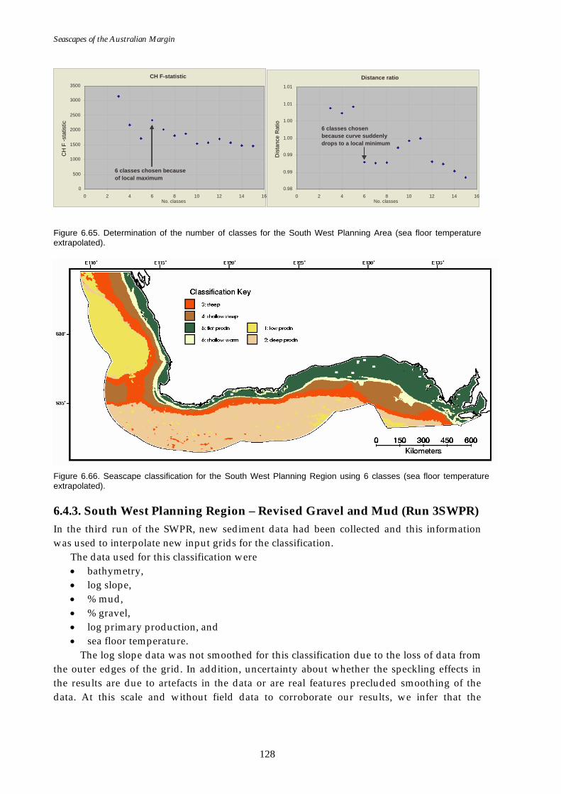
Seascapes of the Australian Margin
128
Figure 6.65. Determination of the number of classes for the South West Planning Area (sea floor temperature extrapolated).
Figure 6.66. Seascape classification for the South West Planning Region using 6 classes (sea floor temperature extrapolated).
6.4.3. South West Planning Region – Revised Gravel and Mud (Run 3SWPR) In the third run of the SWPR, new sediment data had been collected and this information was used to interpolate new input grids for the classification.
The data used for this classification were • bathymetry, • log slope, • % mud, • % gravel, • log primary production, and • sea floor temperature.
The log slope data was not smoothed for this classification due to the loss of data from the outer edges of the grid. In addition, uncertainty about whether the speckling effects in the results are due to artefacts in the data or are real features precluded smoothing of the data. At this scale and without field data to corroborate our results, we infer that the
CH F-statistic
0 500
1000 1500 2000 2500 3000 3500
0 2 4 6 8 10 12 14 16No. classes
6 classes chosen because of local maximum
CH
F -s
tatis
tic
Distance ratio
0.98
0.99
0.99
1.00
1.00
1.01
1.01
0 2 4 6 8 10 12 14 16No. classes
6 classes chosen because curve suddenly drops to a local minimum
Dis
tanc
e R
atio
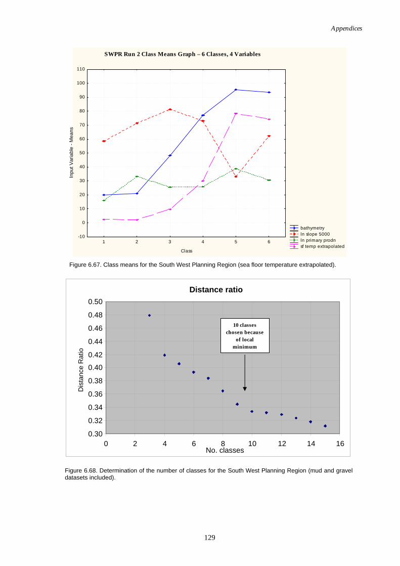
Appendices
129
SWPA (ED2) (sf temp extrapolated) Class; LS MeansWilks lambda=.00286, F(20, 2610E3)=6324E2, p=0.0000
bathymetry ln slope 5000 ln primary prodn sf temp extrapolated
1 2 3 4 5 6
Class
-10
0
10
20
30
40
50
60
70
80
90
100
110
Figure 6.67. Class means for the South West Planning Region (sea floor temperature extrapolated).
Figure 6.68. Determination of the number of classes for the South West Planning Region (mud and gravel datasets included).
Distance ratio
0.30
0.32
0.34
0.36
0.38
0.40
0.42
0.44
0.46
0.48
0.50
0 2 4 6 8 10 12 14 16No. classes
Dis
tanc
e R
atio
10 classes chosen because
of local minimum
Inpu
t Var
iabl
e - M
eans
SWPR Run 2 Class Means Graph – 6 Classes, 4 Variables
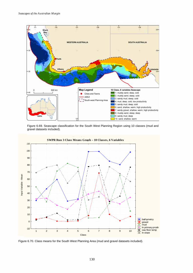
Seascapes of the Australian Margin
130
Figure 6.69. Seascape classification for the South West Planning Region using 10 classes (mud and gravel datasets included).
Class; LS MeansWilks lambda=.00036, F(54, 6751E3)=4682E2, p=0.0000
bathymetry gravel mud ln primary prodn sea floor temp ln slope
1 2 3 4 5 6 7 8 9 10
Class
-10
0
10
20
30
40
50
60
70
80
90
100
110
Figure 6.70. Class means for the South West Planning Area (mud and gravel datasets included).
Inpu
t Var
iabl
e - M
ean
SWPR Run 3 Class Means Graph – 10 Classes, 6 Variables
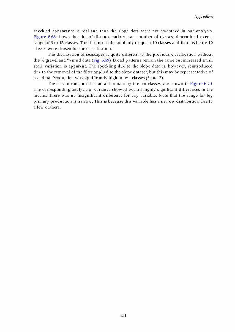
Appendices
131
speckled appearance is real and thus the slope data were not smoothed in our analysis. Figure 6.68 shows the plot of distance ratio versus number of classes, determined over a range of 3 to 15 classes. The distance ratio suddenly drops at 10 classes and flattens hence 10 classes were chosen for the classification.
The distribution of seascapes is quite different to the previous classification without the % gravel and % mud data (Fig. 6.69). Broad patterns remain the same but increased small scale variation is apparent. The speckling due to the slope data is, however, reintroduced due to the removal of the filter applied to the slope dataset, but this may be representative of real data. Production was significantly high in two classes (6 and 7).
The class means, used as an aid to naming the ten classes, are shown in Figure 6.70. The corresponding analysis of variance showed overall highly significant differences in the means. There was no insignificant difference for any variable. Note that the range for log primary production is narrow. This is because this variable has a narrow distribution due to a few outliers.

Seascapes of the Australian Margin
132
6.5 APPENDIX E – FUZZY CLUSTER VALIDITY MEASURES
6.5.1. Bezdek's PC and PE Indices These are two fuzzy cluster validity measures, partition co-efficient (PC) and partition entropy (PE) that can be applied for any fuzzy cluster. These indexes are defined as:
(Eq. 6.15)
and;
(Eq. 6.16)
where µij is the fuzzy c-partition, {a1…ac} is the set of c cluster centres and n is number of grid cells with values (does not include ‘no data’; i.e., 9999). For more information on this index refer to Pal and Bezdek (1995). PC takes the maximum value and PE assumes the minimum value on the hard c-partition.
6.5.2. Fuzzy Hyper Volume The fuzzy hyper volume (FHV) validity index, proposed by Gath and Geva (1989) is defined by:
(Eq. 6.17)
where;
(Eq. 6.18)
The matrix Fi denotes the fuzzy covariance matrix of cluster i and m is the fuzzy exponent (the overlap parameter). A fuzzy partition can be expected to have a low FHV(c) value if the partition is tight. Thus an optimal c is indicated by the minimum FHV (Wu & Yang, 2005). For more information see Gath and Geva (1989).
6.5.3. Xie-Beni (XBm) Index This index developed by Xie and Beni is defined as:
(Eq. 6.19)
Using the XBm the optimal number of clusters can be obtained by minimizing the index value. For more information see Xie and Beni (1991).
6.5.4. PBMF Index This recently developed (2005) index was developed for both crisp and fuzzy clustering. This algorithm was developed from the PBM-index. The fuzzy index is obtained by incorporating fuzzy distances. It is defined as follows:
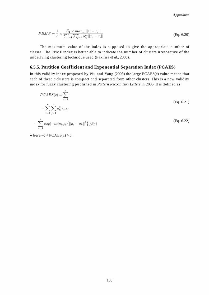
Appendices
133
(Eq. 6.20)
The maximum value of the index is supposed to give the appropriate number of classes. The PBMF index is better able to indicate the number of clusters irrespective of the underlying clustering technique used (Pakhira et al., 2005).
6.5.5. Partition Coefficient and Exponential Separation Index (PCAES) In this validity index proposed by Wu and Yang (2005) the large PCAES(c) value means that each of these c clusters is compact and separated from other clusters. This is a new validity index for fuzzy clustering published in Pattern Recognition Letters in 2005. It is defined as:
(Eq. 6.21)
(Eq. 6.22)
where –c < PCAES(c) > c.