Geoscience Australia Record 2004/18

Airborne Gravity 2004 Abstracts from the ASEG-PESA Airborne Gravity 2004 Workshop Edited by Richard Lane

Department of Industry, Tourism & Resources Minister for Industry, Tourism & Resources: The Hon. Ian Macfarlane, MP Parliamentary Secretary: The Hon. Warren Entsch, MP Secretary: Mark Paterson Geoscience Australia Chief Executive Officer: Neil Williams © Commonwealth of Australia 2004 This work is copyright. Apart from any fair dealings for the purposes of study, research, criticism or review, as permitted under the Copyright Act, no part may be reproduced by any process without written permission. Inquiries should be directed to the Communications Unit, Geoscience Australia, GPO Box 378, Canberra City, ACT, 2601 ISSN: 1448-2177 ISBN: 1 920871 13 6 GeoCat no. 61129 Bibliographic Reference: a) For the entire publication Lane, R.J.L., editor, 2004, Airborne Gravity 2004 – Abstracts from the ASEG-PESA Airborne Gravity 2004 Workshop: Geoscience Australia Record 2004/18. b) For an individual paper van Kann, F., 2004, Requirements and general principles of airborne gravity gradiometers for mineral exploration, in R.J.L. Lane, editor, Airborne Gravity 2004 - Abstracts from the ASEG-PESA Airborne Gravity 2004 Workshop: Geoscience Australia Record 2004/18, 1-5. Geoscience Australia has tried to make the information in this product as accurate as possible. However, it does not guarantee that the information is totally accurate or complete. THEREFORE, YOU SHOULD NOT RELY SOLELY ON THIS INFORMATION WHEN MAKING A COMMERCIAL DECISION.

ii

Contents “Airborne Gravity 2004 Workshop” Record R.J.L. Lane, M.H. Dransfield, D. Robson, R.J. Smith and G. Walker…………………………………..v Requirements and general principles of airborne gravity gradiometers for mineral exploration F. van Kann…………………………………………………………………………………………………...1 The Air-FTG™ airborne gravity gradiometer system C.A. Murphy…………………………………………………………………………………………………..7 The FALCON® airborne gravity gradiometer systems M.H. Dransfield and J.B. Lee……………………………………………………………………………...15 A superconducting gravity gradiometer tool for exploration J.M. Lumley, J.P. White, G. Barnes, D. Huang and H.J. Paik…………………………………………21 A high resolution airborne gravimeter and airborne gravity gradiometer B. Tryggvason, B. Main and B. French…………………………………………………………………..41 The AIRGrav airborne gravity system S. Sander, M. Argyle, S. Elieff, S. Ferguson, V. Lavoie and L. Sander………………………………49 The GT-1A mobile gravimeter A. Gabell, H. Tuckett and D. Olson……………………………………………………………………….55 A synopsis of airborne gravity data presentation, modelling, interpretation and inversion software G. Walker……………………………………………………………………………………………………63 Acquisition and preliminary impressions of airborne gravity gradient and aeromagnetic data in the Eastern Papuan Basin, Papua New Guinea A. Nelson…………………………………………………………………………………………………….65 Evaluation of a full tensor gravity gradiometer for kimberlite exploration D. Hatch……………………………………………………………………………………………………..73 Integrating ground and airborne data into regional gravity compilations R.J.L. Lane…………………………………………………………………………………………………..81 Airborne gravity data acquisition and processing: A case study in the Prince Charles Mountains, East Antarctica M. McLean, D. Damaske, V. Damm and G. Reitmayr………………………………………………….99 AIRGrav airborne gravity survey in Timmins, Ontario S. Elieff and S. Sander……………………………………………………………………………………111 Examples of FALCON™ data from diamond exploration projects in Northern Australian D. Isles and I. Moody……………………………………………………………………………………..121 A comparison of the Falcon® and Air-FTG™ airborne gravity gradiometer systems at the Kokong Test Block, Botswana D. Hinks, S. McIntosh and R.J.L. Lane…………………………………………………………………125 Analysis of errors in gravity derived from the Falcon® Airborne Gravity Gradiometer D.B. Boggs and M.H. Dransfield………………………………………………………………………...135

iii

“Airborne Gravity 2004 Workshop” Record Richard Lane Geoscience Australia richard.lane@ga.gov.au Mark Dransfield BHP Billiton Mark.H.Dransfield@bhpbilliton.com David Robson NSW Department of Primary Industry – Minerals david.robson@minerals.nsw.gov.au Robert Smith Greenfields Geophysics greengeo@bigpond.net.au Greg Walker BHP Billiton Greg.B.Walker@BHPBilliton.com

Preface The "Airborne Gravity 2004 Workshop" was held in Sydney on August 15, in conjunction with ASEG-PESA Sydney 2004 (the ASEG's 17th Geophysical Conference and Exhibition). The aims of the workshop were to provide participants with a review of the current state of the art in airborne gravity instrumentation, to present case histories of the use of these methods in minerals and petroleum applications, and to distribute sample data sets. "Airborne gravity" is used in this context to include both airborne gravimeter and airborne gravity gradiometer methods. The program was split into 2 sessions. The morning session provided a review of the systems, with presentations covering a number of systems currently in operation as well as some that are still under development. The focus shifted in the afternoon session to case histories, with examples from surveys spanning the globe; from Antarctica to the tropics of Papua New Guinea, from Africa through Australia to Canada. To capture the essence of the day and to promote the ongoing development of airborne geophysical methods, speakers were invited to submit papers for inclusion in a workshop volume. The papers were reviewed prior to publication in this Geoscience Australia Record. Participants received a copy at the workshop, and additional copies of the Record are available on an ongoing basis from Geoscience Australia (www.ga.gov.au).

Units Physical quantities should be expressed in SI units. The Bureau International des Poids et Mesures (BIPM) is the custodian of this system. To quote from their website (www.bipm.fr): “Its mandate is to provide the basis for a single, coherent system of measurements throughout the world, traceable to the International System of Units (SI)”. The SI unit for acceleration is “metre per second squared” (m/s2). The signals encountered in gravity surveys for exploration are small, and the prefix “micro” is commonly used (micrometre per second squared, µm/s2). The gal (or Gal), equal to 1 cm/s2, is a derived unit for acceleration in the CGS system of units. A prefix of “milli” is commonly used (milligal, mGal). In rare cases in the literature, a “gravity unit” (gu) may be encountered. In this publication, the µm/s2 has been the preferred unit for gravity measurements, but mGal has been accepted. 1 µm/s2 = 10-6 m/s2

1 mGal = 10 µm/s2

1 gu = 1 µm/s2 The gravity gradient is a gradient of acceleration and so the appropriate units are acceleration units divided by distance units. Thus, “per second squared” (s-2) is appropriate in the SI system. Typical gravity gradients measured in exploration are extremely small, and the prefix “nano” is appropriate in most circumstances (per

v

nanosecond squared, ns-2). The eotvos unit (Eo), although not recognised in either the SI or CGS systems, is used almost universally in geophysics as the unit for gravity gradient measurements. It is equal to 1 ns-2. In this publication, the ns-2 and Eo have both been accepted as units for gravity gradient measurements. 1 ns-2 = 10-9 s-2

1 Eo= 1 ns-2

Acknowledgments The Airborne Gravity 2004 Workshop Organising Committee would like to acknowledge the support of the ASEG-PESA 2004 Conference Organizing Committee and the Conference Secretariat. Support from Geoscience Australia, BHP Billiton and the NSW Department of Primary Industries - Mineral Resources helped to make the workshop a success. The diligence of Mario Bacchin, Katharine Hagan, Angie Jaensch, Jim Mason, Peter Milligan, Ian Hone and Roger Clifton enabled this Record to be produced in time for the Workshop, despite a tight deadline. Finally, a vote of thanks goes to the speakers who committed their time and energy to deliver presentations on the day and to compose this permanent record of the event.

vi

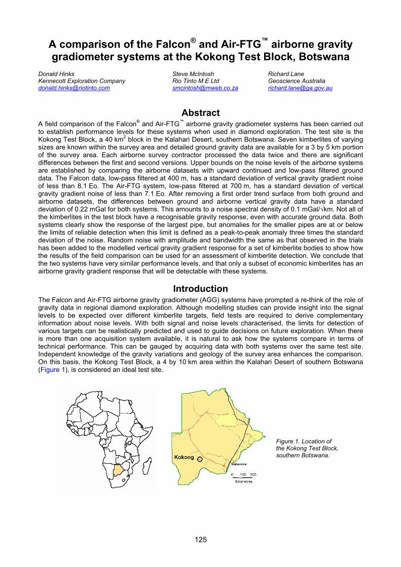
A comparison of the Falcon® and Air-FTG™ airborne gravity gradiometer systems at the Kokong Test Block, Botswana

Donald Hinks Steve McIntosh Richard Lane Kennecott Exploration Company Rio Tinto M E Ltd Geoscience Australia donald.hinks@riotinto.com smcintosh@mweb.co.za richard.lane@ga.gov.au

Abstract A field comparison of the Falcon® and Air-FTG™ airborne gravity gradiometer systems has been carried out to establish performance levels for these systems when used in diamond exploration. The test site is the Kokong Test Block, a 40 km2 block in the Kalahari Desert, southern Botswana. Seven kimberlites of varying sizes are known within the survey area and detailed ground gravity data are available for a 3 by 5 km portion of the survey area. Each airborne survey contractor processed the data twice and there are significant differences between the first and second versions. Upper bounds on the noise levels of the airborne systems are established by comparing the airborne datasets with upward continued and low-pass filtered ground data. The Falcon data, low-pass filtered at 400 m, has a standard deviation of vertical gravity gradient noise of less than 8.1 Eo. The Air-FTG system, low-pass filtered at 700 m, has a standard deviation of vertical gravity gradient noise of less than 7.1 Eo. After removing a first order trend surface from both ground and airborne datasets, the differences between ground and airborne vertical gravity data have a standard deviation of 0.22 mGal for both systems. This amounts to a noise spectral density of 0.1 mGal/√km. Not all of the kimberlites in the test block have a recognisable gravity response, even with accurate ground data. Both systems clearly show the response of the largest pipe, but anomalies for the smaller pipes are at or below the limits of reliable detection when this limit is defined as a peak-to-peak anomaly three times the standard deviation of the noise. Random noise with amplitude and bandwidth the same as that observed in the trials has been added to the modelled vertical gravity gradient response for a set of kimberlite bodies to show how the results of the field comparison can be used for an assessment of kimberlite detection. We conclude that the two systems have very similar performance levels, and that only a subset of economic kimberlites has an airborne gravity gradient response that will be detectable with these systems.

Introduction The Falcon and Air-FTG airborne gravity gradiometer (AGG) systems have prompted a re-think of the role of gravity data in regional diamond exploration. Although modelling studies can provide insight into the signal levels to be expected over different kimberlite targets, field tests are required to derive complementary information about noise levels. With both signal and noise levels characterised, the limits for detection of various targets can be realistically predicted and used to guide decisions on future exploration. When there is more than one acquisition system available, it is natural to ask how the systems compare in terms of technical performance. This can be gauged by acquiring data with both systems over the same test site. Independent knowledge of the gravity variations and geology of the survey area enhances the comparison. On this basis, the Kokong Test Block, a 4 by 10 km area within the Kalahari Desert of southern Botswana (Figure 1), is considered an ideal test site.

Figure 1. Location of the Kokong Test Block, southern Botswana.

125

The area was explored between 1979 and 1985 by Falconbridge, who discovered a total of seven kimberlite pipes using airborne magnetics, ground gravity and indicator sampling. The locations of the kimberlites discovered during this period are shown superimposed on a Total Magnetic Intensity image in Figure 2. The pipes are buried beneath 70 to 120 m of Kalahari Sand and the present ground surface is flat. Detailed ground gravity data are available for a portion of the survey area. The pipes have a variety of gravity responses, reflecting differences in diameter, density contrast and surrounding host lithology. Table 1 summarises basic information for these kimberlites. The diameter values were estimated from magnetic and gravity data as there is insufficient drilling of these sub-economic pipes to determine their size directly.

Figure 2. Airborne Total Magnetic Intensity data for the Kokong Test Block, showing the locations of kimberlites known prior to the airborne gravity gradiometer surveys. The magnetic and gravity responses of these pipes do not always coincide; KS40 has an offset magnetic high and gravity low, and the drill hole which intersected KS31 was drilled between a magnetic low and gravity low. KS66 does not have a magnetic anomaly at all and KS67 is associated with a magnetic low. The ground gravity anomalies for all these pipes are either lows or below the detection level of 0.1 mGal. The gravity features vary in amplitude from less than -0.1 mGal to more than -1.2 mGal in the case of the largest body, KS40. The pipe diameters were estimated from ground geophysical data, and range from 300 m (KS31) to 1000 m (KS40).

Table 1. Diameter, thickness of cover and gravity anomaly characteristics of the kimberlites in the Kokong Test Block.

Kimberlite Diameter Thickness of Kalahari Sand cover

Amplitude of associated ground gravity anomaly

(m) (m) (mGal) KS40 1000 120 -1.20 KS67 400 77 -0.40 KS66 600 105 -0.30 KS31 300 80 -0.25 KS34 500 70 -0.15 KS11 600 90 <0.10 KS10 600 99 <0.10

126

Airborne gravity gradiometer surveys The Falcon and Air-FTG systems are described in greater detail elsewhere in this volume and will only be briefly summarised here. The systems both use Lockheed-Martin AGG technology to measure acceleration. The Falcon system measures two horizontal gravity gradients which can be spatially transformed to produce vertical gravity (gZ) and vertical gravity gradient (Gzz) data. The Air-FTG system is a full tensor gravity gradient system which can measure the five independent gravity gradient tensor components. Transformation to vertical gravity again requires spatial transformation. A direct comparison of system performance levels based on surveys over the same area under the same conditions provides the evidence required to judge the relative technical merits of the systems involved. Although the two surveys were flown a year apart (the Falcon survey in January 2002 and the Air-FTG survey in January 2003), similar elevated levels of turbulence were encountered during both surveys. January is not the ideal month to acquire airborne gravity gradiometer data as air turbulence from the summer heat is at a maximum at this time of year. Both contractors processed their data twice, and in each case, there are significant differences between the first and second versions. This is likely to be due to a combination of factors, including the low level of geological signal in the test area, the amount of noise present in the airborne datasets, the small signal from the buried kimberlite pipes, and the relative immaturity of the data processing techniques. Only the final results are presented here.

Falcon Survey The Falcon data were acquired over two flights, with 100 m line spacing, terrain clearance of 80 m, and east-west line direction. North-south tie lines were spaced at 2500 m intervals. An initial gZ and Gzz dataset was provided and later, a second dataset was provided which was produced with new processing routines. Although terrain corrections were produced, they were not applied as the maximum terrain correction value of less than 0.7 Eo was considered unimportant. During assessment of the data, amplitude spectra have been calculated for each row in the final Gzz grid and then averaged (Figure 3). The rapid drop in amplitude for wavelengths less than 400 m indicates that a high order (i.e., steep) low-pass filter with a 400 m cut-off was applied to these data.

Air FTG Survey This was the second survey flown with the Air-FTG system in Africa, and it would be natural to expect that improvements to acquisition and processing methods would be made as greater experience was gained. The Kokong survey involved eight flights, with 100 m line spacing, terrain clearance of 90 m, and east-west line direction. Due to turbulence and concerns over data quality, the spacing of north-south tie lines was reduced to 250 m and a number of the flight lines were re-flown. Two versions of the gZ and Gzz data were supplied. The dynamic range of the data in the first set of products is much higher than in the second version, which is interpreted as an indication that considerably more noise is present in the first set of products or that more filtering was applied the second time around. The first version of the Gzz grid has a standard deviation of 17 Eo, whilst the final version has a standard deviation of 7.1 Eo. For comparison, the standard deviation of the Falcon final Gzz grid is 8.7 Eo. As far as we are aware, the complete Air-FTG dataset including original and re-flown lines was used for the preliminary processing. It is unclear whether noisy flight lines were excluded when compiling the final products. No terrain corrections were calculated for the Air-FTG data. The experience from the Falcon survey suggests that the effect of this omission is not significant. Whilst analysing the data, an average amplitude spectrum from the rows of the final Gzz grid has been derived (Figure 3). The drop in amplitude at the short wavelength end of the spectrum is less dramatic for the Air-FTG Gzz data. It was inferred through comparison with the spectrum for the Falcon Gzz data that a gradational, low order low-pass filter was applied to wavelengths less than 700 m.

127

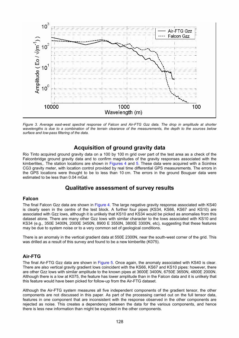
Figure 3. Average east-west spectral response of Falcon and Air-FTG Gzz data. The drop in amplitude at shorter wavelengths is due to a combination of the terrain clearance of the measurements, the depth to the sources below surface and low-pass filtering of the data.

Acquisition of ground gravity data Rio Tinto acquired ground gravity data on a 100 by 100 m grid over part of the test area as a check of the Falconbridge ground gravity data and to confirm magnitudes of the gravity responses associated with the kimberlites,. The station locations are shown in Figures 4 and 5. These data were acquired with a Scintrex CG3 gravity meter, with location control provided by real time differential GPS measurements. The errors in the GPS locations were thought to be to less than 10 cm. The errors in the ground Bouguer data were estimated to be less than 0.04 mGal.

Qualitative assessment of survey results

Falcon The final Falcon Gzz data are shown in Figure 4. The large negative gravity response associated with KS40 is clearly seen in the centre of the test block. A further four pipes (KS34, KS66, KS67 and KS10) are associated with Gzz lows, although it is unlikely that KS10 and KS34 would be picked as anomalies from this dataset alone. There are many other Gzz lows with similar character to the lows associated with KS10 and KS34 (e.g., 350E 3400N, 2000E 3450N, 8900 E 3550N, 3800E 3300N, etc), suggesting that these features may be due to system noise or to a very common set of geological conditions. There is an anomaly in the vertical gradient data at 550E 2300N, near the south-west corner of the grid. This was drilled as a result of this survey and found to be a new kimberlite (K075).

Air-FTG The final Air-FTG Gzz data are shown in Figure 5. Once again, the anomaly associated with KS40 is clear. There are also vertical gravity gradient lows coincident with the KS66, KS67 and KS10 pipes: however, there are other Gzz lows with similar amplitude to the known pipes at 3600E 3400N, 6750E 3650N, 4800E 2000N. Although there is a low at K075, the feature has lower amplitude than in the Falcon data and it is unlikely that this feature would have been picked for follow-up from the Air-FTG dataset. Although the Air-FTG system measures all five independent components of the gradient tensor, the other components are not discussed in this paper. As part of the processing carried out on the full tensor data, features in one component that are inconsistent with the response observed in the other components are rejected as noise. This creates a dependency between the data for the various components, and hence there is less new information than might be expected in the other components.

128

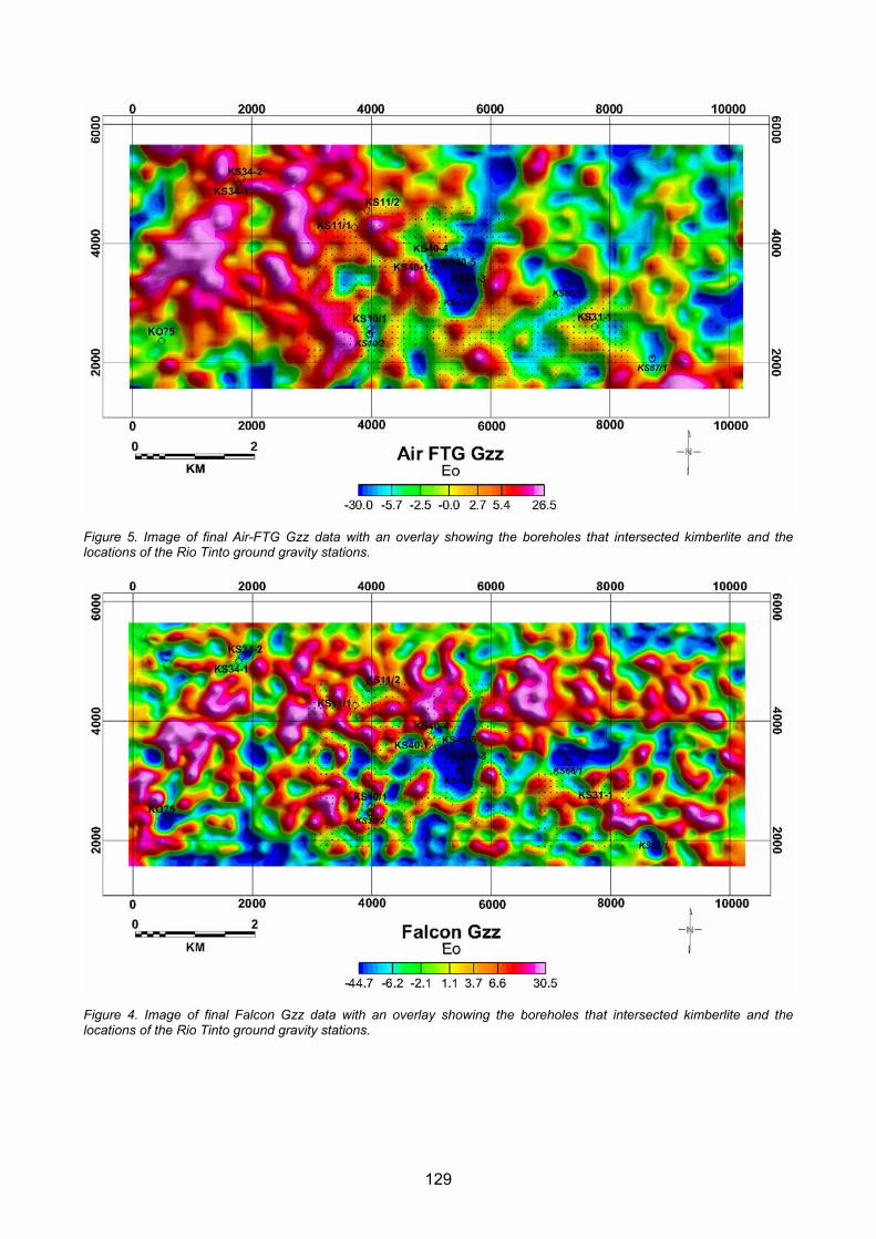
Figure 5. Image of final Air-FTG Gzz data with an overlay showing the boreholes that intersected kimberlite and the locations of the Rio Tinto ground gravity stations.

Figure 4. Image of final Falcon Gzz data with an overlay showing the boreholes that intersected kimberlite and the locations of the Rio Tinto ground gravity stations.

129

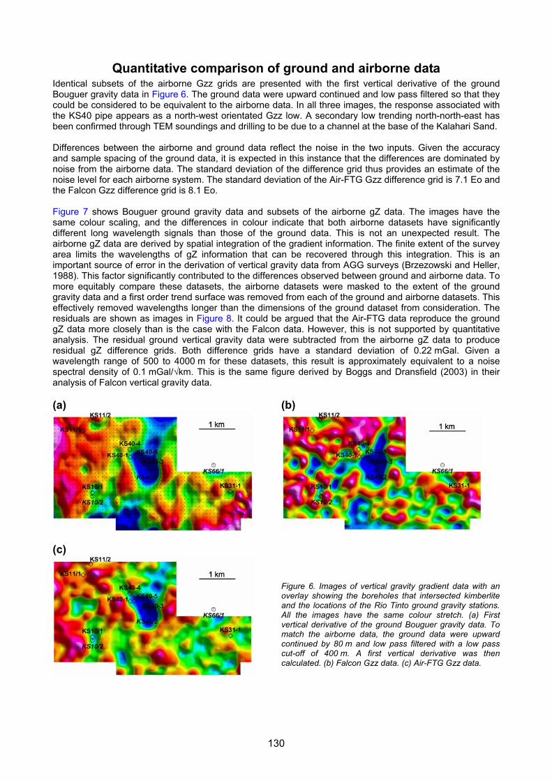
Quantitative comparison of ground and airborne data Identical subsets of the airborne Gzz grids are presented with the first vertical derivative of the ground Bouguer gravity data in Figure 6. The ground data were upward continued and low pass filtered so that they could be considered to be equivalent to the airborne data. In all three images, the response associated with the KS40 pipe appears as a north-west orientated Gzz low. A secondary low trending north-north-east has been confirmed through TEM soundings and drilling to be due to a channel at the base of the Kalahari Sand. Differences between the airborne and ground data reflect the noise in the two inputs. Given the accuracy and sample spacing of the ground data, it is expected in this instance that the differences are dominated by noise from the airborne data. The standard deviation of the difference grid thus provides an estimate of the noise level for each airborne system. The standard deviation of the Air-FTG Gzz difference grid is 7.1 Eo and the Falcon Gzz difference grid is 8.1 Eo. Figure 7 shows Bouguer ground gravity data and subsets of the airborne gZ data. The images have the same colour scaling, and the differences in colour indicate that both airborne datasets have significantly different long wavelength signals than those of the ground data. This is not an unexpected result. The airborne gZ data are derived by spatial integration of the gradient information. The finite extent of the survey area limits the wavelengths of gZ information that can be recovered through this integration. This is an important source of error in the derivation of vertical gravity data from AGG surveys (Brzezowski and Heller, 1988). This factor significantly contributed to the differences observed between ground and airborne data. To more equitably compare these datasets, the airborne datasets were masked to the extent of the ground gravity data and a first order trend surface was removed from each of the ground and airborne datasets. This effectively removed wavelengths longer than the dimensions of the ground dataset from consideration. The residuals are shown as images in Figure 8. It could be argued that the Air-FTG data reproduce the ground gZ data more closely than is the case with the Falcon data. However, this is not supported by quantitative analysis. The residual ground vertical gravity data were subtracted from the airborne gZ data to produce residual gZ difference grids. Both difference grids have a standard deviation of 0.22 mGal. Given a wavelength range of 500 to 4000 m for these datasets, this result is approximately equivalent to a noise spectral density of 0.1 mGal/√km. This is the same figure derived by Boggs and Dransfield (2003) in their analysis of Falcon vertical gravity data. (a)

(b)

(c)

Figure 6. Images of vertical gravity gradient data with an overlay showing the boreholes that intersected kimberlite and the locations of the Rio Tinto ground gravity stations. All the images have the same colour stretch. (a) First vertical derivative of the ground Bouguer gravity data. To match the airborne data, the ground data were upward continued by 80 m and low pass filtered with a low pass cut-off of 400 m. A first vertical derivative was then calculated. (b) Falcon Gzz data. (c) Air-FTG Gzz data.

130

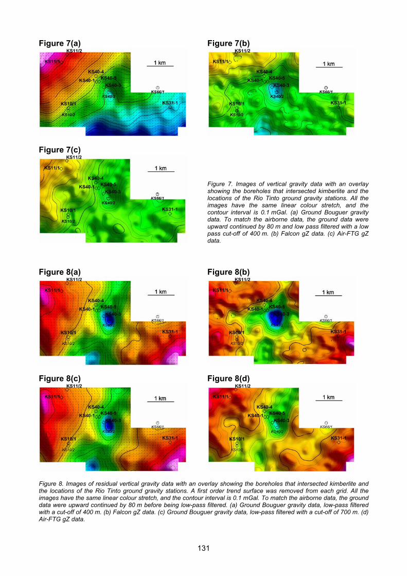
Figure 7(a)

Figure 7(b)

Figure 7(c)

Figure 7. Images of vertical gravity data with an overlay showing the boreholes that intersected kimberlite and the locations of the Rio Tinto ground gravity stations. All the images have the same linear colour stretch, and the contour interval is 0.1 mGal. (a) Ground Bouguer gravity data. To match the airborne data, the ground data were upward continued by 80 m and low pass filtered with a low pass cut-off of 400 m. (b) Falcon gZ data. (c) Air-FTG gZ data.

Figure 8(a)

Figure 8(b)

Figure 8(c)

Figure 8(d)

Figure 8. Images of residual vertical gravity data with an overlay showing the boreholes that intersected kimberlite and the locations of the Rio Tinto ground gravity stations. A first order trend surface was removed from each grid. All the images have the same linear colour stretch, and the contour interval is 0.1 mGal. To match the airborne data, the ground data were upward continued by 80 m before being low-pass filtered. (a) Ground Bouguer gravity data, low-pass filtered with a cut-off of 400 m. (b) Falcon gZ data. (c) Ground Bouguer gravity data, low-pass filtered with a cut-off of 700 m. (d) Air-FTG gZ data.

131

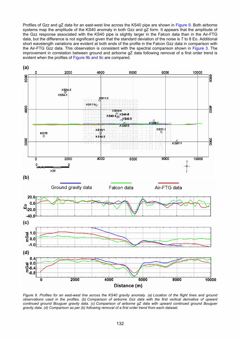
Profiles of Gzz and gZ data for an east-west line across the KS40 pipe are shown in Figure 9. Both airborne systems map the amplitude of the KS40 anomaly in both Gzz and gZ form. It appears that the amplitude of the Gzz response associated with the KS40 pipe is slightly larger in the Falcon data than in the Air-FTG data, but the difference is not significant given that the standard deviation of the noise is 7 to 8 Eo. Additional short wavelength variations are evident at both ends of the profile in the Falcon Gzz data in comparison with the Air-FTG Gzz data. This observation is consistent with the spectral comparison shown in Figure 3. The improvement in correlation between ground and airborne gZ data following removal of a first order trend is evident when the profiles of Figure 9b and 9c are compared. (a)

(b)

(c)

(d)

Figure 9. Profiles for an east-west line across the KS40 gravity anomaly. (a) Location of the flight lines and ground observations used in the profiles. (b) Comparison of airborne Gzz data with the first vertical derivative of upward continued ground Bouguer gravity data. (c) Comparison of airborne gZ data with upward continued ground Bouguer gravity data. (d) Comparison as per (b) following removal of a first order trend from each dataset.

132

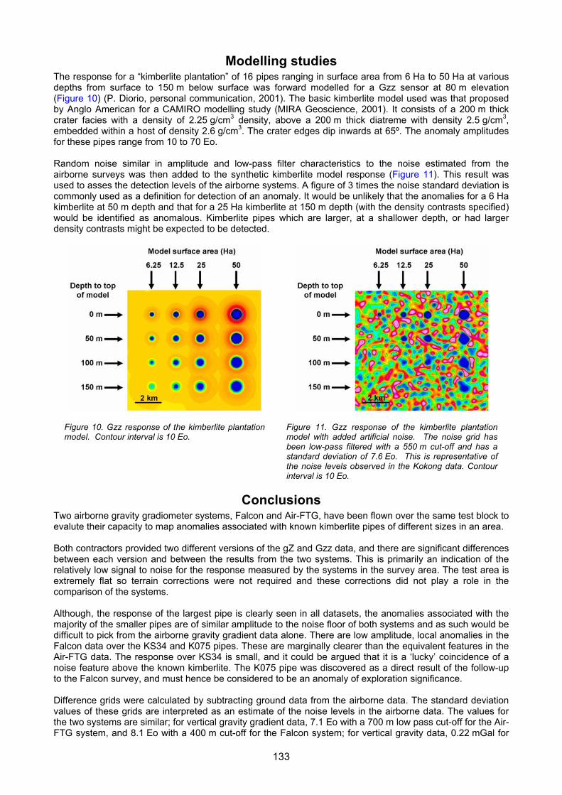
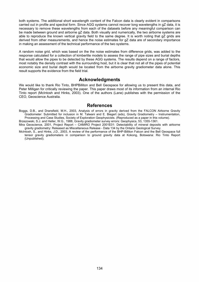
Modelling studies The response for a “kimberlite plantation” of 16 pipes ranging in surface area from 6 Ha to 50 Ha at various depths from surface to 150 m below surface was forward modelled for a Gzz sensor at 80 m elevation (Figure 10) (P. Diorio, personal communication, 2001). The basic kimberlite model used was that proposed by Anglo American for a CAMIRO modelling study (MIRA Geoscience, 2001). It consists of a 200 m thick crater facies with a density of 2.25 g/cm3 density, above a 200 m thick diatreme with density 2.5 g/cm3, embedded within a host of density 2.6 g/cm3. The crater edges dip inwards at 65º. The anomaly amplitudes for these pipes range from 10 to 70 Eo. Random noise similar in amplitude and low-pass filter characteristics to the noise estimated from the airborne surveys was then added to the synthetic kimberlite model response (Figure 11). This result was used to asses the detection levels of the airborne systems. A figure of 3 times the noise standard deviation is commonly used as a definition for detection of an anomaly. It would be unlikely that the anomalies for a 6 Ha kimberlite at 50 m depth and that for a 25 Ha kimberlite at 150 m depth (with the density contrasts specified) would be identified as anomalous. Kimberlite pipes which are larger, at a shallower depth, or had larger density contrasts might be expected to be detected.

Figure 10. Gzz response of the kimberlite plantation model. Contour interval is 10 Eo.

Figure 11. Gzz response of the kimberlite plantation model with added artificial noise. The noise grid has been low-pass filtered with a 550 m cut-off and has a standard deviation of 7.6 Eo. This is representative of the noise levels observed in the Kokong data. Contour interval is 10 Eo.

Conclusions Two airborne gravity gradiometer systems, Falcon and Air-FTG, have been flown over the same test block to evalute their capacity to map anomalies associated with known kimberlite pipes of different sizes in an area. Both contractors provided two different versions of the gZ and Gzz data, and there are significant differences between each version and between the results from the two systems. This is primarily an indication of the relatively low signal to noise for the response measured by the systems in the survey area. The test area is extremely flat so terrain corrections were not required and these corrections did not play a role in the comparison of the systems. Although, the response of the largest pipe is clearly seen in all datasets, the anomalies associated with the majority of the smaller pipes are of similar amplitude to the noise floor of both systems and as such would be difficult to pick from the airborne gravity gradient data alone. There are low amplitude, local anomalies in the Falcon data over the KS34 and K075 pipes. These are marginally clearer than the equivalent features in the Air-FTG data. The response over KS34 is small, and it could be argued that it is a ‘lucky’ coincidence of a noise feature above the known kimberlite. The K075 pipe was discovered as a direct result of the follow-up to the Falcon survey, and must hence be considered to be an anomaly of exploration significance. Difference grids were calculated by subtracting ground data from the airborne data. The standard deviation values of these grids are interpreted as an estimate of the noise levels in the airborne data. The values for the two systems are similar; for vertical gravity gradient data, 7.1 Eo with a 700 m low pass cut-off for the Air-FTG system, and 8.1 Eo with a 400 m cut-off for the Falcon system; for vertical gravity data, 0.22 mGal for

133

134

both systems. The additional short wavelength content of the Falcon data is clearly evident in comparisons carried out in profile and spectral form. Since AGG systems cannot recover long wavelengths in gZ data, it is necessary to remove these wavelengths from each of the datasets before any meaningful comparison can be made between ground and airborne gZ data. Both visually and numerically, the two airborne systems are able to reproduce the known vertical gravity field to the same degree. It is worth noting that gZ grids are derived from other measurements, and hence the noise estimates for gZ data are of secondary importance in making an assessment of the technical performance of the two systems. A random noise grid, which was based on the the noise estimates from difference grids, was added to the response calculated for a collection of kimberlite models to assess the range of pipe sizes and burial depths that would allow the pipes to be detected by these AGG systems. The results depend on a range of factors, most notably the density contrast with the surrounding host, but it is clear that not all of the pipes of potential economic size and burial depth would be located from the airborne gravity gradiometer data alone. This result supports the evidence from the field trial.

Acknowledgments We would like to thank Rio Tinto, BHPBilliton and Bell Geospace for allowing us to present this data, and Peter Milligan for critically reviewing the paper. This paper draws most of its information from an internal Rio Tinto report (McIntosh and Hinks, 2003). One of the authors (Lane) publishes with the permission of the CEO, Geoscience Australia.

References Boggs, D.B., and Dransfield, M.H., 2003, Analysis of errors in gravity derived from the FALCON Airborne Gravity

Gradiometer: Submitted for inclusion in M. Talwani and E. Biegert (eds), Gravity Gradiometry – Instrumentation, Processing and Case Studies, Society of Exploration Geophysicists. (Reproduced as a paper in this volume).

Brzezowski, S.J. and Heller, W.G., 1988, Gravity gradiometer survey errors: Geophysics, 53, 1355-1361. Mira Geoscience, 2001, Project Report – CAMIRO Project 2001E01: Detectability of mineral deposits with airborne

gravity gradiometry: Released as Miscellaneous Release - Data 134 by the Ontario Geological Survey. McIntosh, S., and Hinks, J.D., 2003, A review of the performance of the BHP-Billiton Falcon and the Bell Geospace full

tensor gravity gradiometers in comparison to ground gravity data at Kokong, Botswana: Rio Tinto Report (Unpublished).