geometric quantum mechanics - arxiv.org · from a modern perspective the current ﬂows in reverse,...

arX

iv:q

uant

-ph/

9906

086v

2 1

5 O

ct 1

999

Geometric Quantum Mechanics

By Dorje C. Brody1 and Lane P. Hughston2

1Blackett Laboratory, Imperial College, London SW7 2BZ, UKand DAMTP, Silver Street, Cambridge CB3 9EW, UK2Department of Mathematics, King’s College London,

Strand, London WC2R 2LS, UK

The manifold of pure quantum states can be regarded as a complex projectivespace endowed with the unitary-invariant Riemannian geometry of Fubini andStudy. According to the principles of geometric quantum mechanics, the detailedphysical characteristics of a given quantum system can be represented by specificgeometrical features that are selected and preferentially identified in this complexmanifold. In particular, any specific feature of projective geometry gives rise toa physically realisable characteristic in quantum mechanics. Here we construct anumber of examples of such geometrical features as they arise in the state spacesfor spin-1

2 , spin-1, and spin-32 systems, and for pairs of spin-1

2 systems. A study isundertaken on the geometry of entangled states, and a natural measure is assignedto the degree of entanglement of a given state for a general multi-particle system.The properties of this measure are analysed in detail for the entangled states of apair of spin-1

2 particles, thus enabling us to determine the structure of the spaceof maximally entangled states. With the specification of a quantum Hamiltonian,the resulting Schrodinger trajectories induce an isometry of the Fubini-Studymanifold. For a generic quantum evolution, the corresponding Killing trajectoryis quasiergodic on a toroidal subspace of the energy surface. When the dynamicaltrajectory is lifted orthogonally to Hilbert space, it induces a geometric phaseshift on the wave function. The uncertainty of an observable in a given stateis the length of the gradient vector of the level surface of the expectation of theobservable in that state, a fact that allows us to calculate higher order correctionsto the Heisenberg relations. A general mixed state is determined by a probabilitydensity function on the state space, for which the associated first moment is thedensity matrix. The advantage of the idea of a general state is in its applicabilityin various attempts to go beyond the standard quantum theory, some of whichadmit a natural phase-space characterisation.

Keywords: Quantum phase space; projective geometry;

quantum entanglement; Kibble-Weinberg theory

1. Introduction

The line of investigation which we refer to as ‘Geometric Quantum Mechanics’originated over two decades ago in the work of Kibble (1978, 1979), who showedhow quantum theory could be formulated in the language of Hamiltonian phase-

Phil. Trans. R. Soc. Lond. A (1996) (Submitted) 1996 Royal Society Typescript

Printed in Great Britain 1 TEX Paper

http://arXiv.org/abs/quant-ph/9906086v2

2 D.C. Brody, L.P. Hughston

space dynamics. This was a remarkable development inasmuch as previously itwas believed by physicists that classical mechanics has a natural Hamiltonianphase-space structure, to which one had to apply a suitable quantisation procedureto produce a very different kind of structure, namely, the complex Hilbert space ofquantum mechanics together with a family of linear operators, corresponding tophysical observables. However, with the advent of geometric quantum mechanicsit has become difficult to sustain this point of view, and quantum theory hascome to be recognised much more as a self-contained entity.

A notable attempt to codify the quantisation procedure in a rigourous mathe-matical framework was pursued in the geometric quantisation program (see, e.g.,Woodhouse 1992). Geometric quantum mechanics, however, is not concerned withthe quantisation procedure, as such, but accepts quantum theory as given. Indeed,from a modern perspective the current flows in reverse, and a major objective isto understand how the classical world emerges from quantum theory. Thus, incontrast to the aforementioned ‘geometric quantisation’ program, what we reallyneed might be more appropriately called a ‘geometric classicalisation’ program.

To this extent, there may even be grounds for arguing that the notion of quan-tisation is superfluous. Present thinking on these issues is based on a specialrelationship between classical and quantum mechanics distinct from the quan-tisation idea, namely, that quantum theory possesses an intrinsic mathematicalstructure equivalent to that of Hamiltonian phase-space dynamics, only the un-derlying phase-space is not that of classical mechanics, but rather the quantummechanical state space itself, i.e., what we call the ‘space of pure states’.

The approach to quantum mechanics via its natural phase-space geometry ini-tiated by Kibble offers insights into many of the more enigmatic aspects of thetheory: linear superposition of states, Schrodinger evolution, quantum entangle-ment, quantum probability laws, uncertainty relations, geometric phases, and thecollapse of the wave function. One of the goals of this article is to illustrate ingeometrical terms the interplay between these aspects of quantum theory.

The plan of the paper is as follows. In §2-4 we introduce the projective geometricframework, and review the main features of the quantum phase space. In §5 thephase space of a spin-1 system is studied, and in §6 we look at a spin-3

2 system,relating the properties of this system to the geometry of the twisted cubic curvein CP 3. In §7 we develop a geometric theory of entangled states and discussthe properties of quantum measurements made on such systems. This theoryis extended in §8-10 where we introduce a new measure of entanglement, andexplore its applications.

In §11-14 we consider quantum dynamics from a geometric view, and demon-strate in particular a quasiergodic property satisfied by the Schrodinger trajecto-ries. We show that the theory of geometric phase has a natural characterisationin this setting, thus allowing us to introduce a quantum mechanical analogueof the Poincare integral invariant. Then in §15 we examine the status of mixedstates in the geometric framework of relevance to quantum statistical mechanics,and discuss the merits of general states characterised by density functions on thequantum phase space.

Following the original observations of Kibble, many authors (see, e.g., Hes-lot 1985; Anandan & Aharonov 1990; Cirelli, et. al. 1990; Gibbons 1992, 1997;Gibbons & Phole 1993; Hughston 1995, 1996; Ashtekar & Schilling 1998; Brody& Hughston 1999a; Field & Hughston 1999; Adler & Horwitz 1999) have con-

Phil. Trans. R. Soc. Lond. A (1996)

Geometric Quantum Mechanics 3

tributed to the further development of geometric quantum mechanics, and indoing so have demonstrated that this methodology not only provides new in-sights into the workings of the quantum world as we presently understand it,but also acts as a base from which extensions of standard quantum theory canbe developed, some of which we shall touch upon briefly towards the end of thisarticle, in §16.

2. Projective state space

Let us begin by reviewing briefly how quantum mechanics is ordinarily formu-lated. A physical system is represented by a wave function ψ(x, t), which for eachtime t belongs to a complex Hilbert space H. We also require a set of linear op-erators on H, corresponding to observables. The wave function characterises the‘state’ of the system at time t. In the case of a single particle of mass m movingin Euclidean 3-space under the influence of a potential φ(x), the evolution of thesystem is given by Schrodinger’s wave equation

ih∂

∂tψ(x, t) =

(

− 1

2m∇2 + φ(x)

)

ψ(x, t) .

Given an initial condition ψ(x, 0), the Schrodinger equation determines the de-velopment of the state, in terms of which we can then calculate the expectationof any observable.

Physical properties of the system depend on the wave function only up toan overall complex factor. For instance, suppose we consider an observation todetermine whether the particle lies in a region D in R3. We define the linearoperator χ

D, the characteristic function forD, by the property χ

Dψ(x) = ψ(x) for

x ∈ D and χDψ(x) = 0 for x /∈ D. Thus χ

D‘truncates’ the wave function outside

D. In particular, χD

has two eigenvalues, 1 and 0, corresponding to eigenfunctionsconcentrated on D and on the complement of D in R3. The probability of anaffirmative result for a measurement to determine whether the particle lies in Dis given by the expectation of the operator χ

D, that is,

E[χD] =

∫

R3 ψ(x)χDψ(x)d3x

∫

R3 ψ(x)ψ(x)d3x.

In this case, we note that the probability density function

p(x) =ψ(x)ψ(x)

∫

R3 ψ(x)ψ(x)d3x

on R3 is independent of the phase and scale of ψ(x). In other words, the state ofthe system is not given by ψ(x) itself, but rather by an equivalence class modulotransformations of the form

ψ(x, t) → eiλ(t)ψ(x, t)

for any complex time-dependent function λ(t). For this reason, we say the stateis given, at any time, by a ‘ray’ through the origin in H. The space of such raysis called projective Hilbert space, denoted PH. All of the operations of quantummechanics can be referred to PH directly, without consideration of H itself. For



example, the Schrodinger equation is not invariant under a change of phase andscale for ψ(x), whereas the projective Schrodinger equation

ih

[

ψ(y)∂ψ(x)

∂t− ψ(x)

∂ψ(y)

∂t

]

= − 1

2m

[

ψ(y)∇2ψ(x) − ψ(x)∇2ψ(y)]

+ [φ(x) − φ(y)]ψ(x)ψ(y)

is, in fact, invariant under such transformations. Had Schrodinger elected topresent this relation as his wave equation, none of the physical consequenceswould have differed.

3. Pure states

There is a beautiful geometry associated with the projective Hilbert spacePH which is so compelling in its richness that, in our opinion, all physicistsshould become acquainted with it. The basic idea can be sketched as follows. Forsimplicity we use an index notation for the Hilbert space H. Instead of ψ(x) wewrite ψα, where the Greek index α labels components of the Hilbert-space vectorwith respect to a basis. This notation serves us equally well whether H is finiteor infinite dimensional. The highly effective use of the index notation for Hilbertspace was first popularised by Geroch (1970). For the complex conjugate of ψα

we write ψα. The ‘downstairs’ index reminds us that ψα is a ‘bra’ vector, i.e., itbelongs to the dual of the vector space to which ψα belongs.

The usual inner product between ψα and ψα can be written ψαψα, with an

implied summation over the repeated index. In the case of a wave function, thisis equivalent to

∫

R3 ψ(x)ψ(x)d3x, which in the Dirac bra-ket notation is 〈ψ|ψ〉.

PH*

ξξ

ξα

α

α__

ξα

ξαH

PH

Figure 1. Hermitian correspondence. A pure quantum mechanical state corresponds to a raythrough the origin O in complex Hilbert space H. Such a ray is given by a Hilbert space vectorξα, specified up to proportionality, which can also be used as a set of ‘homogeneous coordinates’for a point in the projective Hilbert space PH. The states ψα orthogonal to ξα constitute aprojective hyperplane in PH, with the equation ξαψ

α = 0. This hyperplane corresponds to apoint ξα in the dual projective space PH∗.



By use of the index notation the Schrodinger equation can be represented in thecompact form ih∂tψ

α = Hαβψ

β , whereHαβ is the Hamiltonian operator, ∂t = ∂/∂t,

and for the projective Schrodinger equation we have

ihψ[α∂tψβ] = ψ[αHβ]

γ ψγ ,

where the skew brackets indicate antisymmetrisation.A Hilbert space vector ξα can also represent homogeneous coordinates for the

corresponding point in the projective Hilbert space PH. This is valid when weconsider relations homogeneous in ξα, for which the scale is irrelevant. For exam-ple the complex conjugate ξα of a ‘point’ in PH can be represented by the linearsubspace (hyperplane) of points ψα in PH satisfying ξαψ

α = 0. The set of allsuch hyperplanes constitutes the dual space PH∗. The points of PH∗ correspondto hyperplanes in PH. Conversely, the points of PH correspond to hyperplanesin PH∗, as illustrated in Figure 1.

One of the advantages of the use of projective geometry in the present contextis that it allows us to represent states (points) and dual states (hyperplanes) asgeometrical objects coexisting in the same space PH. The complex conjugationoperation, in particular, determines a Hermitian correspondence between pointsand their orthogonal hyperplanes.

4. Superposition of states

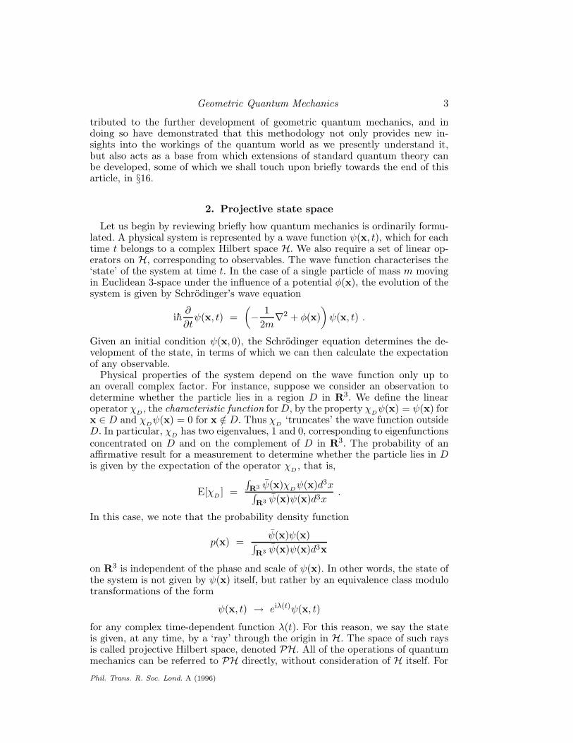
The join of two distinct points ξα and ηα in PH is a complex projective line,represented by points in PH of the form

ψα = Aξα +Bηα ,

where A and B are complex numbers, not both zero. A neat way of characterisingthis line is the tensor Lαβ = ξ[αηβ]. Physically, Lαβ represents the system of allpossible quantum mechanical superpositions of the states ξα and ηα. To see thatLαβ represents a line, consider a finite dimensional case where PH = CPn. Then,because of the skew-symmetry of Lαβ it has 1

2n(n+1) complex components, whichcan be viewed as the line coordinates of the given line. The fundamental propertyof these line coordinates is that their ratios are independent of the choice of thetwo points ξα and ηα, in such a way that all points on the given line are treatedon an equal footing.

The simplest situation in which a probabilistic idea arises in quantum theoryis also the simplest situation in which the concept of the ‘distance’ between twostates arises. The transition probability for the states ξα and ηα determines anangle θ as follows:

cos2 1

2θ =

ξαηαηβ ξβ

ξγ ξγηδ ηδ

.

Clearly, θ is independent of the scale and phase of ξα and ηα. This angle definesa distance between the states ξα and ηα in PH. If the states coincide, then θ = 0;for orthogonal states we have θ = π, the maximum distance.

Suppose we set θ = ds and ξα = ψα, ηα = ψα+dψα. By use of the expression forthe transition probability, expanded to second order, we find that the infinitesimal



ξ η

ξηαα

αα

ηξ

αβL

ξ α

ηα

S

ξ

α

αη

θ

2

CP

PH

1^

^

^

^

Figure 2. Transition probability. The join of two states ξα and ηα in projective Hilbert space PHis a complex projective line CP 1: Lαβ = ξ[αηβ]. The points on Lαβ represent superpositions ofξα and ηα. Such a line is intrinsically a real 2-manifold with spherical topology. The conjugate

hyperplanes ξα and ηα intersect Lαβ at points ξα and ηα in PH. The angle θ determined bythe cross ratio cos2(θ/2) = ξαηαη

β ξβ/ξγ ξγη

δ ηδ induces a metrical geometry on S2, for which θ

is the usual angular distance, and ξα is antipodal to ξα.

distance ds between two neighbouring states is

ds2 = 8ψ[αdψβ]ψ[αdψβ]

(ψγψγ)2,

an expression known to geometers as the Fubini-Study metric (Kobayashi &Nomizu 1969; Arnold 1989). This expression is well-defined both in finite andinfinite dimensions. The introduction of the Fubini-Study geometry illustrateshow the notions of probability and distance become interlinked, once quantumtheory is formulated in a geometric manner. The geodesic distance with respectto the Fubini-Study metric determines the transition probability between twostates. Indeed, the nontrivial metrical geometry of the Fubini-Study manifold isresponsible for the ‘peculiarities’ of the quantum world, and in what follows weshall see various examples of this phenomenon.

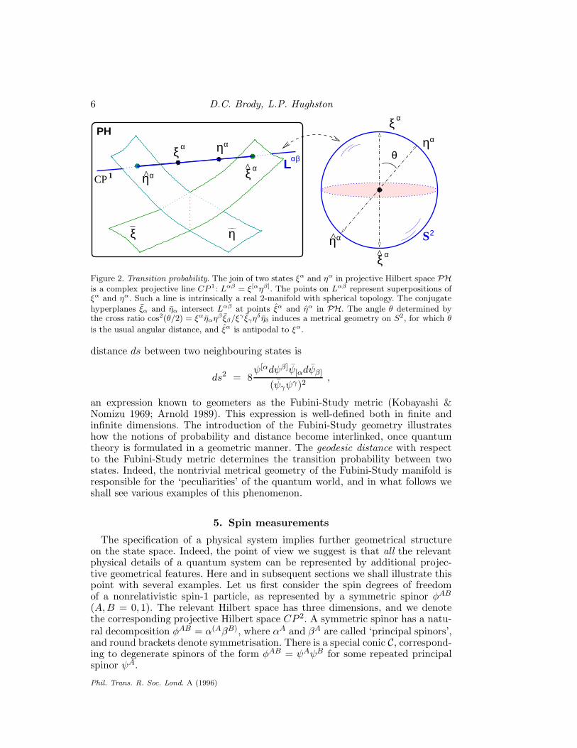
5. Spin measurements

The specification of a physical system implies further geometrical structureon the state space. Indeed, the point of view we suggest is that all the relevantphysical details of a quantum system can be represented by additional projec-tive geometrical features. Here and in subsequent sections we shall illustrate thispoint with several examples. Let us first consider the spin degrees of freedomof a nonrelativistic spin-1 particle, as represented by a symmetric spinor φAB

(A,B = 0, 1). The relevant Hilbert space has three dimensions, and we denotethe corresponding projective Hilbert space CP 2. A symmetric spinor has a natu-ral decomposition φAB = α(AβB), where αA and βA are called ‘principal spinors’,and round brackets denote symmetrisation. There is a special conic C, correspond-ing to degenerate spinors of the form φAB = ψAψB for some repeated principalspinor ψA.



βA

Aα

β

αAαB

B

φ

C

= β(Aν B)

AB=α(AµB)

=AB (AβB)

CP 1

CP 2

φ α

ABφAβ

Figure 3. Spin-1 particle. A symmetric spinor φAB has three independent components whichact as homogeneous coordinates for CP 2. The image of the map C : CP 1 → CP 2, definedby ψA ∈ CP 1 → ψAψB ∈ CP 2 determines a curve C in CP 2. The tangent to C at the

point φAB = αAαB in CP 2 consists of spinors of the form φAB = α(AµB) for some µA. Theintersection of the lines tangent to the points αAαB and βAβB is the point α(AβB). Conversely,once a conic C is specified, a map C−1 is established from CP 2 to point-pairs in CP 1, calledprincipal spinors. The points on C map to degenerate point-pairs. An analogous result holds forspin 2, which has striking applications in gravitational theory, first systematically explored byPenrose (1960).

The identification of C is sufficient to induce the structure of a spin-1 system onthe state space, since through any generic point in CP 2 there are two lines tangentto C, and the corresponding tangent points determine the principal spinors, upto scale, as shown in Figure 3. Alternatively, we can think of a conic C in CP 2

being represented by a map (see, e.g., Semple & Kneebone 1952) from CP 1 toCP 2 such that if (t, u) are homogeneous coordinates on CP 1, we have

C : (t, u) → (t2, tu, u2) ,

where (t2, tu, u2) now represents homogeneous coordinates on CP 2. Because acomplex projective line, in real dimensions, represents a sphere S2 (cf. Figure 2),the specification of the spin direction determines a point on S2, and hence on C.

The conic is required to be compatible with the complex conjugation operationon the state space in the sense that if we conjugate a point of C, then the resultingline is tangent to C. The complex conjugate φAB = α(AβB) of a general state

corresponds to a complex projective line consisting of states of the form PαAαB +QβAβB , where we define αA = ǫABαB and βA = ǫAB βB , with ǫAB the naturalsymplectic structure. The rules for the complex conjugation map c on spinors areas follows:

c(αA) = αA

c(αA) = −αA.

The latter identity arises since c(αA) = c(ǫABαB) = ǫABαB = −αA. Recall that

for any spinor φA we have the relation φA = ǫABφB and φAǫAB = φB, and thatǫAB satisfies ǫAB = −ǫBA and ǫAB = ǫBA. If we take the complex conjugate of astate on C, the resulting line is tangent to the conic at a point, which we call theconjugate of the original point on C. This establishes a Hermitian correspondence



Spin 1

CP2

θθ

ZS 0=

AB

(A ψB)

ψAψB

AB=λAλBψBAψ-1

1

0θ

-1=S Z

S Z=1

X

ψ

φ

φ

C

Figure 4. Spin measurement. The state space of a spin 1 system has a conjugation relation thatassociates to each point ψAψB on the special conic a conjugate point ψAψB . The antipodalpoints ψA and ψA on the corresponding 2-sphere select a direction in Euclidean 3-space. Thethree points ψAψB, ψAψB, and ψ(AψB) are eigenstates of the spin operator Sz associated withthis axis. The corresponding geodesic distances θ1, θ−1, θ0 to a generic state X ∈ CP 2 determinethe probabilities of the measurement outcomes for Sz for a particle in the state X.

between pairs of points on C. For a state φAB = ψAψB the conjugate line consistsof states of the form λ(AψB) for arbitrary λA. This line touches the conic C atthe point ψAψB .

Each choice of a point on C, as noted above, determines a spin axis. For anyspin axis there are three possible spin states, with eigenvalues 1,−1 and 0. Thespin eigenstates are the points ψAψB and ψAψB on C, having the eigenvalues 1and −1, together with a third point ψ(AψB) obtained by intersecting the linestangent to the conic C at the other two points, corresponding to eigenvalue 0, asindicated in Figure 4.

When a spin measurement is made, the initial state corresponds to a genericpoint X in CP 2, and the measurement is defined by a spin axis. The state then‘jumps’ from its initial point to one of the three spin eigenstates associated withthe choice of axis. Quantum theory, as such, states nothing about the “mecha-nism” whereby this jump is achieved. We can, however, compute the probabil-ities, and describe the result in geometrical terms. First we calculate the dis-tance from X to each of the three spin eigenstates, by use of the Fubini-Studymetric. This gives us three angles θ1, θ−1, and θ0. For each angle we computeP (θ) = 1

2 (1+cos θ), which gives us the probability of transition to that particularstate. It is not obvious that the three probabilities computed in this way sum upto one, given any initial state in which the measurement is performed, but theydo: this is a ‘miracle’ of the Fubini-Study geometry.

6. Spin-32 and the twisted cubic

We have seen that in the case of a projective plane, there is a conic C, corre-sponding to degenerate spinors obtained by a special map from a projective lineto a plane. On the other hand, in three-dimensional projective space CP 3 thereare two different kinds of locus to be considered, each of which is in some respectsa proper analogue of the conic, namely, the quadric surface Q and the twistedcubic curve T . While a surface is the locus of a variable point of space which hastwo complex degree of freedom, a curve is the locus of a variable point of space



of one complex degree of freedom. When viewed as the state space of a quantummechanical system, the quadric surface in CP 3 characterises the disentangledstates of a pair of spin-1

2 particles, the geometry of which we shall study in somedetail in subsequent sections.

The twisted cubic, the simplest nonplanar curve in projective geometry, on theother hand, plays an essential role in the geometry of the state space of a spin-3

2particle. Analogous to the conic curve, the twisted cubic can be represented by amap from CP 1 to CP 3 of the form

T : (t, u) → (t3, t2u, tu2, u3) ,

where (t3, t2u, tu2, u3) represents homogeneous coordinates of points on T in CP 3.If follows that T is an algebraic space of the third order, which meets a genericplane of CP 3 in three points.

In order to proceed further, we introduce a spinorial notation and let the sym-metric spinor ψABC = ψ(ABC) denote homogeneous coordinates on CP 3. Then,the twisted cubic arising naturally here is determined by the relation

τAB := ψCD(AψCDB) = 0 ,

where the indices on ψABC are raised and lowered according to the standardconventions, so for example, ψCD

B = ǫABψACD, and so on. The general solution

to the algebraic relations given by τAB = 0 takes the form ψABC = ξAξBξC forarbitrary ξA (Hughston, Hurd & Eastwood 1979).

The specification of a twisted cubic T in CP 3 induces a null polarity on the

SZ=3/2

SZ=1/2

=-3/2ZS

=-1/2ZS

ψ ψ

ψA

C)B(A

ψC)Bψ(A

ψA

ψψψ

ψ

ψB

T

ψ C

B C

Figure 5. The twisted cubic curve as a system of spin states. The quantum phase space for aspin 3/2 particle contains a preferred twisted cubic T which is self-conjugate in the sense thatthe complex conjugate plane corresponding to any point on T necessarily osculates the curve atsome other point on T . The points of T are those states which have an eigenstate of spin 3/2relative to some choice of spin axis. Each point of T corresponds to a choice of spin axis anddirection.



state space, i.e., a natural correspondence between points and planes such thatthe polar plane of a given point actually includes that point. The null polarity isgiven by the map

ψABC → ψABC = ǫAP ǫBQǫCRψPQR ,

and it follows as an elementary spinor identity that ψABCψABC = 0 for any choiceof ψABC . In the case of a point ψABC = ξAξBξC on T , the corresponding polarplane intersects T solely at that point, with a three-fold degeneracy, and is calledthe osculating plane at that point.

Each choice of ξA, i.e., a point on T , determines a spin axis. For each spin axis,there are four possible spin eigenstates with eigenvalues 3

2 , 12 , −1

2 , and −32 . Two of

the spin states, corresponding to eigenvalues ±32 , lie on T itself. These two states

can be written ψAψBψC and ψAψBψC , where ψA = ǫABψB and ψB = c(ψB).The choice of ψA determines the spin axis. The complex conjugate of the state

ψABC = ψAψBψC on the twisted cubic T is the plane ψABC = ψAψBψC in CP 3,and this plane is tangent to T at the point ψAψBψC . On the other hand, throughthe point ψAψBψC there is a unique line tangent to T , and this line intersects theplane ψAψBψC at a point, given by ψ(AψBψC). This point is the spin 1

2 eigenstatewith respect to that choice of axis. Conversely, the tangent line to T at the spin−3

2 state ψAψBψC intersects the tangent plane of T at ψAψBψC at the point

ψ(AψBψC), which is the spin −12 state.

An interesting feature of the twisted cubic geometry arises from the fact thatfor any symmetric spinor ψABC we have the relation

τABψABC = 0 ,

which follows from the spinor identity ǫ[ABǫC]D = 0. This relation implies that

through any point ψABC in CP 3 − T , i.e., a point off the curve, there exists aunique chord of T . This follows from the fact that, providing τAB is nondegener-ate, the condition τABψ

ABC = 0 implies a relation of the form

ψABC = uξAξBξC + vηAηBηC

for some ξA and ηA corresponding to a pair of spin axes such that ξAηA 6= 0,

where (u, v) are homogeneous coordinates on CP 1. It follows that an arbitraryquantum state ψABC in CP 3 −T admits a unique characterisation in terms of asuperposition of a pair of spin-3

2 eigenstates corresponding to distinct spin axes.If τAB is degenerate, then the chord reduces to a tangent line to T with a doublepoint at the intersection, and ψABC has a unique representation of the formψABC = ξ(AξBηC).

A similar analysis can be pursued in connection with the geometry of a spin-2system, for which the state space is CP 4, endowed with a self-conjugate rationalquartic curve. The geometry of this curve is closely related to the Petrov-Piraniclassification of gravitational fields.

7. Geometry of entanglement

Now consider a more elaborate set-up: the spin degrees of freedom of an entan-gled pair of spin-1

2 particles. The generic two-particle state ψAB for a pair of such



CP 3 1CP

SZ=0 ψBAψ

(Aψ B)

CP2Z

Z

ψ[A ψB]

ψ

CP1

ψAψB

ψBAψψAψB

S=1C

S=0

Q e p

Figure 6. Quantum entanglement. The quantum phase space of an electron-positron system con-tains a point Z for total spin 0, and a projective hyperplane Z for total spin 1. The disentangledstates have indefinite total spin, and comprise a quadric Q ruled by two systems (electron andpositron) of linear generators. Once a spin axis is chosen, the join of Z with the state of totalspin 1 and Sz = 0 intersects Q in a pair of points, corresponding to the possible measurementoutcomes of the spin of the electron relative to the axis.

particles (e.g., an electron and a positron) has a 4-dimensional Hilbert space, andthe state space is CP 3. There is a preferred point Z in CP 3, corresponding tothe singlet state of total spin 0, for which ψAB = ψ[AB]. The conjugate plane Zcontains the triplet states of total spin 1, for which ψAB = ψ(AB). We note thatZ is endowed with a conic C, each point of which defines a spin axis. There isalso a special surface Q ∈ CP 3, given by the quadratic equation

ǫACǫBDψABψCD = 0 ,

consisting of states of the disentangled form ψAB = ξAηB , representing an em-bedding of the product of the state spaces of the individual spin-1

2 particles. Thestates off the quadric are the entangled states.

Suppose we start with a combined state of total spin 0 for the two particles,and we measure the spin of the first particle (say, the electron) relative to a givenchoice of axis. This will disentangle the state, so the result lies on Q. The choiceof axis and orientation determines a point and its conjugate on the conic C. Thetangents to the conic at these points intersect to form a third point off the quadricbut in the plane of total spin 1, corresponding to a triplet state of eigenvalue 0relative to the axis. We join that state to the starting state Z, and the resultingline intersects Q at a pair of points, as shown in Figure 6.

The two disentangled states thus obtained represent the possible measurementoutcomes. The quadric Q has two systems of generators, corresponding to theelectron and positron state spaces. Through each point of Q there is a unique‘electron generator’ and a unique ‘positron generator’. An electron generator rep-resents a fixed electron state, each point on it corresponding to a possible positronstate. The two points constituting the possible outcomes of the spin measurement



of the electron have the property that their electron generators hit respectivelythe two chosen points on the conic that define the spin axis. The measurementresult for which the electron generator hits the spin up state on the conic is the‘electron spin up and positron spin down’ outcome, whereas the other one is the‘electron spin down and positron spin up’ outcome.

In a more general situation, the idea of quantum entanglement is characterisedgeometrically by the fact that complex projective space admits a Segre embeddingof the form

CPm × CPn → CP (m+1)(n+1)−1 .

Here we regard both CPm and CPn as representing the state space of two sub-systems, respectively, while CP (m+1)(n+1)−1 represents the state space of thecombined system. One can argue that this is the main feature of quantum me-chanics that has no analogue is classical physics. That is to say, classically, thestate space of a combined system is given by the product of the state spaces ofthe subsystems, which has a moderate dimensionality when compared with thesituation of the quantum state space for a combined system.

8. Measure of entanglement

The set up indicated above suggests a methodology according to which a mea-sure δ(ψ) can be assigned to the degree of entanglement exhibited by a given purestate ψ. This is a topic currently of great interest in quantum physics (cf. Linden,et. al. 1999). Let us consider the general case of a finite dimensional two-particlestate space CPn containing a subvariety V m ⊂ CPn, where V m = CP j × CP k

and n = (j + 1)(k + 1) − 1. The variety V m represents the disentangled statesof the two particles, and is given by the product of the respective single particlestate space CP j and CP k.

We propose, as a measure of entanglement for a generic pure state ψ ∈ CPn,the use of the geodesic distance from the given state ψ to the nearest disentangledstate. The distance δ is measured with respect to the Fubini-Study metric.

Clearly, δ is a natural measure in the sense that it depends only on the Segreembedding of the variety V m and no additional structure apart from the givenmetrical geometry of CPn. Furthermore, we can demonstrate that δ is invariantunder any unitary transformation of CPn that is also an automorphism of V m,i.e., transformations that preserve the disentangled state space. It should be evi-dent that essentially the same construction applies to the case of entangled statesof any number of particles. We do not require that the particles are necessarilyof the same type.

As a specific illustration, we consider the system described in §7 consisting oftwo spin-1

2 particles, where the state space is CP 3 and the space V 2 of disentan-

gled states is a quadric Q ⊂ CP 3. Suppose we write ψAB for a generic state, andψAB for the corresponding complex conjugate hyperplane. Then the distance δfrom ψ to Q is determined by the relation κ = 1

2(1 + cos δ), where κ is the crossratio

κ =(ψABXAB)(XCDψCD)

(ψABψAB)(XCDXCD),

and XAB ∈ Q maximises κ for the given state ψAB . The cross ratio κ is the Dirac



transition probability from the state ψAB to the state XAB , and our goal is tofind the states on Q for which the transition probability from ψAB is maximal.

We shall turn to the details of the maximisation problem in a moment, in §10,since these are of interest, but here first we present the solution. Let us writeψCD := ǫACǫBDψ

AB and ψAB := ǫACǫBDψAB , where the antisymmetric spinorǫAB satisfies the usual relation ǫABǫ

AC = δCB . Then the solution for κ is given by

κ = 12(1 + γ), with

γ =

√

1 − (ψABψAB)(ψCDψCD)

(ψABψAB)2.

We note that γ is independent of the scale of ǫAB and lies in the range 0 ≤ γ ≤ 1.The inequality satisfied by γ follows from a general result that for any element zin a complex vector space with a Hermitian inner product we have the Hermitianinequality (z · z)2 ≥ (z · z)(z · z). This can be seen by writing z = a + ib, wherea and b are real, and then checking that the purported relation reduces to theSchwartz inequality (a · b)2 ≤ (a · a)(b · b).

If the point ψAB lies on the quadric Q, we have ψABψAB = 0, and hence

γ = 1, which implies κ = 1, from which it follows that the distance to the quadricis δ = 0. On the other hand, for a maximally entangled state the inequality issaturated at γ = 0, and thus gives κ = 1/2, which implies δ = π/2.

The interpretation of this result is as follows. We recall that for orthogonalstates the Fubini-Study distance is π, the greatest distance possible for two states.On the other hand, the maximum distance an entangled state can have from theclosest disentangled state, in the case of two spin-1

2 particles, is π/2. For example,

with respect to a given choice of spin axis, the spin 0 singlet state ǫAB can beexpressed as an antisymmetric superposition of two disentangled states, i.e., anup-down state and a down-up state. The two disentangled states are mutuallyorthogonal, and the singlet state lies ‘half way’ between them.

9. Hermitian polar conjugation

Now, let us consider the geometry of this situation in more detail. There isa well-known construction in algebraic geometry according to which a properquadric locus in CP 3 induces a polarity on this space — a one-to-one correspon-dence between points and planes. Reverting briefly to the notation of §3, let uswrite ψα for the homogeneous coordinates of a point in CP 3, and Qαβψ

αψβ = 0for the quadric. We assume that the quadric is nondegenerate, i.e., proper, in thesense that det(Qαβ) 6= 0. Then for any state ξα ∈ CP 3 it follows that ξα := Qαβξ

β

is nonvanishing. The locus ξαψα = 0 defines the polar plane of the point ξα with

respect to the quadric Qαβ. Since Qαβ is nondegenerate, there is a unique inverse

Qαβ satisfying QαγQγβ = δβ

α, and thus for any plane ηα in CP 3 we can define a

polar point ηα := Qαβηβ. The operation is involutory in the sense that the polarpoint of the polar plane of a given point is that point.

One way of constructing the polar plane of a point ξ is as follows. Let L be anarbitrary line Lαβ = ξ[αζβ] through ξ. Then L intersects Q twice, say, at pointsA and B. Now suppose we consider the harmonic conjugate ξ∗ of ξ, on the lineL, with respect to the points A and B. This is the unique point ξ∗ on L such



ψ

Q

ψ

ψCP

CP 2

3

X

C

α

αα

α

X α

Figure 7. Hermitian polar conjugation and the construction of extremal disentangled states. Givenany entangled state ψα we can form another state ψα given by the harmonic conjugate of thecomplex conjugate plane of ψα with respect to the quadric Q. The points on Q nearest to andfurthest from ψα are given by the intersection points Xα and Xα of Q with the line joining ψα

and ψα.

that we have

ξ, ξ∗;A,B = −1

for the cross ratio. Then, as we vary L, the locus of ξ∗ sweeps out a plane, andthis is the polar plane ξ. The polar plane ξ intersects Q in a conic C with theproperty that any line drawn from ξ to C touches Q tangentially.

Conversely, if we consider all the lines through ξ that touch Q tangentially,then the union of the intersection points is the conic C, which lies in a uniqueplane, the polar plane ξ. A point lies on its polar plane iff the point itself lies onthe quadric, in which case the polar plane of the point is the tangent plane atthat point. In that case, the conic C degenerates into a pair of lines, given by thetwo generators of the quadric through the given point.

In the quantum mechanical situation we require further that the quadric Qαβ

be Hermitian in the sense that Qαβ = Qαβ and Qαβ = Qαβ. This ensures that thecomplex conjugate ket-vector |¯x〉 of the polar bra-vector 〈x| of a given ket-vector|x〉 agrees with the polar ket-vector |˜x〉 of the complex conjugate bra-vector 〈x| ofthe given ket-vector |x〉. It follows that complex conjugate ket-vector of the polarbra-vector of a disentangled state is also disentangled, and that the polar ket-vector of the complex conjugate bra-vector of a disentangled state is disentangled.

The situation described so far applies to the consideration of any pair of two-state systems, whether or not these systems are of the same type. For example, wemight consider a simple toy model in which a lepton is regarded as a compositeconsisting of a neutral spin-1

2 particle and a spin-0 flavour doublet that deter-mines whether the lepton is an electron or a muon. Then one might explore the



properties of the entangled state given by a superposition of a spin-up electronwith a spin-down muon, the spin state being given with respect to some choiceof axis. What distinguishes the state space of a pair of spin-1

2 particles is the ex-istence of a preferred singlet state Zα. This state is required to be self-conjugatepolar with respect to the quadric in the sense that Zα = QαβZ

β.

10. Maximal entanglement

We are now in a position to present a more geometrical construction for thesupremum of the cross-ratio κ under the given constraint. Given the entangledstate ψα we wish to find the state Xα ∈ Q that maximises the cross ratio

κ =(ψαXα)(Xβψβ)

(ψαψα)(XβXβ).

In fact, suppose we define ψα := Qαβψβ , the polar state of the complex conjugatehyperplane ψα. Then we can show that the states on Q that are maximally andminimally distant to the given state ψα are collinear with ψα, and are complexconjugate polar to one another in the sense that ψα has to be of the form

ψα = pXα + qQαβXβ

where Xα is the point on Q closest to ψα, so |p| ≥ |q|. This can be verified,for example, by maximising κ with respect to Xα subject to the constraintQαβX

αXβ = 0, using a Lagrange multiplier technique. Then if we define λ = p/qit follows by a direct substitution that

κ =λλ

1 + λλ.

Since λλ ≥ 1, it follows, further, that 12 ≤ κ ≤ 1. On the other hand, we can also

verify by direct substitution that the invariant ρ defined by

ρ =(Qαβψ

αψβ)(Qγδψγψδ)

(ψγψγ)2,

which is independent of the scale of Qαβ, depends on p and q only through λ,and is given by the formula

ρ =4λλ

(1 + λλ)2.

Then it is not difficult to see that κ is indeed of the desired form κ = 12 (1 + γ)

with

γ =√

1 − ρ.

That establishes the the validity of the expression indicated earlier for the mini-mum distance

δ = cos−1√

1 − ρ

from the given state ψα to the quadric of disentanglement.The maximally entangled states are those for which |λ| = 1, for which apart



C

ψ ψB

ψAψB

A

0S=

SZ= 0

C’

CP 3

’C

Q

Figure 8. Maximally entangled states. Through any conjugate pair of disentangled states on Qthere exists a complex projective line containing the S = 0 singlet and an Sz = 0 triplet statefor some choice of z-axis. The singlet and triplet states lie on an equatorial circle at a distance ofπ/2 from the disentangled states which are orthogonal to one another and thus lie on oppositepoles. All the points on this equatorial circle are maximally entangled. The trajectory of theentangled triplet states corresponding to different spatial directions is a conic C′, which has atopology of a sphere. Hence the space of maximally entangled states has the structure of S2×S1.

from an overall irrelevant scale factor ψα is thus necessarily of the form

ψα = eiθXα + e−iθQαβXβ .

Such states are self-conjugate in the sense that ψα = Qαβψβ. Conversely, given

any disentangled state Xα we see that there exists a one-parameter family ofmaximally entangled states at a distance π/2 from it. This one-parameter familyis given by the equatorial circle of the complex projective line obtained by joiningXα to the conjugate entangled state QαβXβ , to which Xα is orthogonal.

Thus, for example, if XAB = ξAηB is a disentangled state of two spin-12 par-

ticles, then we obtain the one-parameter family of maximally entangled statesgiven by ψAB = eiθξAηB + e−iθ ξAηB where ξA := ǫAB ξB and ηB := ǫBAηA. Forany value of θ these states are at a distance of π/2 from XAB .

A special case of interest arises when ηB = ξB and ηA = −ξA. In that case,reverting to the notation of the previous section, we have ψAB = eiθψAψB −e−iθψAψB . Then for θ = 0 we obtain the spin 0 singlet state for which ψAB ∝ ǫAB;whereas for θ = π we get the Sz = 0 spin 1 triplet state for which ψAB ∝ ψ(AψB).

More generally, if ψα is an arbitrary maximally entangled state, then considerthe conic K that arises when we intersect the plane ψα with the quadric Q. Thisconic is conjugate self-polar in the sense that for any point πα on K the complexconjugate plane πα is tangent to the quadric at a point πα on K. Now, supposewe consider the locus L of points generated by the intersection of the tangentlines to πα and πα in the plane ψα as we vary πα. For any point P in L the joinof that point with ψα intersects Q in a pair of points Xα and Xα, both of which



are at a distance δ = π/2. By varying P we obtain all points on Q at a distanceπ/2 from ψα.

Finally, let us consider the case of sub-maximally entangled states. In thissituation the relation between ψα and Xα is invertible, since providing |λ| > 1there exist complex numbers r and s such that

Xα = rψα + sQαβψβ.

We can solve this for the ratio µ = r/s by imposing the condition QαβXαXβ = 0,

leading to the quadratic equation µ2Qαβψαψβ + 2µψαψα + Qαβψαψβ = 0, for

which the roots are given by

µ =−1 ±√

1 − qq

q,

where q := Qαβψαψβ/ψγ ψγ . The positive root gives the point on Q nearest to

ψ, and the negative root gives the most distant disentangled state. We note thatthe terms here are so constructed that the solution for Xα is independent of theoverall scale and phase of ψα, as expected.

11. Schrodinger evolution

As the examples above indicate, the geometry of quantum mechanics is veryrich, once specific physical systems are brought into play, even when there are onlya few degrees of freedom. This picture can be further developed by considerationof the dynamics of a quantum system, which can be pictured as a vector field onthe state manifold. Such a vector field generates a symmetry of the Fubini-Studygeometry, i.e., an action of the projective unitary group.

In the case of an (n + 1)-dimensional Hilbert space, the state space is CPn,which can be viewed as a real manifold Γ of dimension 2n, with a symmetry groupof dimension n(n+ 2), generated by a family of n(n+ 2) Killing vector fields. Ageneric Killing field on Γ has n+ 1 fixed points, corresponding to eigenstates ofthe given Hamiltonian.

In the case of a 2-dimensional Hilbert space, the state space is CP 1, and thespecification of a Killing field selects out a pair of polar points on S2, correspond-ing to energy eigenstates E1 and E2. The relevant symmetry is then given by arigid rotational flow about this axis, the angular frequency being determined byPlanck’s formula E2 − E1 = hω. In the case of the state space CPn, the n + 1fixed points of a given Killing field are linked by a figure consisting of 1

2n(n+ 1)spheres, for which the fixed points act as polar points, in pairs. These spheresrotate respectively with angular frequencies

Ei − Ej = hωij ,

where Ei (i = 1, 2, · · · , n+ 1) labels the energy of ith eigenstate. The dynamicaltrajectories in Γ are determined by the specification of the fixed points, along withthe associated angular frequencies. Even in the case of a simple spin 1 system,the geometry of the state space is intricate, given by a 4-dimensional manifoldcontaining three 2-spheres touching one another at the poles, and spinning atthree distinct frequencies.

If the frequencies are not commensurate in the sense of being rational multiples



Energy surface

T

Sn-1

Γ 2n

*

n

Figure 9. Foliation of the state space and quantum dynamical trajectories. The quantum statespace is foliated by level surfaces of the expectation of the Hamiltonian operator. Each point onsuch a surface is parameterised by a family of n phase variables, n− 1 angular coordinates, andone energy variable. The Schrodinger evolution preserves the energy and the angular coordinatesof a given initial state (point), and the resulting dynamical trajectory is thus confined to then-torus Tn. If the ratios Ei/Ej of the energy eigenvalues are irrational, then the trajectory onTn does not close.

of each other, then the Killing orbits do not close except on the three specialspheres, and the generic dynamical trajectory, starting from some initial pointin the state space, is doomed to evolve to eternity without ever returning to itsorigin. More specifically, we can view the quantum state space CPn as a realmanifold Γ

2n of dimension 2n. Then, we can consider a foliation of Γ2n by level

surfaces of constant energies. The specification of the energy thus determines oneof the 2n real coordinates on the state space. The remaining 2n − 1 coordinatescan be identified (Brody & Hughston 1999b) with n−1 angular coordinates and nphase variables. In other words, each energy surface has the structure of a productspace of an n-torus and an (n− 1)-sphere, i.e., T n ×Sn−1. Given an initial pointon one of the energy surfaces, the dynamics induced by the Schrodinger evolutionwill confine that point to the torus that contains the initial state. In other words,the angular variables of the initial state remain unchanged under the action of theprojective unitary group induced by the given quantum Hamiltonian. It follows,therefore, that the Schrodinger evolution is at best merely quasiergodic on theenergy surface.

12. Quantum Hamiltonian dynamics

This line of argument can be taken further by studying the quantum trajec-tories on Γ by use of differential geometry. When viewed as a real manifold, thestate space is endowed with a Riemannian structure, given by a positive definitesymmetric metric gab, a symplectic structure, given by an antisymmetric tensorΩab, and a complex structure, given by a tensor Ja

b, satisfying

JacJ

cb = −δa

b .



These structures are required to be compatible in the sense that Ωab = gacJcb

and ∇aJbc = 0, where ∇a is the covariant derivative associated with gab. Here

we use Roman indices (a, b, · · ·) for tensorial operations in the tangent space ofΓ. The compatibility of gab, Ωab, and Ja

b makes Γ a Kahler manifold. For somepurposes it suffices to assume that the metric gab and the symplectic structureΩab are only weakly nondegenerate in the sense that for any vector fields ξa, ηa

on Γ, ξagab = 0 implies ξa = 0 and ηaΩab = 0 implies ηa = 0. The fact that ininfinite dimensions the Fubini-Study metric and symplectic structure are stronglynondegenerate (Marsden & Ratiu 1999) means that many of the geometrical con-structions carried out in finite dimensions carry through to the general quantumphase space.

The additional ingredient required for the specification of the dynamics is aHamiltonian function H(x) on Γ. Then the general dynamical trajectories on Γ

are given by1

2hΩabdx

b = ∇aHdt .

The Schrodinger trajectories on Γ are given by a subclass of the general Hamil-tonian trajectories, namely, those for which the Hamiltonian function H(x) is ofthe special form

H(x) =ψα(x)Hα

βψβ(x)

ψγ(x)ψγ(x).

Here, ψα(x) denote homogeneous coordinates for the corresponding point x inthe projective Hilbert space. Thus for a Schrodinger trajectory, H(x) is the ex-pectation of the Hamiltonian operator in the pure state to which the point xcorresponds. In contrast with classical mechanics, where the phase space oftenhas an interpretation in terms of position and momentum variables, in quantummechanics the points in phase space correspond to pure quantum states.

Quantum observables are intimately related to the metrical geometry of Γ.The distinguishing feature of a quantum Hamiltonian function H(x) is that theassociated symplectic gradient flow ξa = dxa/dt is a Killing field, i.e., ∇(aξb) = 0.Indeed all Killing fields on Γ arise in this way through quantum observables. TheKilling fields generate the symmetries of the Fubini-Study metric gab.

In the case of finite dimensions, we can say more about the quantum observ-ables that generate isometries on the Fubini-Study manifold. If H(x) is a linearobservable function, then in finite dimensions it is necessarily defined globally onΓ. In fact, one can show that such functions correspond to global solutions of thecharacteristic equation

∇2H = (n+ 1)(H −H) ,

where ∇2 is the Laplace-Beltrami operator on Γ, H = Hαα/(n+1) is the uniform

average of the eigenvalues of Hαβ , and 2n is the real dimension of Γ. Conversely,

if we are given a Killing field ξa, the corresponding observable function H(x) canbe recovered, up to an additive constant, via the relation

hΩab∇aξb = 2(n+ 1)(H − H) ,

which follows directly from the characteristic equation if we make use of thefact that hξa = 2Jb

a∇bH. We note, incidentally, that in the Kibble-Weinberg



theory, a general nonlinear quantum observable is a function on Γ such thatthe characteristic equation is not satisfied. As a consequence, the correspondingsymplectic gradient flow is no longer a Killing field.

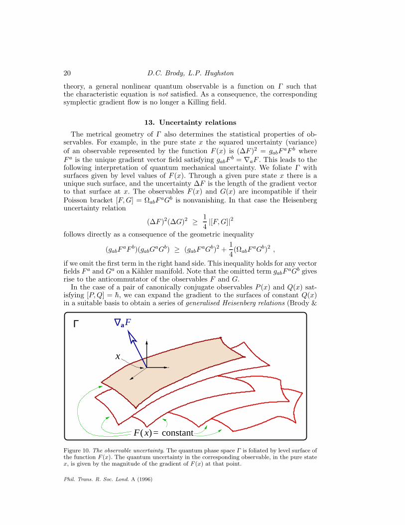
13. Uncertainty relations

The metrical geometry of Γ also determines the statistical properties of ob-servables. For example, in the pure state x the squared uncertainty (variance)of an observable represented by the function F (x) is (∆F )2 = gabF

aF b whereF a is the unique gradient vector field satisfying gabF

b = ∇aF . This leads to thefollowing interpretation of quantum mechanical uncertainty. We foliate Γ withsurfaces given by level values of F (x). Through a given pure state x there is aunique such surface, and the uncertainty ∆F is the length of the gradient vectorto that surface at x. The observables F (x) and G(x) are incompatible if theirPoisson bracket [F,G] = ΩabF

aGb is nonvanishing. In that case the Heisenberguncertainty relation

(∆F )2(∆G)2 ≥ 1

4|[F,G]|2

follows directly as a consequence of the geometric inequality

(gabFaF b)(gabG

aGb) ≥ (gabFaGb)2 +

1

4(ΩabF

aGb)2 ,

if we omit the first term in the right hand side. This inequality holds for any vectorfields F a and Ga on a Kahler manifold. Note that the omitted term gabF

aGb givesrise to the anticommutator of the observables F and G.

In the case of a pair of canonically conjugate observables P (x) and Q(x) sat-isfying [P,Q] = h, we can expand the gradient to the surfaces of constant Q(x)in a suitable basis to obtain a series of generalised Heisenberg relations (Brody &

∆

aΓ F

constant=)x(F

x

Figure 10. The observable uncertainty. The quantum phase space Γ is foliated by level surface ofthe function F (x). The quantum uncertainty in the corresponding observable, in the pure statex, is given by the magnitude of the gradient of F (x) at that point.



Hughston 1996, 1997, 1998a,b), an example of which is

(∆P )2(∆Q)2 ≥ 1

4h2

(

1 +(µ4(P ) − 3µ2(P )2)2

µ6(P )µ2(P ) − µ4(P )2

)

,

where µk(P ) = 〈(P − 〈P 〉)k〉 is the kth central moment of the observable P inthe state x. This inequality has the following statistical interpretation. Supposethat we are given an unknown quantum state of a particle, parameterised by itsposition q, and that we wish to estimate the position of the particle by a suitablemeasurement. The observable function corresponding to the parameter q is thengiven by Q, and the statistical estimation of q via measurement on Q gives rise toan inevitable variance lower bound, expressed in terms of a certain combinationof the moments µk(P ) of the momentum distribution associated with the givenstate. Likewise, if we consider momentum estimation, then the correspondingvariance lower bound is given by the moments of the position Q.

14. Geometric phases

An interesting interplay between the quantum dynamical trajectories and theuncertainty relations was pointed out by Aharonov & Anandan (1990). In par-ticular, it follows from the projective Schrodinger equation hΩabdx

b = 2∇aHdtand the expression for the line element ds2 = gabdx

adxb that the ‘speed’ in thestate space Γ along the dynamical trajectory at the point x is given by

hds

dt= 2∆H ,

where ∆H is the energy uncertainty in the given state. For example, in the caseof a 2-state system with eigenstates at the poles of a 2-sphere, the quantumevolution corresponds to a rigid rotation of the sphere, with constant angular

θ dtds =

2

1E

E

h (E2-E1) sinθ

Figure 11. The Anandan-Aharonov relation. The quantum evolution of a 2-state system corre-sponds to the rigid rotation of a 2-sphere with angular frequency hω = E2 − E1. The speed ofthe trajectory is greatest at the equator, which consists of states of maximal energy uncertainty.



frequency, for which the speed is greatest at the equator, corresponding to statesof maximum uncertainty.

This result is related to properties of the geometric phase introduced by Berryand subsequently applied in many situations (Simon 1983; Berry 1984; Uhlmann1986, see also Shapere & Wilczek 1989). Consider a closed path γ in the quan-tum phase space. If γ is a standard dynamical trajectory, then it correspondsto a closed Killing orbit, but we shall allow for the possibility of more generalpaths, e.g., as might be generated by a time-dependent Hamiltonian operator.The geometric phase associated with such a cyclic evolution is given by

β[γ] =

∫

ΣΩabdx

a ∧ dxb ,

where Σ is any real 2-surface in Γ such that γ = ∂Σ. Owing to the relation∇aΩbc = 0, it follows from Stokes’ theorem that the value of β[γ] is independent

ttt

Γ Γ

H~ ~

H

P P

β[γ ]β[γ ]

γγ

P−1[γ ]

21

1

1

2

2

2

P [γ ]−11

Figure 12. The horizontal lift of a quantum trajectory and Poincare’s invariant integral. TheBerry phase β[γ] associated with a general cyclic trajectory γ in the quantum phase space Γ isgiven by the integral of the symplectic form Ωab over a 2-surface Σ spanning γ. This integralmeasures the phase change that develops in the horizontal lift of γ to the corresponding pathP−1[γ] in the Hilbert bundle H over Γ. If the cyclic trajectory subsequently evolves unitarilyin time, then β[γ] is the quantum mechanical integral invariant of Poincare. As a consequence,we have β[γ1] = β[γ2]. This result is valid even if we relax the unitarity condition and considernonlinear dynamics of the Kibble-Weinberg type.



of the choice of surface Σ spanning the loop γ, and can be given the followinginterpretation.

The punctured Hilbert space H = H − 0, obtained by deleting the origin,is a fibre bundle over Γ. Therefore, given a trajectory γ in Γ, we can form acorresponding trajectory P−1[γ] in H, called horizontal lift of γ. This is obtainedby solving the modified Schrodinger equation

ih∂ψα

∂t= (Hα

β − E[H]δαβ )ψβ ,

where E[H] is the expectation of the Hamiltonian in the state ψα. Despite itsnonlinearity, the modified Schrodinger equation is physically natural inasmuch asits stationary states are energy eigenstates. In this connection, it is worth drawingattention to the fact that in the case of the modified Schrodinger dynamics, thetime independent Schrodinger equation

Hαβψ

β = E[H]ψα

follows directly from the stationary state requirement, without the introductionof the so-called correspondence principle E[H] ↔ ih∂t.

The horizontal lift is characterised by the condition that the tangent to thecurve P−1[γ] in H, given by ∂ψα/∂t, is orthogonal to the fibre direction ψα, sowe have ψα∂ψ

α/∂t = 0.In the case of a closed loop γ, β[γ] measures the phase change in ψα over the

corresponding circuit in P−1[γ]. If the given loop γ in Γ subsequently evolvesin time, then β[γ] is a quantum mechanical analogue of the Poincare integralinvariant (cf. Arnold 1989). We note, incidentally, that the notion of geometricphase discussed here also applies to nonlinear quantum mechanics, for which theHamiltonian H(x) does not satisfy the characteristic equation for linear observ-ables.

15. Mixed states

Phase space geometry sheds some interesting light on the role of probability inquantum mechanics. There are at least two situations where probability distri-butions on the state manifold Γ have to be considered. One is in the descriptionof the statistical properties of a measurement outcome; the other is in quantumstatistical mechanics.

In both cases, the state of the system can be characterised by a probabilitydensity function ρ(x) on Γ, in terms of which the expectation of any functionF (x) on Γ can be written

E[F ] =

∫

Γ

ρ(x)F (x)dx.

We think of F (x) as representing the expectation of the corresponding observable,conditional on the pure state x. Then E[F ] is the unconditional expectation, wherewe average F (x) over the pure states, weighting with the density ρ(x). A purestate arises if ρ(x) is a δ-function concentrated on a point in Γ. Consider theexample of a measurement where initially the system is in a pure state X, andthe observable has a finite number of eigenstates, as in the case of a spin-1 system



when we measure the spin along an axis. The result of this measurement is one ofthe three spin eigenstates, and these arise with probabilities determined by theFubini-Study distance. Thus the density function ρ(x) for the state of the systemafter a measurement is given by a sum of three δ-functions, concentrated at theeigenstates, weighted by these probabilities.

In the case of a quantum observable, the unconditional variance of F (x) in ageneral mixed state ρ(x) is given by

V[F ] =

∫

Γ

ρ(x)(F (x) − E[F ])2dx+

∫

Γ

ρ(x)(gabFaF b)2dx .

A further simplification emerges by virtue of the special form of a linear observ-able, for which we have E[F ] = ρα

βFβα , where

ραβ =

∫

Γ

ρ(x)ψβ(x)ψα(x)

ψγ(x)ψγ(x)dx

is the density matrix associated with ρ(x). For ordinary linear quantum mechanicsit suffices to consider the density matrix alone, since all statistical quantitiescalculated with ρ(x) reduce to expressions involving ρα

β . Therefore, for certainpurposes we can regard ρα

β itself as representing the state of the system.One should bear in mind, however, that the density matrix ρα

β , which is the

lowest moment of the projection operator in the state ρ(x), does not in generalcontain all the information of the system when we are dealing with nonlinear ob-servables. This follows from the fact that the information of a generic state ρ(x)is contained in the set of all the moments (cf. Brody & Hughston 1999c). Morespecifically, in the case of a nonlinear observable, we must consider a general stateρ(x), pure or mixed, because the density matrix is not sufficient to take the ex-pectation of such an observable. Some specific examples of nonlinear observableshave been studied by Weinberg (1989a,b). The entanglement measure δ intro-duced in §8 provides another explicit example of a nonlinear observable arisingin a natural context. Exclusive consideration of the density matrix in a nonlinearsetting can lead to paradoxical and apparently nonphysical conclusions, such asthe possibility of superluminal EPR communication (cf. Gisin 1989; Polchinski1991).

Given a general state ρ(x) and a Hamiltonian H(x), the evolution of ρ(x) isgoverned by the Liouville equation,

1

2hρ(x) = Ωab∇aρ∇bH ,

where the Poisson bracket between ρ(x) and H(x) is determined by the symplec-tic structure Ωab on Γ. In the case where the Hamiltonian is a linear quantumobservable, the Liouville equation is equivalent to the standard Schrodinger dy-namics associated with a mixed state ρ(x). On the other hand, if the Hamiltonianis a nonlinear observable, then the Liouville equation no longer corresponds to alinear Schrodinger evolution.

It is interesting to note, nevertheless, that, contrary to what has been arguedin literature (cf. Peres 1989), in the case of nonlinear quantum mechanics of the



Kibble-Weinberg type, the quantum entropy

S(ρ) = −∫

Γ

ρ(x) ln ρ(x)dx

associated with a general mixed state ρ(x) remains constant in time. This followsas a direct consequence of the Liouville equation for ρ(x).

More generally, the definition of entropy and equilibrium in quantum statis-tical mechanics brings up important conceptual issues, since, like the quantummeasurement problem, it involves the interface of microscopic and macroscopicphysics. There is also a profound relationship to fundamental issues in probabil-ity theory. Suppose we consider a quantum system characterised by a state spaceΓ and a Hamiltonian function H(x) with discrete, possibly degenerate energylevels Ej (j = 1, 2, · · · , N). Let us write δj(x) for a normalised δ-function on Γ

concentrated on the pure state xj with energy Ej . Thus, xj is the jth energyeigenstate. Then if the quantum system is in equilibrium with a heat-bath atinverse temperature β = 1/kT , the state of the system is

ρ(x) =

∑

j exp(−βEj)δj(x)

Z(β),

where Z(β) =∑

j exp(−βEj) is the partition function. This is the canonical dis-tribution of quantum statistical mechanics, characterised by a Gibbs distributionconcentrated on the energy eigenstates with Boltzmann weights exp(−βEj)/Z(β).The standard canonical density matrix associated with this distribution is ρα

β =

exp(−βHαβ )/Z(β), which is clearly independent of the phase and scale of the

underlying energy eigenvectors, and thus can be regarded as belonging to thegeometry of Γ.

16. Quantum theory and beyond

There is a paradox at the heart of statistical mechanics, related to the factthat there are many distinct probability distributions on Γ that give rise tothe canonical density matrix. A natural question to ask, therefore, is whetherthere exists a ‘preferred’ density function on Γ for the canonical ensemble. In thecase of classical mechanics, the maximum entropy argument ‘selects’ a preferreddistribution. The problem here is that when applied to quantum mechanics, thisargument leads to a quantum canonical ensemble characterised by the distribution

ρ(x) =exp(−βH(x))

∫

Γexp(−βH(x))dx

,

rather than the system of weighted δ-functions concentrated on energy eigenstatesindicated earlier (Brody & Hughston 1998c, 1999a). However, the maximum en-tropy ensemble on Γ leads to a density matrix different from the canonical densitymatrix. This apparent contradiction may ultimately be resolved by a more re-fined consideration of the available empirical evidence. The key point here is thateven if the macroscopic energy of a substance in thermal equilibrium with a fixedheat bath is specified, there is no known principle that requires the individualsubconstituents of that substance to be in energy eigenstates.

One further reason for the consideration of general probability distributions



on Γ is that such states are necessary for an account of the statistical propertiesof observables in nonlinear quantum mechanical systems. These systems weregiven a general characterisation in terms of quantum phase space geometry byKibble (1978, 1979), who observed that if we keep the phase space Γ of quantummechanics, along with the Fubini-Study metric and the associated symplecticstructure, but extend the category of observables to include general functions onΓ, then the corresponding nonlinear Schrodinger dynamics can still be expressedin Hamiltonian form, i.e., hΩabdx

b = 2∇aHdt. Here H(x) represents a generalnonlinear functional of the wave function, not necessarily given by the expectationof a linear operator.

An example of such a nonlinear evolution is given by the Newton-Schrodingerequation. Consider a quantum system of self-gravitating particles, described bythe Schrodinger equation in R3 with a potential φ(x), as described earlier, whereφ(x) is the gravitational potential due to the probable mass distribution of thequantum system, given by the Poisson equation

∇2φ(x) = 4πmp(x),

where p(x) = ψ(x)ψ(x)/∫

ψ(x)ψ(x)d3x. Because the potential depends on ψ(x),the resulting Schrodinger equation is nonlinear. As another example of nonlin-ear dynamics we might envisage a modification of the Schrodinger equation thatwould tend to drive an initially entangled system towards a state of disentangle-ment.

The general features of nonlinear quantum dynamics have been studied by anumber of authors (Kibble & Randjbra-Daemi 1980; Weinberg 1989a,b,c; Peres1989; Gisin 1989; Polchinski 1991; Gibbons 1992; Percival 1994), and it is bothsurprising and gratifying in this context how naturally geometric quantum me-chanics can be adapted to so many aspects of the nonlinear regime. This suggeststhat the geometric approach may eventually be useful in solving some of the keyopen problems in quantum theory, e.g., a clear understanding of the process ofstate reduction and a proper integration of the theory with gravitation (Einsteinet al. 1935; Wheeler & Zurek 1983; Bell 1987).

The authors wish to express their gratitude to E.J. Brody, T.R. Field, G.W. Gibbons, L.P.Horwitz, T.W.B. Kibble, B.K. Meister, R. Penrose, S. Popescu, and R.F. Streater for stimulatingdiscussions. DCB acknowledges PPARC and The Royal Society for financial support.

References

Abraham, R. & Marsden, J. E. (1978) Foundations of Mechanics, 2nd ed., Addison-Wesley, NewYork.

Adler, S. L. & Horwitz, L. P. (1999) Preprint, LANL e-Print no. quant-ph/9909026.

Anandan, J. & Aharonov, Y. (1990) Phys. Rev. Lett. 65, 1697

Arnold, V. I. (1989) Mathematical Methods of Classical Mechanics, 2nd ed., Springer-Verlag,Berlin.

Ashtekar, A. & Schilling, T. A. (1998) in On Einstein’s Path, A. Harvey, ed., Springer-Verlag,Berlin.

Bell, J. S. (1987) Speakable and Unspeakable in Quantum Mechanics CUP, Cambridge.

Berry, M. V. (1984) Proc. Roy. Soc. London A 392, 45.

Brody, D. C. & Hughston, L. P. (1996) Phys. Rev. Lett. 77, 2851.

Brody, D. C. & Hughston, L. P. (1997) Phys. Lett. A 236, 257.


http://arXiv.org/abs/quant-ph/9909026


Brody, D. C. & Hughston, L. P. (1998a) Phys. Lett. A 245, 73.

Brody, D. C. & Hughston, L. P. (1998b) Proc. Roy. Soc. London 454, 2445.

Brody, D. C. & Hughston, L. P. (1998c) J. Math. Phys. 39, 6502.

Brody, D. C. & Hughston, L. P. (1999a) J. Math. Phys. 40, 12.

Brody, D. C. & Hughston, L. P. (1999b) Proc. Roy. Soc. London 455, 1683.

Brody, D. C. & Hughston, L. P. (1999c) Preprint, LANL e-Print no. quant-ph/9906085. Sub-mitted to J. Math. Phys.

Cirelli, R., Mania, A., & Pizzocchero, L. (1990) J. Math. Phys. 31, 2891.

Einstein, A., Padolsky, P., & Rosen, N. (1935) Phys. Rev., 47, 777.

Field, T. R. & Hughston, L. P. (1999) J. Math. Phys. 40, 1.

Gisin, N. (1989) Helv. Phys. Acta 62, 363 (1989).

Geroch, R. (1970) Unpublished lecture notes at the University of Texas at Austin.

Gibbons, G. W. (1992) J. Geom. Phys. 8, 147.

Gibbons, G. W. (1997) Class. Quant. Grav. 14, A155.

Gibbons, G. W. & Phole, H. J. (1993) Nucl. Phys. B410, 117.

Heslot, A. (1985) Phys. Rev. D 31, 1341.

Hughston, L. P. (1995) in Twistor Theory, Huggett, S., ed., Marcel Dekker, New York.

Hughston, L. P. (1996) Proc. Roy. Soc. London 452, 953.

Hughston, L. P. & Hurd, T. R. (1983) Phys. Rep. 100, 273.

Hughston, L. P., Hurd, T. R., & Eastwood, M. G. (1979) in Advances in Twistor Theory,Hughston, L. P. & Ward, R. S., eds., Pitman, London.

Kibble, T. W. B. (1978) Commun. Math. Phys. 64, 73.

Kibble, T. W. B. (1979) Commun. Math. Phys. 65, 189.

Kibble, T. W. B. & S. Randjbar-Daemi, S. (1980) J. Phys. A 13, 141.

Kobayashi, S. & Nomizu, K. (1969) Foundations of Differential Geometry, Vol. 2, Wiley, NewYork.

Linden, N., Popescu, S., & Sudbery, A. (1999) Phys. Rev. Lett. 83, 243.

Marsden, J. E. & Ratiu, T. S. (1999) Introduction to Mechanics and Symmetry, 2nd ed., Springer-Verlag, Berlin.

Mielnik, B. (1974) Commun. Math. Phys. 37, 221.

Penrose, R. (1960) Ann. Phys. 10, 171.

Percival, I. C. (1994) Proc. R. Soc. London 447, 189.

Peres, A. (1989) Phys. Rev. Lett. 63, 1114.

Polchinski, J. (1991) Phys. Rev. Lett. 66, 397.

Semple, J. G. & Kneebone, G. T. (1952) Algebraic Projective Geometry, Oxford University Press.

Shapere, A. & F. Wilczek, F. (1989) eds., Geometric Phases in Physics, World Scientific, Sin-gapore.

Simon, B. (1983) Phys. Rev. Lett. 51, 2167.

Uhlmann, A. (1986) Rep. Math. Phys. 24, 229.

Weinberg, S. (1989a) Phys. Rev. Lett. 62, 485.

Weinberg, S. (1989b) Ann. Phys. 194, 336.

Weinberg, S. (1989c) Phys. Rev. Lett. 63, 1115.

Wheeler, J. A. & Zurek, W. O. (1983) eds., Quantum Theory and Measurement, PrincetonUniversity Press.

Woodhouse, N. M. J. (1992) Geometric Quantization, second edition, Oxford University Press.


http://arXiv.org/abs/quant-ph/9906085

geometric quantum mechanics - arxiv.org · from a modern perspective the current ﬂows in reverse,...

Documents