Geometric Methods in Learning and Memory

Dimitri Novytskyi

To cite this version:

Dimitri Novytskyi. Geometric Methods in Learning and Memory. Mathematics [math]. Uni-versite Paul Sabatier - Toulouse III, 2007. English. <tel-00285602>

HAL Id: tel-00285602

https://tel.archives-ouvertes.fr/tel-00285602

Submitted on 5 Jun 2008

HAL is a multi-disciplinary open accessarchive for the deposit and dissemination of sci-entific research documents, whether they are pub-lished or not. The documents may come fromteaching and research institutions in France orabroad, or from public or private research centers.

L’archive ouverte pluridisciplinaire HAL, estdestinee au depot et a la diffusion de documentsscientifiques de niveau recherche, publies ou non,emanant des etablissements d’enseignement et derecherche francais ou etrangers, des laboratoirespublics ou prives.

No D’ORDRE:

THESE

présentée devant

L’UNIVERSITE PAUL SABATIER de TOULOUSE

en vue de l’obtention

du Doctorat de L’UNIVERSITE

Spécialité: Mathématiques Appliquées

par

Dmytro NOVYTSKYY

Sujet :

Méthodes géométriques pour

la mémoire et l’apprentissage

Date de soutenance : 13 Juillet 2007

Membres de Jury :

Tatiana. AKSENOVA

Rapporteur Directeur de Recherche, IASA, Kiev

Jean-Pierre DEDIEU

Co-Directeur de Thèse Professeur à l’Université Paul Sabatier, MIP, Toulouse

Mohammed MASMOUDI

Professeur à l’Université Paul Sabatier, MIP, Toulouse

Jean-Marie MORVAN

Rapporteur Professeur de Mathématiques Université Claude Bernard Lyon 1

Michael KUSSUL

Directeur de Recherche, IMMS, Kiev

Jean-Claude YAKOUBSOHN

Président du jury Professeur à l’Université Paul Sabatier ,.Directeur adjoint, MIP, Toulouse

Présentation. La thèse présentée ici est une thèse en co-tutelle dirigée par Naum Shor (Institute of Cybernetics, Kiev) puis Alexander Reznik (Institute of Mathematical Machines and Systems, Kiev) et par Jean-Pierre Dedieu (Institut des Mathematiques de Toulouse). Ce travail a bénéficié d’une bourse du gouvernement français attribuée par l’Ambassade de France à Kiev. Naum Shor est décède prématurément le 26 février 2006. Nous lui dédions ce travail, in memoriam.

Geometric methods of learning

Introduction

In many problems of (supervised and unsupervised) learning, pattern recognition, and clustering

there is a need to take in account the internal (intrinsic) structure of the underlying space, which

is not necessary Euclidean. Such tasks include associative memories [1], independent component

analysis [2], signal processing [3], etc.

Spaces emerging in these problems can be Riemannian spaces, in particular Lie groups and

homogeneous spaces, or metric spaces without any Riemannian structure etc.

In recent publications [7, 8 etc.] we find several types of such problems posed for neural

networks, Kalman–like filters, and blind signal separation… Amari (1998) [5] showed that

gradient methods on manifolds are suitable for feedforward-like neural networks. Fiori [6]

proposed several types of learning algorithms on homogeneous Riemannian manifolds (like

orthogonal groups, Stiefel and Grassmann manifolds) for independent component analysis

(ICA), and blind signal separation. Celledoni and Fiori [9] use rigid-body dynamical model for

learning. In [4] Lie groups are used for recognition and model identification.

In the present thesis we present several methods on Riemannian spaces (calculation of geodesics,

Newton methods, conjugate-gradient methods), then we develop some algorithms for learning on

Riemannian and metric spaces, and provide experimental evidence on academic tests and real-

life problems.

Chapter 1 is devoted to the Newton method and geodesic calculations in Riemannian manifolds.

Geodesic computation is itself a nontrivial problem. The traditional way of geodesic

computation is based on local coordinates and Christoffel symbols. Unfortunately, this way is

difficult to implement because there is no universal procedure of chart changing.

We propose here a technique based on global coordinates in Euclidean spaces (Rn), where the

manifold is embedded. In this space we write the Hamilton equations describing the trajectory of

a free particle attached to the manifold. Classical mechanic shows that such trajectories are

precisely geodesics on this manifold. Then we compute these trajectories using symplectic

Runge-Kutta methods. The corresponding paper is published in Journal of Complexity vol 21.

(2005) pp. 487-501.

In Chapter 2 we study generalized averaging on Grassmann manifolds. Then we show that the

space of pseudo-inverse associative memories with fixed dimension is isomorphic to a

Grassmann manifold, and develop an algorithm of unsupervised learning and clustering for

Hopfield-like Neural Associative memory. This procedure enables us to endow the associative

memory with ability of data generalization. After the synthesis of associative memory containing

generalized data, cluster centers are retrieved using procedure of associative recall with random

starts. The algorithm is tested for artificial data problem of unsupervised image recognition and

for a set of real-life small images (MNIST database). The corresponding papers are submitted to

Neural Networks (2007) and published in Proc. ESANN 2005, Bruges, Belgium, April, 27-29.

In Chapter 3 kernel methods of neural associative memory are presented. In combination of the

algorithm from Chapter 3 they provide an unsupervised learning for wider class of tasks. Kernel

methods, including support vector machines (SVM), least square SVM, and some more

techniques, are based on implicit extension of a feature space, than only scalar product in the

new (high or even infinite-dimensional) space is used. Currently, kernel machines are mostly

applied to the tasks of pattern recognition and classification. Here we expand their use to

Hopfield-like neural associative memories and use them for recognition and associative recall.

The corresponding paper is published in Proc. IJCNN’04, Budapest, Hungary, July 25-28.

In Chapter 4 there is a method of generalized averaging in the space of signal trajectories in the

phase space. Such a space can also be treated as an orbit space with respect to infinite Lie group

of time changes:

)(tt θ→

where θ is a monotonic twice differentiable function. This approach is used for constructing a

nonlinear algorithm for suppression of artifacts of deep brain stimulation from records of neural

activity. The corresponding paper is submitted to Neural Computation (2007).

In Chapter 5 some of described approaches are used for a real-life problem: a system of odor

recognition (electronic nose). We provide experimental evidence that our proposed methods are

competitive in comparison with classical techniques and often outperform them. Corresponding

papers are published in Sensors and Actuators B, vol. 106 (2005), pp. 158-163 and Proc. of Int.

Conf. on Neural Information Processing, Singapore 2002.

To conclude this brief description of the manuscript I would say that our point of view was to

treat all the aspects of the considered problems: from real life to the mathematical model then,

via a good algorithmic, to the various aspects of the implementation and then back to real life.

Our objective was to design algorithms which respect the geometric structure of the problem.

This thesis has been elaborated both in Kiev (Institute of Cybernetics of NASU) under the

direction of Naum Shor then Alexander Reznik and in Toulouse (Institut de Mathématiques)

under the direction of Jean-Pierre Dedieu. It was supported by a grant from the French

government.

I would like here to thank my advisors for directing this multidisciplinary work, Luca Amodei

for his suggestions on symplectic methods, Tamara Bardadym and Petro Stetisiuk for their

advices on nonsmooth optimization, Jean-Claude Yakoubson and Mohammed Masmoudi for

collaboration in Neural Networks, optimization, and finding zeros on manifolds, Jean-Marie

Morvan and Tatiana Aksenova for reviewing this thesis, as well all my collegues from Dept. of

Neural Technologies and Institute of Cybernetics, Kiev and the Laboratory MIP, Toulouse for

many helpful discussions, the pleasant and supportive atmosphere, and hospitality.

Refereces

1. Kohonen, Teuvo Self-organization and associative memory. Third edition. Springer

Series in Information Sciences, 8. Springer-Verlag, Berlin, 1989. xvi+312 pp.

2. S.-I. Amari and S. Fiori. Editorial: Special issue on “Geometrical Methods in Neural

Networks and Learning" Neural Networks, Neural Networks, Vol. 18 (2005),

3. S.Fiori. Blind signal processing by the adaptive activation function neurons

Neural Networks, Volume 13, Issue 6, July 2000

4. G Arnold, K Sturtz, V Velten. Lie group analysis in object recognition. Proc. DARPA

Image Understanding Workshop, 1997

5. S Amari. Natural Gradient Works Efficiently in Learning -

Neural Computation, 1998 - MIT Press

6. S. Fiori. Quasi-Geodesic Neural Learning Algorithms over the Orthogonal Group: A

Tutorial. Neural Networks, Vol. 18 (2005),

7. S. Fiori. Formulation and Integration of Learning Differential Equations on the Stiefel

Manifold. IEEE Trans. Neural Networks Vol. 16 No 5 (2005)

8. Wang Shoujue, Lai Jiangliang Geometrical learning, descriptive geometry, biomimetic

pattern recognition. Neurocomputig (2005)

9. E Celledoni, S Fiori. Neural learning by geometric integration of reduced ‘rigid-body’

equations.- Journal of Computational and Applied Mathematics, 172 (2004) 247–269

Chapter 1

Symplectic Methods for the Approximation of

the Exponential Map and the Newton Iteration

on Riemannian Submanifolds.

Jean-Pierre Dedieu∗ Dmitry Nowicki†

June 15, 2004

1 Introduction.

Let V be a p−dimensional Riemannian real complete manifold. In this paper westudy computational aspects of the Newton method for finding zeros of smoothmappings f : V → R

p. The Newton operator is defined by

Nf (x) = expx(−Df(x)−1f(x)) (1)

Here expx : TxV → V is the exponential map, which ”projects” the tangentspace at x on the manifold. The Newton method has two important properties:fixed points for Nf correspond to zeros for f and the convergence of the Newtonsequences (x0 = x and xk+1 = Nf (xk)) is quadratic for any starting point x in aneighborhood of a nonsingular zero.

When V = Rn, the exponential map is just a translation: expx(u) = x + u

and the Newton operator has the usual form:

Nf (x) = x − Df(x)−1f(x)

but for a general manifold this is no more true. Except for some cases the expo-nential map has no analytic expression and we have to compute it numerically:this is the main subject of this paper.

Newton method for maps or vector fields defined on manifolds has alreadybeen considered by many authors: Shub 1986 [29] defines Newton’s method for

∗MIP. Departement de Mathematique, Universite Paul Sabatier, 31062 Toulouse cedex 04,France (dedieu@mip.ups-tlse.fr).

†MIP. Departement de Mathematique, Universite Paul Sabatier, 31062 Toulouse cedex 04,France (nowicki@mip.ups-tlse.fr).

1

the problem of finding the zeros of a vector field on a manifold and uses retrac-tions to send a neighborhood of the origin in the tangent space onto the manifolditself. Udriste 1994 [35] studies Newton’s method to find the zeros of a gradi-ent vector field defined on a Riemannian manifold; Owren and Welfert 1996 [27]define Newton iteration for solving the equation f(x) = 0 where f is a mapfrom a Lie group to its corresponding Lie algebra; Smith 1994 [34] and Edelman-Arias-Smith 1998 [10] develop Newton and conjugate gradient algorithms on theGrassmann and Stiefel manifolds. Shub 1993 [30], Shub and Smale 1993-1996[31], [32], [33], see also, Blum-Cucker-Shub-Smale 1998 [4], Malajovich 1994 [22],Dedieu and Shub 2000 [7] introduce and study the Newton method on projec-tive spaces and their products. Another paper on this subject is Adler-Dedieu-Margulies-Martens-Shub 2001 [3] where qualitative aspects of Newton methodon Riemannian manifolds are investigated for both mappings and vector fields.This paper contains an application to a geometric model for the human spinerepresented as a 18−tuple of 3×3 orthogonal matrices. Recently Ferreira-Svaiter[11] give a Kantorovich like theorem for Newton method for vector fields definedon Riemannian manifolds and Dedieu-Malajovich-Priouret [6] study alpha-theoryfor both mappings and vector fields.

The computation of the exponential map depends mainly on the considereddata structure. In some cases the exponential is given explicitely (Euclidean orprojective spaces, spheres . . . ) or may be computed via linear algebra packages(the orthogonal group, Stiefel or Grassmann manifolds [10], [34]). The classicaldescription uses local coordinates and the second order system which gives thegeodesic curve x(t) with initial conditions x(0) = x, and x(0) = u:

xi(t) +∑

j,k

Γijkxj(t)xk(t) = 0, 1 ≤ i ≤ n,

x(0) = x, x(0) = u.

In these equations Γijk are the Christoffel symbols and the exponential is equal to

expx(u) = x(1), see Do Carmo [9] or others textbooks on this subject: Dieudonne[8], Gallot-Hulin-Lafontaine [13], Helgason [17]. Such an approach is used byNoakes [25] who considers the problem of finding geodesics joining two givenpoints. We notice that the computation of local coordinates and of the Christoffelsymbols may be itself a very serious problem and depends again on the datastructure giving the manifold V .

In [5] Celledoni and Iserles consider the approximation of the exponential forfinite dimentional Lie groups contained in the general linear group using splittingtechniques. Munthe-Kaas-Zanna [36] approximate the matrix exponential by theuse of a generalized polar decomposition. See also Munthe-Kaas-Quispel-Zanna[36] for the generalized polar decomposition on Lie groups, Krogstad-Munthe-Kaas-Zanna [21] and Iserles-Munthe-Kaas-Nørset-Zanna [19].

2

In this paper we concentrate our efforts on submanifolds. Let F : U → Rm

be a C2 map where U ⊂ Rn is open. Let V denote its zero set: V = F−1(0) ⊂

U ⊂ Rn. We suppose that DF (x) : R

n → Rm is onto for each x ∈ U . In that

case, V is a C2 submanifold contained in Rn and its dimension is equal to p =

n−m. V is equipped with the Riemannian structure inherited from Rn: the scalar

product on TxV is the restriction of the usual scalar product in Rn. This case is

particularly important in optimization theory when V , the set of feasible points,is defined by equality constraints. In this framework, to compute the geodesiccurves with initial value conditions, we take a mechanical approach: a geodesicis the trajectory of a free particle attached to the submanifold V , see Abraham-Marsden [1] or Marsden-Ratiu [23]. We give a first description of this trajectoryin terms of Lagrangian equations and then, via an optimal control approachand Pontryagin’s maximum principle, in terms of Hamiltonian equations. Ournumerical methods are based on this last system: we use symplectic methods tosolve it (second, fourth or sixth order Gauss method).

We are now able to compute the Newton operator attached to a system ofequations defined on V , say f : V → R

n−m. The last section is devoted tonumerical examples. We compare this Riemannian Newton method (called hereGNI for ”Geometric Newton Iteration”) with the usual Euclidean Newton method(called CNI for ”Classical Newton Iteration”) which solves the extended systemf(x) = 0, and F (x) = 0 with x ∈ R

n. Both methods, for these examples, givecomparable results with a smaller number of iterates for the GNI and a slightlybetter accuracy for the CNI.

Other numerical methods for problems posed on Riemannian manifolds re-quiere the computation of the exponential map. This will be the purpose of asecond paper. We thanks here Luca Amodei for valuable discussions about thissymplectic approach.

2 The equations defining the geodesics.

The exponential map expx : TxV → V is defined in the following way: for x ∈ Vand u ∈ TxV let x(t), t ∈ R, be the geodesic curve such that x(0) = x and

x(0) = dx(t)dt

|t=0 = u. Then expx(u) = x(1). Let us denote by NxV the normalspace at x. We have

TxV = Ker DF (x) and NxV = (TxV )⊥ = Im DF (x)∗.

This geodesic is characterized by the following system:

x(t) ∈ V,x(t) ∈ Nx(t)V,x(0) = x, x(0) = u.

(2)

3

We introduce a Lagrange multiplier λ(t) ∈ Rm so that the system 2 becomes

F (x(t)) = 0,x(t) = −DF (x(t))∗λ(t),x(0) = x, x(0) = u.

(3)

This geodesic curve may be interpreted as the trajectory of a free particle attachedto V . Using the formalism of Lagrangian mechanics, see Marsden-Ratiu [23]section 8.3, we notice that this system is given by the Euler-Lagrange equationassociated with the following Lagrangian:

L(x, x, λ) =1

2‖x‖2 −

m∑

i=1

λiFi(x) (4)

that isF (x(t)) = 0,d

dt

∂L

∂x=

∂L

∂x,

x(0) = x, x(0) = u.

(5)

Definition 2.1 For a linear operator A : E → F between two Euclidean spaces,we denote by A† its generalized inverse. It is the composition of three maps,A† = i ◦ B−1 ◦ ΠIm A

with ΠIm Athe orthogonal projection from F onto Im A,

B : (Ker A)⊥ → Im A the restriction of A, i : (Ker A)⊥ → E the canonicalinjection.

The operator AA† is equal to the orthogonal projection F → Im A and A†Ais the orthogonal projection E → (Ker A)⊥. When A is onto one has A† =A∗(AA∗)−1 and AA† = idF while, when A is injective, A† = (A∗A)−1A∗ andA†A = idE.

Proposition 2.1 For any x ∈ V and u ∈ TxV the system 3 is equivalent to:

x(t) = −DF (x(t))†D2F (x(t))(x(t), x(t)),

λ(t) = (DF (x(t))DF (x(t))∗)−1 D2F (x(t))(x(t), x(t)),x(0) = x, x(0) = u.

(6)

Proof. To obtain 6 from 3 we differentiate two times F (x(t)) = 0 so that

D2F (x(t))(x(t), x(t)) + DF (x(t))x(t) = 0.

By 3 we get

D2F (x(t))(x(t), x(t)) − DF (x(t))DF (x(t))∗λ(t) = 0.

4

Since DF (x(t)) is onto, DF (x(t))DF (x(t))∗ is nonsingular and this gives λ(t)and x(t). Conversely, 6 gives

x(t) = −DF (x(t))†D2F (x(t))(x(t), x(t)) = −DF (x(t))∗λ(t).

MoreoverDF (x(t))x(t) = −D2F (x(t))(x(t), x(t))

that isd2

dt2F (x(t)) = 0.

This gives

F (x(t)) = F (x(0))+DF (x(0))x(0)+1

2

∫ t

0

d2

dt2F (x(s))ds = F (x)+DF (x)u+0 = 0.

Let us now introduce the Hamilton equations. To obtain them we considerthe problem of finding a minimizing geodesic with two given endpoints as thefollowing optimal control problem (see Udriste [35]):

min

∫ T

0

‖u(t)‖2dt

subject to the constraints x = u, x(0) = x0, x(1) = x1, F (x(t)) = 0 for everyt ∈ [0, T ], where x0 and x1 are given points in V . According to Pontryagin’smaximum principle, the Hamiltonian for problems like

min

∫ T

0

f0(x, u, t)dt

subject to the constraints x = f(x, u, t), x(0) = x0, x(1) = x1, F (x(t)) = 0 forevery t ∈ [0, T ], can be written as

H(p, x, µ) = −f0 + 〈p, f〉 +m

∑

i=1

µiDFi(x)x.

In our case we obtain

H(x, p, µ) = 〈p, x〉 −1

2‖x‖2 +

m∑

i=1

µiDFi(x)x

with p ∈ Rn, µ ∈ R

m. The Hamilton equations are

p(t) = −∂H

∂x(x(t), p(t), µ(t)),

p(t) = x(t) − DF (x(t))∗µ(t),µ(t) = −λ(t), µ(0) = 0.

(7)

5

Proposition 2.2 Let x ∈ V and u ∈ TxV be given. The system 7 is equivalentto

p(t) = −∑m

i=1 µiD2Fi(x(t))x(t),

x(t) = ΠTx(t)V p(t) =(

id − DF (x(t))†DF (x(t)))

p(t),

µ(t) = −DF (x(t))∗†p(t),x(0) = x, p(0) = u

(8)

which is also equivalent to the system 3.

Proof. To obtain 8.1 from 7 we differentiate H with respect to x to obtain

∂H

∂x=

⟨

p,∂x

∂x

⟩

−

⟨

x,∂x

∂x

⟩

+m

∑

i=1

µiDFi(x)∂x

∂x+

m∑

i=1

µiD2Fi(x)x =

m∑

i=1

µiD2Fi(x)x

by 7.2. The two other equations in 8 are obtained from 7.2 by projecting p(t) onKer DF (x(t)) and Ker DF (x(t))⊥ = Im DF (x(t))∗ so that

x(t) = ΠTx(t)Vp(t)

and−DF (x(t))∗µ(t) = ΠIm DF (x(t))∗

p(t).

Since DF (x(t)) is injective we get

µ(t) = DF (x(t))∗†DF (x(t))∗µ(t) =

−DF (x(t))∗†ΠIm DF (x(t))∗p(t) = −DF (x(t))∗†p(t).

To obtain 8.1 from 3 and 6 we differentiate 7 to obtain

p(t) = x(t) − DF (x(t))∗µ(t) −m

∑

i=1

µiD2Fi(x(t))x(t) =

x(t) + DF (x(t))∗λ(t) −m

∑

i=1

µiD2Fi(x(t))x(t) = −

m∑

i=1

µiD2Fi(x(t))x(t).

The initial condition 8.4 is given by

p(0) = x(0) − DF (x(0))∗µ(0) = u.

To obtain 3 from 8 we differentiate x(t) = p(t) + DF (x(t))∗µ(t) to get

x(t) = p(t) +m

∑

i=1

µiD2Fi(x(t))x(t) + DF (x(t))∗µ(t) = DF (x(t))∗λ(t).

By the same equation we get

x(0) = p(0) + DF (x(0))∗µ(0) = u.

6

Moreover,DF (x(t))x(t) = DF (x(t))ΠKer DF (x(t))

p(t) = 0,

by integrating we get

F (x(t)) = F (x(0)) +

∫ t

0

DF (x(s))x(s)ds = 0

and we are done.

3 Numerical integration of Hamilton Equations.

3.1 Symplectic Runge-Kutta methods.

To integrate the Hamiltonian system (8) we use symplectic Runge-Kutta meth-ods. We do not use partitioned Runge-Kutta methods like Stormer-Verlet becauseour Hamiltonnian is not separable. Let us consider an autonomous system:

y = G(y) : U → Rp (9)

defined over an open set U ⊂ Rp. In the case considered here y = (x, p) ∈ R

n×Rn

and G(x, p) is given by (8).Let us denote by Φt(y) the associated integral flow : y(t) = Φt(y) is the

solution of (9) with the initial condition y(0) = y. The implicit Runge-Kuttamethod we have implemented is given by

y0 = y(0)

yk+1 = yk + τs

∑

i=1

biG(Yi)

Yi = yk + τs

∑

j=1

aijG(Yj), 1 ≤ i ≤ s.

(10)

Here τ > 0 is the given step size, s is a given integer, Y1, . . . , Ys are auxil-liary variables , (aij)1≤i,j≤s , (bi)1≤i≤s are the coefficients defining the consideredmethod. For our experiments we use Gauss methods of order 2, 4 and 6. Thecorresponding coefficients are

• Order 2: s = 1, a11 = 12

and b1 = 1.

• Order 4: s = 2,

aij

14

14−

√3

614

+√

36

14

bi12

12

7

• Order 6: s = 3,

aij

536

29−

√15

15536

−√

1530

536

+√

1524

29

536

−√

1524

536

+√

1530

29

+√

1515

536

bi518

49

518

see Hairer-Norsett-Wanner [16] or Sanz-Serna-Calvo [28] about these methods.Let us denote ψt : R

p → Rp which outputs yk+1 in terms of yk. Let us consider

again the case of (8) with y = (x, p). The properties of these methods are thefollowing

• They are symplectic i. e.

ω2(ψt(y)) = ω2(y)

for any Hamiltonian system and for any τ > 0 where ω2 is the differential2-form

ω2 =n

∑

i=1

dxi ∧ dpi. (11)

To solve equations 10 we have chosen a successive approximation scheme.These iterations are convergent when the following inequality

‖DG‖‖A‖τ < 1

is satisfied. The norm of DG could be estimated by a direct derivation of theright-hand side of system 7. This lead to the following inequality

‖DG‖ ≤ ‖D2F‖2‖(DFDF ∗)−1‖ + ‖D2F‖2‖(DFDF ∗)−1‖2‖DF‖2+

‖DF‖‖D3F‖‖(DFDF ∗)−1‖.

Let ν denotes the index of internal iteration inside the k-th step. For a giventolerance tol our termination criterion is

‖Y ν+1 − Y ν‖ ≤ τ.tol.

In our experiments we have chosen tol ≈ 10−8. Further decreasing of the tolerancedid not lead to better accuracy of the geometric Newton method.

8

3.2 Backward error analysis.

We apply the backward error analysis techniques from Hairer-Lubich [15] andHairer [14] to the case of the system (8) integrated by symplectic methods. Weshow that the computed points xk (yk = (xk, pk) are arbitrarily close to thegeodesic corresponding to a nearby Riemannian structure and the same initialconditions as in the exact problem. We also estimate the distance between thesetwo Riemannian distances. More precisely

Theorem 3.1 Let V ⊂ Rn be a Riemannian submanifold defined by the equation

F (x) = 0, where F : U ⊂ Rn → R

m is analytic on a certain neighbourhood of Din C

n. Let I be a symplectic numerical integrator of order r with a sufficientlysmall step size τ > 0. Let us denote by g(x) the n × n positive definite matrixdefining the Riemannian metric at x ∈ V . Then V can be endowed with a newRiemannian metric g(x, τ) such that

1.‖g(x) − g(x, τ)‖ = O(τ r+1), (12)

2. There exists τ ∗ > 0 such that for any initial condition

x(0) = x0 ∈ V, x(0) = u0 ∈ Tx0V (13)

we have

‖xk − x(kτ)‖ = O(exp(−τ ∗

2τ)) (14)

for any k such that kτ ≤ T = τexp (τ ∗/2τ) , where xk is the numerical solutionprovided by the integrator and x(t) is the exact geodesic associated with the metricg(x, τ) and the same initial conditions ( 13).

Proof. We apply the Corollary 6 from Hairer-Lubich 1997 [15] to our system.See also Hairer [14] where constrained Hamiltonian systems are considered. Fromthis corollary, we get a Hamiltonian

H(x, p, τ) = H(x, p) + O(τ r+1) (15)

such that its trajectories satisfy the estimate (14). The Riemannian metric g isbuilt from the kinetic energy of this new Hamiltonian (see Arnold [2], chapter 9).This metric satisfies the inequality (12). The trajectories of the Hamiltonian 15are the geodesics of this metric.

9

4 The Newton operator

How do we compute a Newton step ? Let us first recall the geometric context.Let F : U → R

m be a C2 map where U ⊂ Rn is open. Let V denote its

zero set: V = F−1(0) ⊂ U ⊂ Rn and let f : U → R

n−m be given, as smooth asnecessary. We also denote by f its restriction to V .

To compute the Newton operator

Nf (x) = expx(−Df(x)−1f(x))

we need the derivative Df(x) : TxV → Rn−m. This derivative is the projection

onto the tangent space TxV of the derivative Df(x) : Rn → R

n−m. Since thisprojection is equal to I − DF (x)†DF (x) (see Definition 2.1) we obtain

Df(x) = πTxV Df(x) = (I − DF (x)†DF (x))Df(x).

5 Experimental results.

Example 5.1 Quadratic manifold.

In this example we consider the quadratic manifold:

V = {x ∈ R100 :

5∑

k=1

x2k

k−

100∑

k=6

x2k

k= 1}.

To compute the geodesics we use the Gauss method of order 4 with τ = 0.01.On this manifold we solve the following problems:

1. A linear system Bx = 0, where B is a random 99 × 100 matrix,

2. A quadratic system: Bx + c‖x‖2 = 0, where c is a given random vector inR

99.

The initial point x0 ∈ R100 of the Newton sequence is taken at random in

following sense. Each component x0k, k = 1 . . . 99, is taken randomly in [−1, 1]with respect to the uniform distribution and x0,100 is computed to satisfy theequation defining V .

The corresponding results are displayed in the table 1 in the column ”Geo-metric Newton Iteration” or ”GNI”.

For comparison we also display the results obtained for the same problemsusing the classical Newton method to the extended system

(F, f) : U → Rm × R

n−m

We call ”Classical Newton Iteration” or ”CNI” the corresponding sequence.

10

The typical behaviour of these iterations is shown in Fig. 1 and Table 1. Theyshow a quadratic convergence obtained in few steps. Then we reach a limit due toround-off errors. The number of Newton steps is better for the geometric methodthan for the classical one but the precision is better for the classical method thanfor the geometric one. This is due to the amount of computation which is moreimportant for the GNI.

0 2 4 6 8 10 12 14 16 18 20−16

−14

−12

−10

−8

−6

−4

−2

0

2

iterations

Pre

cisi

on

GNICNI

Figure 1: Convergence of geometric and classical Newton methods for thequadratic manifold. ◦ stands for GNI and + for CNI.

Problem # of GNI steps GNI Precision # of CNI steps CNI PrecisionLinear 7 1.01 · 10−14 8 2.2 · 10−16

Quadratic 10 1.06 · 10−15 12 3.0 ·10−16

Table 1: Results for the quadratic manifold

Example 5.2 ”Distorted” quadratic manifolds.

In this example we consider the following manifold:

V = {x ∈ R100 :

5∑

k=1

sin(xk)2

k−

100∑

k=6

sin(xk)2

k= 1}.

11

On this manifold we solved the same test problems with the same parametersas in Example 1. This manifold has an infinite number of connected components.We restrict our study to the connected component V0 such that |xi| ≤ π/2 foreach x ∈ V0. The initial point was taken randomly in V0 like in the previousexample. Under these conditions two solutions were found. The correspondingresults are displayed in the table 2.

Problem # of GNI steps GNI Precision # of CNI steps CNI PrecisionLinear 7 7.1 · 10−15 11 1.4 · 10−16

Quadratic 9 2.1 · 10−14 12 2.2 · 10−16

Table 2: Results for the distorted quadratic manifold.

Example 5.3 Katsura’s system.

The following equations appear in a problem of magnetism in physics. For moredetails see Katsura-Sasaki [20], and also the web site [37].

um =N∑

i=−N

uium−i ; m = 0 . . . N − 1

N∑

i=−N

ui = 1

u−m = um ; m = 1 . . . 2N − 1um = 0; m = N + 1 . . . 2N − 1

(16)

After eliminating um for m /∈ 0 . . . N we obtain N + 1 equations in RN+1 :

um =N∑

i=m+1

uiui−m +N−m∑

i=0

uiui+m +m∑

i=1

uium−i ; m = 0 . . . N − 1

2N∑

i=1

ui + u0 = 1

(17)

This system is not a priori posed on a manifold. For this reason we split theequations into two groups: the M first equations from (17) (for m = 0 . . . M −1) define a manifold VM of codimension M , and the remaining equations areconsidered as a system on VM . The GNI starts at a random point x0 ∈ VM . Tofind such a point we take at random a point y0 in a box containing VM (such a boxis easy to compute from the structure of Katsura’s system). Then we ”project”y0 on V via the Newton-Gauss method in R

N+1.In the next table we display the results for N = 40 and different values for M .

We use the 4-order Gauss numerical integrator with τ = 0.01. The results for theclassical Newton method are also included: they correspond to the codimensionM = 0. We don’t know the number of real solutions of this system. During thetest we found 4 different solutions.

12

In the following Figure we illustrate the same example with N = 2 andM = 1. The four first GNI iterates are located on the surface: x0, x1g, x2g, x3g andx4g while the iterates corresponding to the CNI ( x0, x1c, x2c, x3c, x4c) are clearlylocated outside the surface. We notice the same facts as in our first example:better numerical behaviour for the CNI but a better complexity in terms of thenumber of iterates for the GNI.

Figure 2: Convergence of CNI and GNI for the Katsura’s example, N=2, M=1.

M # of GNI steps Precision0 (CNI) 14 1.78 · 10−16

1 12 4.4 · 10−14

5 9 6.7 · 10−15

10 9 5.6 · 10−15

20 7 1.0 · 10−14

40 7 3.2 · 10−15

Table 3: Results for Katsura’s example.

Example 5.4 The generalised Brown system

13

This example is a generalizaion of Brown’s system, see Floudas-Pardolos [12](Chapter 14, test problem 14.1.5):

∑

1 ≤ i ≤ N,i 6= k

xi + 2xrk = N + 1, k = 1 . . . N − 1

∏

1≤i≤N

xi = 1

(18)

The case N = 5 and r = 1 corresponds to the original system.Like in the previous example, this system is not a priori posed on a manifold.

Its equations are also split into two groups in the same way.The GNI starts at a random point x0 in the manifold V of codimension M .

To find such a point we take at random a point y0 in the box 0.5 ≤ xk ≤ 1.5,k = 1 . . . N with respect to the uniform distribution. Then, we project y0 on Vvia the Newton-Gauss method in R

N .In the table 5 we display the results for N = 10, r = 3, and different values

for M . We use the 4-order Gauss numerical integrator with τ = 0.01. Theresults for the classical Newton method are also included: they correspond to thecodimension M = 0. We don’t know the number of real solution of this system.During the test we found the solution : x = (1, . . . , 1)T .

M # of GNI steps Precision0 (CNI) 8 2.3 · 10−15

1 7 4.7 · 10−14

3 6 7.2 · 10−14

5 6 7.6 · 10−14

9 6 1.8 · 10−14

Table 4: Results for generalized Brown example.

References

[1] Abraham R. and J. Marsden, Foundations of Mechanics. Addison-Wesley, 1978.

[2] Arnold V. I., Mathematical Methods of Classical Mechanics. Springer-Verlag NY, 1978.

[3] Adler R., J.-P. Dedieu, J. Margulies, M. Martens and M. Shub,Newton Method on Riemannian Manifolds and a Geometric Model for theHuman Spine. IMA Journal of Numerical Analysis, 22 (2002) 1-32.

14

[4] Blum, L., F. Cucker, M. Shub and S. Smale, Complexity and RealComputation, Springer, 1998.

[5] Celledoni, E. and A. Iserles , Methods for the approximation of thematrix exponential in a Lie-algebraic setting, IMA Journal of Num. Anal. 21(2001) 463-488.

[6] Dedieu, J.-P., G. Malajovich and P. Priouret, Newton Method onRiemannian Manifolds: Covariant Alpha-Theory., to appear in IMA Journalof Numerical Analysis, 2003.

[7] Dedieu, J.-P. and M. Shub, Multihomogeneous Newton’s Method. Math-ematics of Computation, 69 (2000) 1071-1098.

[8] Dieudonne J., Treatise on Analysis, Academic Press, 1988.

[9] Do Carmo M., Riemannian Geometry, Birkhauser, Boston, 1992.

[10] Edelman, A., T. Arias and S. Smith, The Geometry of Algorithms withOrthogonality Constraints, SIAM J. Matrix Anal. Appl. 20 (1998) 303-353.

[11] Ferreira O., B. Svaiter, Kantorovich’s Theorem on Newton’s Methodin Riemannian Manifolds. Journal of Complexity 18 (2002) 304-329.

[12] Floudas, C.A., Pardolos, P et al., Handbook of test problems in localand global optimization, Kluwer Academic Publishers, Dordrecht, 1999.

[13] Gallot S., D. Hulin, J. Lafontaine, Riemannian Geometry, Springer-Verlag, Berlin, 1993.

[14] Hairer, E., Global modified Hamiltonian for constrained symplectic inte-grators. Numer. Math. 95 (2003), no. 2, 325–336.

[15] Hairer, E., C. Lubich, The life-span of backward error analysis for nu-merical integrators. Numer. Math. 77 (1997), no. 2, 325–336.

[16] Hairer, E.; Norsett, S. P.; Wanner, G., Solving ordinary differentialequations. I. Nonstiff problems. Second edition. Springer Series in Compu-tational Mathematics, 8. Springer-Verlag, Berlin, 1993.

[17] Helgason, K., Differential Geometry, Lie Groups, and Symmetric Spaces,Academic Press, 1979.

[18] Iserles A., On Cayley-transform methods for the discretization of Lie-groupequations, Foundations of Computational Mathematics (2001) vol. 1, pp.129-160.

15

[19] Iserles A.,H.Z. Munthe-Kaas, S.P. Nørset, and A.Zanna, Lie-group methods, Acta Numerica (2001) vol. 9, pp. 215-365.

[20] Katsura S., M. Sasaki, The asymmetric continuous distribution functionof the effective field of the Ising model in the spin glass and the ferromagneticstates on the Bethe lattice, Physica A, Vol. 157-3, (1989) pp. 1195-1202.

[21] Krogstad S., Munthe-Kaas H. and Zanna A., Generalized Polar Co-ordinates on Lie Groups and Numerical Integrators, Tech. Rep. No. 244, Dep.of Informatics, Univ. Bergen, (2003). To appear in Numerische Mathematik.

[22] Malajovich, G., On Generalized Newton Algorithms, Theoretical Com-puter Science, (1994), vol. 133, pp.65-84.

[23] Marsden, J. and T. Ratiu, Introduction to Mechanics and Symmetry,TAM 17, Springer-Verlag, 1994.

[24] Munthe-Kaas H. Z., Quispel G.R.W and Zanna A., Generalizedpolar decompositions on Lie groups with involutive automorphisms, Found.Comput. Math., 1 (2001), pp. 297–324.

[25] Noakes L., A Global Algorithm for Geodesics, J. Austral. Math. Soc. Ser.A, 64 (1998) 37-50.

[26] O’Neill B., Semi-Riemannian Geometry, Academic Press, New York, 1983.

[27] Owren, B. and B. Welfert, The Newton Iteration on Lie Groups, BIT,40:1 (2000) 121-145.

[28] Sanz-Serna J. M., M. P. Calvo, Numerical Hamiltonian Problems,Chapman and Hall , 1994

[29] Shub, M., Some Remarks on Dynamical Systems and Numerical Analysis,in: Dynamical Systems and Partial Differential Equations, Proceedings ofVII ELAM (L. Lara-Carrero and J. Lewowicz eds.), Equinoccio, UniversidadSimon Bolivar, Caracas, 1986, 69-92.

[30] Shub, M., Some Remarks on Bezout’s Theorem and Complexity, in FromTopology to Computation: Proceedings of the Smalefest, J. M. Marsden, M.W. Hirsch and M. Shub eds., Springer, 1993, pp. 443-455.

[31] Shub, M., S. Smale, Complexity of Bezout’s Theorem I: Geometric As-pects, J. Am. Math. Soc. (1993) 6 pp. 459-501.

[32] Shub, M., S. Smale, Complexity of Bezout’s Theorem IV: Probability ofSuccess, Extensions, SIAM J. Numer. Anal. (1996) vol. 33, pp. 128-148.

16

[33] Shub, M., S. Smale, Complexity of Bezout’s Theorem V: PolynomialTime, Theoretical Computer Science, (1994) vol. 133, pp.141-164.

[34] Smith, S., Optimization Techniques on Riemannian Manifolds, in: FieldsInstitute Communications, vol. 3, AMS, 113-146, 1994.

[35] Udriste, C., Convex Functions and Optimization Methods on RiemannianManifolds, Kluwer, 1994.

[36] Zanna A. and H. Z. Munthe-Kaas, Generalized polar decompositionsfor the approximation of the matrix exponential, Siam J. Matrix Anal. Appl.,23 (2001), pp. 840–862.

[37] http://www-sop.inria.fr/saga/POL/BASE/2.multipol/katsura.html

17

Chapter 2

Optimization, Riemannian Manifolds, Associative

Memory, and Clustering

Dimitri Nowicki

Oleksiy Dekhtyarenko

1Institute for Mathematical Machines and Systems,

42, Glushkov ave., Kyiv 03187, Ukraine

Phone/fax: +380-44-2665587/2666457, e-mail: nowicki@nnteam.org.ua , oleksiy@nnteam.org.ua

ABSTRACT: This paper is dedicated to the new algorithm for unsupervised learning and

clustering. This algorithm is based on Hopfield-type pseudoinverse associative memory. We

propose to represent synaptic matrices of this type of neural network as points on the Grassmann

manifold. Then we establish the procedure of generalized averaging on this manifold. This

procedure enables us to endow the associative memory with ability of data generalization. In the

paper we provide experimental testing for the algorithm using simulated random data. After the

synthesis of associative memory containing generalized data. Cluster centers are retrieved using

procedure of associative recall with random starts.

1. Introduction

In this paper we apply geometric methods to neural associative memories. We use Riemannian

manifolds arising from Linear algebra (like Stifel and Grassmann manifold) for representation of

synaptic matrices of Hopfield-type neural networks. Using this approach we shall develop a

neural algorithm for unsupervised learning and clustering.

Our algorithm is based on pseudoinverse associative memory [1]. Such a memory like other

Hopfield-type networks is able to perform some kind of “unsupervised learning”: it can

memorize unlabeled data. But such networks could not be used for clustering because they

cannot generalize: training patterns are memorized “as is”. So, the network cannot retrieve

cluster centroids from large amount of data patterns.

In [2] and [3] there is developed a modification of projective associative memory that could do

that. This algorithm possesses some properties of data generalization but weight matrix of the

network is not projective. So, the network deteriorates as number of memorized data is

augmented. Since certain number of training patterns the ability of associative recall is

completely lost.

Unlike [2, 3] our method always produces projective matrices. Using techniques of generalized

averaging over Riemannian manifold we construct the synaptic matrix of our network.

Associative memory with such a matrix contains vectors generalizing training data. So, these

vectors might be used as centroids of the clusters.

This method is related to averaging of subspaces [4], and optimization technique on the

Grassmann manifold [5]. Applications of geometric methods to adaptive filtering are considered

in [6]. Statistical estimation of invariant subspaces is investigated in [7] there Cramer-Rao

bounds on Grassmann manifold are developed.

Since our method is based on non-iterative neural paradigm it has a good speed; only small

number of epochs is needed even for large data sets. This feature makes associative-memory

algorithm competitive in comparison with self-organizing maps (SOM) of Kohonen [8], the most

known neural paradigm used for the purpose of clustering. Unfortunately training of SOMs is

often very slow; millions of epochs are required for training of sufficiently-large network.

We provide experimental evidence for the associative-memory clustering. This method was

tested using sufficiently large simulated data sets with intrinsic clustered structure.

2. Preliminaries

2.1. Projective associative memories

Our algorithms are based on associative memory with pseudoinverse learning rule [1]. This is a

Hopfield-type auto-associative memory; memorized vectors are bipolar: vk∈{-1, 1}n, k=1…m.

Suppose these vectors are columns of n×m matrix V. Then synaptic matrix C of the memory is

given by:

C=VV+, (1)

where V+ is a Moore-Penrose pseudoinverse or generalized inverse of V. It might be computed

directly as V+= (VTV)−1VT (for linearly independent columns of V) or using Greville formulae

(see, e.g., [9]) .

Associative recall is performed using following examination procedure: the input vector x0 is a

starting point of the iterations:

)(1 tt f Cxx =+ (2)

where f is a monotonic odd function such that 1)(lim ±=±∞→ sfs taken componentwise. The

stable fixed point of this discrete-time dynamical system is called an attractor; the maximum

Hamming distance between x0 and a memorized pattern vk such that the examination procedure

still converges to vk is called an attraction radius.

We shall also use a distinction coefficient r(x, C) between a vector x and a projective matrix C. Ii

is given by:

( )( ) ( )),-),(

2

2 ⎟⎟⎠

⎞⎜⎜⎝

⎛ −==

xxCI

xxxCIxCr (3)

Note that r(C,x)=0 if x∈imC and r(C,x)=1 if x∈kerC.

2.2 The Grassmann Manifold

The Grassmann manifold is a Riemannian manifold coming from linear algebra. This is the

manifold of all m-dimensional subspaces in Rn, it is denoted by Gn,m. The Grassmann manifold

could be defined as follows: at first we introduce the Stifiel manifold – a set of orthogonal n×m-

matrices Y, YTY=Im×m, endowed with Riemannian metric (this metric is induced by Euclidian

norm in the space of n×m-matrices). Then, we say that two matrices are equivalent if their

columns span the same m-dimensional subspace. Equivalently, two matrices Y and Y′ are

equivalent if they are related by right multiplication of an orthogonal m×m matrix U: Y′=YU.

Some computational algorithms on Grassmann manifold might be found in [5]. There are several

representations of Grassmann manifold. We can represent elements of Gn,m as (symmetric) n×n

projection matrices of rank m. Indeed, there is one-to-one correspondence between such matrices

and m-dimensional subspaces in Rn.

There are several ways to measure distance on Gn,m. Geodesic distance in Riemannian metric

could be computed using SVD-decomposition (see [4]). One also can define a distance as a norm

of difference between projective matrices. In this case the matrix 2-norm is usually taken. In

order to reduce computational complexity of generalized averaging we use Frobenius matrix

norm. So, the distance between projective matrices X and Y is

FroYXYX −=),(ρ

3. The Algorithm

3.1 Problem statement

Let us have a training sample containing K patterns x1…xK∈ Rn. Associative memory with

generalized patterns is constructed as follows:

At first we create N groups of training vectors; each group contains m vectors. For each group

data vectors are picked randomly from the training sample. The number m<n should not exceed

n; it is more or equal to desired quantity of clusters. Then we make N instances of pseudoinverse

associative memory, each matrix stores one group of m training vectors. Synaptic matrices of

these networks are Ck, k=1…N. To join all these instances of associative memory in one

“generalized” network we use the procedure of generalized averaging.

3.2 Generalized averaging on the manifold

Consider a metric space M with metric ρ(x,y) and a finite set Mx Nii ⊂=1}{ . The element

( )∑=

∈=N

iiMx xxx

1

2),(min ρ (4)

is called the generalized average of points of this set. Similarly, the point

∑=

∈=N

iiMxm xxx

1),(min ρ (5)

is a generalized median of the same set. If M is an Euclidian space generalized average and

median are usual average and median respectively. Generalized averaging is considered in [8],

problem of generalized averaging on homogenous manifolds might be found in [4].

3.3 Computing generalized average on the Grassmann manifold

Here we use representation of points of the Grassmann manifold Gn,m as n×n (symmetric)

projective matrices of rank m; the metric is induced by the Frobenius norm. Hence the problem

of generalized average is equivalent to the following minimization problem:

m

N

kk

==

−= ∑=

XXX

CXX

rank;

)(min

21

2ϕ (6)

Transform the objective function in the following way:

( )∑ ∑∑ ∑= == =

=+−=−=N

k

n

jiijkijkijij

N

k

n

jiijkij ccxxcx

1 1,

2,,

2

1 1,

2, 2)()(Xϕ

∑ ∑∑ ∑ ∑= == = =

=+⎟⎟⎠

⎞⎜⎜⎝

⎛−=⎟⎟

⎠

⎞⎜⎜⎝

⎛+−=

n

ji

N

kijkij

N

ji

N

k

N

kkijkijijij c

NxNxcxNx

1,

2

1,

1, 1 1

2,,

2 const12

constconst1 22

1+−=+−= ∑

=CXCX N

NN

N

kk

Thus the problem (5) has been reduced to finding projective matrix of rank m closest to the

simple average C of the matrices Ck.

Such a problem might be solved using Newton or conjugated-gradient methods on Grassmann

manifold described in [5], [4] but for high-dimensional vectors this became computationally

hard. In this paper we use a simplified approach.

3.4. Implementation

For tasks of neural networks there is need for computation with large matrices; typical dimension

is several hundreds or thousands. So, many algorithms of constrained optimization or

optimization on Riemannian manifolds became inapplicable.

In order to simplify computation we construct a solution that is, in general, suboptimal. It is

based on following suggestions:

Note that the Frobenius norm is invariant with respect to changing orthonormal basis. So, we can

choose the basis of eigenvectors of C . Let them be ranged by way of decreasing of

corresponding eigenvalues. In this basis C is diagonal. We choose X equal to

))diag(( 1mkk =δ (7)

in this basis; where δk=1; k=1…m and δk=0 otherwise. Such a matrix is the closest to C

amongst projective matrices of rank m. Indeed, making non-diagonal elements non-zero just

increases 2CX − . Since X is diagonal (7) is the optimal solution. Thus X is a matrix of

projection to the linear hull of m first eigenvectors of C .

3.5. Statistical Estimation

Now we introduce a model of random vector representing clustered data. We assume that this

vector consists of finite number of centers (for each realization of this vector a center is taken

randomly with certain probability) and additive noise. Under this assumption we can provide

some estimation for the algorithm of associative clustering.

Proposition 3.1. Suppose the random vector x could be represented in the ξxx += 0 , where

random vector x0 takes values 0)1( ,0 pxx K , and ξ is a random uncorrelated vector (with

covariance matrix σ2I). Let matrix C be a projection matrix to the subspace spanned by m>p

vectors from this distribution. Then the invariant subspace of expectation of C is a subspace

spanned by the centers.

Proof. We use orthogonal decomposition of C, C=YYT: YTY=I. The orthogonal matrix Y could

be represented in the form Y=Y0+η, where columns of Y0 span the same subspace as 0)1( ,

0 pxx K , and η is a zero-mean uncorrelated random matrix. One can compute the mean of C:

ICIYY

ηηηYηYYYηYηYC

μμ mm

EEEEEET

TYTT T

+=+=

=+++=++=+

000

00000 0))((

So, the matrix EC commutates with C0; therefore they have common invariant subspace. ■

The matrix computed according to section 3.4 from the sample average is close to the matrix C0

of projection to the subspace spanned by the cluster centers. Associative memory with such a

synaptic matrix stores vectors which approximate unknown centers; these vectors could be

extracted using the procedure of associative recall.

4. Experimental Technique

The goal of these series of experiments is to demonstrate network’s ability to deal with data

having predefined “clustered” structure. Training data could be divided into subsets grouping

around the known centers. We are able to tell when the algorithm is able to retrieve these centers.

4.1. The Data

All experiments were carried out using 256-dimensional data vectors with bipolar component

values {+1,-1}. The training set was generated as follows:

At first p cluster centers were produced; they were random bipolar vectors with equal probability

of values. Then, data vectors themselves were constructed by adding a bipolar noise to center.

More precisely, to make a data vector we took h randomly selected components of a center and

changed their signs. Noise intensity h was random uniformly distributed number from 1 to H.

We shall say that H is a cluster radius. For each cluster we generated equal number N of data

points. We took K=1000 for all tests. Before entering to the network data were shuffled.

4.2. The Network

At first, N instances of associative memory were trained using pseudoinverse learning rule. Each

network memorized m randomly picked data vectors. Synaptic matrices of these networks were

averaged using the algorithm described above; and the resulting projective matrix X was

obtained. The network with this matrix was used for simulations in order to retrieve cluster

centers.

4.3. Finding Attractors

In order to find attractors we performed examination procedure (2) with activation function

f(x)=sign(x). Initial point was taken randomly; iterations were continued until a fixed point was

reached.

Recall procedure ran T=10000 times; all attractors found were stored. Then the attractors were

sorted by frequency or distinction coefficient.

5. Experimental results

In order to investigate network’s behavior we performed experiments described above for

different values of parameters. We used a network of 256 neurons and clusters with radius H=64.

The matrix of the resulting network was computed by generalized averaging of N=1000

projective matrices. In these experiments all cluster centers were found by convergence from

random starts. This was verified by comparing attractors found with centers; first p attractors

were identical to centers.

1

10

100

1000

0 5 10 15 20 25

Attractors

Freq

uenc

y

m = 8m = 16m = 24m = 32

Fig. 1. Frequencies of attractors of associative clustering network for different m, p=8

Figure 1. corresponds to the case of constant number of clusters p=8; we varied invariant

subspace dimension m. This parameter also means a number of data patterns stored in each

instance of pseudoinverse associative memory. We can see that the algorithm works for large

range of m>p. However, if m is large probability of convergence to a center decreases and

number of spurious attractors grows. For m=32 these probabilities have the same order; further

increasing of m makes them identical; and centers will be lost.

The second series of experiments is related to the case of m=p. In the Fig. 2 attractors are sorted

by frequency; difference between centers and spurious equilibria decreases as number of clusters

grows. For m=p=32 the network was not able to solve its task; only 24 centers of 32 were found.

1

10

100

1000

0 5 10 15 20 25 30 35Attractors

Freq

uenc

y

p = 8p = 16p = 24p = 32

Fig. 2 Frequencies of attractors of associative clustering network for different p, and m=p

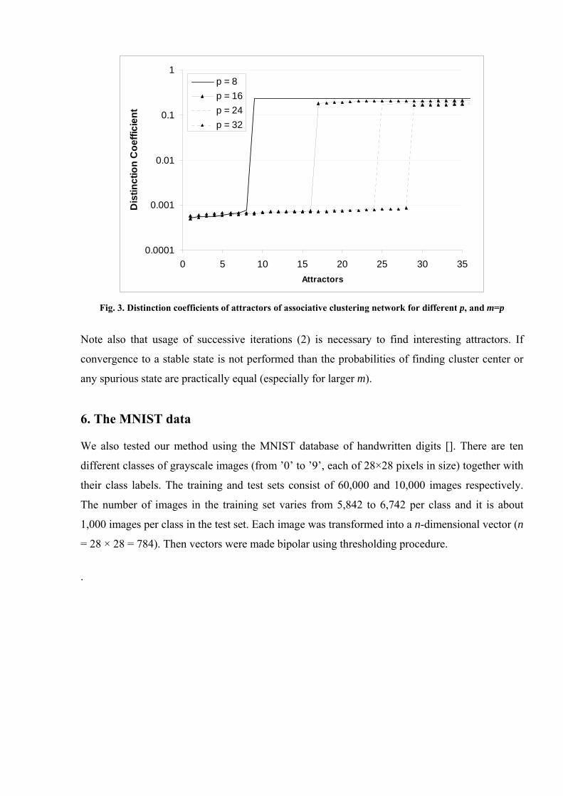
Figure 3 demonstrates another way of selecting attractors; here they are sorted by distinction

coefficient r(x,X) (3) with network’s synaptic matrix. Results of this experiments show that

difference of this measure between centers and spurious attractors is much stronger than for

frequencies. This ratio is almost the same for different network configurations. So, the

distinction coefficient might be used to reveal centers efficiently. Unfortunately, usage of this

criterion combining with random starts cannot guarantee that number of network runs was

sufficient to retrieve all centers. This can be seen from the results on fig. 3 for p = 32 – only 28

out of 32 centers were found using the value of distinction coefficient.

0.0001

0.001

0.01

0.1

1

0 5 10 15 20 25 30 35Attractors

Dis

tinct

ion

Coe

ffici

ent

p = 8p = 16p = 24p = 32

Fig. 3. Distinction coefficients of attractors of associative clustering network for different p, and m=p

Note also that usage of successive iterations (2) is necessary to find interesting attractors. If

convergence to a stable state is not performed than the probabilities of finding cluster center or

any spurious state are practically equal (especially for larger m).

6. The MNIST data We also tested our method using the MNIST database of handwritten digits []. There are ten

different classes of grayscale images (from ’0’ to ’9’, each of 28×28 pixels in size) together with

their class labels. The training and test sets consist of 60,000 and 10,000 images respectively.

The number of images in the training set varies from 5,842 to 6,742 per class and it is about

1,000 images per class in the test set. Each image was transformed into a n-dimensional vector (n

= 28 × 28 = 784). Then vectors were made bipolar using thresholding procedure.

.

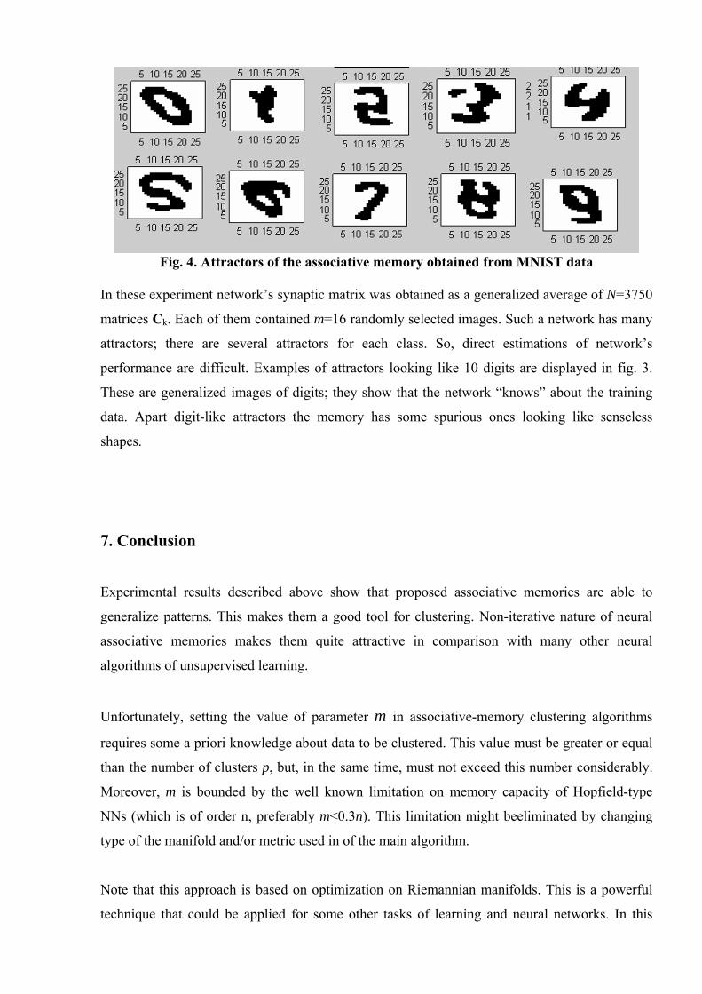
Fig. 4. Attractors of the associative memory obtained from MNIST data

In these experiment network’s synaptic matrix was obtained as a generalized average of N=3750

matrices Ck. Each of them contained m=16 randomly selected images. Such a network has many

attractors; there are several attractors for each class. So, direct estimations of network’s

performance are difficult. Examples of attractors looking like 10 digits are displayed in fig. 3.

These are generalized images of digits; they show that the network “knows” about the training

data. Apart digit-like attractors the memory has some spurious ones looking like senseless

shapes.

7. Conclusion

Experimental results described above show that proposed associative memories are able to

generalize patterns. This makes them a good tool for clustering. Non-iterative nature of neural

associative memories makes them quite attractive in comparison with many other neural

algorithms of unsupervised learning.

Unfortunately, setting the value of parameter m in associative-memory clustering algorithms

requires some a priori knowledge about data to be clustered. This value must be greater or equal

than the number of clusters p, but, in the same time, must not exceed this number considerably.

Moreover, m is bounded by the well known limitation on memory capacity of Hopfield-type

NNs (which is of order n, preferably m<0.3n). This limitation might beeliminated by changing

type of the manifold and/or metric used in of the main algorithm.

Note that this approach is based on optimization on Riemannian manifolds. This is a powerful

technique that could be applied for some other tasks of learning and neural networks. In this

paper we used specific manifolds (Grassmann). For this manifold we selected only one type of

distance (based on the Frobenius norm) and averaging. Moreover, the solution of corresponding

optimization task was not exact. We expect that usage of different metric combining with exact

geometric optimization may yield better performance of the associative-memory clustering.

Development of appropriate techniques of high-dimensional optimization is a subject of the

future work.

The proposed method may also be generalized for wider class of manifolds. In this case we

should use geometric computation that works for arbitrary manifold (e.g. described in [10]). This

extension of associative-clustering technique will enable to solve wider class of tasks.

References

1. L. Personnaz, I. Guyon, G. Dreyfus, “Collective computational properties of neural

networks: New learning mechanisms,” Phys. Rev. A, Vol.34 (5), pp. 4217-4228, 1986

2. Reznik A.M Non-Iterative Learning for Neural Networks. Proceedings of the

International Joint Conference on Neural Networks. (Washington DC), July 10-16, 1999

3. A.S. Sitchov. Methods of Improvement of Neural Associative Memory and its Application

to Hybrid Modular Neural Networks. Ph. D. thesis, IMMSP of NAS of Ukraine, Kyiv,

Ukraine 2003 (in Ukrainian)

4. P.-A. Absil, R. Mahony, R. Sepulchre. Riemannian geometry of Grassmann manifolds

with a view on algorithmic computation, Acta Applicandae Mathematicae, Vol. 80, No

2, pp. 199–220, Jan. 2004

5. A. Edelman, T. Arias, and S. Smith. The Geometry of Algorithms with Orthogonality

Constraints. Siam J. Matrix Anal. Appl. Vol. 20, No. 2, pp. 303-353

6. S.T. Smith. Geometric Optimization Methods for Adaptive Filtering. Ph.D. Thesis .

Harvard Univ. Cambridge MA, 1993

7. S.T. Smith. Intrinsic Cramer-Rao bounds and subspace estimation accuracy., 2004

8. Kohonen, Teuvo Self-organizing maps. Third edition. Springer Series in Information

Sciences, 30. Springer-Verlag Berlin, 2001.

9. A. Albert, Regression and the Moore-Penrose pseudoinverse, Academic Press, New

York-London, 1972

10. J.-P. Dedieu, D. Nowicki, Symplectic Methods for the Approximation of the Exponential

Map and the Newton Iteration on Riemannian Submanifolds. Submitted to the Journal of

Complexity (2004)

Chapter 3

Kernel-Based Associative Memory*

Dimitri Nowicki Institute of Mathematical

Machines and Systems of NASU Kiev, Ukraine

E-mail: nowicki@fromru.com

Oleksiy Dekhtyarenko Institute of Mathematical

Machines and Systems of NASU Kiev, Ukraine

E-mail: olexii@mail.ru

Abstract– We propose a new approach to pseudo-inverse associative memories using kernel machine methodology. Basing on Hopfield-type pseudoinverse associative memories we developed a series of kernel-based hetero- and auto-associative algorithms. There are convergence processes possible during examination procedures even for continuous data. Kernel approach enables to overcome capacity limitations inherent to Hopfield-type networks. Memory capacity virtually does not depend on data dimension. We provide theoretical investigation for proposed methods and prove its attraction properties. Also we have experimentally tested them for tasks of classification and associative retrieval.

I. INTRODUCTION

Nowadays there is a drastic growth in the domain of kernel machines. These methods and techniques are widely applied for pattern recognition, regression, classification and clustering. All kernel methods use feature space whose dimension is significantly larger than the dimension of original space. Original and feature spaces are connected by the nonlinear mapping:

.: XX EE ′→ϕ

Dimensionality of E'X might be very large or even infinite. So it is difficult or impossible to operate with vectors in this space explicitly. However sometimes one needs to know only inner (scalar) product in E'X as a function of elements of EX. This function is called kernel:

))(),((),( vuvuK ϕϕ= (1)

Most of kernel methods like SVM [1], LS-SVM [2] are used for classification, regression, and pattern recognition. Thus it will be interesting to construct kernel machines with other functions such as associative recall. The aim of this paper is to construct associative memory (AM) based on kernel machine.

Linear independence of memorized vectors is required by Hopfield-type associative memories. Moreover, their linear independence must be “sufficiently strong” i.e. every vector must be sufficiently far from the linear hull of all remaining ones. It implies that the *This research was supported by INTAS grant #01-0257

number of patterns to memorize must be less than their dimension. In practice this number does not exceed 25% (pseudoinverse learning rule, [3]) or 70% of vectors’ dimension (desaturation technique, see [4]). Diagonal elements of the synaptic matrix dominate if the number of patterns is close to this limit. This implies drastic decrease of attraction properties and deterioration of associative memory’s capabilities.

Using kernel machines one can change over to the space where memorized data set becomes linearly independent. We use pseudoinverse hetero- and auto-associative memory as a prototype. Usage of kernel machines in scope of this paradigm enables to overcome limitations due to linearity of the basic model. In particular, we can remove capacity limitations of these memories. Using this approach we also constructed associative memory capable to iterative convergence during examination process with the continuous data.

II. THE ALGORITHM

Lets consider pseudoinverse heteroassociative memory. Suppose EX and EX are input and output spaces with dimensionalities n and p respectively. We should store m pairs of vectors miEyEx YiXi Κ1,, =∈∈ . These vectors are supposed to form columns of matrices X and Y respectively. In order to provide appropriate heteroassociative behavior matrix B can be specified as:

YBX= whose solution is:

+= YXB (2)

This matrix defines a projective operator

YX EE →:B such that ii yBx = for all i. We denote by operator “+” the Moore-Penrose pseudoinverse of X (see e.g. [5]). In case of linearly independent columns pseudoinverse matrix can be found as

.)( 11 TTT XSXXXX −−+ == (3)

The elements of m×m-sized matrix S are computed as pairwise scalar products of memorized vectors:

).,( jiij xxs = (4)

Examination procedure takes an arbitrary input vector x. We should produce network’s response y. This cold be done as follows:

).,(;

;1

xxxXz

zYSB

ii

T

z

xy

==

== −

(5)

Note that we need to know only scalar products of memorized vectors themselves and input vector x.

We use this property of heteroassociative memory to construct the kernel algorithm. We replace EX by E'X whose dimensionality is nn >>′ (E'X may also be an infinite-dimensional Hilbert space). Vectors in E'X are evaluated using nonlinear transformation XX EE ′→ϕ : . E'X is called feature space.

Let Xiii Exxx ∈= ),(' ϕ be input vectors of training dataset, and ))(),((),( vuvu ϕϕ=K be a kernel.

Then, like (3-5) we get:

).,(

);,(

xxKz

xxKs

ii

jiij

=

= (6)

Expressions (2-3, 5-6) could be evaluated by means of kernel only, without explicit usage of E'X , this leading to kernel-based procedures of learning and examination.

This is a basic algorithm for kernel associative memory.

Corollary 1 of Mercer’s theorem: If K(u,v) is a Mercer’s kernel [1] then

1) Hilbert space E'X and a mapping XX EE ′→:ϕ exist such that ))(),((),( vuvuK ϕϕ=

2) For each set of pairs miEyEx YiXi Κ1,, =∈∈ matrix S is nonnegative-defined

3) If in addition dim(Ex')>m, there exists a operator YX EEB →′: such that ii yBx =' for all i.

Proof: 1) follows directly from Mercer’s theorem 2) this is true because the matrix S consists of

pairwise scalar products of Xi Ex ′∈′ (it is a Gram matrix of this set of vectors)

3) such an operator could be built on the

(m-dimensional) linear hull of Xmii E ′∈>′< =1x

and extended continuously to the whole E′x. Mercer’s condition is formulated as follows. Let

ℜ→×QQK :),( vu be a continuous symmetric function and Q be a compact set in Ex. Then, a space E'x and a mapping XX EE ′→:ϕ such that

xEX KEQvu′

=⊂∈∀ )(),(),(, vuvu ϕϕ exist if and only

if for any )(2 QLg ∈ following inequality holds:

0)()(),(,

≥∫∫∈

vgugvuKQvu

Unfortunately, we cannot guarantee non-singularity

of the matrix S. It is invertible if Xmii Ex ′∈>′< =1 are

linearly independent. This condition may not hold for certain kernels and specific vector sets. In practice, one can suppress this problem using Tikhonov’s regularization: instead of S using the matrix:

ISS µµ +=

for small µ>0. This matrix is always invertible since S is nonnegative definite.

Another approach to this problem uses incremental construction of the matrix S. During each step of the algorithm its dimensionality is increased by one with the addition of each next memorized vector. If this leads to singular matrix, the vector is rejected. For inversion of S we use the technique for block matrices [5,6].

To memorize m patterns in this network we need to store m×m-sized matrix S. We can say that kernel associative memory is capable to store as many images as neurons it has. This is a maximum estimation which is sometimes unreachable in practice. For instance, in case of scalar-product kernel this machine is identical to conventional neural heteroassociative memory.

III. MODIFICATIONS OF THE KERNEL ALGORITHM

A. Autoassociative memory

The algorithm described above might be also used for autoassociative memory. In this case Ex and Ey are identical, miyxEyEx iiYiXi Κ1,,, ==∈∈ . Matrix S is calculated by formula (6). There is an iterative examination procedure: the vector xt is sent to the network’s input, using (5-6) we obtain postsynaptic potential yt. Then, in case of bipolar data we apply activation function and compute the next state of the system:

)(1 tt yfx =+ (7)

This procedure is iterated until a stable state (attractor) has been reached. Attractors of such systems are described by

Theorem 1. Suppose for autoassociative memory (4-8) conditions of the corollary 1 hold, and matrix S is invertible. Then attractors of corresponding examination procedure are only fixed points or 2-cycles

Proof: We construct energy function in the way similar to the corresponding proof for Hopfield networks:

),(21- ttt yxKE = (8)

By corollary from Mercer’s theorem a self-conjugated operator yx EEC →′: exists such that Cx't=yt. Applying properties of scalar product in E'x we get:

( ) ( )

( ) ( )

),(21),(

21

','21','

21

','21','

21

11

11

111

−+

+−

+−+

−=

=+−

=+−=−

tttt

tttt

tttttt

xyKxyK

CxxCxx

CxxCxxEE (9)

Since the kernel is monotonic function with respect to distance between x and y expression (9) is non-negative, it is zero if and only if the fixed point is reached.

The scheme of examination algorithm for auto-associative memory is displayed in the fig. 1.

Fig. 1. Scheme of the kernel autoassociative memory

B. Internal activation function

Consider the vector zSw 1−= . It corresponds exactly to k-th memorized pattern if and only if ikiw δ= . To provide a better convergence to such w we apply internal activation function:

)(: iwwF θ=′′→ ww where ]1,0[]1,0[: →θ is smooth monotonic function such that 0)1()0(;1)1(,0)0( =′=′== θθθθ .

IV. EXPERIMENTAL RESULTS Our models and algorithms were experimentally

tested for several tasks of auto- and heteroassociative recall and classification. Here we display results or auto-associative memory working with simulated data arrays

and real-world data (images). For experiments we used following three types of kernel:

1. Polynomial

( )integer positive,0

,),(1),(−>

+=βα

α βyxyxK (10)

2. Gaussian RBF ( ) 0,exp),( 2 >−−= αα yxyxK (11)

3. Power RBF:

( ) 0,0,1),( 2 >>−+= βααβ

yxyxK (12)

We studied attraction properties of kernel associative memory. All experiments were performed using internal activation function and iterative examination procedure. Algorithms were implemented using neural-network software package NeuroLand [7].

Gaussian kernel

0

5

10

15

20

1.0E-04 1.0E-03 1.0E-02 1.0E-01 1.0E+00 1.0E+01 1.0E+02

alpha

Attr

actio

n ra

dius

(%)

RBF kernel

0

2

4

6

8

10

12

1.E-07 1.E-05 1.E-03 1.E-01 1.E+01 1.E+03alpha

Attr

actio

n ra

dius

(%)

beta = -1

beta = 2

Polynomial kernel

0

5

10

15

20

1.E-06 1.E-04 1.E-02 1.E+00 1.E+02alpha

Attr

actio

n ra

dius

(%)

beta = 4

beta = -4

Fig. 2. Attraction radius of kernel AM for bipolar data

A. Simulated bipolar data

To study attraction properties of kernel associative memory for bipolar data we choose a network memorizing 264 64-dimensional patterns. Bipolar data

vectors were randomly generated, probabilities of values +1 and -1 for each component were equal, and components were independent.

Attraction radius was measured as a maximum value of bipolar noise such that the network still gave correct responses for all memorized patterns. In fig. 2 we display attraction radius depending on parameters for kernels (10-12).

B. Image data

In these experiments we used 30×30 gray-scale photographs of faces. They were presented as real-valued vectors with components normalized to [-1;1], the kernel AM memorized 61 images.

Gaussian kernel

0

0.5

1

1.5

2

2.5

0 0.01 0.02 0.03 0.04 0.05

alpha

Attra

ctio

n ra

dius

RBF kernel, beta = -1

0

0.2

0.4

0.6

0.8

1

1.E-08 1.E-07 1.E-06 1.E-05 1.E-04 1.E-03 1.E-02 1.E-01 1.E+00

aplha

Attr

actio

n ra

dius

Polynomial kernel

0

0.5

1

1.5

2

1.E-08 1.E-07 1.E-06 1.E-05 1.E-04 1.E-03 1.E-02 1.E-01 1.E+00aplha

Attr

actio

n ra

dius

beta = 4

beta = 8

Fig. 3. Attraction radius of kernel AM for picture data

Input vectors were obtained from original patterns by adding Gaussian noise with zero mean. Standard deviation σ of this noise served as a measure of attraction radius. More precisely, attraction radius was set equal to σ such that all images were restored with fixed precision ε. Attraction radius depending on parameters for kernels (10-12) is displayed in fig. 3.

V. CONCLUSION This article introduces associative memory based on

kernel machine. We present theoretical justification and experimental tests for these techniques.

Unlike [8], where author uses high order generalization of the Hopfield model that includes interactions between more than two neurons, we restrict ourselves to two component Hamiltonian (energy function). Doing so we are able to provide analytical solution for the stability equation (2).

Experimental results show that proposed kernel algorithm successfully works as auto- and heteroassociative memory. We demonstrate attraction properties of kernel AM for different types of data. It may also be used for classification and pattern recognition. Using kernel methods we can construct iterative examination procedure even for continuous data. Also we can increase capacity of associative memory and overcome limitations inherent to Hopfield-type neural networks.

REFERENCES [1] V. Vapnik, Statistical Learning Theory, John Wiley & Sons, NY,

1998. [2] Smale S. On the Mathematical Foundations of Learning Bull. Am.

Math. Soc., Vol. 39, No. 1, pp. 1-49, 2001. [3] L. Personnaz, I. Guyon, G. Dreyfus, “Collective computational

properties of neural networks: New learning mechanisms,” Phys. Rev. A, Vol.34 (5), pp. 4217-4228, 1986.

[4] D.O. Gorodnichy, A.M. Reznik, “Increasing Attraction of Pseudo-Inverse Neural Networks,” Neural Processing Letters, vol. 5, pp. 121-125, 1997.

[5] A. Albert, Regression and the Moore-Penrose pseudoinverse, Academic Press, New York-London, 1972.

[6] L.A. Pipes, Applied mathematics for engineers and physicists, McGraw-Hill Book Co., New York-Toronto-London, 1958.

[7] A.M. Reznik, E.A. Kalina, A.S. Sitchov, E.G. Sadovaya, O.K. Dekhtyarenko, A.A. Galinskaya, “The multifunctional neural computer NeuroLand,” Proceedings of the Int. Conf. on Inductive Simulation, Lviv, Ukraine, vol.1 (4), pp. 82-88. May 20-25, 2002.

[8] Barbara Caputo, “Storage Capacity of Kernel Associative Memories,” Proceedings of the Int. Conf. on Art. Neural Networks, Aug. 27-31 2002, Madrid, Spain.

Associative Memories with "Killed" Neurons: the Methods of Recovery*

A.M. Reznik, A.S. Sitchov, O.K. Dekhtyarenko, and D.W. Nowicki The Institute of the Mathematical Machines and Systems, Ukrainian National Academy of Science

03187, 42 Glushkov Str, Kiev, Ukraine neuro@immsp.kiev.ua

Abstract–We consider re-learning ability of a Hopfield-type network after killing some neurons. Neurons were "killed" by means of nullification of corresponding rows and columns of the synaptic matrix. We show that one can restore recognition ability of this network using re-training with the vectors, which were memorized before. The number of vectors needed is equal to the number of deleted neurons. It does not depend on network's size and on volume of stored data.

INTRODUCTION

It is known that a classical Hopfield network has decreasing convergence ability with respect to number of memorized vectors. Such a network cannot store more vectors than 14% of neurons' number [1]. Pseudoinverse learning rule enables to increase this ratio up to 25% [2]. In this case we must to store exact weight values in the synaptic matrix (at least 7 bits per weight, [3]). But sometimes disturbance of accurate weight values does not decreases convergence ability of the Hopfield-type network. On the contrary, some distortions may make it work better as an associative memory. Let us note some examples of such "useful distortions": methods of desaturation [4], which allows increasing of the memorize ability about 5 times, pseudoinverse adaptive filter [5], method of weight selection (it enables to reduce number of weights to 30% of original quantity not worsening associative-memory capabilities, [6]). These examples illustrate the effect of information redundancy inherent to Hopfield-type associative memories

Therefore the following question seems to be interesting: Does the redundancy effect work if some neurons of the Hopfield-type network are completely destroyed? Could one recover the associative memory in this case? To answer these questions we consider a pseudo-inverse network with some neurons "killed" by means of nullification of all their synaptic weights (both for the inputs and the outputs). Once exposed to such a distortion, the network loses its ability to converge, i.e. the destruction of associative memory takes place and all its content becomes inaccessible. We show that it is possible to recover the network completely via retraining it with some of the previously stored vectors. The number of vectors needed is equal to the number of deleted neurons. It does not depend on network's size and on volume of stored data. This phenomenon looks like recovery of amnesia patients after reminding them significant events of their past.

*This research was supported by INTAS-01-0257

THE MODEL OF NEURAL NETWORK

According to the J. Hopfield’s scheme each neuron is connected to each other and itself; forward and backward connections have the same weight. Weighted sum of output signals forms a postsynaptic potential (PSP). Depending on a sign of this sum the neuron's output possess the values +1 or -1. The outputs form a N-dimensional vector of current network's state, and weights form a synaptic matrix C. Under certain conditions for this matrix the network has stable states called attractors. If a network state isn't an attractor the process of convergence will take place. Convergence ends in a nearest attractor. The convergence process looks like an associative recall, that's why networks of this type are known as associative memories. The algorithm for calculation of synaptic matrix from given set of attractors [2] is based on solution of the stable state equation:

CU = U. (1)

Here U is a matrix M × N. The vectors of desired attractor

states are its columns. The solution of this equation has a form:

C = UU+, (2)

Besides the main attractors defined by equation (1) the

network has spurious equilibria defined as solutions of non-linear stability equation.

If there are many spurious attractors the network may stop at them before converging to main attractors. Spurious attractors exert influence only if M/N > 1/10. For slightly saturated networks they could be neglected. The pseudoinverse algorithm is commonly used to compute value of the matrix C. It enables to successively update the matrix in memorizing of each vector from U [4].

Cm= Cm-1 + ∆m;

∆M= (I- Cm-1)UUT(I- Cm-1)/ UT(I- Cm-1)U, (3)

where Cm is a value of synaptic matrix after memorizing M vectors.

An expression for ∆m could be rewritten in the form:

∆ijM = (ui - si) (uj - sj)/q, (4)

0-7803-7898-9/03/$17.00 ©2003 IEEE 2579

where is a postsynaptic potential of

j-th neuron; q

∑ == N

j jiji uCs1

∑=

−=N

jj su

1( jj u)

A normed value of q is called coefficient of distinction. It describes a component of vector U orthogonal to m-1 previously stored vectors.

k = q /N. (5)

The value of k decreases as U approaches to linear hull of Ui and reaches zero when U belongs to this linear hull. Such a behavior resembles the resonance effect as it emphasizes the difference between similar stored vectors.

Quality of associative memories could be also described in terms of attraction radius. Direct attraction radius is the largest value of Hamming distance between initial point and the attractor for that the examination procedure starting at this point will still converge to the corresponding attractor during one iteration.

The value of direct attraction radius depends on data nature and could be estimated by the following expression [4]:

1])/(/][/)1(1[)1(5.0 5,025,0 +−+−−< −NMNMNMNH α (6)

A positive value α<1 is called desaturation coefficient. Diagonal terms of the matrix should be multiplied by this value to fasten convergence and to resist saturation effects.

During experimentation we use the concept of the full attraction radius, which is the maximum Hamming distance covered by the network as it reaches the state of attraction (regardless of the number of iterations). The full attraction radius normally is 3-5 times greater than attraction radius given by (6) and is more important for the practical applications.

CHANGE OF ATTRACTION PROPERTIES AFTER REMOVING CONNECTIONS

Partial removal of connections causes change of the PSP.

Small changes do not affect its sign; so they don't cause network's state changes. In this case the effect could be seen due to change of the distinction coefficient. This coefficient describes network's behavior in the neighborhood of the attractor.

The histograms of k are for the network of 256 neurons displayed in the fig. 1. In this network all connections of n (randomly selected) neurons were destroyed after memorizing M vectors. For these experiments the NeuroLand software package [6] was used. Memorized and test vectors were generated randomly. We can see that the distribution of k looks like normal. The removal of just 10% of neurons leads to the significant non-zero k values that signifies the loss of the synaptic matrix projective properties and the deterioration of the network recall capacities.

00.05

0.10.15

0.20.25

0.30.35

0.40.45

0.122 0.162 0.202 0.242 0.282 0.322 0.362 0.402 0.442 0.482

distinction

M/N %"killed" %

5%10%

25%10%50%

10%50%30%

25%30%

5%30%

Fig. 1. The k value distinction for various memory saturations (M/N) and “killed” neuron portions.

TRAINING DISTORTED NEURAL NETWORK

In the fig. 1 we can see resonance properties of the NN changed. These changes increase a probability of stop in the spurious attractors. So the volume of data recalled is decreased. Moreover, loss of projectivity of the synaptic matrix may damage memorizing recall abilities more seriously. If one uses formulae (3, 4) to correct perturbed matrix then distortion will be only cumulated. That does finally completely destroy the associative memory. To verify these assumptions we have made some experiments. Under certain conditions the results were completely opposite.

The results for memorizing 120 vectors and “killing” 40 neurons in the network of 256 neurons are presented in the figs. 2 and 3. For examination we used desaturation with α = 0.1. According to formula (6) H = 8.7, and the complete attraction radius was about 35. To obtain the AR experimentally we use noisy values of stored vectors as initial conditions for the convergence process. Complete attraction radius was defined as a maximum value of H for that network was converged to the correct image for 95 of 100 noise instances.

Data for “killing” 40 neurons and re-memorizing 10, 30, and 40 vectors are displayed in the fig. 2, 3. Vectors for retrain were randomly selected from images initially stored. Fig 2 depicts the values of attraction radius for the remaining part of the network (216 neurons).

We can see that the destroyed network completely losses its convergence ability. Only for one of 120 initially stored images (#100) attraction radius was non-zero. During additional training attraction radius is recovered completely for retrain images and partially fore the rest. As number of retrain vectors gets equal to number of “killed” neurons attraction properties of the network are completely restored. The distinction coefficient with respect to retrain dynamics is shown the figure 3. Unlike fig. 2 this graph takes into account all 256 neurons of the network. Dynamics of k with respect to retrain looks like attraction radius dependencies. After re-memorizing 40 vectors it turns to zero for all stored images.

The recovery effect for associative memories takes place if

2580

020

4060

80100

erased10th retrain

30th retrain40th retrain

0102030

40

50

H

stored vectors

Fig. 2. The changes of attraction radius with net retrain.

020 40 60 80 100

40th retrain30th retrain

10th retrainerased

0

0.05

0.1

0.15

0.2

k

stored vectors

Fig. 3. The changes of distinction coefficient with net retrain

05

101520253035404550

0 10 20 30 40 50 60 70 80 90 100 110 120 130

stored vectors

attra

ctio

n ra

dius

with retrainwithout retrain

Fig. 4. The change of attraction radius with net extra train

and only if retrain data belongs to a set of initial images. If we take different vectors attraction abilities of the network could not be restored. That follows from fig. 4: attraction radius after storing 15 new vectors in the network. These are vectors #121 and more. The dependencies for new training that is done immediately after killing 40 neurons (bold line) or following retraining (thin line) are displayed in this graph. We can see that without retraining attraction radius is zero for all previously stored vectors. For the new stored vectors attraction radius (it was more than 40) increases in comparison with the value before damaging network. It could be explained by the fact that the trace of the synaptic matrix was decreased by the neurons removal, thus the sum of

eigenvalues defining the associative memory saturation became smaller.

SPECTRA OF DISTORTED SYNAPTIC MATRICES

The recovery process of associative memory could be

observed by examining spectra of synaptic matrices. Data for the matrix 256×256 with 120 stored vectors after nullification of 40 rows and columns are displayed in fig 5. There are graphs of sorted spectra before retraining and after 10, 30, and 40 retrain vectors. We can see that "killing" neurons preserves rank of the matrix, although values of 40 eigenvalues of 120 strongly decreased. After storing each following vector rank of the matrix increases by one, an eigenvector with value of 1 is added, 40 weakened eigenvalues are changing. After retrain they form a tail of the spectrum; these eigenvalues are less than 0.47. There is an orthogonal component with respect to original memorized vectors in eigenvectors of the corrupted matrix. Fig. 5 displays data for dense filling of the memory (M/N>=0.47) after removal of 15% of neurons. Fig. 6 displays data for slight filling of the same network (M/N>=0.15) after removal of 10 neurons only. There are spectra before retraining, after 5 and 10 retrain vectors and after additional training with 20 new vectors.

0 40 80 120160

200240

erased10th retrain30th retrain40th retrain0

0.2

0.4

0.6

0.8

1

eigenvectors

Fig. 5. Spectra evolution during the net retrain (M = 120)

0 10 20 30 40 50 60 70erased

5th retrain10th retrain

20th new train0

0.2

0.4

0.6

0.8

1

eigenvectors

Fig. 6. Spectra evolution during net retrain and extra train with new data (M = 40+20)

2581

Note that 20 new eigenvectors with λ = 1 almost do not influence on 10 small eigenvalues (appeared after corruption).

For slightly saturated memory non-projectivity of the matrix does not practically influence on the network's behavior. However for strongly filled memory there are many spurious attractors; so, available associative memory is reduced. We can depress spurious attractors using desaturation. To reduce non-projectivity more drastically one could raise the synaptic matrix to high power; so only eigenvalues close to 1 would be preserved.

CONCLUSION

Considering the results of our experiments it is worth to emphasize that the discussed phenomenon covers not only a simple substitution of “killed” neurons and their connections, but also the complete recovery of the autoassociative memory functions for the remaining part of the net (its functionality was lost due to the loss of the network ability to converge towards attractors). Therefore it is possible to say about the recovery both of stored data and the autoassociative access mechanism.

We have done experiments on network recovery for Hopfield-type networks with 64 to 2048 neurons for different levels of saturation and corruption. In all the case the network could be completely recovered using retraining with original data.

The number of retrained images needed for the complete recovery was always equal to the number of deleted neurons. We have not revealed any differences caused by the various possible selections of retrained images from the already stored ones in the network. Such independence on the retrain set selection could be used for designing of ultra stable systems that are capable to preserve their features in spite of constant resource degradation. In order to achieve it, these systems must undergo recovery via retraining of a control dataset more intensively than the resource degradation occurs.

This phenomenon looks like recovery of amnesia patients

after reminding them significant events of their past. So, we can make the conjecture that in the biological neural systems there are mechanisms working like pseudo-inverse associative memories. We can cite some facts of biological neuroscience to support this conjecture. Not that most nerve fibers are less than 2 mm long; size of the dendrite branching area (0.1-0.4 mm) has the same order. In 1 mm2 there are thousands strongly connected neurons. So, they form local structures of 100-1000 neurons looking like Hopfield-type networks. We can suppose that these structures perform information memorizing and retrieval. In scope of our model and results long-term memory acts by systematic reactivation of local structures; they are re-training with previously memorized patterns. Memory corruption is prevented due to continuous conscious and subconscious work of the brain; also due to the dream activity. The further research in cooperation with specialists in biological neuroscience and psychologists is needed to verify these conjectures.

REFERENCES [1] J.J. Hopfield, “Neural networks and physical systems with emergent

collective computational abilities,” in Proc. Nat. Acad. Sci., vol. 79, pp. 2554-2558, Apr. 1982.

[2] L. Personnaz, I. Guyon, G. Dreyfus, “Collective computational properties of neural networks: New learning mechanisms,” Phys. Rev. A., vol. 34, no. 5, pp. 4217-4228, 1986.

[3] M. Weinfield, “A fully digital integrated CMOS Hopfield network including learning algorithm,” in Proc. Int. Workshop WLSI Art. Intell., Univ. of Oxford, E1-E10, 1988.

[4] A.M. Reznik, D.O. Gorodnichy, A.S. Sitchov, “Regulating feedback bond in neural networks with learning projectional algorithm,” Cybernetics and system analysis, vol. 32, no. 6, pp. 868-875, 1996.

[5] A.M Reznik, "Non-iterative learning for neural networks," in Proc. Int. Joint Conf. Neural Networks, Washington, no. 548, July, 1999.

[6] A.S. Sitchov, “Weight selection in neural networks with pseudoinverse learning rule,” (in Russian) Mathematical Machines and Systems, vol.2, pp. 25-30, 1998.

[7] A. M. Reznik, E.A. Kalina, A.S. Sitchov, E.G. Sadovaya, O.K. Dekhtyarenko, A.A. Galinskaya, “Multifunctional neurocomputer NeuroLand,” (in Russian) in Proc. Int. Conf. Inductive Simulation, Lviv, Ukraine, vol. 1(4), pp. 82-88, May 2002.

2582

Chapter 4

1

Filtering of Deep Brain Stimulation Artifacts out Using a Nonlinear Oscillatory Model

Aksenova T.I.1,2, Nowicki D.V.*1,3, Benabid A-L1

1 Unit 318, INSERM CHU A. Michallon, BP 217, 38043 Grenoble, Cedex 09, France

2 Institute of Applied System Analysis, Ukrainian Academy of Sciences, Prospekt Peremogy, 37, Kiev 03056, Ukraine

3Institute of Mathematical Machines and Systems 42 Glushkov ave., 03187 Kiev Ukraine

E-mail:

tatyana.aksyonova@ujf-grenoble.fr nowicki@nnteam.org.ua

Alim-Louis.Benabid@ujf-grenoble.fr

ABSTRACT

The present paper is devoted to suppression of spurious signals (artifacts) in records of neural activity during deep brain stimulation.. An approach based on nonlinear adaptive model with self-oscillations is proposed. We developed an algorithm of adaptative filtering basing on this approach. The proposed algorithm was tested using records collected from patients during the stimulation. Then it was compared to existing methods, and showed the best performance.

1. Introduction

This paper presents an approach for filtering signals of neuronal activity during Deep Brain Stimulation (DBS) using nonlinear oscillatory models. High-frequency (100-300 Hz) DBS is a surgical procedure for treating a variety of disabling neurological symptoms, in particular due to Parkinson’s disease. In spite of its clinical efficiency over 20 years the mechanism of action of DBS is still a matter of debate (Benabid et al, 2005; McIntyre CC et all, 2004). Understanding how DBS at high frequency works is of paramount importance as this will provide the understanding of the circuitry of basal ganglia. The major difficulty of to study the mechanism of action of DBS is that the appropriate signal of neuronal activity during the stimulation, namely the extracellular microelectrode recording of action potentials (spikes), cannot be analyzed directly due to stimulation artifacts present in the records (Fig. 1a, 2a). The artifacts are induced by the periodically repeated electrical impulses delivered to the target zone in the brain. The artifacts have a common waveform but are not identical due sampling errors and irregularities of stimulus production. The Artifact-to-Signal Ratio (ASR), which is the ratio of the mean of amplitudes of artifacts to the averaged amplitude of spikes of neuronal activity observed before the stimulation, varies between 5 to 20. Typical artifact duration in the timeline is 20-50% of each stimulation period (Fig. 3a) although the pulse width of the stimulating pulse (60µs) is less than 1%

* D.V. Nowicki is a corresponding author

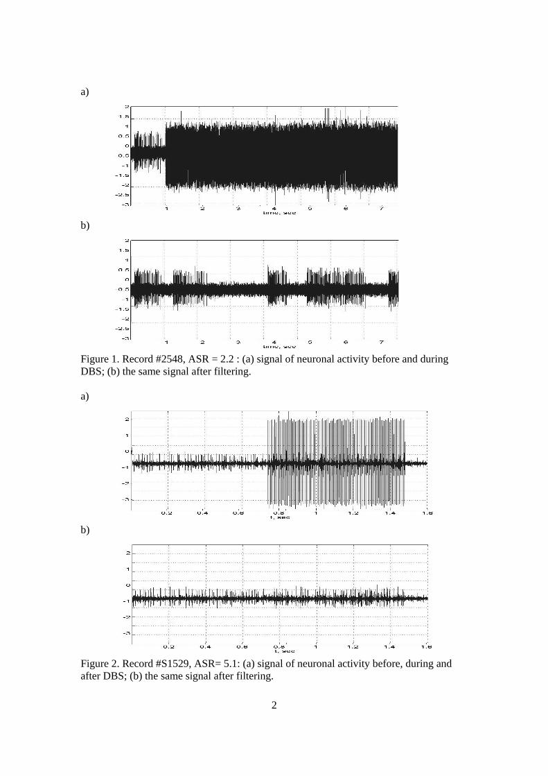
2

a)

b)

Figure 1. Record #2548, ASR = 2.2 : (a) signal of neuronal activity before and during DBS; (b) the same signal after filtering. a)

b)

Figure 2. Record #S1529, ASR= 5.1: (a) signal of neuronal activity before, during and after DBS; (b) the same signal after filtering.

3

There are several recent studies focused on removal, subtraction, or filtering of stimulation artifacts from electrophysiological signals: electroencephalogram (EEG), electromyograms (EMG), local field potentials (LFPs) and extracellular microelectrode recording of neuronal action potentials. Hardware techniques include hardware blanking (Robby&Lettich, 1975),(Knaflitz & Merletti, 1988) hardware filtering (Solomonow et al., 1985), varying amplifier gain (Roskar & Roskar, 1983) or their composition (Rossi et al., 2007). Algorithms of digital signal processing exploit several ideas. Time segments containing artifact peaks are cut off from the record at (O’Keeffee et al., 2001, Hines et al., 1996, etc.). An estimate the stimulus artefact waveform and subtracting from the signal is a basic idea of another group of algorithms. An efficiency of the use of software or hardware blanking depends on the assumption that the stimulus artefacts and the biopotentials are well separated in time domain. In the case of extracellular microelectrode recording of neuronal action potentials during High-frequency DBS these techniques lead to loss of substantial part of information because of artifact duration is 20-50% of stimulation period while stimulus artifacts and action potentials are overlapping in the time. The overlapping of the stimulus artefacts and action potentials in frequency domain (Wichmann, 2000) leads to the loss of high frequency components of extracellular microelectrode recording of neuronal action potentials in case of the use of band pass filters. To avoid the suppression of the high frequency components subtraction techniques were developed. However, most subtraction techniques suffer from an inability to adapt to the nonlinear dynamic of artefacts and hence suffer from the residual artefacts (O’Keeffee et al., 2001). Stimulus artifact suppression by subtraction of locally fitted polynomials is proposed in (Wagenaar & Potter, 2002). An advantage of this approach is that it doesn’t depend on the stability of stimulus artefact waveform. Each artefact is considered as independent. This method enables to reduce a time interval after stimulation when action potentials can not be detected to 2 ms. Nevertheless high frequency interval of stimulus artefact (about 25% of record time for DBS 130Hz) is lost. Estimates of representative stimulus artefact waveform was studied by Wichmann (2000). Template is generated by averaging a set of peri-stimulus segments adjusted by time shifting and scaling. Hashimoto et al. (2002) create several templates in order to account for artifact variability. Residual artefacts of 0.8-0.9 ms duration (Hashimoto et al (2002), and Tai et Al (2004)) are cut from the signal before further analysis. This part (about 11% of record time for DBS 130Hz) is no longer available for spike sorting, etc. Such a cut-off can still significantly corrupt spike trains obtained from the analyzed records. This paper presents an algorithm for filtering the signal of neuronal activity during DBS. It is based on the use of a nonlinear oscillation model to explain variability of the artefacts of stimulation and provides signal synchronization in phase space

4

a)

-4 -3 -2 -1 0 1 2 3 4-1

-0.8

-0.6

-0.4

-0.2

0

0.2

0.4

0.6

0.8

1

t, msec

b)

-4 -3 -2 -1 0 1 2 3 4

-0.3

-0.2

-0.1

0

0.1

0.2

0.3

t, msec c)

-4 -3 -2 -1 0 1 2 3 4

-0.25

-0.2

-0.15

-0.1

-0.05

0

0.05

0.1

0.15

0.2

0.25

t, msec Figure 3. Signal #S1529, ASR= 5.1 sliced into the stimulation-period windows (a) before filtering; (b) after filtering based on the model with additive noise; (c) after filtering according to phase-space algorithm. 2. Methods 2.1. Signal Characteristics The following indices of original and processed signal are used. Artifact level AL is a mean of maximal (original or processed) signal absolute values, such maxima were taken across artifact peaks. Spike level (SL) is a mean of maxima taken in spikes with no stimulation. Confidence interval (at confidence level 0.95) in assumption of Gaussian distribution of noise was used to estimate Noise level. The centered signal of neuronal activity observed before stimulation was used for its estimation. Because of presence of outliers in the data due to spikes, confidence intervals were estimated using median

5

absolute deviation MD. In case of normal distribution, the (theoretical) standard deviation σ and the absolute median deviation μ are linked via equation:

21

22)Pr(

0

2 2

2

==≤ ∫−

dtettμσ

πμ

Solving this equation we obtain μ=aσ, where 67448975.0≈a . Therefore, for a given confidence level we can use an estimation NL≅ (1.959965/a)*MD. From these values ASR=AL/SL, artifact-noise ratio ANR=AL/NL, spike-noise ratio SNR= SL/NL were derived. 2.2. Modelling Basic methods (Hashimoto et al, 2002, 2003) treat artifacts as a periodic function with additive noise:

xSt (t + kT ) = xSt0 (t) +ξk (t), 0 < t ≤ T, (1)

where T is the period of stimulation; k is the number of stimuli; xSt0 (t) is the mean

stimulus; ξk (t) are independent random variables with zero mean and finite variance σξ

2 (t) . In this case, the mean artifact can be estimated by averaging the observed signals of stimulation. Subtracting this mean from the signal can achieve relatively rough signal cleaning. The results of filtering according to Eq.1 are presented in Fig. 3b. The signals presented as examples in the articles (Hashimoto et al, 2002, Tai et al, 2004) have an ASR approximately equal to 3 - 6. After template subtraction, they still contained artifact residuals 1.5-2 times greater than spikes. The quality of filtering is characterized also by the phase dependent standard deviations of the residuals STD(t), 0 < t ≤ T (Fig. 4). a)

b)

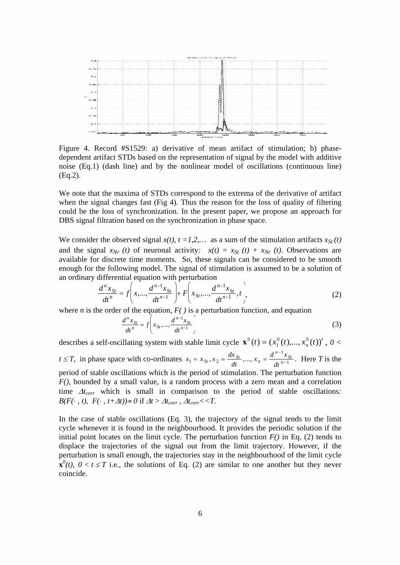
6

Figure 4. Record #S1529: a) derivative of mean artifact of stimulation; b) phase-dependent artifact STDs based on the representation of signal by the model with additive noise (Eq.1) (dash line) and by the nonlinear model of oscillations (continuous line) (Eq.2). We note that the maxima of STDs correspond to the extrema of the derivative of artifact when the signal changes fast (Fig 4). Thus the reason for the loss of quality of filtering could be the loss of synchronization. In the present paper, we propose an approach for DBS signal filtration based on the synchronization in phase space. We consider the observed signal x(t), t =1,2,… as a sum of the stimulation artifacts xSt (t) and the signal xNr (t) of neuronal activity: x(t) = xSt (t) + xNr (t). Observations are available for discrete time moments. So, these signals can be considered to be smooth enough for the following model. The signal of stimulation is assumed to be a solution of an ordinary differential equation with perturbation

d n xSt

dt n = f x,..., d n−1xSt

dt n−1

⎛

⎝ ⎜

⎞

⎠ ⎟ + F xSt ,...,

d n−1xSt

dt n−1 , t⎛

⎝ ⎜

⎞

⎠ ⎟ , (2)

where n is the order of the equation, F( ) is a perturbation function, and equation d n xSt

dt n = f xSt ,...,d n−1xSt

dt n−1

⎛

⎝ ⎜

⎞

⎠ ⎟ (3)

describes a self-oscillating system with stable limit cycle ))(),...,(()( 001

0 ′= txtxt nx , 0 <

t ≤ T, in phase space with co-ordinates x1 = x St , x 2 =dx St

dt, ..., x n =

d n −1x St

dt n −1 . Here T is the

period of stable oscillations which is the period of stimulation. The perturbation function F(), bounded by a small value, is a random process with a zero mean and a correlation time Δtcorr which is small in comparison to the period of stable oscillations: B(F(⋅ , t), F(⋅ , t+Δt))≈ 0 if Δt > Δtcorr , Δtcorr<<T. In the case of stable oscillations (Eq. 3), the trajectory of the signal tends to the limit cycle whenever it is found in the neighbourhood. It provides the periodic solution if the initial point locates on the limit cycle. The perturbation function F() in Eq. (2) tends to displace the trajectories of the signal out from the limit trajectory. However, if the perturbation is small enough, the trajectories stay in the neighbourhood of the limit cycle x0(t), 0 < t ≤ T i.e., the solutions of Eq. (2) are similar to one another but they never coincide.

7

Let us introduce the local coordinates in the neighbourhood of the limit cycle following Gudzenko (1962). Let us fix an arbitrary point on the limit cycle P0 as a starting point. The position of any arbitrary point P on the limit trajectory can be described by its phase θ, which is a time movement along the limit cycle from a starting point P0 , defined as P0 (θ = 0). Let us assume that function f() in Eq. (2,3) is twice continuously differentiable on all the arguments of the function, thus providing a necessary smoothness. At a point P with phase θ it is possible to construct a hyperplane (and only one such hyperplane) that is normal to the limit cycle. Let us consider an arbitrary trajectory Eq. (2) in the neighbourhood of the limit cycle. Denote M(θ ) the point of its intersection to the hyperplane of phase θ and set the point of phase zero M(0), θ = 0 as the initial point for analyzed trajectory. Any trajectory can be described by variables n(θ) and t(θ) (Fig. 5) where n(θ) is a vector of normal deviation defined by M(θ ) and its orthogonal projection P(θ ) on the limit cycle. The second variable t(θ) is a time movement along the trajectory from the initial point M(0) to the analyzed point M(θ ). Thus, the limit trajectory is defined by n(θ)≡ 0 and t(θ)≡θ, where 0 is a vector with all components equal to 0.

M: n(θ), t(θ)

P0

P(θ)

M0

n(θ)

Figure 5. The local coordinates in the neighbourhood of stable limit cycle. Let γ(θ) be the phase deviation, γ(θ) = t(θ)−θ. Eq. (2) could be rewritten in linear approximation (Gudzenko, 1962) in the deviations n(θ) and γ(θ) as follows:

n(θ ) dθ + N n[ ]= Fn (θ ) dγ dθ + (Θ ⋅ n) = Fγ (θ ) . (4)

Here N(θ) and Θ(θ) are the functions of the parameters. As a result the signal trajectory in phase space is presented in linear approximation as a sum of periodic components of limit cycle and function of deviation x(t(θ))=x0(θ) + n(θ), where n(θ) and t(θ)=γ(θ)-θ are following Eq.4. Thus, both models of the artifacts (Eq. 1 and Eq. 2) describe signals close to periodic ones. The model with additive noise (Eq. 1) explains the distortion of the amplitude of the signal only, while the model of nonlinear oscillations with perturbations (Eq. 2) explains the distortion of both amplitude and phase (Eq. 4). For the following artifact filtering, the limit cycle that presents a periodic component of signal should be estimated. The limit cycle is described as x0(θ), 0<θ ≤ T, phase running from 0 to T. Let us consider the segments of an arbitrary signal trajectory xi (t(θ)), 0<θ ≤

8

T with phase θ running from 0 to T, referred to as cycles. General population X = {xi (t(θ)), 0<θ ≤ T} is formed by cycles and corresponds to the realizations of the artifacts of stimulation. The limit trajectory x0(θ), 0 < θ ≤ T corresponds to an ideal “undisturbed artifact of stimulation”. The arbitrary cycle is presented as

xi(t(θ))=x0(θ) + ni(θ) , 0<θ ≤ T (5) where ni(θ) is determined by (Eq. 4). The mean trajectory converges to the limit cycle x0(θ) in linear approximation if the number of averaged trajectories increases infinitely (Gudzenko, 1962). It allows estimating the limit cycle x0(θ) by calculating the mean of the observed cycles xi (t(θ)), 0<θ ≤ T in the phase space.

˜ x 0 ( ˜ θ ) =1k

x i (t i (θ ))i=1

k

∑ , ˜ θ = 1k

ti (θ )i=1

k

∑ . (6)

Other statistics could be also used, taking into account that ni(θ) and γi(θ) are characterized by an asymptotically Gaussian distribution for any θ in the case of uncorrelated noise F() (Gudzenko 1962). After the estimation of the mean of the artifacts of stimulation ˜ x 0 ( ˜ θ ) in phase space, it is subtracted from the signal. For this purpose, local coordinates t i ( ˜ θ ) are calculated for each cycle. Then the functions of the vectors of normal deviations ni ( ˜ θ ) = x i (t i ( ˜ θ )) − ˜ x 0 ( ˜ θ ), 0< ˜ θ ≤ T represent the signal after filtering in phase space. The first coordinates of the normal deviations represent the residuals of the artifacts in the time domain xfilt(t) = n1(t) + xNr(t), t=1,2,…. Spline interpolation is used for regular partition in time. 2.3. Algorithm and its implementation

The implemented algorithm consists of following stages: (1) Unsupervised learning procedure; (2) On-line filtering. Unsupervised learning procedure.

1. Approximate the signal trajectories in phase space and detect artifacts. For this purpose we compute the smoothed signal and the approximation of signal derivatives using Gaussian convolution. So, the derivatives x(k) (t), k=0,1,…, n-1 are approximated by:

Dk x(t) = x(s) d k

dt k exp (t − s)2

2α 2⎛ ⎝ ⎜

⎞ ⎠ ⎟

⎛

⎝ ⎜

⎞

⎠ ⎟

−∞

∞

∫ ds (7)

Artifact is detected by smoothed signal D0x(t) threshold crossing. The maximum over exceed threshold interval is chosen to be a center ti of a segment containing a separate artifact xi (t), t∈[ti-T/2,ti+T/2].

2. Collect N periods of stimulation to the training set XN = x j (t){ }j=1

N

3. Estimate a limit cycle. In case of a symmetrical unimodal distribution density, the mathematical expectation x0 provides the maximum of P(d(x, x0)<R) for any given parameter R. Here d(x, x0) is a distance. Then, the element from training set

0~x that provides the maximum of probability density in the neighbourhood were used to estimate the limit cycle (Aksenova et al., 2003)

˜ x 0 = arg maxx ∈X N

{y ∈ XN : d (x,y) < R} , (8)

9

where ⎜⋅ ⎜ is the number of elements of a set. Euclidian distance in ℜnT was employed as d(x,y)

,)( yxyx, −=d .,...,1 ,))((2

12

10T

dttxd

njj

j

=⎟⎟

⎠

⎞

⎜⎜

⎝

⎛⎟⎟⎠

⎞⎜⎜⎝

⎛= ∑ ∑

−≤≤

θθθ

x (9)

The function of synchronisation t j(θ), 0<θ ≤ T of observed cycle xj(t) to limit cycle )(0 θx is not known. Therefore the distance between two cycles xi (t) and xj(t), 0<t ≤ T was approximated by

∑=

=T

t

ji td0

22 )(),( δxx , )()(min)( ),( maxmax

τδτττ

+−=−∈

ttt ii xx , (10)

using a spline interpolation of the signals. Here τmax is a maximum of phase deviation. The time scale of the estimated limit cycle 0~x was considered as a phase.

On-line filtering has the following steps. 1. Approximate the signal trajectories in phase space and detect i-th artifact

xi(t). 2. Synchronize artifact with the limit cycle by computing

t i (θ ) = arg min(θ −τ max ,θ +τ max )

d (θ ) = arg mint ∈(θ −τ max ,θ +τ max )

x i (t) − ˜ x 0 (θ )) . (11)

3. Subtract the mean cycle from each artifact in phase space, according to the synchronization.

4. Present the result in time domain. On-line filtering is made for training set and for the following recoding. The parameters of algorithms were chosen as follows. Degree of the model. According to the model there are no points of self-intersections on the limit cycle in phase space. Only one normal hyperplane is constructed at each point of limit cycle for parameterization. Thus the degree of the model n was set to avoid points of self-intersections. For the records #S1529 and #2548 n=3 allows observing (Fig. 8) the limit cycles without self-intersection in the region of peak of artifact

d 3xSt

dt 3 = f x, dxSt

dt, d 2xSt

dt 2

⎛

⎝ ⎜

⎞

⎠ ⎟ + F ⋅().

Nevertheless because of presence of low frequency component in the signal to avoid additional filtration the model

d 4 xSt

dt 4 = ˜ f dxSt

dt, d 2xSt

dt 2 , d 3xSt

dt 3

⎛

⎝ ⎜

⎞

⎠ ⎟ + F ⋅()

was used. It provides less variance of trajectories in phase space because of Gaussian convolution applied for numerical differentiation act as a band pass filter. Parameter of smoothness in Gaussian convolution. We decided to apply the same parameter α for all derivative approximations in (Eq.7). This strategy can assure that approximations of ODEs are identical to the original equations up to second-order terms. We use transfer functions as a criterion of suitable α. For operators Dk , the transfer functions have the following form:

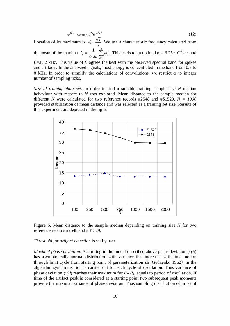
10

ϕ (k) = const ⋅ω 2ke−α 2ω 2 (12)

Location of its maximum is ωk* =

kα

. We use a characteristic frequency calculated from

the mean of the maxima ∑=⋅

=3

1

*

231

kkcf ω

π. This leads to an optimal α = 6.25*10-5 sec and

fc=3.52 kHz. This value of fc agrees the best with the observed spectral band for spikes and artifacts. In the analyzed signals, most energy is concentrated in the band from 0.5 to 8 kHz. In order to simplify the calculations of convolutions, we restrict α to integer number of sampling ticks. Size of training data set. In order to find a suitable training sample size N median behaviour with respect to N was explored. Mean distance to the sample median for different N were calculated for two reference records #2548 and #S1529. N = 1000 provided stabilisation of mean distance and was selected as a training set size. Results of this experiment are depicted in the fig 6.

0

5

10

15

20

25

30

35

40

100 250 500 750 1000 1500 2000N

Dm

ean

S15292548

Figure 6. Mean distance to the sample median depending on training size N for two reference records #2548 and #S1529. Threshold for artifact detection is set by user. Maximal phase deviation. According to the model described above phase deviation γ (θ) has asymptotically normal distribution with variance that increases with time motion through limit cycle from starting point of parameterization θ0 (Gudzenko 1962). In the algorithm synchronisation is carried out for each cycle of oscillation. Thus variance of phase deviation γ (θ) reaches their maximum for θ - θ0 equals to period of oscillation. If time of the artifact peak is considered as a starting point two subsequent peak moments provide the maximal variance of phase deviation. Thus sampling distribution of times of

11

the artifact maximal peak were used to estimate maximal phase deviation τmax . The difference between two subsequent peak moments equals

Δt p (k) = T + γ k (θ p ) − γ k−1(θ p ) (13) where θp is the phase of peak and γ k (θp ) is the phase deviation for the k-th artifact. Taking into account the short correlation time of the perturbation function, we considered γ k (θp ) as independent random variables with a variance σ p

2 = σ 2 (θ p ) . In this case it holds σ 2 (Δt p ) = 2σ p

2 . We estimated σ (Δt p ) directly from a set of peak times. Then the maximal phase deviation was fixed as τmax = 3σp. In the case of asymptotically normally distributed γ k (θp ), it corresponds to the confidence level 0.997. For example, for the signal #S1529 we obtained σp=2.5927⋅10-5 sec. The maximal phase deviation was fixed as τmax = 3σp = 7.7782⋅10-5 sec. Then τmax was adjusted by rounding to the nearest integer number of sampling ticks (4 ticks in case of sampling rate 48KHz). Basic radius R. The radius parameter is calculated according to the variance of the observed cycles of artifact. Namely the sampling fractiles are used. As we have mentioned above, the cycles x(θ), 0<θ ≤ T could be considered as normally distributed in the Euclidian space nTℜ . The difference of two independent x and y is also Gaussian. Thus the random values 2 x − Ex( ) and z = x-y are identically distributed as well as the Euclidian distances d 2 (x,Ex) = x - Ex 2 and d 2 (x,y) 2 = z 2 2. While the expectation of cycles is not known, we estimate the distribution density function of d 2 (x,y) 2 . For this purpose, we generated random pairs of cycles from the training set and we built a histogram. The position of a maximum was taken as a basic radius R, that corresponds approximately to the fractiles q0.34 – q0.35 . To calculate the fractiles, we approximate the histograms by χd

2 distributions. The effective degrees of freedom d were estimated as 7-8, which leads to the fractiles mentioned above. So 34.1 – 35.4% of cycles have to fall in the R-ball of limit cycle. In our experiments, we obtained 35-40% of cycles in the ball of radius R by direct count. 3. Experimental Results 3.1 Data Description Real Data Description. Eight records collected from five human patients during DBS surgery were used to test the algorithm. Neuronal activity is recorded before, during, and after high-frequency stimulation within the subthalamic nucleus, Globus Pallidus or Substantia Nigra (for some records the post-stimulation segment is not available). Signals were obtained using Medtronic external stimulator, and captured using AlphaOmega recording system. They were measured in volts after amplification. The records with a sampling rate of 48 kHz have 9 to 100 seconds duration, stimulation lasting 7-80 seconds. Periodic stimuli were delivered through microelectrodes placed 2mm apart in the same brain nucleus, with a frequency at 130Hz (i.e. with period approx 370 sampling ticks) and pulse duration 60 μs. Pulse intensities were in the range of 1000 µA - 6000 µA. Synthetic Dataset. In order to explore algorithm’s behaviour depending on artifact amplitude we constructed a set of artificial signals with predefined ASR. To the record (6-second segment) containing artifacts with no neuronal activity another signal with

12

single-neuron spikes and no stimulation were added. Appropriate constant K gives desired value of ASR:

XSyntethic (t) = XArtifacts(t) +K XSingle-Neuron(t). Collection of such signals for ASR from 2 to 20 was generated. 3.2 Tests of the Algorithm To compare the quality of signal description by the standard model with additive noise (Eq.1) and model (Eq.2) the appropriate phase dependent standard deviations (Fig. 4) of the residuals STD(t), 0 < t ≤ T were calculated. We estimated standard deviationsσξ (t) , 0 < t ≤ T of additive noise ξk (t) in the model (Eq.1) and σ n1

(θ ) , 0 < θ ≤ T, standard deviations of n1(t), the first coordinates of the vectors of normal deviation (Eq.5). Values n1(t) represent the residuals of artifacts in the time domain for the model (Eq.2). Eight real data records described above were used to estimate STD(t). The phase model (Eq.2) produces much smaller variances especially close to the peak (Table 1). The sums of STD across residual were in average 2.13 times less and the maxima of STD were 1.5-2.1 (1.8 in average) times less for the phase model. Table 1: STD of artifact residuals in the artifact peak zone

Filtering in time domain Filtering in phase space Record # Max. STD Sum of STDa

across residual Max. STD Sum of STDa

across residual 2548 0.106611 4.34 0.057173 1.76

S1529 0.118543 2.57 0.058254 1.251 F096K 0.088063 6.22 0.018505 2.04 N0047 0.151444 3.52 0.095315 1.84 N0023 0.14377 3.96 0.072804 2.20

DUG1581 0.086437 3.86 0.051635 1.935 DUG4821 0.201742 3.88 0.147963 2.18

S467 0.037689 1.646 0.023234 0.822 Tests of the Algorithm with Synthetic data. The test intends to reveal what happens to spike trains and spikes itself in presence of stimuli and cleaning procedures. Spike trains obtained from an original signal of neuronal activity XSingle-Neuron(t) before mixing with artifacts and after full processing were compared. Simple threshold filter was used for spike trains extraction. Percentages of spikes found in processed signal at their correct positions were measured. Let us note that summation of signals with coefficient K changes the spike-noise ratio. The graphs of errors of spike detection depending on ASR and corresponding SNR are depicted in the Fig. 7a, 7c. Fig. 7b represents variances of two first principal components of spikes depending on ASR. We can see that spikes rest practically intact up to ASR about 10-12.

13

a)

Wrong Spike Detection

0

2

4

6

8

0 2 4 8 12 16ASR

Erro

r %

b) PC Standard Deviation

0

0.25

0.5

0.75

1

1.25

1.5

0 2 4 8 12 16ASR

STD

PC1PC2

c) SNR vs ASR before processing

0

0.5

1

1.5

2

2.5

3

3.5

4

0 2 4 8 12 16ASR

SNR

Figure 7. Post-filtering spike quality for synthetic data: a) percentage of errors of spike detection after filtering; b) variance of first two principal components for detected spikes; (c) SNR in synthetic signals used for the test. ASR=0 corresponds to original neuron activity with no stimulation added. 3.3 Real Data filtering The records described above were used to test the algorithm on real data. The signals are characterized by ASR ∈ [1.3, 14], ANR ∈ [3, 160] and SNR ∈ [1.4, 5.1]. Examples of original and filtered signals are shown in Fig. 1,2. Fig. 3 display signal sliced into sets of stimulation-period windows, before and after filtering. The figure demonstrates the shape of the original artifacts and of the residuals left after full processing. One can see also the neuronal spikes. Phase portraits in 3D of appropriate artifact sets are depicted in the Fig. 8. In the Fig 8a we can see spike trajectories (smaller orbit) of record #2548. a)

14

b)

-0.100.10.20.3

-0.050

0.050.1

-0.04

-0.02

0

0.02

0.04

x1x2

x3

-0.10

0.10.2

0.3

-0.050

0.050.1

-0.04

-0.02

0

0.02

0.04

x1x2

x3

Figure 8. Artifact trajectories in the phase space projection with coordinates D1x(t), D2x(t), D3x(t) for records #2548 (a) and #S1529 (b). Dependences between Artifact Spike Ratio before and after signals filtering, both in phase space and time domain are presented in the Fig 9. For comparison, we have also shown such results for synthetic data. As a result we can see curves being in good fit with real-data cases.

15

0

0.5

1

1.5

2

2.5

0 2 4 6 8 10 12 14 16 18 20 22 24

ASR Original

ASR

Pro

cess

edPhase Space SyntheticTime Domain SyntheticPhase SpaceTime Domain

Figure 9. Residual-spike ratio depending on pre-filtering ASR comparing time-domain and phase-space algorithms for synthetic and real data. Results for eight real records (markers) and synthetic signals (dash and continuous lines) are in a good fit. 4. Discussion The most commonly known algorithm for artifact subtraction (Hashimoto et al, 2002) is based on making artifact templates by averaging the set of peri-stimulus segments in time domain. After template subtraction 11% (DBS 130Hz) of record time are removed from the signal. This paper presents a new method for the filtering of the signal of neuronal activity during DBS with artifact template subtraction. It is based on nonlinear oscillation model with perturbation as a basic model of stimulus artifacts instead of model with additive noise. This model explains signal distortion in both amplitude and phase. The set of synchronised in phase space artifact is used to estimate 3D artifact template with mean or median. Template is subtracted from the signal according to synchronization. The use of the proposed method and algorithms allows a 2-3 times reduction of the residual artifact of stimulation in comparison with the standard model with additive noise. The tests with artificial signals that are the combination of real signals of neuronal activity and stimulus artifacts showed that spike trains are less corrupted. This promising approach will enable analysis of neuronal activity during DBS to more effectively study the mechanism and to therefore improve the DBS technique. Let us note that all data in this paper were obtained using standard elecrophysiological equipment. Such devices limit suitable artifact amplitude because of their insufficient dynamic range. In future research, the use of dedicated (more precise) recording systems will allow studding the problem of filtering of stimulus artifacts of higher amplitude and variance. Acknowledgment

16

This study was partially supported by a Medtronic Grant to INSERM U318. The authors wish to express their appreciation to Dr. Brigitte Piallat for providing the recording used in the studies. References 1. Benabid A.L., Wallace B., Mitrofanis J., Xia R., Piallat B., Chabardes S., Berger F., A putative generalized model of the effects and mechanism of action of High Frequency Electrical Stimulation of the Central Nervous System, Acta neurol. Belg., 2005, 105 :149-157.

2. McIntyre C.C., Grill W.M., Sherman D.L., Thakor N.V., Cellular effects of deep brain stimulation: model-based analysis of activation and inhibition, J.Neurophysiol. 2004, 91:1457-1469.

3. Roby RJ, Lettich E. A simplified circuit for stimulus artefact suppression. Electroenceph. Clin. Neurophys. 1975;39:85–7.

4. Knaflitz M, Merletti R. Suppression of stimulus artifacts from myoelectric-evoked potential recordings. IEEE Trans Biomed Eng, 1988; 35(9):758–63.

5. Solomonow M, Baratta R, Miwa T, Shoji H, D’Ambrosia R. A technique for recording the EMG of electrically stimulated skeletal muscle. J. Orthoped., 1985;8(4):492–5.

6. Roskar E, Roskar A. Microcomputer based electromyographic recording system with stimulus artefact suppression. In: Third Medical Conference on Biomedical Engineering, 1983. Yugoslavia, Portoroz.

7. Rossi L, Foffani G, Marceglia S, Bracchi F, Barbieri S, Priori A. An electronic device for artefact suppression in human local field potential recordings during deep brain stimulation. J Neural Eng. 2007 Jun;4(2):96-106. Epub 2007 Mar 13.

8. Blogg T, Reid WD. A digital technique for stimulus artifact reduction. Electroencephalogr. Clin. Neurophysiol. 1990;76:557-61

9. Winchman T. A digital averaging method for the removal of stimulus artifacts in neurophysiologic experiments. J. Neurosci. Meth, 2000 ;98:57–62.

10. Wagenaar D.A.,. Potter - S.M. Real-time multi-channel stimulus artifact suppression by local curve fitting - DA J. Neurosci. Methods, 2002

11. Derek T. O’Keeffe, Gerard M. Lyons, Alan E. Donnelly, Ciaran A. Byrne. Stimulus artifact removal using a software-based two-stage peak detection algorithm. Journal of Neuroscience Methods; 109, 2001, 137–145

12. Hines AE, Crago PE, Chapman GJ, Billian C. Stimulus artifact removal in EMG from muscles adjacent to stimulated muscles. J. Neurosci. Meth., 1996; 64:55–62.

13. Hashimoto T, Elder C.M., Okun M.S., Patrick S.K., Vitek J.L., Stimulation of the subthalamic nucleus changes the firing pattern of pallidal neurons, J.Neurosci., 2003, 23 :1916-1923.

14. Hashimoto T, Elder CM, Vitek JL. A template subtraction method for stimulus artifact removal in high-frequency deep brain stimulation. J Neurosci Methods, 2002, 113:181-186.

17

15. Tai CH, Boraud T, Bezard E, Bioulac B, Gross C, Benazzouz A. Electrophysiological and metabolic evidence that high-frequency stimulation of the subthalamic nucleus bridles neuronal activity in the subthalamic nucleus and the substantia nigra reticulata. FASEB J. 2003 Oct;17(13):1820-30

16. Gudzenko, L.I., Statistical method for self-oscillating system characteristics detection, Izvestiia Vuzov Radiophysics, 1962, 5: 573-587.

17. Aksenova, T.I.; Chibirova O.K., Dryga, O.A., Tetko, I.V.; Benabid A.-L.; Villa,A.E.P.; An unsupervised automatic method for sorting neuronal spike waveforms in awake and freely moving animals. Methods, 2003, 30: 178-187.

Chapter 5

Sensors and Actuators B xxx (2004) xxx–xxx

Preprocessing of matrix QCM sensors data for theclassification by means of neural network

A.M. Reznik∗, A.A. Galinskaya, O.K. Dekhtyarenko, D.W. NowickiThe Institute of the Mathematical Machines and Systems, National Academy of Sciences of Ukraine, 42 Glushkov Ave, Kiev 03187, Ukraine

Abstract

An experimental comparison of linear and non-linear pre-processing methods for olfactory data is made. The original data are formedby 280 values of reaction from six quartz crystal microbalance (QCM) sensors taken at 1 s intervals. Data vectors are processed with thenon-linear maximum filter or by the linear averaging filter and are used as inputs of a feedforward neural network using the back-propagationlearning rule, one hidden layer containing from 5 to 15 neurons. The filter window size is 5–10.

The learning set is composed of 60 sensor reactions for six types of cologne. The neural network correctly classifies 82–86% ofindependent examples. The usage of the maximum filter with a small window size allows an increase of the classification rate by 3–5%.The best results (86%) are obtained when only first 50 measurements of sensor reaction are used.© 2004 Elsevier B.V. All rights reserved.

Keywords: Neural networks; Odour recognition; QCM sensors; Data preprocessing

1. Introduction

The usage of neural networks for the odour recognition isbased on their ability to identify the differences in responseto the sensors reacting in different ways for various aromasubstances[1,2]. The values of matrix sensor reactions ana-lyzed by the neural network contain redundant componentsand fluctuations that complicate the learning process anddistort classification results. In order to depress these fac-tors data preprocessing is used which includes filtration andnormalization to the [−1, +1] range, corresponding to theneuron activation values. In a number of cases the effective-ness of a neural network could be increased with the helpof the non-linear transform of input data. This phenomenonis caused by the change of Vapnik–Chervonenkis dimen-sion and is used in SVM classifier[3], which resolves themost difficult classification problems where the data are notlinearly separable. The same principle of non-linear prepro-cessing operations can be used to improve the classificationof linearly inseparable data by a feedforward neural network.

At the present time there are two dominant methods ofapproach to the preprocessing of olfactory data classified bya neural network.

∗ Corresponding author. Tel.:+340 44 2665548; fax:+340 44 2666457.E-mail address: neuro@immsp.kiev.ua (A.M. Reznik).

1. The training of a neural network with redundant archi-tecture followed by the removal of elements of little in-formation (connections and/or neurons).

2. The usage of the principle components technique to re-duce the data redundancy at the input of a network.

In the first case, the preprocessing functions are laid on theneurons of the first hidden layer and their required functionsare formed during the training process. The training of aneural net consists of a few phases. At the end of each phasethe information density, i.e. the influence of each component(connection/neuron) on a behaviour of the entire network isestimated and the least significant components are removed.This method, also known as “pruning”[4], is effective incases when the network learning process has a sufficientdegree of convergence. Unfortunately, it is not always easyto find such a network.

The method of principal components (often referred asprincipal components analysis (PCA)) is based on an extrac-tion of senior components of data decomposition into thebasis formed by the correlation matrix eigenvectors. Thesesenior components hold the most signal energy and the ratioof their amplitudes is often sufficient to identify the sensorreaction[5]. Usually, the method is used to increase infor-mation density and to decrease the dimension of input datafed to a neural network[6].

The PCA method exploits the model of Gaussian distri-bution of data. The experimental comparison[7] of the op-

0925-4005/$ – see front matter © 2004 Elsevier B.V. All rights reserved.doi:10.1016/j.snb.2004.05.047

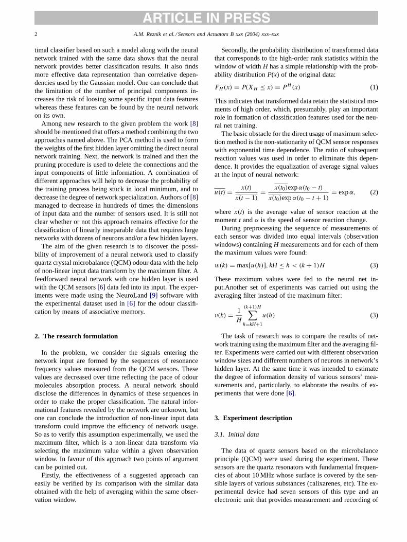
2 A.M. Reznik et al. / Sensors and Actuators B xxx (2004) xxx–xxx

timal classifier based on such a model along with the neuralnetwork trained with the same data shows that the neuralnetwork provides better classification results. It also findsmore effective data representation than correlative depen-dencies used by the Gaussian model. One can conclude thatthe limitation of the number of principal components in-creases the risk of loosing some specific input data featureswhereas these features can be found by the neural networkon its own.

Among new research to the given problem the work[8]should be mentioned that offers a method combining the twoapproaches named above. The PCA method is used to formthe weights of the first hidden layer omitting the direct neuralnetwork training. Next, the network is trained and then thepruning procedure is used to delete the connections and theinput components of little information. A combination ofdifferent approaches will help to decrease the probability ofthe training process being stuck in local minimum, and todecrease the degree of network specialization. Authors of[8]managed to decrease in hundreds of times the dimensionsof input data and the number of sensors used. It is still notclear whether or not this approach remains effective for theclassification of linearly inseparable data that requires largenetworks with dozens of neurons and/or a few hidden layers.

The aim of the given research is to discover the possi-bility of improvement of a neural network used to classifyquartz crystal microbalance (QCM) odour data with the helpof non-linear input data transform by the maximum filter. Afeedforward neural network with one hidden layer is usedwith the QCM sensors[6] data fed into its input. The exper-iments were made using the NeuroLand[9] software withthe experimental dataset used in[6] for the odour classifi-cation by means of associative memory.

2. The research formulation

In the problem, we consider the signals entering thenetwork input are formed by the sequences of resonancefrequency values measured from the QCM sensors. Thesevalues are decreased over time reflecting the pace of odourmolecules absorption process. A neural network shoulddisclose the differences in dynamics of these sequences inorder to make the proper classification. The natural infor-mational features revealed by the network are unknown, butone can conclude the introduction of non-linear input datatransform could improve the efficiency of network usage.So as to verify this assumption experimentally, we used themaximum filter, which is a non-linear data transform viaselecting the maximum value within a given observationwindow. In favour of this approach two points of argumentcan be pointed out.

Firstly, the effectiveness of a suggested approach caneasily be verified by its comparison with the similar dataobtained with the help of averaging within the same obser-vation window.

Secondly, the probability distribution of transformed datathat corresponds to the high-order rank statistics within thewindow of widthH has a simple relationship with the prob-ability distributionP(x) of the original data:

FH(x) = P(XH ≤ x) = PH(x) (1)

This indicates that transformed data retain the statistical mo-ments of high order, which, presumably, play an importantrole in formation of classification features used for the neu-ral net training.

The basic obstacle for the direct usage of maximum selec-tion method is the non-stationarity of QCM sensor responseswith exponential time dependence. The ratio of subsequentreaction values was used in order to eliminate this depen-dence. It provides the equalization of average signal valuesat the input of neural network:

u(t) = x(t)

x(t − 1)= x(t0)expα(t0 − t)

x(t0)expα(t0 − t + 1)= expα, (2)

where x(t) is the average value of sensor reaction at themomentt andα is the speed of sensor reaction change.

During preprocessing the sequence of measurements ofeach sensor was divided into equal intervals (observationwindows) containingH measurements and for each of themthe maximum values were found:

w(k) = max[u(h)], kH ≤ h < (k + 1)H (3)

These maximum values were fed to the neural net in-put.Another set of experiments was carried out using theaveraging filter instead of the maximum filter:

v(k) = 1

H

(k+1)H∑

h=kH+1

u(h) (3)

The task of research was to compare the results of net-work training using the maximum filter and the averaging fil-ter. Experiments were carried out with different observationwindow sizes and different numbers of neurons in network’shidden layer. At the same time it was intended to estimatethe degree of information density of various sensors’ mea-surements and, particularly, to elaborate the results of ex-periments that were done[6].

3. Experiment description

3.1. Initial data

The data of quartz sensors based on the microbalanceprinciple (QCM) were used during the experiment. Thesesensors are the quartz resonators with fundamental frequen-cies of about 10 MHz whose surface is covered by the sen-sible layers of various substances (calixarenes, etc). The ex-perimental device had seven sensors of this type and anelectronic unit that provides measurement and recording of

A.M. Reznik et al. / Sensors and Actuators B xxx (2004) xxx–xxx 3

-1200

-1000

-800

-600

-400

-200

00 50 100 150 200 250

time

freq

uen

cy s

hif

t

Fig. 1. Sensors’ response for the ethanol sample.

sensors’ fundamental frequencies with 1 s interval for theduration of 280 s. The result of each experiment is the se-quence of 1960 integer measurement values.Fig. 1 depictsan example of such a sequence obtained for the ethanol sam-ple.

The list of substances used and their total amount is shownin Table 1.

3.2. Neural network

Neural network of feedforward type contained one hid-den layer with 5, 10 or 15 neurons. Data coming to each ofthe net inputs were normalized to the [0, 1] range. Normal-izing coefficients were calculated using the training dataset.The neural network was trained using the standard onlineback-propagation algorithm. The learning rate was set to0.05 and the moment coefficient was 0.15. Save Best Methodwas used during the training that lasted for 5000 epochs.Output neurons were used in classification mode, i.e. thenetwork reaction was determined according to the maximumvalue of the post-synaptic potential. Experiments were car-ried out using the NeuroLand software package[9].

Taking into account a comparably small amount of inputdata, we used six variants of decomposition of initial datasetinto train and independent test parts. These datasets wereformed by random selection of 20 train examples from theinitial data. Every variant of selection contained examplesof all analyzed classes. Thus, for each reported classificationresult network training and testing was made six times with

Table 1Classes of chemical images

Class Substance Number of images

1 Ethanol 112 Landish 53 Russki Les 84 Roksolana 65 Shipr 126 Siren 157 Water 3

independent parts of data and final result was derived as theaverage of these tests.

4. Experimental results

The results of testing of the neural network with differentnumber of hidden neurons are depicted inFigs. 2–4. Theaverage percentage values of correctly classified odour pat-terns are shown for the maximum filter and the averaging fil-ter depending on the observation window size. These resultswere obtained using three subsets of sensor reaction values:values collected during the first 50 s, collected in the interval50–200 s, and all 280 values of reaction of each sensor.

Comparing the results obtained, one may note that asthe sizes of hidden layer and observation window increases,the difference between two types of preprocessing vanishes.The greatest difference is observed with the window sizeof 3. The network with five hidden neurons plus using thefirst 50 values of sensor reaction had the highest results.The maximum classification value, about 86% of correctresponses, was obtained using the maximum filter with thewindow size of 3. Under the same conditions the resultsof averaging filter were 6% lower. Networks with greaternumber of hidden neurons also exhibited better results withthe maximum filter (about 83.5%).

The results of experiments estimating the influence ofused normalization methods on the classification results aregiven onFigs. 5 and 6. These figures depict the dependen-cies of correct classification value on the number of hiddenneurons for the original data and the data normalized us-ing (1). The experiments were made with the complete datavectors containing 280 values and with truncated ones thatcontain reaction values collected for the first 50 s. The re-sults for the maximum filter are shown onFig. 5 and theresults for the averaging filter are shown onFig. 6. In bothexperiments the observation window size was set to 3.

For the normalized input data the best results—about 86%are obtained using the maximum filter with the network hav-ing five hidden neurons and truncated data vectors. With-out normalization both the maximum and averaging filters

4 A.M. Reznik et al. / Sensors and Actuators B xxx (2004) xxx–xxx

Fig. 2. Classification results for the network with five hidden neurons and normalized input data.

Fig. 3. Classification results for the network with 10 hidden neurons and normalized input data.

Fig. 4. Classification results for the network with 15 hidden neurons and normalized input data.

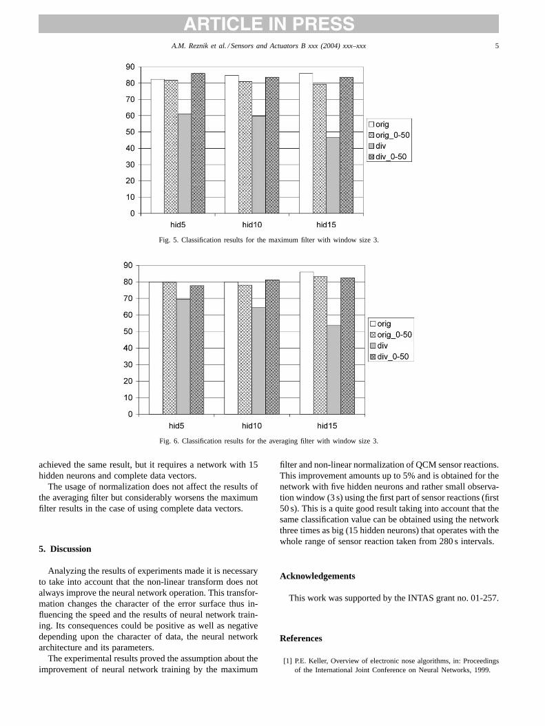
A.M. Reznik et al. / Sensors and Actuators B xxx (2004) xxx–xxx 5

Fig. 5. Classification results for the maximum filter with window size 3.

Fig. 6. Classification results for the averaging filter with window size 3.

achieved the same result, but it requires a network with 15hidden neurons and complete data vectors.

The usage of normalization does not affect the results ofthe averaging filter but considerably worsens the maximumfilter results in the case of using complete data vectors.

5. Discussion

Analyzing the results of experiments made it is necessaryto take into account that the non-linear transform does notalways improve the neural network operation. This transfor-mation changes the character of the error surface thus in-fluencing the speed and the results of neural network train-ing. Its consequences could be positive as well as negativedepending upon the character of data, the neural networkarchitecture and its parameters.

The experimental results proved the assumption about theimprovement of neural network training by the maximum

filter and non-linear normalization of QCM sensor reactions.This improvement amounts up to 5% and is obtained for thenetwork with five hidden neurons and rather small observa-tion window (3 s) using the first part of sensor reactions (first50 s). This is a quite good result taking into account that thesame classification value can be obtained using the networkthree times as big (15 hidden neurons) that operates with thewhole range of sensor reaction taken from 280 s intervals.

Acknowledgements

This work was supported by the INTAS grant no. 01-257.

References

[1] P.E. Keller, Overview of electronic nose algorithms, in: Proceedingsof the International Joint Conference on Neural Networks, 1999.

6 A.M. Reznik et al. / Sensors and Actuators B xxx (2004) xxx–xxx

[2] J.W. Gardner, P.N. Bartlett. Electronic Noses, Principles and Appli-cations, Oxford University Press, Oxford, 1999.

[3] V. Vapnik, Statistical Learning Theory, Wiley, 1998, pp. 736.[4] S. Haykin, Neural Networks: A Comprehensive Foundation, second

ed., Prentice Hall Inc., 1999, pp. 842.[5] I.V. Kruglenko, B.A. Snopok, Y.M. Shirshov, E.F. Venger, Digital

aroma technology for chemical sensing: temporal chemical images ofcomplex mixtures, Semicond. Phys., Quant. Electron. Optoelectron.3 (4) (2000) 529–541.

[6] A.M. Reznik, Yu. M. Shirshov, B.A. Snopok, D.W. Nowicki, A.K.Dekhtyarenko, I.V. Kruglenko, Associative memories for chemicalsensing, in: Proceedings of the International Conference on NeuralInformation Processing, Singapore, 2002.

[7] A.M. Reznik, A.A. Galinskaya, K.M. Kuzhel, On the informationdensity of Gaussian components used for the classification of ultra-sonic location signals, in: Proceedings of the Eighth All-Russian Con-ference on Neurocomputers and Their Applications, 21–22 March2002, Moscow, Russia, pp. 244–250.

[8] Z. Boger, R. Cavicchi, S. Semancik, Analysis of conductometricmicrosensor responses in 36-sensor array by artificial neural net-works modeling, in: Proceedings of the International Symposium onISOEN’02, Rome, 2002.

[9] A.M. Reznik, E.A. Kalina, A.S. Sitchov, E.G. Sadovaya, O.K.Dekhtyarenko, A.A. Galinskaya, multifunctional neurocomputer Neu-roLand, in: Proceedings of the International Conference on InductiveSimulation, vol. 1 (4), Lviv, Ukraine, 2002, pp. 82–88.

Biographies

A.M. Reznik, Head of Department of Neural Technologies in Instituteof Mathematical Machines and Systems, received degree in technicalsciences in 1998, PhD in technical sciences in 1968 and MS in Kiev

Polytechnic Institute, Electro-Acoustical Department in 1958. The fieldsof interest are object recognition, acoustics and neural networks.

A.A. Galinskaya, Researcher, Institute of Mathematical Machines and Sys-tems. She is a post-graduate student in Institute of Mathematical Machinesand Systems, NAS Ukraine since 2002, received MS in informatics, Na-tional Technical University of Ukraine “Kiev Politechnical Institute” in2002 and BS in applied mathematics, National Technical University ofUkraine “Kiev Politechnical Institute” in 2000. The fields of interest areartificial neural networks, system programming, mathematical modeling,data processing and pattern recognition.

O.K. Dekhtyarenko, Researcher, Institute of Mathematical Machines andSystems. He is a post-graduate student at Educational and ScientificCenter of Physics and Technology, National Academy of Science ofUkraine. He received his MS in applied informatics at National TechnicalUniversity of Ukraine “Kiev Polytechnic Institute”, Department of Physicsand Technology in 2002 and a Bachelor’s degree in applied mathematicsin 2000. The fields of interest are neural networks, data processing,object-oriented analysis, programming and design.

D.W. Nowicki, Researcher, Institute of Mathematical Machines and Sys-tems. He is a PhD student at Universite Paul Sabatier Toulouse, France.PhD degree in applied mathematics expected in 2005. Also, is a PhDstudent at Moscow Institute of Physics and Technology (Kiev Subdivi-sion), PhD degree in theoretical computer science expected in 2003. MSin applied mathematics was received at Moscow Institute of Physics andTechnology in 2000 BS in applied mathematics and physics, MoscowInstitute of Physics and Technology in 1999. The fields of interest areneural networks, artificial intelligence, mathematical programming, datamining, time series analysis, natural language processing, non-linear dy-namics, graph theory, theoretical computer science, routing algorithms,stochastic processes, simulation techniques, etc.

ASSOCIATIVE MEMORIES FOR CHEMICAL SENSING

Reznik A.M.1, Shirshov Yu. M.2, Snopok B.A.2, Nowicki D.W.1, Dekhtyarenko A.K.1, Kruglenko I. V.2

1Institute of Mathematical Machines and Systems of NAS of Ukraine

2Institute of Semiconductor Physics of NAS of Ukraine neuro@immsp.kiev.ua

ABSTRACT

We consider application of neural associative memories to chemical image recognition. Chemical image recognition is identification of substance using chemical sensors’ data. The primary advantage of associative memories as compared with feed-forward neural networks is high-speed learning. We have made experiments on odour recognition using hetero-associative and modular auto-associative memories. We have also tested backpropagation NNs with one hidden layer. Associative memories displayed recognition quality not worse than backpropagation networks.

1.INTRODUCTION

Chemical image (CI) recognition is identification of substance using chemical sensors’ data. To solve these problems one generally use classical methods of statistical analysis such as principal component (PCA), discriminant factor analysis et c. Nowadays Feed-Forward neural networks and Kohonen’s self-organizing maps are also introduced (applied)[1,2]. In this case one can reduce system tuning to training neural networks using experimental data. Unfortunately, training neural networks takes a lot of time, so their application is often discouraged. Therefore, associative memories are welcomed because of their greatly faster training (only within one iteration for Hopfield-type networks) [3]. The major disadvantage of associative memories is a rather low generalizing ability that increases sensor stability requirements. Although, new learning algorithms and architectures of associative memory enable to overcome these difficulties. In particular, modular and hetero-associative memories could be used.

In the case of piezoelectric transducers adsorption process can be directly characterized with the resonance frequency change values (at different moments) and their time derivatives, as well as various combinations of the above values. One should specially note that use of

approaches based on experimental curves fitting with analytical functions to obtain the response parameters seems to be inappropriate in this case. The reason is that very often the simple kinetic models for adsorption cannot adequately describe the curves for the sensor array response, because of Multi-Component Mixture’s (MCM) components diffusion into the sensitive coating bulk, change of its structure, uncontrolled fluctuation of temperature and pressure. Indeed, if one uses for MCM CI formation only stationary values (i.e., those that characterize a system after an equilibrium has established), then one may omit important information concerning character of interaction between highly volatile components with different mobilities/activities and the sensitive layer. And the sensitive layer prehistory strongly affects the features of the receptor/analyte interaction in the initial portion of the kinetic curve. Thus the problem how to choose an optimal range of the initial data that could take into account the kinetic and stationary features of the sensor array response, as well as some leveling effects of the pre-starting procedure, are important for both fundamental science and practical applications.

The goal of this paper is to prove possibility of practical application of associative memories to chemical image recognition. We have made a series of experiments on learning to recognize some different substances (perfumes, ethanol, et c.) using associative and Feed-Forward neural networks. The research was done using neural software package NeuroLand designed at Institute of Mathematical Machines and Systems of NASU and the multi-sensor piezo-crystal gas analyzer designed at Institute of Semiconductor Physics of NASU [3].

2.EXPERIMENTAL TECHNIQUE

AND GIVEN DATA To obtain chemical images we have used an experimental assembly based on Quartz Crystal Microbalance (QCM). The universal neural computer NeuroLand was used to process digitised data: It enables to model different types of neural networks, train and test them.

Fig. 1. Overall view of QCM experimental appliance

2.1.The QCM experimental assembly

In sensors based on piezoelectric physical transducers there is the dependence between resonance frequency f of acoustical resonator and mass Δm of a substance at sensor’s surface. It is used to detect intermolecular interactions. For measurements in gas phase dependence between the resonance frequency change Δf and the mass change Δm on its surface is assumed to be linear in accordance with well-known Sauerbreu’s equation.

In this work QCM-based arrays were used as prototypes an artificial nose for testing of some perfumes and vapors. For experiments a full-automatic 10-MHz quartz crystals (AT-cut, RK169) based on 8-channel systems with a measurement step of 1 s were used. The e-Nose instrument involves the following units: a thermostatic measuring chamber with a flow-type sensor array; a quartz oscillator unit; a frequency counter with RS232 interface based on AT89C2051 microprocessor; a gas mixtures generator; a computerized system to collect and process information. The general view of the e-Nose instrument is shown in Fig. 1. The sensor units have a specially designed Teflon holder in which the quartz crystals were fixed along its perimeter. So, only one side of quartz crystal was covered by sensing material and contacted with changing ambient. The flow of buffer gas (argon) was used for recovery thin film coating after adsorption phase. It was shown that construction with fixation of quartz crystals along perimeter is preferable due to strong decrease of noise.

The measuring procedure involved the following stages at the temperature 37±0.3 ОС: argon circulation until the transducer frequency is stabilized (±2 Hz); vapor-gas mixture circulation at a gas-carrier rate of 20-50 ml/min.; circulation with argon air until the QCM frequency returns to its initial value.

The following five types of perfumes (GOST 17237-93) as typical MCM were tested: éau-de-Cológne “Siren”,

“Landish” (produced by “Effect”, Kharkov); éau-de-Cológne “Russkij Les” (OAO, produced by “Kombinat Krimskaja Rosa”, Simferopol), éau-de-Cológne “Shipr” and “Roksolana” (produced by PKK “ROSO”, Zhovka) as well as water ant ethyl alcohol. The sample volume was 12 ml in every case.

Fig. 2. Response of 7 sensors (A, B, D-H)

for ethanol's smell

Table 1. Classes of chemical images

Class # Substance Number of images 1. Ethanol 11 2. “Landish” 5 3. “Russki Les” 8 4. “Roksolana” 6 5. “Shipr” 12 6. “Siren” 15 7. Water 3

2.2Input data for training NN

For numerical experiments we have used measurements for seven substances (see Table 1).

Most of chemical images contained data for 7 sensors. Time series for each sensor were 286 ticks long. For instance, in the Fig. 2 we can see 7 sensors’ output for the odour of ethanol.

Approximately, these regularities are close to exponential. On the other hand, a noise component is rather strong, and starting pieces of time series are sometimes instable. Note that different chemical images for each class are also highly scattered. For certain images intra-class dispersion may exceed 10%.

Data might enter into NN’s input immediately, or after PCA preprocessing. Principal components were computed using the entire training sample. Otherwise NNs were trained and tested using 6 classes only (57 images, classes #1-6).

In this paper we evaluate maximum classification quality using different NNs. Also we try to find optimal

parameters of preprocessing technique. Sample window metrics (size and starting point) and number of PCs were such tuneable parameters.

The “correctly recognized images”/”all test images” ratio is called classification rate. Each value of classification rate was obtained in averaging over several “training/test” dissections of the sample. These dissections were randomly generated holding all other experiment conditions constant. To determine recognition quality we have used 50 for the modular associative classifier, and 10 dissections for the hetero-associative one. For the Feed-Forward NN recognition quality was estimated in averaging over 10 results with different initial states of the network.

3. ARCHITECTURE AND ALGORITHMS OF

NEURAL NETWORKS 3.1. Associative memories Associative memories are preferred due to fast

learning done within single iteration in computing all neurons’ weights. Unfortunately, most common models like Hopfield networks or bi-directional associative memories deal with bipolar data only [4]. It’s needed to use convergence examination for restoration of corrupted data. But we need only classify chemical sensors’ data. So, we should build an associative-memory classifier, which will use real data vectors. We have considered two associative memory classifiers: hetero-associative and a modular one.

3.1.1.Hetero-assaciative classifier

Hetero-associative classifier is a single-layered network with linear activation function; chemical sensors’ data are directed to its N inputs. The quantity of neurons K is equal to number of classes (chemical substances). Weights are computed using pseudo-inverse learning rule [6]. These rules cold be obtained solving stability equation:

ii yBx = , (1) where: B is a K×N weight matrix of thee network, xi –

N-dimensional input vector, yi – K-dimensional output vector,its k-th component is equal to +1 if corresponding input belongs to class k, the rest of components are –1.

The training data array could be represented as two matrices: X contains M data vectors, and Y contains M desired network’s responses.

Solution of (1) is: += YXB , (2)

where X+ is a pseudo-inverse matrix to X. X+ is usually computed using Greville’s formulae [6]. 3.1.2. Modular auto-associative classifier

It consists of K neural modules; each of them is a conventional auto-associative network with real stored

images. Every module memorise N-dimensional data vectors for certain class. Data are memorised in k-th module computing projection matrix.

+= kkk XXC , (3) where Xk is a matrix containing data vectors for k-th

class. During recognition of an input vector z the post-

synaptic potential is computed: sk = Ck z, (4)

The letter is a projection of an input vector to linear span of training images for k-th class. The decision on belonging of input image is made maximizing scalar product:

qk = sk zT (5) where zT is a conjugate vector to z. The vector z is treated as belonging to k* that have

max* →kq . 3.2. Classifier using Feed-forward NN

Nowadays feed-forward neural networks and back-propagation learning algorithms are conventional techniques for chemical image recognition [1,2]. Strength and weaknesses of these NNs are well known; therefore we used such networks, basically, as a benchmark for associative-memory classifiers.

We have used NNs with one hidden layer. Hidden neurons had a sigmoid activation function, without a bias. Number of inputs is a dimension of input vector; for each class there is one output neuron. Data were normalized to [0, 1] range. We have tested networks with 5, 10 and 15 hidden neurons. Learning algorithm was a standard online backpropagation with learning rate 0.01 and momentum 0.15. Learning took 6000 epochs (about 10 min. of CPU time for Intel Celeron 600 MHz); so mean square error could be decreased to 10-2 - 5⋅10-3.

4.CLASSIFICATION QUALITY DEPENDING

ON SIZE OF TRAINING SAMPLE For these series of experiments we have used raw data

for all available ticks from 1st to 286th. In the case of usage of principal components the 50 highest ones were entered into classifier. Learning took about 4 sec. of CPU time for Intel Celeron 600 MHz. Results for modular and hetero-associative classifier are shown in Fig. 3.

Modular net

01020304050607080

0 1 2 3 4 5 6

Train Examples Count

Cla

ssifi

catio

n Pe

rcen

t

Normal

PCA

Fig. 3. Classification quality subject

to training image number .

Fig. 4. Recognition quality subject to initial measurement

and number of ticks used for modular network

For modular classifier the PC results are almost identical to ones for raw data. The best results – 70% – are achieved under use et least 4 learning examples. So, principal components are not strongly needed, because all useful information is extracted by NN itself.

For hetero-associative network classification quality decreases if training sample contains more than 60% of available vectors. It is caused by overflow of hetero-associative memory when number of memorized images exceeds 50% of data dimension. In this case data vectors consist of 50 components; there were 57 images, 60% of them (i.e. 34) were memorized. In a modular classifier

memorizes images of one class only; so there was no overflow

Fig. 5. Recognition quality subject to initial measurement and number of ticks used for hetero-associative network

5. DEPENDENCES ON WINDOW SIZE

These experiments were dedicated to find optimal parameters of data window for entering data into network. All types of NNs were tested. Modular network was trained using 4 examples for each class; training sample for hetero-associative one took 60% of available images. Positions of initial and final time ticks were scanned with step of 15 ticks.

Dependences of classification quality on size of data vector for associative memories are shown in the Fig. 4,5. Such dependences for Feed-forward NNs are displayed in Fig. 6. Starting point of a windows serves as a parameter in all the figures.

Note that both classifiers achieve best quality in excluding starting segment of data (100-150 ticks) and taking not more than 150-200 points for the network input. This may be explained taking into account instability of starting part of curves shown in fig 2. Note also that hetero-associative memory displays slightly better quality than modular one (73% vs. 71%). This might be caused only by experimental error.

Results for Feed-Forward networks show that initial parts of sensor response curves have low information. Best classification rates – 75-77% - were obtained excluding first 100 ticks and taking data for 50-100 ticks of the middle of response curves.

6. CLASSIFICATION RATIO SUBJECT TO

NUMBER OF PRINCIPAL COMPONENTS

These experiments were dedicated to find minimal quantity of PCs required to keep admissible classification rat for associative memories. Modular network was trained using 4 examples for each class; training sample for hetero-associative one took 60% of available images. Test results are shown in Fig. 7.

Fig. 6.Recognition quality subject to initial measurement and number of ticks used for feed forward networks with

different number of hidden neurons.

Fig. 7. Recognition quality subject to number of PCs for

hetero-associative and modular NNs

Modular network displays the best classification rate if more than 25 PCs are used; hetero-associative one requires 50 PCs. It is caused by overflow of hetero-associative memory when number of memorized images exceeds 50% of data dimension (cf. Fig. 3.). We can avoid memory overflow taking well over 34 components.

7. CONCLUSION

Experimental results described above show that associative memories provide approximately the same recognition quality as feed-forward neural networks. We stress that non-iterative nature of neural associative memories makes them quite attractive. This is not only high-speed learning but also learning independent on a (random) network initialization. Even a low generalisation ability of associative memories may be turned into advantage; using more stable chemical sensors they will be able to recognise thousands sorts of chemical substance.

8. ACKNOWLEDGEMENTS

This work was partially supported by INTAS grant No. 01POLL-0257.

Calyxarenes were kindly given to us by Prof. V.I. Kal’chenko (Institute of Organic Chemistry of NASU, Kyiv). Linear polyacenes were kindly given to us by Prof. Ya.I. Vertsimakha (Institute of Physics of NASU, Kyiv). Mycrocyclic compounds were kindly given to us by Prof. Ya.D. Lampeka (Institute of Physical Chemistry of NASU, Kyiv).

9.REFERENCES

1. Keller P. E. Overview of Electronic nose

Algorithms. Proc. Internat. Joint Conf. on Neural Networks, 1999

2. J.W. Gardner, P.N. Bartlett, Electronic Noses. Principles and Applications, Oxford University Press, 1999.

3. Reznik A.M "Non-Iterative Learning for Neural Networks" Proceedings International Joint Conference on Neural Networks, Washington DC, July 10-16, 1999

4. Kruglenko I.V., Snopok B.A., Shirshov Y.M., Venger E.F. Digital aroma technology for chemical sensing: temporal chemical images of complex mixtures // Semiconductor Physics, Quantum Electronics&Optoelectronics –2000-Vol.3-N4-P.529-541

5. Wasserman P.D., Neural computing. Theory and practice, ANZA Research Inc. VAN NOSTRAD REIHOLD, NY 1988

6. Kirichenko N. F, Reznik A.M, Schetenyuk S. P. “Matrix pseudo-inversion in the problem of design of associative memory”, Cybernetics and System Analysis, vol. 37 No. 3, pp. 308-316, 2001.