geoestadística en regiones heterogéneas con distancia ... · facultatdeciènciesmatemàtiques...
TRANSCRIPT
Facultat de Ciències MatemàtiquesDepartament d’Estadística i Investigació Operativa
Geoestadística en regiones heterogéneas condistancia basada en el coste
TESIS DOCTORALFacundo Martín Muñoz Viera
Director: Antonio López-QuílezFebrero 2013

Outline
Motivation: heterogeneous regions and covariance functions
Cost based-distance: a practical approach
Positive-definiteness violation
Positive-definiteness in Riemannian manifolds
Pseudo-Euclidean embedding
Alternative approaches
Conclusions and open lines of work
2 / 28
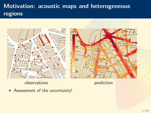
Motivation: acoustic maps and heterogeneousregions
observations predictionI Assessment of the uncertainty!
3 / 28
Covariance functions
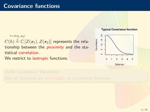
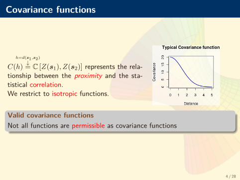
C(h)h=d(s1,s2)↓= C [Z(s1), Z(s2)] represents the rela-
tionship between the proximity and the sta-tistical correlation.We restrict to isotropic functions.
Valid covariance functionsNot all functions are permissible as covariance functions
4 / 28
Covariance functions
C(h)h=d(s1,s2)↓= C [Z(s1), Z(s2)] represents the rela-
tionship between the proximity and the sta-tistical correlation.We restrict to isotropic functions.
Valid covariance functionsNot all functions are permissible as covariance functions
4 / 28
Positive-definite functions
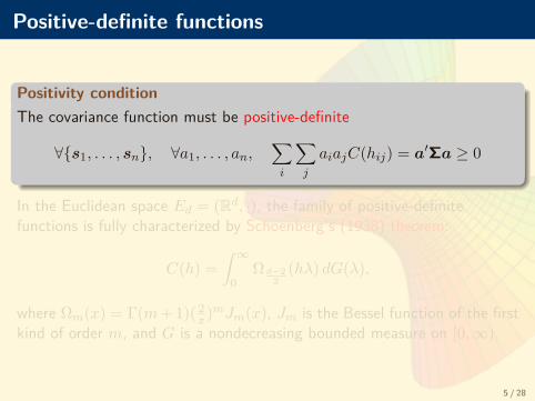
Positivity conditionThe covariance function must be positive-definite
∀s1, . . . , sn, ∀a1, . . . , an,∑i
∑j
aiajC(hij) = a′Σa ≥ 0
In the Euclidean space Ed = (Rd, ·), the family of positive-definitefunctions is fully characterized by Schoenberg’s (1938) theorem:
C(h) =∫ ∞
0Ω d−2
2(hλ) dG(λ),
where Ωm(x) = Γ(m+ 1)( 2x)mJm(x), Jm is the Bessel function of the first
kind of order m, and G is a nondecreasing bounded measure on [0,∞).
5 / 28

Positive-definite functions
Positivity conditionThe covariance function must be positive-definite
∀s1, . . . , sn, ∀a1, . . . , an,∑i
∑j
aiajC(hij) = a′Σa ≥ 0
In the Euclidean space Ed = (Rd, ·), the family of positive-definitefunctions is fully characterized by Schoenberg’s (1938) theorem:
C(h) =∫ ∞
0Ω d−2
2(hλ) dG(λ),
where Ωm(x) = Γ(m+ 1)( 2x)mJm(x), Jm is the Bessel function of the first
kind of order m, and G is a nondecreasing bounded measure on [0,∞).
5 / 28

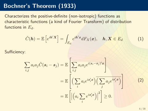
Bochner’s Theorem (1933)Characterizes the positive-definite (non-isotropic) functions ascharacteristic functions (a kind of Fourier Transform) of distributionfunctions in Ed.
C(h) = E[eih′X]
=∫Ed
eih′xdFX(x), h,X ∈ Ed (1)
Sufficiency:
∑i,j
aiajC(si − sj) = E
∑i,j
aiajei(si−sj)′x
= E
(∑i
aieis′ix
)(∑j
ajeis′jx
)= E
[∣∣∣(ai∑i
eis′ix)∣∣∣2] ≥ 0.
(2)
6 / 28
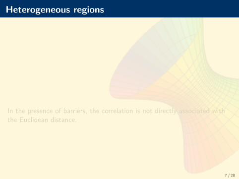
Heterogeneous regions
In the presence of barriers, the correlation is not directly associated withthe Euclidean distance.
7 / 28

Heterogeneous regions
A
A'
B
B'
C
C'
In the presence of barriers, the correlation is not directly associated withthe Euclidean distance.
7 / 28
A practical approach
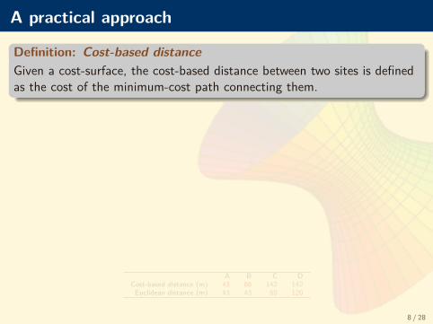
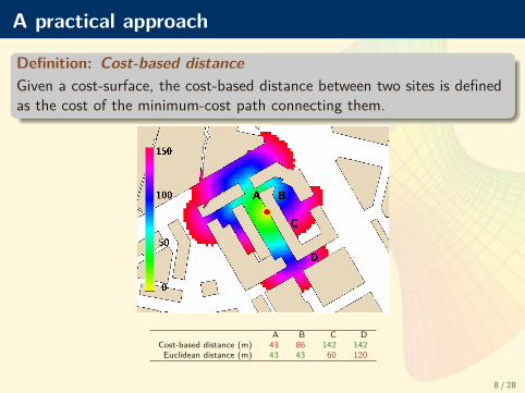
Definition: Cost-based distanceGiven a cost-surface, the cost-based distance between two sites is definedas the cost of the minimum-cost path connecting them.
A B C DCost-based distance (m) 43 86 142 142
Euclidean distance (m) 43 43 60 120
8 / 28
A practical approach
Definition: Cost-based distanceGiven a cost-surface, the cost-based distance between two sites is definedas the cost of the minimum-cost path connecting them.
A B C DCost-based distance (m) 43 86 142 142
Euclidean distance (m) 43 43 60 120
8 / 28

Cost-based geostatistics
I The cost-based distance generalizes the Euclidean distance, which is aparticular case where the cost surface is flat
I It accounts not only for barriers but for general heterogeneous regionsI This definition and its implementation is an original contribution of
the first part of the thesis project
ImplementationI Geographic computation of cost-based distances (GRASS GIS)I Send covariates, observations and prediction locations with
cost-based distance matrices to RI Use (modified) geoR functions to perform cost-based geostatistical
predictionI Return results to GRASS GIS and produce prediction maps
9 / 28
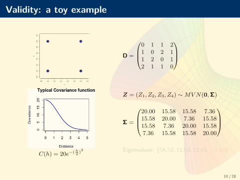
Validity: a toy example
0.8 1.0 1.2 1.4 1.6 1.8 2.0 2.2
0.8
1.0
1.2
1.4
1.6
1.8
2.0
2.2
x
y
1 2
3 4
D =
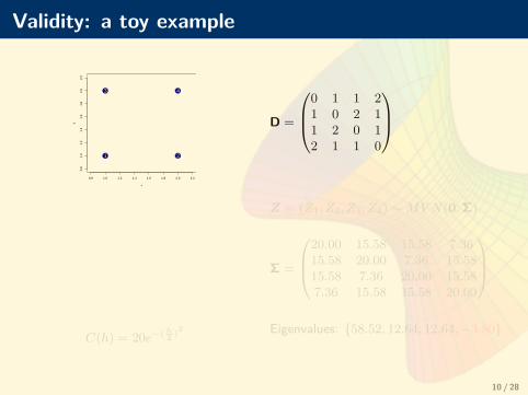
0 1 1 21 0 2 11 2 0 12 1 1 0
C(h) = 20e−( h2 )2
Z = (Z1, Z2, Z3, Z4) ∼MV N(0, Σ)
Σ =
20.00 15.58 15.58 7.3615.58 20.00 7.36 15.5815.58 7.36 20.00 15.587.36 15.58 15.58 20.00
Eigenvalues: 58.52, 12.64, 12.64,−3.80
10 / 28
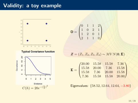
Validity: a toy example
0.8 1.0 1.2 1.4 1.6 1.8 2.0 2.2
0.8
1.0
1.2
1.4
1.6
1.8
2.0
2.2
x
y
1 2
3 4
D =
0 1 1 21 0 2 11 2 0 12 1 1 0
C(h) = 20e−( h2 )2
Z = (Z1, Z2, Z3, Z4) ∼MV N(0, Σ)
Σ =
20.00 15.58 15.58 7.3615.58 20.00 7.36 15.5815.58 7.36 20.00 15.587.36 15.58 15.58 20.00
Eigenvalues: 58.52, 12.64, 12.64,−3.80
10 / 28
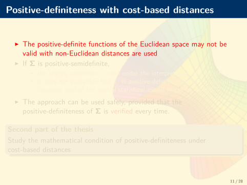
Positive-definiteness with cost-based distances
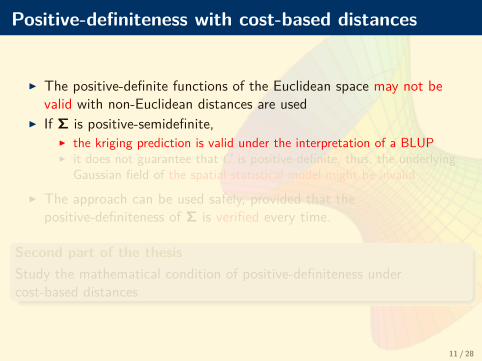
I The positive-definite functions of the Euclidean space may not bevalid with non-Euclidean distances are used
I If Σ is positive-semidefinite,I the kriging prediction is valid under the interpretation of a BLUPI it does not guarantee that C is positive-definite, thus, the underlying
Gaussian field of the spatial statistical model might be invalid
I The approach can be used safely, provided that thepositive-definiteness of Σ is verified every time.
Second part of the thesisStudy the mathematical condition of positive-definiteness undercost-based distances
11 / 28
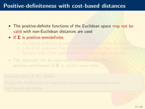
Positive-definiteness with cost-based distances
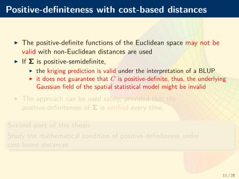
I The positive-definite functions of the Euclidean space may not bevalid with non-Euclidean distances are used
I If Σ is positive-semidefinite,I the kriging prediction is valid under the interpretation of a BLUPI it does not guarantee that C is positive-definite, thus, the underlying
Gaussian field of the spatial statistical model might be invalid
I The approach can be used safely, provided that thepositive-definiteness of Σ is verified every time.
Second part of the thesisStudy the mathematical condition of positive-definiteness undercost-based distances
11 / 28
Positive-definiteness with cost-based distances
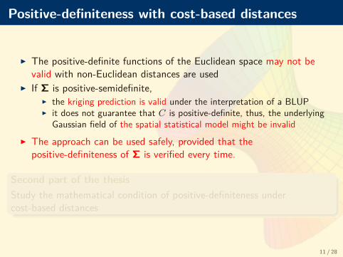
I The positive-definite functions of the Euclidean space may not bevalid with non-Euclidean distances are used
I If Σ is positive-semidefinite,I the kriging prediction is valid under the interpretation of a BLUPI it does not guarantee that C is positive-definite, thus, the underlying
Gaussian field of the spatial statistical model might be invalidI The approach can be used safely, provided that the
positive-definiteness of Σ is verified every time.
Second part of the thesisStudy the mathematical condition of positive-definiteness undercost-based distances
11 / 28
Positive-definiteness with cost-based distances
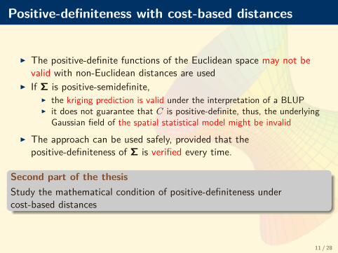
I The positive-definite functions of the Euclidean space may not bevalid with non-Euclidean distances are used
I If Σ is positive-semidefinite,I the kriging prediction is valid under the interpretation of a BLUPI it does not guarantee that C is positive-definite, thus, the underlying
Gaussian field of the spatial statistical model might be invalidI The approach can be used safely, provided that the
positive-definiteness of Σ is verified every time.
Second part of the thesisStudy the mathematical condition of positive-definiteness undercost-based distances
11 / 28
Positive-definiteness with cost-based distances
I The positive-definite functions of the Euclidean space may not bevalid with non-Euclidean distances are used
I If Σ is positive-semidefinite,I the kriging prediction is valid under the interpretation of a BLUPI it does not guarantee that C is positive-definite, thus, the underlying
Gaussian field of the spatial statistical model might be invalidI The approach can be used safely, provided that the
positive-definiteness of Σ is verified every time.
Second part of the thesisStudy the mathematical condition of positive-definiteness undercost-based distances
11 / 28

Riemannian model
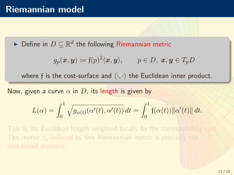
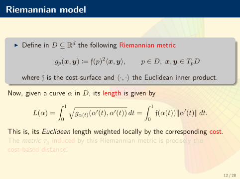
I Define in D ⊆ Rd the following Riemannian metric
gp(x,y) := f(p)2〈x,y〉, p ∈ D, x,y ∈ TpD
where f is the cost-surface and 〈·, ·〉 the Euclidean inner product.
Now, given a curve α in D, its length is given by
L(α) =∫ 1
0
√gα(t)(α′(t), α′(t)) dt =
∫ 1
0f(α(t))‖α′(t)‖ dt.
This is, its Euclidean length weighted locally by the corresponding cost.The metric τg induced by this Riemannian metric is precisely thecost-based distance.
12 / 28
Riemannian model
I Define in D ⊆ Rd the following Riemannian metric
gp(x,y) := f(p)2〈x,y〉, p ∈ D, x,y ∈ TpD
where f is the cost-surface and 〈·, ·〉 the Euclidean inner product.
Now, given a curve α in D, its length is given by
L(α) =∫ 1
0
√gα(t)(α′(t), α′(t)) dt =
∫ 1
0f(α(t))‖α′(t)‖ dt.
This is, its Euclidean length weighted locally by the corresponding cost.The metric τg induced by this Riemannian metric is precisely thecost-based distance.
12 / 28

Positive definiteness in Riemannian manifolds
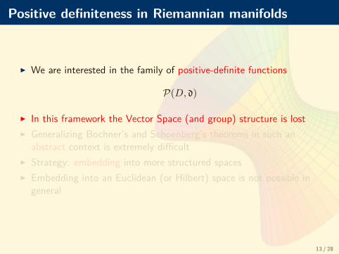
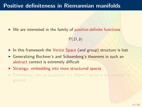
I We are interested in the family of positive-definite functions
P(D, d)
I In this framework the Vector Space (and group) structure is lostI Generalizing Bochner’s and Schoenberg’s theorems in such an
abstract context is extremely difficultI Strategy: embedding into more structured spacesI Embedding into an Euclidean (or Hilbert) space is not possible in
general
13 / 28
Positive definiteness in Riemannian manifolds
I We are interested in the family of positive-definite functions
P(D, d)
I In this framework the Vector Space (and group) structure is lostI Generalizing Bochner’s and Schoenberg’s theorems in such an
abstract context is extremely difficultI Strategy: embedding into more structured spacesI Embedding into an Euclidean (or Hilbert) space is not possible in
general
13 / 28
Positive definiteness in Riemannian manifoldsBanach spaces (algebras)
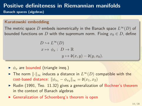
Kuratowski embeddingThe metric space D embeds isometrically in the Banach space L∞(D) ofbounded functions on D with the supremum norm. Fixing x0 ∈ D, define
D → L∞(D)x 7→ φx : D → R
y 7→ d(x, y)− d(y, x0).
I φx are bounded (triangle ineq.)I The norm ‖·‖∞ induces a distance in L∞(D) compatible with the
cost-based distance: ‖φx1 − φx2‖∞ = d(x1, x2)I Rudin (1991, Teo. 11.32) gives a generalization of Bochner’s theorem
in the context of Banach algebrasI Generalization of Schoenberg’s theorem is open
14 / 28
Positive definiteness in Riemannian manifoldsBanach spaces (algebras)
Kuratowski embeddingThe metric space D embeds isometrically in the Banach space L∞(D) ofbounded functions on D with the supremum norm. Fixing x0 ∈ D, define
D → L∞(D)x 7→ φx : D → R
y 7→ d(x, y)− d(y, x0).
I φx are bounded (triangle ineq.)I The norm ‖·‖∞ induces a distance in L∞(D) compatible with the
cost-based distance: ‖φx1 − φx2‖∞ = d(x1, x2)I Rudin (1991, Teo. 11.32) gives a generalization of Bochner’s theorem
in the context of Banach algebrasI Generalization of Schoenberg’s theorem is open
14 / 28

Euclidean representation
An Euclidean representation of a distance matrix D n× n is a matrix Xwhose rows give the coordinates of a set of points x1, . . . ,xn ∈ Rd thatreproduce the distances.
I Not all distance matrices admit an exact Euclidean representation.I The matrix D from the example does not.
15 / 28
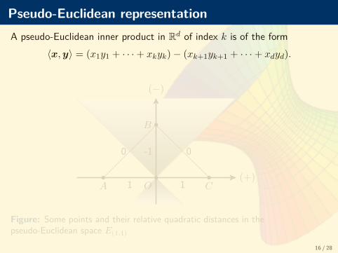
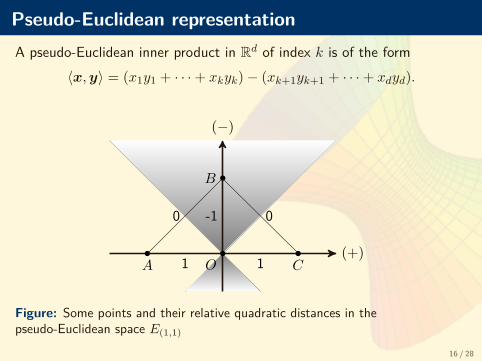
Pseudo-Euclidean representationA pseudo-Euclidean inner product in Rd of index k is of the form
〈x,y〉 = (x1y1 + · · ·+ xkyk)− (xk+1yk+1 + · · ·+ xdyd).
(+)
(−)
OA
B
C
0 0
1 1
-1
Figure: Some points and their relative quadratic distances in thepseudo-Euclidean space E(1,1)
16 / 28
Pseudo-Euclidean representationA pseudo-Euclidean inner product in Rd of index k is of the form
〈x,y〉 = (x1y1 + · · ·+ xkyk)− (xk+1yk+1 + · · ·+ xdyd).
(+)
(−)
OA
B
C
0 0
1 1
-1
Figure: Some points and their relative quadratic distances in thepseudo-Euclidean space E(1,1)
16 / 28
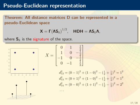
Pseudo-Euclidean representation
Theorem: All distance matrices D can be represented in apseudo-Euclidean space
X = Γ(ΛSk
)1/2, HDH = ΛSkΛ,
where Sk is the signature of the space.
0.8 1.0 1.2 1.4 1.6 1.8 2.0 2.2
0.8
1.0
1.2
1.4
1.6
1.8
2.0
2.2
x
y
1 2
3 4
X =
0 1 1
21 0 −1
2−1 0 −1
20 −1 1
2
d2
12 = (0− 1)2 + (1− 0)2 − ( 12 + 1
2 )2 = 12
d213 = (0 + 1)2 + (1− 0)2 − ( 1
2 + 12 )2 = 12
d214 = (0− 0)2 + (1 + 1)2 − ( 1
2 −12 )2 = 22
. . .
17 / 28
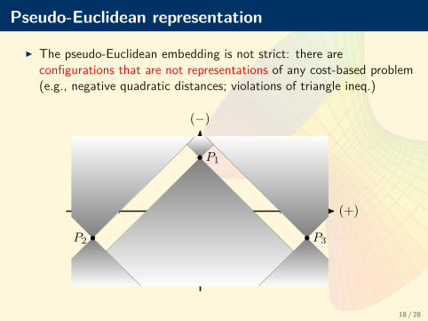
Pseudo-Euclidean representation
I The pseudo-Euclidean embedding is not strict: there areconfigurations that are not representations of any cost-based problem(e.g., negative quadratic distances; violations of triangle ineq.)
(+)
(−)
P1
P2 P3
18 / 28
Positive definiteness in pseudo-Euclidean spaces
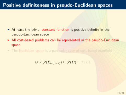
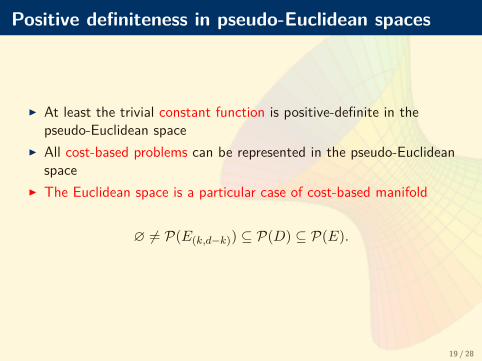
I At least the trivial constant function is positive-definite in thepseudo-Euclidean space
I All cost-based problems can be represented in the pseudo-Euclideanspace
I The Euclidean space is a particular case of cost-based manifold
∅ 6= P(E(k,d−k)) ⊆ P(D) ⊆ P(E).
19 / 28
Positive definiteness in pseudo-Euclidean spaces
I At least the trivial constant function is positive-definite in thepseudo-Euclidean space
I All cost-based problems can be represented in the pseudo-Euclideanspace
I The Euclidean space is a particular case of cost-based manifold
∅ 6= P(E(k,d−k)) ⊆ P(D) ⊆ P(E).
19 / 28
Generalizations of Bochner’s and Schoenberg’stheorems
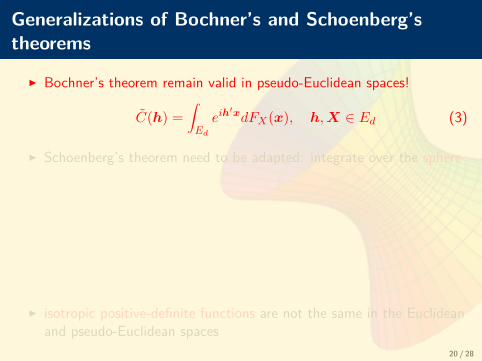
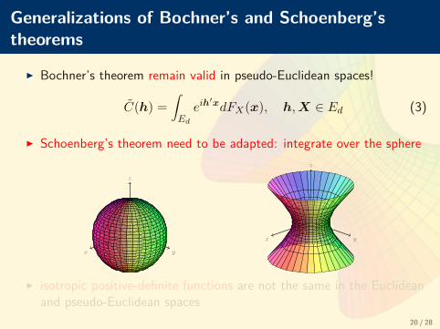
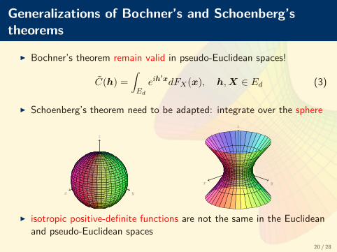
I Bochner’s theorem remain valid in pseudo-Euclidean spaces!
C(h) =∫Ed
eih′xdFX(x), h,X ∈ Ed (3)
I Schoenberg’s theorem need to be adapted: integrate over the sphere
x y
z
x y
z
I isotropic positive-definite functions are not the same in the Euclideanand pseudo-Euclidean spaces
20 / 28
Generalizations of Bochner’s and Schoenberg’stheorems
I Bochner’s theorem remain valid in pseudo-Euclidean spaces!
C(h) =∫Ed
eih′xdFX(x), h,X ∈ Ed (3)
I Schoenberg’s theorem need to be adapted: integrate over the sphere
x y
z
x y
z
I isotropic positive-definite functions are not the same in the Euclideanand pseudo-Euclidean spaces
20 / 28

Integrating on the hyperboloid
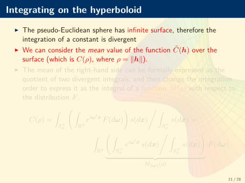
I The pseudo-Euclidean sphere has infinite surface, therefore theintegration of a constant is divergent
I We can consider the mean value of the function C(h) over thesurface (which is C(ρ), where ρ = ‖h‖).
I The mean of the right-hand side can be formally expressed as thequotient of two divergent integrals, and then change the integrationorder to express it as the integral of a function M(ρ) with respect tothe distribution F .
C(ρ) =∫S+ρ
(∫Rdeiω′x F (dω)
)s(dx)
/∫S+ρ
s(dx) =
∫Rd
(∫S+ρ
eiω′x s(dx)
/∫S+ρ
s(dx))
︸ ︷︷ ︸M‖ω‖(ρ)
F (dω).
21 / 28
Integrating on the hyperboloid
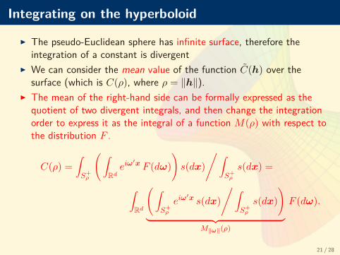
I The pseudo-Euclidean sphere has infinite surface, therefore theintegration of a constant is divergent
I We can consider the mean value of the function C(h) over thesurface (which is C(ρ), where ρ = ‖h‖).
I The mean of the right-hand side can be formally expressed as thequotient of two divergent integrals, and then change the integrationorder to express it as the integral of a function M(ρ) with respect tothe distribution F .
C(ρ) =∫S+ρ
(∫Rdeiω′x F (dω)
)s(dx)
/∫S+ρ
s(dx) =
∫Rd
(∫S+ρ
eiω′x s(dx)
/∫S+ρ
s(dx))
︸ ︷︷ ︸M‖ω‖(ρ)
F (dω).
21 / 28
Integrating on the hyperboloid
I The pseudo-Euclidean sphere has infinite surface, therefore theintegration of a constant is divergent
I We can consider the mean value of the function C(h) over thesurface (which is C(ρ), where ρ = ‖h‖).
I The mean of the right-hand side can be formally expressed as thequotient of two divergent integrals, and then change the integrationorder to express it as the integral of a function M(ρ) with respect tothe distribution F .
C(ρ) =∫S+ρ
(∫Rdeiω′x F (dω)
)s(dx)
/∫S+ρ
s(dx) =
∫Rd
(∫S+ρ
eiω′x s(dx)
/∫S+ρ
s(dx))
︸ ︷︷ ︸M‖ω‖(ρ)
F (dω).
21 / 28
Divergence of the function M
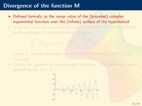
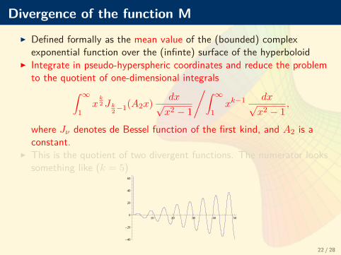
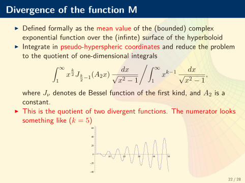
I Defined formally as the mean value of the (bounded) complexexponential function over the (infinte) surface of the hyperboloid
I Integrate in pseudo-hyperspheric coordinates and reduce the problemto the quotient of one-dimensional integrals∫ ∞
1xk2 J k
2−1(A2x) dx√x2 − 1
/∫ ∞1
xk−1 dx√x2 − 1
,
where Jν denotes de Bessel function of the first kind, and A2 is aconstant.
I This is the quotient of two divergent functions. The numerator lookssomething like (k = 5)
10 20 30 40 50
-40
-20
0
20
40
60
22 / 28
Divergence of the function M
I Defined formally as the mean value of the (bounded) complexexponential function over the (infinte) surface of the hyperboloid
I Integrate in pseudo-hyperspheric coordinates and reduce the problemto the quotient of one-dimensional integrals∫ ∞
1xk2 J k
2−1(A2x) dx√x2 − 1
/∫ ∞1
xk−1 dx√x2 − 1
,
where Jν denotes de Bessel function of the first kind, and A2 is aconstant.
I This is the quotient of two divergent functions. The numerator lookssomething like (k = 5)
10 20 30 40 50
-40
-20
0
20
40
60
22 / 28
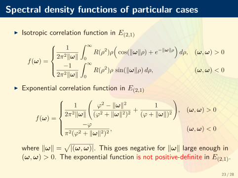
Spectral density functions of particular cases
I Isotropic correlation function in E(2,1)
f(ω) =
1
2π2‖ω‖
∫ ∞0
R(ρ2)ρ(
cos(‖ω‖ρ) + e−‖ω‖ρ)dρ, (ω,ω) > 0
−12π2‖ω‖
∫ ∞0
R(ρ2)ρ sin(‖ω‖ρ) dρ, (ω,ω) < 0
I Exponential correlation function in E(2,1)
f(ω) =
1
2π2‖ω‖
(ϕ2 − ‖ω‖2
(ϕ2 + ‖ω‖2)2 + 1(ϕ+ ‖ω‖)2
), (ω,ω) > 0
−ϕπ2(ϕ2 + ‖ω‖2)2 , (ω,ω) < 0
where ‖ω‖ =√|(ω,ω)|. This goes negative for ‖ω‖ large enough in
(ω,ω) > 0. The exponential function is not positive-definite in E(2,1).
23 / 28
Reparameterization of covariance matrices
I Model the elements of a reparameterization of the covariance matrix(e.g. Cholesky) as a function of the distances
I We still want covariances to be functions of the distancesI We need all possible covariance matrices to be positive-definiteI No significant progress on this line
24 / 28
Markov approximations of Matérn fields
I S different approach to irregular regionsI The resulting correlations structure is different from cost-basedI The approach works well, although is less general and has some other
issues (e.g., border effects)
25 / 28
Markov approximations of Matérn fields
I S different approach to irregular regionsI The resulting correlations structure is different from cost-basedI The approach works well, although is less general and has some other
issues (e.g., border effects)
25 / 28
Markov approximations of Matérn fields
I S different approach to irregular regionsI The resulting correlations structure is different from cost-basedI The approach works well, although is less general and has some other
issues (e.g., border effects)
25 / 28
Conclusions
I Thesis topic: Geostatistical prediction in heterogeneous regionsI Main contribution 1: The cost-based methodology. A practical and
applied approach, and its implementation.I Main contribution 2: The mathematical framework of the problem of
positive-definiteness with cost-based distances.I Main contribution 3: Investigation of possible approaches.
Pseudo-Euclidean embedding theorem. Formulas for the spectraldensity of an isotropic function in E(2,1).
26 / 28

Open lines of work
I Combine the cost-based approach with the outcome of a ComputerModel of noise diffusion
I Elaborate known results about positive-definite functions on BanachAlgebras (Rudin, 1991; Berg et al., 1984)
I Elaborate the isotropy characterization of stationary functions underthe action of a group over the manifold, considering a generalizedFourier transform with respect to the Hausdorff measure
I Mean value of a function over the d-dimensional hyperboloidI Search positive-definite functions on the pseudo-Euclidean space
using the formulas for the spectral density of isotropic functionsI Brute-force investigation of positive-definiteness for candidate
functions
27 / 28

Facultat de Ciències MatemàtiquesDepartament d’Estadística i Investigació Operativa
Geoestadística en regiones heterogéneas condistancia basada en el coste
TESIS DOCTORALFacundo Martín Muñoz Viera
Director: Antonio López-QuílezFebrero 2013